Technology differences, institutions and economic growth ... · TECHNOLOGY DIFFERENCES,...
65
No 2004 – 02 Technology differences, institutions and economic growth : a conditional conditional convergence _____________ Hervé Boulhol
Transcript of Technology differences, institutions and economic growth ... · TECHNOLOGY DIFFERENCES,...
No 2004 – 02
Technology differences, institutions and economicgrowth : a conditional conditional convergence
_____________
Hervé Boulhol

Technology differences, institutions and economicgrowth : a conditional conditional convergence
_____________
Hervé Boulhol
No 2004 – 02 February

Technology differences, institutions and economic growth :a conditional conditional convergence
3
TABLE OF CONTENTS
SUMMARY..............................................................................................................................................4
ABSTRACT..............................................................................................................................................5
RÉSUMÉ..................................................................................................................................................6
RÉSUMÉ COURT....................................................................................................................................7
1. INTRODUCTION ...........................................................................................................................8
2. TECHNOLOGY DIFFERENCES AND DIFFUSION.....................................................................10
3. GROWTH EQUATIONS AND INSTITUTIONS ...........................................................................11
4. DATA ............................................................................................................................................13
5. FROM THE INSTITUTIONAL DATABASE TO THE ECONOMETRIC SPECIFICATION........15
6. RESULTS ......................................................................................................................................17
7. CONCLUSION..............................................................................................................................24
BIBLIOGRAPHY...................................................................................................................................25
APPENDIX 1..........................................................................................................................................38
APPENDIX 2..........................................................................................................................................41
APPENDIX 3..........................................................................................................................................45
APPENDIX 4..........................................................................................................................................46
LIST OF WORKING PAPERS RELEASED BY CEPII ..........................................................................58

CEPII, Working Paper No 2004 - 02
4
TECHNOLOGY DIFFERENCES , INSTITUTIONS AND ECONOMIC GROWTH : ACONDITIONAL CONDITIONAL CONVERGENCE
SUMMARY
The augmented Solow model by Mankiw, Romer and Weil (1992) exhibited the role ofhuman capital for long term growth path and led its authors to accept either the assumptionof identical technology across countries or the treatment of technology differences asresiduals in the growth equation. However, Hall and Jones (1996, 1999) and Klenow andRodriguez-Clare (1997) have shown that productivity levels and output per worker arehighly correlated, which casts doubts on the conditional convergence scenario. Yet thecross section literature has not drawn the necessary implications. Acknowledging theimportance of taking into account productivity differences, we break down productivityinto two components: a pure technological part and its complement called “efficiency”.From a simple model of technology diffusion, we focus on the interactions betweeninstitutions and technology differences and identify three complementary channels throughwhich institutions impact growth: efficiency in the use of technology, long term TFP-growth and technology diffusion.
To shed light on how growth and institutions interplay, our framework is tested from a newand detailed database on institutions developed by the French Ministry of Economy,Finance and Industry (MINEFI). Data was collected through a questionnaire by theEconomic Missions of the MINEFI in 51 countries representing 80% of world GDP. Thedatabase consists of 330 items on institutions in a broad sense, each receiving a rankingfrom 0 to 4 for each country. The robustness of the database has been established byBerthelier, Desdoigts and Ould-Aoudia (2003) through a comparative study with otherinstitutional databases used in various economic studies.
We find that technology diffusion substantially impacts economic performance and thatcatching-up is conditional to the quality of the appropriate institution – a mix of R&D,innovation and capital-risk support -, with the annual rate of convergence to thetechnological frontier varying from 0% to 12.4% depending on the country. Institutionsalso matter for technological efficiency, as our non-corruption variable, for instance,contributes as much as the stock of human capital to the productivity level heterogeneity.Moreover, long run TFP-growth differences are significantly determined by suchinstitutions like the ones reflecting a competitive product market or a favourable innovationenvironment. Having controlled for institutions, international trade measured, by theopenness rate, is insignificant to explain neither TFP-growth differences nor technologydiffusion. However, when we take the manufacturing share in exports into account, we finda significant impact of trade on TFP-growth, coming solely from the richer countries in thesample, which clearly points to a non-linearity. This suggests that the contribution of tradeis positive only if the specialisation is appropriate and the development fairly advanced.This last result is tentative because of potential endogeneity biases. Including human capitalflows as a determinant of the steady-state reveals that MRW’s approach and ours are

Technology differences, institutions and economic growth :a conditional conditional convergence
5
complements rather than substitutes. Conditional convergence here is also conditional tosharing the same technology and quality of institutions, which renders recent observeddivergence well accounted for.
ABSTRACT
Highlighting that technology is only a component of productivity, this study focuses on theinteractions between institutions and technology differences to explain cross-countrygrowth pattern. Three complementary channels through which institutions impact growthare identified: efficiency in the use of technology, long term TFP-growth and technologydiffusion. From a new and detailed database on institutions developed by the FrenchMinistry of Economy, Finance and Industry, poor institutional quality, beyond humancapital, is estimated to be the source of an annual growth-rate loss of between 2.4 and 6.1percentage point for half of the countries. Technology diffusion speed is institutionallyrelated and the distance to the technology frontier is reduced from 0% to 12.4% annuallydepending on the country. Trade has a non linear influence on growth, being significantonly for countries already advanced in the development phase. Conditional convergencehere is also conditional to sharing the same technology and quality of institutions, renderingrecent observed divergence well accounted for.
J.E.L. classification: O11; O33; O47Keywords: Technology diffusion; Institutions; Productivity; Growth

CEPII, Working Paper No 2004 - 02
6
ECARTS TECHNOLOGIQUES , INSTITUTIONS ET CROISSANCE ÉCONOMIQUE: UNECONVERGENCE CONDITIONNELLE CONDITIONNELLE
RÉSUMÉ
L’extension du modèle de Solow par Mankiw, Romer et Weil (1992) a mis en évidence lerôle du capital humain pour le sentier de croissance à long terme et a conduit ses auteurs àaccepter l’hypothèse d’une technologie identique pour l’ensemble des pays ou le traitementdes différences technologiques comme résidus des équations de croissance. Hall et Jones(1996, 1999) et Klenow et Rodriguez-Clare (1997) ont cependant montré que les niveauxde productivité et de production par tête étaient fortement corrélés, remettant en cause lescenario de convergence conditionnelle, sans que la littérature en ait tiré toutes lesimplications qui s’imposent. Reconnaissant l’enjeu de la prise en compte des différences deproductivité, nous décomposons la productivité en deux éléments : une composantepurement technologique et son complément que nous appelons « efficacité ». A partir d’unmodèle simple de diffusion technologique, nous nous concentrons sur les interactions entreles institutions et les différences de technologies pour expliquer l’évolution comparée de lacroissance entre pays. Trois canaux complémentaires par lesquels les institutions ont uneinfluence sur la croissance sont identifiés: l’efficacité dans l’utilisation des technologies, lacroissance de la productivité à long terme et la diffusion des technologies.
Pour clarifier les interactions entre les institutions et la croissance économique, notremodèle est testé à partir d’une nouvelle base de données institutionnelles détaillée,développée par le MINEFI. Les données ont été collectées par les Missions Economiquesdu MINEFI dans 51 pays représentant 80% du PIB mondial. La base de donnée estcomposée de 330 items sur les institutions, notion prise dans son sens large, chacun d’entreeux recevant une note entre 0 et 4 pour chaque pays. Berthelier, Desdoigts et Ould-Aoudia(2003) ont établi la robustesse de la base en la rapprochant d’autres bases de donnéesinstitutionnelles utilisées dans les travaux économiques.
Nous trouvons que la diffusion technologique a un impact substantiel sur la performanceéconomique et que le rattrapage est conditionnelle à la qualité de l’institution adéquate – unmélange de R&D, d’innovation et de support au capital-risque -, avec une vitesse annuellede convergence vers la frontière technologique variant de 0% à 12,4% selon les pays. Lesinstitutions importent aussi pour l’efficacité dans l’utilisation des technologies, et notremesure de la non-corruption, par exemple, contribue autant que le stock de capital humain àla dispersion de la productivité. De plus, les différences de croissance de la productivitétotale des facteurs (PTF) à long terme sont significativement déterminées par desinstitutions telles que celles reflétant un marché des produits concurrentiel ou unenvironnement favorable à l’innovation. En contrôlant les différences institutionnelles, lecommerce international, mesuré par le taux d’ouverture, n’est significatif ni pour expliquerles différences de croissance de la PTF ni pour la diffusion des technologies. Cependant,lorsque l’on prend en compte la part des biens manufacturés dans les exportations, alorsnous trouvons un impact significatif du commerce sur la croissance de la PTF, provenant

Technology differences, institutions and economic growth :a conditional conditional convergence
7
seulement des pays les plus riches dans l’échantillon, ce qui indique une non-linéarité. Celasuggère que la contribution du commerce est positive seulement si la spécialisation estappropriée et le développement déjà avancé. Ce dernier résultat est fragile en raisond’éventuels biais d’endogénéité. De plus, la prise en compte de l’impact du flux de capitalhumain pour l’état régulier révèle que l’approche de MRW et la notre sont descompléments plutôt que des substituts. La convergence conditionnelle est ici conditionnelleaussi au fait de disposer des mêmes technologies et des mêmes institutions, et rend comptede la divergence récemment observée.
RÉSUMÉ COURT
Insistant sur la distinction entre productivité et technologie, cette étude se concentre sur lesinteractions entre les institutions et les écarts de technologiques pour expliquer l’évolutioncomparée de la croissance entre pays. Trois canaux complémentaires par lesquels lesinstitutions ont une influence sur la croissance sont identifiés: l’efficacité dans l’utilisationdes technologies, la croissance de la productivité à long terme et la diffusion destechnologies. A partir d’une nouvelle base de données institutionnelles détaillée,développée par le MINEFI, nous estimons que l’insuffisante qualité des institutions, au-delàdu capital humain, est la cause d’un déficit de taux de croissance annuelle entre 2,4 et 6,1point de pourcentage pour la moitié des pays. La vitesse annuelle de diffusion destechnologies varie de 0% à 12,4% selon les pays en fonction de leur niveau institutionnel.Le commerce a un impact non linéaire sur la croissance puisqu’il est significatif seulementpour les pays déjà avancés dans la phase de développement. La convergence conditionnelleest ici conditionnelle aussi au fait de disposer des mêmes technologies et de la mêmequalité des institutions, et rend compte de la divergence récemment observée.
J.E.L. classification: O11 ; O33 ; O47Mots-clés: Diffusion des technologies ; Institutions ; Productivité ; Croissance

CEPII, Working Paper No 2004 - 02
8
TECHNOLOGY DIFFERENCES , INSTITUTIONS AND ECONOMIC GROWTH : ACONDITIONAL CONDITIONAL CONVERGENCE (*)
Hervé Boulhol
1. INTRODUCTION
The seminal article by Mankiw, Romer and Weil (1992), subsequently denoted MRW, shedlight on the contribution of human capital in reconciling the measured low speed ofconditional convergence between countries with a physical capital share of around one-third. Their main conclusion is that, when human capital is added, the then augmentedSolow model is well suited to analyse growth across countries. It follows that, contrary toendogenous growth theory, the growth process is solely driven by factor accumulation(including human capital), is consistent with a rate of convergence of around 2% a year(rather than the 4%-5% expected from the Solow textbook model) and validates underlyingassumptions of constant returns to scale and identical technology. The MRW frameworkhas been criticised on different grounds. First, the embedded human capital theory treatshuman capital just as another accumulating factor. This implies that human capital shouldenter into growth equation through its growth rate, but there is confusion in whether thestock of human capital matters rather than the flow as in MRW. Benhabib and Spiegel(1994) convincingly support the view that the stock of human capital is a “determinant ofthe magnitude of a country’s Solow residual”. Second, as most of the cross-countryliterature, the MRW approach is subject to the bias coming from the identical technologyassumption.
The conditional convergence predictions has been more and more difficult to reconcile withthe facts pointing to global divergence as outlined by Pritchett (1997). Prompted byJ.Temple’s fourth question about the causes of income differences (Temple, 1999, p.113),we start from the inference that if poor countries are poor not only because of a lack ofinputs that will accumulate faster fostering convergence, it must be that they are poor alsobecause of overall efficiency and technology differentials - whatever these mean - that maypersist or aggravate over time especially if they are due to institutional differences.
1 The
role of institutions as a determinant of long term growth is increasingly recognised, yetmore research is needed to disentangle which institutions matter for economic performanceand above all to incorporate them properly in economic theory. Even though Rodrik (2002,2003) is convincing in arguing that the same institutions may have different economic
(*): I would like to express my gratitude to Lionel Fontagné, Jacques Ould-Aoudia and Patrick Artus forhaving made this study possible. I would particularly like to thank Agnès Bénassy-Quéré, GuillaumeGaulier, Romain Rancière and the participants of the Cepii seminar for their valuable comments. Finally Ivery much appreciated the help I received from Maylis Coupet and David Galvin, as well as the warmwelcome I received from Cepii employees.1 ‘’ (Q4) Are poor countries poor mainly because they lack inputs, or because of technology differences? ‘’

Technology differences, institutions and economic growth :a conditional conditional convergence
9
impacts based on a country’s idiosyncrasies, we suggest that the quality of some institutionsdoes influence economic performance overall. In this study, we show that technologydifferences play an important role in the cross-country growth pattern and that institutionsmatter for total factor productivity (TFP) level and growth rates, and for technologydiffusion.
Many reasons may explain why technology differs significantly between countries. Patentprotection, learning by doing, knowledge differences detract technology from its public-good pretension (Caselli, Esquivel and Lefort, 1996). Moreover, taking a broader view ofproductivity, institutions linked to the social, political or legal aspects of efficiencycontribute to productivity differentials. Surprisingly, the growth literature does not payenough attention to heterogeneity in technology. When it does, this heterogeneity is treatedin panel estimates and as a fixed effect, the details of which are rarely available, making anassessment of whether they do represent what they should difficult. Exceptions are Hall andJones (1996, 1999), Klenow and Rodriguez-Clare (1997) who precisely estimateproductivity differences and Bloom, Canning and Sevilla (2002) whose concerns are closeto ours. We hope our contribution to be theoretical and empirical. Theoretically we identifythree channels through which institutions may impact productivity. First, a staticcontribution through efficiency in the use of technology, second a persistent dynamic onethrough long run TFP-growth rates and third a temporary dynamic one through technologydiffusion. Empirically we test our framework using a new and detailed database oninstitutions that was developed by the French Ministry of Economy, Finance and Industry(MINEFI). Data from a questionnaire was collected by the Economic Missions of theMINEFI in 51 countries representing 80% of world GDP. The database consists of 330items on institutions in a broad sense, each receiving a ranking from 0 to 4 for each country.
We find that technology diffusion substantially impacts economic performance and thatcatching-up is conditional to the quality of the appropriate institution – a mix of R&D,innovation and capital-risk support -, with the annual rate of convergence to thetechnological frontier varying from 0% to 12.4% depending on the country. Institutionsalso matter for technological efficiency, as our non-corruption variable, for instance,contributes as much as the stock of human capital to the productivity level heterogeneity.Moreover, long run TFP-growth differences are significantly determined by suchinstitutions like the ones reflecting a competitive product market or a favourable innovationenvironment. In addition, including human capital flows as a determinant of the steady-state reveals that MRW’s approach and ours are complements rather than substitutes.Having controlled for institutions, international trade measured, by the openness rate, has anon-linear contribution to TFP-growth, being significant and positive only if thespecialisation is appropriate and the development fairly advanced. This last result istentative because of potential endogeneity biases.
The study is organised as follows. Section 2 highlights the importance of taking intoaccount technology differences and introduces our approach regarding the technologicalprocess. Section 3 details how institutions and growth interplay in the model. Section 4describes the data and the selection of the institutional variables, leading to the econometric

CEPII, Working Paper No 2004 - 02
10
specification in Section 5. Results are presented in Section 6 where econometric issues arealso discussed. Finally, Section 7 concludes.
2. TECHNOLOGY DIFFERENCES AND DIFFUSION
The most disputable critical assumption in the cross-section growth literature suggests thateither all countries share the same level of technology and technological progress or that thedifferences in these levels are treated as residuals, implying that they are being consideredindependent from other explanatory variables. This is an extreme conjecture since it meansthat technological change spreads instantaneously and completely to every country,whatever the level of openness or institutional profile, and leads to having only thedifferences of capital per unit of labour to explain differences of output per capita.Assuming a Cobb-Douglas production function and with standard notations,
baii
bi
aii LAHKY −−= 1)(. (1)
where Y is output, K and H are stocks of physical and human capital respectively, A is theproductivity level and L the number of workers. Output per worker iy for the country i is
therefore given by
ai
KHi
bai
bii
aii
baiiii LZALHLKALYy )/.()/.()/.(/ 11 −−−− ≡=≡ (2)
with abKH LHKZ /)/.(= defining a capital aggregate built from the physical capital stock
and the human capital stock per capita. If we assume that the productivity level iA is
independent of the country ( iAAi ∀= , ), then the ratio of output per capita in 1980
between the USA and Uganda of 48 to 1, being the two extremes in our data, translates intoa highly unrealistic capital aggregate, KHZ , per capita ratio of 110,700 to 1 using aphysical capital share of one-third. Moreover, recognising the productivity differences, it isapparent from equation (2), valid at each time, that both the initial productivity level andthe initial output per capita are closely linked, which renders growth equation estimatesassuming identical productivity seriously biased. While this inconvenience is well-acknowledged, the growth literature has not drawn yet all the necessary implications.
Over the last fifteen tears, economic research has made some notable advances in theunderstanding of what productivity is. However, the essence of its contents remainsunknown, and the parameter A is often indistinctly designated as either the productivity orthe technology level. This creates confusion in identifying the role of technology andtherefore, adopting a different posture, we insist here on the distinction between the twonotions and call the complement of technology in productivity: “efficiency”. Inspired byBassanini and Scarpetta (2001), we break down the total level of productivity iA into two
components: a pure technology level iB and the degree of efficiency in using this
technology iX so that iA equals ii XB . . As the benchmark, the country with the highest
GDP per capita in 1980, the USA, has been chosen. We denote benii BBb /= , an inverse

Technology differences, institutions and economic growth :a conditional conditional convergence
11
indicator of the distance to the frontier, benii XXx /= , the ratio of the relative efficiency
to the benchmark, and iibenii xbAAa ./ == , the relative productivity level. Institutional
quality is considered as impacting the technological efficiency iX and possibly the
technology diffusion which process is most simply governed by:2
))(1.()( tbvtb iii −=& (3)
where t stands for time: in the long run technologies converge to the frontier at a pacerepresented by iv , which will be tested as being constant across countries or institutionally-
related. Note it is only the pure technology component that is assumed to converge (ordiverge if iv is negative), and total productivity discrepancies may persist as a result of
differences in institutionally-related efficiency iX .
3. GROWTH EQUATION AND INSTITUTIONS
We suppose that institutions enter into growth equations through three different channels:the level of technological efficiency, the progress of technological efficiency and possiblythe speed of technology diffusion. Noticing that the productivity level iA can be written as
iiben bxA .. , we can split TFP-growth into three components:
i
i
i
i
ben
ben
i
i
bb
xx
AA
AA &&&&
++= (4)
The first term on the right is simply the benchmark TFP-growth, denoted by g, the second,denoted ic− , is the long run TFP-growth deficit to the benchmark and the third is the
technological catch-up component derived from resolving the differential equation (3).
))0(1(
))0(1.(.
itv
iii
i
i
be
bvcg
AA
i −−
−+−=
&(5)
Institutions will have an impact through )0(iX , through ic , and potentially through iv .
We now need to integrate equation (5) into the growth equation. The growth model we thendevelop is the augmented Solow model enriched to take into account the heterogeneity oftechnologies and the contribution of institutions. With in denoting the population growth, d
the physical and human capital depreciation rate, Kis and H
is the fraction of total income
invested in physical and human capital respectively, Appendix 1 establishes the followinggrowth equation:
2 In a recent paper, Benhabib and Spiegel (2003) refers to this diffusion process, originating in the Nelson-
Phelps model, as the confined exponential diffusion process.

CEPII, Working Paper No 2004 - 02
12
))0((
)(
).()(.
1)0().0(
)0(.
1)0()(
,
)1/(1..
itvi
ba
baii
bHi
aKi
t
beni
it
ii
bfcg
cgdn
ssLog
te
Aay
Logt
et
yLogtyLog ii
+−+
−++
−+
−−=
−−−
+
−− ββ
(6)
where )).(1( iii cgdnba −++−−=β is the usual speed of conditional convergence and
the last term
−≈
−−=
−
iii
tvi
itv vbb
ebLog
tbf
i
.1)0(
1)0()).0(1(1
.1
))0((.
, (7)
is the contribution of technology diffusion to growth: it is positively related to the speed ivand to the distance to the technological frontier. Equation (6) is to be compared to theaugmented-Solow growth equation which is exactly the same as if we assume that initialtotal productivity level )0(iA is identical across countries, that every country is at the
frontier )1( =ib and that there is no long term TFP-growth differences )0( =ic . The
growth process is therefore the result of four distinct forces: the “adjusted” absoluteconvergence – this source of convergence is lessened here because of overall productivitylevel differences, therefrom the adjective “adjusted” -, a second convergence componentcoming from technological catch-up, the usual non-convergence stemming from differencesin long term paths due to different investment rates and an additional divergence forcecoming from long term TFP-growth differences.
The main reason for considering that all countries share the same technology lies in thedifficulty to observe relative technology levels. What is only needed here, as shown byequation (6), is the relative level of initial productivity and there is one piece of informationfrom which we can estimate it. Indeed equation (2) illustrates that initial output per workeris certainly linked to initial productivity. We will assume that a part η of initial incomeratios can be explained by initial productivity ratios, the complement η−1 being explained
by capital differences, and therefore we formally write:
η
=≡
)0()0(
)0(
)0()0(
ben
i
ben
ii y
y
A
Aa (8a)
Hence η is characterised by:
))0(())0(),0((
i
ii
yLogVaryLogaLogCov
=η (8b)
Klenow and Rodriguez-Clare (1997) use estimates of stocks of physical and human capitalto infer productivity levels and assess that “productivity differences account for half ormore of level differences in 1985 GDP per worker” (p.75). For instance according to

Technology differences, institutions and economic growth :a conditional conditional convergence
13
equation (2), with 75.0=η and 3/1== ba , the output per capita ratio between the USA
and Uganda of 48 in 1980 is “explained” by a contribution from the productivity level ratioof 2.7 and a capital aggregate, KHZ , per capita ratio of 6,100 instead of 110,700. For sure,the extreme simplification in equation (8a), which has though the merit of highlighting thepotential correlation between initial productivity and initial output per worker, and ofavoiding the main pitfall of the cross-section approach, is a strong ad hoc assumption, buttaking 0=η , as is done in most of the cross-section literature, is as strong and certainly a
far more inaccurate ad hoc assumption.
4. DATA
4.1. General data
The time frame is the period from 1980 to 2000. For data entering the traditional Solowmodel, we use Penn World Table 6.1.
3 The per capita output is the real GDP per capita at
Purchasing Power Parity, chain series. For the investment rate Kis , we use the average over
the period of the investment share of real GDP (variable ki in the database). As in MRW,the proxy for the rate of human capital accumulation is the percentage of the working-agepopulation in second-level education. This percentage is constructed by multiplying thegross secondary enrollment rate (World Development Indicators) by the percentage of theworking-aged population aged 15 to 19. The average of this variable over the years 1980,1990 and 2000 is named HCFLOW.
4.2. Institutions database
We use an original database on institutions developed by the MINEFI, well described andanalysed in Berthelier, Desdoigts and Ould-Aoudia (2003). This database focuses primarilyon emerging countries as 44 of the 51 countries are developing countries and also includesa control group of developed countries. Data was gathered from a very detailedquestionnaire: for each country, 330 items aggregated in 115 indicators were madeavailable. As an example the indicator related to the efficiency of public policy linked tothe quality of the tax system is built from four items assessing the importance of the blackmarket, the importance of fraud in the formal economy, in customs and the capacity of theAdministration to implement tax measures. Importantly, Berthelier et al have establishedthe robustness of the database by highlighting its convergence with various institutionaldatabases (World Bank, Fraser Institute, Economist Intelligence Unit, Political EconomicRisk Consultancy, IMF, Transparency International among others) all covering 30% of thestock variables from the questionnaire. The limitations of the database are twofold: a fairlysmall number of countries and a time period limited to a single point in or close to year2000. We will consider that the institutional profile for a given country is stable over the
3 Alan Heston, Robert Summers and Bettina Aten, Penn World Table Version 6.1, Center for International
Comparisons at the University of Pennsylvania (CICUP), October 2002.

CEPII, Working Paper No 2004 - 02
14
period of the growth analysis. This raises poisonous questions of endogeneity since acountry experiencing a favourable economic development increases its chances ofdeveloping better institutions and the causality between growth and institutions might bereversed. Therefore, those indicators that are too suspicious in this respect are excluded andthis endogeneity issue is econometrically addressed in section 6.4.
For the purpose of the study, we cluster the remaining 94 indicators into five groupsrepresenting distinct aspects of the institutional profile. These five institutional domainscover product market, labour market, financial system, innovation and a general heading forall other indicators. Each domain is analysed through a factor analysis which aggregates theoriginal indicators and provides robust institutional variables synthesising most of theinformation in the database.
4.3. Factor Analysis
The chosen approach is very close to that of Nicoletti, Scarpetta and Boylaud (1999)developed to build product market regulation indicators. It differs only in the factorsaggregation methodology and details are found in Appendix 2. The idea is simple: for eachdomain, we run a factor analysis and select the number of relevant factors according tousual tests. The axes are then rotated in order to enhance interpretation of factors and anaggregated index is built for each domain. Unsurprisingly these aggregated indices areextremely correlated with each other so that valuable detailed information is lost in theaggregation process. As a consequence we preferred to use, as explanatory variables for therole of institutions on growth, the factors that contained enough information and wereeasily identified. Therefore we will focus on variables which retain more than 25% of theirdomain variance. Table 1 summarises the variables which passed these tests.
4 In addition to
the aggregated indices, five other variables are selected: CORRUPTION, an indicator of thenon-corruption level, CONTRACT, a variable referring to the contractual importance in thelabour market, BANKRULES, assessing the quality of bank regulation and prudential rules,R&D-CAPRISK, an indicator of R&D/innovation effort and favourable capital risk systemand INTPROP, a variable linked to the protection of intellectual property rights (IPRs).
5 If
we lower our threshold to 20% of the variance, three of the six then added variables are ofparticular interest since they represent a very distinct aspect of the product marketinstitutions: TRADECOMPET, an indicator of the international and domestic pro-competitive environment, LARGECO, the share of large companies in the distributionsector, which may be an indicator of efficient scale, and NEWENTRY, representing lowbarriers to new entry. Charts 1 and 2 represent the countries in a two-dimensional plan forthe institutional variables that will be of particular interest below: CORRUPTION, R&D-CAPRISK and PRODINDEX. Chart 1, for instance, indicates a strong positive correlation 4 As always with factor analysis, the advantage of such a methodology is that the final indicators are
computed as objectively as possible based on the data. The main inconvenience is almost identical.Indicators are data based which means that they depend upon the specific sample and if we add newcountries, indicators for countries in the original sample will be altered.5 For the labour market and financial system domains, because the general index is fairly intangible, the
factors only will be used (see Appendix 2, $ 3.3 and 3.4).

Technology differences, institutions and economic growth :a conditional conditional convergence
15
between the non-corruption variable and the initial GDP per capita, but also shows that thecorruption index adds valuable information, as a given GDP per capita level may beassociated with a wide range of corruption levels.
< Table I, Charts 1 and 2 >
5. FROM THE INSTITUTIONAL DATABASE TO THE ECONOMETRICSPECIFICATION
5.1. Institutional variables
The indicators in Table 1 are the candidates for the computation of our institutionalvariables. These indicators are indifferent to a linear transformation and we linearlynormalise them so that they meet the constraints embedded in the model presented insections 2 and 3 as follows. We define diffXc III ,, )0( the institutional indicators that are
respectively linked to long term TFP-growth, initial efficiency in the use of technology andtechnology diffusion. As by definition benc equals 0, the long term TFP-growth deficit to
the benchmark, ic , is defined by:
).( ci
cbeni IIcc −= (INST 1)
where c is a parameter to estimate and which measures the impact of this particularinstitution, cI , on long term TFP-growth. As regards the initial use of technology, equation(8a) describes how we infer the relative levels of initial productivity )0(ia which is broken
down into )0().0( ii xb . So, by making the further assumption that the lowest efficiency
level in the sample, )0(minx , equals half (in logarithm) the minimum productivity level
)0(mina (in logarithm), we deduce )0(ix for each country and then )0(ib .6 7 Formally,
)0(/)0()0(
)0()0(),.(1)0( 2/1minmin
)0()0(
iii
Xi
Xbeni
xab
axthatsuchwithIIx
=
=−−= ζζ (INST 2)
Finally to test whether institutions impact the speed of technology diffusion, we write:
wIIvv diffdiffii +−= ).( min (INST 3)
6 For a variable z, we define i
izz minmin = .
7 Ex post, we assess that the best fit is obtained between 50% and 60%
CEPII, Working Paper No 2004 - 02
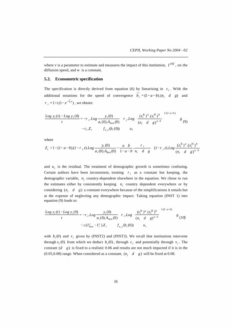
16
where v is a parameter to estimate and measures the impact of this institution, diffI , on thediffusion speed, and w is a constant.
5.2. Econometric specification
The specification is directly derived from equation (6) by linearising in ic . With the
additional notations for the speed of convergence )).(1(~
gdnba ii ++−−=β and
)1.(/1~
ti
iet βρ −−= , we obtain:
iitvii
ba
bai
bHi
aKi
ibeni
ii
ii
ubfZc
ggdn
ssLog
Aay
Logt
yLogtyLog
i++−
+
+++−=
−−−
+
))0((.
)(
).()(.
)0().0()0(
.)0()(
,
)1/(1
ρρ(9)
where
bai
bHi
aKi
ii
i
beni
iii
gdn
ssLogt
gdnbaba
Aay
LogtbaZ+++
−+++−−
+−−−−−=)(
).()()..1(.
1)0().0()0(
)..1).(1(1 ρρ
ρ
and iu is the residual. The treatment of demographic growth is sometimes confusing.
Certain authors have been inconsistent, treating iρ as a constant but keeping, the
demographic variable, in country-dependent elsewhere in the equation. We chose to run
the estimates either by consistently keeping in country dependent everywhere or by
considering )( gdni ++ a constant everywhere because of the simplifications it entails but
at the expense of neglecting any demographic impact. Taking equation (INST 1) intoequation (9) leads to:
iitvici
cben
ba
bai
bHi
aKi
ibeni
ii
ii
ubfZIIc
ggdn
ssLog
Aa
yLog
t
yLogtyLog
i++−−
+
+++−=
−−−
+
))0(()..(
)(
).()(.
)0().0(
)0(.
)0()(
,
)1/(1
ρρ(10)
with )0(ib and iv given by (INST2) and (INST3). We recall that institutions intervene
through )0(ix from which we deduct )0(ib , through ic and potentially through iv . The
constant )( gd + is fixed to a realistic 0.06 and results are not much impacted if it is in the
(0.05,0.08) range. When considered as a constant, )( gdni ++ will be fixed at 0.08.

Technology differences, institutions and economic growth :a conditional conditional convergence
17
6. RESULTS
This section starts with the estimates of the traditional Solow model and its MRWextension (6.1). In order to facilitate the understanding of the contributions of theinstitutions within the specification of equation (10) and to identify the role of educationseparately, the results are successively presented without human capital (6.2) and includinghuman capital (6.3). Then, it addresses econometric issues (6.4), provides morequantification of the role of institutions (6.5) and finally discusses the impact ofinternational trade (6.6).
6.1. Starting point estimates
Because of missing data, our sample is limited to 44 countries. As a starting point, applyingMRW approach to our data ( 0,1)0()0( === cba ii in equation (10) ), we test the
following specification:
ii
Hi
ii
Ki
iiiii ucte
dgns
Logba
bdgn
sLog
baa
yLogt
yLogtyLog++
++−−+
++−−+−=
−..
1..
1)0(.
)0()(ρρρ
An estimated b significantly different from zero distinguishes the augmented Solow modelfrom the textbook version. The speed of convergence implied by the initial incomecoefficient iρ is here )).(1(
~gdnba ii ++−−=β , lower than in the Solow model. Table II
presents the results for the Solow model in the first two columns and for the augmentedversion in the last two. Columns (2) and (4) differ from columns (1) and (3) respectively bynegating the population growth differences across countries. Disappointingly, bothspecifications have poor explanatory power when we include each country’s demographicevolution because of the restriction imposed linking the speed of convergence to individual
demographic growth.8 If we limit ourselves to columns (2) and (4), we find again the main
results of MRW, thanks econometrically to the positive correlation between initial outputand the human capital variable: the estimated physical capital share is closer to the expected(0.3-0.4) range, human capital accumulation plays a significant role, the commonempirically estimated 2% speed of convergence is consistent with the model.
< Table II >
8 Durlauf and Johnson (1995, Table II) showed that MRW sample resisted to the appropriate restriction.

CEPII, Working Paper No 2004 - 02
18
6.2. Model estimates without human capital
To incorporate the role of institutions, we start with the initial efficiency level )0(ix which
we most simply derive from the general domain of institutions, using as )0(XI either theaggregated index GENINDEX or the first factor CORRUPTION. We then infer the initialproductivity level and the pure technology component following equations (8) and(INST2). Table III gives these estimated levels, using 75.0=η . The implied initial distance
to the technological frontier is very close whether we use one indicator or the other,confirming that most of the information in this domain is included in the non-corruptionvariable. Because of the straightforward reason why corruption may induce weakefficiency, we will limit ourselves to CORRUPTIONI X =)0( from now on.
< Table III >
Institutions that most likely explain long term productivity differentials have now to bechosen. The core equation (10) is tested with cI being determined according to (INST1) bythe global index of the product and innovation domains, and the main indicator in thelabour market and financial system domains successively, keeping the rate of technologydiffusion iv constant across countries. We assess the quality of the results, summarised in
Table IV, according to three criteria: significance of the parameter estimates, explanatorypower, physical capital share estimate closer to theoretical prediction. Along these lines, theresults are very close to one another except with BANKRULES where the estimates areless precise (remember that variable definitions are found in Table I). The labour marketvariable CONTRACT is related to both limited child labour and small informal economy.Because of the very likely endogeneity of this variable, it will be dropped for furtheranalysis. The main preliminary inferences are: first, significant estimates except for thetechnological catch-up annual speed which is estimated at around 5% but is weaklysignificant, casting doubt on unconditional technology diffusion; second, institutions matterfor long term TFP-growth, in particular the global quality of the competitive productmarket and the innovation-friendly environments have a significant impact on long termgrowth entailing potential divergence; third, the explanatory power is very encouragingespecially compared to previous results shown in Table II; fourth, despite having taken intoaccount technology heterogeneity, capital share estimates are too high raising the likelihoodof misspecification and biases; sixth, and linked to the fifth, there effectively is conditionalconvergence (here it is also conditional to sharing the same technology and efficiency) at aspeed of around 3%, but too low to be in line with the underlying Solow model.
< Table IV >
As suggested in sub-section 5.1, one channel through which institutions may influencegrowth is by promoting or hindering technology diffusion. To test whether the diffusion isconditional to institutions, we use equation (INST3) taking as diffI the institutions mostlikely to do the task in the innovation domain, R&D-CAPRISK and INTPROP, andrestricting ourselves to using PRODINDEX or INNINDEX for the institution impacting
Technology differences, institutions and economic growth :a conditional conditional convergence
19
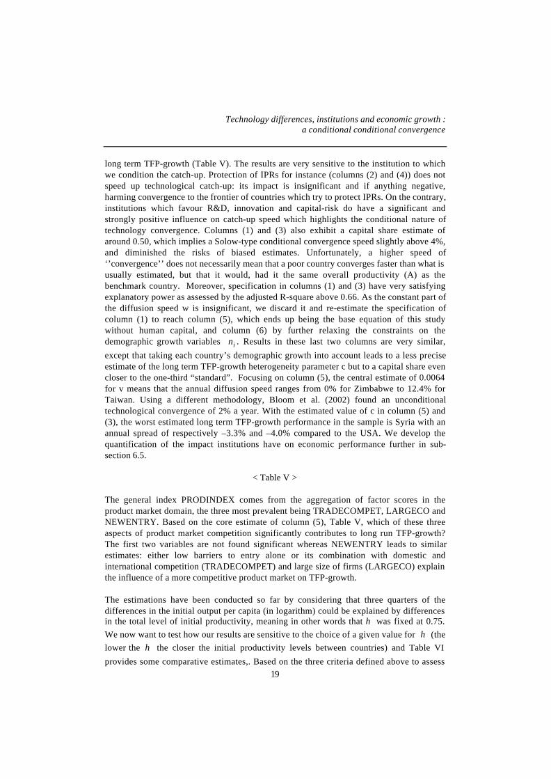
long term TFP-growth (Table V). The results are very sensitive to the institution to whichwe condition the catch-up. Protection of IPRs for instance (columns (2) and (4)) does notspeed up technological catch-up: its impact is insignificant and if anything negative,harming convergence to the frontier of countries which try to protect IPRs. On the contrary,institutions which favour R&D, innovation and capital-risk do have a significant andstrongly positive influence on catch-up speed which highlights the conditional nature oftechnology convergence. Columns (1) and (3) also exhibit a capital share estimate ofaround 0.50, which implies a Solow-type conditional convergence speed slightly above 4%,and diminished the risks of biased estimates. Unfortunately, a higher speed of‘’convergence’’ does not necessarily mean that a poor country converges faster than what isusually estimated, but that it would, had it the same overall productivity (A) as thebenchmark country. Moreover, specification in columns (1) and (3) have very satisfyingexplanatory power as assessed by the adjusted R-square above 0.66. As the constant part ofthe diffusion speed w is insignificant, we discard it and re-estimate the specification ofcolumn (1) to reach column (5), which ends up being the base equation of this studywithout human capital, and column (6) by further relaxing the constraints on thedemographic growth variables in . Results in these last two columns are very similar,
except that taking each country’s demographic growth into account leads to a less preciseestimate of the long term TFP-growth heterogeneity parameter c but to a capital share evencloser to the one-third “standard”. Focusing on column (5), the central estimate of 0.0064for v means that the annual diffusion speed ranges from 0% for Zimbabwe to 12.4% forTaiwan. Using a different methodology, Bloom et al. (2002) found an unconditionaltechnological convergence of 2% a year. With the estimated value of c in column (5) and(3), the worst estimated long term TFP-growth performance in the sample is Syria with anannual spread of respectively –3.3% and –4.0% compared to the USA. We develop thequantification of the impact institutions have on economic performance further in sub-section 6.5.
< Table V >
The general index PRODINDEX comes from the aggregation of factor scores in theproduct market domain, the three most prevalent being TRADECOMPET, LARGECO andNEWENTRY. Based on the core estimate of column (5), Table V, which of these threeaspects of product market competition significantly contributes to long run TFP-growth?The first two variables are not found significant whereas NEWENTRY leads to similarestimates: either low barriers to entry alone or its combination with domestic andinternational competition (TRADECOMPET) and large size of firms (LARGECO) explainthe influence of a more competitive product market on TFP-growth.
The estimations have been conducted so far by considering that three quarters of thedifferences in the initial output per capita (in logarithm) could be explained by differencesin the total level of initial productivity, meaning in other words that η was fixed at 0.75.We now want to test how our results are sensitive to the choice of a given value for η (thelower the η the closer the initial productivity levels between countries) and Table VI
provides some comparative estimates,. Based on the three criteria defined above to assess

CEPII, Working Paper No 2004 - 02
20
the quality of our estimates – significance, explanatory power, consistent capital share - ,the conclusions are clear-cut: allowing for productivity heterogeneity definitely improvesthe results as the estimates with the lower η is, by far, less good whatever the criteria.
Actually, columns (3 to 5) strongly support our approach, by suggesting that the share ofdifferences in initial income per capita due to the differences in total initial productivitylevels is certainly greater than one-half, which is consistent with Klenow and Rodriguez-Clare’s analysis. Moreover, these results imply that institutions matter for the efficiency inthe use of technology, approximated by a non corruption index, and omitting this impact byconsidering identical efficiency and technology is misplaced and leads to biased estimates.
< Table VI >
6.3. Human capital
Results of the previous sub-section are subject to potential biases due to omittingpotentially important variables like human capital. There are many ways in which theeducation level can influence growth. Educational achievement may have an impact on theefficiency in the use of a given technology (our iX variable), on long term TFP-growth or
on the rate of human capital accumulation. In the first two cases, the stock of humancapital, HCSTOCK, is probably the variable of interest and we use the average years ofsecond-level schooling for the population aged 25 and over in 1980 from the Barro-Leedatabase. In the third case, we will use the human capital flow variable à la MRW calledHCFLOW.
To test whether education has an influence over the efficiency level in our framework,
equation (10) is simply estimated by using HCSTOCKI iX =)0( . The results indeed suggestthat the stock of human capital at the beginning of the period is significant in explaininginitial efficiency (Table VII, column (2)). In fact, both the institutional variableCORRUPTION, a proxy for the non-corruption level, and the stock of educationHCSTOCK probably matter for efficiency. These two variables exhibit a positive linearcorrelation coefficient of 0.55 and by dichotomy we show in column (3) that the optimal
combination is achieved with HCSTOCKCORRUPTIONI iX .4)0( += .
MRW asserts that taking into account human capital as another accumulating factor enablesone to validate the Solow assumption of identical productivity across countries.9 We nowshow that the role of human capital they put forward does not conflict with our frameworkbut rather complements it. Table VIII reproduces the results where we infer that humancapital accumulation adds valuable information in the growth process without muchaltering the basic parameters estimate of section 6.1. The physical capital share estimate isnow very close to the common sense value, the joint effect of emphasising the role ofhuman capital accumulation and productivity heterogeneity.
9 Or at least uncorrelated with the regressors.

Technology differences, institutions and economic growth :a conditional conditional convergence
21
< Tables VII – VIII >
Finally, departing from the treatment of human capital as just another factor and neglectingcomplex issues of accumulation, we simply wonder if the stock of human capital has aninfluence on long term TFP-growth and therefore we include the stock measure HCSTOCKin addition to the institutional variable PRODINDEX in our ic variable. The econometrics
do show a positive contribution of human capital stock to productivity-growth and weakensomewhat the significance of our institutional variable. However, these results are doubtfulbecause the estimated physical capital share is raised back to around 70%. To summariseour results on the role of education, we find that the stock of human capital plays animportant part in explaining efficiency, quantitatively equivalent to the one coming fromother institutional variables like non-corruption (see below 6.5), and that the flow of humancapital has explanatory power in the determination of long-term growth path whichcomplements the analysis we have run so far. However the link between the stock of humancapital and the long term TFP-growth is confusing.
6.4. Econometric issues
To reach the above results we made two strong assumptions. The first is that theinstitutional quality that we measure has been deemed to be stable over the period understudy. There is not much we can do here as the information is only available for aroundyear 2000, other than betting on the robust structural dimension of these institutions.Obviously, this is an approximation as the institutional environment might have changedsignificantly for some countries between 1980 and 2000. The second issue refers to thepotential endogeneity of the institutions, and reverse causality from growth to institutionsthat may ensue. To illustrate why these concerns may not be too problematic, the R&D-CAPRISK variable, for instance, can be expected to capture an exogenous structural aspectof innovation facilitating technology transfers. Indeed, it is mainly determined by thecontribution of five items: support to R&D and innovation from the Ministry of Research,from the public or private research centres and from the technopoles (three items), thequality of the relationships between universities, research centres and companies, andfinally the importance of a financial scheme favouring capital risk. We address these pointsand check the robustness of our results in three steps. Firstly, simple descriptive statisticsreveal that our institutional variables capture deep and lasting structural components of thecountries’ characteristics. The easiest check is our non-corruption variable since othercomparable measures exist. CORRUPTION exhibits a Pearson linear correlation coefficientof 82% with Knack and Keefer’s measure for the 1980-1989 period, called here KK80-89.
10
Along those lines and with the idea of instrumenting the institutional variables that enterour core specification, CORRUPTION, PRODINDEX and R&D-CAPRISK, we regressthese three variables with potential instruments: the Knack and Keefer’s non-corruptionmeasure (KK80-89), the logarithm of output per capita in 1980 (LOGY80), the annual 10
The source is Easterly and Levine database: http://www.worldbank.org/research/growth/ddeale.htm.

CEPII, Working Paper No 2004 - 02
22
average growth rate of output per capita between 1970 and 1980 (LAGDLOGY), thefertility rate in 1980 (World Development Indicators, FERT80) and in addition thelogarithm of the investment rate Ks (LOGSK) for the PRODINDEX regression and theR&D composite indicator for 1980-1983 (World Development Indicators, R&D80-83) forthe R&D-CAPRISK regression. Despite this limited set of regressors, the high levels ofadjusted- 2R obtained (76%, 62%, 70% respectively for CORRUPTION, PRODINDEXand R&D-CAPRISK) suggest that considering these institutional variables exogenous inthe equation explaining growth between 1980 and 2000 should not be problematic.Secondly, we formally assess the endogeneity of the institutional variables for our two coreequations, with and without human capital, through a Hausman test. For the specificationwithout human capital, as we are here concerned with the endogeneity of our variables andnot with the bias coming from omitted variables (human capital), one precaution has to betaken in the choice of the instruments: human capital measures are not valid instruments asthey are most likely correlated with the residuals. Table IX presents the results withcolumns (1) and (4) being our base OLS estimates without and with human capitalrespectively – columns (1) and (4) of Table VIII. Unsurprisingly, given the econometricrelations identified above, instrumental variable estimates (IV) and OLS do not differsignificantly, even when instrumenting the investment rate variables. Hausman teststatistics imply that we should limit ourselves to the OLS. In other words, our institutionalvariables reflect robust structural components of the countries in 1980. Obviously, one canthink of cases, like China or Ireland, where rejecting endogeneity of institutions quality forgrowth estimates over the last 20 years seem dubious. However, the tests show that, in thesample overall, the deep and lasting characteristics of the institutions selected overstependogeneity concerns. Finally, another way to test the robustness of our assumptions is tocompare our estimates with estimates using a different time frame, the idea being that ifinstitutions have greatly evolved over the period, this will induce very different estimatesfor a longer period. The results, not presented here, indicate that estimates for the 1970-2000 period prove to be very close to our base results for the 1980-2000 period, whichreinforces the prospects of our institutional variables capturing structural parameters, butnon-endogeneity is not rejected as clearly as before since the Hausman test χ -square
probability is only 0.16 without human capital.
< Table IX>
The presence of outliers has also been tested. Their exclusion does not alter the main resultsand details will be provided upon requests.
6.5. Quantifying the impact of institutions further
This is beyond the scope of this study to settle the debate concerning the contribution ofhuman capital to growth as just another accumulating factor. Therefore, the followingresults are presented with the specification either without or with human capital. From thespecification without human capital, the estimated annual growth can be broken down intofour components as detailed in Appendix 3: “adjusted (to account for initial productivitylevel differences)” absolute convergence, investment rate contribution, long-term TFP-

Technology differences, institutions and economic growth :a conditional conditional convergence
23
growth and technology diffusion.11 When one takes the differences to the mean in thesample, Table X is obtained: for instance, China’s annual growth-rate over the period was4.2% above the average, the estimation of the model is 4.6%, broken down into 1.0%coming from “adjusted” absolute convergence due to decreasing capital returns, 0.5% dueto differences in investment rate, -0.8% stemming from long-term productivity-growthdifferences explained here by differences in product market efficiency detrimental to Chinaand 4.0% due to technology diffusion, the main driver of China’s over-performance.12
< Table X >
Furthermore, in order to measure the contribution of each component globally, its standarddeviation is computed and reported in Table XI. In that sense, physical capital investmentrate and technology diffusion contribute most to the differences in annual growth betweencountries having a dispersion twice as great as the one of the “adjusted” absoluteconvergence component and almost three times the one of long term TFP-growth. Whenhuman capital is included, the contribution of its accumulation rate comes third inexplaining growth dispersion across countries in between physical capital investment rateand technology diffusion on the one hand and long term TFP-growth and “adjusted”absolute convergence on the other.
Based on our estimates, we can calculate what it costs a country in terms of annual growthrate not to have the best institutions in the sample. Table XII indicates that Nigeria loses themost from the poor quality of institutions with a counterfactual growth loss of 6.1%annually, broken down into 2.3% due to poor efficiency (CORRUPTION), 2.7% because ofa weak technology diffusion (R&D-CAPRISK) and 1.1% in long term TFP-growth loss(PRODINDEX). For a comparison, Artadi and Sala-i-Martin (2003) identify eightdeterminants of Africa’s economic underperformance to OECD countries, which totals upto an annual growth deficit of around 8%. In terms of efficiency, the loss coming from aweak stock of human capital compared to the USA averages 1.3% annually, to be comparedto 0.9% for the non-corruption variable. However, the dispersions are comparable and thisis due to the over-performance of the USA in terms of education: the country that comes insecond, Japan, loses 0.6% annually to the USA because of human capital stock differences.The median annual loss over the sample due to the three major institutional aspectsidentified totals up to 2.4%. Because the sample is very heterogeneous with both countriesamong the richest and among the poorest, the institutions’ measures, resulting from the databased factor analysis, cannot differentiate much between the most developed countries, and
11
The productivity-growth component is not just ic as calculated at the end of section 6.1 - -3.3% for Syria
– but rather as apparent from equation (10) ii Zc . .
12 For the USA, 1.7 percentage point of annual growth is not accounted for by the model without human
capital. With the base estimation with human capital, USA’s growth is correctly estimated, but the USA donot appear at the technological frontier in 1980, (where Argentina and Germany stand): its initial output percapita is explained by the strong contribution of the stock of human capital to the efficiency rather than byits then technological performance. USA’s economic growth over-performance comes then from thecontribution of human capital to the steady-state and from technological catch-up.

CEPII, Working Paper No 2004 - 02
24
the counterfactual loss is calculated to be under 0.3% for the richest countries. Japan is anexception with a loss of 1.4% mainly due to a weak product market ranking. Schematically,Latin American countries suffer a loss in the 1.5%-2.5% range, North-African in the 2.5%-4%, Sub-Saharan above 4% and Asian and Eastern European are more widespread out. Theadditive average annual growth losses, over the countries in the sample, due to poor overallefficiency (as measured by CORRUPTION), to non-competitive product market(PRODINDEX) and to unfavourable environment for transferring technology (R&D-CAPRISK) are respectively 0.9%, 0.7% and 0.8%. Finally, dreaming of a world in 1980where each country would have enjoyed a quality of its institutions at the maximum overthe sample, we build Table XIII where we show different measures of inequality. Bycomparing the last two rows, we can see for instance that the world would be 52% richerand the unweighted Gini indicator would have fallen from 0.42 to 0.32 during the period,instead of the actual rise to 0.48.
< Tables XI - XII - XIII >
6.6. International trade
Appendix 4 shows that, controlling for institutions, trade does not contribute significantlyto long term TFP-growth. Trade contribution becomes significant only if exports are mostlymanufactures and the country sufficiently developed, suggesting that the impact of trade isnon-linear and depends on the specialisation of exports. As it is beyond the scope of thisstudy to overcome the issue raised by the endogeneity of trade, this last result is tentative.
7. CONCLUSION
The factor analysis of the institutional database has put forward variables that potentiallyimpact growth. Once, the role of productivity differences in the growth analysis has beenhighlighted, institutional quality is shown to matter greatly in explaining growth paths,where “convergence” appears to be not only conditional on factor accumulation rates butalso on sharing the same technology and quality of institutions. In fact, we identified thatthe growth outcome is the result of two convergent forces, decreasing returns to capital andtechnology diffusion, one divergent force, long run TFP-growth differences due toinstitutional heterogeneity, in addition to the non-convergence stemming from thedifferences in factor accumulation rates.
The greatest impacts of institutions channel through the efficiency level in the use oftechnology, well accounted for by our non-corruption variable, and through the diffusion oftechnology. Unconditional diffusion appears to be weakly significant. However, diffusion issignificantly fostered by institutions favouring R&D, innovation and capital-risk financing,whereas IPRs protection, for instance, if anything, hampers diffusion. In other respects, apro-competitive product market and an innovation-friendly environment add a significantcontribution to long run TFP-growth differences but of a lesser magnitude.
If these results are correct, they entail that development policy for the least developingcountries is necessary and should primarily target technology diffusion. International

Technology differences, institutions and economic growth :a conditional conditional convergence
25
supports should focus on countries best prepared for growth, for instance those having alow corruption index, and aim naturally at developing human capital through the health andschool systems, and also at bringing expertise to expedite the diffusion of technology andknowledge. Other measures are secondary in importance and should eventually appear at alater stage in the development process.
BIBLIOGRAPHY
Acemoglu D., P.Aghion and F.Zilibotti (2002), Distance to frontier, selection and economicgrowth, NBER Working Paper 9066.
Artadi E. and X.Sala-i-Martin (2003), The economic tragedy of the XXth century: growthin Africa, NBER Working Paper 9865.
Bassanini A. and S.Scarpetta (2001), Does human capital matter for growth in OECDcountries? Evidence from PMG estimates, OECD Working Paper 282.
Benhabib J. and M.M. Spiegel (2003), Human capital and technology diffusion, FRBSFWorking Paper 2003-02.
Benhabib J. and M.M. Spiegel (1994), The role of human capital in economic developmentEvidence from aggregate cross-country data, Journal of Monetary Economics 34(2):143-173.
Berthelier P., A.Desdoigts and J.Ould Aoudia (2003), Institutional profiles – Presentationand analysis of an original database of the institutional characteristics of developing, intransition and developed countries, Direction de la Prévision, Working Paper.
Bloom D.E., D.Canning and J.Sevilla (2002), Technological diffusion, conditionalconvergence and economic growth, NBER Working Paper 8713.
Caselli F., G.Esquivel and F.Lefort (1996), Reopening the convergence debate: a new lookat cross country growth empirics, Journal of Economic Growth 1: 363-389.
Durlauf S.N. and P.A.Johnson (1995), Multiple regimes and cross-country growthbehaviour, Journal of Applied Econometrics 10(4): 365-384.
Easterly W. and R.Levine (2002), It’s not factor accumulation: stylized facts and growthmodels, Central Bank of Chile, Working Paper 164.
Hall R.E. and C.I.Jones (1996), The productivity of nations, NBER Working Paper 5812.

CEPII, Working Paper No 2004 - 02
26
Hall R.E. and C.I.Jones (1999), Why do some countries produce so much more output perworker than others?, Quarterly Journal of Economics, February: 83-116.
Klenow P.J. and A.Rodriguez-Clare (1997), The neoclassical revival in growth economics:has it gone too far?, NBER Macroeconomics Annual 12: 73-103.
Mankiw G.N, D.Romer and D.Weil (1992), A contribution to the empirics of economicgrowth, Quarterly Journal of Economics 107: 407-437.
Nicoletti G., S.Scarpetta and O.Boylaud (1999), Summary indicators of product marketregulation with an extension to employment protection legislation, OECD WorkingPaper 226.
Pritchett L. (1997), Divergence, big time, Journal of Economic Perspectives 11(3): 3-17.
Rodrik (2003), Growth strategies, NBER Working Paper 10050.
Rodrik (2002), Feasible globalizations, NBER Working Paper 9129.
Rodrik D., A.Subramanian and F.Trebbi (2002), Institutions rule: the primacy ofinstitutions over geography and integration in economic development, NBER WorkingPaper 9305.
Temple J. (1999), The new growth evidence, Journal of Economic Literature 37(1): 112-156.

Technology differences, institutions and economic growth :a conditional conditional convergence
27
Table I: Selected institutional indicators
Domain Variable Interpretation %Variance inthe domain
General CORRUPTION Non-corruption 36%General GENINDEX Aggregated index 72%
Product market PRODINDEX Aggregated index 67%Labour market CONTRACT Limited child labour and small informal
economy26%
Financial system BANKRULES Bank control, rules, transparency 25%Innovation R&D-CAPRISK R&D effort and capital risk system 37%Innovation INTPROP Intellectual property rights 28%Innovation INNINDEX Aggregated index 77%
General FREEDOM Freedom 21%Product market TRADECOMPET Limited barriers to trade and competition
enforcement21%
Product market LARGECO Large companies in the distribution sector 25%Product market NEWENTRY Facilitation of new entry 21%Labour market UNIONFREED Trade-union rights 20%
Table II: Starting points
Solow Augmented Solow
in n=0.02in n=0.02
(1) (2) (3) (4)
a (phys.capital) 0.546(0.048)***
0.647(0.029)***
0.399(0.147)***
0.427(0.100)***
b (human capital) - - 0.163(0.152)
0.288(0.106)***
cte 0.210(0.018)***
0.173(0.013)***
0.213(0.018)***
0.162(0.014)***
Implied β 1 0.035 0.028 0.034 0.023
2R -0.05 0.31 -0.05 0.36Observations 44 44 44 44
1when taking into account the individual demographic growth, convergence speed is calculated with averagepopulation growth across countries.
(***) asymptotic significance at 99% level (**) asymptotic significance at 95% level(*) asymptotic significance at 90% level

CEPII, Working Paper No 2004 - 02
28
Table III (*): Inferred relative productivity and technology levels in 1980
GENINDEX )0(ia )0(ib CORRUPTION )0(ia )0(ibAlgeria -4.9 0.32 0.71 -4.2 0.32 0.63Argentina -0.8 0.59 0.92 -1.3 0.59 0.91Brazil 1.7 0.40 0.52 0.3 0.40 0.55Cameroon -5.1 0.17 0.39 -7.3 0.17 0.47Chile 3.2 0.35 0.42 7.4 0.35 0.33China -6.7 0.10 0.28 -1.0 0.10 0.15Colombia -0.3 0.29 0.44 -2.1 0.29 0.48Cote d'Ivoire -2.0 0.19 0.33 -6.4 0.19 0.48Egypt -8.2 0.19 0.66 -5.2 0.19 0.41France 8.6 0.81 0.75 6.7 0.81 0.79Germany 10.6 0.80 0.68 8.7 0.80 0.72Ghana -3.3 0.11 0.21 -0.7 0.11 0.16Greece 6.6 0.64 0.64 3.3 0.64 0.74Hong Kong 5.7 0.67 0.70 6.1 0.67 0.67Hungary 5.9 0.48 0.50 5.3 0.48 0.50India -1.1 0.11 0.17 -7.9 0.11 0.32Indonesia -3.4 0.16 0.30 -6.0 0.16 0.37Iran -7.5 0.28 0.88 -3.8 0.28 0.53Ireland 9.7 0.56 0.49 9.0 0.56 0.49Israel 5.8 0.62 0.65 5.8 0.62 0.63Japan 4.0 0.79 0.91 4.4 0.79 0.86Korea, Rep. 1.5 0.32 0.43 0.3 0.32 0.44Malaysia 0.0 0.32 0.48 3.3 0.32 0.37Mexico -0.6 0.45 0.70 -3.1 0.45 0.82Morocco -3.7 0.22 0.44 -0.9 0.22 0.33Nigeria -4.6 0.11 0.24 -10.2 0.11 0.49Norway 9.5 0.83 0.74 9.1 0.83 0.73Pakistan -7.3 0.11 0.33 -6.6 0.11 0.27Peru -0.4 0.32 0.49 -2.2 0.32 0.54Philippines 0.2 0.24 0.35 -4.8 0.24 0.50Poland 5.9 0.43 0.45 1.9 0.43 0.54Portugal 2.0 0.52 0.67 4.3 0.52 0.57Romania -0.3 0.17 0.26 -3.2 0.17 0.31Singapore 2.8 0.62 0.76 8.6 0.62 0.56South Africa 1.8 0.47 0.61 0.7 0.47 0.64Syria -9.5 0.22 0.99 -2.9 0.22 0.39Taiwan 1.8 0.37 0.49 3.0 0.37 0.44Thailand -2.7 0.21 0.38 -0.5 0.21 0.30Tunisia -4.2 0.30 0.62 2.7 0.30 0.36Turkey -0.1 0.29 0.43 -1.4 0.29 0.46Uganda -0.4 0.05 0.08 -4.9 0.05 0.11United States 6.8 1.00 1.00 6.3 1.00 1.00Venezuela, RB -1.4 0.47 0.77 -4.5 0.47 0.95Zimbabwe -3.9 0.20 0.41 -6.6 0.20 0.51
(*) calculations with 75.0=η

Technology differences, institutions and economic growth :a conditional conditional convergence
29
Table IV 1 : Institutions matter for long term productivity-growth
cI PRODINDEX CONTRACT BANKRULES INNINDEX
a (phys.capital) 0.624(0.088)***
0.531(0.092)***
0.619(0.075)***
0.629(0.099)***
c )( cI 0.0023(0.0012)*
0.0025(0.0008)***
0.0017(0.0011)
0.0026(0013)**
w (diffusion speed)2 2 0.053(0.033)
0.040(0.021)*
0.049(0.029)*
0.060(0.039)*
)0(benLogA 7.78(0.79)***
8.57(0.56)***
7.83(0.66)***
7.80(0.88)***
Implied β 0.030 0.032 0.021 0.0302R 0.56 0.59 0.54 0.57
Observations 44 44 44 44
1 CORRUPTIONI X =)0(
2 wv i = (v=0)
02.002.0 == ing(***) asymptotic significance at 99% level (**) asymptotic significance at 95% level(*) asymptotic significance at 90% level
Table V 1 - Conditional technology diffusion
cI PRODINDEX INNINDEX PRODIND. PRODIND.
diffI R&D-CAPRISK
INTPROP R&D-CAPRISK
INTPROP R&D-CAPRISK
R&D-CAPRISK
(1) (2) (3) (4) (5) (6)a (phys.capital) 0.484
(0.076)***0.609
(0.094)***0.502
(0.083)***0.587
(0.103)***0.483
(0.061)***0.407
(0.048)***c )( cI 0.0015
(0.0007)**0.0027
(0.0012)**0.0021
(0.0007)***0.0031
(0.0011)***0.0015
(0.0006)***0.0010
(0.0006)*
v )( diffI 2 0.0064(0.0029)**
-0.0023(0.0021)
0.0099(0.0050)**
-0.0034(0.0024)*
0.0064(0.0028)**
0.0050(0.0020)***
w 0.0002(0.0092)
0.068(0.044)*
-0.0024(0.0089)
0.081(0.050)*
- -
)0(benLogA 8.54(0.38)***
8.07(0.76)***
8.53(0.41)***
8.42(0.72)***
8.54(0.31)***
8.73(0.22)***
Implied β 0.041 0.031 0.040 0.033 0.041 0.0462R 0.66 0.58 0.68 0.61 0.67 0.66
Observ. 44 44 44 44 44 44
CORRUPTIONI X =)0(
2 wIIvv diffdiffii +−= ).( min
02.002.0 == ing except column (6) where in is unconstrained and β is calculated with averagepopulation(*** asymptotic significance at 99% level (**) asymptotic significance at 95% level(*) asymptotic significance at 90% level

CEPII, Working Paper No 2004 - 02
30
Table VI1: Productivity differences
05.0=η
(1)
5.0=η
(2)
75.0=η
(3)
1=η
(4)
25.1=η
(5)a (phys.capital) 0.642
(0.065)***0.590
(0.072)***0.483
(0.061)***0.366
(0.064)***0.233
(0.080)***
c )( cI 0.0021(0.0006)***
0.0021(0.0007)***
0.0015(0.0006)***
0.0009(0.0006)*
0.0003(0.0006)
v )( diffI 0.0205(0.1492)
0.0134(0.0113)
0.0064(0.0028)**
0.0041(0.0012)***
0.0032(0.0008)***
)0(benLogA 7.68(0.56)***
7.97(0.51)***
8.54(0.31)***
9.02(0.23)***
9.40(0.21)***
2R 0.42 0.63 0.67 0.68 0.64
Observ. 44 44 44 44 44
1 CORRUPTIONI X =)0( PRODINDEXI c = CAPRISKDRI diff −= &02.002.0 == ing
(***) asymptotic significance at 99% level (**) asymptotic significance at 95% level(*) asymptotic significance at 90% level
It can be shown that a
baaYLogVar
YLogYZLog KH η).1()1()(
),)/((cov −−−−= and therefore if, as the
intuition suggests, this covariance is positive, there is an upper bound to η which is )1/()1( baa −−− .
Table VII: Education and initial efficiency
)0(XI CORRUPTION
(1)
HCSTOCK
(2)
CORRUPTION +4.HCSTOCK
(3)a (phys.capital) 0.483
(0.061)***0.452
(0.059)***0.528
(0.065)***c )( cI 0.0015
(0.0006)***0.0021
(0.0007)***0.0019
(0.0006)***
v )( diffI 0.0064(0.0028)**
0.0042(0.0017)***
0.0073(0.0032)**
)0(benLogA 8.54(0.31)***
8.63(0.29)***
8.50(0.35)***
2R 0.67 0.66 0.70
Observ. 44 44 44

Technology differences, institutions and economic growth :a conditional conditional convergence
31
Table VIII: Education and human capital accumulation
)0(XI CORRUPTION
(1)
CORRUPTION
(2)
CORRUPTION +4.HCSTOCK
(3)
CORRUPTION +4.HCSTOCK
(4)
a (phys.capital) 0.483(0.061)***
0.302(0.091)***
0.528(0.065)***
0.361(0.093)***
b (human capital) - 0.293(0.099)***
- 0.271(0.098)***
c )( cI 0.0015(0.0006)***
0.0017(0.0008)**
0.0019(0.0006)***
0.0022(0.0009)***
v )( diffI 0.0064(0.0028)**
0.0093(0.0046)**
0.0073(0.0032)**
0.0096(0.0046)**
)0(benLogA 8.54(0.31)***
8.65(0.39)***
8.50(0.35)***
8.62(0.45)***
2R 0.67 0.72 0.70 0.74Observ. 44 44 44 44

CEPII, Working Paper No 2004 - 02
32
Table IX: Endogeneity tests
without human capital with human capital
OLS(1)
IV(2)
IV(3)
OLS(4)
IV(5)
IV(6)
a (phys.capital) 0.483(0.061)***
0.476(0.100)***
0.462(0.159)***
0.361(0.093)***
0.350(0.108)***
0.314(0.272)
b (human capital) - - - 0.271(0.098)***
0.250(0.110)**
0.236(0.250)
c )( cI 0.0015(0.0006)***
0.0024(0.0011)**
0.0025(0.0014)*
0.0022(0.0009)***
0.0025(0.0013)*
0.0029(0.0014)**
v )( diffI 0.0064(0.0028)**
0.0077(0.0067)
0.0078(0.0068)
0.0096(0.0046)**
0.0084(0.0062)
0.0081(0.0059)
)0(benLogA 8.54(0.31)***
8.69(0.49)***
8.76(0.49)***
8.62(0.45)***
8.84(0.51)***
9.12(0.76)***
Observ. 44 44 44 44 44 442R 0.67 0.65 0.64 0.74 0.73 0.70
Instruments KK80-89LOGY80
LAGDLOGY
FERT80RD80-83LOGSK
KK80-89LOGY80
LAGDLOGY
FERT80RD80-83
KK80-89LOGY80
LAGDLOGY
FERT80RD80-83LOGSKLOGSH
HCSTOCK
KK80-89LOGY80
LAGDLOGY
FERT80RD80-83
LOGSH80HCSTOCK
Hausman testStatisticPr > ChiSq
2.250.69
1.250.87
-2.761.00
-2.771.00
HeteroscedasticityWhite Statistic Pr > ChiSq
Breusch-Pagan St. Pr > ChiSq
12.00.60
2.10.35
24.90.21
3.80.15

Technology differences, institutions and economic growth :a conditional conditional convergence
33
Table X: Growth component contributions (differences to mean) (*)
annualgrowth
(1)
estimated annualgrowth
(2)
“adjusted”absolute
convergence(3)
phys. capitalinvestment rate
(4)
long termTFP-growth
(5)
techn.diffusion
(6)Algeria -1.9% -1.3% 0.0% 0.1% -0.5% -0.9%Argentina -1.9% -2.3% -0.5% 0.0% 0.0% -1.7%Brazil -1.5% 0.1% -0.2% 0.3% -0.1% 0.1%Cameroon -2.2% -2.0% 0.5% -1.9% -0.1% -0.6%Chile 1.0% -0.2% -0.1% 0.2% 0.4% -0.6%China 4.2% 4.6% 1.0% 0.5% -0.8% 4.0%Colombia -0.9% -0.8% 0.1% -0.8% -0.1% 0.0%Cote d’Iv. -3.5% -2.9% 0.4% -2.7% 0.2% -0.7%Egypt 0.7% -1.9% 0.4% -2.0% -0.1% -0.1%France -0.4% -0.3% -0.8% 1.0% 0.5% -1.0%Germany -0.2% 0.2% -0.8% 0.9% 0.7% -0.6%Ghana -1.5% -1.4% 0.9% -2.6% -0.1% 0.4%Greece -1.0% -0.2% -0.6% 0.7% 0.6% -0.9%Hong Kong 1.7% 0.4% -0.6% 1.2% 0.4% -0.5%Hungary -0.8% 0.9% -0.4% 0.3% 0.6% 0.3%India 1.8% 0.9% 0.9% -0.8% -0.3% 1.1%Indonesia 1.2% 0.6% 0.6% 0.1% -0.4% 0.3%Iran -0.1% -1.3% 0.1% 0.5% -1.3% -0.7%Ireland 2.8% 1.3% -0.5% 0.5% 0.7% 0.5%Israel -0.1% 0.7% -0.6% 1.1% 0.4% -0.2%Japan 0.2% -0.7% -0.8% 1.8% -0.2% -1.4%Korea, Rep. 3.9% 2.7% 0.0% 2.0% -0.3% 1.0%Malaysia 1.5% 2.2% 0.0% 1.1% -0.3% 1.5%Mexico -1.4% -1.7% -0.3% 0.3% 0.1% -1.7%Morocco -1.0% 0.7% 0.3% -0.6% -0.1% 1.1%Nigeria -4.7% -2.5% 0.9% -1.7% -0.3% -1.3%Norway 0.3% 0.5% -0.8% 1.6% 0.5% -0.7%Pakistan 0.7% 1.6% 0.9% -0.9% -0.1% 1.7%Peru -2.3% -0.7% 0.0% 0.3% 0.1% -1.1%Philippines -1.8% -0.3% 0.2% -0.2% -0.2% -0.1%Poland -0.7% 0.7% -0.3% 0.5% 0.2% 0.2%Portugal 0.8% 0.7% -0.4% 0.8% 0.5% -0.2%Romania 1.4% 2.2% 0.5% 0.8% -0.2% 1.1%Singapore 2.8% 2.8% -0.6% 2.6% 0.5% 0.3%South Afr. -2.2% -2.1% -0.3% -1.4% 0.2% -0.6%Syria -0.5% -1.2% 0.3% -0.9% -1.0% 0.4%Taiwan 3.9% 1.7% -0.1% 0.5% 0.1% 1.3%Thailand 2.6% 2.9% 0.3% 1.7% -0.5% 1.4%Tunisia 0.2% 1.3% 0.0% -0.3% 0.0% 1.6%Turkey 0.3% 0.3% 0.1% 0.1% 0.0% 0.1%Uganda 1.7% 0.2% 1.5% -4.6% 0.3% 3.0%United States 0.2% -1.5% -1.0% 0.6% 0.7% -1.9%Venezuela -3.0% -2.7% -0.3% -0.3% -0.2% -1.8%Zimbabwe -2.2% -2.3% 0.4% -0.5% -0.3% -1.9%
(*) The estimated annual growth difference to the mean in column (2) is the sum of the four contributions incolumns (3 to 6).
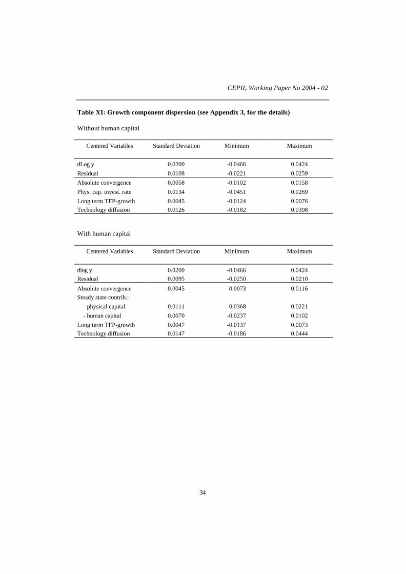
CEPII, Working Paper No 2004 - 02
34
Table XI: Growth component dispersion (see Appendix 3, for the details)
Without human capital
Centered Variables Standard Deviation Minimum Maximum
dLog y 0.0200 -0.0466 0.0424Residual 0.0108 -0.0221 0.0259Absolute convergence 0.0058 -0.0102 0.0158Phys. cap. invest. rate 0.0134 -0.0451 0.0269Long term TFP-growth 0.0045 -0.0124 0.0076Technology diffusion 0.0126 -0.0182 0.0398
With human capital
Centered Variables Standard Deviation Minimum Maximum
dlog y 0.0200 -0.0466 0.0424Residual 0.0095 -0.0250 0.0210
Absolute convergence 0.0045 -0.0073 0.0116Steady state contrib.: - physical capital 0.0111 -0.0368 0.0221 - human capital 0.0070 -0.0237 0.0102Long term TFP-growth 0.0047 -0.0137 0.0073Technology diffusion 0.0147 -0.0186 0.0444

Technology differences, institutions and economic growth :a conditional conditional convergence
35
Table XII: Deficit in annual growth rate due to poor institutional quality 1980-2000(model with human capital)
Total CORRUPTION R&D-CAPRISK PRODINDEX To compare:Stock of humancapital
Nigeria 6.1% 2.3% 2.7% 1.1% 2.3%Zimbabwe 5.4% 1.7% 2.4% 1.3% 1.9%Ghana 5.2% 1.0% 3.4% 0.8% 1.6%Iran, Islamic Rep. 4.3% 1.0% 0.9% 2.4% 1.3%India 4.3% 1.9% 1.1% 1.3% 1.9%Indonesia 4.1% 1.6% 1.2% 1.3% 1.8%Cameroon 4.0% 1.8% 1.5% 0.7% 2.0%Syrian ArabRepublic 4.0% 1.0% 0.9% 2.1% 1.3%Uganda 3.9% 2.0% 1.7% 0.2% 2.5%Egypt, Arab Rep. 3.9% 1.4% 1.4% 1.1% 1.6%Cote d'Ivoire 3.5% 1.7% 1.4% 0.4% 1.9%Pakistan 3.5% 1.8% 0.9% 0.8% 1.9%Romania 3.4% 1.1% 1.1% 1.2% 1.4%Algeria 3.2% 1.2% 0.5% 1.5% 1.6%Philippines 3.2% 1.2% 0.8% 1.2% 1.3%Peru 3.1% 0.9% 1.4% 0.8% 1.2%China 3.1% 1.0% 0.2% 1.9% 1.5%Thailand 2.9% 0.9% 0.7% 1.3% 1.5%Chile 2.8% 0.1% 2.3% 0.4% 0.9%Morocco 2.5% 1.0% 0.6% 0.9% 1.6%Turkey 2.5% 1.0% 0.7% 0.8% 1.4%Colombia 2.4% 0.9% 0.6% 0.9% 1.3%Mexico 2.3% 1.1% 0.4% 0.8% 1.4%Venezuela, RB 2.2% 1.1% 0.2% 0.9% 1.2%Korea, Rep. 2.0% 0.6% 0.1% 1.3% 0.8%Malaysia 1.9% 0.4% 0.2% 1.3% 1.0%Brazil 1.8% 0.7% 0.2% 0.9% 1.3%Tunisia 1.6% 0.5% 0.2% 0.9% 1.3%Argentina 1.5% 0.8% 0.0% 0.7% 1.1%South Africa 1.5% 0.7% 0.2% 0.6% 1.2%Japan 1.4% 0.3% 0.0% 1.1% 0.6%Taiwan 1.3% 0.5% 0.0% 0.8% 0.9%Poland 1.2% 0.5% 0.2% 0.5% 1.0%Portugal 0.9% 0.4% 0.2% 0.3% 1.1%Hungary 0.7% 0.3% 0.2% 0.2% 1.1%Hong Kong, China 0.7% 0.2% 0.1% 0.4% 0.6%Israel 0.6% 0.2% 0.0% 0.4% 0.7%Greece 0.5% 0.4% 0.0% 0.1% 1.0%France 0.5% 0.2% 0.0% 0.3% 0.8%Singapore 0.3% 0.0% 0.0% 0.3% 1.0%Norway 0.3% 0.0% 0.0% 0.3% 0.7%United States 0.2% 0.1% 0.0% 0.1% 0.0%Ireland 0.2% 0.0% 0.2% 0.0% 0.7%Germany 0.1% 0.0% 0.0% 0.1% 1.0%
mean 2.4% 0.9% 0.7% 0.8% 1.3%std 1.6% 0.6% 0.8% 0.5% 0.5%

CEPII, Working Paper No 2004 - 02
36
Table XIII: A brave new world: Inequality of income per capita ($ PPP)
Time Institutions Mean Standard Dev. Variation Coeff. Gini
1980 actual 6500 5100 0.78 0.422000 actual 9750 8600 0.88 0.482000 best 14850 7950 0.54 0.32

Technology differences, institutions and economic growth :a conditional conditional convergence
37
Chart 1: GDP per capita and (non-)corruption index
ALG
ARG
BRA
CAM
CHL
COTEGY
FRA
GER
GHA
GRE
HKOHUN
IND
INO
IRA
IRE
ISR
JAP
KOR
MAL
MEX
MOR
NIG
PAK
PER
PHI
POL
POR
ROM
SIN
SOA
SYR
TAI
THA
TUN
UGA
USA
VEN
CHNCOL
NOR
TUR
ZIM
-3 -2 -1 0 1 2Log (GDP/capita in 1980, PPP)
CO
RR
UP
TIO
N
Chart 2: R&D-CAPRISK and PRODINDEX
ALG
ARG BRA
CAM
CHL
CHN
COL
EGY
FRA
GER
GHA
GRE
HKO
HUN
INDINO
IRA
IRE
ISR
JAP KORMAL
MEX
MOR
NIG
PAK
PER
PHI
POL
POR SIN
SOA
SYR
TAI
TUNTUR
USA
ZIM
COT
NOR
ROM
THA
UGA
VEN
-10 -5 0 5 10 15R&D-CAPRISK
PR
OD
IND
EX

CEPII, Working Paper No 2004 - 02
38
APPENDIX 1: The growth equation
The productivity growth of country i at time t, )(tg i is given by equation (5):
))0(1(
))0(1.()()(
.i
tvii
ii
ii
be
bvcgt
AA
tgi −−
−+−=≡
&(A1)
and under the assumption that, in the long run, there is technological convergence to the
frontier ( 0≥iv ) :
*)(lim iiit
gcgtg ≡−=∞→
and we note ))0(1(
))0(1.()()(
.*
itv
iiiii
be
bvgtgt
i −−
−=−≡γ
Using notation of equation (7) in the main text, equation (A1) has the following solution:
tfgii
tvieAtA ).( ,*
).0()( += (A2)
It is common to work with the quantity of capital and output per unit of effective labour,
ii LA . ,
)./(~)./(
~)./(
~
iiii
iiii
iiii
LAYy
LAHh
LAKk
≡
≡
≡
(A3)
From the dynamic of physical capital, we derive the dynamic of ik~
:
iKiiiii yskdgnk ~.
~).(
~+++−=&
(A4a)
and equivalently for human capital.
iHiiiii yshdgnh ~.
~).(
~+++−=&
(A4b)
Therefore, one can show as in MRW that the steady-state levels are:
)1/(1**
)1/(1*1*
)1/(1*1*
))/().()((~))/().()((
~))/().()((
~
babaii
bHi
aKii
baii
aHi
aKii
baii
bHi
bKii
dgnssy
dgnssh
dgnssk
−−+
−−−
−−−
++=
++=
++=
(A5)
It follows from (A4a-b):
)().())(~~
..())(~~
..(~
~.~
~.~
~** tbadgn
h
ysbdgn
k
ysa
h
hb
k
ka
yy
iiii
iHiii
i
iKi
i
i
i
i
i
i γ+−++−+++−=+=&&&

Technology differences, institutions and economic growth :a conditional conditional convergence
39
Log-linearising around the steady-state, with the rate of
convergence )).(1( * dgnba iii ++−−=β , and using the expression in A(5) leads to:
)().()~~.(
)().()~~
~~
).(.()~~
~~
).(.(~
~~
*
*
**
*
**
tbayLogyLog
tbah
yLog
h
yLogdgnb
k
yLog
k
yLogdgna
yy
dtydLog
iiii
ii
i
i
iii
i
i
i
iii
i
ii
γβ
γ
+−−−=
+−−+++−++==&
(A6)
overestimate the growth of both physical and human capital per unit of effective labour.
The solution to the differential equation (A6) is:
∫−− +−−=−t
ixt
iit
ii dxxeebayLogyLogeyLogyLog iii
0
..*.* ).(..).()~)0(~.(~~ γβββ (A6)
By using the steady-state expression given by (A5), and noting
∫−+≡t
ixt
tv dxxet
eba ii
0
.., ).(..
1.).( γγ ββ , (A6) becomes the growth equation :
tv
ba
baii
bHi
aKi
iiiii
cgdn
ssLogyLog
tyLogtyLog
,
)1/(1
)(
).()(.)0(~.
)0(~)(~γρρ −
−+++−=
−−−
+
with )1.(/1 ti
iet βρ −−=
Output per worker is easily derived from output per effective labour by using equation(A2):
tvtvi
ba
baii
bHi
aKi
ii
ii
ii fcgcgdn
ssLog
Ay
Logt
yLogtyLog,,
)1/(1
)().()(
.)0()0(
.)0()(
γρρ −+−+
−+++−=
−−−
+
The specification of equation (6) is then established by neglecting tv ,γ compared to tvf , .
Based on simulations, the following Table gives an order of the magnitude of thisapproximation. The lower the physical and human capital share the more legitimate theapproximation is. Actually, the important thing to notice is that both tvf , and tvh , increase
with the rate of technological diffusion. Given capital shares, as the ratio of theapproximation (last column) is stable over the countries (different )0(ib , see the first three
lines), specification of equation (6), which neglects tv ,γ , simply means that the rate of
diffusion is somewhat underestimated, the more so that capital shares are high.

CEPII, Working Paper No 2004 - 02
40
iv a+b )0(ib tvf , tv ,γ
tv
tvtv
f
f
,
,, γ−
5% 0.35 0.25 5.35% 0.98% 0.825% 0.35 0.50 2.45% 0.47% 0.815% 0.35 0.75 0.96% 0.19% 0.805% 0.60 0.50 2.45% 1.01% 0.591% 0.35 0.50 0.83% 0.18% 0.7910% 0.35 0.50 3.12% 0.55% 0.82

Technology differences, institutions and economic growth :a conditional conditional convergence
41
APPENDIX 2: Factor analysis
1. Defining five domains and redressing two values
The 94 indicators (see section 4.2) were clustered into 5 domains: product market, labourmarket, financial market, innovation and a general heading for all other items, eachrepresenting a specific aspect of a country‘s institutions. Table A1 gives the breakdown ofthe indicators. Each indicator is defined in a (0;4) range. A descriptive statistical analysisleads to redress two indicator values for the USA. In the general domain, the indicator B300(“Collusion between the State and firms”) takes the value of 1.5 for the USA whereas, forinstance for OECD countries, France and Germany take a 4, Japan a 2.5. We decided toredress the USA notation to a conservative 3. In the product market domain, indicator B704(“Pressure on competition from employer organisations”) shows: USA 1, Greece 4, Franceand Germany 3. We redressed the value for the USA to 3.
2. Factor analysis methodology
For each domain, we run a factor analysis in covariance which provides a more informativestatistical summary. Within a given domain, the underlying factors are constructed as alinear combination of the indicators in the domain, in such a way that these factors retainthe most information as measured by the cross-country variance. We aim at identifying themain factors with sub-domains which would be meaningful in economic terms. Themethodology is very close to Nicoletti, Scarpetta and Boylaud (1999) who calculateindicators for Product Market Regulation in OECD countries. For each domain, we validateour approach by a chi-squared significance test (Bartlett test) and we select the number offactors based on Akaike’s information criterion and Schwarz’s bayesian criterion. Once theoptimal dimension of the projection space has been deduced, we use the varimax method torotate the axes in order to minimise the number of variables with high absolute loadings oneach factor, so that factor interpretation is facilitated. Each country has then a score on eachrotated factor. From factor scores, an aggregated index is calculated (for each domain).Here the aggregation procedure differs somewhat from Nicoletti et al.’s. The aggregationdetails are given below.
We use matrix algebra. For a given domain, )],([ jixX = is the original data with i
indexing the countries from 1 to I, and j indexing the primary indicators in the domain from1 to J. The factor scores matrix is )],([ kizZ = where k indexes the rotated factors from 1
to K, K being the number selected factors. By denoting )],([ kjvV = the matrix of the K
normalised eigen vectors, the factor analysis algebra is written:
LZVar
VXZ
=
= .

CEPII, Working Paper No 2004 - 02
42
where L is the (K,K) diagonal matrix with the k-th coordinate being the eigen value kl .
Before calculating the aggregated index, we project orthogonally the variables jX in the
factors space Z and obtain the estimated X̂ as follows:
''1''1'1' ..........).(ˆ VZVLLVXXXVLVXXZZZZX ==== −−−
As we chose to rotate the axes, what makes sense for the aggregated index is only theoverall information in the factor space not on each factor individually. A variable jX
which is a 100% in the factor space will be left intact by the transformation from jX to
jX̂ whereas a variable 'jX orthogonal to the factor space will disappear. We then define
our aggregated index as the average of the transformed variables.
JJ VZKXKINDEX 1../11.ˆ/1 '==
where J1 is the (J,1) vector of coordinate j equals to 1. Developing the matrix formula
above leads to:
=
=
∑ ∑
∑∑ ∑∑ ∑
=
==
K
k jjk
jijjk
K
k jjk
K
k jjkik
i
v
xvv
K
vz
INDEX
1
2
11..
This aggregated measure is appealing because it is directly based on the factor scores, i.e.the sub-domain indicators, each being weighted using the coordinates of the correspondingeigen vector. It is close to Nicoletti et al’s aggregated indicator which is computed asfollows:
∑∑∑=
=
jijjk
K
kk
k
kNSB xv
ll
INDEX .. 2
1
The interesting property of our aggregated indicator is the consistency with the choice ofrotating the axes. Indeed, it is easily shown that this indicator is invariant to an orthogonalrotation of the factor space. If T is one of these orthogonal transformation, characterised by
KITT =.' , the K-dimension identity matrix, then the eigen vectors become TVV .~ = and
the index is left unchanged:
INDEXVVXKVVXKEXDIN JJ === 1.../11.~.~./1~ ''

Technology differences, institutions and economic growth :a conditional conditional convergence
43
3. Results
Results are presented for each domain. Tables A show the tests and the eigen valuesbreakdown. Tables B refer to the factor interpretation, i.e. sub-domain identification,highlighting the variables which contribute most to the variance. Tables C contain the sub-domain indicators (i.e. the factor scores) and the aggregated index. All these indicators arenormalised so that they are centered and their standard deviation equals 5.
3.1 General domain (GEN)
The tests described above lead us to select four factors for the general domain, but the firsttwo together contribute to 57% of the variance, whereas the last two to only 16%.Moreover, the interpretation of factors 3 and 4 are not obvious. The first factor,CORRUPTION, is clearly an indicator of non-corruption; it ranges from 9.1 for Norwaydown to –10.2 for Nigeria. The second factor, FREEDOM, is determined by a set ofprimary indicators referring to different aspects of freedom. The aggregated index,GENINDEX, based on these four factor-scores ranges from 10.6 for Germany to –9.5 forSyria.
3.2 Product market domain (PROD)
The product market domain can be limited to three sub-domains that explain 67% of thevariance. Each sub-domain is easily identified and contributes to roughly a third of thecross-country information within the domain. These are: TRADECOMPET , an indicator ofthe limited restrictions to imports, of the enforcement of international trade rules, forinstance through membership to the WTO, and of competition regulation to avoid collusionand abuse of market power; LARGECO, the share of large companies in the distributionsector which is possibly a broader indicator of firm size and efficient scale, NEWENTRY,barriers to new entry.
3.3 Labour market domain (LABR)
Four factors are necessary in the labour market domain. The first one, CONTRACT, onlycontributes to more than 20% of the variance. It refers to the weak contributions of childlabour and informal economy, which is indeed an important characteristic as the samplefocuses primarily on developing countries. The second, UNIONFREED, an indicator oftrade-union freedom, accounts for roughly 20% of the variance. The last two have acontribution of only 11% and are representative of labour flexibility and unemploymentamong the skilled young. The general index LABRINDEX is a mixture of components thatwe generally tend to oppose to each-other, like strong unions and labour flexibility.Therefore, it is not easily readable and will be dropped from the analysis.

CEPII, Working Paper No 2004 - 02
44
3.4 Bank and Financial system (FIN)
This domain is the more difficult to interpret. Although only two factors contribute to 20%or more, tests require five factors. The first one, BANRULES, has a clear-cut interpretation,referring to banking regulation and prudential rules, and contributes to around 25% of theoverall variance in the domain. The second rotated factor, DEPGUARANT, is mostlyexplained by item C602 which is a dummy variable identifying countries where there is alaw by which the State guarantees deposits. It is fairly dubious. Three other domains areidentified but they each represent 10% or less of total variance. These are domestic andinternational competition in the financial system, credit access, and, more tentatively,debtor protection. Here also, the general index is fairly intangible and therefore we willlimit ourselves to BANKRULES.
3.5 Innovation domain (INN)
Factor analysis in this domain clearly identifies three distinct aspects linked to theinnovation environment. The first sub-domain, R&D-CAPRISK, has in fact a doublecomponent: on the one hand, efforts to promote R&D and innovation, and on the other, asystem favouring capital risk financing. It contributes 37% of the variance. The second sub-domain, INTPROP, refers to the protection of intellectual property rights and, to a lesserextent, to a developed environment of insurance companies and pension funds. It also has astrong contribution of 28%. The third sub-domain, PROP, is more broadly linked to theprotection of property rights but contributes to only 12.5% of the domain variance.
3.6 Correlation
The computation of linear Pearson coefficients between the aggregated indices of eachdomain reveals a strong correlation. Table A2 shows that linear correlation coefficientsrange from 0.67 to 0.88. This entails that if we want to capture a specific aspect ofinstitutions, we should lean towards focusing on less aggregated data as much as possible,like the identified factors themselves. In other words, we have to carefully weigh the trade-off between greater variance and more detailed information.

Technology differences, institutions and economic growth :a conditional conditional convergence
45
APPENDIX 3: Components of the growth equation
The specification without human capital is taken as an example. It is easily extended whenhuman capital is included. From equation (10) in the main text, we derive four componentsof estimated growth. The first is the “adjusted” absolute convergence term. The typical termis lessened here because of differences in initial productivity level. The second is theinvestment rate contribution through its influence on the steady-state. The third refers to thedynamic efficiency loss due to the institution )0(XI . It does not capture the whole long termTFP-growth term icg − because of the transitional dynamics. To understand this, keep in
mind that the usual first two terms above take into account the individual TFP-growth. It isthe total effect of having a lower persistent TFP-growth that is reflected in the variable iZand taken into account in this third term. The last component of growth is a transitionalcontribution coming from technological diffusion. Formally, using equation (10):
)0()).0(1(1
.1log
)..(
..1
)0().0()0(
.""
.
i
tvi
ici
cben
i
ii
beni
ii
beb
Logt
diffusionicaltechno
ZIIcggrowthTFPtermlong
dgns
Loga
arateinvestment
Aay
Logeconvergencabsoluteadjusted
i−−−=
−−=−
++−=
−=
ρ
ρ
To calculate what it costs a country not to have perfect institutions as it is reported in TableXII, we assess counterfactually what would be its estimated growth with 1)0( =ix ,
diffdiffi II max= and c
benci II = . As there is a cross term in the iZ expression, we split them
equally between the two institutional variables. Formally,
))0(().2/.1).(1.(.)(
)).0(1(1
)).0(1(1.
1)(
))0(()).2/.1).(1.(()(
)..(
)..(
)0(
min
minmax
iiiiic
tIIvi
tIIvidiff
iiiiX
xLogtacZcIimpact
eb
ebLog
tIimpact
xLogtacIimpact
diffdiffi
diffdiff
ρ
ρρ
−−−=
−−
−−=
−−−−=
−−
−−

CEPII, Working Paper No 2004 - 02
46
APPENDIX 4: Trade contribution
It is beyond the scope of this study to overcome the issue raised by the endogeneity of tradein its contribution to growth. Recognising this limitation, we will nevertheless show someresults hoping they shed some light on the complex mechanism at work. Static gains fromtrade spread over a transition period or dynamic gains from spillovers should result, at leasttemporarily, in increased total productivity. If we use as a trade variable the sum of exportsplus imports divided by GDP (OPENC in the Penn World Table), take the average over theperiod and add it into (INST1) to test the impact of openness over TFP-growth using
).().( max ici
cbeni TradeTradedIIcc −+−= (INST1’)
the sensitivity of growth to trade, as measured by the parameter d, is found to beinsignificant. More trade does not seem to expedite growth. However, we found twosignificant different contributions of trade. The first is obtained when crossing the opennesslevel with the percentage of manufactures exports in total exports (World DevelopmentIndicators). The intuition refers to the idea that trade in agriculture or raw materials may notbe beneficial at all in terms of TFP-growth. Table A4 shows, starting in column (1) fromour base estimate from Table V column (5), our new estimates when we include trade asopenness ratio in column (2) and when we cross it with the manufacturing export share incolumn (3).13 With the average estimate of 0.0212 for d, a country like Hungary with64.5% of its exports being manufactured products is expected to add 0.27% annually tolong term growth-rate when its exports and imports each increase by 10% of GDP whereasmost of Sub-Saharan countries will add virtually nothing. We obviously did not go furtherinto sector details, but this result suggests either that specialisation matters for the impact oftrade on growth or that, if we take the manufacturing share in exports as a developmentindicator, trade is important for efficiency later on in the development phase. The secondsignificant contribution of trade we obtained reinforces these inferences. Going one stepfurther and crossing the trade variable of column (3) with dummy variables which separatethe sample into two, with the break point at average initial income per capita, we concludethat exporting manufactures (as a share of GDP) increases growth for relatively richcountries only (column 4), the effect being insignificant – or if anything negative – for poorcountries (column 5). We deduce, echoing Acemoglu, Aghion and Zilibotti (2002) that thepositive effect of (specialised) trade on growth is non linear with liberalising to trade nothelping much in the early stage of development. The magnitude of the contributionmeasured by the dispersion as in Tables XI points to a standard deviation of the tradecontribution of 0.25%, 0.35% and 0.50% for specification in columns (2), (3) and (4)respectively, equivalent to the one identified for product market competition level which bythe way, becomes less significant as trade does. We also tested whether increased tradeaccelerates the speed of technology diffusion through an increased speed and found nosignificant impact. Finally, testing the impact of trade through the more thorough
13
Our openness measures is the OPENC average of years 1980, 1990 and 1995 - chosen because of missing datafor 2000 - capped at 100% to avoid some awkward effects coming for example from extreme case like Singaporewith openness level over 400%. Not capping tends to flatten out the impact and probably leads to less relevantresults.

Technology differences, institutions and economic growth :a conditional conditional convergence
47
specification including human capital leads to similar estimates. Although we acknowledgethe limitations described above due to the endogeneity issue, this result conflicts with those(more rigorous) of Easterly and Levine (2002) and Rodrik, Subramanian and Trebbi (2002).
< Table A4 >
Table A4: Trade contribution to growth
TRADE VARIABLE - Openness Openness *Manufacturesexport share
Openness *Manufacturesexport share *
Dummy ‘’rich’’
Openness *Manufacturesexport share *
Dummy ‘’poor’’(1) (2) (3) (4) (5)
a (phys.capital) 0.484(0.076)***
0.483(0.063)***
0.442(0.075)***
0.466(0.079)***
0.462(0.054)***
c )( cI 0.0015(0.0007)**
0.0015(0.0007)**
0.0008(0.0006)*
0.0006(0.0006)
0.0016(0.0007)**
v )( diffI 0.0064(0.0029)**
0.0063(0.0029)**
0.0048(0.0021)**
0.0071(0.0031)**
0.0079(0.0038)**
d (Trade) - 0.003(0.013)
0.021(0.012)**
0.027(0.011)***
- 0.033(0.030)
)0(benLogA 8.54(0.38)***
8.57(0.34)***
8.98(0.40)***
8.89(0.38)***
8.23(0.37)***
2R 0.67 0.66 0.68 0.70 0.67
Observ. 44 44 44 44 44
Table A2: Pearson Correlation Coefficients, N = 51
genindex prodindex labrindex finindex innindexgenindex 1.000 0.884 0.819 0.832 0.881
prodindex 0.884 1.000 0.748 0.846 0.875
labrindex 0.819 0.748 1.000 0.667 0.693
finindex 0.832 0.846 0.667 1.000 0.845
innindex 0.881 0.875 0.693 0.845 1.000
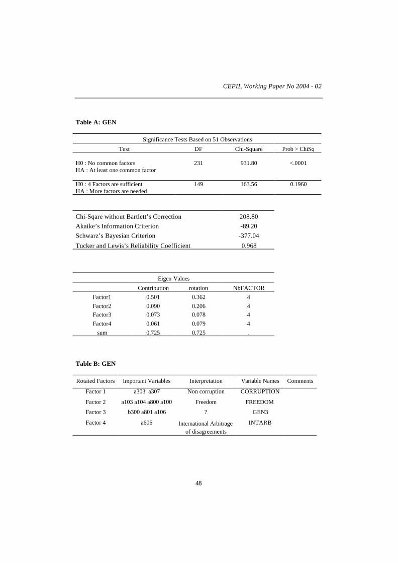
CEPII, Working Paper No 2004 - 02
48
Table A: GEN
Significance Tests Based on 51 Observations
Test DF Chi-Square Prob > ChiSq
H0 : No common factorsHA : At least one common factor
231 931.80 <.0001
H0 : 4 Factors are sufficientHA : More factors are needed
149 163.56 0.1960
Chi-Sqare without Bartlett’s Correction 208.80Akaike’s Information Criterion -89.20Schwarz’s Bayesian Criterion -377.04
Tucker and Lewis’s Reliability Coefficient 0.968
Eigen Values
Contribution rotation NbFACTORFactor1 0.501 0.362 4Factor2 0.090 0.206 4Factor3 0.073 0.078 4Factor4 0.061 0.079 4
sum 0.725 0.725 .
Table B: GEN
Rotated Factors Important Variables Interpretation Variable Names Comments
Factor 1 a303 a307 Non corruption CORRUPTION
Factor 2 a103 a104 a800 a100 Freedom FREEDOM
Factor 3 b300 a801 a106 ? GEN3
Factor 4 a606 International Arbitrageof disagreements
INTARB

Technology differences, institutions and economic growth :a conditional conditional convergence
49
Table C: GEN
CORRUPTION FREEDOM GEN3 INTARB GENINDEXAlgeria -4.2 -5.6 2.7 4.9 -4.9Argentina -1.3 0.3 -3.4 3.9 -0.8Bulgaria 0.3 4.2 -3.4 -1.0 1.7Brazil 1.0 2.4 -6.4 -3.1 0.1Cameroon -7.3 1.1 3.0 -3.8 -5.1Chile 7.4 0.0 -3.4 -9.0 3.2China -1.0 -10.5 -4.2 4.2 -6.7Colombia -2.1 0.9 -1.4 5.7 -0.3Ivory Coast -6.4 2.9 1.2 4.8 -2.0Czech Republic 1.4 4.1 -1.7 -3.7 2.3Egypt -5.2 -8.6 2.1 1.0 -8.2France 6.7 2.0 6.2 4.8 8.6Germany 8.7 2.2 8.5 3.7 10.6Ghana -0.7 0.7 -2.2 -13.3 -3.3Greece 3.3 4.0 9.4 -1.3 6.6Hong Kong 6.1 -0.3 -2.1 8.2 5.7Hungary 5.3 2.2 -2.6 5.9 5.9India -7.9 5.9 6.3 1.6 -1.1Indonesia -6.0 3.4 1.6 -5.3 -3.4Iran -3.8 -6.9 -0.2 -3.2 -7.5Ireland 9.0 2.6 6.8 -0.7 9.7Israel 5.8 -1.4 3.4 6.8 5.8Japan 4.4 3.8 -4.9 -2.6 4.0Korea, Rep. 0.3 4.9 -9.1 2.3 1.5Lithuania 4.5 5.9 -14.2 7.4 5.2Malaysia 3.3 -6.1 2.6 1.4 0.0Mexico -3.1 3.2 0.6 -0.4 -0.6Morocco -0.9 -2.8 -4.1 -2.7 -3.7Nigeria -10.2 4.3 3.5 0.6 -4.6Norway 9.1 2.1 3.1 3.1 9.5Pakistan -6.6 -2.6 0.1 -4.2 -7.3Peru -2.2 0.8 1.2 3.0 -0.4Philippines -4.8 4.7 1.2 4.5 0.2Poland 1.9 4.9 3.2 4.9 5.9Portugal 4.3 4.8 -9.0 -10.6 2.0Romania -3.2 2.7 -1.1 4.2 -0.3Russia -2.5 0.8 -0.2 -1.1 -1.7Saudi Arabia 2.9 -15.9 3.4 -0.4 -6.1Singapore 8.6 -7.9 0.4 2.7 2.8South Africa 0.7 1.3 7.4 -5.3 1.8Syria -2.9 -10.7 -3.8 -2.0 -9.5Taiwan 3.0 3.6 0.3 -13.0 1.8Thailand -0.5 -2.0 -9.4 4.4 -2.7Tunisia 2.7 -9.2 -0.2 -5.3 -4.2Turkey -1.4 0.0 4.2 0.3 -0.1Ukraine -4.9 4.6 4.3 -0.4 -0.4Uganda -4.6 0.6 -8.1 1.6 -4.6United States 6.3 3.0 6.4 -6.0 6.8Venezuela, RB -4.5 2.8 -2.2 4.6 -1.4Vietnam -2.3 -6.7 -2.2 -2.8 -6.5Zimbabwe -6.6 -0.8 6.7 0.8 -3.9

CEPII, Working Paper No 2004 - 02
50
Table A: PROD
Significance Tests Based on 51 Observations
Test DF Chi-Square Prob > ChiSq
H0 : No common factorsHA : At least one common factor
91 383.90 <.0001
H0 : 3 Factors are sufficientHA : More factors are needed
52 55.13 0.3573
Chi-Sqare without Bartlett’s Correction 64.85Akaike’s Information Criterion -39.14Schwarz’s Bayesian Criterion -139.60Tucker and Lewis’s Reliability Coeeficient 0.9813
Eigen ValuesContribution Rotation NbFACTOR
Factor1 0.499 0.214 3Factor2 0.092 0.252 3Factor3 0.083 0.207 3
sum 0.673 0.673 .
Table B: PROD
Rotated Factors ImportantVariables
Interpretation Variable Names Comments
Factor 1 B8020 a701b800 b801
Few barriers to imports,international trade rules(WTO) and competitionenforcement
TRADECOMPET Strong negativecoordinate of b702which contributesgreatly to factor2
Factor 2 B702 Large companies in thedistribution sector
LARGECO
Factor 3 B301 b700 Enhancement of newfrims
NEWENTRY To a lesser extent:b601, quality norms

Technology differences, institutions and economic growth :a conditional conditional convergence
51
Table C: PROD
TRADECOMPET LARGECO NEWENTRY PRODINDEXAlgeria -0.9 -5.6 -3.1 -5.0Argentina -2.5 3.0 1.2 0.3Bulgaria -2.2 3.9 -1.9 -0.3Brazil -4.7 9.1 -5.7 -1.1Cameroon 2.6 -0.6 -8.9 -2.3Chile 1.7 2.2 5.0 4.7China -5.7 3.9 -9.2 -6.1Colombia 0.9 2.5 -7.0 -1.2Ivory Coast -1.3 0.0 1.8 -0.1Czech Republic 5.6 -0.8 0.1 3.7Egypt -3.0 1.6 -5.6 -3.8France 9.1 -2.3 2.5 6.4Germany 7.4 1.6 4.3 8.1Ghana 1.3 -9.7 3.2 -2.8Greece 9.7 0.3 1.4 7.8Hong Kong 1.5 2.6 7.0 5.5Hungary 1.2 5.9 7.1 7.2India 4.2 -5.2 -6.9 -2.8Indonesia -3.2 -2.2 1.9 -2.6Iran -12.6 -12.5 7.2 -12.6Ireland 5.8 2.6 6.7 8.5Israel -0.4 6.2 4.3 4.9Japan 0.0 2.0 -4.0 -0.7Korea, Rep. 0.9 -0.2 -2.5 -0.6Lithuania -0.8 10.0 -1.7 4.0Malaysia -6.8 3.9 2.0 -1.9Mexico -1.1 4.3 -0.4 1.3Morocco 3.9 -2.6 -7.0 -1.7Nigeria 4.4 -5.6 -11.0 -4.7Norway 2.2 3.9 6.7 6.6Pakistan 8.0 -8.8 -3.3 -0.4Peru 1.4 0.1 0.9 1.4Philippines -4.2 1.9 0.3 -1.9Poland -3.4 7.8 4.1 3.5Portugal 5.9 0.9 3.6 6.3Romania 2.6 -1.5 -2.8 -0.2Russia -3.7 -0.3 -8.0 -6.4Saudi Arabia -3.0 -7.9 3.6 -4.8Singapore 4.7 -0.4 7.3 6.4South Africa -3.1 7.0 -1.8 0.7Syria -14.7 -5.7 1.2 -13.1Taiwan 0.2 1.0 2.9 2.0Thailand -0.4 2.5 -7.3 -2.2Tunisia 5.4 -8.2 0.3 -0.3Turkey -0.9 4.3 -1.6 1.0Ukraine 3.3 -4.7 -0.6 -0.4Uganda -1.4 -4.2 -4.1 -5.0United States 4.4 3.1 7.8 8.3Venezuela, RB -6.1 2.1 0.0 -3.3Vietnam -7.2 -8.3 5.6 -7.1Zimbabwe -5.2 -2.7 4.4 -3.3

CEPII, Working Paper No 2004 - 02
52
Table A: LABR
Significance Tests Based on 51 Observations
Test DF Chi-Square Prob > ChiSq
H0 : No common factorsHA : At least one common factor
105 342.55 <.0001
H0 : 4 Factors are sufficientHA : More factors are needed
51 60.47 0.1710
Chi-Sqare without Bartlett’s Correction 72.85Akaike’s Information Criterion -29.15Schwarz’s Bayesian Criterion -127.67Tucker and Lewis’s Reliability Coeeficient 0.9179
Eigen ValuesContribution rotation NbFACTOR
Factor1 0.349 0.256 4Factor2 0.142 0.198 4Factor3 0.100 0.111 4Factor4 0.086 0.111 4
sum 0.677 0.677 .
Table B: LABR
Rotated Factors ImportantVariables
Interpretation Variable Names Comments
Factor 1 D904 d403 Limited child labour and smallinformal economy
CONTRACT
Factor 2 d100 d101 Trade-union rights UNIONFREED
Factor 3 +d701 +d700
-d600 –d601
Decentralised wage negotiations.Little constraints from minimumwages and layoff procedures
FLEX
Factor 4 d903 Skilled young unemployment EDUC
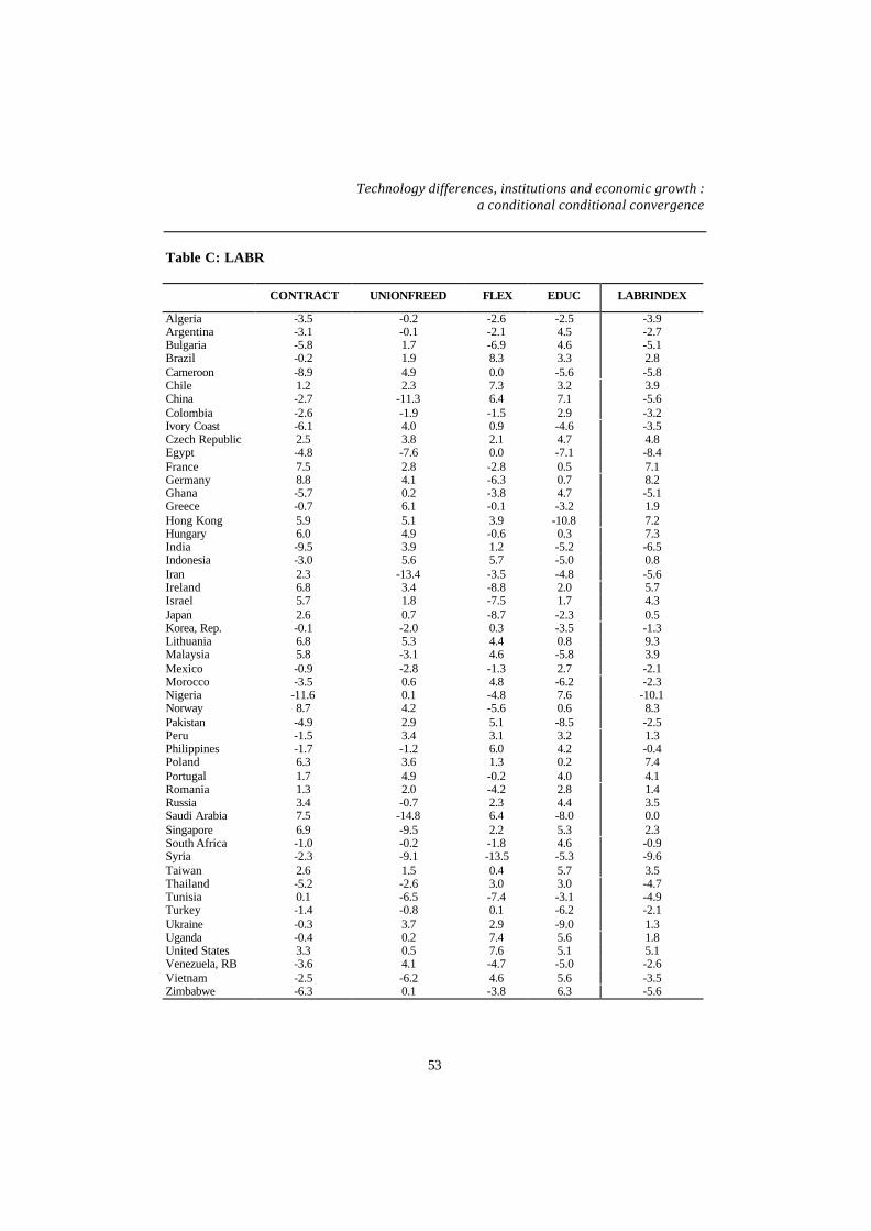
Technology differences, institutions and economic growth :a conditional conditional convergence
53
Table C: LABR
CONTRACT UNIONFREED FLEX EDUC LABRINDEX
Algeria -3.5 -0.2 -2.6 -2.5 -3.9Argentina -3.1 -0.1 -2.1 4.5 -2.7Bulgaria -5.8 1.7 -6.9 4.6 -5.1Brazil -0.2 1.9 8.3 3.3 2.8Cameroon -8.9 4.9 0.0 -5.6 -5.8Chile 1.2 2.3 7.3 3.2 3.9China -2.7 -11.3 6.4 7.1 -5.6Colombia -2.6 -1.9 -1.5 2.9 -3.2Ivory Coast -6.1 4.0 0.9 -4.6 -3.5Czech Republic 2.5 3.8 2.1 4.7 4.8Egypt -4.8 -7.6 0.0 -7.1 -8.4France 7.5 2.8 -2.8 0.5 7.1Germany 8.8 4.1 -6.3 0.7 8.2Ghana -5.7 0.2 -3.8 4.7 -5.1Greece -0.7 6.1 -0.1 -3.2 1.9Hong Kong 5.9 5.1 3.9 -10.8 7.2Hungary 6.0 4.9 -0.6 0.3 7.3India -9.5 3.9 1.2 -5.2 -6.5Indonesia -3.0 5.6 5.7 -5.0 0.8Iran 2.3 -13.4 -3.5 -4.8 -5.6Ireland 6.8 3.4 -8.8 2.0 5.7Israel 5.7 1.8 -7.5 1.7 4.3Japan 2.6 0.7 -8.7 -2.3 0.5Korea, Rep. -0.1 -2.0 0.3 -3.5 -1.3Lithuania 6.8 5.3 4.4 0.8 9.3Malaysia 5.8 -3.1 4.6 -5.8 3.9Mexico -0.9 -2.8 -1.3 2.7 -2.1Morocco -3.5 0.6 4.8 -6.2 -2.3Nigeria -11.6 0.1 -4.8 7.6 -10.1Norway 8.7 4.2 -5.6 0.6 8.3Pakistan -4.9 2.9 5.1 -8.5 -2.5Peru -1.5 3.4 3.1 3.2 1.3Philippines -1.7 -1.2 6.0 4.2 -0.4Poland 6.3 3.6 1.3 0.2 7.4Portugal 1.7 4.9 -0.2 4.0 4.1Romania 1.3 2.0 -4.2 2.8 1.4Russia 3.4 -0.7 2.3 4.4 3.5Saudi Arabia 7.5 -14.8 6.4 -8.0 0.0Singapore 6.9 -9.5 2.2 5.3 2.3South Africa -1.0 -0.2 -1.8 4.6 -0.9Syria -2.3 -9.1 -13.5 -5.3 -9.6Taiwan 2.6 1.5 0.4 5.7 3.5Thailand -5.2 -2.6 3.0 3.0 -4.7Tunisia 0.1 -6.5 -7.4 -3.1 -4.9Turkey -1.4 -0.8 0.1 -6.2 -2.1Ukraine -0.3 3.7 2.9 -9.0 1.3Uganda -0.4 0.2 7.4 5.6 1.8United States 3.3 0.5 7.6 5.1 5.1Venezuela, RB -3.6 4.1 -4.7 -5.0 -2.6Vietnam -2.5 -6.2 4.6 5.6 -3.5Zimbabwe -6.3 0.1 -3.8 6.3 -5.6

CEPII, Working Paper No 2004 - 02
54
Table A: FIN
Significance Tests Based on 51 Observations
Test DF Chi-Square Prob > ChiSq
H0 : No common factorsHA : At least one common factor
231 630.59 <.0001
H0 : 5 Factors are sufficientHA : More factors are needed
131 139.74 0.2846
Chi-Sqare without Bartlett’s Correction 181.48Akaike’s Information Criterion -80.52Schwarz’s Bayesian Criterion -333.59Tucker and Lewis’s Reliability Coeeficient 0.9614
Eigen ValuesContribution rotation NbFACTOR
Factor1 0.335 0.246 5Factor2 0.157 0.088 5Factor3 0.086 0.106 5Factor4 0.073 0.197 5Factor5 0.067 0.080 5
sum 0.717 0.717 .
Table B: FIN
Rotated Factors Important Variables Interpretation Variable Names CommentsFactor 1 C601 c703 c704
c705Bank control, rules (Cookratio, normalised account.
system), transparency
BANKRULES
Factor 2 C801 c701 c700c400
Domestic and internationalcompetition
COMPET
Factor 3 C901 c600 c900-c402
Credit access and non-independence of the central
bank
CREDIT
Factor 4 C602 State guaranty on deposits DEPGUARANFactor 5 C702 Promoting competition and
debtors protection?Fc702

Technology differences, institutions and economic growth :a conditional conditional convergence
55
Table C: FIN
BANKRULES COMPET CREDIT DEPGUARANT Fc702 FININDEXAlgeria -3.3 -6.7 3.8 4.0 1.5 -4.1Argentina 2.2 4.0 -4.0 3.4 -6.0 3.2Bulgaria 2.1 -1.5 -11.1 3.4 0.9 -0.2Brazil -3.9 -0.2 7.8 4.1 0.2 -0.5Cameroon -5.2 -0.3 2.8 -5.2 -5.7 -5.8Chile 4.8 3.2 2.0 2.7 -7.1 5.6China -5.2 -6.1 4.1 -4.9 4.5 -7.2Colombia -2.6 5.6 -1.1 5.4 -6.3 1.4Ivory Coast 2.2 6.7 6.6 -5.7 -7.7 4.0Czech Republic -4.7 1.3 6.7 5.0 2.0 0.0Egypt -5.9 -0.9 -6.1 3.7 -1.1 -5.3France 3.4 4.2 6.7 -5.3 7.9 5.7Germany 7.3 -1.5 1.8 4.4 7.6 7.4Ghana 1.7 0.1 -4.7 -5.4 -6.5 -1.9Greece 6.9 -4.1 7.2 3.8 7.3 6.5Hong Kong 8.6 2.4 -2.3 -7.7 -2.8 5.0Hungary 2.3 6.8 4.9 3.7 0.4 7.3India 0.5 0.0 -7.2 -6.4 6.8 -1.9Indonesia -5.7 9.6 0.1 -4.6 -0.9 -0.7Iran -7.2 -11.4 -3.8 -4.7 1.5 -13.4Ireland 9.7 -7.8 1.1 5.1 -8.4 3.9Israel 6.9 -10.9 3.8 3.3 -5.8 0.5Japan -1.6 4.3 0.1 2.9 9.5 3.0Korea, Rep. -1.4 4.9 -4.3 4.3 5.6 2.6Lithuania -3.8 -0.5 4.0 5.6 0.4 -0.8Malaysia 3.3 -0.6 -4.2 -5.6 -1.6 -0.3Mexico -3.5 7.1 1.9 4.1 -6.1 1.8Morocco -0.4 5.0 -7.2 -5.9 7.1 0.2Nigeria -5.2 7.4 -2.6 -5.9 -0.9 -2.3Norway 7.3 -2.4 0.7 3.8 7.1 6.4Pakistan -9.1 2.0 -1.5 4.8 -0.9 -5.0Peru -1.1 2.5 -4.1 5.4 -5.6 0.4Philippines 1.0 4.9 -0.1 4.0 -5.1 3.8Poland 2.3 7.6 7.6 -5.4 8.5 6.9Portugal 2.6 -2.8 -1.3 4.3 2.6 1.8Romania -4.9 -2.8 5.2 4.9 0.5 -2.9Russia -2.6 1.5 7.7 -5.3 -3.1 -1.6Saudi Arabia 2.4 -3.7 6.9 -6.0 1.4 -0.2Singapore 10.4 -5.8 -3.6 -6.7 -1.6 2.3South Africa 3.9 -1.3 2.0 -5.7 2.1 1.4Syria -10.4 -11.5 -0.8 -4.7 0.1 -15.5Taiwan -1.1 2.2 -9.3 4.5 7.1 0.6Thailand 1.5 1.0 -0.2 -6.5 -3.3 -0.6Tunisia -2.2 -2.9 -10.3 3.6 3.1 -3.8Turkey -3.2 0.5 3.9 6.2 -3.3 -0.2Ukraine 2.1 -4.2 2.8 5.2 -1.1 1.3Uganda -3.6 -1.5 3.1 -5.4 -1.9 -4.7United States 6.5 4.4 -2.9 2.9 6.5 8.4Venezuela, RB 1.0 -1.6 -5.8 4.7 -3.0 -0.3Vietnam -8.4 -6.5 -0.7 -4.9 1.9 -11.2Zimbabwe 3.2 0.2 -6.0 -5.6 -8.1 -1.1
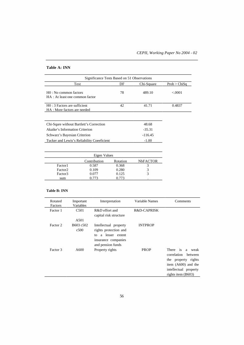
CEPII, Working Paper No 2004 - 02
56
Table A: INN
Significance Tests Based on 51 Observations
Test DF Chi-Square Prob > ChiSq
H0 : No common factorsHA : At least one common factor
78 489.10 <.0001
H0 : 3 Factors are sufficientHA : More factors are needed
42 41.71 0.4837
Chi-Sqare without Bartlett’s Correction 48.68Akaike’s Information Criterion -35.31Schwarz’s Bayesian Criterion -116.45Tucker and Lewis’s Reliability Coeeficient -1.00
Eigen Values
Contribution Rotation NbFACTORFactor1 0.587 0.368 3Factor2 0.109 0.280 3Factor3 0.077 0.125 3
sum 0.773 0.773 .
Table B: INN
RotatedFactors
ImportantVariables
Interpretation Variable Names Comments
Factor 1 C501
A501
R&D effort andcapital risk structure
R&D-CAPRISK
Factor 2 B603 c502c500
Intellectual propertyrights protection andto a lesser extentinsurance companiesand pension funds
INTPROP
Factor 3 A600 Property rights PROP There is a weakcorrelation betweenthe property rightsitem (A600) and theintellectual propertyrights item (B603)
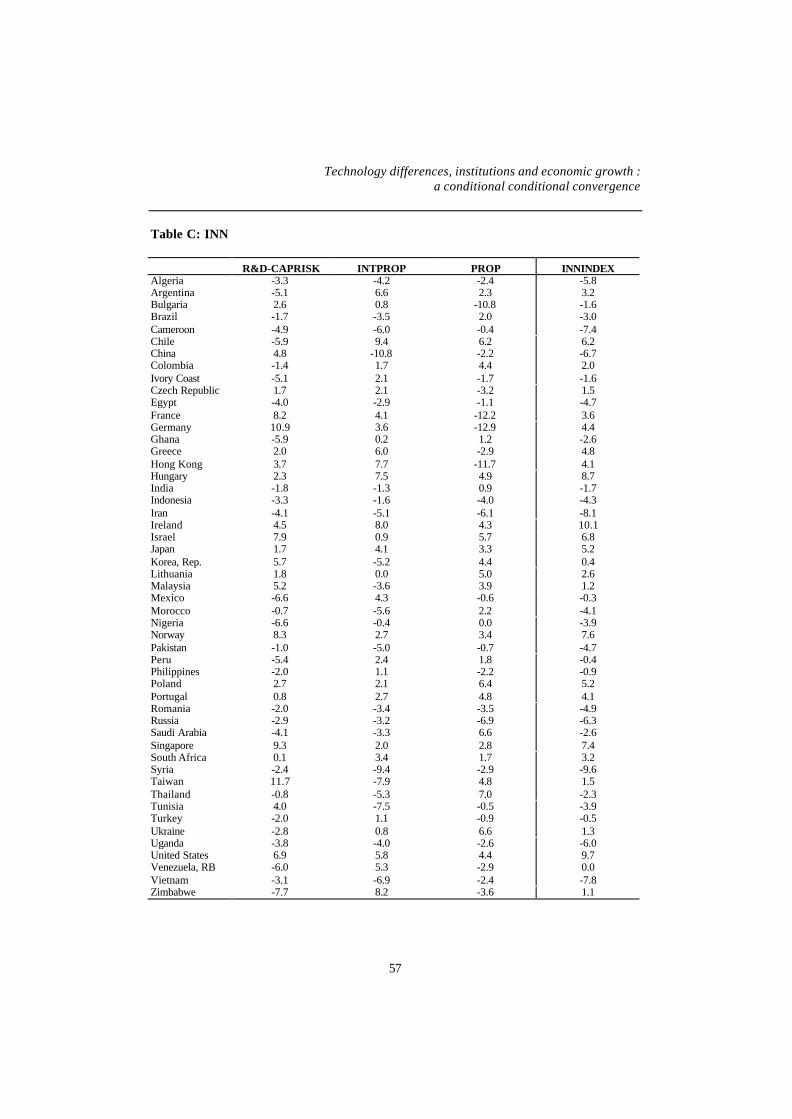
Technology differences, institutions and economic growth :a conditional conditional convergence
57
Table C: INN
R&D-CAPRISK INTPROP PROP INNINDEXAlgeria -3.3 -4.2 -2.4 -5.8Argentina -5.1 6.6 2.3 3.2Bulgaria 2.6 0.8 -10.8 -1.6Brazil -1.7 -3.5 2.0 -3.0Cameroon -4.9 -6.0 -0.4 -7.4Chile -5.9 9.4 6.2 6.2China 4.8 -10.8 -2.2 -6.7Colombia -1.4 1.7 4.4 2.0Ivory Coast -5.1 2.1 -1.7 -1.6Czech Republic 1.7 2.1 -3.2 1.5Egypt -4.0 -2.9 -1.1 -4.7France 8.2 4.1 -12.2 3.6Germany 10.9 3.6 -12.9 4.4Ghana -5.9 0.2 1.2 -2.6Greece 2.0 6.0 -2.9 4.8Hong Kong 3.7 7.7 -11.7 4.1Hungary 2.3 7.5 4.9 8.7India -1.8 -1.3 0.9 -1.7Indonesia -3.3 -1.6 -4.0 -4.3Iran -4.1 -5.1 -6.1 -8.1Ireland 4.5 8.0 4.3 10.1Israel 7.9 0.9 5.7 6.8Japan 1.7 4.1 3.3 5.2Korea, Rep. 5.7 -5.2 4.4 0.4Lithuania 1.8 0.0 5.0 2.6Malaysia 5.2 -3.6 3.9 1.2Mexico -6.6 4.3 -0.6 -0.3Morocco -0.7 -5.6 2.2 -4.1Nigeria -6.6 -0.4 0.0 -3.9Norway 8.3 2.7 3.4 7.6Pakistan -1.0 -5.0 -0.7 -4.7Peru -5.4 2.4 1.8 -0.4Philippines -2.0 1.1 -2.2 -0.9Poland 2.7 2.1 6.4 5.2Portugal 0.8 2.7 4.8 4.1Romania -2.0 -3.4 -3.5 -4.9Russia -2.9 -3.2 -6.9 -6.3Saudi Arabia -4.1 -3.3 6.6 -2.6Singapore 9.3 2.0 2.8 7.4South Africa 0.1 3.4 1.7 3.2Syria -2.4 -9.4 -2.9 -9.6Taiwan 11.7 -7.9 4.8 1.5Thailand -0.8 -5.3 7.0 -2.3Tunisia 4.0 -7.5 -0.5 -3.9Turkey -2.0 1.1 -0.9 -0.5Ukraine -2.8 0.8 6.6 1.3Uganda -3.8 -4.0 -2.6 -6.0United States 6.9 5.8 4.4 9.7Venezuela, RB -6.0 5.3 -2.9 0.0Vietnam -3.1 -6.9 -2.4 -7.8Zimbabwe -7.7 8.2 -3.6 1.1

CEPII, Working Paper No 2004 - 02
58
LIST OF WORKING PAPERS RELEASED BY CEPII14
No Title Authors
2004-01 Croissance et régimes d’investissement P. Villa
2003-22 A New Look at the Feldstein-Horioka Puzzle using anIntegrated Panel
A.BanerjeeP. Zanghieri
2003-21 Trade Linkages and Exchange Rates in Asia : TheRole of China
A. Bénassy-Quéré &Aminal Lahrèche-Révil
2003-20 Economic Implications of Trade Liberalization Underthe Doha Round
J. Francois,H. Van Meijl,
F. Van Tongeren2003-19 Methodological Tools for SIA – Report of the CEPII
Worshop held on 7-8 November 2002 in BrusselsN. Kousnetzoff
2003-18 Order Flows, Delta Hedging and Exchange RateDynamics
B. Rzepkowski
2003-17 Tax competition and Foreign Direct Investment A. Bénassy-Quéré,L. Fontagné & A.
Lahrèche-Révil
2003-16 Commerce et transfert de technologies : les cascomparés de la Turquie, de l’Inde et de la Chine
F. Lemoine &D. Ünal-Kesenci
2003-15 The Empirics of Agglomeration and Trade K. Head & T. Mayer
2003-14 Notional Defined Contribution: A Comparison of theFrench and German Point Systems
F. Legros
2003-13 How Different is Eastern Europe? Structure andDeterminants of Location Choices by French Firms inEastern and Western Europe
C. Disdier &T. Mayer
2003-12 Market Access Liberalisation in the Doha Round:Scenarios and Assessment
L. Fontagné, J.L.Guérin & S. Jean
2003-11 On the Adequacy of Monetary Arrangements in Sub-Saharian Africa
A. Bénassy-Quéré &Maylis Coupet
14
Working papers are circulated free of charge as far as stocks are available; thank you to send your requestto CEPII, Sylvie Hurion, 9, rue Georges-Pitard, 75015 Paris, or by fax : (33) 01 53 68 55 04 or by [email protected]. Also available on: \\www.cepii.fr. Working papers with * are out of print. They cannevertheless be consulted and downloaded from this website.14
Les documents de travail sont diffusés gratuitement sur demande dans la mesure des stocks disponibles.Merci d’adresser votre demande au CEPII, Sylvie Hurion, 9, rue Georges-Pitard, 75015 Paris, ou parfax : (33) 01 53 68 55 04 ou par e-mail [email protected]. Egalement disponibles sur : \\www.cepii.fr.Les documents de travail comportant * sont épuisés. Ils sont toutefois consultable sur le web CEPII.

Technology differences, institutions and economic growth :a conditional conditional convergence
59
2003-10 The Impact of EU Enlargement on Member States : aCGE Approach
H. Bchir, L. Fontagné& P. Zanghieri
2003-09 India and the World Economy : TraditionalSpecialisations and Technology Niches
S. Chauvin &F. Lemoine
2003-08 Imination Amongst Exchange-Rate Forecasters :Evidence from Survey Data
M. Beine,A. Bénassy-Quéré &
H. Colas
2003-07 Le Currency Board à travers l’expérience del’Argentine
S. Chauvin & P. Villa
2003-06 Trade and Convergence : Revisiting Ben-David G. Gaulier
2003-05 Estimating the Fundamental Equilibrium Exchange-Rate of Central and Eastern European Countries theEMU Enlargement Perspective
B Egert &A. Lahrèche-Revil
2003-04 Skills, Technology and Growth is ICT the Key toSuccess
J. Melka, L. Nayman,S. Signano &
N. Mulder
2003-03 L’investissement en TIC aux Etats-Unis et dansquelques pays européens
G. Cette & P.A. Noual
2003-02 Can Business and Social Networks Explain the BorderEffect Puzzle?
P.P. Combes,M. Lafourcade &
T. Mayer2003-01 Hyperinflation and the Reconstruction of a National
Money: Argentina and Brazil, 1990-2002J. Sgard
2002-18 Programme de travail du CEPII pour 2003
2002-17 MIRAGE, a Computable General Equilibrium Modelfor Trade Policy Analysis
M.H. Bchir,Y. Decreux,
J.L. Guérin & S. Jean2002-16 Evolutions démographiques et marché du travail : des
liens complexes et parfois contradictoiresL. Cadiou, J. Genet &
J.L. Guérin
2002-15 Exchange Rate Regimes and Sustainable Parities forCEECs in the Run-up to EMU Membership
V. Coudert &C. Couharde
2002-14 When are Structural Deficits Good Policies? J. Chateau
2002-13 Projections démographiques de quelques pays del’Union Européenne (Allemagne, France, Italie,Royaume-Uni, Pays-Bas, Suède)
R. Sleiman
2002-12 Regional Trade Integration in Southern Africa S. Chauvin &G. Gaulier
2002-11 Demographic Evolutions and Unemployment: anAnalysis of French Labour Market with Workers
J. Château, J.L. Guérin& F. Legros

CEPII, Working Paper No 2004 - 02
60
Generations
2002-10 Liquidité et passage de la valeur P. Villa
2002-09 Le concept de coût d’usage Putty-Clay des biensdurables
M.G. Foggea &P. Villa
2002-08 Mondialisation et régionalisation : le cas des industriesdu textile et de l’habillement
M. Fouquin, P. MorandR. Avisse G. Minvielle
& P. Dumont2002-07 The Survival of Intermediate Exchange Rate Regimes A. Bénassy-Quéré &
B. Coeuré2002-06 Pensions and Savings in a Monetary Union : An
Analysis of Capital FlowA. Jousten & F. Legros
2002-05 Brazil and Mexico’s Manufacturing Performance inInternational Perspective, 1970-1999
N. Mulder, S. Montout& L. Peres Lopes
2002-04 The Impact of Central Bank Intervention onExchange-Rate Forecast Heterogeneity
M. Beine,A. Benassy-Quéré,
E. Dauchy &R. MacDonald
2002-04 The Impact of Central Bank Intervention on ForecastHeterogeneity
M. Beine,A. Benassy-Quéré,
E. Dauchi &R. MacDonald
2002-03 Impacts économiques et sociaux de l’élargissementpour l’Union européenne et la France
M.H. Bchir &M. Maurel
2002-02 China in the International Segmentation of ProductionProcesses
F. Lemoine &D. Ünal-Kesenci
2002-01 Illusory Border Effects: Distance MismeasurementInflates Estimates of Home Bias in Trade
K Head & T. Mayer
2001-22 Programme de travail du CEPII pour 2002
2001-21 Croissance économique mondiale : un scénario deréférence à l’horizon 2030
N. Kousnetzoff
2001-20 The Fiscal Stabilization Policy under EMU – AnEmpirical Assessment
A. Kadareja
2001-19 Direct Foreign Investments and Productivity Growthin Hungarian Firms, 1992-1999
J. Sgard
2001-18 Market Access Maps: A Bilateral and DisaggregatedMeasure of Market Access
A. Bouët, L. Fontagné,M. Mimouni &
X. Pichot
2001-17 Macroeconomic Consequences of Pension Reforms inEurope: An Investigation with the INGENUE World
Equipe Ingénue

Technology differences, institutions and economic growth :a conditional conditional convergence
61
Model
2001-16* La productivité des industries méditerranéennes A. Chevallier &D. Ünal-Kesenci
2001-15 Marmotte: A Multinational Model L. Cadiou, S. Dees,S. Guichard,A. Kadareja,
J.P. Laffargue &B. Rzepkowski
2001-14 The French-German Productivity ComparisonRevisited: Ten Years After the German Unification
L. Nayman &D. Ünal-Kesenci
2001-13* The Nature of Specialization Matters for Growth: AnEmpirical Investigation
I. Bensidoun,G. Gaulier
& D. Ünal-Kesenci
2001-12 Forum Economique Franco-Allemand - Deutsch-Französisches Wirtschaftspolitisches Forum, PoliticalEconomy of the Nice Treaty: Rebalancing the EUCouncil and the Future of European AgriculturalPolicies, 9th meeting, Paris, June 26th 2001
2001-11 Sector Sensitivity to Exchange Rate Fluctuations M. Fouquin, K. Sekkat,J. Malek Mansour,
N. Mulder &L. Nayman
2001-10* A First Assessment of Environment-Related TradeBarriers
L. Fontagné, F. vonKirchbach &M. Mimouni
2001-09 International Trade and Rend Sharing in Developedand Developing Countries
L. Fontagné &D. Mirza
2001-08 Economie de la transition : le dossier G. Wild
2001-07 Exit Options for Argentina with a Special Focus onTheir Impact on External Trade
S. Chauvin
2001-06 Effet frontière, intégration économique et 'ForteresseEurope'
T. Mayer
2001-05 Forum Économique Franco-Allemand – Deutsch-Französisches Wirtschaftspolitisches Forum, TheImpact of Eastern Enlargement on EU-LabourMarkets and Pensions Reforms between Economicand Political Problems, 8th meeting, Paris, January 162001

CEPII, Working Paper No 2004 - 02
62
2001-04 Discrimination commerciale : une mesure à partir desflux bilatéraux
G. Gaulier
2001-03* Heterogeneous Expectations, Currency Options andthe Euro/Dollar Exchange Rate
B. Rzepkowski
2001-02 Defining Consumption Behavior in a Multi-CountryModel
O. Allais, L. Cadiou &S. Dées
2001-01 Pouvoir prédictif de la volatilité implicite dans le prixdes options de change
B. Rzepkowski
2000-22 Forum Economique Franco-Allemand - Deutsch-Französisches Wirtschaftspolitisches Forum, TradeRules and Global Governance: A long Term Agendaand The Future of Banking in Europe, 7th meeting,Paris, July 3-4 2000
2000-21 The Wage Curve: the Lessons of an Estimation Over aPanel of Countries
S. Guichard &J.P. Laffargue
2000-20 A Computational General Equilibrium Model withVintage Capital
L. Cadiou, S. Dées &J.P. Laffargue
2000-19 Consumption Habit and Equity Premium in the G7Countries
O. Allais, L. Cadiou &S. Dées
2000-18 Capital Stock and Productivity in French Transport:An International Comparison
B. Chane Kune &N. Mulder
2000-17 Programme de travail 2001
2000-16 La gestion des crises de liquidité internationale :logique de faillite, prêteur en dernier ressort etconditionnalité
J. Sgard
2000-15 La mesure des protections commerciales nationales A. Bouët
2000-14 The Convergence of Automobile Prices in theEuropean Union: An Empirical Analysis for thePeriod 1993-1999
G. Gaulier & S. Haller
2000-13* International Trade and Firms’ Heterogeneity UnderMonopolistic Competition
S. Jean
2000-12 Syndrome, miracle, modèle polder et autresspécificités néerlandaises : quels enseignements pourl’emploi en France ?
S. Jean
2000-11 FDI and the Opening Up of China’s Economy F. Lemoine
2000-10 Big and Small Currencies: The Regional Connection A. Bénassy-Quéré &B. Coeuré

Technology differences, institutions and economic growth :a conditional conditional convergence
63
2000-09* Structural Changes in Asia And Growth ProspectsAfter the Crisis
J.C. Berthélemy &S. Chauvin
2000-08 The International Monetary Fund and the InternationalFinancial Architecture
M. Aglietta
2000-07 The Effect of International Trade on Labour-DemandElasticities: Intersectoral Matters
S. Jean
2000-06 Foreign Direct Investment and the Prospects for TaxCo-Ordination in Europe
A. Bénéssy-Quéré,L. Fontagné &
A. Lahrèche-Révil
2000-05 Forum Economique Franco-Allemand - Deutsch-Französisches Wirtschaftspolitisches Forum,Economic Growth in Europe Entering a NewArea?/The First Year of EMU, 6th meeting, Bonn,January 17-18, 2000
2000-04* The Expectations of Hong Kong Dollar Devaluationand their Determinants
B. Rzepkowski
2000-03 What Drove Relative Wages in France? StructuralDecomposition Analysis in a GeneralEquilibrium Framework, 1970-1992
S. Jean & O. Bontout
2000-02 Le passage des retraites de la répartition à lacapitalisation obligatoire : des simulations à l’aided’une maquette
O. Rouguet & P. Villa
2000-01* Rapport d’activité 1999
1999-16 Exchange Rate Strategies in the Competition forAttracting FDI
A. Bénassy-Quéré,L. Fontagné &
A. Lahrèche-Révil
1999-15 Groupe d’échanges et de réflexion sur la Caspienne.Recueil des comptes-rendus de réunion (déc. 97- oct.98)"
D. Pianelli &G. Sokoloff
1999-14 The Impact of Foreign Exchange Interventions: NewEvidence from FIGARCH Estimations
M. Beine,A. Bénassy-Quéré &
C. Lecourt
1999-13 Forum Economique Franco-Allemand - Deutsch-Französisches Wirtschaftspolitisches Forum,Reduction of Working Time/Eastward Enlargment ofthe European Union, 5 th meeting, Paris, July 6-7 1999
1999-12* A Lender of Last Resort for Europe M. Aglietta
1999-11* La diversité des marchés du travail en Europe :Quelles conséquences pour l’Union Monétaire ;
L. Cadiou, S. Guichard

CEPII, Working Paper No 2004 - 02
64
Deuxième partie : Les implications macro-économiques de la diversité des marchés du travail
& M. Maurel
1999-10* La diversité des marchés du travail en Europe :Quelles conséquences pour l’Union Monétaire ;Première partie : La diversité des marchés du travaildans les pays de l’Union Européenne
L. Cadiou &S. Guichard
1999-09 The Role of External Variables in the ChineseEconomy; Simulations from a macroeconometricmodel of China
S. Dees
1999-08 Haute technologie et échelles de qualité : de fortesasymétries en Europe
L. Fontagné,M. Freudenberg &
D. Ünal-Kesenci
1999-07 The Role of Capital Accumultion, Adjustment andStructural Change for Economic Take-Off: EmpiricalEvidence from African Growth Episodes
J.C. Berthélemy &L. Söderling
1999-06 Enterprise Adjustment and the Role of Bank Credit inRussia: Evidence from a 420 Firm’s QualitativeSurvey
S. Brana, M. Maurel &J. Sgard
1999-05 Central and Eastern European Countries in theInternational Division of Labour in Europe
M. Freudenberg &F. Lemoine
1999-04 Forum Economique Franco-Allemand – EconomicPolicy Coordination – 4 th meeting, Bonn, January 11-12 1999
1999-03 Models of Exchange Rate Expectations:Heterogeneous Evidence From Panel Data
A. Bénassy-Quéré,S. Larribeau &R. MacDonald
1999-02 Forum Economique Franco-Allemand – LabourMarket & Tax Policy in the EMU
1999-01 Programme de travail 1999

CEPII, Working Paper No 2003 - ? ?
CEPIIDOCUMENTS DE TRAVAIL / WORKING PAPERS
Si vous souhaitez recevoir des Documents de travail,merci de remplir le coupon-réponse ci-joint et de le retourner à :
Should you wish to receive copies of the CEPII’s Working papers,just fill the reply card and return it to:
Sylvie HURION – PublicationsCEPII – 9, rue Georges-Pitard – 75740 Paris – Fax : (33) 1.53.68.55.04
M./Mme / Mr./Mrs ................................................................................................................................
Nom-Prénom / Name-First name .........................................................................................................
Titre / Title ...............................................................................................................................................
Service / Department..............................................................................................................................
Organisme / Organisation .....................................................................................................................
Adresse / Address...................................................................................................................................
Ville & CP / City & post code .............................................................................................................Pays / Country...................................................................... Tél. ...........................................................
Désire recevoir les Document de travail du CEPII n° :
Wish to receive the CEPII’s Working Papers No: ..........................................................................
...................................................................................................................................................................
...................................................................................................................................................................
...................................................................................................................................................................
...................................................................................................................................................................
...................................................................................................................................................................
...................................................................................................................................................................
...................................................................................................................................................................
c Souhaite être placé sur la liste de diffusion permanente (pour les bibliothèques)Wish to be placed on the standing mailing list (for Libraries).