Technology and the Theory of Vintage Aggregation - National

This PDF is a selection from a published volume from theNational Bureau of Economic Research

Volume Title: Hard-to-Measure Goods and Services: Essaysin Honor of Zvi Griliches

Volume Author/Editor: Ernst R. Berndt and Charles R. Hulten,editors

Volume Publisher: University of Chicago Press

Volume ISBN: 0-226-04449-1; 978-0-226-04449-1

Volume URL: http://www.nber.org/books/bern07-1

Conference Date: September 19-20, 2003

Publication Date: October 2007

Title: Technology and the Theory of Vintage Aggregation

Author: Michael J. Harper

URL: http://www.nber.org/chapters/c0875

99

4.1 Introduction

When vintage investments are aggregated into “capital stocks,” rigid as-sumptions are made about the effects of technology. This can limit the use-fulness of capital stock measures. Vintage aggregation issues were the sub-ject of a vigorous literature in the 1950s and 1960s, and Zvi Griliches (1963)was an active participant in these discussions. By the 1970s, many econo-mists considered these issues to be resolved, and they have received less at-tention in recent decades. The acceleration of information processing andcommunications technologies in the 1990s, however, may increase the po-tential for bias in capital stock measures. This accelerating technologicalprogress has had many ramifications for economic measurement in theUnited States. Our National Income and Product Accounts did not ac-count for the quality change in computers until Jack Triplett (1989) pro-posed adjusting Computer Price Indexes for quality change with hedonicmethods. As Charles Hulten (1992) observed, the Triplett treatment iden-tifies quality change with embodied technical change, as Robert Hall(1968) had defined it. Once these hedonic methods were in place, growth

4Technology and the Theory of Vintage Aggregation

Michael J. Harper

I only want to urge that research not get tied to any one partic-ular picture of the way the economy functions.—Robert Solow (2001)

Michael J. Harper is Associate Commissioner for Productivity and Technology at the Bu-reau of Labor Statistics.

The views expressed are those of the author and do not necessarily reflect the policies of theU.S. Bureau of Labor Statistics or the views of other staff members. An early draft of this pa-per was presented at the NBER Summer Institute in 1999, where Zvi Griliches made helpfulcomments. I would also like to acknowledge Anthony Barkume, Ernst Berndt, Carol Cor-rado, Edwin Dean, W. Erwin Diewert, Murray Foss, Robert Gordon, Charles Hulten, Mari-lyn Manser, Peter Meyer, Linda Moeller, Phyllis Otto, Sabrina Pabilonia, Matthew Shapiro,Daniel Sichel, Brian Sliker, Leo Sveikauskas, Jack Triplett, and Cynthia Zoghi for helpfulcomments, suggestions, and encouragement at various stages of this line of work. Any errorsare entirely my own.

accounting studies by Stephen Oliner and Daniel Sichel (2000) and by DaleJorgenson and Kevin Stiroh (2001) concluded that computer quality was,perhaps, the most important source of U.S. productivity growth in the late1990s. However, European national accountants found reasons to be skep-tical. For example, Peter Hill (2000) pointed out that quality adjustmentsmade from vintage accounts of prices reflected only the positive aspects ofquality change while neglecting some negative effects.

This paper uses diagrams as well as formal definitions to shed some lighton the implications of the rigid assumptions about vintage aggregationmade in our standard total factor productivity work. The approach ap-peals to two different models of how technology and capital formation canexplain growth in labor productivity, both proposed by Robert Solow(1957, 1960). The first model assumed that technology was “disembodied”in that it raised productivity independently of the level of investment. Vin-tage investments were summarized in a “capital stock” measure that wasused to separate the contributions of capital and of “residual” technologychange to labor productivity growth. This first model is the basis for mod-ern neoclassical total factor productivity exercises. In the second Solowmodel, technology was “embodied” in capital, and the contribution ofeach “vintage” of capital to labor productivity could be different. This sec-ond model was equally rooted in neoclassical concepts, but it did not makethe rigid assumptions needed to build a capital stock. Instead, Solow de-scribed the dynamic allocation of labor among capital of different vintages.

After a brief review of relevant material on models of production, capi-tal measurement, and quality adjustment (section 4.2), this paper developsa “model of production with machines” (section 4.3) in which the Solowvintage model is extended to individual machines. This machine modelpermits clearer definitions of key concepts such as deterioration and em-bodied and disembodied technical change. The machine model predicts thatolder vintages are preferentially discarded during a cyclical downturn.This realistic behavior is inconsistent with what is assumed in capital stockcalculations. Section 4.4 examines the machine model in nominal terms.

Section 4.5 considers the idea of real capital input. The machine model isused to clarify previous discussions of what the marginal product of capitalis—the added output obtained from a collection of machines by adding onemachine (not a machine hour) and without adding any labor. Section 4.6 dis-cusses how quality adjustments to capital inputs could be overstated.

4.2 Some Background on Models of Growth, Capital Stocks, and Quality Change

4.2.1 The Solow Residual Model

Solow’s (1957) residual model constructed an aggregate capital stock,K, and used it in a production function, f, of the form Y � f (L, K, t), where

100 Michael J. Harper

Y is a real value added output measure, L is labor hours, K is aggregate cap-ital stock, and t is the time of observation, to parse out the contributionsto labor productivity growth of capital and of shifts in the production func-tion.1 Solow showed that

(1) (y � l ) � sK(k � l ) � a,

where y, l, and k represent the growth rates of output, labor, and capitalstock, respectively, and where sK is the share of capital or property income,�, in the value of output. Property income is calculated using output prices,p, and wages, w, as the residual of labor compensation in nominal valueadded output: � � pY – wL. The “Solow residual,” a, is a measure of dis-embodied technical change in that it is presumed to contribute indepen-dently of the level of investment in capital. The growth rate of a is typicallydetermined as the residual of output growth not accounted for by growth incapital and labor inputs. Hulten (2001) reviewed many studies which havemeasured the residual, most commonly known as total factor productivitygrowth. The Bureau of Labor Statistics (BLS; 2001) produces measures ofa, which it calls multifactor productivity, using the same general methods.

Time series estimates of labor productivity and of a are procyclical. Thishas been a troubling problem for neoclassical models because a is designedto measure technological progress that should not be highly sensitive to thecycle. This issue was explored by Catherine Morrison and Ernst Berndt(1981). Many ideas, such as labor hoarding and disequilibrium, have beenput forth in an effort to reconcile apparent short-run increasing marginalreturns to labor with the neoclassical prediction of diminishing returns.Section 4.5 will show how the cyclical nature of the residual is partly a con-sequence of the rigidity with which capital is measured.

4.2.2 The Solow Vintage Model

“The controversies still rage[d]” when Harcourt (1969, 369) wrote his ac-count of a bitter debate in the literature over whether capital measurementis useful. An understanding of the issues had gradually emerged in the con-text of Leontief’s (1947) aggregation theorem. To build a stock, capital hadto be like jelly—the ratios of marginal products of different investmentscould not vary as functions of output or other inputs in the productionfunction. Empirically, the Leontief conditions are rarely satisfied. For ex-ample, newer electric power plants are used continuously while olderplants are reserved to meet peak demand. Another example is that one fastcomputer is not a perfect substitute for two slow machines for which the to-tal cost is the same because the latter are designed in most cases to workwith two people.

Technology and the Theory of Vintage Aggregation 101

1. The derivation involves differentiating the production function with respect to time, as-suming constant returns to scale, that input prices are given, and that inputs are paid the val-ues of their marginal products.

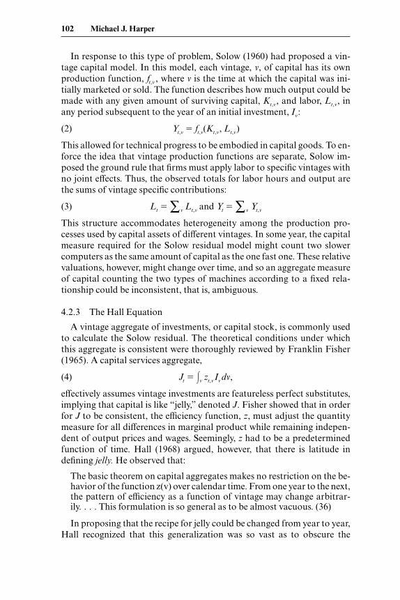
In response to this type of problem, Solow (1960) had proposed a vin-tage capital model. In this model, each vintage, v, of capital has its ownproduction function, ft,v , where v is the time at which the capital was ini-tially marketed or sold. The function describes how much output could bemade with any given amount of surviving capital, Kt,v, and labor, Lt,v, inany period subsequent to the year of an initial investment, Iv:

(2) Yt,v � ft,v(Kt,v, Lt,v)

This allowed for technical progress to be embodied in capital goods. To en-force the idea that vintage production functions are separate, Solow im-posed the ground rule that firms must apply labor to specific vintages withno joint effects. Thus, the observed totals for labor hours and output arethe sums of vintage specific contributions:

(3) Lt � ∑v Lt,v and Yt � ∑v Yt,v

This structure accommodates heterogeneity among the production pro-cesses used by capital assets of different vintages. In some year, the capitalmeasure required for the Solow residual model might count two slowercomputers as the same amount of capital as the one fast one. These relativevaluations, however, might change over time, and so an aggregate measureof capital counting the two types of machines according to a fixed rela-tionship could be inconsistent, that is, ambiguous.

4.2.3 The Hall Equation

A vintage aggregate of investments, or capital stock, is commonly usedto calculate the Solow residual. The theoretical conditions under whichthis aggregate is consistent were thoroughly reviewed by Franklin Fisher(1965). A capital services aggregate,

(4) Jt � �v zt,v Ivdv,

effectively assumes vintage investments are featureless perfect substitutes,implying that capital is like “jelly,” denoted J. Fisher showed that in orderfor J to be consistent, the efficiency function, z, must adjust the quantitymeasure for all differences in marginal product while remaining indepen-dent of output prices and wages. Seemingly, z had to be a predeterminedfunction of time. Hall (1968) argued, however, that there is latitude indefining jelly. He observed that:

The basic theorem on capital aggregates makes no restriction on the be-havior of the function z(v) over calendar time. From one year to the next,the pattern of efficiency as a function of vintage may change arbitrar-ily. . . . This formulation is so general as to be almost vacuous. (36)

In proposing that the recipe for jelly could be changed from year to year,Hall recognized that this generalization was so vast as to obscure the


capital-related phenomena addressed in previous literature. To reach aninterpretation, he proposed a structural form for z involving a decomposi-tion into three factors that he could loosely associate with important phe-nomena: functions of time (dt, disembodied technical change), of age (�t–v ,deterioration), and of vintage (bv , embodied technical change):

(5) Jt � �v zt,v Ivdv � dt �v �t�vbvIvdv

Hall then pointed out that functions dt, �t–v, and bv reflect only two inde-pendent influences, time and vintage, and so the specification can be writ-ten in terms of two functions, eliminating the third by including its influ-ence in respecified versions of the other two. This pulled the two Solowmodels together under a particular specification, which I will refer to asHall’s equation (5).

4.2.4 Quality Adjustment to Capital Measures

New improved models of high-tech equipment that embody improve-ments are frequently introduced and marketed alongside older models.Quality adjustment involves comparing prices of new improved goods tonew unimproved goods. I will define each asset’s model year, m, to be theyear in which assets with a given design were first sold. Capital goods priceswill be denoted using three subscripts, pK

t,v,m. In principle, a quality adjust-ment factor, b, can be defined by comparing the prices of brand new goods(v � t) of the latest model (m � t) to the prices of brand new goods of a pre-vious period’s model (m � t – 1). For example, matched models assume bm /bm–1 � p K

t,t,t /pKt,t,t–1. Hedonic models estimate b from wider sets of prices and

characteristics. Statistical agencies then measure real capital by deflatingmeasures of nominal capital expenditures, Et , with a price index thattracks the price for a new good of constant quality:

(6) �

This is equivalent to deflating with a quality-adjusted price index, that is,Jt /Jt–1 � (Et bt /p

Kt,t,t )/(Et bt–1/p

Kt–1,t–1,t–1). The quality-adjustment parameter

factor, b, would seem to be the right factor to use in Hall’s equation. How-ever, this presumes relative prices of capital goods reflect their relative mar-ginal products, a notion that will be critiqued in section 4.5.

4.3 A Model of Production with Machines

In this section, a model is developed describing production from indi-vidual machines, which could be almost any type of asset such as comput-ers, trucks, or buildings. As in section 4.2, three subscripts are used to de-note time, vintage, and model, where the model variable will be regarded asthe time at which machines with specific physical characteristics were first

(Et /pKt,t,t�1)

��(Et /p

Kt�1,t�1,t�1)

Jt�Jt�1


sold in the market. This third subscript will be used in the formulation ofdefinitions as well as in the description of available data on capital goodsprices. Solow’s vintage model (equation [2]) is modified to describe outputas a function of labor associated with specific models, m, as well as specificvintages, that is, Yt,v,m � ft,v,m(Kt,v,m, Lt,v,m ). At any time the economywidestocks of each vintage and model, Kt,v,m, will be regarded as fixed by pastinvestment decisions. A firm owning (and planning to keep) a machine, oftype t, v, m, faces the following short-run production possibilities for gen-erating output from labor:

(7) � gt,v,m� �The capital variable, Kt,v,m, involves aggregation across machines of type

t, v, m. I will treat these machines as identical, but I will consider their dis-crete nature rather than treating Kt,v,m as jelly. Let Kt,v,m refer to the set of allmachines in existence at any time, t. Consider Kt,v,m to consist of discretenumbers, nt,v,m of identical machines. Assume that all machines in each vin-tage-model category are used identically at each point in time. Then totaloutput from all machines of each vintage-model combination will be nt,v,m

times the output of each machine. The machine production function, f, isthen defined in terms of output per machine, by vintage and model:

(8) � � � ft,v,m� � ∀ v, m ⊂ Kt,v,m

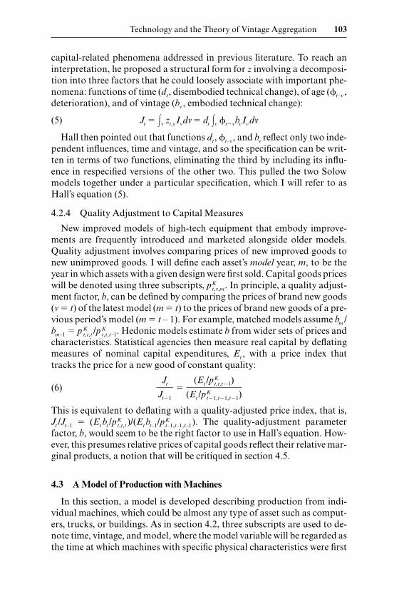
Assume that the output coming from each machine is a smooth function,f, of labor and is characterized by diminishing marginal returns to labor.Figure 4.1 depicts such a machine production function, f. If the firmchooses to operate at point A, the average product of labor (labor produc-tivity) will be the slope of ray OA and the marginal product of labor will bethe slope of the tangent to f at A.

I next extend Solow’s ground rule (equation [3]) so that labor is allocatedto specific machines to produce output:

(9) Lt � �v �m Lt,v,m dm dv and Yt � �v �m Yt,v,m dm dv

As in Solow’s vintage model, assume that output and labor can be mea-sured and that they are homogeneous. Also, cost minimization implies thatthe marginal product of labor applied to each machine will be the same(and will equal the wage rate relative to the price of output):

(10) � ∀ t, v, m

In figure 4.2, three machine functions are depicted. Expression (10) impliesthey will be operated at points where tangents are parallel. It is also im-portant to note that labor productivity differs by vintage (even though the

wt�pt

∂ft,v,m�∂Lt,v,m

Lt,v,m�nt,v,m

Yt,v,m�nt,v,m

Lt,v,m�Kt,v,m

Yt,v,m�Kt,v,m


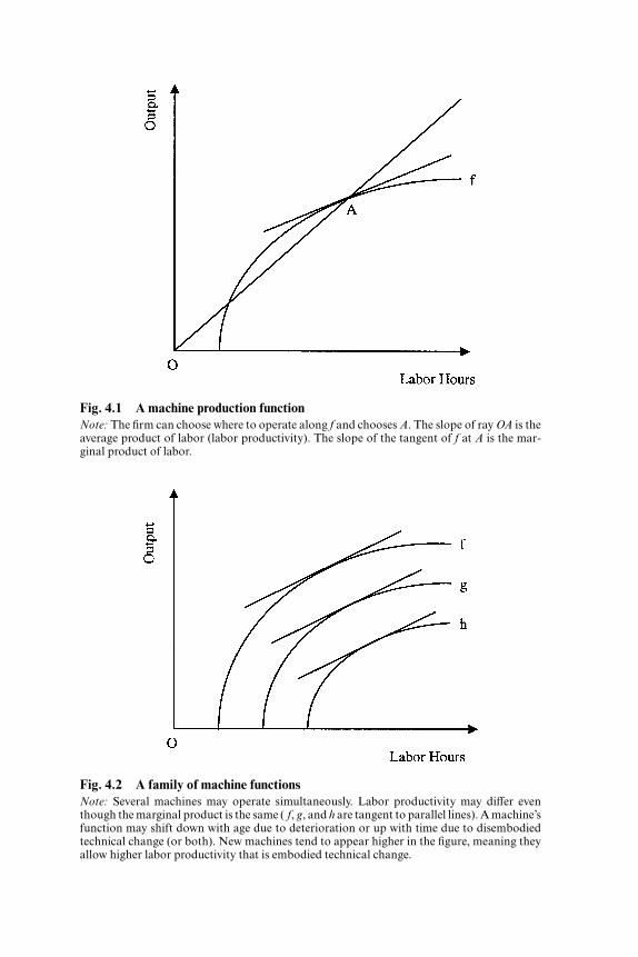
Fig. 4.1 A machine production functionNote: The firm can choose where to operate along f and chooses A. The slope of ray OA is theaverage product of labor (labor productivity). The slope of the tangent of f at A is the mar-ginal product of labor.

Fig. 4.2 A family of machine functionsNote: Several machines may operate simultaneously. Labor productivity may differ eventhough the marginal product is the same ( f, g, and h are tangent to parallel lines). A machine’sfunction may shift down with age due to deterioration or up with time due to disembodiedtechnical change (or both). New machines tend to appear higher in the figure, meaning theyallow higher labor productivity that is embodied technical change.

marginal product of labor is the same). In this situation, if wt /pt changed,labor would be reallocated in such a way that the marginal product of la-bor on all vintages would adjust proportionally to wt /pt , but note that theaverage product of labor could adjust differently on each vintage.

If this model were ever to be elaborated as thoroughly as Solow’s residualmodel, issues such as the heterogeneity of labor and of output (compositionor quality effects) and the relationships among different types of capitalmight be addressed. However, in order to facilitate exposition, this paperwill describe a situation where one type of output is made with one type oflabor using progressively advancing versions of one type of machine.

4.3.1 Relationships among Functions

Zvi Griliches (1963) made one of the most thorough efforts in the litera-ture to define the key concepts of capital measurement, such as replace-ment, depreciation, deterioration, obsolescence, and capital services. Thispaper will provide similar definitions that refer to the machine model. Inorder to facilitate compact mathematical definitions and analysis of phe-nomena associated with capital, it is assumed that machine productionfunctions, ft,v,m and related variables are continuous functions of time, vin-tage, and model.

As machines age, their physical characteristics change due to wear andtear. The rate of deterioration of output, � f

t,v,m, (the output decay rate) is de-fined as the rate at which the output produced by a given amount of laborwith a given model varies by vintage:

(11) � ft,v,m � �

As indicated, this will be the negative of the rate at which output varies byage alone for a given model. Note that the deterioration rate can vary withtime, vintage, or model. Newer models embody features that permit themto make more output with the same amount of labor. The rate at whichfunctions differ due to embodied technical change, B f

t,v,m, is defined in termsof models, or equivalently, model age:

(12) B ft,v,m � �

These are the only two types of shifts considered that are due solely to themachine’s physical characteristics. However, as time passes, people maylearn how to get more out of a given machine. Disembodied technicalchange, D f

t,v,m , is the rate at which the function shifts over time for a specificmodel and age:

(13) D ft,v,m �

∂ ln ft,v,m�

∂t

�∂ ln ft,v,m��∂(t � m)

∂ ln ft,v,m�

∂m

�∂ ln ft,v,m��

∂(t � v)

∂ ln ft,v,m�

∂v


There was an identification problem with Hall’s (1968) specification inthat deterioration (� ) and embodied (B) and disembodied (D) technicalchange were defined in terms of functions of time, vintage, and age (t – v).These functions were defined, in turn, in terms of only two independentvariables, t and v. This is not the case here because a third independentvariable, model, is introduced to control for the characteristics of new ma-chines that differ even though they are sold as new in the same year. In prin-ciple one could use empirical observations to identify �, B, and D sepa-rately. Identical brand new models made in different years could helpidentify disembodied technical change. Thus one could observe ft�1,v�1,m /ft,v,m to measure D, ft,v�1,m /ft,v,m to measure � and ft,v,m�1/ft,v,m to measure B.

4.4 The Nominal Earnings of Assets Described with the Machine Model

This section will use the machine model to analyze the earnings of assetsunder dynamic conditions, such as how they are influenced by technologyand cyclical fluctuations in demand. This material will be helpful in tack-ling the issues in measuring real capital in section 4.5.

4.4.1 Extraction of Rents from Machines—The Structure of the Shadows

For each vintage and model, define the rent or property income, �t,v,m,generated per machine as the difference between revenues and variablecosts associated with the machine:

(14) � �

As Berndt and Fuss (1986) assumed, in the short run, firms can be expectedto behave as if capital costs are fixed and sunk, and so they will go aboutthe business of maximizing the rate at which they accrue property income,�t,v,m. The ex post rents generated by the aggregate capital stock emerge asthe shadow price of the capital stock. The machine model supports an ex-planation of how output prices and wages influence decisions on operatingindividual machines. This begins by assuming that, in the short run, eachfirm has a fixed collection of assets and is too small to influence wages andoutput prices. Assume that each firm will extract as much rent as possiblefrom each machine it owns. With a given price, a given wage, and a givenset of machines in place, the decision as to how much to run each machinecan be represented in terms of values rather than in terms of input and out-put units. The following describes how much revenue can be earned fromone machine as a function of expenditure on labor costs:

(15) � f t,v,m� �,wtLt,v,m�

nt,v,m

ptYt,v,m�

nt,v,m

wtLt,v,m�

nt,v,m

ptYt,v,m�

nt,v,m

�t,v,m�nt,v,m


where f is a revenue function that is closely related to the correspondingmachine production functions: ∂f t,v,m /∂Lt,v,m � wt∂ft,v,m /∂Lt,v,m ∀ t, v, and m.

Given the assumed price-taking behavior at any time, t, one can relabelthe axes of figure 4.1 as “revenues” and “labor costs” and construct thescale so that wt � 1 and pt � 1. Then the revenue function, f will be in thesame location as f, as depicted in figure 4.3. Ray OB has been addedthrough points in the first quadrant for which revenues equal labor costs.A machine earns positive rents when operated at any point above ray OB.Rents will be at a maximum when expression (14) is satisfied, so the firmwill operate at point A. The tangent to f at A is parallel to OB. Line seg-ment AB is a measure of the rents generated by the machine (revenue lesscost).

4.4.2 Visualizing Changes in Output Prices or Wages

Fixed output prices and wages are built in to figure 4.3. The revenuefunction would move when prices or wages changed, while the ray, OB,would remain fixed. If the price of output declined, all points on the func-tion would shift proportionally downward. Similarly, if wages rose, thefunction would shift rightward and would be stretched to the right. With a


Fig. 4.3 Revenue functionNote: The machine owner is a price taker for both wages and product price (these are exoge-nous). For a given wage and price, the machine function, f, can be projected into a revenue-cost plane. The revenue function, f , will look exactly like f if the revenue and cost axes aresuitably normalized (w � 1, p � 1). Ray OB delineates where revenue equals labor cost. Theowner will choose operating at point A, where the tangent to f is parallel to OB. Then seg-ment AB will measure rents (gross profits measured by revenue less variable cost).

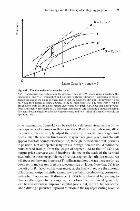
little imagination, figure 4.3 can be used for a different visualization of theconsequences of changes in these variables. Rather than redrawing all ofthe curves, one can simply adjust the scales by renormalizing wages andprices. Then the revenue function will stay in its original place, and OB willappear to rotate counterclockwise (up) through the first quadrant, perhapsto position, OD, as depicted in figure 4.4. A wage increase would reduce therents earned from f from the length of segment AB to that of CD. (Anoutput price decrease would involve a change in the scale of the verticalaxes, ruining the correspondence of vertical segment lengths to rents, so wewill focus on the wage increase.) This illustrates how a wage increase drivesdown rents and creates pressure to economize on labor. Note that CD is tothe left of AB. Faced with a wage increase, the firm will reduce the amountof labor and output slightly, raising average labor productivity, consistentwith what Cooper and Haltiwanger (1993) have observed happening toplants as they aged. In the long run, technological improvements generallylead to investments in improved capital goods that, in turn, bid for scarcelabor, driving a persistent upward rotation in the ray representing revenue


Fig. 4.4 The dynamics of a wage increaseNote: If wages rise relative to prices, the revenue � cost ray, OB, would remain fixed and thefunctions, f and f , g, would shift and elongate rightward. However, it is possible to renor-malize the axes in the plane as wages rise so that the functions stay put. The revenue � costray would then appear to rotate upward, to the position of ray OD. The rents from f will bedriven down from the length of segment AB to that of segment CD. Note that labor produc-tivity rises slightly (the slope of OC is greater than that of OA). Machine g meets a differentfate: rents become negative after the wage increase, and so it is shut off abruptly to avoid anoperating loss.

equals cost. The effect of obsolescence is just the rent lost due to the persis-tent rise in wages relative to the price of output. This rise (or rotation in rayOB) is not necessarily a constant—a cyclical downturn in the economy canaccelerate the upward rotation of the ray, while a surge in demand can tem-porarily reverse the process, causing a downward rotation of ray OB andan increase in rents. A key point is that the rotation of OB reflects both tem-poral and cyclical influences. The two exogenous influences tend to getswept together in the standard approach to capital measurement. The tem-poral influence creates obsolescence, while the cyclical influence is whatunderlies the Berndt and Fuss (1986) “temporary equilibria.”

4.4.3 Negative Rents, If Permanent, Will Induce Asset Retirement

Negative rents would occur if wages rose enough so that a revenue func-tion fell entirely below the revenue or cost ray, as is the case with g and rayOD in figure 4.4. Negative rents can occur if the revenue function has afixed labor requirement. No output (revenue) is produced unless this re-quirement is met, but once it is met, the function rises rapidly. If OD is highenough, and if diminishing marginal returns set in soon enough, revenuesmay never cover costs. Any attempt to operate the machine will result in aloss. In this situation, we assume that the machine is shut down. Unlike acapital stock, the machine model can be consistent with an abrupt shut-down of a machine or plant—as OB rises (and before it reaches OD), rentswould transition from positive to negative, causing all labor suddenly to bewithdrawn from the asset. This type of model could potentially be usedwith microdata to investigate plant closing behavior, but this paper will fo-cus on measuring capital.

In order to predict abrupt retirements, the machine model must be spec-ified with a fixed labor requirement as in my figures.2 This cannot happenwith the Cobb-Douglas specification3 of the vintage production functionthat Solow (1960) used in an empirical exercise. As depicted in figure 4.5,Solow’s functions would start at the origin and move out into the firstquadrant, with newer vintages above older. The slope of each curve wouldgradually decline, reflecting diminishing marginal returns to labor. Butthere would be diminishing average returns to labor throughout eachcurve. If the ray OB gradually rotated upward squeezing rents, the firmwould continue to operate the machine using less and less labor until laborreached zero. Falling rents would not lead to abrupt shutdowns, and, in-stead, old machines would just gradually fade away.

It is interesting that on any function, f, that has a region where labor pro-ductivity is rising, labor productivity will reach a maximum at the point at


2. This can happen with any specification with a region where average returns to labor (la-bor productivity) are rising.

3. Output per unit of capital, with the Solow’s vintage Cobb-Douglas function, is given by(Yt,v /Kt,v ) � Bev(Lt,v /Kt,v)

�.

which the curve is tangent to a ray from the origin. As a consequence of di-minishing marginal returns, a machine will never operate to the left of thispoint. It follows that the labor productivity associated with a machine is atits maximum when the machine is marginal. Machines will operate to theright of this point.

4.5 Measuring Real Capital

Given the machine model, we now consider what measurement unitsand weights would be suitable for the aggregation of real capital inputs.

4.5.1 Measurement Units and the Aggregation of Machines

The machine model can be used to devise an aggregate capital measurethat reflects many of the factors affecting capital vintages. This perspectivewill help to identify how these factors are being treated in recent studies ofcapital and productivity. The model includes a unit, the number of ma-chines, nt,v,m, that can be used to add up identical assets. This is a less con-strained starting point for vintage aggregation than the usual real value ofinvestment. However, each category of machine is different. Expression (4)


Fig. 4.5 Cobb-Douglas specificationNote: Solow mentioned one possible specification for his vintage production function, andhere it is graphed for two machines. Because there is no part of the domain where there are in-creasing average returns to labor, rents will only approach zero as wages become very high.Negative rents are impossible, and there is not an abrupt transition from operating with a lotof labor to being shut down. Old machines do not die, they just gradually fade away.

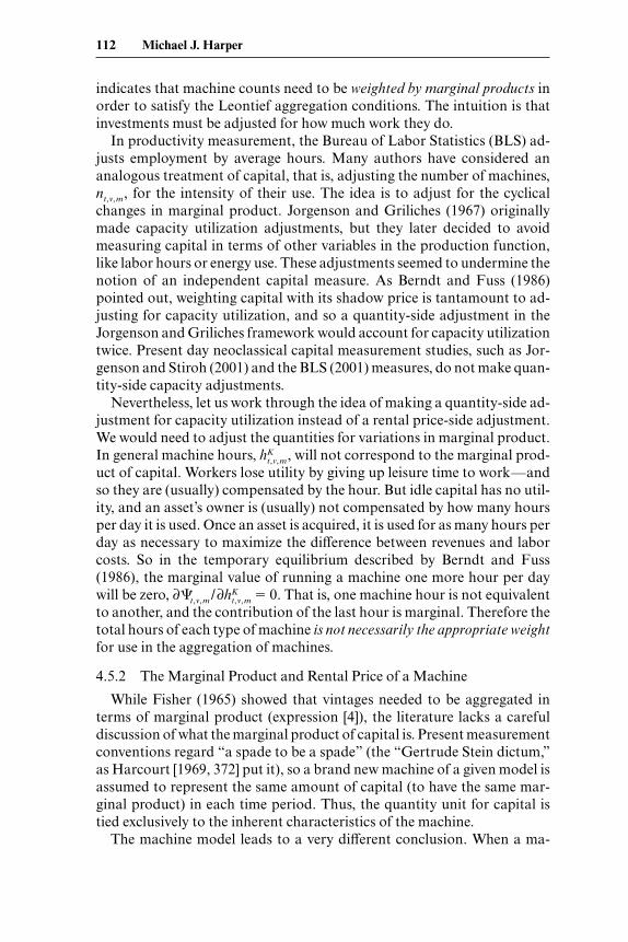
indicates that machine counts need to be weighted by marginal products inorder to satisfy the Leontief aggregation conditions. The intuition is thatinvestments must be adjusted for how much work they do.

In productivity measurement, the Bureau of Labor Statistics (BLS) ad-justs employment by average hours. Many authors have considered ananalogous treatment of capital, that is, adjusting the number of machines,nt,v,m, for the intensity of their use. The idea is to adjust for the cyclicalchanges in marginal product. Jorgenson and Griliches (1967) originallymade capacity utilization adjustments, but they later decided to avoidmeasuring capital in terms of other variables in the production function,like labor hours or energy use. These adjustments seemed to undermine thenotion of an independent capital measure. As Berndt and Fuss (1986)pointed out, weighting capital with its shadow price is tantamount to ad-justing for capacity utilization, and so a quantity-side adjustment in theJorgenson and Griliches framework would account for capacity utilizationtwice. Present day neoclassical capital measurement studies, such as Jor-genson and Stiroh (2001) and the BLS (2001) measures, do not make quan-tity-side capacity adjustments.

Nevertheless, let us work through the idea of making a quantity-side ad-justment for capacity utilization instead of a rental price-side adjustment.We would need to adjust the quantities for variations in marginal product.In general machine hours, hK

t,v,m, will not correspond to the marginal prod-uct of capital. Workers lose utility by giving up leisure time to work—andso they are (usually) compensated by the hour. But idle capital has no util-ity, and an asset’s owner is (usually) not compensated by how many hoursper day it is used. Once an asset is acquired, it is used for as many hours perday as necessary to maximize the difference between revenues and laborcosts. So in the temporary equilibrium described by Berndt and Fuss(1986), the marginal value of running a machine one more hour per daywill be zero, ∂�t,v,m /∂hK

t,v,m � 0. That is, one machine hour is not equivalentto another, and the contribution of the last hour is marginal. Therefore thetotal hours of each type of machine is not necessarily the appropriate weightfor use in the aggregation of machines.

4.5.2 The Marginal Product and Rental Price of a Machine

While Fisher (1965) showed that vintages needed to be aggregated interms of marginal product (expression [4]), the literature lacks a carefuldiscussion of what the marginal product of capital is. Present measurementconventions regard “a spade to be a spade” (the “Gertrude Stein dictum,”as Harcourt [1969, 372] put it), so a brand new machine of a given model isassumed to represent the same amount of capital (to have the same mar-ginal product) in each time period. Thus, the quantity unit for capital istied exclusively to the inherent characteristics of the machine.

The machine model leads to a very different conclusion. When a ma-


chine is added to the economy while total labor is held constant, the out-put of the new machine will be gained, but some output from other ma-chines will be lost because labor must be redeployed to the new machineand away from other machines.4 Because labor is always redeployed at la-bor’s marginal product, the new machine will boost output by the differ-ence of the average product of labor on this machine, and the marginalproduct of labor (which will be the same on the new machine as on all othermachines). Hence the marginal product of machines, zt,v,m � ∂Yt /∂nt,v,m, is

(16) zt,v,m � � � � � � .

The marginal product of the machine is determined by its own machineproduction function and by the marginal product of labor, which in turn isdetermined by the ratio of exogenous functions of time, wt /pt . Marginalproduct closely corresponds to rent. Rent per machine, or the machinerental price, ct,v,m, is just the price of output times the machine’s marginalproduct:

(17) ct,v,m � � ptzt,v,m

Note that, ct,v,m reflects the marginal product of capital in that differencesin marginal products between machines, z, will show up as differences inthe rental prices, c.

It is possible to picture how a machine’s marginal product changes byprojecting figure 4.4 back into the output–labor-hours plane of figure 4.1.Figure 4.6 depicts the rays OB and OD representing the two given wage-price ratios, projected into output-labor space. Marginal products are pro-portional to the vertical distances between each operating point and therelevant ray. As the wage-price ratio changes, the vertical distances associ-ated with different vintages will clearly change. If figure 4.6 depicted sev-eral functions like figure 4.2, it would be clear that the marginal productsof machines are affected disproportionately by variations in the exogenousprice of output and wage rate. In particular, rents and the marginal prod-

�t,v,m�nt,v,m

Lt,v,m�nt,v,m

∂Yt,v,m�∂Lt,v,m

Yt,v,m�Lt,v,m

∂Yt,v,m�∂Lt,v,m

Lt,v,m�nt,v,m

Yt,v,m�nt,v,m


4. An example may help. Suppose there are fifty identical machines in the economy, eachmachine using ten workers to make 100 units of output (500 workers and 5,000 units of out-put in all). If one more machine is added to the economy and ten more workers, 100 more unitsof output will be produced. But to compute the marginal product of capital, total labor mustbe held fixed, so ten of the fifty-one machines now must be operated with only nine workers.If these ten machines now produce only ninety-four units of output each, the net gain fromadding the fifty-first machine to the economy would be only forty units [100 – 10 � (100 – 94)].This marginal product will depend on how scarce labor is. Had we started instead by operat-ing the fifty machines with only seven laborers making eighty units of output each, the intro-duction of the fifty-first machine would require seven machines to be operated with six work-ers each, the seven machines producing perhaps only seventy units each. Then the marginalproduct of capital would be only ten units [80 – 7 � (80 – 70)]. The usefulness of another ma-chine is lower when labor is a relatively scarce resource.

ucts of older assets are affected proportionally more by cyclical effects and byobsolescence than are the rents and marginal products of newer more pro-ductive assets. The Leontief aggregation conditions require ratios of mar-ginal products among machines to be independent of exogenous variables.Capital stock measures impose this, at odds with how assets with differ-ences in productivity will behave.

4.5.3 The Rigid Homogeneity Assumption Underlying Capital Stock Measures

One possible arrangement of machine functions is of special signifi-cance. A group of machines, Gt,v,m, is defined to be homogeneous if, for anytwo functions, fi, j,k and ft,v,m ⊂ Gt,v,m there exists an �i, j,k such that:

(18) fi, j,k(�i, j,kL) � �i, j,k ft,v,m(L) ∀ L.

Fisher (1965) and Hall (1968) used different proofs to show that vintagesmust be homogeneous in order for the vintage aggregate, J, to exist. Figure4.7 illustrates the similarity of machine functions for a homogeneousgroup of machines. For any given pt /wt ratio, all machines will operate withthe same proportions of output and labor, that is, the same labor produc-tivity. One function is never strictly above another like in figure 4.2, that is,


Fig. 4.6 The marginal product of a machineNote: Rays OB and OD in figure 4.4 can be projected back into output–labor-hours plane offigure 4.1. Segments AB and CD then represent the marginal product of the machine beforeand after the wage increase. Even though the machine is exactly the same, the marginal prod-uct of the machine is driven down by an increase in wages because the opportunity cost of la-bor (the output the worker could make with some other machine) has risen. In the long run,technical change and investments in efficient assets drive a steady upward rotation of the ray.

one machine will never produce more output than another with the samelabor. It is clear that two machines are not homogeneous if one of them em-bodies an improvement that enhances labor productivity. Nor can an oldermachine, whose machine production function has deteriorated, be part ofthe same homogeneous class as a new machine.

Within a homogeneous group, machines can produce different amountsof output with proportionally different amounts of labor input. Call thevalue of �i, j,k that satisfies expression (18) the size of machine i, j, k com-pared to machine t, v, m. A new machine can be bigger but not better. Im-posing a homogeneity assumption is implausible and inappropriate if oneis interested in measuring high technology capital and characterizing thesources of growth. Yet such homogeneity is assumed in capital stock mea-surement.

What are the consequences of assuming homogeneity? The fixed age-efficiency schedule is at odds with the fact that relative marginal productswill vary by vintage. The fixed schedule imposes homogeneity, as defined byequation (18) on the vintage machine production functions. All vintagesare assumed to be affected proportionally by a demand shock. In effect,vintage machines are assumed to differ only in size. To the extent that as-


Fig. 4.7 A family of homogeneous machine functionsNote: The Leontief aggregation conditions fail unless the relative marginal products of ma-chines are unaffected by the rotation of ray OB. Machines with higher potential labor pro-ductivity than others (like in figure 4.2) are ruled out of a homogeneous group. Machines canbe bigger but not better. This is unsuitable for studying technologically improved equipment,but it is what economists assume in measuring capital stock.

sets actually differ in labor productivity, as in figure 4.2, any exogenousshock should actually affect the marginal products of the oldest and leastefficient vintages proportionally more than those of the newer ones. Be-cause of the built-in homogeneity assumption, capital stocks can lead topuzzling results when used in short-run models, such as those reported byBrynjolfsson and Hitt (2003).

An age-efficiency function could be constructed to correct for any steadyand persistent temporal influence such as obsolescence, as Wykoff (2003)has suggested. In this case, the age-efficiency function is adjusted for theeffects on marginal product of obsolescence (the upward rotation of rayOA, as in figure 4.6) as well as the effects of deterioration in the function f.However it is clear that a time-invariant–age-efficiency function will beunable to correct for cyclical influences. The idea of a capacity utilizationadjustment is to correct for this problem. However, a capacity utilizationratio for the capital stock will not accurately model the myriad vintage-specific adjustments to marginal products brought about by a cyclicalchange in demand. Ideally, a separate capacity adjustment would be cal-culated for each vintage. The vintage aggregate capital service measurewould then be the sum across vintages of investments adjusted for capac-ity effects, as well as for deterioration and obsolescence.

4.6 Measuring Quality Change

In the literature on quality adjustment of consumer goods, it is ax-iomatic that relative prices reflect relative utilities. In measuring inputs as-sociated with durable capital goods, the usual assumption is that relativegoods prices measure relative marginal products. My point of departure isthat they do not.

Triplett (1989) recognized that rental prices rather than purchase pricesshould be used to compare marginal products. In neoclassical theory, thepurchase price of an asset presumably equals the discounted value of its fu-ture rents. The ratio of purchase prices of two assets is therefore propor-tional to the ratio of their discounted streams of future rents and not nec-essarily to the ratio of marginal products. At first blush, it seems modest toassume the rental streams will be proportional to marginal products, en-suring that the purchase prices are in step with the rental prices. After all,such proportionality will occur if age-efficiency functions are geometric.

But if new machines embody technical change, that is, if the labor pro-ductivity associated with newer models is higher, and if the machine func-tions contain regions of increasing returns to labor (such as is the case ifthere is a fixed labor requirement for each machine), then obsolescence willpush down rents of older models proportionately faster than rents of newermodels. Because of this, the ratio of the price of a more productive modelto that of a less productive model will overstate the ratio of marginal prod-


ucts. As Hulten (1992) noted, the notion of capital quality is grounded inHall’s (1968) embodiment factor, which itself describes aggregation withmarginal products.

4.6.1 Obsolescence, the Functional Form of Marginal Product with Age, and Quality Change

Observations of purchase prices, whether determined with hedonic ormatched-model techniques, are required to measure quality. But informa-tion on the functional pattern by which obsolescence affects marginalproducts as models age also is required. For example, assume that modelsare impacted as they age by obsolescence, but not by deterioration. Olinerand Sichel (2000) contend that obsolescence dominates deterioration incontributing to a high-tech asset’s demise. Further, assume that wt /pt ro-tates upward at a steady rate without cyclical disturbances. Processes, suchas quality improvements, are then presumed to occur at fixed rates so thatthe quality of a new model, in any year t, relative to one introduced oneyear earlier will be Bt � zt,t,t /zt,t,t–1. Let � be the age(�)/efficiency function,i.e. � � zt,t,t–� /zt,t,t. Under the assumptions, Bt � 1/ 1. From the neoclassi-cal axiom that the price of an asset equals the discounted future rents, onecan determine the price of a new model relative to last year’s model:

(19) � �

If quality raises the labor productivity of newer models, (which it must doif there is a technological improvement as distinct from an increase in size),rents, p , will be forced down by obsolescence proportionally faster withage, i.e. d 2 ln � /d�2 � 0, and the machine will eventually be retired, that is, � � 0 for � � L. Under these conditions the ratio of integrals on the right-hand side of expression (19) will be greater than one. The ratio of modelprices will exceed relative quality.

The bias in the existing durable goods quality adjustments is likely to besubstantial. Figure 4.8 plots the marginal products of hypothetical goods.For example, computers could be depicted by straight-line–age-efficiencyfunctions with short lives. The age-efficiency functions decline because ofthe temporal effects of a steady increase in wt /pt. Newer models embodytechnical improvements. The relative marginal product of a newer modelto that of an older one at any time would be proportional to the ratio ofheights of the lines in left-hand-side portion of figure 4.8. The relative as-set prices will be proportional to a ratio involving areas. Thus, the area un-der each line, from a given time through the rest of the life of the asset, willrepresent the asset’s (nondiscounted) future rents. If the discount rate iszero and the effects of obsolescence are straight-line, as in figure 4.8, qual-

Bt ��

u�0pt�u ue

�rudu��

u�0pt�u( u�1/ 1)e�rudu

��

u�0pt�u ue

�rudu��

u�0pt�u u�1e

�rudu

pKt,t,t

�pK

t,t,t�1


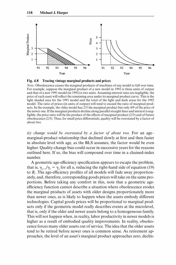
ity change would be overstated by a factor of about two. For an age–marginal-product relationship that declined slowly at first and then fasterin absolute level with age, as the BLS assumes, the factor would be evenhigher. Quality-change bias could occur in successive years for the reasonsoutlined here. If so, the bias will compound over time in a chained-indexnumber.

A geometric age-efficiency specification appears to escape the problem,that is, u�1/ 1 � u for all u, reducing the right-hand side of equation (19)to Bt. The age-efficiency profiles of all models will fade away proportion-ately, and, therefore, corresponding goods prices will take on the same pro-portions. Before taking any comfort in this, note that a geometric age-efficiency function cannot describe a situation where obsolescence erodesthe marginal products of assets with older designs proportionately morethan newer ones, as is likely to happen when the assets embody differenttechnologies. Capital goods prices will be proportional to marginal prod-ucts only if the geometric model really describes events at the microlevel,that is, only if the older and newer assets belong to a homogeneous family.This will not happen when, in reality, labor productivity in newer models ishigher as a result of embodied quality improvements. In reality, obsoles-cence forces many older assets out of service. The idea that the older assetstend to be retired before newer ones is common sense. As retirement ap-proaches, the level of an asset’s marginal product approaches zero, declin-


Fig. 4.8 Tracing vintage marginal products and pricesNote: Obsolescence causes the marginal products of machines of any model to fall over time.For example, suppose the marginal product of a new model in 1992 is three units of outputand that of a new 1991 model (in 1992) is two units. Assuming interest rates are negligible, theprice of each asset will reflect the remaining area under its marginal product curve. This is thelight shaded area for the 1991 model and the total of the light and dark areas for the 1992model. The ratio of prices (in units of output) will tend to exceed the ratio of marginal prod-ucts. In the example, the older model has 2/3 the marginal product but only 4/9 of the price ofthe newer one. If the marginal products decline along parallel straight lines and interest is neg-ligible, the price ratio will be the product of the effects of marginal product (2/3) and of futureobsolescence (2/3). Thus, for small price differentials, quality will be overstated by a factor ofabout two.

ing faster and faster in percentage terms. Hence Bt must be greater than 1.By assuming that Bt � 1, consistent with a geometric model, the standardapproach to quality adjustment disregards key evidence.

4.7 Summary

Capital stock measures are widely used in the economics literature. Cap-ital stocks are constructed from data on vintage investment by means ofstrong aggregation assumptions. It is assumed that the capital services ofvintage investments are predetermined and that they decay with age, inde-pendent of prevailing wages and output prices. These assumptions wereidentified as a potential limitation in the 1950s. Mechanisms have been de-veloped to adjust capital stocks for the manifestations of these rigid as-sumptions. Capacity utilization adjustments to capital stocks account forcyclical variations in output, while quality adjustments are made to invest-ments to correct for temporal improvements in the technology embodiedin capital goods. Like capital stocks, however, these measurement adjust-ments involve strong assumptions. This has been recognized for decadesin the case of capacity utilization. In the case of quality, the potential forbias may be underappreciated. I hope that this paper helps raise awarenessof these issues and their importance to our understanding of economicgrowth.

References

Berndt, Ernst R., and Melvyn A. Fuss. 1986. Productivity measurement with ad-justments for variations in capacity utilization and other forms of temporaryequilibrium. Journal of Econometrics 33 (1/2): 7–29.

Brynjolfsson, Erik, and Lorin M. Hitt. 2003. Computing productivity: Firm-levelevidence. Review of Economics and Statistics 85 (4): 793–808.

Bureau of Labor Statistics. 2001. Multifactor productivity trends, 1999. U.S. De-partment of Labor News Release no. 01-125, May 3, 2001.

Cooper, Russell, and John Haltiwanger. 1993. The aggregate implications of ma-chine replacement: Theory and evidence. American Economic Review 83:360–82.

Fisher, Franklin M. 1965. Embodied technical change and the existence of an ag-gregate capital stock. Review of Economic Studies 32:263–88.

Griliches, Zvi. 1963. Capital stock in investment functions: Some problems of con-cept and measurement. In Measurement in economics, ed. Carl Christ. Stanford,CA: Stanford University Press. Repr. in Technology, education and productivity,ed. Zvi Griliches, 123–43. New York: Basil Blackwell, 1988.

Hall, Robert E. 1968. Technical change and capital from the point of view of thedual. Review of Economic Studies 35 (January): 35–46.

Harcourt, G. C. 1969. Some Cambridge controversies in the theory of capital. Jour-nal of Economic Literature 7 (2): 369–405.

Hill, Peter. 2000. Economic depreciation and the SNA. Paper presented at the 26th


conference of the International Association for Research in Income and Wealth,Cracow, Poland.

Hulten, Charles R. 1992. Growth accounting when technical change is embodiedin capital. American Economic Review 82 (4): 964–79.

———. 2001. Total factor productivity: A short biography. In New developments inproductivity analysis, ed. Charles R. Hulten, Edwin R. Dean, and Michael J.Harper, 1–47. Chicago: University of Chicago Press.

Jorgenson, Dale W., and Zvi Griliches. 1967. The explanation of productivitychange. Review of Economic Studies 34 (3): 249–82.

Jorgenson, Dale W., and Kevin J. Stiroh. 2001. Raising the speed limit: U.S. eco-nomic growth in the information age. Brookings Papers on Economic Activity, Is-sue no. 1:125–235. Washington, DC: Brookings Institution.

Leontief, Wassily W. 1947. Introduction to a theory of the internal structure offunctional relationships. Econometrica 15:361–73.

Morrison, Catherine J., and Ernst R. Berndt. 1981. Short-run labor productivity ina dynamic model. Journal of Econometrics 16:339–65.

Oliner, Stephen D., and Daniel E. Sichel. 2000. The resurgence of growth in the late1990s: Is information technology the story? Journal of Economic Perspectives 14(4): 3–22.

Solow, Robert M. 1957. Technical change and the aggregate production function.Review of Economics and Statistics 39 (3): 312–20.

———. 1960. Investment and technical progress. In Mathematical methods in thesocial sciences, ed. K. Arrow, S. Karlin, and P. Suppes, 339–65. Stanford, CA:Stanford University Press.

———. 2001. After technical progress and the aggregate production function. InNew developments in productivity analysis, ed. Charles R. Hulten, Edwin R.Dean, and Michael J. Harper, 173–78. Chicago: University of Chicago Press.

Triplett, Jack E. 1989. Price and technological change in a capital good: A surveyof research on computers. In Technology and capital formation, ed. Dale W. Jor-genson and Ralph Landau, 127–213. Cambridge, MA: MIT Press.

Wykoff, Frank C. 2003. Obsolescence in economic depreciation from the point ofview of the revaluation term. Paper presented at the NBER Summer Institute’sConference on Research in Income and Wealth, Cambridge, MA.


Technology and the Theory of Vintage Aggregation - National

Documents

Transcript of Technology and the Theory of Vintage Aggregation - National