TECHNOLOGY AND GREENHOUSE GAS EMISSIONS: …LBNL-42054 UC-000 EPA 430-R-98-021 TECHNOLOGY AND...

LBNL-42054UC-000

EPA 430-R-98-021

TECHNOLOGY AND GREENHOUSE GAS EMISSIONS:AN INTEGRATED SCENARIO ANALYSIS

USING THE LBNL-NEMS MODEL

Jonathan G. Koomey, R. Cooper Richey, Skip Laitner,Robert J. Markel, and Chris Marnay

Energy Analysis DepartmentEnvironmental Energy Technologies Division

Ernest Orlando Lawrence Berkeley National LaboratoryUniversity of California

Berkeley, CA 94720

and

United States Environmental Protection AgencyOffice of Atmospheric Programs

Washington, DC 20401

http://enduse.lbl.gov/Projects/GHGcosts.html

September 1998

This work was supported by the Office of Atmospheric Programs of the U.S. Environmental ProtectionAgency. Prepared for the U.S. Department of Energy under Contract No. DE-AC03-76SF00098.

EXECUTIVE SUMMARY

The common perception among many policy makers and industry leaders is that the twinobjectives of reducing greenhouse gas emissions and promoting a more competitiveeconomy are inherently contradictory. Many believe that anything done to lower suchemissions will necessarily restrict economic activity. Others argue that if the economymoves forward at current levels of efficiency, growth in greenhouse gas emissions will beinevitable and the global climate will be seriously damaged. Because of the "unavoidabletradeoff" between these two objectives, the various industry, government andenvironmental groups wage a constant policy battle over which objective merits the greatersupport. From a perspective of cost-effective investments in technology, however, itbecomes increasingly clear that these two goals are not at all contradictory. The reason isthat the U.S. economy falls short of an optimal level of overall carbon efficiency.

Figure ES-1 on the following page illustrates the different points of view in a schematicway. The curves on this graph represent different "Production Possibility Frontiers" thatcharacterize the relationship between carbon emissions mitigation and economic activity.The frontier defines the outer boundary of what is feasible given a set of technologies andeconomic activity levels.

Most modeling of the costs of reducing carbon emissions assumes that the reference casecarbon intensity is on the frontier, and that any increase in carbon mitigation must alsoresult in a decrease in Gross Domestic Product (this point of view corresponds to the curvelabeled "Assumed Year 2010 Business-As-Usual Case Frontier"). Our analysisdemonstrates that the "Actual Year 2010 Business-As-Usual Case Frontier" is further outthan the assumed frontier, which means that both carbon mitigation and GDP can beincreased at the same time, given the right set of policies and programs. In addition, sincethe frontier is a function of technology, and the cost of that technology is a function ofpolicy choices made between now and 2010, taking aggressive actions now to reducecarbon emissions can actually move the frontier further out than it would be given thetechnologies that exist in the reference case. This possibility is represented by the curvelabeled "Year 2010 Aggressive Implementation Case Frontier".

This report describes an analysis of possible technology-based scenarios for the U.S.energy system that would result in both carbon savings and net economic benefits. We usea modified version of the Energy Information Administration's National Energy ModelingSystem (LBNL-NEMS) to assess the potential energy, carbon, and bill savings from aportfolio of carbon saving options. This analysis is based on technology resourcepotentials estimated in previous bottom-up studies, but it uses the integrated LBNL-NEMSframework to assess interactions and synergies among these options.

The U.S. economy now emits 192 grams of carbon for each dollar of value-added(measured as GDP in constant 1996 dollars) that it produces. With a "normal" rate ofimprovement in the Business-As-Usual case, it appears that by the year 2010, the nationwould reduce this emissions rate to about 170 grams per dollar. Despite this improvementin the emissions rate, however, the anticipated growth in the economy will increase totalcarbon emissions to 1803 MtC in 2010, or to about 23 percent above 1996 levels.

The LBNL-NEMS analysis conducted in this study suggests that implementing a set ofpolicies to encourage the development and deployment of energy-efficient and low-carbontechnologies can close this gap — to the benefit of both the climate and the economy. Inthis study, we find a cost-effective path that can reduce the rate of carbon emissions to 147grams per dollar of GDP. This will reduce carbon emissions to about 1530 MtC by 2010.

i

Other studies suggest that with the right mix of policies and technologies, the frontier mightactually extend well beyond that described in this report (ASE et al. 1997, Brown et al.1998, Interlaboratory Working Group 1997, Krause 1996, Laitner et al. 1998).

The High-Efficiency Low Carbon scenario analyzed in this study would result insignificant annual net savings to the U.S. economy, even after accounting for all relevantinvestment costs and program implementation costs. This strategy would result in roughlyhalf of the carbon reductions needed to meet the Kyoto target being achieved from domesticU.S. investments. Not pursuing this technology-led investment strategy would have anopportunity cost of more than $50B per year for the U.S. in 2010 and more than $100Bper year by 2020.

Figure ES-1: Schematic production possibility frontiers

Carbon Intensity

Current U.S. ~192 g/1996$

2010 EIA AEO98 Business-As-Usual Case ~170 g/1996$

2010 LBNL-NEMS High Efficiency Low Carbon Case ~147 g/1996$

Level ofCarbon

Mitigation

Gross Domestic Product

Actual Year 2010Business-As-Usual

Case Frontier

Year 2010Aggressive Implementation

Case Frontier

Assumed Year 2010Business-As-Usual

Case Frontier

ii

PREFACE

The U.S. Environmental Protection Agency (EPA) has a long history of examining the roleof technology in strengthening both the nation’s environmental quality and overalleconomic activity. Following that same path, EPA’s Office of Atmospheric Programs(OAP) has initiated a number of analytical exercises to explore opportunities for reducingthe emission of greenhouse gases through cost-effective investments in energy-efficiencyand renewable energy technologies. This report builds on one set of results from thislarger effort.

The work reviewed in this report was made possible through EPA funding of the E.O.Lawrence Berkeley National Laboratory (LBNL). In undertaking the assignment, LBNLwas specifically asked to evaluate how different assumptions about technology diffusionmight affect the opportunity for cost-effective reductions of energy-related carbonemissions. The analysis was primarily conducted by Jonathan G. Koomey and CooperRichey (LBNL) under the overall guidance of EPA’s Skip Laitner (who also suppliedsignificant amounts of text). In addition, Robert Markel and Chris Marnay of LBNLcontributed to the research leading up to the publication of this report.

This report benefited from the contributions of a peer review panel. Their extensivecomments are summarized in the appendix of this report, together with an indication ofhow we incorporated their suggestions into our analysis. Indeed, the comments of thereview panel, together with our own thoughts in response to those comments, may providea valuable background document for those interested in the climate change issue.

The members of the peer review panel (in alphabetical order) who generously shared theirinsights with us include:

Dr. Stephen Bernow, Tellus InstituteBoston, MA

Dr. Stephen DeCanio, University of California-Santa BarbaraSanta Barbara, CA

Dr. Neal Elliott, American Council for an Energy-Efficient EconomyWashington, DC

Dr. Eban Goodstein, Lewis and Clark CollegePortland, OR

Dr. Julie Fox Gorte, Northeast-Midwest InstituteWashington, DC

Dr. Lorna Greening, Economic ConsultantBoulder, CO

Dr. Bruce Hutton, University of DenverDenver, CO

Dr. Florentin Krause, International Project for Sustainable Energy PathsEl Cerrito, CA

Dr. Andy Kydes, EIA Office of Integrated Analysis and Forecasting

iii

Washington, DC

Dr. James E. McMahon, Lawrence Berkeley National LaboratoryBerkeley, CA

Dr. Alan H. Sanstad, Lawrence Berkeley National LaboratoryBerkeley, CA

Dr. Thomas Tietenberg, Colby CollegeWaterville, ME

Dr. Michael Toman, Resources for the FutureWashington, DC

Dr. Frances Wood, On Location, Inc.Dunn Loring, VA

The listing of individual affiliation for each of our review panel members is foridentification purposes only. Although we gladly acknowledge the involvement of theindividual members of the peer review panel, we do not mean to imply their endorsementof this report. The final responsibility for the results of the analysis and the content of thereport lies solely with the authors.

This work was supported by the Office of Atmospheric Programs of the U.S. Environmental ProtectionAgency. Prepared for the U.S. Department of Energy under Contract No. DE-AC03-76SF00098.

iv

TABLE OF CONTENTS

Executive Summary . . . . . . . . . . . . . . . . . . . . . . . . . . . . . . . . . . . . . . . . . . . . . . . . . . . . . . . . . . . i

Preface . . . . . . . . . . . . . . . . . . . . . . . . . . . . . . . . . . . . . . . . . . . . . . . . . . . . . . . . . . . . . . . . . . . . . . . . . iii

I n t r o d u c t i o n . . . . . . . . . . . . . . . . . . . . . . . . . . . . . . . . . . . . . . . . . . . . . . . . . . . . . . . . . . . . . . . . . . . . 1Analytical objectives of this study ... . . . . . . . . . . . . . . . . . . . . . . . . . . . . . . . . . . . . . . . . . . . . . . . . . . .3Incomplete technology portfolio .. . . . . . . . . . . . . . . . . . . . . . . . . . . . . . . . . . . . . . . . . . . . . . . . . . . . . . .3

M e t h o d o l o g y . . . . . . . . . . . . . . . . . . . . . . . . . . . . . . . . . . . . . . . . . . . . . . . . . . . . . . . . . . . . . . . . . . . 4The scenario approach....................................................................4Demand side...............................................................................5Supply side........ . . . . . . . . . . . . . . . . . . . . . . . . . . . . . . . . . . . . . . . . . . . . . . . . . . . . . . . . . . . . . . . . . . . . . . . .7Combined scenarios......................................................................9Investment costs .. . . . . . . . . . . . . . . . . . . . . . . . . . . . . . . . . . . . . . . . . . . . . . . . . . . . . . . . . . . . . . . . . . . . . . . . .9The programs-based perspective........................................................10

Results . . . . . . . . . . . . . . . . . . . . . . . . . . . . . . . . . . . . . . . . . . . . . . . . . . . . . . . . . . . . . . . . . . . . . . . . . 11Primary energy use.......................................................................11Carbon emissions.........................................................................14Power plant retirements..................................................................14Energy bill savings ... . . . . . . . . . . . . . . . . . . . . . . . . . . . . . . . . . . . . . . . . . . . . . . . . . . . . . . . . . . . . . . . . . . . .14Investment and program implementation costs........................................16Impact on the Nation’s Economy.......................................................16

Discussion . . . . . . . . . . . . . . . . . . . . . . . . . . . . . . . . . . . . . . . . . . . . . . . . . . . . . . . . . . . . . . . . . . . . . 18The importance of "hard-wired" end-uses and technologies.........................18Implementing technological change.....................................................19Understanding power plant retirements................................................19Effect of integrated analysis .. . . . . . . . . . . . . . . . . . . . . . . . . . . . . . . . . . . . . . . . . . . . . . . . . . . . . . . . . . . .19

F u t u r e w o r k . . . . . . . . . . . . . . . . . . . . . . . . . . . . . . . . . . . . . . . . . . . . . . . . . . . . . . . . . . . . . . . . . . . . 20Additional carbon saving options.......................................................20Better treatment of currently analyzed carbon saving options .... . . . . . . . . . . . . . . . . . . .20Improvements in synergy index.........................................................20Power plant efficiency....................................................................21Macroeconomic effects in NEMS.......................................................21Review of gas supply and demand interactions.......................................22Regional distribution of hydroelectric refurbishment capacity.......................22

C o n c l u s i o n s . . . . . . . . . . . . . . . . . . . . . . . . . . . . . . . . . . . . . . . . . . . . . . . . . . . . . . . . . . . . . . . . . . . . 22

References . . . . . . . . . . . . . . . . . . . . . . . . . . . . . . . . . . . . . . . . . . . . . . . . . . . . . . . . . . . . . . . . . . . . . 24

v

Appendix A: Technical Description of LBNL-NEMS High-EfficiencyLow Carbon Case . . . . . . . . . . . . . . . . . . . . . . . . . . . . . . . . . . . . . . . . . . . . . . . . . . . . . . . . . . . . . 27

A.1 All sectors .. . . . . . . . . . . . . . . . . . . . . . . . . . . . . . . . . . . . . . . . . . . . . . . . . . . . . . . . . . . . . . . . . . . . . . . . . . .27A.2 Electric utility sector................................................................29A.3 Residential sector .. . . . . . . . . . . . . . . . . . . . . . . . . . . . . . . . . . . . . . . . . . . . . . . . . . . . . . . . . . . . . . . . . .31A.4 Commercial sector..................................................................34A.5 Industrial sector.....................................................................36A.6 Transportation sector................................................................41

Appendix B: Complete List of LBNL-NEMS High-Efficiency/LowC a r b o n C a s e s . . . . . . . . . . . . . . . . . . . . . . . . . . . . . . . . . . . . . . . . . . . . . . . . . . . . . . . . . . . . . . . . . . 47

Appendix C: Summaries of key review comments. . . . . . . . . . . . . . . . . . . . . . . . . 49

Appendix D: Key outputs from selected modeling runs.. . . . . . . . . . . . . . . . . . 53

vi

LIST OF FIGURES

Figure ES-1: Schematic production possibility frontiers.....................................ii

Figure 1: Schematic representation of the NEMS modeling system .... . . . . . . . . . . . . . . . . . . . .2

Figure 2: Energy/GDP ratio over time, historical and projected.............................13

LIST OF TABLES

Table 1a: Primary energy and carbon results from LBNL-NEMS runs in 2010 ..........12

Table 1b: Primary energy and carbon results from LBNL-NEMS runs in 2020..........12

Table 2a: Energy bill savings results from LBNL-NEMS runs in 2010....................15

Table 2b: Energy bill savings results from LBNL-NEMS runs in 2020 ....... . . . . . . . . . . . .15

Table 3a: Summary of costs of energy services in 2010 (B1996$/year) ...... . . . . . . . . . . . . .17

Table 3b: Summary of costs of energy services in 2020 (B1996$/year)...................17

Table A.2.1 Coal plant retirement level criteria................................................29

Table A.3.1 Five Lab Study residential sector energy efficiency site energy savings(Quadrillion Btu)...................................................................................31

Table A.3.2 Residential sector annual average adjusted growth rates in theelectricity "other" category........................................................................33

Table A.4.1 Five Lab Study commercial sector energy efficiency site energysavings (Quadrillion Btu).........................................................................34

Table A.4.2 Commercial sector annual average adjusted growth rates in theelectricity "other" category........................................................................35

Table A.5.1 Retirement rates in the EIA AEO98 Hi-Tech case and LBNL-HEMSHELC case..........................................................................................36

Table A.5.2 ENPINT modifiers in the EIA AEO98 Hi-Tech case and LBNL-NEMS HELC case.................................................................................37

Table A.5.3 TPC parameters in the EIA AEO98 Hi-Tech case and LBNL-NEMSHELC case..........................................................................................37

Table A.5.4 Energy efficiency savings predicted by the LIEF model andimplemented in the LBNL-NEMS High Efficiency case......................................38

Table A.6.1 Technology parameters we modified in the cffuel file.........................42

vii

Table A.6.2 Technology parameters* we modified by technology in the cffuel fileby truck category...................................................................................42

Table A.6.3 Technology parameters we modified.............................................43

Table A.6.4 Technology parameters* we modified by technology by car and lighttruck category ... . . . . . . . . . . . . . . . . . . . . . . . . . . . . . . . . . . . . . . . . . . . . . . . . . . . . . . . . . . . . . . . . . . . . . . . . . . . . . . . . . . .44

Table A.6.5 Technology marketshares we modified by marketshare type, vehiclegroup, and size class .. . . . . . . . . . . . . . . . . . . . . . . . . . . . . . . . . . . . . . . . . . . . . . . . . . . . . . . . . . . . . . . . . . . . . . . . . . . . .45

Table D-1: LBNL-NEMS High-Efficiency/Low Carbon Cases in 2010, All-SectorForecast Summary.................................................................................54

Table D-2: LBNL-NEMS High-Efficiency/Low Carbon Cases in 2020, All-SectorForecast Summary.................................................................................56

Table D-3: Summary of Fuel Consumption by Sector for Selected Scenarios UsingLBNL-NEMS....................... ...............................................................58

viii

INTRODUCTION

The Kyoto protocol was a watershed event in the history of environmental policy. Foronly the second time in history, national governments have agreed to seek binding targetsfor pollutants that have global effects. If the U.S. decides to ratify the treaty and meet thesetargets, it will need to achieve aggressive reductions of greenhouse gas emissions in the2008 to 2012 time frame.

While many analyses have attempted to assess the potential costs of such a commitment,the debate is now shifting in a subtle way. An increasing number of business leaders andpolicy analysts are instead asking the question: "What are the key policy choices that mightactually enhance our industrial competitiveness and still lead to a significant reduction ofgreenhouse gas emissions?" Critical to this policy perspective is an investment-leddeployment of cost-effective technology that can both save money and reduce suchemissions.

Unfortunately, none of the existing policy models have successfully incorporated a fullrange of technological change within their analytical framework. In other words, suchmodels understate the opportunity for widely-available but underutilized and cost-effectivetechnologies to reduce greenhouse gas emissions. Nor do they anticipate or allow newtechnologies to emerge in response to changing conditions in the marketplace. Hence,much of the modeling response to any given climate change strategy reflects a more limitedtechnical capacity to respond positively to changing price signals, non-price policyinitiatives, and economic conditions. For that reason, there is a need: (a) to identify thebroader range of possible technological change through off-line analysis; and (b) to capturethe magnitude and direction of technological change within existing policy models toevaluate the potential economic impacts, using a scenario-based approach.

Developing a wide range of alternative technology scenarios can help us better understandthe ordinary business of making better choices with respect to both the environment and theeconomy. In the words of Kenneth Boulding: "Images of the future are the keys to choice-oriented behavior." For this reason, the analysis in this paper builds on previous estimatesof possible “technology paths” to investigate four major components of an aggressivegreenhouse gas reduction strategy:

(1) the large scale implementation of demand-side efficiency, comparable in scale tothat presented in two recent policy studies on this topic;

(2) a variety of "alternative" electricity supply-side options, including biomass cofiring,extension of the renewables production tax credit for wind, increased industrialcogeneration, and hydropower refurbishment.

(3) the economic retirement of older and less efficient existing fossil-fired power plants;and

(4) a permit charge of $23 per metric ton of carbon (1996$/t),1 assuming that carbontrading is implemented in the US, and that the carbon permit charge equilibrates atthis level. This level of carbon permit charge, as discussed later in the report, is inthe likely range for the Clinton Administration's position on this topic.

1In this paper, all monetary figures are in constant 1996 dollars, unless otherwise specified. All referencesto tons of carbon are to metric tons.

1

These four options are important contributors to large carbon reductions identified in theso-called "Five Lab study" released in the fall of 1997. The extensive engineering andeconomic analysis contained in the 1997 study suggested that cost-effective technologiescould reduce carbon emissions by as much as 390 million metric tons (MtC) by 2010 at apermit price of $50/tC (Interlaboratory Working Group 1997). Perhaps more important forthis analysis is that both the Five Lab study assumptions and each of the four optionsreferenced above can be represented in the U.S. Department of Energy's (US DOE's)National Energy Modeling System (NEMS) in an accurate and conceptually clear way.Integrating the various technology assumptions within the NEMS framework allows us tocapture dynamic feedbacks, particularly those between energy demand and prices.

NEMS is an all-sector, integrating model of the US energy system that is exemplary for itscomprehensive treatment of supply-side technologies (particularly in the electricity sector)and its detailed treatment of energy demand at the end-use level (see Figure 1).

Figure 1: Schematic representation of the NEMS modeling system

Oil and gas supply module

Natural gas transmission and

distribution module

Coal market module

Renewable fuels module

Supply

Electricity market module

Petroleum market module

Residential demand module

Commercial demand module

Transportation demand module

Industrial demand module

DemandConversion

Macroeconomic activity module

International energy module

Integrating module

Adapted from US DOE (1998b).

2

We rely on a modified version of the NEMS model2 as an accounting tool, but also tocapture the income, price, and intersectoral effects on both energy demand and fuel prices.Such interactions are treated exogenously in most bottom-up studies. We set out todetermine whether an endogenous treatment within the LBNL-NEMS framework wouldalter the main conclusions of such studies.

Analytical objectives of this study

The goals of this analysis are twofold. The first is to generate scenarios using LBNL-NEMS to explore the effects of aggressive but cost-effective US effort to implement certaindemand and supply-side technologies that reduce greenhouse gas emissions. The second isto investigate synergies and interactions between demand and supply-side options to derivelessons for policy. An integrating model such as LBNL-NEMS is particularly useful forsuch explorations.

Our analysis parallels at least two previous efforts undertaken by the Energy InformationAdministration (EIA) itself. In both 1996 and 1997, EIA analysts examined the effect ofaccelerated technological change on the U.S. energy markets (Boedecker et al. 1996,Kydes 1997). While the two previous EIA reports offer an important step forward withrespect to understanding the role of technological progress within an energy and economicframework, the scenarios in this study differ in two ways.

First, in these earlier studies, the EIA analysts made less-detailed assumptions abouttechnological progress than done for the Five-Lab study, for example. For instance, withinthe industrial model EIA assumed that the annual rate of change in energy intensity woulddecline by about 1.4% compared to the reference case forecast of 1.0%. In our analysis werelied on the Long-Term Industrial Energy Forecast (LIEF) model (Ross et al. 1993) andthe Five-Lab Study to define cost-effective reductions in energy intensity (InterlaboratoryWorking Group 1997). Second, the EIA analyses were independent of any real policyscenarios while our analysis builds upon the kind of technological progress and behavioralchanges one might expect to see in a post-Kyoto world. Indeed, many of the policyoptions that might drive the kind of technological changes envisioned in the Five-Lab studyare now in various stages of review by the Administration and Congress (Laitner 1998).

Incomplete technology portfolio

This analysis, because of time constraints, implemented an incomplete portfolio of carbonreduction options. For example, the Five-Lab study included (but we did not include)carbon savings from fuel cells, biomass and black liquor gasification, cement clinkerreplacement, industrial aluminum efficiency technologies, ethanol in light duty vehicles,repowering of coal plants with natural gas, life extension of nuclear power plants, andfossil power-plant efficiency improvements. Our analysis also includes less than one-thirdof the carbon savings from wind generation that is tapped in the Five-Lab study. It furtheromits carbon savings from the use of photovoltaics, landfill gas, combined heat and powerin non-industrial space heating applications, and advanced efficiency options in the buildingsector. We include none of these carbon savings options, and for this reason, the total

2 Hereafter we use the term LBNL-NEMS to refer to our version of NEMS, to denote that we makesubstantial modifications to the NEMS input data and some code changes to model the scenarios of interest.When we refer to generic characteristics of the model that apply to both the standard AEO 98 version and toour version, we still use the term NEMS.

3

carbon savings calculated in our High Efficiency/Low Carbon scenario should be viewedas significantly less than the full potential.

METHODOLOGY

The scenario approach

None of the existing policy models capture the full effects of policy-induced technological,institutional, and behavioral changes, especially as they relate to climate change strategies.For this reason we use the scenario approach in our analysis. The purpose of scenarioanalysis, as explained by Peter Schwartz in his now classic book, The Art of the LongView, is to explore several possible futures in a systematic way (Schwartz 1996).Schwartz builds on the work of Pierre Wack, a planner in the London Offices of RoyalDutch/Shell whose own scenario analysis helped the international petroleum enterpriserespond quickly and successfully to the Arab oil embargo following the Yom Kippur warin 1973 (Wack 1985a, Wack 1985b).

Schwartz notes that scenarios are tools “for ordering one’s perceptions about alternativefuture environments. The end result,” he says, “is not an accurate picture of tomorrow, butbetter decisions about the future.” No matter how things might actually turn out, both theanalyst and the policy maker will have “on the shelf” a scenario (or story) that resembles agiven future and that will have helped them think through both the opportunities and theconsequences of that future. Such a story “resonates with what [people] already know,and leads them from that resonance to re-perceive the world". Scenarios, in other words,“open up your mind to policies [and choices] that you might not otherwise consider.”

Most of the current thinking about how the United States might cope with climate change isbuilt around a reference case (the Annual Energy Outlook 1998, or AEO98) that projectsboth energy use and carbon emissions through the year 2020. Under a business-as-usualstrategy, the nation’s economy is projected to grow by nearly 50 percent between 1998 and2020. Reflecting some improvements in overall energy efficiency, carbon emissions areprojected to grow slightly more than half as fast, increasing about 28 percent between 1998and 2020 (US DOE 1997a). This scenario, which we use as our baseline, might beappropriately labeled as “The Official Future.”

A number of studies suggest that enforcing the so-called Kyoto Protocol will forceAmerican businesses and consumers to drastically cut their energy use in order to reducedtheir carbon emissions. Such huge cuts, they assert, will greatly weaken overall economicactivity (Novak 1998). These analyses are generally based on modeling methodologies thatignore the potential for energy efficiency technologies to concurrently save money andreduce pollution, and rely on inadequate characterizations of carbon saving energy supplyoptions (Krause et al. 1993).

In contrast, our analysis investigates scenarios where programs and policies promote theadoption of new efficiency and low carbon supply technologies in an aggressive way. Theemissions reductions contained in our scenarios assume that the appropriate investments areactually made as a result of effective policies which are adopted within the United States.Our report does not lay out the details of such policies, but explores the implications for ascenario in which they are assumed to take effect.

We believe that such policies are capable of promoting the adoption of carbon savingtechnologies at the levels contained in our scenario, as shown in other analyses. Forexample, an analysis of programs either now in place or now under consideration —including such programs as the Climate Change Action Plan (CCAP), the President’s

4

Climate Change Technology Initiative (CCTI), and the Administration’s proposed plan forelectric utility restructuring — indicates that the proposed programs and funding levelsmight obtain as much as 250 MtC of carbon reductions. These are reductions that are notfully reflected in other analytical scenarios, including the reference case forecast. Hence, areasonable extension of such programs might allow the nation to secure the balance of thereductions suggested in this report (Laitner 1998). Similarly, a recent analysis by theAmerican Council for an Energy-Efficient Economy (Geller et al. 1998) indicates that justfive major policy strategies could obtain more than 330 MtC of carbon reductions.

We base many of our assumptions for the low carbon resource potentials on the recentlypublished study, Scenarios of U.S. Carbon Reductions: Potential Impacts of EnergyTechnologies by 2010 and Beyond (Interlaboratory Working Group 1997), but we rely onother sources as well. The Interlaboratory report is exemplary for its in-depth examinationof technological options to reduce carbon emissions. The study uses a bottom-up modelingmethodology to assess the carbon saving resource potentials in the U.S. residential,commercial, industrial, transportation, and utility sectors, relying on the technical expertiseof staff at five national laboratories. It finds that, although significant investments andprogram spending are necessary to support a climate change mitigation strategy, largecarbon reductions are possible at zero or negative total net costs to society.

We do not limit our analysis to those options contained in the Interlaboratory report, nor dowe address all the options considered in that report. Rather, the scenarios we create areintended to show the carbon savings potential for some important options without claimingto be comprehensive. We believe that scenarios implemented in the LBNL-NEMSmodeling framework (even those that are not comprehensive in scope) can help exploreimportant policy issues related to creating a low-carbon world.

Demand side

The first step in building our scenarios was to create energy demand scenarios that areroughly comparable to those in the Five Lab study's High Efficiency Low Carbon case(HELC) or in the Energy Innovations study (ASE et al. 1997, Interlaboratory WorkingGroup 1997). In this analysis we made changes in discount rates, technology costs, andgrowth trends (where necessary). We based these changes on our past experience of end-use demand modeling and associated data. These changes reflect a low-carbon world inwhich aggressive policies and programs accelerate the development of new efficiencytechnologies, reduce their cost, and make it more likely that people and institutions willadopt them. Appendix A describes in detail how the NEMS input files were modified toimplement these changes. Once the changes are implemented, NEMS then evaluates theopportunity for technology improvements given normal capital stock turnover within eachsector of the economy.

On the demand side, NEMS interprets a series of “hurdle rates” (sometimes referred to as“implicit discount rates”) as a proxy for all the various reasons why people don't purchaseapparently cost-effective efficiency technologies. They include constraints for both theconsumer (purchasing) and for the supplier (product manufacturing and distribution).Among the constraints are transaction costs, manufacturer aversion to innovation,information-gathering costs, hassle costs, misinformation, and information processingcosts. The hurdle rates embody the consumers’ time value of money, plus all of the otherfactors that prevent the purchase of the more efficient technologies. In this regard, theNEMS modeling framework follows a long and rich history in the economics of energyefficient technology adoption (DeCanio 1998, Howarth and Sanstad 1995, Koomey et al.1996, Meier and Whittier 1983, Ruderman et al. 1987, Sanstad et al. 1993, Train 1985).See Ruderman et al. (1987) for a discussion of how implicit discount rates differ from the

5

more standard use of the term “discount rate” with which most economists are familiar. Inthe residential and commercial sectors, for example, the financial component of thereference case hurdle rate is about 15 percent (in real terms) with the other institutional andmarket factors pushing such rates to well above 100 percent for some end-uses. Becauseour scenario embodies an emissions trading program that is coupled with a variety of non-price policies to eliminate many of the barriers to investing in cost-effective efficiencytechnologies, we reduce the hurdle rates for many end-uses in our High-efficiency/low-carbon Case.

Residential and commercial

For the residential and commercial demand sectors, we roughly matched site energyconsumption to the Five Lab study's HELC case results by end-use and fuel type. Formajor end-uses, logit parameters were modified such that the implicit discount rate wasreduced to 15% for all residential technologies after the year 1999 and to roughly 18% forall commercial technologies after the year 1999. For minor end-uses that are treated inlesser detail in NEMS (such as miscellaneous electricity and residential lighting) basic inputassumptions (such as energy consumption growth rates and lighting efficiencies and marketshares) were modified to match the Five Lab study efficiency potentials.

Industrial

We started with the Energy Information Administration’s (EIA) Hi-Technology Case in theAnnual Energy Outlook (US DOE 1997a). We then modified parameters so that totalelectricity and fuel savings matched the results (in percentage terms) of the High Efficiencyruns of Argonne National Laboratory's Long-Term Industrial Energy Forecasting (LIEF)model (Ross et al. 1993). In particular, we changed parameters in the Hi-Technology Casethat characterize the rate of efficiency improvements over time and the rate of equipmentturnover for all the NEMS industrial sub sectors, which include:

1) Agricultural Production - Crops2) Other Agriculture including Livestock3) Coal Mining4) Oil and Gas Mining5) Metal and Other Nonmetallic Mining6) Construction7) Food and Kindred Products8) Paper and Allied Products9) Bulk Chemicals10) Glass and Glass Products11) Hydraulic Cement12) Blast Furnaces and Basic Steel13) Primary Aluminum14) Metals-Based Durables15) Other Manufacturing

All other parameters other than equipment turnover and rate of efficiency improvements areidentical to those found in the AEO98 reference case.

Transportation

For the transportation sector, the NEMS input files and source code modifications used inthe Five Lab study were used as the basis for our LBNL-NEMS analysis. The Five Labstudy NEMS technology input file was designed for the AEO97. We updated the

6

technology input file by extending the trends implicit in the Five Lab study from 2015 to2020 and accounting for changes in the model structure from AEO97 to AEO98. Five LabStudy modifications to the NEMS input files and source code included changes tobehavioral variables (discount rates, payback periods, load factors, and the tradeoffbetween horsepower and efficiency) and technological parameters (capital costs, entryyears, penetration rates, and efficiency trends).

Supply side

On the supply side, we include carbon permit trading, forced retirements of old fossil-firedelectric generators, hydroelectric refurbishments, extension of the renewables productiontax credit for wind, biomass cofiring, and expansion of industrial cogeneration. Weimplement those measures as described below.

Carbon permit trading

We assume that the emissions trading system is implemented by giving away as manypermits within the U.S. as the Kyoto cap would allow. Any transactions in the tradingsystem to allow emissions up to the Kyoto cap will therefore constitute transfer paymentsbetween people and institutions within the U.S., while any such transactions to exceed theKyoto cap are a real cost to the U.S. (these latter transactions are a transfer payment fromthe global perspective, however). We treat these two components of the carbon tradingseparately in the aggregate cost-benefit analysis below.

We implemented the carbon trading system as a Carbon Charge early in the forecast periodto give the model time to adjust before 2010. This assumption reflects the reality thatconsumers and companies will act with foresight, knowing that an emissions tradingregime is soon to be implemented. The Carbon Charge values (in 1996 dollars) wereincreased linearly by year from $0/t in 2000 to $23/t in 2004, and kept constant in realterms at that level after 2004.

The size of the carbon permit trading fee is based on the recent consensus within theClinton Administration about what equilibrium price might result from internationalemissions trading. We included this fee in our analysis to see what additional contributionmight come from domestic carbon saving options when the alternative was purchasingcarbon permits at $23/tC. As a sensitivity case, we also estimated carbon savings from apermit trading fee of $50/tC, which was the main fee level included in the Five Lab study'sanalysis (we include this estimate in Appendix D, but do not discuss it in this paper).

In the face of the carbon trading system, low or zero carbon emitting technologies, such asnatural gas thermal or renewables, will be favored in utility dispatch and capacityexpansion, resulting in a shift in the electricity generation fuel mix in favor of these optionsand against others, notably coal.

Economic retirement of fossil-fired plants

Existing fossil-fired generation is an important source of criteria air pollutants (particularlySO2, NOx, and particulates). These plants have largely been "grandfathered" by existingclean air regulations, so they are much dirtier than new fossil-fired plants being built today.The are also generally less efficient, so their carbon emissions per kWh are also greaterthan those of new fossil-fired plants. Because they are relatively expensive to operate, theyare relegated to peaking and intermediate operation, so they generate fewer kWh than a newbaseload plant would.

7

The AEO98 version of NEMS does not allow endogenous premature retirement of existingplants, although the AEO99 version will. We found in previous analysis that some level ofretirements beyond those considered in the AEO98 base case will actually reduce the totalenergy bills below those of AEO98 levels (or below that of our high efficiency/low carboncase without the retirements). We therefore implemented cost-effective capacity retirementsfor old, inefficient fossil-fired plants within LBNL-NEMS.

When we evaluate the costs of retirements of existing fossil-fuel fired generating capacitycompared to the baseline, we base our decision rule for how many plants to retire on totalenergy bills, not just electricity bills. An analyst narrowly focused on the optimal level ofretirements in a restructured electricity sector would examine the effect of such retirementsby limiting her assessment to electricity bills. But one concerned with the total societal costof carbon reductions associated with such retirements must focus on total energy bills,because fuel price changes and fuel switching will affect the overall results.

In this first phase of our analysis, we explore one level of coal retirements (16 GW), whichcorresponds to retiring all coal steam plants built before 1955 that are still existing in 2020in the AEO98 reference case. We removed these plants over the years 2000 to 2008through changing the “retirement year” field of the plant data file.

We also add retirements of all oil and gas-fired steam power plants (about 100 GW relativeto the AEO98 reference case). We found that this level of retirements always saves moneyfor society and reduces both criteria pollutant and carbon emissions, so we included it inour retirement scenarios. The monetary savings is the result of the relatively high fixedO&M costs for these plants combined with their low efficiency and low capacity factors.

Hydroelectric refurbishments

Refurbishing existing hydro facilities is one of the most cost effective options forexpanding renewable power generation. Studies both in Europe and the U.S. show thatrefitting old dams with bigger and more efficient turbines is inexpensive and has smallenvironmental effects (Krause et al. 1995a, SERI 1990) . We model such refurbishmentsby increasing hydroelectric capacity by 13 GW by the year 2008, the same amountanalyzed in the Five Lab study. This capacity is distributed in equal parts across all 13NEMS electricity market module regions.

Extension of the renewables production tax credit for wind

The current renewables production tax credit of 1.5¢/kWh will expire on January 1, 1999.We extended this credit for wind through 2020 (it is implemented as a negative variableO&M charge). This policy change is distinct from the assessment of the wind generationpotential in the Five Lab study, and it results in only about one third as much windgeneration being implemented as was included in that study.

Biomass cofiring

We converted 10 GW of coal-fired capacity to combust biomass by 2010 (scaling uplinearly from 0 GW/year in 2000). This level of cofiring is the same amount analyzed in theFive Lab study. We ensured that no plants affected by our retirement scenarios would beconverted to burn biomass.

8

Expansion of industrial cogeneration

We roughly doubled current levels of gas-fired cogeneration by adding gas-fired industrialcogeneration capacity, increasing it by 35 GW by 2010 (ramped up linearly starting at 0GW/year in 2000). This capacity generates 214 TWh per year (70% electrical capacityfactor), while also supplying heat for process use. This level of capacity additions is basedon the analysis in US DOE (1997b), but is less than the roughly 50 GW potential foradvanced turbine cogeneration in the HELC case of the Five Lab study.

Combined scenarios

We combine these options in different scenarios to explore relevant dimensions ofuncertainty. Our hypothesis is that some of these options will work together to achievecarbon reductions greater than the sum of the carbon reductions attributable to each optionseparately (we call this situation one with "positive synergy"). Others will work againsteach other, yielding carbon reductions less than the sum of the carbon reductionsattributable to each option separately ("negative synergy").

We define the "synergy index" to describe these effects in a quantitative way. Given a setof distinct options to reduce carbon emissions, the synergy index is

SI = carbon savings when options are implemented together

sum of carbon savings for each option implemented separately

For example, if the carbon savings in 2010 for High Efficiency implemented alone is 179MtC, the savings for the Carbon Charge is 36 MtC, and the total savings when thesepolicies are implemented together are 207 MtC, the synergy index is

SI = 207

179 + 36 = 0.96,

which indicates negative synergy because SI < 1.0. When High Efficiency, coalretirements, and gas/oil retirements are implemented together, the SI in 2010 is

SI = 205

179 + 12 + 8 = 1.03.

The High Efficiency and retirements scenarios work together to create positive synergy.

When exploring the synergy between different policies in the HELC case, we focus on the16 GW coal/100 GW oil-gas steam retirement case, because that is the level of retirementsthat is cost effective – based on our analysis of the present value of energy bills over theanalysis period. When investigating the uncertainties surrounding retirements, we use allthe different retirement levels plus the demand reductions, supply-side options, and carbonpermit charge.

Investment costs

Currently, LBNL-NEMS uses capital cost/efficiency curves to choose the appropriateefficiency level for new purchases for some end-uses in the building and transport sectors,but does not pass the total investment costs to the macroeconomic module. For end-usesthat are "hard-wired" as well as for the industrial module, there is no investment costaccounting whatsoever.

9

We estimated investment costs for demand-side efficiency and cogeneration options in ourHELC case using a spreadsheet that multiplies the costs of conserved energy by end-usefrom the Five Lab study by the energy savings. This calculation, which is identical inprocess to the one used in the Five Lab study's cost-benefit analysis, yields the totalannualized investment costs for efficiency improvements (Interlaboratory Working Group1997). The energy and bill savings we calculate are somewhat different from those of theFive Lab study, as are the total investment costs, in part because of fuel price and otherinteractions not captured in the Five Lab study's bottom-up analysis, and in part becausethe technology portfolios differ between the two studies.

For cogeneration, we used capital costs of $940/kW (1998$) a lifetime of 20 years, anddiscount rates of 12.5% and 20% for the optimistic and pessimistic cases, respectively (thediscount rates are the same as those used for the cost-benefit calculations in the Five Labstudy).

The current cost treatment of LBNL-NEMS on the supply side is largely satisfactory, sowith the additional calculation for demand-side costs and cogeneration investments, wecan, in a simplified way, properly estimate the total costs of energy services for our HELCcase.

The programs-based perspective

Our scenario assumes that programs and policies exist that can capture the energy savingspotentials identified in the Five Lab study. We assign implementation costs to thoseprograms based on real-world program experience, and express these costs as a percentageof the investment costs. The Five Lab study used a range of 7% to 15% of investmentcosts for their optimistic and pessimistic cases, respectively, and we follow that conventionhere. These costs represent a crude estimate of weighted average implementation costs fora mix of voluntary programs (like ENERGY STAR), efficiency standards, tax credits,government procurement, golden carrots, and other non-energy-price components of acarbon reduction strategy. For a detailed example of how to create such a programs-basedscenario, see Krause et al. (1995b).

For electricity supply side options, we also include program costs of 7% and 15% ofinvestment costs for the optimistic and pessimistic cases, respectively (the Five lab studyused program costs of 1% and 3% of total net costs for these investments). For purposesof estimating program costs for these investments, we made rough estimates of theinvestment costs related to these supply side changes (the LBNL-NEMS model correctlyaccounts for these investment costs, but does not report them separately in a convenientway, so a back-of-the-envelope calculation was required to compute program costs). Forrenewable electricity generation, we calculated program costs based on an assumed averagecapital cost of $1500/kW. For retirements, we assumed capital costs of $200/kW to shutthe plants down. For all these options, we assumed a lifetime of 20 years, and realdiscount rates of 7% and 15% for the optimistic and pessimistic cases, respectively.

10

RESULTS

This section describes key analysis results, including savings in primary energy, carbon,and energy bills, as well as investment costs and program costs needed to implement theHigh Efficiency Low Carbon case. It also explicitly treats the transfer payments associatedwith the carbon permit trading system.

The High Efficiency case reduces demand in each of the end-use sectors, and in response,the electricity capacity expansion model in LBNL-NEMS builds 30 GW less coal capacity,77 GW fewer gas-fired combined cycle plants, and 30 GW fewer combustion turbines by2020. The high efficiency case also reduces natural gas demand, thus reducing gas pricesand making gas more competitive with coal. The Carbon Charge promotes fuel switchingtowards less carbon intensive fuels, favoring natural gas and renewables over coal and oil.The Retirements Case forces old fossil-fired plants out of the fuel mix, and LBNL-NEMSchooses new plants to replace them. The supply-side options include adding additionalcapacity for hydroelectric refurbishments, biomass cofiring, cogeneration, and wind.

Primary energy use

Tables 1a and 1b, on the following page, show the energy use and carbon emissionsresults for 2010 and 2020 from a subset of our modeling runs. All options affect primaryenergy use, with the High Efficiency Case reducing primary energy demand the most, andthe Carbon Charge, other electricity supply-side, and retirements options following farbehind. Total primary energy demand, when all options are combined, is reduced by about13 percent in 2010 and 22 percent in 2020.

Energy synergy is negative in 2010 and 2020 for the Carbon Charge + High Efficiency andHELC cases with varying retirement levels, while it is neutral in 2010 or slightly positive in2020 for the Retirements + High Efficiency Case. The negative synergy in the CarbonCharge + High Efficiency Case results because the High Efficiency Case reduces thenumber of highly efficient natural gas power plants that would be built by 2020, but doesnot affect the number of gas/oil steam plants. When the Carbon Charge is put in place, theinefficient gas/oil steam plants are run in preference to coal plants. As a result, primaryenergy use goes up.

In the Retirements + High Efficiency Case, synergy is slightly positive in 2020. The HighEfficiency Only Case prevents more coal plants from being built, but the existing coalplants are not retired, because the AEO98 version of NEMS does not have an endogenousretirement function. Instead, highly efficient advanced combined cycle plants and somecombustion turbines, which are largely built after 2000, are displaced in the HighEfficiency run. When coal plants are retired in the coal retirements only case, many ofthem are built back as coal plants. When the retirements are combined with HighEfficiency, many of the retirements are not built back as coal plants. Instead, they are builtback as high efficiency gas combined cycles, in large part because the High Efficiencytechnologies keep gas prices low and make gas-fired generation relatively more attractivethan coal. These higher efficiency power plants increase the efficiency of electricitygeneration and reduce the primary energy used per kWh generated.

Figure 2 shows how our HELC scenario compares to the AEO98 baseline and historicaltrends in energy-GDP ratios. The AEO98 reference case projects a decline in energy/GDPratio of about 0.9% per year, which is comparable to the historical rate of decline from1960 to 1997 (1.1% per year). Our HELC scenario projects a decline in energy/GDP ratioof about 1.9% per year, which is somewhat faster than that experienced in the 1970 to

11

1995 period, but significantly slower than that experienced from 1976 to 1986. It is clearfrom history that the economy's energy intensity can improve at least as fast as postulatedin our scenario, given the right incentives and policy changes.

Table 1a: Primary energy and carbon results from LBNL-NEMS runs in2010

Primary Change in Synergy Carbon Change in Synergyenergy prim. energy index emissions C emissions index

relative to prim. energy relative to carbonAEO 98 AEO 98

Case 2010 2010 2010 2010 2010 2010# Name of case quads quads no syn. = 1.0 MtC MtC no syn. = 1.0

1 AEO98 Reference Case 112.2 0.0 1.0 1803 0 1.02 23 $/tC Carbon Charge 110.8 -1.4 1.0 1767 -36 1.04 High Efficiency 102.3 -9.9 1.0 1624 -179 1.05 Coal Retirements (16GW) 111.7 -0.5 1.0 1791 -12 1.08 Gas-Oil Retirements (100GW) 111.4 -0.8 1.0 1795 -8 1.0

16 Supply-Side (cog., cofire, hydro, wind) 111.2 -1.0 1.0 1768 -35 1.017 C-Charge + High Efficiency 101.1 -11.1 0.98 1596 -207 0.9619 Retirements + High Efficiency 101.0 -11.2 1.00 1598 -205 1.0318 C-Charge + Retirements 109.9 -2.3 0.85 1749 -54 0.9620 HELC (0GW Coal + 0GW Gas-Oil) 100.0 -12.2 0.99 1552 -251 1.0021 HELC (16GWCoal + 0GW Gas-Oil) 99.8 -12.4 0.97 1548 -255 0.9724 HELC (0GW Coal + 100GW Gas-Oil 99.2 -13.0 0.99 1531 -272 1.0525 HELC (16GW Coal + 100GW Gas-Oil) 99.1 -13.1 0.96 1529 -274 1.01

Note: Case numbers refer to cases listed in Appendix B.

Table 1b: Primary energy and carbon results from LBNL-NEMS runs in2020

Primary Change in Synergy Carbon Change in Synergyenergy prim. energy index emissions C emissions index

relative to prim. energy relative to carbonAEO 98 AEO 98

Case 2020 2020 2020 2020 2020 2020# Name of case quads quads no syn. = 1.0 MtC MtC no syn. = 1.0

1 AEO98 Reference Case 118.6 0.0 1.0 1956 0 1.02 23 $/tC Carbon Charge 117.2 -1.4 1.0 1901 -55 1.04 High Efficiency 99.5 -19.1 1.0 1601 -355 1.05 Coal Retirements (16GW) 118.2 -0.4 1.0 1942 -14 1.08 Gas-Oil Retirements (100GW) 118.3 -0.3 1.0 1952 -4 1.0

16 Supply-Side (cog., cofire, hydro, wind) 117.6 -1.0 1.0 1915 -41 1.017 C-Charge + High Efficiency 98.2 -20.4 0.99 1564 -392 0.9619 Retirements + High Efficiency 98.7 -19.9 1.01 1585 -371 0.9918 C-Charge + Retirements 116.6 -2.0 0.95 1897 -59 0.8120 HELC (0GW Coal + 0GW Gas-Oil) 97.3 -21.3 0.99 1527 -429 0.9521 HELC (16GWCoal + 0GW Gas-Oil) 97.1 -21.5 0.98 1520 -436 0.9424 HELC (0GW Coal + 100GW Gas-Oil 96.9 -21.7 0.99 1517 -439 0.9625 HELC (16GW Coal + 100GW Gas-Oil) 96.6 -22.0 0.99 1508 -448 0.96


12

Figure 2: Energy/GDP ratio over time, historical and projected

0

2

4

6

8

10

12

14

16

18

1960 1965 1970 1975 1980 1985 1990 1995 2000 2005 2010 2015 2020

Year

Ene

rgy-

GD

P R

atio

(kB

tu/1

996$

)

Historic

AEO98 Reference CaseLBNL-NEMS HELC Case

Historic GDP data source: Bureau of Economic Analysis 1997 Survey of Current BusinessHistoric Energy consumption data source: Energy Information Administration 1997 Annual Energy ReviewAEO98 Reference Case data from EIA AEO98LBNL-NEMS HELC data from NEMS98

Historic Average Annual Growth Rate

(1960-1997)AAGR = -1.1%

Historic Average Annual Growth Rate

(1970-1997)AAGR = -1.5%

Historic Average Annual Growth

Rate (1976-1986)AAGR = -2.9%

Predicted Average Annual Growth Rate

(1999-2020)AEO98 Ref. Case = -0.9%

LBNL-NEMS HELC Case = -1.9%

NEMS98 Forecast Period

13

Carbon emissions

Total carbon emissions decline 15% in 2010 and 23% in 2020 when all options arecombined, as shown in Tables 1a and 1b (above). The savings are larger in percentageterms than for primary energy because carbon emissions are also affected by fuelswitching. The High Efficiency Case is the most efficacious in terms of absolute carbonsavings, but savings from the Carbon Charge and other supply-side options are alsosignificant. The sum of carbon savings from coal and oil and gas retirements is relativelysmall (about 5% of the savings in the High Efficiency Only Case). In 2010, carbonsynergy is positive for the Carbon Charge/High Efficiency Case, while it can be eitherpositive or negative for the various HELC cases with various combinations of retirements.Carbon synergy is negative for all cases in 2020.

In 2010, total carbon savings for the HELC case are about 274 MtC, which brings totalemissions to 1530 MtC, about 14% above 1990 levels (1346 MtC). The Kyoto Protocolspecifies that, in the years 2008-2012, the total U.S. greenhouse gas emissions shouldaverage 7% below 1990 levels. If this standard were applied only to carbon emissions forthe year 2010, the U.S. would need to reduce total emissions by 554 MtC in that year.According to this scenario, then, about half of the savings needed to meet the Kyoto targetare achieved domestically. The balance of the reductions — about 280 MtC — would haveto come from the international trading of greenhouse gas permits. This result depends onthe assumptions detailed above, including a $23/ton carbon permit price.

As noted elsewhere, a number of other studies suggest that an even larger potential existsfor domestic reductions (ASE et al. 1997, Brown et al. 1998, Interlaboratory WorkingGroup 1997, Krause 1996, Laitner et al. 1998). However, the resources needed to achievethese additional reductions are not incorporated into the scenarios described in this report.

Power plant retirements

The AEO 98 Reference Case appears to contain at least a few GW of coal-fired powerplants that would be cost effective to retire (from a societal perspective), regardless of anygreenhouse gas strategy at all. It becomes progressively more cost effective to retire morefossil capacity as electricity supply side options, carbon charges, and high efficiencytechnologies are implemented. The AEO98 version of NEMS does not currently retire suchcapacity automatically, so any modeling runs using NEMS to simulate a low carbon worldMUST contain some exogenous retirements to account for this effect. Calculating the exactamount is laborious because it involves iteration, but it is an essential part of any suchanalysis.

Our own retirement cases provide a useful example. Relative to the AEO98 reference case,retiring 16 GW of coal and 100 GW of gas and oil steam plants costs about $9B in presentvalue terms by 2020 (calculated using total energy bills at a 7% real discount rate, base year1999). Relative to the HELC case without retirements, however, adding the retirementssaves about $6B in present value terms by 2020 and saves carbon. Any high efficiencylow carbon scenario that did not include retirements beyond those found in the AEO98reference case would therefore be omitting an important carbon and money saving option.

Energy bill savings

As shown in Tables 2a and 2b, the impact of the “Climate Change Investment Strategy"appears to be highly positive in terms of the nation’s overall energy expenditures. Totalenergy costs for all sectors in 2010, for example, are decreased by $89 billion (in 1996dollars). This result is made possible by the cost-effective technology investments outlined

14

Table 2a: Energy bill savings results from LBNL-NEMS runs in 2010

Energy Change in Synergy C charge Energy Change inbill Energy bill index transfers bill Energy bill

relative to Energy bill without relative toAEO 98 C charge AEO 98

Case 2010 2010 2010 2010 2010 2010# Name of case B 1996$ B 1996$ no syn. = 1.0 B 1996$ B 1996$ B 1996$

1 AEO98 Reference Case 639 0 1.0 0 639 02 23 $/tC Carbon Charge 683 43 1.0 41 642 34 High Efficiency 521 -118 1.0 0 521 -1185 Coal Retirements (16GW) 640 1 1.0 0 640 18 Gas-Oil Retirements (100GW) 634 -5 1.0 0 634 -5

16 Supply-Side (cog., cofire, hydro, wind) 626 -13 1.0 0 626 -1317 C-Charge + High Efficiency 559 -80 1.08 37 522 -11719 Retirements + High Efficiency 517 -122 1.00 0 517 -12218 C-Charge + Retirements 683 43 1.10 40 642 320 HELC (0GW Coal + 0GW Gas-Oil) 550 -89 1.01 36 515 -12521 HELC (16GWCoal + 0GW Gas-Oil) 551 -89 1.02 36 515 -12424 HELC (0GW Coal + 100GW Gas-Oil 549 -90 0.97 35 514 -12525 HELC (16GW Coal + 100GW Gas-Oil) 550 -89 0.97 35 515 -124


Table 2b: Energy bill savings results from LBNL-NEMS runs in 2020

Energy Change in Synergy C charge Energy Change inbill Energy bill index transfers bill Energy bill

relative to Energy bill without relative toAEO 98 C charge AEO 98

Case 2020 2020 2020 2020 2020 2020# Name of case B 1996$ B 1996$ no syn. = 1.0 B 1996$ B 1996$ B 1996$

1 AEO98 Reference Case 684 0 1.0 0 684 02 23 $/tC Carbon Charge 727 44 1.0 44 684 04 High Efficiency 459 -225 1.0 0 459 -2255 Coal Retirements (16GW) 685 1 1.0 0 685 18 Gas-Oil Retirements (100GW) 691 8 1.0 0 691 8

16 Supply-Side (cog., cofire, hydro, wind) 678 -6 1.0 0 678 -617 C-Charge + High Efficiency 499 -185 1.02 36 463 -22119 Retirements + High Efficiency 460 -224 1.03 0 460 -22418 C-Charge + Retirements 739 56 1.07 44 696 1220 HELC (0GW Coal + 0GW Gas-Oil) 491 -193 1.03 35 456 -22821 HELC (16GWCoal + 0GW Gas-Oil) 491 -193 1.03 35 456 -22824 HELC (0GW Coal + 100GW Gas-Oil 491 -192 1.07 35 456 -22725 HELC (16GW Coal + 100GW Gas-Oil) 491 -193 1.08 35 456 -228


15

in the scenario analysis. When the carbon permit charge transfer payments are removed,the total energy bill falls even further, by an additional $35 billion.

The price response to the reduced demand in this scenario more than offsets the increase inenergy prices created by a $23/MtC cost of carbon. Indeed, the reduced demand forpetroleum and natural gas lowers energy prices by $0.52 and $0.35 per MBtu,respectively. Although coal and electricity prices are up $0.53 and $0.92 per MBtu,respectively, the weighted price for all energy resources actually falls by about $0.15 perMBtu. The significantly lower energy consumption, when coupled with the lower energyprices, reduces the nation’s energy bill by about 13 percent over the reference case.

Investment and program implementation costs

The results of our simplified calculation of additional annualized investment costs for ourHELC case are shown in Tables 3a and 3b. Supply-side investment costs (with theexception of cogeneration) are already captured in the bill savings calculations, while theenergy efficiency investment costs are not tracked in the AEO98 version of the NEMSmodel.

We applied costs of conserved energy from the Five Lab study to the energy savingscalculated from our scenarios in each of the demand sectors. We also estimated the cost ofcogeneration investments. The optimistic and pessimistic assumptions for discount ratesand program costs correspond to those used in the Five Lab study cost analysis. Totaladditional investment costs in 2010 are $40 to $60B/year, and program implementationcosts range from $3 to $9B/year. In 2020, total additional investment costs are between$80 and $100B/year, while program implementation costs range from $5 to $17B/year.

Impact on the Nation’s Economy

As summarized in Tables 3a and 3b, total net savings in 2010 (after accounting forinvestment costs and program implementation costs) are between $80 and $60 billion peryear for the optimistic and pessimistic cases, respectively. While these investment costestimates, at best, are of "one significant figure" accuracy, they convey a qualitative picturethat is similar to the results of the Five Lab study. The energy bill savings from theincremental efficiency options more than offset the sum of incremental investment andprogram costs for those options. The results do not match exactly with the Five Lab resultsbecause of differences between the options included in our scenario and those in the FiveLab study, and because of feedbacks captured in the NEMS model that were not includedin the Five Lab study. The results in 2020 contain larger net savings than in 2010.

16

Table 3a: Summary of costs of energy services in 2010 (B1996$/year)AEO98

Referencecase2010

HELC caseOptimistic

costs2010

HELC casePessimistic

costs2010

Energy bills without carbon permit trading transferpayments

639 515 515

Additional incremental investment beyond that captured inenergy bills (energy efficiency and cogeneration)

0 37 56

Program implementation costs 0 3 9

Total cost of energy services 639 555 580

Net cost N/A -84 -59

Cost of additional permits to meet Kyoto goal (@ $23/t) 13 6.4 6.4

Net cost including cost of additional permits 13 -77 -52

(1) Cost of additional permits to meet Kyoto goal of 7% below 1990 levels is calculated assuming that thisgoal is met by purchasing permits internationally for any emissions above that target. AEO98 referencecase carbon emissions are 1803 MtC in 2010, while our HELC case carbon emissions are 1529 MtC. U.S.carbon emissions in 1990 were 1346 MtC, so the Kyoto goal implies reaching 1250 MtC (assuming thatthis goal is applied strictly to carbon). International emissions credit purchases in 2010 will therefore needto cover 554 MtC in the reference case, and 279 MtC in our HELC case.

Table 3b: Summary of costs of energy services in 2020 (B1996$/year)AEO98

Referencecase2020

HELC caseOptimistic

costs2020

HELC casePessimistic

costs2020

Energy bills without carbon permit trading transferpayments

684 456 456

Additional incremental investment beyond that captured inenergy bills (energy efficiency and cogeneration)

0 77 104

Program implementation costs 0 5 17

Total cost of energy services 684 538 577

Net cost N/A -146 -107

Cost of additional permits to meet Kyoto goal (@ $23/t) 16 5.9 5.9

Net cost including cost of additional permits 16 -140 -101

(1) Cost of additional permits to meet Kyoto goal of 7% below 1990 levels is calculated assuming that thisgoal is met by purchasing permits internationally for any emissions above that target, and that the goalremains constant through 2020. AEO98 reference case carbon emissions are 1956 MtC in 2020, while ourHELC case carbon emissions are 1508 MtC. U.S. carbon emissions in 1990 were 1346 MtC, so theKyoto goal implies reaching 1250 MtC (assuming that this goal is applied strictly to carbon).International emissions credit purchases in 2020 will therefore need to cover 706 MtC in the reference case,and 258 MtC in our HELC case.

17

We also estimate the additional cost of permits needed to meet the Kyoto goal. Thesepermits are in excess of those assumed to be distributed in the U.S. when the emissionstrading system is first created. They represent a cost to the U.S. (although from the globalperspective, they are just a transfer payment). The costs are the difference in carbonemissions between the Kyoto goal for the U.S. and those in the scenario, multiplied by$23/t. In the AEO98 reference case in 2010, the U.S. would have to purchase about$13B/year worth of emissions allowances to meet the Kyoto goal.3 The reduced emissionsin the HELC case would result in international emissions credit purchases of about$6B/year, a savings of more than $6B/year in these permit costs compared to the referencecase.

The HELC scenario would result in significant annual net savings to the U.S. economy,even after accounting for all relevant investment costs and program implementation costs.Not pursuing this technology-led investment strategy would have an opportunity cost ofmore than $50B per year for the U.S. in 2010 and more than $100B per year by 2020. Inany case, this scenario identifies significant "no-regrets" options that make sense toimplement even if climate change is not a concern.

If a scenario shows cost-effective investments — that is, investments which generate a netsavings over a reasonable period of time, the nation’s Gross Domestic Product (GDP)should also increase. However, we do not report the NEMS GDP estimates since theNEMS model does not adequately track changes in investment or capital to provide areliable estimate of the economic impacts of our investment scenario. At the same time, wecan report on a modeling exercise using the AMIGA model (a general equilibrium modelwith rich sectoral detail).4

The runs conducted with the AMIGA model were also based upon the technologyassumptions of the Five-Lab study, but with a more complete accounting for investmentcosts than that of the LBNL-NEMS framework. Within the AMIGA system, the level oftechnology associated with the Five-Lab study, together with a $50/tC permit price,generated a much higher level of domestic carbon reductions — 366 MtC in the year 2010.In that analysis, GDP increased by $63 billion in 2010, or about 0.6 percent higher than inthe reference case. Employment shows a small net gain of about 35,000 jobs by 2010(Hanson 1998). Hence, the AMIGA evaluation of a Climate Change Investment Strategy,similar in scope to that analyzed here, provides a clear indication that the United States canachieve a significant level of domestic carbon reductions and still maintain a competitivemomentum to the benefit of the nation’s economy.

DISCUSSION

The importance of "hard-wired" end-uses and technologies

Our analysis explicitly treats carbon savings from end-uses and technologies that arecurrently "hard-wired" in the NEMS framework, including miscellaneous electricity andresidential lighting. Any policy study using NEMS that merely uses carbon charges or

3This simplified calculation ignores the effect the $23/t permit trading fee would have on emissions.

4 AMIGA is the All Modular Industry Growth Assessment system developed by the Argonne NationalLaboratory. It has been developed with the capability to represent and evaluate many of the specific policyoptions now under discussion for reducing energy-related carbon emissions.

18

other price instruments to achieve carbon reductions essentially assumes that no savingscan be achieved in these building sector end-uses. Since miscellaneous electricity andresidential lighting are responsible for a large fraction of growth in the buildings sector, it isinappropriate to ignore them.

Similarly, carbon charges do not affect the growth in industrial cogeneration in the NEMSAEO98 framework, so any policy study that does not exogenously alter the adoption ofindustrial cogeneration in response to a changing policy context is ignoring a potentiallylarge source of cost effective carbon reductions.

Implementing technological change

Many top-down modelers, in assessing the costs of reducing carbon emissions, fail toconsider technological change that may be induced by climate change mitigation policies.Part of this failure stems from the current generation of models that cannot adequatelycapture such changes. Any policy case that involves significant price changes oraggressive non-price policies will lead to changes in behavior and to technology-costs. Forexample, it is a fundamental oversight to model a large carbon tax, on the one hand, andfail to change the discount rates and the technology costs associated with behavioralchanges and learning curve effects for low carbon and efficiency technologies on the other.The size of these changes in behavior are uncertain, so it is difficult to ascribe exactchanges in discount rates due to different policies, but it is inappropriate to make NO suchchanges in the face of massive policy shifts like carbon permit trading and aggressiveefficiency programs.

Understanding power plant retirements

Many studies of options for reducing carbon emissions focus on new gas-fired powerplants, efficiency technologies, and non-fossil resources, but neglect to incorporate powerplant retirements. Our analysis shows that such retirements work together with energyefficiency and Carbon Charges to achieve higher carbon savings than could be achieved byany of these policies in isolation.

The costs of these retirements does not include the reduced damages from criteria airpollutant emissions that are the direct result of the retirements. The older plants that areretired contribute disproportionately to emissions of these pollutants, in part because theyare extremely dirty, but in part because they tend to be located closer to urban areas than dothe more modern plants.

Effect of integrated analysis

There does appear to be an effect of using an integrated modeling approach, though it issmaller than we initially expected. When all the options in our HELC case (with the $23/tCcharge) are implemented separately in the LBNL NEMS framework, we find total savingsof 280 MtC in 2010. When implemented together in the LBNL-NEMS model, however,we found total savings of only 274 MtC, about a 2% reduction from the non-integratedassessment.

This relatively small effect indicates that sectoral studies that do not conduct integrated all-energy-sector analyses may not be missing much, though it is not possible to generalizethis finding without significant future work. At least some of the important changes weimplemented on the demand side are independent of prices (e.g., savings in miscellaneouselectricity and residential lighting), but many other important changes (e.g., the reductions

19

in discount rates) increase the model's sensitivity to price changes. This area is clearly onethat warrants further investigation.

FUTURE WORK

Additional carbon saving options

Several carbon saving options have not been included in this analysis, including

1) combined heat and power in non-industrial space heating applications;2) photovoltaics;3) fuel cells;4) landfill gas;5) repowering of old coal plants with natural gas;6) advanced efficiency options in the building sector; and7) ethanol in the transportation sector.

These other options are potentially important, and in each case will increase the carbonsavings from the high efficiency low carbon case. A comprehensive assessment forEurope that included these options uncovered significant cost effective carbon reductionpotentials associated with these technologies (Krause et al. 1994, Krause et al. 1995a,Krause et al. 1995b), and we expect the same conclusions to hold for the U.S.

Better treatment of currently analyzed carbon saving options

Industrial cogeneration, biomass, hydroelectric refurbishments, and wind generation havebeen treated in a relatively cursory manner in this work. The resource potentials for theseoptions are potentially large. A more careful assessment of the geographic variations inresource availability and costs could potentially pay dividends in terms of further carbonreductions. Wind, in particular, could contribute many times more power than in ourHELC case, based on its rapidly declining costs and the large absolute size of the resource.Detailed analysis of these options for Europe has demonstrated large unrealized cost-effective potentials (Krause et al. 1994, Krause et al. 1995a).

Improvements in synergy index

In the current version of this analysis, the synergy index is calculated based on annualenergy use or emissions. In future work, we expect to convert the synergy index to usecumulative energy use or emissions, thus giving a more accurate picture of the totalresponse over time to our policy excursions. We also will explicitly attempt to assesssynergies in costs and benefits for different scenarios.

Implementation roadmap for programs and policies

Our scenario analysis is predicated on the existence of successful programs and policies topromote cost-effective energy efficiency technologies. Further work is clearly needed tolay out an implementation path for such policies. This roadmap would be similar to thatcreated by Brown (1993, 1994) for the residential sector, but would cover policies andprograms in all sectors.

Logistic constraints in ramping up programs would be incorporated in this roadmap. Forexample, it takes years to complete all the legal requirements to create a new standard, andit often takes years for a new ENERGY STAR program to achieve significant market

20

penetration. These logistic constraints should be characterized based on recent evaluationsof the experience for the programs in question.

Implementation costs needed to achieve the level of reductions described above would alsobe incorporated explicitly in such a roadmap. According to the Five Lab study, these costsare on the order of 7-15 percent of the level of technology investments needed to reducecarbon emissions, but these costs should be calculated explicitly, based on the cost of eachpolicy or program and its expected contribution to future energy savings.

Ancillary benefits of power plant retirements

One variable that we have not explicitly treated in our retirements analysis is the interactionbetween criteria pollutants (e.g., SO2, NOx, and particulates), energy efficiency, andretirement levels. Efficiency improvements and retirements both reduce criteria pollutantemissions, and within many urban airsheds, these pollutants have a value to society that isknown or can be approximated. An analysis using Geographic Information Systems thatassesses the economic characteristics of specific power plants and the local value ofreducing urban air pollution could determine which additional power plants it might be costeffective to retire given those ancillary benefits.

Other aspects of power plant retirements

A regional analysis of retirements would also help us better understand the interactionsbetween retirements, utility deregulation, and regional fuel prices. The AEO98 electricitysupply module assumes regulated electricity markets in all States except California, NewYork and New England, and this representation affects the potential benefits fromretirements in a complicated way. More investigation is needed on this point.

Power plant efficiency

Although the average heat rates of existing power plants improve over time in the AEO98reference case forecast (due to retirements of less efficient units), studies indicate thatpolicies to promote restructuring within the electric utility sector may promote suchimprovements for many existing plants (US DOE 1998a). Those opportunities should beexamined carefully in future work. However, we anticipate that resulting carbon savingscan, to first approximation, be added to the results presented in this analysis (assuming thatthe benefits of these improvements apply only to those existing plants that are not retired inour analysis).

Macroeconomic effects in NEMS

The AEO98 version of NEMS used for this analysis relies on a very simple reduced formversion of the DRI macroeconomic model. When EIA runs NEMS, they use the full DRImodel to capture macroeconomic effects. It is important to understand, however, that eventhis full model cannot capture macroeconomic investment effects if the capital expenditureson cogeneration and end-use efficiency investments are not tracked and passed on to themacro model. Fully tracking these investments and reporting them to the macro modelwould be a major improvement to the NEMS modeling framework.

In addition, it is clear that the macroeconomic forecast generated by the reduced formversion of the DRI model is solely dependent on energy prices passed from the integratingmodule of the NEMS model. It is therefore impossible for the AEO98 version of theNEMS modeling framework using the reduced form macro model to reflect accurately theeffect of a reduction in energy bills. This problem limits the usefulness of this tool in

21

assessing macroeconomic impacts from programs and policies that are designed to reduceenergy bills. We do not know if the EIA version of NEMS using the full DRI modelsuffers from this limitation, but if it does, it is a fundamental one.

Review of gas supply and demand interactions

Because of the importance of gas demand and prices to our results, and because ourscenario incorporates relatively large perturbations of reference case gas consumption, webelieve that more attention to the feedback between demand-side efficiency and natural gasprices would yield important lessons. This feedback is clearly one of the critical onesaffecting the costs of reducing carbon emissions, and a more detailed assessment of itseffects is needed.

Regional distribution of hydroelectric refurbishment capacity

More research is needed on how hydroelectric refurbishment opportunities are distributedgeographically. Future work should estimate the potential by region, because thisdistribution will affect carbon savings from this option.

CONCLUSIONS

The LBNL-NEMS analysis demonstrates some key policy conclusions:

(1) The domestic U.S. options analyzed here achieve about half of the carbon reductionsneeded to meet the Kyoto commitment. This is a significant fraction of the totalcommitment that actually reduces the nation’s total cost of energy services. The rest of thesavings will need to come from international emissions trading and other options we didnot analyze. This result is dependent on our assumption of a $23/ton carbon permit price,as well as the other assumptions detailed above.

(2) Many carbon savings options are not included in our analysis. These include fuel cells,biomass and black liquor gasification, cement clinker replacement, industrial aluminumefficiency technologies, ethanol in light duty vehicles, repowering of coal plants withnatural gas, life extension of nuclear power plants, fossil power-plant efficiencyimprovements, photovoltaics, landfill gas, combined heat and power in non-industrialspace heating applications, and advanced efficiency options in the building sector. Thepotential of some other options (such as wind generation and industrial cogeneration) areprobably underestimated in our study. For these reasons, we believe the total carbonsavings calculated here are substantially less than the full potential.

(3) Power plant retirements are a key option for carbon reductions that have beeninadequately explored heretofore. They combine ancillary benefits from criteria airpollutant reductions with positive carbon synergy when implemented in combination withenergy efficiency.

(3) Demand and supply-side options can work together to create positive synergy.Switching power plants to natural gas will increase demand for that fuel, and drive up theprice. If large amounts of energy efficiency options are implemented in concert with theswitch to gas-fired power plants, the price of natural gas can be kept below reference caselevels, which allows these power plants to compete more effectively with coal.

(5) NEMS is not a complete cost accounting framework (particularly for demand-sideinvestments and cogeneration), so any estimates of the GDP effects of various energypolicy options must be viewed with extreme caution. This problem is not unique to

22

NEMS, but it is an important issue for anyone attempting to interpret the results of anyNEMS analysis.

(6) Our analysis explicitly incorporates carbon savings from miscellaneous electricity,residential lighting, and industrial cogeneration, which are currently "hard-wired" in theNEMS framework. Any NEMS analysis that implements large shifts in policy (such ascarbon permit trading and non-price policies) but does not exogenously treat these hard-wired items is not correctly assessing the costs of reducing carbon emissions.

23

REFERENCES

ASE, ACEEE, NRDC, Tellus Institute, and UCS. 1997. Energy Innovations: AProsperous Path to a Clean Environment. Washington, DC: Alliance to SaveEnergy, American Council for an Energy-Efficient Economy, Natural ResourcesDefense Council, Tellus Institute, and Union of Concerned Scientists. June.

Boedecker, Erin, John Cymbalsky, Crawford Honeycutt, Jeffrey Jones, Andy S. Kydes,and Duc Le. 1996. "The Potential Impact of Technological Progress on U.S.Energy Markets", in Issues in Midterm Analysis and Forecasting. Washington, DC:Energy Information Administration, U.S. Department of Energy. DOE/EIA-0607(96). September.

Brown, Marilyn A., Mark D. Levine, Joseph P. Romm, Arthur H. Rosenfeld, andJonathan G. Koomey. 1998. Engineering-Economic Studies of EnergyTechnologies to Reduce Greenhouse Gas Emissions: Opportunities andChallenges. Palo Alto, CA: Annual Reviews, Inc.

Brown, Richard E. 1993. Estimates of the Achievable Potential for Electricity Efficiency inU.S. Residences. M.S. Thesis, Energy and Resources Group, University ofCalifornia, Berkeley.

Brown, Richard E. 1994. Estimates of the Achievable Potential for Electricity EfficiencyImprovements in US Residences. Asilomar, CA: American Council for an EnergyEfficient Economy, Washington DC, (also LBL-34835).

DeCanio, Stephen J. 1998. "The efficiency paradox: bureaucratic and organizationalbarriers to profitable energy-saving investments." Energy Policy. vol. 26, no. 5.April. pp. 441-454.

Geller, Howard, Steven Nadel, R. Neal Elliott, Martin Thomas, and John DeCicco. 1998.Approaching the Kyoto Targets: Five Key Strategies for the United States.Washington, DC: American Council for an Energy-Efficient Economy.Forthcoming.

Howarth, Richard B., and Alan H. Sanstad. 1995. "Discount Rates and EnergyEfficiency." Contemporary Economic Policy. vol. 13, no. 3. pp. 101.

Interlaboratory Working Group. 1997. Scenarios of U.S. Carbon Reductions: PotentialImpacts of Energy-Efficient and Low-Carbon Technologies by 2010 and Beyond.Oak Ridge, TN and Berkeley, CA: Oak Ridge National Laboratory and LawrenceBerkeley National Laboratory. ORNL-444 and LBNL-40533. September.

Koomey, Jonathan, Alan H. Sanstad, and Leslie J. Shown. 1996. "Energy-EfficientLighting: Market Data, Market Imperfections, and Policy Success." ContemporaryEconomic Policy. vol. XIV, no. 3. July (Also LBL-37702.REV). pp. 98-111.

Krause, Florentin. 1996. "The Costs of Mitigating Carbon Emissions: A Review ofMethods and Findings from European Studies." Energy Policy. vol. 24, no.10/11. October/November. pp. 899-915.

Krause, Florentin, Eric Haites, Richard Howarth, and Jonathan Koomey. 1993.CuttingCarbon Emissions–Burden or Benefit?: The Economics of Energy-Tax and Non-

24

Price Policies in Energy Policy in the Greenhouse, Volume II, Part 1 . El Cerrito,CA: International Project for Sustainable Energy Paths.

Krause, Florentin, Jonathan Koomey, Hans Becht, David Olivier, Giuseppe Onufrio, andPierre Radanne. 1994.Fossil Generation: The Cost and Potential of Low-CarbonResource Options in Western Europe in Energy Policy in the Greenhouse, VolumeII, Part 3C . El Cerrito, CA: International Project for Sustainable Energy Paths.

Krause, Florentin, Jonathan Koomey, and David Olivier. 1995a.Renewable Power: TheCost and Potential of Low-Carbon Resource Options in Western Europe in EnergyPolicy in the Greenhouse, Volume II, Part 3D . El Cerrito, CA: InternationalProject for Sustainable Energy Paths.

Krause, Florentin, David Olivier, and Jonathan Koomey. 1995b.Negawatt Power: TheCost and Potential of Low-Carbon Resource Options in Western Europe in EnergyPolicy in the Greenhouse, Volume II, Part 3B . El Cerrito, CA: InternationalProject for Sustainable Energy Paths.

Kydes, Andy S. 1997. "Sensitivity of Energy Intensity in U.S. Energy Markets toTechnological Change and Adoption", in Issues in Midterm Analysis andForecasting 1997. Washington, DC: Energy Information Administration, U.S.Department of Energy. DOE/EIA-0607(97). July.

Laitner, Skip. 1998. Working Memo on Estimating the Carbon Reduction Benefits ofProposed Policy Initiatives. Washington, DC: EPA’s Office of AtmosphericPrograms. July.

Laitner, Skip, Stephen Bernow, and John DeCicco. 1998. "Employment and OtherMacroeconomic Benefits of an Innovation-Led Climate Strategy for the UnitedStates." Energy Policy. vol. 26, no. 5. April. pp. 425-432.

Meier, Alan, and J. Whittier. 1983. "Consumer Discount Rates Implied by Purchases ofEnergy-Efficient Refrigerators." Energy. vol. 8, no. 12. pp. 957-962.

Novak, Mary H. 1998. Implementing the Kyoto Protocol: Severe EconomicConsequences. Washington, DC: Testimony before the National EconomicGrowth, Natural Resources, and Regulatory Affairs Subcommittee of the HouseGovernment Reform and Oversight Committee, U.S. House of Representatives.April 23.

Ross, Marc, P. Thimmapuram, R. Fisher, and W. Maciorowski. 1993. Long-TermIndustrial Energy Forecasting (LIEF) Model (18-Sector Version). Argonne, IL:Argonne National Laboratory. ANL/EAIS/TM-95.

Ruderman, Henry, Mark D. Levine, and James E. McMahon. 1987. "The Behavior of theMarket for Energy Efficiency in Residential Appliances Including Heating andCooling Equipment." The Energy Journal. vol. 8, no. 1. pp. 101-124.

Sanstad, Alan H., Jonathan G. Koomey, and Mark D. Levine. 1993. On the EconomicAnalysis of Problems in Energy Efficiency: Market Barriers, Market Failures, andPolicy Implications. Lawrence Berkeley Laboratory. LBL-32652. January.

Schwartz, Peter. 1996.The Art of the Long View: Planning for the Future in an UncertainWorld , . New York, NY: Doubleday.

25

SERI. 1990. The Potential of Renewable Energy: An Interlaboratory White Paper. IdahoNational Engineering Laboratory, Los Alamos National Laboratory, Oak RidgeNational Laboratory, Sandia National Laboratory, Solar Energy Research Institute.SERI/TP-260-3674. March 1990.

Train, Kenneth. 1985. "Discount Rates in Consumers' Energy-Related Decisions: AReview of the Literature." Energy. vol. 10, no. 12. pp. 1243-1253.

US DOE. 1997a. Annual Energy Outlook 1998, with Projections to 2020. EnergyInformation Administration, U.S. Department of Energy. DOE/EIA-0383(98).December.

US DOE. 1997b. Combined Heat and Power: The Potential to Reduce Emissions ofGreenhouse Gases. Washington, DC: Office of Energy Efficiency and RenewableEnergy, U.S. Department of Energy. Working paper.

US DOE. 1998a. Comprehensive electricity competition act: supporting analysis.Washington, DC: Office of Economic, Electricity and Natural Gas Analysis, Officeof Policy and International Affairs, U.S. Department of Energy. DOE/PO-0057.July.

US DOE. 1998b. The National Energy Modeling System: An Overview 1998.Washington, DC: Energy Information Administration, U.S. Department of Energy.DOE/EIA-0581(98). February.

Wack, Pierre. 1985a. "The Gentle Art of Reperceiving–Scenarios: Uncharted WatersAhead (part 1 of a two-part article)." In Harvard Business Review. September-October. pp. 73-89.

Wack, Pierre. 1985b. "The Gentle Art of Reperceiving–Scenarios: Shooting the Rapids(part 2 of a two-part article)." In Harvard Business Review. November-December.pp. 2-14.

26

APPENDIX A: TECHNICAL DESCRIPTION OF LBNL-NEMS HIGH-EFFICIENCY LOW CARBON CASE

The LBNL-NEMS High-Efficiency Low Carbon (HELC) Case is produced using theEnergy Information Administration's (EIA) National Energy Modeling System (NEMS).EIA's 1998 Annual Energy Outlook (AEO98) Reference Case is used as a baseline for thisscenario. All changes described below are relative to the AEO98 Reference Case version ofNEMS.

The HELC Case is designed to reproduce the demand-side energy efficiency energysavings found in the Five Lab Study5 by sector and fuel type in 2010. Supply-side optionsare taken from several different sources, including the Five Lab Study.

All of the files used to create the LBNL-NEMS HELC Case from the EIA AEO98Reference Case are available by anonymous ftp from enduse.lbl.gov. The files are locatedin the "/NEMS/98/HELC" directory. See the README file for an annotated list of files.

A.1 All sectors

Carbon charge

A carbon charge is implemented in the LBNL-NEMS HELC case. In the Five Lab Study ,a 50 $/tC carbon charge is implemented, whereas we modeled both 23 $/tC and 50 $/tCcarbon charges in our HELC case.

In LBNL-NEMS, the carbon charge is implemented by modifying the epmcntl.v1.2 andepmdata.v1.7 input files used by the energy policy module in NEMS. The carbon chargeis phased-in linearly from 1999 to 2004. The following steps are taken to implement acarbon charge.

(1) Changing the epmcntl file

In the epmcntl file, the "TAX FLAG" is changed from "F" to "T."

5 In this Appendix, “Five Lab Study” is used to refer to the following report: Interlaboratory WorkingGroup. 1997. Scenarios of U.S. Carbon Reductions: Potential Impacts of Energy-Efficient and Low-Carbon Technologies by 2010 and Beyond. Oak Ridge, TN and Berkeley, CA: Oak Ridge NationalLaboratory and Lawrence Berkeley National Laboratory. ORNL-444 and LBNL-40533. September.

27

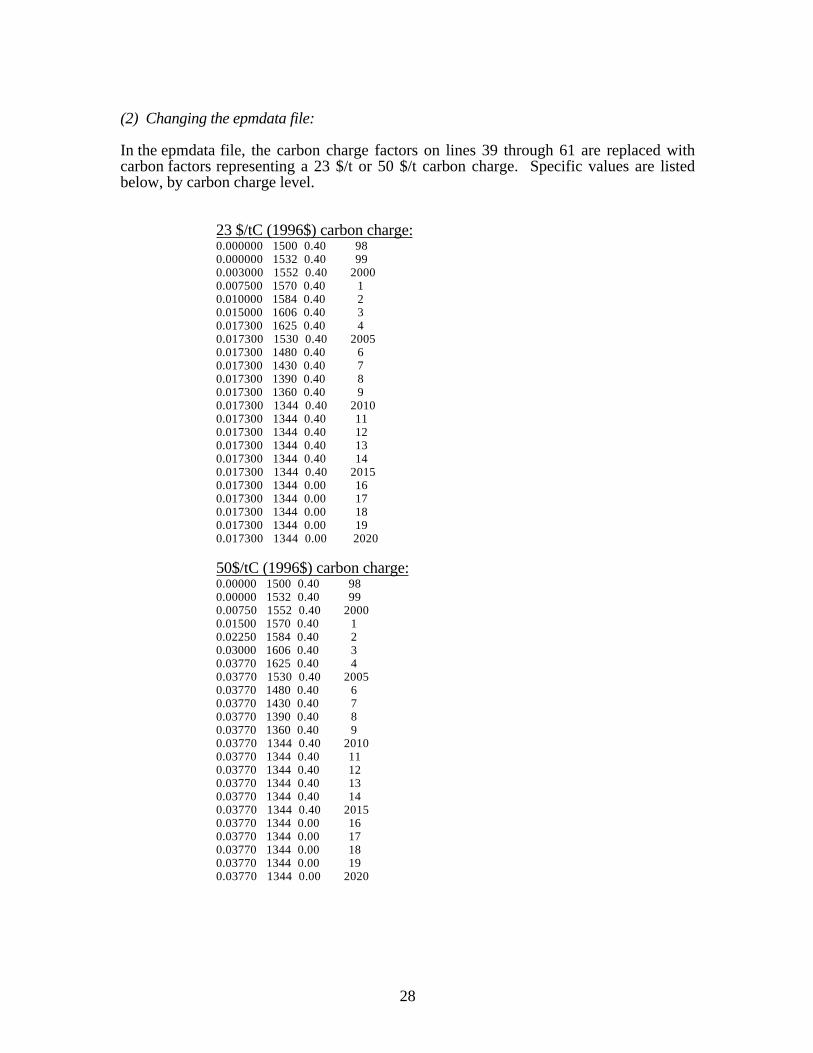
(2) Changing the epmdata file:

In the epmdata file, the carbon charge factors on lines 39 through 61 are replaced withcarbon factors representing a 23 $/t or 50 $/t carbon charge. Specific values are listedbelow, by carbon charge level.

23 $/tC (1996$) carbon charge:0.000000 1500 0.40 980.000000 1532 0.40 990.003000 1552 0.40 20000.007500 1570 0.40 10.010000 1584 0.40 20.015000 1606 0.40 30.017300 1625 0.40 40.017300 1530 0.40 20050.017300 1480 0.40 60.017300 1430 0.40 70.017300 1390 0.40 80.017300 1360 0.40 90.017300 1344 0.40 20100.017300 1344 0.40 110.017300 1344 0.40 120.017300 1344 0.40 130.017300 1344 0.40 140.017300 1344 0.40 20150.017300 1344 0.00 160.017300 1344 0.00 170.017300 1344 0.00 180.017300 1344 0.00 190.017300 1344 0.00 2020

50$/tC (1996$) carbon charge:0.00000 1500 0.40 980.00000 1532 0.40 990.00750 1552 0.40 20000.01500 1570 0.40 10.02250 1584 0.40 20.03000 1606 0.40 30.03770 1625 0.40 40.03770 1530 0.40 20050.03770 1480 0.40 60.03770 1430 0.40 70.03770 1390 0.40 80.03770 1360 0.40 90.03770 1344 0.40 20100.03770 1344 0.40 110.03770 1344 0.40 120.03770 1344 0.40 130.03770 1344 0.40 140.03770 1344 0.40 20150.03770 1344 0.00 160.03770 1344 0.00 170.03770 1344 0.00 180.03770 1344 0.00 190.03770 1344 0.00 2020

28

A.2 Electric utility sector

Early retirement of coal plants

In the LBNL-NEMS HELC case, coal capacity is retired through modifying the “retirementyear” field of the plant data file (pltf860.v1.68). These plants are retired over the years2000 to 2008.

Plants are selected among existing coal plants that are not retired by NEMS in the AEO98Reference Case. The online year for a plant is used as the criteria to select plants to beretired. The online year criteria for three levels of coal plant retirements are shown below:

Table A.2.1 Coal plant retirement level criteriaRetirement Level (GW) Retirement Criteria (1)

16 All coal plants online before 1955



(1) Plants retired by NEMS during the AEO98 Reference Case forecast period are not eligible for retirement

Early retirement of gas/oil steam turbine plants

A large portion of gas and oil steam turbine capacity is retired by NEMS in the baselineAEO forecast. In the LBNL-NEMS HELC case, all the remaining capacity for thistechnology (≈100GW) is retired over the years 2000 to 2008 through modifying the“retirement year” field for these plants in the plant data file (pltf860.v1.68).

Biomass co-firing

In section 7.3.1.1 of the Five Lab Study, the potential for biomass co-firing capacity isestimated to be between 8 and 12 GW by the year 2010. Using 10 GW of capacity as amidpoint, 10 GW of coal capacity is “converted” to biomass co-firing in regions of the USthought to have the greatest potential for this type of activity (the northeast and southeast).Since NEMS currently has no ability to handle biomass co-firing as a separate technology,modifications to simulate the adoption of biomass co-firing have been made to the plantdata file. This involves the gradual reduction of coal capacity through retirements coupledwith the addition of new biomass capacity. Individual coal plants chosen to have biomassco-firing are picked so that they do not fall within the retirement criteria for coal plantretirements (see above.)

The conversion of coal capacity to biomass capacity is achieved by first separating the coalcapacity to be retired through creation of an additional unit at a plant with a capacitycorresponding to the retirement amount. This unit is then given a retirement year between2000 and 2008, and remaining units at the plant have their capacities reduced by theretirement amount. Finally, new biomass capacity is added to the plant with an on-line yearcorresponding to the retirement year of the retired coal unit.

29

Increasing hydropower capacity

Section 7.3.1.3 of the Five Lab Study estimates that given relicensing issues andenvironmental regulations, the net capacity addition due to efficiency improvements andadded capacity will be between 10 GW and 16 GW. Taking 13 GW as a midpoint, newcapacity in existing hydropower plants is phased in over the years 2000 to 2008 in the plantdata file through additional units added to existing hydropower plants. This additionalhydropower capacity is distributed evenly across all 13 NERC regions.

Extending wind credit

In the ecpdat file, the last year of eligibility for the generation subsidy (UPIGSYL) forwind is changed from 1999 to 2020 and the generation subsidy duration (in years)(UPIGSYR) is changed from 10 to 25.

30

A.3 Residential sector

Energy efficiency

In the Five Lab Study HELC Case, increased energy efficiency reduces energyconsumption in 2010 by amounts shown in Table A.3.1.

Table A.3.1 Five Lab Study residential sector energy efficiency site energysavings (Quadrillion Btu)

Electricity Natural Gas Distillate LPGFive Lab Study HELC Case -0.77 -0.13 -0.03 -0.02

The following changes are made to the AEO98 Reference Case version of the NEMSresidential model to implement energy savings comparable to the Five Lab Study energysavings: implicit discount rates (Beta1/Beta2) are changed to 15% for all technologies afterthe year 1999 in the rtekty.v1.61 input data file, lighting efficiencies and market shares aremodified in the resd.f source code, and the growth in "Other" electricity consumption islimited in the resd.f source code. Detailed descriptions of these changes are listed below:

(1) Implicit discount rates are changed to 15% for all technologies after the year 1999 inthe rtekty.v1.61 data file

For each technology in the rtekty.v1.61 input file the following changes are made:

the line containing the technology characteristics for the year 2000 is duplicated

the lastyear field of the original line is set to 1999

the firstyear field of the duplicate line is set to 2000

the Beta1 field is changed so that the implicit discount rate (Beta1/Beta2) equals 0.15for all lines with firstyear fields greater than 1999

31

(2) Lighting efficiency and market share changes in the resd.f source code

Line 10043 is changed fromEFF(3)=88.00 ! SHOULD BE 88.00

to:EFF(3)=20.90 ! LBNL ! SHOULD BE 88.00

Lines 10047 through 10055 are changed from the following values:

LTMSHR(15,1)=0.93LTMSHR(15,2)=0.07LTMSHR(15,3)=0.00LTMSHR(26,1)=0.90LTMSHR(26,2)=0.10LTMSHR(26,3)=0.00LTMSHR(31,1)=0.88LTMSHR(31,2)=0.12LTMSHR(31,3)=0.00

to the following values:

LTMSHR(15,1)=0.70LTMSHR(15,2)=0.10LTMSHR(15,3)=0.20LTMSHR(26,1)=0.20LTMSHR(26,2)=0.20LTMSHR(26,3)=0.60LTMSHR(31,1)=0.20LTMSHR(31,2)=0.20LTMSHR(31,3)=0.60

32

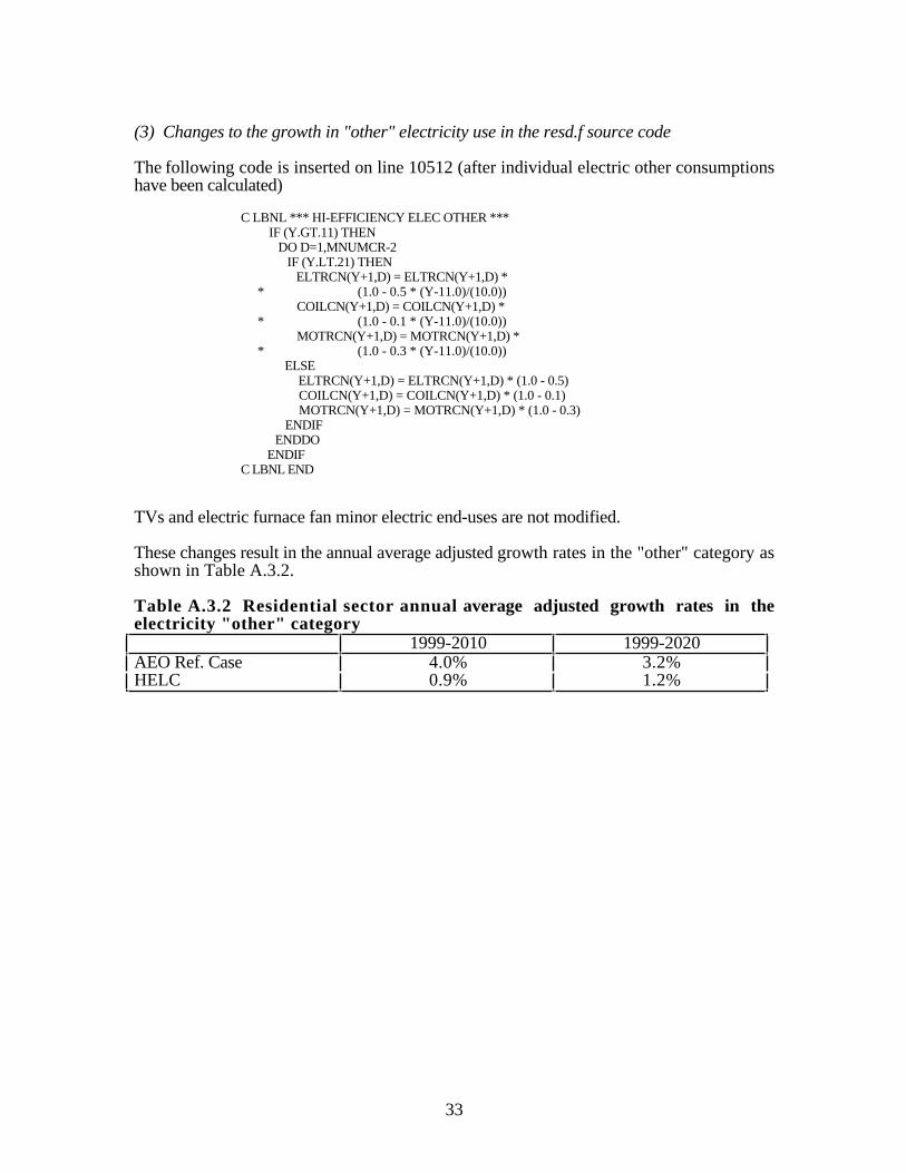
(3) Changes to the growth in "other" electricity use in the resd.f source code

The following code is inserted on line 10512 (after individual electric other consumptionshave been calculated)

C LBNL *** HI-EFFICIENCY ELEC OTHER *** IF (Y.GT.11) THEN DO D=1,MNUMCR-2 IF (Y.LT.21) THEN ELTRCN(Y+1,D) = ELTRCN(Y+1,D) * * (1.0 - 0.5 * (Y-11.0)/(10.0)) COILCN(Y+1,D) = COILCN(Y+1,D) * * (1.0 - 0.1 * (Y-11.0)/(10.0)) MOTRCN(Y+1,D) = MOTRCN(Y+1,D) * * (1.0 - 0.3 * (Y-11.0)/(10.0)) ELSE ELTRCN(Y+1,D) = ELTRCN(Y+1,D) * (1.0 - 0.5) COILCN(Y+1,D) = COILCN(Y+1,D) * (1.0 - 0.1) MOTRCN(Y+1,D) = MOTRCN(Y+1,D) * (1.0 - 0.3) ENDIF ENDDO ENDIFC LBNL END

TVs and electric furnace fan minor electric end-uses are not modified.

These changes result in the annual average adjusted growth rates in the "other" category asshown in Table A.3.2.

Table A.3.2 Residential sector annual average adjusted growth rates in theelectricity "other" category

1999-2010 1999-2020AEO Ref. Case 4.0% 3.2%HELC 0.9% 1.2%

33

A.4 Commercial sector

Energy efficiency

In the Five Lab Study HELC Case, increased energy efficiency reduces energyconsumption in 2010 by amounts shown in Table A.4.1.

Table A.4.1 Five Lab Study commercial sector energy efficiency siteenergy savings (Quadrillion Btu)

Electricity Natural Gas DistillateFive Lab Study HELC Case -0.59 -0.34 -0.03

The following three changes are made to the AEO98 Reference Case version of the NEMScommercial model to implement energy savings comparable to the energy savings in theFive Lab Study: implicit discount rates used in evaluating purchase decisions are changedto 14% plus the 10 year government bond interest rate for all end-uses in the years after1999 (which results in about an 18% discount rate in total), behavior rule constraints onnew equipment purchases for space heating and space cooling are relaxed after the year1999, and growth in the penetration of "Other" electricity use is limited. Detaileddescriptions of these changes are listed below:

(1) Discount rate changes in the kprem.v1.10 input data file

The distribution of time preference premiums is modified for all end-uses in all years after1999. The share of consumers using the 0.136 discount rate is set to 1.0 and all othercategories (10, 1.529, 0.554, 0.309, and 0.199) are set to 0.0. Note that the effectivediscount rate used in the commercial module is the discount rate in the kprem.v1.10 inputfile plus the 10 year government bond interest rate (3.7% to 4.0% real interest rate.)

(2) Changes to behavior rules in the kbehav.v1.11 and the comm.f source code

The kbehav.v1.11 file is duplicated and renamed "kbehav_sf." In the kbehav_sf file, forspace cooling and space heating new purchase decisions, all shares allocated to the "sametechnology" behavior rule are moved to the "same fuel" behavior rule.

The behavior rules in the kbehav_sf input file are then used for forecast years after 1999 bymaking the following change in the comm.f source code:

Line 3295 is changed from

IF (CURIYR.EQ.CMFirstYr .AND. CURITR.EQ.1) THEN

to IF ((CURIYR.EQ.CMFirstYr .AND. CURITR.EQ.1) .OR. ! LBNL * (CURIYR.EQ.11 .AND. CURITR.EQ.1)) THEN ! LBNL

and after Line 3318, the following code is added

IF (CURIYR.EQ.11) THEN ! LBNL WRITE(*,*) 'YEAR 2000 CHANGING KBEHAV FILE' ! LBNL OPEN(INFILE,file='input/kbehav_sf',STATUS='old')! LBNL ENDIF

34

(3) Changes to the growth in "other" electricity use in koffpen.v1.9 input data file and thecommercial source code

In the koffpen.v1.9 file, the annual market penetration index for “other" end-uses is set to85% of its default value. This 15% reduction is phased in linearly from 2000 to 2009 andis then constant from 2010 to 2020.

In the commercial source code (comm.f), the following code is inserted on line 7303 todecrease the non-building electricity energy use (a component of the electricity ‘other’) by15%. This reduction is phased in linearly from 2000-2009 and held constant from 2010 to2020.

C RCR LBNL decrement non-bldg energy use by 20% IF (CURIYR.GT.11) THEN DO r= 1, MNUMCR-2 IF (CURIYR.LT.21) THEN CMNonBldgUse(1,r,CURIYR) = CMNonBldgUse(1,r,CURIYR) * * (1.0 - 0.15 * (CURIYR-11.0)/(10.0)) ELSE CMNonBldgUse(1,r,CURIYR) = CMNonBldgUse(1,r,CURIYR) * * (1.0 - 0.15) END IF END DO END IFC RCR LBNL END

These changes result in the annual average adjusted growth rates in the "other" category asshown in Table A.4.2.

Table A.4.2 Commercial sector annual average adjusted growth rates in theelectricity "other" category

1999-2010 1999-2020AEO Ref. Case 3.1% 2.5%HELC 1.6% 1.7%

35

A.5 Industrial sector

Energy efficiency

Energy efficiency savings estimated using the LIEF model (rather than Five Lab Studysavings) are implemented in the industrial module; see Table A.5.4 for energy savings byindustrial sub-sector.

The changes made to the industrial model represent modifications to the EIA Hi-Tech Case.The following parameters are changed: the variable RETRATE is modified by sub-sectorfor all sub sectors, the HITECH modifier to the ENPINT variable is modified by sub-sector and fuel type for sub-sectors 1-6 and 14-15, and the TPC coefficients are varied bysub-sector and fuel type for sub-sectors 7-13. These LBNL High Efficiency Caseparameters are chosen so that energy savings are within +/- 5% of the LIEF energyefficiency savings (See Table A.5.4.) These changes are summarized below.

(1) Changing the RETRATE coefficients

On line 4511, the source code is expanded so that different RETRATES can be used foreach of the industrial sub-sectors. See Table A.5.1 below for values used in the EIAAEO98 HI-Tech Case and the LBNL-NEMS HELC Case.

Table A.5.1 Retirement rates in the EIA AEO98 Hi-Tech case and LBNL-HEMS HELC case

Industrial Sub-Sector RETRATE Value

EIA AEO98 Hi-Tech Case LBNL-NEMS HELC Case

1 Agriculture-Crops 2.0 2.0

2 Agriculture-Other 2.0 2.0

3 Coal Mining 2.0 2.0

4 Oil/Gas Mining 2.0 2.0

5 Metal/Other Mining 2.0 2.0

6 Construction 2.0 2.0

7 Food 2.0 4.0

8 Paper 2.0 2.5

9 Bulk Chemicals 2.0 2.2

10 Glass 2.0 2.0

11 Cement 2.0 2.0

12 Steel 2.0 2.0

13 Aluminum 2.0 3.5

14 Metals Durables 2.0 2.0

15 Other 2.0 2.0

36

(2) Changing the HITECH modifiers to the ENPINT variable

In six locations in the ind.f source code (lines 5333, 5464, 6029, 6202, 6628, and 6993),the HITECH IF Statement is expanded so that varying modifiers can be used for theindustrial sub-sectors 1 through 6. See Table A.5.2 below for values used in the EIAAEO98 Hi-Tech Case and the LBNL-NEMS HELC Case.

Table A.5.2 ENPINT modifiers in the EIA AEO98 Hi-Tech case andLBNL-NEMS HELC case

Industrial Sub-Sector ENPINT Modifier


Fuels Elec Fuels Elec

1 Agriculture-Crops -0.0682 -0.0682 -0.190 -0.190

2 Agriculture-Other -0.0682 -0.0682 -0.200 -0.200

3 Coal Mining -0.0682 -0.0682 -0.170 -0.170

4 Oil/Gas Mining -0.0682 -0.0682 -0.200 -0.200

5 Metal/Other Mining -0.0682 -0.0682 -0.220 -0.220

6 Construction -0.0682 -0.0682 -0.001 -0.150

14 Metals Durables -0.0682 -0.0682 -0.130 -0.130

15 Other -0.0682 -0.682 -0.200 -0.260

(3) Changing the TPC coefficients

On line 5640, the source code is expanded so that different TPC sensitivities can be usedfor electricity and non-electricity processes for each of the industrial sub-sectors. See TableA.5.3 for values used in the EIA AEO98 Hi-Tech Case and the LBNL-NEMS HELC Case.

Table A.5.3 TPC parameters in the EIA AEO98 Hi-Tech case and LBNL-NEMS HELC case

Industrial Sub-Sector TPC Parameter


Fuels Elec Fuels Elec

7 Food 2.0 2.0 4.0 4.0

8 Paper 2.0 2.0 1.8 2.2

9 Bulk Chemicals 2.0 2.0 1.2 3.0

10 Glass 2.0 2.0 1.7 1.5

11 Cement 2.0 2.0 1.7 1.9

12 Steel 2.0 2.0 4.0 1.1

13 Aluminum 2.0 2.0 4.0 3.5

37

The following table summarizes the energy efficiency savings estimated using the LIEFmodel and the corresponding savings implemented in the LBNL-NEMS model.

Table A.5.4 Energy efficiency savings predicted by the LIEF model andimplemented in the LBNL-NEMS High Efficiency case

Industrial Sub-Sector LIEF LBNL-NEMS

Estimated EnergySavings

Percentage(%)

Energy Savingsrelative to

NEMS BaselineEnergy Use

(TBtu)

High Efficiency CaseEnergy Savings (1)

(TBtu)

Site Electricity

1 Agriculture-Crops 16% -15 -15

2 Agriculture-Other 16% -6 -6

3 Coal Mining 16% -9 -9

4 Oil/Gas Mining 16% -24 -24

5 Metal/Other Mining 16% -21 -19

6 Construction 16% -16 -16

7 Food 24% -37 -25

8 Paper 12% -26 -26

9 Bulk Chemicals 12% -33 -32

10 Glass 8% -4 -4

11 Cement 8% -3 -3

12 Steel 4% -7 -7

13 Aluminum 12% -29 -29

14 Metals Durables 16% -86 -90

15 Other 24% -172 -164

Total - -488 -469

Fuels1 Agriculture-Crops 16% -92 -89

2 Agriculture-Other 16% -37 -36

3 Coal Mining 16% -21 -20

4 Oil/Gas Mining 16% -195 -194

5 Metal/Other Mining 16% -60 -57

6 Construction 16% -264 -328

7 Food 16% -133 -119

8 Paper 12% -286 -278

9 Bulk Chemicals 12% -606 -740

10 Glass 8% -19 -20

11 Cement 8% -26 -26

12 Steel 8% -159 -120

13 Aluminum 12% -4 -4

14 Metals Durables 16% -129 -122

15 Other 16% -280 -270

Total - -2311 -2423

(1) High Efficiency savings are reported (rather than HELC) to exclude feedback from supply-side options.

38

Increase natural gas cogeneration

Based on off-line analysis (US DOE 1997b), natural gas cogeneration is increased by 35GW (@ 70% electric capacity factor), or 215 TWh by 2010. The following changes aremade to the ind.f source code to implement this increase: natural gas cogeneration isincreased 215 TWh by 2010 in the ELGEN calculation, the associated gas fuelconsumption is removed from the GCTFUEL calculation, and the gas fuel consumption isaccounted for in the FUELADD calculation using a net heat rate of 1.75.

(1) Increasing natural gas cogeneration in the ind.f source code

Lines 7834-7838 which contain the following code: IF(TEMP(11).GT.0.0.and.cinter(inddir,indreg,pm).ne.0.0)THEN ELGEN(pm)=(EXP(cINTER(inddir,indreg,pm)))*(STEMCUR**GSTEAM) ELSE ELGEN(pm)=0.0 ENDIF

are replaced by the following code

C ***** LBNL --- INCREASING GAS COGEN BY 215 TWh -- 35GW @ 70%CF IF (PM.EQ.2) THENC OPEN(1,FILE='cogendump',STATUS='old')C WRITE(1,*)'YR is ',IYR,'--BASELINE COGEN IS ',ELGEN(2) IF ((IYR.GE.2001) .AND. (IYR.LT.2010)) THEN ELGEN(pm) = ELGEN(pm) * (IYR-1999.0) / 10.0 * 6.0 ELSE IF (IYR.GE.2010) THEN ELGEN(pm) = ELGEN(pm) * 6.0 ENDIFC WRITE(1,*)' --MODIFIED COGEN IS ',ELGEN(2)C CLOSE(1) ENDIFC ***** LBNL END *****

(2) Removing incremental gas cogeneration from GCTFUEL calculation

After Line 8210, which contains the following code:

GCTFUEL=ELGEN(2)*GENEQPHTRT(2)/3412.0 ! Trillion Btu

the following code is inserted:

C ***** LBNL ***** REMOVING INCREMENTAL GAS COGENERATION FROM GCTFUEL IF ((IYR.GE.2001) .AND. (IYR.LT.2010)) THEN GCTFUEL=GCTFUEL / (6.0 * (IYR - 1999.0) / 10 ) GCTFUEL=GCTFUEL + * ELGEN(2) * 5.0/6.0 * (IYR - 1999.0) / 10 * 1.75 ELSE IF (IYR.GE.2010) THEN GCTFUEL=GCTFUEL / 6.0 GCTFUEL=GCTFUEL + * ELGEN(2) * 5.0/6.0 * 1.75 ! 1.75 HEAT RATE 4 INC. GAS ENDIFC ***** LBNL END *****

39

(3) Accounting for incremental gas cogeneration

Lines 8313 to 8321, which contain the following code:

DO I = L,M ! division aggregated to region DO IP = 1,3 ! prime mover DO IF = 1,6 ! fuel fueladd(INDREG,if) = fueladd(indreg,if) + 0.5 * 1 (SICGEN(I,YR,INDDIR,IF,IP,3)*3412.0/10**6) ENDDO ENDDO ENDDO

are replaced by the following code:

DO I = L,M ! division aggregated to region DO IP = 1,3 ! prime mover DO IF = 1,6 ! fuel fueladd(INDREG,if) = fueladd(indreg,if) + 0.5 * 1 (SICGEN(I,YR,INDDIR,IF,IP,3)*3412.0/10**6)!C ***** LBNL --- ACCOUNTING FOR GAS COGEN WITH HEATRATE OF 1.75 IF ((IYR.GE.2001) .AND. (IYR.LT.2010)) THEN fueladd(INDREG,if) = fueladd(INDREG,if) - * 0.5 * 5.0/6.0 * (IYR - 1999.0) / 10 * * (SICGEN(I,YR,INDDIR,IF,IP,3)*3412.0/10**6) ELSE IF (IYR.GE.2010) THEN fueladd(INDREG,if) = fueladd(INDREG,if) - * 0.5 * 5.0/6.0 * * (SICGEN(I,YR,INDDIR,IF,IP,3)*3412.0/10**6) ENDIFC ***** LBNL END ***** ENDDO ENDDO ENDDO

40

A.6 Transportation sector

Energy efficiency

The LBNL-NEMS HELC transportation sector assumptions are a replication of the FiveLab Study HELC Case assumptions. The Five Lab Study transportation sector analysisused the AEO97 Version of NEMS. We modified the Five Lab Study input files to accountfor structural changes in the NEMS model from the AEO97 Version to the AEO98 Version,but otherwise assumptions are consistent between the Five Lab Study HELC Case and theLBNL-NEMS HELC Case.

The LBNL-NEMS HELC Case makes changes to the horsepower vs. efficiency trade-offin the tran.f source code, the technology and behavior characteristics in the cffuel.v1.3input file, and technology and behavior characteristics in the trninput input file. Thesechanges are described below:

(1) Changing the horsepower vs. efficiency trade-off in the tran.f source code

The equation on line 1517 of the NEMS tran.f source code shown below

ADJHP(ICL,IGP,IFT)=PERFFACT(ICL,IGP)*4.0* & (((INCOME(YEAR)/INCOME(YEAR-1))**0.9* & (PRICE(ICL,IGP,YEAR-1,IFT)/PRICE(ICL,IGP,YEAR,IFT))**0.9* & (FE(ICL,IGP,YEAR,IFT)/FE(ICL,IGP,YEAR-1,IFT))**0.2* & (FUELCOST(YEAR-1)/FUELCOST(YEAR))**0.2) - 1.0)

is replaced with the following equation in the LBNL-NEMS tran.f source code:

ADJHP(ICL,IGP,IFT)=PERFFACT(ICL,IGP)*4.0* & (((INCOME(YEAR)/INCOME(YEAR-1))**0.5* & (PRICE(ICL,IGP,YEAR-1,IFT)/PRICE(ICL,IGP,YEAR,IFT))**0.5* & (FE(ICL,IGP,YEAR,IFT)/FE(ICL,IGP,YEAR-1,IFT))**0.1* & (FUELCOST(YEAR-1)/FUELCOST(YEAR))**0.1) - 1.0)

41

(2) Changing the truck technology characteristics in the cffuel.v1.3 input file:

There are no differences between the default AEO97 and default AEO98 versions of thecffuel.v1.3 file. Therefore, the original Five Lab Study HELC cffuel input file is used asthe LBNL-NEMS HELC Case cffuel input file. Table A.6.1 lists the technologyparameters that we modified in the cffuel input file. Table A.6.2 lists the technologieswhich we modified in the cffuel file, as well as which parameters (see Table A.6.1 forparameter number mapping) we modified for each technology in the medium and heavytruck categories.

Table A.6.1 Technology parameters we modified in the cffuel fileParameter Number Parameter Name Parameter Description

1 CAVAILYR year in which new technology becomes available2 FUELAPPL technology-fuel applicability matrix3 TRIGPRC technology trigger price4 CYCLE years until 99% penetration5 PRCVAR price variation coefficient6 ESHRT maximum share of technology at trigger price7 PRCVAR superseding matrix8 MPGINCR incremental technology fuel economy improvement

Table A.6.2 Technology parameters* we modified by technology in thecffuel file by truck category

Modified Technology Parameter Number*Truck Model Technologies medium trucks heavy trucks

Aerodynamic Features 3 3Radial Tires 3 3

Axle or Drive Ratio 3 3Fuel Economy Engine 3 3

Variable Fan Drive 3 3Improved Tires & Lubricants 3,4,8 3,4,6,8Electronic Engine Controls 3,4,8 3,4,6,8

Electronic Transmission Controls 3,4,8 3,4,6,8Advanced Drag Reduction 1,2,,4,5,6,8 1,3,4,5,6,8

Turbocompound Diesel Engine 1,2,3,4,5,6,8 1,3,4,6,8Heat EngineÄLE-55 1,2,4,5,6,8 1,3,4,5,6,8

Blank 14 1,2,3,4,5,6,7,8 1,2,3,4,5,6,7,8Blank 15 1,2,3,4,5,6,8 1,5,8

* See Table A.6.1 for parameter number mapping

42

(3) Changing the technology characteristics in the trninput.v1.42 input file:

The AEO98 Reference Case version of the trninput file is modified to mirror the Five LabStudy HELC version of the trninput file. When necessary, HELC trends are extendedfrom 2015 to 2020 in the AEO98 Version of the file (trninput.v1.42). Otherwise, changesare generally one for one.

The trninput file is a Lotus-123 file. We use Lotus 1 Release 5 for Windows NT to modifythe trninput file. In the NEMS model, the nemswk1.f source code is responsible forreading data from lotus (.wk1) binary files. Even though the modified trninput.v1.42 fileis saved in the appropriate older Lotus format, the nemswk1 source code is unable to readnine variables from the input file. The nine variables are C1T, C2T, C3T, C4T, COEF$A,COEF$B, COEF$C, T50, and T90. To fix this problem, these variables (none of whichare changed in the HELC case) are overwritten with their AEO98 Reference Case values inthe READWK1 subroutine in the tran.f source code.

Modifications to the trninput.v1.42 are described below. The purpose of thisdocumentation is to describe which variables in the input file are changed. We do notdocument the magnitude or direction of changes. For a complete comparison, downloadthe specific files from our ftp server (see beginning of Appendix A for instructions) and usethis documentation as a guide through the files.

In the documentation below, descriptions of changes are separated by transportationmodule, as they are characterized in the trninput file. Specific row numbers are used torefer to the relevant areas of the input file section. The row numbers correspond to theAEO98 version of the input file (trninput.v1.42).

Light Duty Vehicle Module (rows 1 to 1151)

Section 1 (rows 1 to 183)

In this section of the input data, there are seven technology parameters for the fifty sevendefault technologies. The technologies are separated by car and light truck categories.Table A.6.3 lists the seven fuel economy model technology parameters for eachtechnology. Table A.6.4 lists the technologies which are modified, as well as whichparameters (see Table A.6.3 for parameter number mapping) are modified for eachtechnology in the car and light truck category. Twenty one of the fifty six defaulttechnologies are modified and five new technologies are added in this section of the inputfile.

Table A.6.3 Technology parameters we modifiedParameterNumber

ParameterName

Parameter Description

1 TFET fractional change (%) in fuel economy2 TCABST change in cost ($)3 TCWGTT weight based change in cost ($/lb)4 TWABST change in weight (lbs)5 TWWGTT change in weight based on original weight (lb/lb)6 IFRSTT first year technology is available7 THPT fractional change (%) in horsepower

43

Table A.6.4 Technology parameters* we modified by technology by car andlight truck category

Technologies TECHIDT Modified Parameterscar light truck

Material Substitution III 4 - 6Material Substitution IV 5 6 6Material Substitution V 6 6 6

Drag Reduction IV 9 6 6Drag Reduction V 10 6 6

CVT 14 2 6Electronic Transmission II 17 - 6

8C/8V 24 - 6Engine Friction Reduction II 29 - 6Engine Friction Reduction III 30 6 6Engine Friction Reduction IV 31 6 6

VVT I 32 2 6VVT II 33 2,6 6DISC** 34 1,2,6 6

Two Stroke 35 6 6Tires II 43 1,6 2Tires III 44 1,6 1,6Tires IV 45 1,6 1,6ACC II 47 - 6

EPS 48 - 64WD Improvements 49 - 6

Drag Reduction VI*** 57 1,2,3,4,5,6,7 1,2,3,4,5,6,7Turbo Direct Injection Diesel*** 58 1,2,3,4,5,6,7 1,2,3,4,5,6,7

Hybrid Gasoline*** 59 1,2,3,4,5,6,7 1,2,3,4,5,6,7Hybrid Diesel*** 60 1,2,3,4,5,6,7 1,2,3,4,5,6,7

Gasoline Fuel Cell Hybrid*** 61 1,2,3,4,5,6,7 1,2,3,4,5,6,7* See Table A.6.3 for parameter number mapping** replaces lean burn technology in the AEO98 Reference Case*** technology added (rather than modified)

44

Section 2 (rows 231-567)

In this section of the Fuel Economy Model input data, base year and maximum marketshares for each of 61 (56 default + 5 new) technologies in seven size classes are listed.Table A.6.5 lists which size class is modified for each technology by marketshare type, andvehicle group.

Table A.6.5 Technology marketshares we modified by marketshare type,vehicle group, and size class

Tech ID Size Class Modifiedbaseyear marketshare maximum marketshare

vehicle group vehicle group1 2 3 4 1 2 3 4

front wheel drive 3 - - - 2 - - -drag reduction II 3 - - - 2 - - -

TCLV 3 - - - 2 - - -4-speed automatic 3 - - - 2 - - -

roller cam - - - - 2 - - -OHC 4 2 - - - 2 - - -4C/4V - - - - 2 - - -

engine friction reduction I - - - - 2 - - -air pump 3 - - - 2 - - -

DFS 3 - - - 2 - - -oil SW-30 3 - - - 2 - - -air bags 3 - - - 2 - - -

ABS 3 - - - 2 - - -Drag Reduction VI* 1-7 1-7 1-7 1-7 1-7 1-7 1-7 1-7

Turbo Direct Injection Diesel* 1-7 1-7 1-7 1-7 1-7 1-7 1-7 1-7Hybrid Gasoline* 1-7 1-7 1-7 1-7 1-7 1-7 1-7 1-7Hybrid Diesel* 1-7 1-7 1-7 1-7 1-7 1-7 1-7 1-7

Gasoline Fuel Cell Hybrid* 1-7 1-7 1-7 1-7 1-7 1-7 1-7 1-7* technology added (rather than modified)


On row 689, the payback period is changed and on row 690, the discount rate is changed.

Section 4( rows 857 to 1151)

There are no changes in this section of the input data.

45

Light Duty Vehicle Fleet Module -- (rows 1152 to 1236)


Light-Duty Vehicle Stock Module (rows 1237 o 1327)

Section 1 (rows 1237 to 1312 )

The degradation factors for cars and light trucks by year (CDG and LTDF) are modified inthis section of the data.



Freight Transport Module (rows 1407 to 1432)

Section 1 (no longer in trninput file)

The changes to TBETA1 and TBETA2 in the Five Lab Study trninput file are not recreatedin the LBNL-NEMS HELC trninput file because this section of the input data is removedfrom the AEO98 Version of the trninput file (possibly replaced by the Commercial LightTruck Module).

Section 2 (rows (1421 to 1425)

In this section of the input data, the freight rail efficiency by year (FERAIL) is modified.

Section 3 (1426 to 1432)

In this section of the input data, the freight ship efficiency by year (FESHIP) is modified.

Air Travel Module (rows 1433 to 1463)

In this section of the input data, there are several modifications. The load factor time-seriesdata for domestic and international travel are increased (LFDOM and LFINT). The startingyear (TRIGYEAR), cost (TRIGCOST), and incremental efficiency (EFFIMP)improvement parameters for the six generic air travel efficiency technologies are modified.Also, the "rho" times-series data for narrow and wide-body aircraft (RHON and RHOW)are modified.

Miscellaneous Transportation Energy Demand Module (rows 1464 to 1549)


46

APPENDIX B: COMPLETE LIST OF LBNL-NEMS HIGH-EFFICIENCY/LOW CARBON CASES1 AEO98 Reference Case2 23 $/t Carbon Charge Case3 50 $/t Carbon Charge Case4 High Efficiency Case5 16GW Coal and 0GW Gas-Oil Retirements Case (16/0)6 42GW Coal and 0GW Gas-Oil Retirements Case (42/0)7 63GW Coal and 0GW Gas-Oil Retirements Case (63/0)8 0GW Coal and 100GW Gas-Oil Retirements Case (0/100)9 16GW Coal and 100GW Gas-Oil Retirements Case (16/100)10 42GW Coal and 100GW Gas-Oil Retirements Case (42/100)11 63GW Coal and 100GW Gas-Oil Retirements Case (63/100)12 Biomass Cofire Case13 Industrial Cogen Case14 Hydro Refurbishment Case15 Wind Tax Credit Extension Case16 Supply Side (cofire/cogen/hydro/wind) Case

17 23 $/t Carbon Charge/High Efficiency Case18 23 $/t Carbon Charge 16GW Coal and 100GW Gas-Oil Retirements Case19 High Efficiency 16GW Coal and 100GW Gas-Oil Retirements Case

20 HELC Case 23$/tC (0/0)--includes High Efficiency (4) and Supply Side options (16)21 HELC Case 23$/tC (16/0)--includes High Efficiency (4) and Supply Side options (16)22 HELC Case 23$/tC (42/0)--includes High Efficiency (4) and Supply Side options (16)23 HELC Case 23$/tC (63/0)--includes High Efficiency (4) and Supply Side options (16)24 HELC Case 23$/tC (0/100)--includes High Efficiency (4) and Supply Side options (16)25 HELC Case 23$/tC (16/100)--includes High Efficiency (4) and Supply Side options (16)26 HELC Case 23$/tC (42/100)--includes High Efficiency (4) and Supply Side options (16)27 HELC Case 23$/tC (63/100)--includes High Efficiency (4) and Supply Side options (16)



47

APPENDIX C: SUMMARIES OF KEY REVIEW COMMENTS

As described in the preface, this report underwent extensive technical review. Weparaphrase the key substantive comments received below, with our responses. We do notinclude the myriad comments that noted the many places where the initial draft was unclearor inconsistent, because those are not of general interest. We are grateful to the reviewersfor all their comments, since they resulted in a vastly improved report.

Comment (1): The paper assumes that the reader is familiar with the NEMS model. Wewould certainly suggest at least a brief description (and perhaps a flowchart) of how themodel works.

Response: In helping our readers better understand the context of our integratedscenario analysis, we expanded the discussion about the NEMS model, including adiagram to illustrate its key components and interactions. In addition, we havegiven readers more of a context to explain the background of the Five-Lab studythat drives many of our scenario assumptions.

Comment (2): The policy relevance of this study is high, perhaps higher than isacknowledged in the introductory discussion. The EU (and most developing countries) isvery concerned that the U.S. will attempt to fulfill most of its Kyoto obligation byacquiring carbon allowances from abroad. To prevent this strategy, which the EU regardsas contrary to the intent of the Protocol, the EU along with several LDC's inserted intoArticle 17 the provision that emissions trading “shall be supplemental to domestic actions.”

Response: Although we are not in a position to evaluate this statement, we notethat the results of our scenario analysis strongly suggest the U.S. economy willbenefit from increased domestic technology investments.

Comment (3): We do not believe the Five-Lab energy efficiency potentials are realistic.

Response: Our focus was on creating scenarios that illustrate the economic andenvironmental opportunities associated with a high-efficiency/low-carbontechnology path. Although the American Petroleum Institute and others havewritten commentaries that are critical of the Five-Lab findings, the resourcepotential for this path is well documented in a large number of other studies that wereference. Whether one believes these potentials or not, our goal was to learn whatwe could about such technology-based scenarios using the LBNL-NEMSintegrating framework.

The authors believe that a combination of an emissions trading program and avariety of different non-price policies can lead to changes in energy service marketsof the magnitude required. These non-price policies include voluntary agreementswith industry, cost-effective minimum efficiency standards, ENERGY STARprograms, utility incentive programs funded through “line charges,” targeted taxcredits, golden carrots, government and industry purchases of high efficiencytechnologies now on the market, and technology procurement by government andindustry for technologies close to commercialization. The program experience over

49

the last two decades solidly demonstrates that these non-price programs work welland have been shown to be cost-effective.

Comment (4): If indeed the economy could costlessly achieve the energy savings posited itwould be beneficial. But the savings are not costless. Aside from the fact that a $23/tcarbon charge is needed, many would see large additional costs, explicit and hidden, in theregime being analyzed. These costs must be taken into account in assessing the overalleconomic impact.

Response: This is an important point. As a significant improvement in our finalstudy, we have included a more detailed estimate of the investment, transaction andprogram costs necessary to drive the kind of scenarios illustrated in this analysis.Tables 3a and 3b summarize our findings that a high-efficiency/low-carbon pathcan lead to a net economic benefit for the U.S. economy. We recognize, however,that more work needs to be done in this area.

Comment (5): The criticism of price-driven studies here is overdone and unwarranted.

Response: We agree, and to that extent we have modified the discussion in thatregard. We note, however, the significant evidence suggesting that a “smart” set ofpolicies and programs can reduce the size of the price signal that might otherwise beneeded to ease the economy onto a cost-effective technology path of reducinggreenhouse gas emissions. Price matters, but it is not all that matters. Among therequirements are that the signal be clear and unambiguous, not necessarily large.Again, this assumes effective policies and programs such as those described incomment (3) above.

Comment (6): It is important to explicitly lay out the exact “non-price” policies that areneeded to achieve the level of energy efficiency levels in the Five-Lab scenario.

Response: We agree that this is an important step, but it was not possible to do sowithin the strict time and resource constraints of this study. We have added text todescribe “the programs-based approach” and listed some of the non-price policiesthat would be important in any large-scale effort to implement energy efficiency.We have also explicitly accounted for program costs in our summary cost-benefitanalysis, just as the Five-Lab study did.

Comment (7): The report is too critical of the NEMS modeling framework

Response: The statements about the limitations of the NEMS modeling frameworkare important because NEMS is the official model of the US DOE, and it isimportant for the policy analysis community to understand its limitations. Thisshould in no way be taken to imply that we disapprove of the NEMS framework.In fact, we believe it is the best of the integrated models, because of itscomprehensive treatment of supply-side technologies (particularly in the electricitysector) and its detailed treatment of energy demand at the end-use level. As one of

50

the few users of NEMS outside of EIA, we believe it is our responsibility to beexplicit in whatever technical concerns we have about the model, because few otherpeople are in a position to do so. EIA continually makes improvements in theirmodeling framework every year, in part as a response to improved data andanalyses from researchers outside EIA. We believe that explicitly listing areaswhere the model can be improved is helpful for all who are concerned withimproving the modeling of U.S. energy policies.

Comment (8): The AEO forecast embodies historical relationships with little change frompast trends, but you are clearly moving away from that historical record in a positive way,and that needs to be brought out in your analysis.

Response: This is also an important issue, both within the modeling and the policyarenas. We think the evidence points in the direction of establishing a smart set ofpolicies and programs that can break with historical relationships. This isespecially true with respect to implementing a high-efficiency/low-carbon future.We also believe that the historical record has not been fully understood with respectto the ongoing opportunities to close that efficiency gap. The current generation ofEnergy Star programs and the various Research and Development initiativessupported by the U.S. Department of Energy all underscore this point.

Comment (9): Why switch in mid-stream to referencing the AMIGA model? What is thepedigree of this model, and what confidence can we place in its conclusions?

Response: Our previous reference to the results found in our AMIGA analysis wasunclear. We have attempted to strengthen that discussion. AMIGA shows thatmodel structure matters with respect to anticipated scenario outcomes. We cite theAMIGA analysis to underscore that a combination of policies and price signals canactually accomplish the twin objectives of reducing carbon emissions andmaintaining economic activity. As noted in both the reference to AMIGA, and theaccompanying footnote, it is a CGE model developed by the Argonne NationalLaboratory. The model has a substantial documentation that we can provide uponrequest.

Comment (10): Cost effectiveness of retirements and repowering should be investigated ona regional basis.

Response: This is an excellent point that we didn't have time to explore. We notedthat regional fuel prices should be a key area of investigation in the Future Worksection.

51

Comment (11): Many carbon savings options, such as repowering of coal-fired powerplants with natural gas, renewables, and advanced efficiency technologies, are not includedin the scenarios.

Response: We added a few paragraphs in the Future Work section to describe theones we feel are missing or need more exploration. We will investigate these in ourlater work.

Comment (12): It is interesting that your HELC case has declining prices and decliningdemand. This result seems counterintuitive from the perspective of Economics 101.

Response: It is important to understand that the non-price policies posited in ourscenarios reduce the barriers to the adoption of efficiency technologies (thesetechnologies are cost effective from society's perspective). These policies are notdependent on energy prices for their effectiveness, and hence can reduce demandfor energy use. This reduction in demand will then put downward pressure onprices. There will be some "takeback" due to this decline in prices. As a result,some households and businesses may take back some of the energy savings in theform of increased comfort and slightly higher energy use. However, the empiricalresearch on this topic shows this effect to be small.

The decline in energy prices from implementing these non-price policies is a majorbenefit to society that is not typically counted in bottom-up analyses of the costs ofreducing carbon emissions.

Comment (13): The HELC case involves diverting capital from other uses, so that there isan opportunity cost to these investments that is not included in your analysis

Response: The HELC case displaces capital intensive supply-side investments withcheaper demand-side investments, and it therefore results in less use of capital. Ifanything, this opportunity cost argument cuts in the opposite direction from the onethe commenter intended.

Comment (14): Strengthen the comments on macro effects found in the LBNL-NEMS.That's a weak point in the model so you should be clear on that yourselves.

Response: We agree with this point. Since the AEO98 version of NEMS does nottrack either energy efficiency technology investments or energy bill savings withrespect to their impact on GDP and personal consumption expenditures, the modelmay understate the positive impacts of a cost-effective technology path. It is forthat reason that we expanded the discussion on the full investment and programtransition costs to establish the net positive benefits of scenarios bolstered by theFive-Lab study and similar analysis.

52

APPENDIX D: KEY OUTPUTS FROM SELECTED MODELING RUNS

The following tables summarize key results from our runs. Each column represents ascenario that combines demand-side and supply side options in different ways. The firsttwo pages show results in 2010, and the second two show results in 2020. The last tableshows fuel use by fuel type and sector for selected scenarios in 2010 and 2020.

53

Table D-1: LBNL-NEMS High-Efficiency/Low Carbon Cases All-Sector Forecast Summary 2010 Page 1 of 2

AEO98 LBNL-NEMS LBNL-NEMS LBNL-NEMS LBNL-NEMS LBNL-NEMSRef 23 $/t C-C High-Eff Coal Retire Gas-Oil Retire SupplySide

Case Case Case Case Case Casedemand side efficiency measures - - hieff - - -

carbon charge ($/tC) - 23 - - - -coal retirements (GW) - - - 16 - -

natural gas and oil retirements (GW) - - - - 100 -supply-side improvements - - - - - cf/cg/hy/wd

2010 2010 2010 2010 2010 2010

Primary Energy (Quadrillion Btu)Residential 21.6 21.2 20.6 21.5 21.5 21.6Commercial 16.9 16.6 15.4 16.8 16.8 16.9Industrial 40.5 40.2 36.6 40.4 40.1 39.5Transportation 33.1 32.8 29.7 33.1 33.1 33.1Total 112.2 110.8 102.3 111.7 111.4 111.2

Electricity Sales (TWh)Residential 1350 1338 1201 1349 1349 1352Commercial 1200 1186 1041 1199 1200 1205Industrial 1282 1314 1106 1283 1267 1143Transportation 46 46 53 46 46 46Total 3877 3883 3400 3877 3861 3746

Carbon Emissions by Sector (Mt)Residential 338 327 314 333 337 332Commercial 274 266 245 270 273 269Industrial 563 552 504 560 558 540Transportation 628 622 563 628 627 627Total 1803 1767 1624 1791 1795 1768 Utilities 663 646 577 650 654 621

Carbon Emissions by Source (Mt)Petroleum 762 754 687 762 757 760Natural Gas 424 432 388 428 415 418Coal 616 580 548 600 622 590Other 2 1 1 2 2 2Total 1803 1767 1624 1791 1795 1768

Average Energy Prices to All Users (96$/MBtu)Petroleum Products 8.02 8.31 7.15 7.98 8.04 8.04Natural Gas 3.70 4.28 3.01 3.75 3.54 3.45Coal 1.11 1.68 1.08 1.11 1.09 1.11Electricity 17.32 18.89 16.72 17.39 17.34 17.16

Average Energy Price to Elec Gen (96$/MBtu)Fossil Fuel Average 1.57 2.20 1.30 1.61 1.47 1.46Petroelum Products 3.84 4.17 3.61 3.81 4.78 4.08Distillate Fuel 5.33 5.74 4.68 5.33 5.33 5.32Residual Fuel 3.46 3.86 3.19 3.48 4.34 3.59Natural Gas 2.84 3.46 1.99 2.91 2.70 2.57Steam Coal 1.09 1.66 1.06 1.09 1.07 1.09

Energy Consumption (Quadrillion Btu)Petroleum Subtotal 44.3 43.9 39.8 44.3 44.1 44.2Natural Gas 29.6 30.1 27.1 29.9 29.0 29.2Coal Subtotal 24.0 22.7 21.4 23.4 24.2 23.0Nuclear Power 6.4 6.4 6.4 6.4 6.4 6.4Renewable Energy 7.4 7.4 7.2 7.4 7.3 8.0Electricity Imports 0.3 0.3 0.3 0.3 0.3 0.3Others 0.1 0.1 0.1 0.1 0.1 0.1Total 112.2 110.8 102.3 111.7 111.4 111.2

Macroeconomic Indicators GDP (billion 1996$) 10394 10360 10446 10392 10402 10405 Real Consumption 6997 6966 7040 6996 7004 7007 Real Investment 1917 1907 1933 1915 1919 1920 Real Government Spending 1651 1645 1658 1651 1652 1653 Real Exports 2570 2555 2587 2569 2572 2572 Real Imports 2771 2723 2819 2768 2777 2781Unemployment Rate (%) 5.5 5.6 5.3 5.5 5.5 5.5Energy Bill (billion 1996$) 639 683 521 640 634 626Energy/GDP Ratio (kBtu/1996$) 10.8 10.7 9.8 10.7 10.7 10.7Carbon/GDP Ratio (g/1996$) 173 171 155 172 173 170

55


AEO98 LBNL-NEMS LBNL-NEMS LBNL-NEMS LBNL-NEMS LBNL-NEMS LBNL-NEMS LBNL-NEMS LBNL-NEMSRef CC-Hieff HE-Ret CC-Ret HELC HELC HELC HELC HELC

Case Case Case Case Case Case Case Case Casedemand side efficiency measures - hieff hieff - hieff hieff hieff hieff hieff

carbon charge ($/tC) - 23 - 23 23 23 23 23 50 coal retirements (GW) - - 16 16 - 16 - 16 16

natural gas and oil retirements (GW) - - 100 100 - 0 100 100 100supply-side improvements - - - - cf/cg/hy/wd cf/cg/hy/wd cf/cg/hy/wd cf/cg/hy/wd cf/cg/hy/wd

2010 2010 2010 2010 2010 2010 2010 2010 2010

Primary Energy (Quadrillion Btu)Residential 21.6 20.1 20.2 20.9 20.0 19.9 19.7 19.7 19.3Commercial 16.9 15.2 15.1 16.4 15.1 15.0 14.9 14.8 14.6Industrial 40.5 36.4 36.1 39.9 35.6 35.5 35.3 35.3 35.0Transportation 33.1 29.4 29.6 32.8 29.4 29.3 29.3 29.3 29.0Total 112.2 101.1 101.0 109.9 100.0 99.8 99.2 99.1 97.9

Electricity Sales (TWh)Residential 1350 1188 1199 1336 1187 1187 1187 1187 1175Commercial 1200 1033 1041 1185 1034 1034 1034 1034 1025Industrial 1282 1131 1096 1304 1015 1014 1014 1013 1035Transportation 46 52 53 46 52 52 52 52 52Total 3877 3404 3388 3871 3289 3287 3288 3286 3287

Carbon Emissions by Sector (Mt)Residential 338 305 305 321 294 292 287 286 273Commercial 274 239 237 261 229 228 223 222 213Industrial 563 496 494 545 472 471 466 466 455Transportation 628 557 562 622 556 556 556 556 549Total 1803 1596 1598 1749 1552 1548 1531 1529 1491 Utilities 663 566 551 628 515 511 495 492 470

Carbon Emissions by Source (Mt)Petroleum 762 676 684 747 674 675 673 673 665Natural Gas 424 390 383 429 389 388 388 386 394Coal 616 529 530 572 487 484 469 469 430Other 2 1 1 1 1 1 1 1 1Total 1803 1596 1598 1749 1552 1548 1531 1529 1491

Average Energy Prices to All Users (96$/MBtu)Petroleum Products 8.02 7.49 7.15 8.31 7.48 7.48 7.49 7.50 7.92Natural Gas 3.70 3.49 2.93 4.25 3.37 3.36 3.37 3.35 3.95Coal 1.11 1.66 1.06 1.66 1.66 1.66 1.63 1.64 2.33Electricity 17.32 18.20 16.73 19.11 18.21 18.28 18.18 18.24 19.87

Average Energy Price to Elec Gen (96$/MBtu)Fossil Fuel Average 1.57 1.88 1.25 2.18 1.82 1.83 1.81 1.81 2.54Petroelum Products 3.84 3.97 4.20 5.16 4.25 4.24 4.63 4.62 5.15Distillate Fuel 5.33 5.11 4.67 5.70 5.11 5.10 5.11 5.10 5.59Residual Fuel 3.46 3.59 3.84 4.68 3.85 3.84 4.25 4.26 4.79Natural Gas 2.84 2.55 1.95 3.52 2.36 2.39 2.40 2.40 3.07Steam Coal 1.09 1.64 1.03 1.63 1.63 1.63 1.61 1.61 2.30

Energy Consumption (Quadrillion Btu)Petroleum Subtotal 44.3 39.2 39.7 43.5 39.2 39.2 39.1 39.1 38.7Natural Gas 29.6 27.2 26.7 29.9 27.2 27.1 27.1 27.0 27.5Coal Subtotal 24.0 20.7 20.7 22.4 19.1 18.9 18.4 18.3 16.9Nuclear Power 6.4 6.4 6.4 6.4 6.4 6.4 6.4 6.4 6.4Renewable Energy 7.4 7.2 7.2 7.3 7.8 7.8 7.9 8.0 8.0Electricity Imports 0.3 0.3 0.3 0.3 0.3 0.3 0.3 0.3 0.4Others 0.1 0.1 0.1 0.1 0.1 0.1 0.1 0.1 0.1Total 112.2 101.1 101.0 109.9 100.0 99.8 99.2 99.1 97.9

Macroeconomic Indicators GDP (billion 1996$) 10394 10417 10451 10362 10420 10421 10421 10423 10386 Real Consumption 6997 7013 7045 6969 7017 7017 7017 7018 6984 Real Investment 1917 1926 1935 1908 1926 1928 1926 1928 1919 Real Government Spending 1651 1652 1659 1647 1653 1653 1653 1653 1648 Real Exports 2570 2572 2588 2556 2573 2575 2575 2575 2558 Real Imports 2771 2775 2824 2727 2779 2781 2781 2782 2729Unemployment Rate (%) 5.5 5.4 5.3 5.6 5.4 5.4 5.4 5.4 5.4Energy Bill (billion 1996$) 639 559 517 683 550 551 549 550 594Energy/GDP Ratio (kBtu/1996$) 10.8 9.7 9.7 10.6 9.6 9.6 9.5 9.5 9.4Carbon/GDP Ratio (g/1996$) 173 153 153 169 149 149 147 147 144

55


AEO98 LBNL-NEMS LBNL-NEMS LBNL-NEMS LBNL-NEMS LBNL-NEMSRef 23 $/t C-C High-Eff Coal Retire Gas-Oil Retire SupplySide

Case Case Case Case Case Casedemand side efficiency measures - - hieff - - -

carbon charge ($/tC) - 23 - - - -coal retirements (GW) - - - 16 - -

natural gas and oil retirements (GW) - - - - 100 -supply-side improvements - - - - - cf/cg/hy/wd

2020 2020 2020 2020 2020 2020

Primary Energy (Quadrillion Btu)Residential 23.2 22.8 21.7 23.0 23.1 23.1Commercial 17.4 17.1 15.5 17.3 17.3 17.4Industrial 41.6 41.2 34.6 41.4 41.4 40.7Transportation 36.5 36.1 27.7 36.4 36.4 36.4Total 118.6 117.2 99.5 118.2 118.3 117.6

Electricity Sales (TWh)Residential 1548 1533 1337 1546 1542 1546Commercial 1304 1286 1090 1303 1301 1308Industrial 1392 1411 1059 1389 1384 1256Transportation 64 63 79 64 64 64Total 4308 4293 3566 4301 4291 4173

Carbon Emissions by Sector (Mt)Residential 379 363 344 374 378 370Commercial 296 283 255 292 295 289Industrial 589 571 476 585 588 565Transportation 692 684 526 692 692 691Total 1956 1901 1601 1942 1952 1915 Utilities 745 712 609 731 741 698

Carbon Emissions by Source (Mt)Petroleum 822 810 637 822 818 822Natural Gas 474 481 417 475 472 467Coal 658 608 545 642 659 624Other 3 3 2 3 3 3Total 1956 1901 1601 1942 1952 1915

Average Energy Prices to All Users (96$/MBtu)Petroleum Products 8.12 8.42 6.26 8.11 8.12 8.12Natural Gas 3.86 4.36 2.87 3.90 3.92 3.87Coal 1.00 1.59 0.98 1.00 1.00 1.01Electricity 16.01 17.56 15.02 16.08 16.61 16.04

Average Energy Price to Elec Gen (96$/MBtu)Fossil Fuel Average 1.66 2.30 1.31 1.69 1.68 1.67Petroelum Products 4.21 4.52 3.63 4.13 4.98 4.40Distillate Fuel 5.64 5.99 4.42 5.63 5.61 5.64Residual Fuel 3.77 4.15 3.27 3.73 4.47 3.87Natural Gas 3.15 3.73 2.13 3.21 3.28 3.23Steam Coal 0.97 1.56 0.95 0.97 0.97 0.98

Energy Consumption (Quadrillion Btu)Petroleum Subtotal 47.6 47.0 37.2 47.6 47.5 47.6Natural Gas 33.1 33.6 29.1 33.2 33.0 32.6Coal Subtotal 25.6 23.7 21.3 25.0 25.7 24.3Nuclear Power 4.1 4.1 4.1 4.1 4.1 4.1Renewable Energy 7.7 8.4 7.4 7.9 7.7 8.6Electricity Imports 0.3 0.3 0.3 0.3 0.3 0.3Others 0.2 0.2 0.1 0.2 0.2 0.2Total 118.6 117.2 99.5 118.2 118.3 117.6

Macroeconomic Indicators GDP (billion 1996$) 12013 11989 12088 12012 12005 12008 Real Consumption 8405 8380 8475 8405 8400 8402 Real Investment 2320 2316 2341 2320 2317 2318 Real Government Spending 1807 1802 1818 1806 1806 1807 Real Exports 3694 3673 3736 3693 3693 3695 Real Imports 4577 4506 4727 4575 4577 4583Unemployment Rate (%) 5.7 5.6 5.6 5.7 5.7 5.7Energy Bill (billion 1996$) 684 727 459 685 691 678Energy/GDP Ratio (kBtu/1996$) 9.9 9.8 8.2 9.8 9.9 9.8Carbon/GDP Ratio (g/1996$) 163 159 132 162 163 159

57


AEO98 LBNL-NEMS LBNL-NEMS LBNL-NEMS LBNL-NEMS LBNL-NEMS LBNL-NEMS LBNL-NEMS LBNL-NEMSRef CC-Hieff HE-Ret CC-Ret HELC HELC HELC HELC HELC

Case Case Case Case Case Case Case Case Casedemand side efficiency measures - hieff hieff - hieff hieff hieff hieff hieff

carbon charge ($/tC) - 23 - 23 23 23 23 23 50 coal retirements (GW) - - 16 16 - 16 - 16 16

natural gas and oil retirements (GW) - - 100 100 - 0 100 100 100supply-side improvements - - - - cf/cg/hy/wd cf/cg/hy/wd cf/cg/hy/wd cf/cg/hy/wd cf/cg/hy/wd

2020 2020 2020 2020 2020 2020 2020 2020 2020

Primary Energy (Quadrillion Btu)Residential 23.2 21.2 21.4 22.6 21.2 21.1 21.0 20.9 20.4Commercial 17.4 15.2 15.2 16.9 15.1 15.0 15.0 14.9 14.7Industrial 41.6 34.4 34.4 41.0 33.7 33.6 33.6 33.5 33.2Transportation 36.5 27.4 27.7 36.1 27.3 27.3 27.3 27.3 27.0Total 118.6 98.2 98.7 116.6 97.3 97.1 96.9 96.6 95.2

Electricity Sales (TWh)Residential 1548 1322 1334 1527 1323 1323 1322 1322 1306Commercial 1304 1080 1089 1281 1082 1082 1083 1082 1072Industrial 1392 1089 1058 1411 975 978 979 978 998Transportation 64 78 79 63 78 78 78 78 78Total 4308 3570 3560 4282 3459 3461 3462 3461 3454

Carbon Emissions by Sector (Mt)Residential 379 331 338 361 323 320 319 315 299Commercial 296 247 250 281 240 237 237 233 223Industrial 589 467 472 570 447 446 444 442 430Transportation 692 519 525 684 518 518 517 517 510Total 1956 1564 1585 1897 1527 1520 1517 1508 1461 Utilities 745 590 594 708 549 541 539 529 501

Carbon Emissions by Source (Mt)Petroleum 822 626 635 806 624 624 622 622 614Natural Gas 474 428 415 485 419 422 422 423 431Coal 658 509 534 604 484 473 471 461 415Other 3 2 2 3 2 2 2 2 2Total 1956 1564 1585 1897 1527 1520 1517 1508 1461

Average Energy Prices to All Users (96$/MBtu)Petroleum Products 8.12 6.64 6.27 8.41 6.65 6.64 6.64 6.64 7.02Natural Gas 3.86 3.35 2.86 4.50 3.25 3.27 3.33 3.28 3.85Coal 1.00 1.56 0.96 1.57 1.56 1.55 1.54 1.53 2.22Electricity 16.01 16.50 15.16 18.33 16.42 16.44 16.38 16.41 18.13

Average Energy Price to Elec Gen (96$/MBtu)Fossil Fuel Average 1.66 1.92 1.29 2.37 1.85 1.87 1.87 1.86 2.58Petroelum Products 4.21 4.03 4.15 5.37 4.16 4.16 4.62 4.62 5.18Distillate Fuel 5.64 4.88 4.43 5.97 4.88 4.86 4.88 4.89 5.42Residual Fuel 3.77 3.71 3.95 4.84 3.85 3.86 4.42 4.42 5.00Natural Gas 3.15 2.68 2.11 3.95 2.53 2.56 2.62 2.56 3.19Steam Coal 0.97 1.53 0.93 1.54 1.53 1.52 1.50 1.50 2.19

Energy Consumption (Quadrillion Btu)Petroleum Subtotal 47.6 36.6 37.2 46.8 36.5 36.5 36.4 36.5 36.0Natural Gas 33.1 29.9 29.0 33.9 29.2 29.4 29.5 29.5 30.1Coal Subtotal 25.6 19.9 20.8 23.6 18.9 18.5 18.4 18.0 16.3Nuclear Power 4.1 4.1 4.1 4.1 4.1 4.1 4.1 4.1 4.1Renewable Energy 7.7 7.4 7.3 7.8 8.2 8.1 8.1 8.2 8.4Electricity Imports 0.3 0.3 0.3 0.3 0.3 0.3 0.3 0.3 0.3Others 0.2 0.1 0.1 0.2 0.1 0.1 0.1 0.1 0.1Total 118.6 98.2 98.7 116.6 97.3 97.1 96.9 96.6 95.2

Macroeconomic Indicators GDP (billion 1996$) 12013 12057 12085 11980 12060 12059 12058 12059 12023 Real Consumption 8405 8445 8474 8374 8448 8448 8446 8448 8412 Real Investment 2320 2334 2340 2313 2335 2334 2334 2334 2327 Real Government Spending 1807 1813 1818 1801 1813 1813 1813 1813 1806 Real Exports 3694 3715 3736 3671 3717 3717 3716 3717 3692 Real Imports 4577 4653 4729 4498 4659 4660 4659 4660 4569Unemployment Rate (%) 5.7 5.6 5.6 5.7 5.6 5.6 5.6 5.6 5.6Energy Bill (billion 1996$) 684 499 460 739 491 491 491 491 532Energy/GDP Ratio (kBtu/1996$) 9.9 8.1 8.2 9.7 8.1 8.0 8.0 8.0 7.9Carbon/GDP Ratio (g/1996$) 163 130 131 158 127 126 126 125 122

57

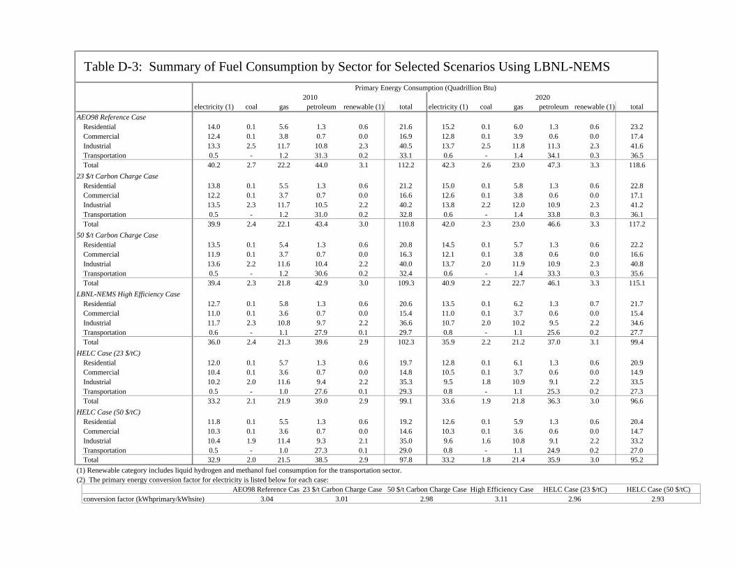
Table D-3: Summary of Fuel Consumption by Sector for Selected Scenarios Using LBNL-NEMS

Primary Energy Consumption (Quadrillion Btu)2010 2020

electricity (1) coal gas petroleum renewable (1) total electricity (1) coal gas petroleum renewable (1) total

AEO98 Reference CaseResidential 14.0 0.1 5.6 1.3 0.6 21.6 15.2 0.1 6.0 1.3 0.6 23.2Commercial 12.4 0.1 3.8 0.7 0.0 16.9 12.8 0.1 3.9 0.6 0.0 17.4Industrial 13.3 2.5 11.7 10.8 2.3 40.5 13.7 2.5 11.8 11.3 2.3 41.6Transportation 0.5 - 1.2 31.3 0.2 33.1 0.6 - 1.4 34.1 0.3 36.5Total 40.2 2.7 22.2 44.0 3.1 112.2 42.3 2.6 23.0 47.3 3.3 118.6

23 $/t Carbon Charge CaseResidential 13.8 0.1 5.5 1.3 0.6 21.2 15.0 0.1 5.8 1.3 0.6 22.8Commercial 12.2 0.1 3.7 0.7 0.0 16.6 12.6 0.1 3.8 0.6 0.0 17.1Industrial 13.5 2.3 11.7 10.5 2.2 40.2 13.8 2.2 12.0 10.9 2.3 41.2Transportation 0.5 - 1.2 31.0 0.2 32.8 0.6 - 1.4 33.8 0.3 36.1Total 39.9 2.4 22.1 43.4 3.0 110.8 42.0 2.3 23.0 46.6 3.3 117.2

50 $/t Carbon Charge CaseResidential 13.5 0.1 5.4 1.3 0.6 20.8 14.5 0.1 5.7 1.3 0.6 22.2Commercial 11.9 0.1 3.7 0.7 0.0 16.3 12.1 0.1 3.8 0.6 0.0 16.6Industrial 13.6 2.2 11.6 10.4 2.2 40.0 13.7 2.0 11.9 10.9 2.3 40.8Transportation 0.5 - 1.2 30.6 0.2 32.4 0.6 - 1.4 33.3 0.3 35.6Total 39.4 2.3 21.8 42.9 3.0 109.3 40.9 2.2 22.7 46.1 3.3 115.1

LBNL-NEMS High Efficiency CaseResidential 12.7 0.1 5.8 1.3 0.6 20.6 13.5 0.1 6.2 1.3 0.7 21.7Commercial 11.0 0.1 3.6 0.7 0.0 15.4 11.0 0.1 3.7 0.6 0.0 15.4Industrial 11.7 2.3 10.8 9.7 2.2 36.6 10.7 2.0 10.2 9.5 2.2 34.6Transportation 0.6 - 1.1 27.9 0.1 29.7 0.8 - 1.1 25.6 0.2 27.7Total 36.0 2.4 21.3 39.6 2.9 102.3 35.9 2.2 21.2 37.0 3.1 99.4

HELC Case (23 $/tC)Residential 12.0 0.1 5.7 1.3 0.6 19.7 12.8 0.1 6.1 1.3 0.6 20.9Commercial 10.4 0.1 3.6 0.7 0.0 14.8 10.5 0.1 3.7 0.6 0.0 14.9Industrial 10.2 2.0 11.6 9.4 2.2 35.3 9.5 1.8 10.9 9.1 2.2 33.5Transportation 0.5 - 1.0 27.6 0.1 29.3 0.8 - 1.1 25.3 0.2 27.3Total 33.2 2.1 21.9 39.0 2.9 99.1 33.6 1.9 21.8 36.3 3.0 96.6

HELC Case (50 $/tC)Residential 11.8 0.1 5.5 1.3 0.6 19.2 12.6 0.1 5.9 1.3 0.6 20.4Commercial 10.3 0.1 3.6 0.7 0.0 14.6 10.3 0.1 3.6 0.6 0.0 14.7Industrial 10.4 1.9 11.4 9.3 2.1 35.0 9.6 1.6 10.8 9.1 2.2 33.2Transportation 0.5 - 1.0 27.3 0.1 29.0 0.8 - 1.1 24.9 0.2 27.0Total 32.9 2.0 21.5 38.5 2.9 97.8 33.2 1.8 21.4 35.9 3.0 95.2

(1) Renewable category includes liquid hydrogen and methanol fuel consumption for the transportation sector.(2) The primary energy conversion factor for electricity is listed below for each case:

AEO98 Reference Cas 23 $/t Carbon Charge Case 50 $/t Carbon Charge Case High Efficiency Case HELC Case (23 $/tC) HELC Case (50 $/tC)conversion factor (kWhprimary/kWhsite) 3.04 3.01 2.98 3.11 2.96 2.93

TECHNOLOGY AND GREENHOUSE GAS EMISSIONS: …LBNL-42054 UC-000 EPA 430-R-98-021 TECHNOLOGY AND...

Documents

Transcript of TECHNOLOGY AND GREENHOUSE GAS EMISSIONS: …LBNL-42054 UC-000 EPA 430-R-98-021 TECHNOLOGY AND...