Technology Adoption and Factor Proportions

in Open Economies: Theory and Evidence

from the Global Computer Industry

Ana P. Cusolito Daniel Lederman∗

April 2009

Abstract

Standard theories of international trade assume that all countries usesimilar and exogenous technologies in the production of any good.This paper relaxes this assumption by allowing for the adoption ofvarious factor-complementary machines. The marriage of literatureson biased technical change and trade yields a tractable theory, whichpredicts that differences in factor endowments bias technical changetowards particular factor intensities, and thus unit factor input re-quirements vary across economies. Using data on net-exports of a sin-gle industry, computers, and factor endowments for 73 countries overthe period 1980-2000, the paper shows that once technological choicesare considered, countries with different factor endowments can becomenet exporters of the same product. (JEL Code: F1, F11, F12)

Keywords: Rybczynski; Factor Endowments; Biased TechnicalChange.

∗Development Research Group. The World Bank. The authors are grateful to WilliamF. Maloney and Pravin Krishna for helpful discussions. The research was partly fundedby the World Bank’s Latin American & Caribbean Regional Studies Program and theMulti-Donor Trust Fund.

1

1 Introduction

Theories of international trade such as the factor proportions model often

assume that countries use similar technologies in production or that techno-

logical differences are Hicks neutral. In contrast, models of biased technical

change assert that innovation and technology adoption are determined by lo-

cal factor endowments. This paper marries these two literatures. It proposes

a matching mechanism between factor endowments and technologies in open

economies, and it studies how the cross-country pattern of trade changes

once technology choices are considered.

The theory concerns economies that are open and differ in their factor

endowments. Economies are composed of multiple goods, which can be pro-

duced with a range of factor-complementary machines. These machines are

traded in a global market, which is characterized by a monopolistic com-

petitive structure. The model is tractable even though it predicts that unit

factor input requirements within industries vary across countries.

The econometric analysis utilizes data on factor endowments and net-

exports of computers and components, an industry that has received much

attention in the technology adoption and growth literature. The data set cov-

ers 73 countries during 1980-2000. The empirical model tests for the existence

of multiple technological country groups in the data, and estimates the fac-

tor proportions model in a two-stage estimation procedure. The technology

selection function is modeled as an Ordered Probit. The trade specialization

equation follows closely the standard specification of Rybczinski functions

found in the trade literature.

The econometric results suggest the existence of up to four distinct tech-

nological groups that differ in terms of their unit factor input requirements

in the production of computers. The evidence rejects the hypothesis that

the set of estimated Rybczinski coefficients are statistically equivalent across

technological country groups.

The paper is organized as follows. Section 2 discusses the related liter-

ature. Section 3 introduces the model. Section 4 solves the equilibrium of

the model. Section 5 presents the empirical strategy. Section 6 discusses the

empirical results. Section 7 concludes.

2

2 Related Literature

At least two distinct literatures are related to our model and empirical appli-

cation. The first one is the trade literature on factor proportions and trade

patterns. The second one concerns biased technical change.

2.1 Trade and factor proportions

This literature can be divided into two different strands of research. One ex-

plores the implications of the factor proportions theory under the assumption

that all countries have access to the same technologies. A second literature

conducts the same analysis but assumes that there are Hicks-neutral tech-

nology differences across countries.

In the first strand of research, Harrigan[14] examines the production side

of the factor proportions model. The author employs manufacturing outputs

and factor endowments data for up to 20 OECD countries during 1970-1985.

The most robust evidence suggests that capital abundance is a source of

comparative advantage in most of the sectors, but the effects of skilled- and

unskilled-labor are not clear. The sign of the Rybczynski coefficients change

across econometric specifications. In particular, under the time-varying pa-

rameter model, which yields the most precise coefficient estimates, skilled-

labor is a modest source of comparative advantage in only two industries (Iron

and Steel, and Fabricated Metal Products), while it is a source of compara-

tive disadvantage in the other sectors. Its largest negative effect is observed

in the Food industry. By contrast, unskilled-labor has positive effects on in-

dustry output in six of the nine industries, while land has a negligible effect

in all the manufacturing sectors.

In the same vein, but motivated by a slightly different question, Schott[25]

investigates whether developed and developing countries specialize in differ-

ent subsets of products as a result of their differences in factor endowments.

He proposes a methodology that distinguishes single- from multiple-cone

equilibria and allows for the effect of factor accumulation on a given sector’s

output to vary with a country’s endowments. Schott[25] uses value-added,

capital stock, and employment data from UNIDO for up to 45 developed and

developing countries across 28 manufacturing industries in 1990. The find-

ings reject the single-cone framework in favor of a two-cone model with labor-

3

abundant countries producing relatively little of the most capital-intensive

goods. Interestingly, the estimated development paths for industries such as

Transportation, Food, Electrical Machinery and Machinery display a twin-

peaked pattern, thus suggesting that within these sectors labor-abundant

countries produce the less capital-intensive goods, while capital-abundant

economies specialize in the production of the most capital-intensive prod-

ucts.

A paper that also belongs to this literature is Romalis[24]. The author

examines how factor proportions determine the structure of commodity trade

by integrating a many-country version of a Heckscher-Ohlin model with a

continuum of goods with Krugman[18]’s model of monopolistic competition

and transport costs. Two main predictions emerge from this work. The

first one tells that countries capture larger shares of world production and

trade of commodities that more intensively use their abundant factors. The

second prediction shows that countries that rapidly accumulate a factor see

their production and export structures systematically shift towards industries

that intensively use that factor.

In the second strand of the trade literature, Harrigan[15] provides the first

empirical test of the factor proportions theory in a framework that accounts

for international technology differences. To estimate this model, the author

uses manufacturing output shares and factor endowments data for up to 10

developed countries across 7 industries with data from 1970-1988. The most

reliable inferences across sectors that can be obtained from this study are

roughly consistent with Leamer[19] and Harrigan[14]. Specifically, the results

indicate that capital and medium-educated workers are associated with larger

GDP output shares in most of the seven industries (Food, Apparel, Paper,

Chemicals, Glass, Metals and Machinery); while non-residential construction

and high-educated workers are related to lower output shares.

Harrigan[15] improves substantially upon previous empirical frameworks,

but his implementation has the disadvantage that the model does not ex-

ploit cross-country variation to help identify the effect of factor supplies on

specialization because it only uses data on OECD countries, which tend to

have similar factor endowments and sectoral output shares. To overcome this

drawback, Harrigan and Zakrajsek[16] extend that study and work with a

larger sample, which includes data for up to 28 OECD and non-OECD coun-

4

tries and 12 industries from 1970-1992. Their evidence favors the neoclassical

theory. In Food, Wood-Paper and Oil-Coal capital abundance reduces output

shares while labor abundance raises them; Fabricated Metals and Machinery

sectors are capital intensive but not land intensive. The impact of factor en-

dowments on the Apparel-Textile sector is difficult to ascertain because the

signs of the estimated coefficients change across specifications. The between

(cross-sectional) estimates confirm the intuition about this sector, namely

that countries that are land and capital scarce but labor abundant special-

ize in this industry. The country fixed-effects estimates however show that

increases in skilled-labor over time reduce output.

In a related work, Fitzgerald and Hallak[12] estimate the effect of factor

proportions on the pattern of manufacturing specialization in a cross-section

of OECD countries, taking into account that factor accumulation responds

to productivity. The author show that the failure to control for produc-

tivity differences produces biased estimates. Their model explains 2/3 of

the observed differences in the pattern of specialization between the poorest

and richest OECD countries. However, because factor proportions and the

pattern of specialization co-move in the development process, their strong

empirical relationship is not sufficient to determine whether specialization is

driven by factor proportions, or by other mechanisms also correlated with

level of development.

Using the framework proposed by Harrigan[14], but concerned with ana-

lyzing the role of factor endowments on specialization dynamics, Redding[23]

utilizes distribution dynamics to explore this issue. In his framework, a coun-

try’s pattern of specialization at any point in time is characterized by the

distribution of shares of GDP across industries. Its dynamics are represented

by the evolution of the entire cross-sectional distribution over time. To im-

plement the model Redding[23] employs data on 20 industries in 7 OECD

countries from 1970-1990. A comparison of GDP shares between 1970 and

1990 reveals substantial variation across sectors and countries. For example,

the share of manufactures in GDP declines in all countries, although the rate

of decline varies considerably across economies, from a decline of 30.6% in

the United Kingdom to 10.1% in Denmark. There are also notable changes

in the relative importance of individual sectors within manufacturing. Some

sectors (e.g. Textiles and Ferrous metals) declined while others (e.g. Drugs

5

and Radio/TV) rose. The rate of decline or increase varies noticeably across

countries. For example, in Radio/TV, the rate of increase ranges from 19.8%

in the United Kingdom to 62.5% in Japan and 297.6% in Finland.

Perhaps more importantly, Redding[23] concludes that in the short run,

common cross-country effects such as technology progress are more impor-

tant in explaining observed changes in specialization than factor endowments

for the majority of the countries. Over longer periods, factor endowments

become relatively more important, and in the infinite horizon, factor en-

dowments account for most of the observed variation in specialization. This

evidence is in line with the idea that changes in relative factor abundance

occur gradually and take time to impact on outputs structures.

Overall, the factor proportions model provides a story about static and

dynamic specialization around the world. Some evidence shows that tech-

nological differences across countries can produce similar patterns of special-

ization in spite of large differences in factor endowments (Schott[25]). Our

model extends the standard factor-proportions theory to allow for technology

differences across countries.

2.2 Biased technical change

This literature concerns the hypothesis that countries use different factor-

complementary machines to produce the same products. This strand of re-

search can also be divided into two different approaches. The first one as-

sesses whether factor shares vary systematically with the level of development

(e.g. Young[26], Gollin[13], Bernanke and Gurkaynak[3], and Ortega and

Rodriguez[21]). The second investigates whether complementarities between

inputs and technology bias technical change (e.g. Acemoglu[1], Caselli[6]).

The first literature initially found that labor shares in national income

vary widely, ranging from 0.05 to 0.80 in international cross-sectional data

(e.g. Elias[10] and Young[26]). Gollin[13] questioned these estimations by

arguing that the widely used approach, which is based on Cobb-Douglas pro-

duction functions, tends to underestimate the labor income of self-employed

workers, and the corrected labor shares fall in the range of 0.65 to 0.80.

This evidence was later reaffirmed by Bernanke and Gurkaynak[3], but re-

jected by Ortega and Rodriguez[21]. The later uses industrial survey data

to explore the same question, and controlling for the measurement problem

6

of self-employed workers it found a significant negative cross-sectional rela-

tionship between capital share and per capita income within industries. In

a related paper, Dobbelaere and Mairesse[9], find that imperfections in the

product and labor markets generate a wedge between factor elasticities in

the production function and their corresponding shares in revenue, both at

firm and industry level.

In the second approach, Acemoglu[1] shows how cross-country differences

in factor endowments can bias technical change. In his framework, two forces

shape technical change, price and market-size effects. The price effect reflects

the incentives to generate technologies that create more expensive goods. The

second effect captures the incentives to produce technologies for which there

is a big market. While the former encourages innovations to complement

scarce factors, the latter leads to technical change favoring abundant fac-

tors. The elasticity of substitution between two different factors determines

how powerful these effects are. In the long run, technical change favors the

abundant factor if the elasticity of substitution is sufficiently large.

Evidence of complementarities between factors of production and technol-

ogy has been provided by Caselli[6], who explored the relationship between

factor endowments and the composition of capital imports. The author finds

that human-capital abundant countries devote a larger share of their in-

vestment to acquire complex technologies, which can only be employed by

skilled-workers.

We depart from the neo-classical trade literature by relaxing the assump-

tion of Hicks neutral technologies, and by allowing countries to make their

own technology choices. We complement the biased-technical change litera-

ture by analyzing how countries’ technology choices alter the impact of factor

endowments on trade.

3 The Model

Let c=1 , . . . , C index countries, let f =1 , . . . , F index factors,

and let j= 1 , . . . , J index industries. Assume that countries are open.

Output of industry j in country c, Y cj , can be written as a constant elasticity

of substitution (CES) production function of factor inputs f, V cjf , and factor-

f -complementary machines, Acjf . Thus,

7

Y cj = [

F∑f=1

γf (Ac1−βj

jf V cβj

jf )σj−1

σj ]σj

σj−1 . (1)

γf ∈ (0, 1) is a distribution parameter that captures how important factor f is

in the production process. Specifically, we assume∑F

f=1 γf = 1. Parameter σj

is the elasticity of substitution between two factors and Acjf has the following

functional form:

Acjf = [

∫ NWf

0ac

jf (i)αdi]

1α . (2)

NWf stands for the number of varieties of factor-f -complementary machines

available in the global market, and acjf (i) for the units of variety i. Parameter

α determines the elasticity of substitution between any two varieties of such

machines.

Final goods producers face a two-stage decision process. First, they decide

how many units of each factor of production to hire. Second, they choose

how many machines to buy to complement each factor. In doing so, they

take technology prices as given, because countries are small. The machines

belong to the category of general purpose technology, and they can be used

in different sectors. The world’s technological market has a monopolistic

competitive structure. Each monopolist from country x, with x = 1, ..., C,

that produces technology to complement factor f sets a rental price pc,xjf (i)

per unit of machine i supplied to firms of industry j in country c. She faces a

production cost, µxf , and a transport cost, τ c,x

f , per unit of invented machine

she sells to firms in country c.

4 Equilibrium

To find the equilibrium of the model we proceed in the following manner.

First, we solve the equilibrium for a representative sector. Second, we char-

acterize the equilibrium for the whole economy. To solve the equilibrium for

a sector we need to find the solutions to the final good producers’ problem

and technology suppliers’problem. This is presented in the following sections.

8

4.1 Final Good Producers

Firms choose how many machines to buy in order to complement each pro-

duction factor.1 The problem for a representative firm in sector j can be

written as follows:2

min{acfj

(i)}{F∑

f=1

[∫ NW

f

0pc,xi

jf (i)acjf (i)di]} (3)

subject to the following constraints:

1. [∑F

f=1 γf (Ac1−βj

jf Qcβj

fj )σj−1

σj ]σj

σj−1 ≥ 1

2. Acjf = [

∫ NWf

0 acjf (i)

αdi]1α

The first order conditions for problem (3) deliver the following expression for

the demand of machine i that complements factor z per unit of output:

acjz(i) =

Ecz

P cjz

pc−ε

jz (i)

P c−ε

jz

. (4)

Ecz represents the expenditures that country c devotes to complement factor

z, P c1−ε

jz ≡∫ NW

z0 pc1−ε

jz (i)di, and ε ≡ 11−α

is the elasticity of substitution be-

tween two varieties of machines z.34 Equation (4) implies that the demand

of machine i is an increasing function of real expenditure on technology z,Ec

z

P cjz

, and a negative function of the price of the machine, pcjz(i).

Given the demand for machines, firms minimize unit cost functions to

determine the optimal unit factor input requirements. Specifically, they solve

the following problem:

min{V cfj}f=1,...,F

{F∑

f=1

wcfV

cfj} (5)

subject to the following constraints:

1We solve the model backward because producers are rational agents.2For the sake of simplicity firms’ subindexes are omitted.3For the sake of simplicity we assume that Ec

z is given.4See the Appendix for the complete proof.

9

1. [∑F

f=1 γf (Ac1−βj

jf Qcβj

fj )σj−1

σj ]σj

σj−1 ≥ 1

2. Acjf = [

∫ NWf

0 acjf (i)

αdi]1α

3. acjz(i) = Ec

z

P cjz

pc−ε

jz (i)

P c−εjz

,

where wcf stands for the cost per unit of factor f in country c. In the op-

timum, the marginal product of each factor equals its marginal cost. From

the optimal conditions we can obtain the optimal Qcjf :

Qcjf = Ac

−(1−βj)

βj

jf {F∑

z=1

γz[(Ac

jz

Acjf

)σj

σj(1−βj)+βj (wc

fγz

wczγf

)σjβj

σj(1−βj)+βj ](σj−1)

σj }−σj

(σj−1)βj . (6)

wcf is the cost per efficiency unit of factor f. Equation (6) shows that factor-

f -complementary machines affect unit factor input requirements through two

opposing effects. On the one hand, larger values of Acjf increase the produc-

tivity of the factor and reduce its requirements. On the other hand, factor f

becomes relatively more productive than other factors, which increases firms’

incentives to hire more units. The sign of the net-effect depends on which ef-

fect dominates. Lower values of wcf (γz), and increasingly negative (positive)

differences between wcf (γf ) and wc

z (γz), for z 6= f and z = 1, ...F , make the

second effect more prominent.

4.2 Technology Suppliers

Recall that any monopolist localized in country x faces a marginal cost µxzτ

c,xz

for manufacturing and delivering one unit of technology z to country c.5 The

profits of this monopolist supplying machine i to country c are as follows:

πc,xjz (i) = [pc,x

jz (i)− (µxzτ

c,xz )]

Ecz

P cjz

pc−ε

jz (i)

P c−ε

jz

. (7)

Maximization of equation (7) with respect to pc,xjz (i) delivers the following

optimal price,

5Since we are not concerned with modeling the innovation-entry decision, we assumethe number of innovators is exogenously given.

10

pc,xjz (i) = (µxi

z τ c,xiz )(

ε

ε− 1), (8)

which is a constant markup over the marginal cost of producing and trans-

porting a unit of technology. This markup depends negatively on the elas-

ticity of substitution between varieties of z -machines. Inserting equation (8)

into (4) gives the solution for acjz(i),

acjz(i) = (

ε− 1

ε)

Ecz(µ

xiz τ c,xi

z )−ε∫ NWz

0 (µxnz τ c,xn

z )1−εdn. (9)

Inserting equation (9) into (2) provides the solution for Acjz,

Acjz = (

ε− 1

ε)

Ecz

NWz

[∫ NW

z

0(µxn

z τ c,xnz

NWz

)1−εdn]1

ε−1 . (10)

To finish characterizing the equilibrium for this sector, we insert equation

(10) into (6) to obtain the final expression for Qcjz,

Qcjz = {(ε− 1

ε)

Ecz

NWz

[∫ NW

z

0(µxn

z τ c,xnz

NWz

)1−εdn]1

ε−1}−(1−βj)

βj Υc

−σj(σj−1)βj

jz (11)

where

Υcjz = {

F∑f=1

γf [(Ec

f

Ecz

)(

∫ NWf

0 (µxnz τ c,xn

z )1−εdn∫ NWz

0 (µxmz τ c,xm

z )1−εdm)

1ε−1 ]

σjσj(1−βj)+βj (

wczγf

wcfγz

)σjβj

σj(1−βj)+βj }σj−1

σj .

(12)

A comparison of equation (11) with the neo-classical factor proportions model

reveals that cross-country differences in technology prices are a source of

cross-country variation in unit factor input requirements. This result consti-

tutes an important departure from the model with Hicks neutral technology.

4.3 The Economy

To analyze how technology choices affect the impact of factor endowments

on trade, we need to solve the equilibrium for the whole economy. Employing

11

matrix notation, we define Qc as the matrix of unit factor input requirements

for economy c. Market clearing conditions in this economy are as follows:

QcYc = Vc, (13)

where Yc is the vector of sectoral outputs and Vc is the vector of factor

endowments. Assuming that the number of goods is equal to the number

of products, and denoting by Rc the inverse of matrix Qc, it is possible

to express output of country c as a linear function of country c’s factor

endowments. Specifically,

Yc = RcVc. (14)

If countries can be clustered in K groups, such that two countries belong

to the same group if they make identical technology choices, we can express

output of country c, which belongs to group k, Yc,k, with k = 1, ..., K, and

worldwide output, Yw, as follows:

Yc,k = RkVc,k (15)

and

Yw =K∑

k=1

RkVw,k, (16)

respectively. Vw,k is the vector of factor endowments of group k. Denoting

by TBc the trade balance of country c and by sc country c’s share of world

consumption, net-exports of this economy are

NXc = Yc − scYw = Rk(Vc,k − scV

w,k)−K∑

z=1,z 6=k

RzscVw,z. (17)

The previous system provides the following estimating equation for the net-

exports in sector j by country c, which belongs to technology group k :

NXc,kj =

F∑f=1

rkfj(V

c,kf − scV

kf ) +

K∑z=1,z 6=k

F∑f=1

rzfj(−scV

zf ). (18)

12

A comparison of equation (18) with the standard Rybczynski equation sug-

gests that the concept of relative abundance of a factor in a country must be

redefined when technology choices are introduced in the standard factor pro-

portions model. Notably, a country’s factor abundance is measured relative

to the aggregate endowment of the technological group to which it belongs.

5 Empirical Strategy

This section presents an empirical implementation of our theory. We focus

the analysis on the computer sector because it has received much attention

in the technology adoption and growth literature. The section is structured

as follows. First, we present the estimating procedure. Second, we describe

the indicators and proxies we construct to test the theory. Third, we provide

a preliminary analysis of the data.

5.1 Estimating procedure

The theoretical framework motivates an empirical model with two equations

because net-exports determination is governed by different sets of parameters,

and the set of parameters which determine a particular country’s net-exports

depend on the technological group to which it belongs. The most efficient

method to estimate this model is the Full-Information Maximum Likelihood

(FIML) estimator (see Chiburis and Lokshin[7]). However, we employ a less

efficient method, the Two-Step approach. An implication of using the last

technique is that it increases the chance of rejecting our theory.

In the first step, we estimate an Ordered-Probit equation, and we cluster

countries across technological groups. To find the locations of the cut-off

points that split the sample between technological regimes, we proceed in the

following manner. First, we assume the sample splits in a particular number

of groups i.e., 2, 3, or 4. Second, we follow the methodology implemented by

Hotchkiss[17], which consists in estimating the model for every reasonable

cut-off parameter. We start the process dividing the sample in a way that

delivers the maximum number of groups with no more than 10% of the

observations per each one. This provides the highest degree of freedom to

13

move the cut-off points along the range of possible values.6 Then we estimate

the first step.

In the second step, we estimate the Rybczynski coefficients for each tech-

nological group. We use the OLS approach but we control for selection.7

Finally, we apply the goodness of fit criterium to identify the set of esti-

mated parameters that yields the least sum of squared residuals.

The first stage of the econometric model can be written as:

Rct = ΘZc

t + µct (19)

Rct =

0 if −∞ < Rct ≤ R1t

1 if R1t < Rct ≤ R2t

.

.

.

K − 1 if RK−1t < Rct ≤ ∞,

where Rct is a continuous variable that we construct to cluster countries across

technological groups. This variable is intended to capture the technology

choices that countries make. The following section explain the methodology,

the variables, and the economic arguments we employ to build it. Θ is a

vector of parameters, and Zct is a vector that includes some of the variables

we use to build Rct . In particular, these variables are: stock of capital, labor,

and intellectual property rights (IPRs) of each country, as well as weighted

averages of the stock of capital, labor, and IPRs of its technology suppliers.

µct is a standard normal shock, and R1t, R2t, ..., RK−1t are the unknown cut-

off points, which satisfy the following condition: R1t< R2t<, ...,< RK−1t. We

also define R0t ≡ −∞ and RKt ≡ ∞ to avoid having to handle the boundary

cases separately.

The second-stage Rybczynski equation is:

6The cut-off points are moved in steps of 1 percentile of the continuous variable weemploy to cluster countries across technological regimes.

7Specifically, we introduce the estimated λci ≡

φ(Rk−Rc)−φ(Rk+1−Rc)

Φ(Rjk+1−Rc)−Φ(Rk−Rc)as an explanatory

variable of the Rybczynski equation corresponding to regime i.

14

NXc,kt = r0 +

F∑f=1

rkf (V

c,kft − scV

kft) +

F∑f=1,z 6=k

rzf (−scV

zft) + υc,k

t (20)

NXct =

NXc,k0t if Rc

t = 0

NXc,k1t if Rc

t = 1

.

.

.

NXc,K−1t if Rc

t = K − 1,

where NXc,kt are the net-exports of computers for country c which belongs

to group k in period t. rkf is the Rybczynski coefficient for factor f in tech-

nological group k. We include four factors of production: stock of capital,

skilled-labor, unskilled-labor, and arable land. Given that in the economy

there are more than four sectors, we follow the trade literature and we as-

sume that the constant term, r0, captures the mean effect of omitted factors.8

The model relies on the following assumptions: A1. υc,kt ∼ N(0, σ2

υ,k), for

k = 1, ..., K; A2. µct ∼ N(0, 1); A3. σ2

υ,kz = 0, for k 6= z and k, z = 1, ..., K;

A4. σ2υ,µ 6= 0.

As we mention at the beginning of this section, we estimate equations (19)

and (20) using the Two-Step approach, which is less efficient than the FIML

method. This implies that if we find evidence in line with our predictions,

our theory is very robust. However, evidence against the theoretical results

is not enough to reject the theory.

5.2 Indicators and proxies

This section describes the proxies we construct to estimate equations (19)

and (20). It also documents the sources of data we employ for such purpose.

8See Fitzgeral and Hallak[12], Harrigan[14], and Reeding[23] among others.

15

5.2.1 The technology selection variable

To construct variable Rct we rely on equation (10), which shows that the

amount of machines that a country buys to complement a particular factor of

production is a function of the marginal cost of manufacturing one machine,

the transport cost, and the elasticity of substitution between two varieties of

the same type of equipment.

The marginal cost of producing one unit of a machine is a function of the

factor endowments of the country that supplies the equipment because they

determine the prices of the inputs involved in the process. As our empirical

implementation focuses on the computer sector, which is one of the most

technologically advanced industries, we assume that to produce a computer,

a country needs to acquire machines from the same sector. These equip-

ments complement different factors of production, and they can be acquired

domestically or imported from abroad. Therefore, the technology choices of

a country are a function of its factor endowments as well as the weighted

averages of the factor endowments of its technology suppliers, where each

weight accounts for the transport cost, and is define as the inverse of the

distance between the country that buys and the one that sells the machine.

Technology choices can also be affected by the IPRs of innovators’ coun-

tries. One reason to justify this statement is that inventors of countries with

weak IPRs may have incentives to provide more sophisticated and expen-

sive technologies to avoid imitation. Another argument is that strong IPRs

can encourage monopolists to charge a higher mark-up because they face no

competition. In any case, a country’s technology choice can also depend on

its own IPRs as well as the inverse-distance-weighted average of the IPRs of

its technology suppliers.

Once we identify the variables that affect countries’ technology choices,

wee proxy variable Rct with the predicted value for the principal factor in

a principal component analysis of these variables (stock of capital, labor,

arable land, and IPRs of each country as well as the corresponding distance-

weighted averages of its technology suppliers).

The sources of data we employ to construct Rct are the following. Data

on capital stocks come from Serven and Calderon[25], who extend the se-

ries provided by Penn-World Tables, version 5.6, using the perpetual inven-

tory method. The labor force is from the International Labor Organization

16

(ILO). The endowment of arable land comes from the World Bank’s World

Tables. Data on intellectual property rights protection come from Park and

Ginarte[22], who construct an index of patent rights using a coding scheme

applied to national patent laws. Five categories of the patent laws were

examined: (1) extent of coverage, (2) membership in international patent

agreements, (3) provisions for loss of protection, (4) enforcement mecha-

nisms, and (5) duration of protection. Each of these categories (per country,

per time period) was scored a value ranging from 0 to 1. The un-weighted

sum of these five values constitutes the overall value of the IPRP index. Bi-

lateral data on computers imports come from Feenstra et al.[11]. The data

are available at 4-digit level of the Standard International Trade Classifica-

tion, Revision 2. We consider the following categories, 7521, 7522, 7523, and

7528.9 The source for bilateral distances is the CIA World Factbook.

5.2.2 Net-exports of computers

To estimate equation (20) we need data on net-exports of computers. The

source of these data is Feenstra et al.[11]. This data set provides information

on bilateral trade flows at 4-digit level of the Standard International Trade

Classification, Revision 2. Our net-exports variable includes the following

categories, 7521, 7522, 7523, and 7528.

5.2.3 Factor endowments

To estimate the Rybczynski coefficients we need data on factor endowments.

We consider four factors: stocks of capital, skilled-labor, unskilled-labor, and

arable land. Data on capital stocks come from Serven and Calderon[25]. The

labor force is from the International Labor Organization (ILO). To calculate

endowments of high- and low-skilled labor, we use data on educational attain-

ment from Barro and Lee[2]. Skilled-workers are defined as the population

economically active which have attained at least secondary school. The rest

9Code 7521 refers to Analogue and hybrid data processing machines; code 7522 refersto Complete digital data processing machines, comprising in the same housing the centralprocessing unit and one output unit; code 7523 refers to Complete digital central processingunits, digital processors consisting of arithmetical, logical, and control elements; codes 7528refers to Off-line data processing equipment, n.e.s.

17

is considered unskilled-labor. The endowment of arable land comes from the

World Bank’s World Tables.

The resulting sample covers 73 developing and developed countries over the

period 1980-2000. Table 1 presents summary statistics of the variables de-

scribed in previous sections, and the Appendix provides a list of the countries

included for the analysis.

[Insert Table 1 about here]

5.3 Net exports of computers and endowments

A preliminary review of the data suggests that countries with notably dif-

ferent factor endowments have comparable net-exports of computers. It also

shows that countries close to each other in the ranking of factor endow-

ments are net-exporters and net-importers of computers. Table 2 displays

the countries that are located at the top and the bottom of the distribution

of countries ranked by their net-exports of computers. For each of these

economies, the table reports their capital and skilled-labor abundance.

[Insert Table 2 about here]

A comparison of columns (3) and (5) shows that within the group of top net-

exporters, there are countries such as India, China, Indonesia, and Philip-

pines, which belong to the bottom of the capital-labor ratio ranking, while

other economies such as Japan, Singapore and Korea Republic belong to the

top of such distribution. A similar observation can be derived from the com-

parison of columns (3) and (7). Among the group of top net-exporters, there

are economies such as India, Indonesia and Costa Rica, which belong to the

bottom of the skilled-labor distribution, and other countries such as Japan,

Korea Rep., and Ireland, which belong to the top of this distribution.

6 Results

We organize our discussion of the results in the following manner. First, we

analyze the statistical significance of the estimated parameters that allow us

to test the econometric specification we implement. Second, we interpret the

18

outcomes from the estimation of the selection equation. Third, we discuss

the results from the estimation of the Rybczynski equations. Table 3 presents

the estimation outputs. Each column splits the results across technological

regimes.

[Insert Table 3 about here]

6.1 Specification tests

The econometric results suggest the existence of up to four technological

regimes. Table 3 shows that the model that fits best the data is the one

with four regimes. The optimal cutoffs are found at the 35th, 50th, and

90th percentiles of the distribution of variable Rct , and they are statistically

different from zero at 1% level. Some of the estimated coefficients that correct

for selection (Lambdas) are also statistically significant at 5% level. As the

number of regimes increases, trading partners’ endowments and IPRs become

significant and rise the probability of belonging to the highest regime. This

can explain why countries such as Albania, Costa Rica, and Jamaica appear

in the third regime.

6.2 Technology selection

Table 3 shows that many of the explanatory variables are statistically signif-

icant in the three specifications. Interestingly, the results show that as the

number of technological regimes increases, the coefficients corresponding to

the endowments and IPRs of trading partners become statistically more sig-

nificant. This result has an important economic implication. As it shows that

in open economies, the adopted technologies are not necessarily the ones that

complement relatively abundant factors. The outcomes indicate that the en-

dowments and institutions of close economies are also very important. Table

4 shows the final distribution of countries across technological groups.

[Insert Table 4 about here]

6.3 Rybczynski equation

The results indicate that capital abundance is a source of comparative advan-

tage in the production of computers for countries that belong to the lowest

19

technological regimes. However, it is a source of disadvantage for countries

that belong to the highest regimes. By contrast, skilled-labor abundance is

statistically significant and has a positive impact on the net-exports of com-

puters of the highest regimes. Both results appear systematically in the three

specifications. Notably, as the number of regimes increases, unskilled-labor

abundance becomes significant and has a positive impact on the net-exports

of computers for the lowest regime, while skilled-labor abundance affects net-

exports of computers in an opposite direction. Land is significant and has a

negative effect on most regimes. This result is robust to different specifica-

tions. All these effects are statistically different from zero at 1 % level.

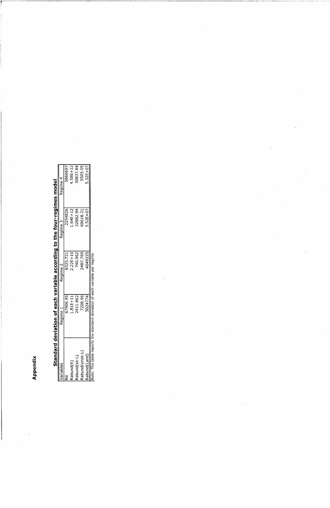
Combining information on the dependent and explanatory variables for

each technological group together with the estimated Rybczynski coefficients

of column (3) we find that a 1$ increase in the relative endowment of capital

leads to a 0.0001$ increase in the net-exports of computers of the lowest

regime, and a 0.0028$ reduction in the net-exports of the highest regime.

These effects are economically large: a 1 standard deviation increase in the

relative abundance of capital generates a 266.542 standard deviations increase

in the net-exports of the first regime, and a 7,463.15 standard deviations

reduction in the net-exports of the highest regime.10 An increase of 1 worker

in the relative abundance of skilled-labor leads to a 14.45$ reduction in the

net-exports of regime 1, and a 28.312$ and 577.65$ increment in the net-

exports of regimes 3 and 4, respectively. The economic effects are small: a 1

standard deviation increase in the relative abundance of skilled-labor delivers

a 0.513 standard deviation reduction in the net-exports of regime 1, and a

0.41- and 3.03 standard deviations increase in the net-exports of regimes

3 and 4, respectively. By contrast, an increase of 1 worker in the relative

abundance of unskilled-labor generates a 4.043$ increase in the net-exports of

regime 1. The economic effect is very modest: a 1 standard deviation increase

in the relative abundance of unskilled-labor is associated to a 0.161 standard

deviation increase in the net-exports of regime 1. Finally, an increment of 1

hectare in the relative abundance of arable land leads to a 3$ reduction of

net-exports in regime 1 and a 119$ reduction in the net-exports of regime 4.

Having presented preliminary evidence in support of our theory, we now

10See the Appendix for a description of the standard deviation of the dependent andindependent variables per technological regime.

20

move to provide a formal test of the null hypotheses that the Rybczynski

coefficients are equivalent across technological groups. Table 5 reports the

p-values corresponding to the hypothesis that the Rybczynski coefficients are

statistically equivalent.

[Insert Table 5 about here]

The Table shows that in spite the fact that we use the less efficient method

there is substantial evidence supporting our theory. The Rybczynski coeffi-

cients vary across technological groups.

7 Conclusion

The neoclassical model of trade predicts that international specialization will

be jointly determined by cross-country differences in relative factor endow-

ments and exogenous technology levels. In this paper we develop a model

that relaxes the Hicks neutral technology assumption by allowing countries to

adopt their own technologies. The marriage of literatures on biased technical

change and trade yields a tractable theory whereby differences in factor en-

dowments bias the technical change towards particular factors of production,

and thus unit factor input requirements vary across economies. Using data

on net exports of a single industry, computers, and factor endowments for 73

countries over the period 1980-2000 we test the theory. The descriptive and

econometric evidence suggests that once technological choices are considered,

countries with different factor endowments can become net exporters of the

same product.

References

[1] Acemoglu, D., 2002. Directed Technical Change. Review of Economic

Studies, 7 (4), 781-809.

[2] Barro, R. and L., Jong-Wha, 1993. International Comparisons of Edu-

cational Attainment. Journal of Monetary Economics, 32 (3) 363-394.

21

[3] Bernanke, B.S. and R.S., Gurkaynak, 2002. Is Growth Exogenous? Tak-

ing Mankiw, Romer, and Weil Seriously, B.S. Bernanke and K. Ro-

goff (eds.) NBER Macroeconomics Annual 2001 (Cambridge, MA: MIT

Press), 11-57.

[4] Bernstein, J. and D., Weinstein, 2002. Do Endowments Determine the

Location of Production? Evidence from National and International

Data. Journal of International Economics, 56 (1), 55-76.

[5] Calderon, C., and L, Serven, 2004. Trends in Infrastructure in Lat-

ing America, 1980-2001. World Bank Policy Research Working Paper

N 3401.

[6] Caselli, F. and J., Wilbur, 2001. Cross-Country Technology Diffusion:

The Case of Computers. American Economic Review P & P. 91 (2),

328-335.

[7] Chiburis, R. and M., Lokshin, 2007. Maximum Likelihood and Two-Step

Estimation of an Ordered-probit Selection Model. The Stata Journal. 7

(2), 167-182.

[8] Davis, D. and D., Weinstein, 2001. An Account of Global Factor Trade.

American Economic Review, 91 (5),1423-54.

[9] Dobbelaere, S. and J., Mairesse, 2008. Panel Data Estimates of the Pro-

duction Function and Product and Labor Market Imperfections. NBER

Working Paper N. 13975.

[10] Elias, V., 1992. Sources of Growth: A Study of Seven Latin American

Economies. San Francisco: ICS Press.

[11] Feenstra, R., Lipsey, R. and H., Bowen, 1997. World Trade Flows, 1970-

1992, with Production and Tariff Data. NBER WP ] 5975.

[12] Fitzgeral, D., and J.C., Hallak, 2004. Specialization, Capital Accumu-

lation, and Development. Journal of International Economics, 64(2),

277-302.

[13] Gollin, D., 2002. Getting Income Shares Right. Journal of Political Econ-

omy, 90, 458-474.

22

[14] Harrigan, J., 1995. Factor Endowments and the International Location

of Production: Econometric Evidence from the OECD, 1970-1985. Jour-

nal of International Economics, 39 (1/2), 123-141.

[15] Harrigan, J., 1997. Technology, Factor Supplies and International Spe-

cialization: Testing the Neoclassical Model. American Economic Review,

87 (4), 475-494.

[16] Harrigan, J. and E. Zakrajsek, 2000. Factor Supplies and Specialization

in the World Economy. NBER Working Paper 7848.

[17] Hotchkiss, J., 1991. The Definition of Part-Time Employment: A

Switching Regression Model with Unknown Sample Selection. Interna-

tional Economic Review, 32 (4), 899-917.

[18] Krugman, P., 1980. Scale Economies, Product Differentiation, and the

Pattern of Trade. American Economic Review, 70 (5), 950-959.

[19] Leamer, E., 1984. The Commodity Composition of International Trade

in Manufactures: An Empirical Analysis. Oxford Economic Papers, 26,

350-374.

[20] Leontief, W., 1956. Factor Proportions and the Structure of American

Trade: Further Theoretical and Empirical Analysis. Review of Eco-

nomics and Statistics, 38, 386-407.

[21] Ortega, D. and F., Rodriguez, 2003. Are Capital Shares Higher in Poor

Countries?. Working Paper.

[22] Park, W. and J.C., Ginarte, 1997. Determinants of Patent Rights: A

Cross National Study. Research Policy N26 (3), 283-301.

[23] Redding, S., 2002. Specialization Dynamics. Journal of International

Economics, 58, 299-334.

[24] Romalis, J. 2004. Factor Proportions and the Structure of Commodity

Trade. American Economic Review, 94 (1), 67-97.

[25] Schott, P., 2003. One Size Fits All? Theory, Evidence and Implications

of Cones of Diversification. American Economic Review, 93 (3), 686-708.

23

[26] Young, A. 1995. The Tyranny of Numbers: Confronting the Statistical

Realities of the East Asian Growth Experience. Quarterly Journal of

Economics, 100, 641-80.

24

8 Appendix

Proof first stage of FGP’s problem

The first order condition for variety i is

pcjz(i) =

∂Acjz

∂acjz(i)

K[Φ1jz(i) + Φ2

jz(i) +F∑

f=1;f 6=z

Φ3jfz(i)] (21)

where

Φ1jz(i) = γz(1− βj)

(σj − 1)

σj

Ac(1−βj)

(σj−1)

σj−1

jz Qcβj

(σj−1)

σj

jz (22)

Φ2jz(i) = γzβj

(σj − 1)

σj

Ac(1−βj)

(σj−1)

σj

jz Qcβj

(σj−1)

σj−1

jz

∂Qcjz

∂Acjz

(23)

Φ3jfz(i) = γfβj

(σj − 1)

σj

Ac(1−βj)

(σj−1)

σj

jz Qcβj

(σj−1)

σj−1

jz

∂Qcjf

∂Acjz

(24)

K = λσj

(σj − 1)[

F∑f=1

γf (Ac1−βj

jf V cβj

jf )σj−1

σj ]σj

σj−1−1

(25)

and λ is the shadow price of the constraint. Since [Φ1jz(i) + Φ2

jz(i) +∑Ff=1;f 6=z Φ3

jfz(i)] = [Φ1jz(n) + Φ2

jz(n) +∑F

f=1;f 6=z Φ3jfz(n)], we can divide the

first order condition for variety i by that for variety n and obtain the follow-

ing expression

pcjz(i)

pcjz(n)

=

∂Acjz

∂acjz(i)

∂Acjz

∂acjz(n)

=a

c−(1−α)jz (i)

ac−(1−α)jz (n)

(26)

Multiplying both size of equation (21) by pcjz(i) and integrating over i, we

obtain the following result

acjz(i) =

Eczp

c−ε

jz

P c1−ε

jz

(27)

where Ecz ≡

∫ NWz

0 pcjz(i)a

cjz(i)di.

25

Variable Obs Mean Std.Dev Min Max

Net_Exports 365 1.70E+04 2.58E+06 -3.11E+07 1.32E+07Stock_of_K 365 7.94E+11 2.16E+12 1.58E+09 2.13E+13Unskilled_Labor 365 1.39E+04 5.06E+04 6.59E+01 4.14E+05Skilled_Labor 365 7.69E+03 2.65E+04 1.42E+01 2.58E+05Land (hect.) 365 1.30E+07 3.19E+07 1.00E+03 1.89E+08IPRP 365 2.30E+00 1.24E+00 0.00E+00 4.88E+00IPRP_of_Trading Partners 365 7.06E-02 1.25E-01 3.23E-04 7.94E-01

Country Net-Exports Ranking Capital/ Labor Ranking Skilled Lab/ Labor RankingChina 1.24E+07 73 1.45E+07 23 38.4 37Malaysia 1.18E+07 72 5.76E+07 47 50.5 49Singapore 1.05E+07 71 2.03E+08 71 59.1 57Korea Rep. 9187286 70 2.42E+08 73 75.3 69Philippines 6350562 69 1.61E+07 26 53.6 51Ireland 5953102 68 1.04E+08 53 64.1 59Japan 5000000 67 1.85E+08 69 71.9 66Mexico 4675278 66 4.48E+07 45 40.3 38Indonesia 2329506 65 1.61E+07 25 26.8 24India 33958 64 7649168 16 22.2 18Costa Rica 21775 63 1.99E+07 30 29.9 30Min. 21775 7.65E+06 22.2Max. 12400000 2.42E+08 75.3Mean 6204679 4.48E+07 50.5Std.Dev. 4384442 8.71E+07 18.2Austria -1029426 11 1.65E+08 68 70.1 63Denmark -1196473 10 1.44E+08 62 68.1 62UK -1200000 9 1.11E+08 54 58.2 56Sweden -1592865 8 1.32E+08 58 80.3 71Spain -1613921 7 1.13E+08 56 46.9 44Switzerland -2773254 6 2.03E+08 72 71.0 65Australia -3062108 5 1.48E+08 64 73.4 68France -3942278 4 1.52E+08 65 55.7 54Italy -4117605 3 1.53E+08 66 46.7 43Canada -5744931 2 1.40E+08 60 79.6 70USA -3.11E+07 1 1.60E+08 67 89.7 73Min. -31100000 1.11E+08 46.7Max. -1196473 2.03E+08 89.7Mean -5634344 1.48E+08 70.1Std.Dev. 9069688 2.53E+07 13.9

Note: This table reports the values of net-exports of computers, capital-labor ratios, and skiiled_labor-labor ratios for the countries located at the top and the bottom of the distribution of countries ranked according to their net-exports of computers during the year 2000. Figures corresponding to net-exports are measrued in nominal of U.S dollars. Figures for the skilled-labor/labor are measured in percentage units.

Table 2. Net Exporters and Factor Endowments

Table 1. Summary Statistics