Technological advances to improve the quantification of ...

vEGU21

Technological advances to improve the quantification

of volcanic emissions

Christopher Fuchs1, Jonas Kuhn1,2, Nicole Bobrowski1,2 and Ulrich Platt1,2

1Institut of Environmental Physics, Heidelberg, Germany2Max Planck Institute for Chemistry, Mainz, Germany

GI6.1: Remote sensing for environmental monitoring, EGU21-1308, 29 April 2021

[email protected]

vEGU21 Christopher Fuchs, GI6.1, EGU21-1308, 29 April 2021 1

Imaging trace gases in volcanic emissions

Why monitoring volcanic trace gas emission?

• Changes in emission fluxes (e.g. CO2, SO2) can indicate changes in the volcanic activity• Variations in emission ratios (e.g. SO2/BrO) can identify changes in the volcanoes' magmatic system• Insights into trace gas concentration distributions to better understand atmospheric chemistry (e.g. halogens)

➔ Facilitating volcanic monitoring & activity assessment and increase understanding in atmospheric chemistry

Prerequisites for the imaging technique?

➔ Resolve plume processes at their intrinsic time and spatial scales

1. Differentiation between numerous trace gases → use characteristic differential absorption structures

2. Sufficient selectivity and sensitivity→ spectral resolution in the “sub nm” scale

3. Quantification on concentration distributions→ column densities (CDs, number density of trace gas along light path)


Applied imaging techniques

Imaging DOAS

2D detector: one dimension for spatial information, other dimension for spectral information → scanning required for a 2D column density image

High spectral informationdetection of various trace gas species simultaneously

Too slow due to scanninglimited light throughput + complex scanning mechanism

acquisition time in the order of minutes

SO2 UV-cameras

2D detector solely used for spatial information → spectral selection by wavelength selective elements (e.g. spectral filter using 2 spectral channels exploiting broad band absorption)

High spatio-temporal resolutionplume propagation direction from images; flux monitoring

Low spectral selectivity and high cross interferencesonly for high SO2 CDs due to broadband interference withwith clouds, aerosols and ozone

Louban et al., 2009

SO2 CD

BrO CD

volcanicplume

volcanicplume

SO2 CD image@ 1 fps & 1 MP

channel A channel B

≈ 25 nm gap

broadbandinterference

Lübcke et al., 2013

By selecting appropriate FPI quantities (n, d, R, α) the FPIs’ transmission spectrum can be matched to periodic absorption features of the investigated trace gas (here: SO2)

Transmission at max.SO2 absorption(on-band, setting A)

Transmission at min. SO2 absorption(off-band, setting B)

➔ High specificity to the trace gas by using narrowband structures and reduction in broad band interferences due to small spectral shift of ≈ 1 nm (20 nm for SO2 UV-cameras)

Application of an Fabry-Perot interferometer (FPI) as wavelength selective element

Radiation traversing an FPI undergoes multiple reflections causing either constructive or destructive interference resultingin a comb shaped transmission spectrum with periodic maxima.

Free spectral range: Finesse:


Imaging Fabry-Pérot interferometer correlation spectroscopy (IFPICS)

FPI sketch

∆λ ≈λ2

2 ∙ n ⋅ d ⋅ cos(α) F =∆λ

δλ≈

π R

1 − R

∆λδλ

≈ 1nm shift

tuning = shifting(i.e. alter α)


The IFPICS instrument

Light entering from the left:1. Parallelization of incoming light by aperture and lens1 2. Traversing the FPI; FPI mounted on a motor allows for tilting

(tilting = change incident angle α = tuning the spectrum)3. Selection of spectral range of interest by a band bass filter

(BPF) with 10 nm FWHM and 308 nm central wavelength4. Projection onto 2D UV detector by lens 2

Dimensions [mm]: 200 x 350 x 130

Weight:≈ 5 kg

Power consumption:

< 30 W

Instrument is robust, compact, light-weight and can be operated several hours using a battery pack

➔ Ideal field instrument to access remote locations and to operate under harsh environmental conditions

Fuchs et al., 2021, Atmos. Meas. Techhttps://doi.org/10.5194/amt-14-295-2021

https://doi.org/10.5194/amt-14-295-2021

i ∈


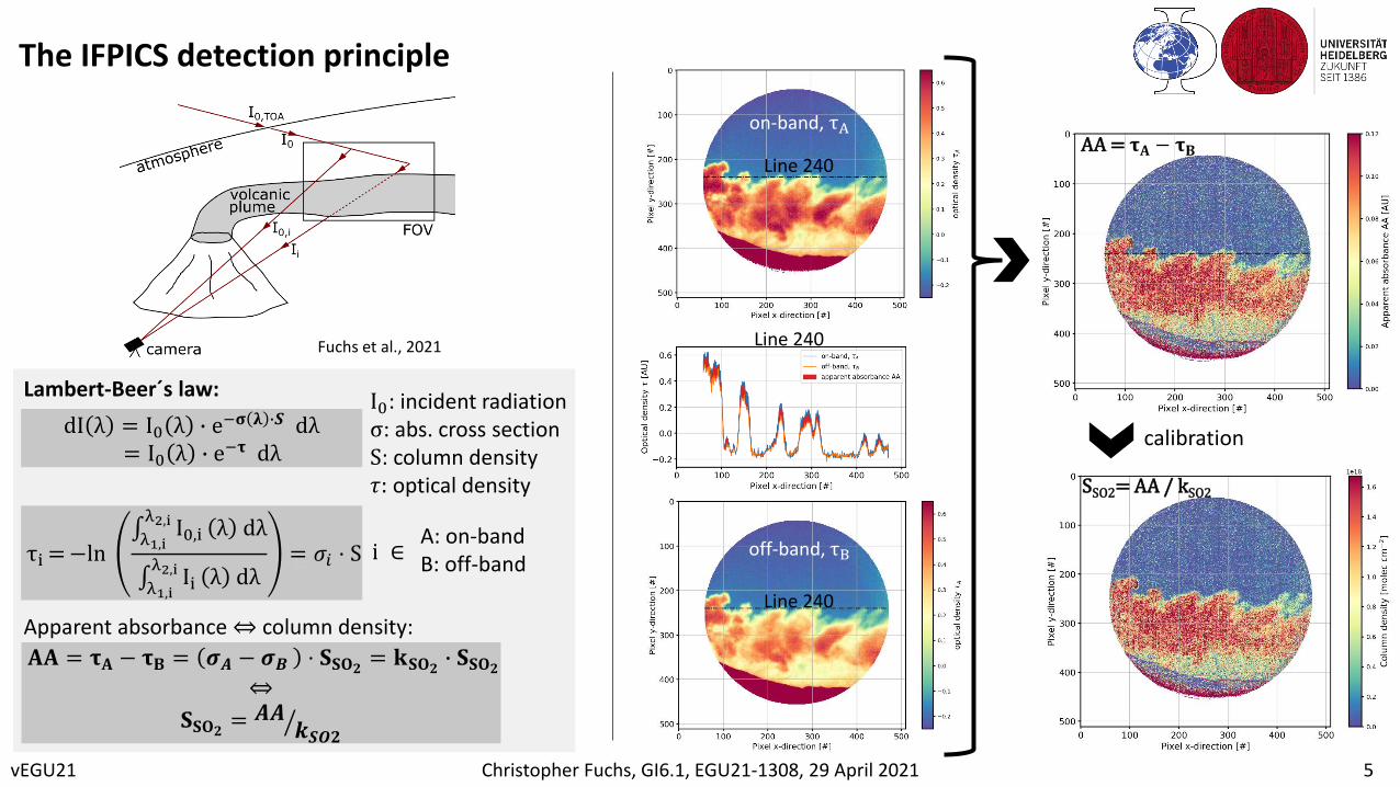
The IFPICS detection principle

dI λ = I0 λ ∙ e−𝛔 𝛌 ∙𝑺 dλ= I0 λ ∙ e−𝛕 dλ

τi=−lnλ1,iλ2,i I0,i λ dλ

λ1,iλ2,i Ii λ dλ

= 𝜎𝑖 ⋅ S

𝐀𝐀 = 𝛕𝐀 − 𝛕𝐁 = 𝝈𝑨 − 𝝈𝑩 ⋅ 𝐒𝐒𝐎𝟐 = 𝐤𝐒𝐎𝟐 ∙ 𝐒𝐒𝐎𝟐⇔

𝐒𝐒𝐎𝟐 = ൗ𝑨𝑨𝒌𝑺𝑶𝟐

Lambert-Beer´s law: I0: incident radiationσ: abs. cross sectionS: column density𝜏: optical density

A: on-bandB: off-band

i ∈

Apparent absorbance ⇔ column density:

on-band, τA

off-band, τB

Line 240

Line 240

Line 240

AA = 𝛕𝐀 − 𝛕𝐁

calibration

SSO2= AA / kSO2

Fuchs et al., 2021


The calibration of IFPICS data

For the calibration of the recorded data apparent absorbance AA into column densities CD a forward instrument model is used.

The model is based on high resolution solar atlas spectrum and literature absorption cross sections.

Thereby the model includes:• potentially interfering trace gas species• the divergence of the light beams inside the instrument • optical losses due to imperfect optics• UV detector characteristics and quantum efficiency• Inherent including saturation effects due to high gas concentrations

Model calculations:Divergence of the light beam results in a decrease of the FPIs effective Finesse (damping the peaks of max. FPI transmission)

Consistency check of the forward instrument model by a conventional calibration based on SO2 gas cells:Measurement of 3 SO2 gas cells using:1. IFPICS instrument for apparent absorbance AA values2. DOAS system to retrieve SO2 column densities (CD)

➔ Instrument model represents measured data within rangeof uncertainties.

➔ A polynomial function AA(CDSO2) is fitted to the model. The inversion of the polynomial is used to calibrate AA into CD by CDSO2(AA) = [ AA(CDSO2) ]-1

Fuchs et al., 2021


Camera performance & measurement setup at Mt. Etna, 02 October 2020

Google Earth ©; Gorelick, N., et al.

FOV

• Location: 37°42‘ N, 15°01‘ W, ”Schiena del Asino“, ≈ 2000 m A.S.L

• Spatial resolution & pixel size: 400x400 pix with 3.8m x 3.8m size

• Temporal resolution: 3.28 s

• Detection limit: 2.61+1017 molec cm-2 s-1/2

• Camera viewing direction: 357°N, 18° Elevation

• Camera field of view (FOV): 18°

• Plume & wind direction: 45° W

• Windspeed: ≈ 10.8 m/s (UWYO; atmo. soundings)

• Plume distance: ≈ 4700 m

Etnacrater

vEGU21 Christopher Fuchs, GI6.1, EGU21-1308, 29 April 2021

Results: 1.) Plume (wind) velocity retrieval from imaging data

Plume propagation velocity data can be retrieved directly from imaging data using optical-flow algorithms the cross-correlation approach.

Cross-correlation: 1. Integrate recorded signal (AA, or CD) along different columns

perpendicular to the observed plume propagation direction (i.e.: col. 1: row 250, col. 2: row 300, col. 3: row 350, col. 4: row 400).

2. Find max correlation by shifting signal over time (images) with respect to certain column (i.e. with respect to column 1)

3. Max correlation determines time required for plume to travel certain pixel → allows to retrieve velocity using pixel size

Results:

• Col 1-2: lag of 5 images = 16.4s, 50 pix = 190m, correlation 87%• Col 1-3: lag of 10 images = 32.8s, 100 pix = 380m, correlation 77%• Col 1-4: lag of 15 images = 49.2s, 150 pix = 570m, correlation 66%

➔ Plume propagation velocity: 11.58 m/s (wind data: ≈ 10.8 m/s) (http://weather.uwyo.edu/upperair/sounding.html)

Column:1 2 3 4

Google Earth ©; Gorelick, N., et al.

1

2

1

34

234

8

http://weather.uwyo.edu/upperair/sounding.html


Results: 2.) SO2 mass fluxes from imaging data

9

The volcanic SO2 mass flux Φ𝑆𝑂2 can be determined directly from

calibrated imaging data by:

Integration along a plume transect of length L of the evaluated SO2 CD image series ℎ𝑝𝑖𝑥 ⋅ 𝐶𝐷𝑆𝑂2 𝑑𝐿. A subsequent multiplication with the

perpendicular wind velocity 𝑣⊥𝑤𝑖𝑛𝑑 then yielding the SO2 flux through

the plume transect.As the pixel of the detector are discrete (finite size) the integration is replaced by summation:

We retrieved SO2 mass fluxes of:

𝚽𝑺𝑶𝟐 = (726 ± 130) t/day

Preliminary results!

Φ𝑆𝑂2 = නℎ𝑝𝑖𝑥 ⋅ 𝐶𝐷𝑆𝑂2 𝑑𝐿 ⋅ 𝑣⊥𝑤𝑖𝑛𝑑 =

𝑖

ℎ𝑝𝑖𝑥𝑖 ⋅ 𝐶𝐷𝑆𝑂2,𝑖 ⋅ 𝑣⊥𝑤𝑖𝑛𝑑

L


Conclusion & Outlook

10

Conclusion:• First successful application of the new technique IFPICS• The instrument is robust and small hence applicable even

under harsh environmental conditions• Good sensitivity and low cross-interferences• Calibration is based on a forward model making infield

calibration redundant

Outlook: • Revising instrument (already done) and perform new

measurements with improved 2D UV detector• Field measurements of weaker SO2 emitter• Extension of the IFPICS technique to further trace gases,

e.g., BrO, HCHO, NO2

➔Have a look at EGU contribution: EGU21-2811, A. Nies et al., IFPICS measurements of HCHOLink: https://meetingorganizer.copernicus.org/EGU21/EGU21-2811.html

Thank you for [email protected]

https://meetingorganizer.copernicus.org/EGU21/EGU21-2811.html


References:

11

• Louban et al., 2009: Louban, I., Bobrowski, N., Rouwet, D. et al. Imaging DOAS for volcanological applications. Bull Volcanol 71, 753–765 (2009). https://doi.org/10.1007/s00445-008-0262-6

• Lübcke et al., 2013: Lübcke, P., Bobrowski, N., Illing, S., Kern, C., Alvarez Nieves, J. M., Vogel, L., Zielcke, J., Delgado Granados, H., and Platt, U.: On the absolute calibration of SO2 cameras, Atmos. Meas. Tech., 6, 677–696, https://doi.org/10.5194/amt-6-677-2013, 2013.

• Fuchs et al., 2021: Fuchs, C., Kuhn, J., Bobrowski, N., and Platt, U.: Quantitative imaging of volcanic SO2 plumes using Fabry–Pérot interferometer correlation spectroscopy, Atmos. Meas. Tech., 14, 295–307, https://doi.org/10.5194/amt-14-295-2021, 2021.

• UWYO: University of Wyoming, Department of Atmopsheric Science, atmospheric soundings; Station data: Trapani (LICT), Italy 2019-07-22 12:00, available at: http://weather.uwyo.edu/upperair/sounding.html, last access: April 2021.

• Google Earth ©; Gorelick, N., et al.: Gorelick, N., Hancher, M., Dixon, M., Ilyushchenko, S., Thau, D., & Moore, R. (2017). Google Earth Engine: Planetary-scale geospatial analysis for everyone. Remote Sensing of Environment. Accessed: April 2021

https://doi.org/10.1007/s00445-008-0262-6

https://doi.org/10.5194/amt-6-677-2013

https://doi.org/10.5194/amt-14-295-2021

http://weather.uwyo.edu/upperair/sounding.html

Technological advances to improve the quantification of ...

Documents

Transcript of Technological advances to improve the quantification of ...