
Techniques for Multi-Standard Cognitive Radios on FPGAs · PDF fileThe thesis explores...
194
NANYANG TECHNOLOGICAL UNIVERSITY Techniques for Multi-Standard Cognitive Radios on FPGAs Pham Hung Thinh School of Computer Engineering A thesis submitted to Nanyang Technological University in partial fulfilment of the requirements for the degree of Doctor of Philosophy September 2015
Transcript of Techniques for Multi-Standard Cognitive Radios on FPGAs · PDF fileThe thesis explores...

NANYANG TECHNOLOGICAL UNIVERSITY
Techniques for Multi-Standard
Cognitive Radios on FPGAs
Pham Hung Thinh
School of Computer Engineering
A thesis submitted to Nanyang Technological University
in partial fulfilment of the requirements for the degree of
Doctor of Philosophy
September 2015

Acknowledgments
It is great pleasure to me in expressing my gratitude to all those people who
have continuously supported me and had their contributions in making this thesis
possible.
I would like to express my sincere thanks and appreciation to my supervisors, Prof.
Suhaib Fahmy, and Prof. Ian McLoughlin for giving me constant trust during the
entire research of my Ph.D. studies, for their helpful suggestions and advices, for
their continuous support and their teachings essential to achieve this objective.
I express my sincere gratitude towards Prof. Samarjit Chakraborty at Institute
for Real-Time Computer Systems, TU Munich for providing me an internship
opportunity in the final stage of my PhD.
I also wish to thank all colleagues and technical staffs in CHiPES for their prompt
support and helpful in providing all the facilities required for my research work.
Last but not least, I would like to acknowledge my family in Viet Nam, for their
constant love and encouragement.
i

Abstract
The thesis explores techniques for enabling cognitive radio design on field pro-
grammable gate arrays (FPGAs). We demonstrate the strengths of FPGAs in
offering a high throughput, low-power baseband platform, and develop a flexi-
ble Orthogonal Frequency Division Multiplexing (OFDM) baseband chain with
high-level control and support for multiple standards. We present contributions
in OFDM synchronisation to enable more robust radios in harsher channels, and
tolerating less precise RF components. We also present a novel technique for
managing out of band leakage to enable more efficient spectral use in a dynamic
spectrum allocation setting. For each of these approaches, we design, optimise,
and characterise working hardware implementations of the required modules, with
a focus on flexibility and low power. Finally, we present an approach for apply-
ing FPGA partial reconfiguration to minimise reconfiguration time when a radio
switches modes, allowing intermediate data to be buffered and processed after re-
configuration is complete. These contributions form an important foundation in
building a fully functional prototyping platform for cognitive radio systems.
ii

Contents
Acknowledgments . . . . . . . . . . . . . . . . . . . . . . . . . . . . . i
Abstract . . . . . . . . . . . . . . . . . . . . . . . . . . . . . . . . . . . ii
List of Abbrevations xi
List of Notation . . . . . . . . . . . . . . . . . . . . . . . . . . . . . . xiv
1 Introduction 1
1.1 Motivation . . . . . . . . . . . . . . . . . . . . . . . . . . . . . . . . 3
1.2 Objectives . . . . . . . . . . . . . . . . . . . . . . . . . . . . . . . . 4
1.3 Research Contributions . . . . . . . . . . . . . . . . . . . . . . . . . 5
1.4 Organisation . . . . . . . . . . . . . . . . . . . . . . . . . . . . . . . 7
1.5 Publications . . . . . . . . . . . . . . . . . . . . . . . . . . . . . . . 8
2 Background Literature 10
2.1 Cognitive and Software Defined Radio . . . . . . . . . . . . . . . . 10
2.1.1 Multi-Standard Cognitive Radios . . . . . . . . . . . . . . . 12
2.1.2 Existing Radio Platforms . . . . . . . . . . . . . . . . . . . . 15
2.2 Orthogonal Frequency Division Multiplexing . . . . . . . . . . . . . 17
2.2.1 Cyclic Prefix . . . . . . . . . . . . . . . . . . . . . . . . . . 18
2.2.2 OFDM Radio Systems . . . . . . . . . . . . . . . . . . . . . 20
2.2.3 Evaluating OFDM . . . . . . . . . . . . . . . . . . . . . . . 23
2.2.4 OFDM Synchronisation . . . . . . . . . . . . . . . . . . . . 24
2.2.4.1 Timing Offsets . . . . . . . . . . . . . . . . . . . . 24
2.2.4.2 Frequency Offset . . . . . . . . . . . . . . . . . . . 27
2.2.4.3 Phase Noise . . . . . . . . . . . . . . . . . . . . . . 30
2.2.5 Shaping OFDM Spectral Leakage . . . . . . . . . . . . . . . 31
2.2.5.1 Spectrum Emission Masks in Recent Standards . . 31
2.2.5.2 Dynamic Channel Requirements . . . . . . . . . . 33
2.2.5.3 Filtering in OFDM Implementations . . . . . . . . 34
2.3 Field Programmable Gate Arrays . . . . . . . . . . . . . . . . . . . 36
2.3.1 FPGAs for Radio Platforms . . . . . . . . . . . . . . . . . . 36
2.3.2 Power Dissipation on FPGA . . . . . . . . . . . . . . . . . . 37
2.3.3 Power Estimation Tools . . . . . . . . . . . . . . . . . . . . 41
2.4 Summary . . . . . . . . . . . . . . . . . . . . . . . . . . . . . . . . 43
iii

CONTENTS iv
3 Multiplierless Correlator Design for OFDM Timing Synchronisa-tion 44
3.1 Introduction . . . . . . . . . . . . . . . . . . . . . . . . . . . . . . . 44
3.2 Implementing Correlators . . . . . . . . . . . . . . . . . . . . . . . 46
3.2.1 Design of DSP48E1 Based Correlator . . . . . . . . . . . . . 47
3.2.2 Design of Multiplierless Correlator . . . . . . . . . . . . . . 49
3.2.3 Implementation Results . . . . . . . . . . . . . . . . . . . . 50
3.3 Simulation and Discussion . . . . . . . . . . . . . . . . . . . . . . . 53
3.4 Summary . . . . . . . . . . . . . . . . . . . . . . . . . . . . . . . . 55
4 Method for OFDM Timing Synchronisation 56
4.1 Introduction . . . . . . . . . . . . . . . . . . . . . . . . . . . . . . . 56
4.2 Related Work . . . . . . . . . . . . . . . . . . . . . . . . . . . . . . 57
4.2.1 Coarse STO and Fractional CFO Estimation . . . . . . . . . 58
4.2.2 Fractional CFO Compensation . . . . . . . . . . . . . . . . . 60
4.2.3 Fine STO Estimation . . . . . . . . . . . . . . . . . . . . . . 61
4.3 Proposed Fractional CFO Estimation and Synchronisation . . . . . 62
4.3.1 Frame Synchronisation and Fractional CFO Estimation . . . 66
4.3.2 Fractional CFO Compensation . . . . . . . . . . . . . . . . . 68
4.3.3 Simulation Results and Discussion . . . . . . . . . . . . . . . 68
4.3.3.1 Performance in AWGN . . . . . . . . . . . . . . . . 69
4.3.3.2 Performance in Fading Channels . . . . . . . . . . 71
4.3.3.3 Performance with Large Frequency Offset . . . . . 72
4.3.4 Hardware Implementation . . . . . . . . . . . . . . . . . . . 73
4.3.4.1 Implementation of Conventional Synchroniser . . . 74
4.3.4.2 Implementation of Proposed Synchroniser . . . . . 75
4.3.4.3 Effect of Reduced Precision . . . . . . . . . . . . . 77
4.3.4.4 Optimized Alternatives . . . . . . . . . . . . . . . 80
4.4 Summary . . . . . . . . . . . . . . . . . . . . . . . . . . . . . . . . 82
5 IFO Estimation Method for OFDM Frequency Synchronisation 83
5.1 Introduction . . . . . . . . . . . . . . . . . . . . . . . . . . . . . . . 83
5.2 Related Work . . . . . . . . . . . . . . . . . . . . . . . . . . . . . . 84
5.3 Enhanced OFDM Synchronisation Through Novel IFO EstimationArchitecture . . . . . . . . . . . . . . . . . . . . . . . . . . . . . . . 87
5.3.1 Proposed Algorithm . . . . . . . . . . . . . . . . . . . . . . 88
5.3.2 Proposed Architecture . . . . . . . . . . . . . . . . . . . . . 89
5.3.3 Simulation . . . . . . . . . . . . . . . . . . . . . . . . . . . . 93
5.3.3.1 Performance Comparison . . . . . . . . . . . . . . 95
5.3.3.2 Wordlength Optimisation . . . . . . . . . . . . . . 98
5.3.4 FPGA Implementation . . . . . . . . . . . . . . . . . . . . . 101
5.3.4.1 Conventional Approach . . . . . . . . . . . . . . . 101
5.3.4.2 Proposed Approach . . . . . . . . . . . . . . . . . . 102
5.3.5 Implementation Results . . . . . . . . . . . . . . . . . . . . 103
5.4 Summary . . . . . . . . . . . . . . . . . . . . . . . . . . . . . . . . 105

CONTENTS v
6 Spectrum Efficient Shaping Method for OFDM Cognitive Radios106
6.1 Introduction . . . . . . . . . . . . . . . . . . . . . . . . . . . . . . . 106
6.2 Signal Model for Spectral Leakage Filtering . . . . . . . . . . . . . 107
6.2.1 Signal Model . . . . . . . . . . . . . . . . . . . . . . . . . . 108
6.2.2 802.11p Signal and Channel Models . . . . . . . . . . . . . . 109
6.2.3 802.11af Signal and Channel Models . . . . . . . . . . . . . 110
6.3 Related Work . . . . . . . . . . . . . . . . . . . . . . . . . . . . . . 110
6.3.1 Pulse Shaping . . . . . . . . . . . . . . . . . . . . . . . . . . 111
6.3.2 Image Spectrum Cancellation By FIR Filter . . . . . . . . . 115
6.4 Proposed Spectrum Efficient Shaping Method . . . . . . . . . . . . 118
6.4.1 New Spectral Leakage Filtering Method . . . . . . . . . . . 118
6.4.2 Novel CR Filtering Architecture . . . . . . . . . . . . . . . . 120
6.5 Simulation Results and Discussion . . . . . . . . . . . . . . . . . . . 123
6.5.1 Configuration and Performance Evaluation for 802.11p . . . 123
6.5.2 Configuration and Performance Evaluation for 802.11af . . . 126
6.5.3 802.11af Spectral Efficiency . . . . . . . . . . . . . . . . . . 127
6.6 Summary . . . . . . . . . . . . . . . . . . . . . . . . . . . . . . . . 129
7 An Architecture for Multi-Standard Cognitive Radios 131
7.1 Introduction . . . . . . . . . . . . . . . . . . . . . . . . . . . . . . . 131
7.2 Related Work . . . . . . . . . . . . . . . . . . . . . . . . . . . . . . 132
7.3 Proposed OFDM Baseband for MSCR . . . . . . . . . . . . . . . . 134
7.3.1 System Description . . . . . . . . . . . . . . . . . . . . . . . 134
7.3.2 Module Description . . . . . . . . . . . . . . . . . . . . . . . 138
7.3.2.1 FIFO Buffer (FIFO) . . . . . . . . . . . . . . . . . 138
7.3.2.2 Synchronisation (Synch) . . . . . . . . . . . . . . . 139
7.3.2.3 Frequency Compensation . . . . . . . . . . . . . . 140
7.3.2.4 Fine STO Estimation . . . . . . . . . . . . . . . . 141
7.3.2.5 Remove Cyclic Prefix . . . . . . . . . . . . . . . . . 142
7.3.2.6 FFT . . . . . . . . . . . . . . . . . . . . . . . . . . 143
7.3.2.7 IFO Estimation and Channel Equalisation . . . . . 143
7.3.2.8 Phase Tracking . . . . . . . . . . . . . . . . . . . . 144
7.3.2.9 Data symbol demodulation (DatSymDem) . . . . . 146
7.4 Performance Analysis and Discussion . . . . . . . . . . . . . . . . . 146
7.4.1 Latency and Stalling for PR-Based Baseband . . . . . . . . 146
7.4.2 Analysing the Proposed OFDM MSCR Approach . . . . . . 150
7.5 System Verification . . . . . . . . . . . . . . . . . . . . . . . . . . . 156
7.6 Summary . . . . . . . . . . . . . . . . . . . . . . . . . . . . . . . . 159
8 Conclusions and Future Work 161
8.1 Summary of Contributions . . . . . . . . . . . . . . . . . . . . . . . 161
8.1.1 Robust, Efficient Synchronisation . . . . . . . . . . . . . . . 162
8.1.2 OFDM Spectrum Shaping . . . . . . . . . . . . . . . . . . . 162
8.1.3 Multi-Standard Radio Design . . . . . . . . . . . . . . . . . 163

CONTENTS vi
8.2 Future Research Directions . . . . . . . . . . . . . . . . . . . . . . . 163
8.2.1 Increasing Spectrum Efficiency with Shaping for NC-OFDM 163
8.2.2 Efficiently Adaptive Shaping Spectral Leakage . . . . . . . . 164
8.2.3 Standardised Software Interface for Multi-Standard RadioPlatform . . . . . . . . . . . . . . . . . . . . . . . . . . . . . 164
8.2.4 Alternative MultiCarrier Modulations Techniques . . . . . . 164
8.2.5 Higher Layer Knowledge to Minimise Reconfiguration Time 165
8.3 Summary . . . . . . . . . . . . . . . . . . . . . . . . . . . . . . . . 165
Bibliography 166

List of Figures
2.1 Block diagram of a multicarrier modulated system, (a) in the countinuous-time and (b) in discrete-time . . . . . . . . . . . . . . . . . . . . . . 13
2.2 The spectrum of subcarriers in OFDM [1]. . . . . . . . . . . . . . . 17
2.3 OFDM transmission without cyclic prefix results in ISI among ad-jacent symbol. . . . . . . . . . . . . . . . . . . . . . . . . . . . . . . 19
2.4 OFDM transmission with cyclic prefix avoids ISI among adjacentsymbol. . . . . . . . . . . . . . . . . . . . . . . . . . . . . . . . . . 20
2.5 Inserting Cyclic Prefix in the OFDM symbol. . . . . . . . . . . . . 20
2.6 An OFDM system model. . . . . . . . . . . . . . . . . . . . . . . . 20
2.7 Block diagram of an OFDM radio system. . . . . . . . . . . . . . . 22
2.8 OFDM received symbol with timing offsets of -1, 1, -5 and 5 in a,b, c, d, respectively. . . . . . . . . . . . . . . . . . . . . . . . . . . . 26
2.9 Inter carrier interference (ICI) caused by frequency offset ∆f . . . . 27
2.10 The constellations of OFDM received symbol with frequency offetsof 0.025, 0.5, 0.1 and 0.25 sub-carries spacing in a, b, c, d, respectively. 29
2.11 The constellations of 5 consecutive OFDM received symbols withfrequency offsets of 0.025 and 0.05 in a, b respectively. . . . . . . . 29
2.12 The constellations of an OFDM received symbol and 5 consecutiveOFDM received symbols with phase noise variance of 0.25 rad2 in(a), (b) respectively. . . . . . . . . . . . . . . . . . . . . . . . . . . 30
2.13 The comparison between TVBD SEM and 802.11 scaled SEM. . . . 32
2.14 The comparison between traditional and DUC Front-end. . . . . . . 35
3.1 Downlink preamble symbols for IEEE 802.16. . . . . . . . . . . . . 46
3.2 Transposed direct form correlator. . . . . . . . . . . . . . . . . . . . 46
3.3 Structure of DSP48E1 block inside the Virtex-6 [2]. . . . . . . . . . 48
3.4 Pipeline structure of the complex number multiply-add. . . . . . . . 48
3.5 Pipeline structure of correlator using DSP48E1 blocks. . . . . . . . 48
3.6 Structure of multiplierless correlators. . . . . . . . . . . . . . . . . . 49
3.7 Correlator power consumption at different frequencies. . . . . . . . 53
3.8 Correlator output with SNR = 10 dB. . . . . . . . . . . . . . . . . . 54
3.9 Detection failure rate with increasing SNR. . . . . . . . . . . . . . . 55
4.1 The timing metric in [3] applied to the IEEE 802.16-2009 preamblein an AWGN channel (SNR = 10dB) . . . . . . . . . . . . . . . . . 58
vii

LIST OF FIGURES viii
4.2 The timing metric in [4] applied to the IEEE 802.16 preamble in anAWGN channel (SNR = 10dB) . . . . . . . . . . . . . . . . . . . . 63
4.3 Proposed timing metrics applied to the IEEE 802.16 preamble inAWGN (SNR = 10 dB, CFO = 10.5). . . . . . . . . . . . . . . . . . 64
4.4 The synchronisation flow according to the received samples withinthe preamble showing its packet format above the conventional syn-chronisation scheme flow (middle), and proposed scheme (bottom).With the packet timing illustrated above. . . . . . . . . . . . . . . . 65
4.5 Performance of the frame synchronisation method versus the selec-tion threshold for an AWGN channel (with SNR =10dB). . . . . . . 66
4.6 Performance of time synchronisation in AWGN channels with a fre-quency offset of 0.5 subcarrier spacings. . . . . . . . . . . . . . . . . 70
4.7 Performance of fractional frequency offset estimation in AWGNchannels. . . . . . . . . . . . . . . . . . . . . . . . . . . . . . . . . . 70
4.8 Frame synchronisation performance of various methods in an SUI1channel with respect to SNR. . . . . . . . . . . . . . . . . . . . . . 71
4.9 Frame synchronisation performance of various methods in an SUI2channel with respect to SNR. . . . . . . . . . . . . . . . . . . . . . 72
4.10 Performance of frame synchronisation in an AWGN channel withuniform random frequency offset varying from -10 to 10 times carrierspacing, with respect to SNR. . . . . . . . . . . . . . . . . . . . . . 73
4.11 Architecture of the conventional synchronisation FPGA implemen-tation. . . . . . . . . . . . . . . . . . . . . . . . . . . . . . . . . . . 74
4.12 Architecture for the proposed synchronisation method implementedon FPGA. . . . . . . . . . . . . . . . . . . . . . . . . . . . . . . . . 75
4.13 Implementation of energy correlator on FPGA. . . . . . . . . . . . 77
4.14 Performance of CFO estimation in an AWGN channel against SNR,with different numbers of fractional bits used in the computation ofP ′. . . . . . . . . . . . . . . . . . . . . . . . . . . . . . . . . . . . . 78
4.15 Performance of frame synchronisation in an AWGN channel againstSNR, with different numbers of fractional bits used in the compu-tation of R′. . . . . . . . . . . . . . . . . . . . . . . . . . . . . . . . 79
5.1 Baseband processing block diagram. . . . . . . . . . . . . . . . . . . 84
5.2 Pilots in the long preamble of IEEE 802.16-2009. . . . . . . . . . . 87
5.3 Circuit for the known-pilots shift register. . . . . . . . . . . . . . . 90
5.4 Resource sharing approach for computing Vε. . . . . . . . . . . . . . 91
5.5 Architecture of proposed IFO estimator. . . . . . . . . . . . . . . . 92
5.6 Fail rate of IFO estimation methods in AWGN channel without RTO. 96
5.7 Fail rate of IFO estimation methods in AWGN channel with RTO. . 96
5.8 Fail rate of IFO estimation methods in SUI1 channel. . . . . . . . . 97
5.9 Fail rate of IFO estimation methods in SUI2 channel. . . . . . . . . 97
5.10 Fail rate for different wordlengths in AWGN channel without RTO. 99
5.11 Fail rate for different wordlengths in AWGN channel with RTO. . . 99
5.12 Fail rate for different wordlengths in SUI1 channel. . . . . . . . . . 100

LIST OF FIGURES ix
5.13 Fail rate for different wordlengths in SUI2 channel. . . . . . . . . . 100
5.14 DSP block based 3-input adder for correlation. . . . . . . . . . . . . 102
6.1 Pulse Shaping operation performed on OFDM symbols. . . . . . . . 113
6.2 Spectral envelope due to pulse shaping OFDM symbols using threesmoothing functions and different roll-off factors for 802.11p. ClassC and D spectral emission mask limits are overlaid as dotted lines. . 113
6.3 Spectrum of 802.11p OFDM symbols shaped with different windowfunctions, with the image spectrum included. . . . . . . . . . . . . . 114
6.4 Spectra of OFDM symbols for 802.11p using different FIR interpo-lation filters, with L = 8. . . . . . . . . . . . . . . . . . . . . . . . . 117
6.5 The CR-Based architecture for adaptive OFDM spectral leakageshaping. . . . . . . . . . . . . . . . . . . . . . . . . . . . . . . . . . 120
6.6 Spectrum of 802.11p signal of the proposed CR architecture afterinterpolation. . . . . . . . . . . . . . . . . . . . . . . . . . . . . . . 124
6.7 Spectrum of 802.11p signal using option Prop1 with 20th order FIRfiltering. . . . . . . . . . . . . . . . . . . . . . . . . . . . . . . . . . 125
6.8 Spectrum of 802.11p signal for Prop2 with 12th order FIR filtering. 125
6.9 Spectrum of 802.11af signal using the proposed CR architecture. . . 127
6.10 Fitting Filtered Spectrum of 802.11af signal to SEMs. . . . . . . . . 129
7.1 The structure of a generic MSCR system . . . . . . . . . . . . . . . 134
7.2 The receiver FIFO module. . . . . . . . . . . . . . . . . . . . . . . . 139
7.3 Block diagram of Synchronisation module. . . . . . . . . . . . . . . 140
7.4 Block diagram of frequency compensation module. . . . . . . . . . . 141
7.5 Block diagram of fine STO estimation module. . . . . . . . . . . . . 142
7.6 The block diagram of IFO estimation and channel equalisation . . . 144
7.7 Block diagram of phase tracking module. . . . . . . . . . . . . . . . 146
7.8 Comparison of reconfiguration latency for a single and multiple PRmodules. . . . . . . . . . . . . . . . . . . . . . . . . . . . . . . . . . 147
7.9 Bitstream sizes for PR modules. . . . . . . . . . . . . . . . . . . . . 152
7.10 The latency of sub-modules for three standards . . . . . . . . . . . 152
7.11 The configuration time and latency of sub-modules for OFDM-based MSCR system . . . . . . . . . . . . . . . . . . . . . . . . . . 153
7.12 A scenario of a transmission . . . . . . . . . . . . . . . . . . . . . . 154
7.13 The halting time comparison of the system for three different ap-proaches. . . . . . . . . . . . . . . . . . . . . . . . . . . . . . . . . . 154
7.14 A comparison of the three approaches in terms of system reconfig-uration latency and FIFO requirements. . . . . . . . . . . . . . . . 155
7.15 Verification framework. . . . . . . . . . . . . . . . . . . . . . . . . . 156
7.16 Block diagram of verified system . . . . . . . . . . . . . . . . . . . . 157
7.17 The verification results of the transmitter. . . . . . . . . . . . . . . 158
7.18 Verification results of the receiver. . . . . . . . . . . . . . . . . . . . 158
7.19 Verification results of the baseband system. . . . . . . . . . . . . . . 159

List of Tables
3.1 Resource utilisation summary. . . . . . . . . . . . . . . . . . . . . . 50
3.2 Correlator power consumption at 50 MHz. . . . . . . . . . . . . . . 52
4.1 Resources required for computing P ′ on FPGA with different wordlengths, Q1.f1. . . . . . . . . . . . . . . . . . . . . . . . . . . . . . 78
4.2 Resources required for computing R’ on FPGA with different wordlengths, Q1.f2. . . . . . . . . . . . . . . . . . . . . . . . . . . . . . 79
4.3 Total resources consumed by a full word length implementation ofSoA and four reduced complexity instances of the proposed method.Dynamic (Dpwr) and quiescent power (Qpwr) consumption are re-ported in mA. Maximum frequency is reported in MHz. . . . . . . . 80
4.4 Resource comparison between two synchronisation methods. . . . . 81
5.1 Resource utilisation and dynamic power of IFO estimators. . . . . . 103
6.1 Major parameters of 802.11p and 802.11af OFDM PHYs . . . . . . 109
6.2 Popular window-based FIR filter lengths . . . . . . . . . . . . . . . 116
6.3 Hardware Usage for spectral shaping . . . . . . . . . . . . . . . . . 122
7.1 System specifications of three supported OFDM-based standards. . 135
7.2 Parameterised values according to supported standards . . . . . . . 140
7.3 Allocation vector coding. . . . . . . . . . . . . . . . . . . . . . . . . 145
7.4 Resources for 802.22 OFDM-based implementation . . . . . . . . . 151
7.5 Memory resources for 32 bit AXI4 interface FIFOs implementation 155
x

List of Abbrevations
ADC Analogue to Digital Converter
ASICs Application Specific Integrated Circuits
AWGN Additive White Gaussian Noise
AXI Advanced eXtensible Interface
BCU Basic Channel Unit
BER Bit Error Rate
BPSK Binary Phase Shift Keying
CFO Carrier Frequency Offset
CIR Channel Impulse Response
COTS Commercial Off-The-Shelf
CP Cyclic Prefix
CPE Common Phase Error
CR Cognitive Radio
DAC Digital to Analogue Converter
DFT Discrete Fourier Transform
DMT Discrete Multi Tone
DSA Dynamic Spectrum Access
DSP Digital Signal Processing
DSRC Dedicated Short-Range Communications
xi

LIST OF ABBREVATIONS xii
FBMC Filter Bank Multi-Carrier
FDM Frequency Division Multiplexing
FFO Fractional Frequency Offset
FFT Fast Fourier Transform
FPGA Field Programmable Gate Array
ICAP Internal Configuration Access Port
ICI Inter Carrier Interference
IDFT Inverse Discrete Fourier Transform
IFFT Inverse Fast Fourier Transform
IFO Integer Frequency Offset
IQ In-phase - Quadrature
ISI Inter Symbol Interference
IUs Incumbent Users
LNA Low Noise Amplifier
MAN Metropolitan Area Networks
MCM Multi-Carrier Modulation
MIMO Multi-Input Multi-Output
ML Maximum Likelihood
MPoC Multiple Processors on Chip
MSB Most Significant Bit
MSCRs Multiple Standard Cognitive Radios
MSE Mean Squared Error
NC-OFDM Non-Contiguous Orthogonal Frequency Division Multiplexing
OFDM Orthogonal Frequency Division Multiplexing
PAPR Peak-to-Average Power Ratio

LIST OF ABBREVATIONS xiii
PAR Place And Route
PDF Probability Density Function
PLL Phase-Locked Loop
PR Partial Reconfiguration
PUs Primary Users
QAM Quadrature Amplitude Modulation
QPSK Quadrature Phase Shift Keying
RF Radio Frequency
RTL Register Transfer Level
RTO Residual Timing Offset
RTV Road to Vehicle
SEM Spectrum Emission Mask
SER Symbol Error Rate
SNR Signal to Noise Ratio
STO Symbol Timing Offset
SUI Stanford University Interim
SUs Secondary Users
TVBD TV Band Devices
TVWS Television White Spaces
V2V Vehicle-to-Vehicle
WLAN Wireless Local Area Networks
XPA Xilinx Power Analyzer
XPE Xilinx Power Estimator

List of Notation
∗ Convolution
(·)T Matrix or vector transpose
i imaginary unit
|a| absolute value of the number a
∠a argument of a complex number in [0, 2π]
a compensated for the parameter a
x(t) time continuous signal
x[d] time discrete signal; d is time index
x[d]′ offseted discrete signal
x[d] compensated discreate signal
∆fC carrier frequency offset normalized to the intercarrier spacing
sinc(t) , sin(πt)(πt)
(f ∗ g)(m) ,∑
n f(n)g(m− n) convolution product
xiv

Chapter 1
Introduction
Wireless transmission plays a key role in our everyday lives, and has enabled
the exponential growth in connectivity that we have witnessed over the last few
decades. An exponential increase in the number of users and nodes, and the
throughput demanded between them, means significant developments are crucial
in the fundamental methods by which this wireless communication is enabled. The
previous approach of defining fixed wireless standards for use in fixed portions of
radio spectrum is giving way to a more dynamic approach to exploiting this scarce
resource. Practical studies have shown that many licensed bands are relatively
unused across time and frequency [5]. To improve the efficiency of radio spectrum
use, the concept of unlicensed users temporarily reusing unused spectrum in li-
censed bands is currently being researched. This concept is known as dynamic
spectrum access (DSA) [6]. Wireless communication systems for realising DSA
must be reconfigurable, to support different radio standards in different environ-
ments, and adaptive, to react to changing channel conditions without interfering
with licensed users and other unlicensed opportunistic users.
A cognitive radio (CR) is a node that is able to adapt its parameters to optimise
performance based on interaction with the environment, as well as to perform
DSA. A cognitive radio can modify parameters such as transmit power, coding
rate, frame size, bandwidth, and centre frequency, in real time, to obtain suit-
able performance in a changing, environment. The radio baseband should also be
1

Chapter 1 Introduction 2
reconfigurable to enable support for multiples standards such as WiFi, WiMAX,
GSM, WCDMA, and other defined access schemes. More advanced adaptive stan-
dards are intrinsically flexible and this flexibility should be managed to optimise
performance in the channel.
This thesis explores techniques for enabling the mapping and implementation of
dynamic cognitive radios on FPGA platforms. By dynamic, we are referring to
the ability to modify baseband processing to suit difference transmission standards
and scenarios. The decision making and spectral sensing aspects of cognitive radio
are not addressed in this thesis. In the context of our work, we are interested in
providing a generalised interface for cognitive radio designers to be able to leverage
the dynamic capabilities of the hardware platform at a higher level. By general-
ising the interface, we allow arbitrarily complex cognitive engines to leverage the
flexibility of the baseband
FPGAs are silicon devices that allow us to build customised hardware datapaths
for a variety of applications. By exploiting parellelism inherent in many algo-
rithms, it is possible to develop implementations that are significantly faster than
equivalent software running on general purpose processors. FPGAs have long
been established as a platform of choice in signal processing due to their suitabil-
ity for parallel bit-level architectures that align well with many signal processing
algorithms [7]. Another key capability of FPGAs that makes them attractive for
cognitive radios is their reconfigurability. The hardware implemented on an FPGA
can be modified at runtime, thereby enabling the dynamic capability required for
implementing cognitive radios. While a number of radio research groups have used
FPGAs in their platforms, we believe our FPGA expertise can help develop a plat-
form that is both easier to use, and that exploits the more advanced capabilities
of FPGAs.
Orthogonal Frequency Division Multiplexing (OFDM) is commonly adopted for
CR implementation, and is a prime candidate for DSA, where the radio is required
to be spectrally aware and able to dynamically access idle parts of the spectrum. It
is an efficient multicarrier modulation (MCM) technique that provides robustness

Chapter 1 Introduction 3
to frequency selective channels and a DSA ability based upon spectrum pooling,
where unlicensed users may temporarily access spectral resources during the idle
periods of licensed users [8]. Furthermore, when utilising a given spectral channel,
OFDM subcarriers that cause interference with licensed users can be selectively
disabled. This technique is known as non-contiguous orthogonal frequency multi-
plexing (NC-OFDM) [9]. OFDM is currently the dominant technique for multiple
applications in high bit-rate wireless communication systems such as Wireless Lo-
cal Area Networks (WLAN) standardized in IEEE 802.11 and Metropolitan Area
Networks (MAN) in IEEE 802.16. In terms of implementation, OFDM has rel-
atively simple hardware requirements, and the ability to effectively parameterise
key parameters to switch between OFDM-based standards.
Multiple Standard Cognitive Radios (MSCRs) are those with the agility to operate
in multiple frequency bands with different specified standards and are hence a more
flexible generalisation of CRs. Given the ability to perform spectral sensing, and
handle flexible carrier allogation, OFDM is widely considered a suitable candidate
for future MSCR systems.
1.1 Motivation
In practice, implementing an MSCR requires a technology platform that provides
sufficient flexibility, high computational throughput, and ideally power efficiency.
While most practical CRs [10, 11] are built using powerful general purpose pro-
cessors to achieve flexibility through software, these often fail to achieve the re-
quired computational throughput and suffer from high power consumption. Multi-
processor Systems-on-chip (MPSoC) architectures [12] can meet the throughput
needs, however these platforms require algorithms to be formulated in a way suit-
able for parallel programming. They also tend to rely upon additional memory
elements to buffer data being transferred between parallel processes, driving up
implementation cost and power consumption. By contrast, custom hardware de-
signs such as application specific integrated circuits (ASICs) offer highly efficient

Chapter 1 Introduction 4
computation, high data throughput and potentially low power dissipation; how-
ever, they suffer from a lack of flexibility, in that many operating parameters will
need to be fixed at design time. In an application area characterised by multiple
fast moving standards, ASICs are likely to be inefficient in terms of both time and
cost for MSCR. However, modern FPGAs which support partial reconfiguration
(PR), are an attractive candidate for cognitive radios. They not only achieve the
high performance of a custom data-path implementation, but also offer design
flexibility and the potential for low power dissipation.
The feasibility of dynamic cognitive radio implementation depends on the ability
to flexibly switch system parameters from those specified for one standard to those
specified for another. Given the advantages and flexibility of OFDM modulation
and the benefits of the FPGA platform, a combination of these technologies is likely
to be a good candidate for such systems. The ability to perform PR in FPGA and
allow effective parameterisation of OFDM modulation enable a dynamic radio to
be built not only for current OFDM-based standards such as 802.11, 802.16, and
802.22, but also be potentially able to accept soft upgrades for future OFDM-based
standards.
1.2 Objectives
Despite several advantages, OFDM has two particular disadvantages related to
synchronisation and spectral leakage. These become critical challenges when
OFDM is used for cognitive radio. Firstly, state of the art OFDM synchronisation
methods can only tolerate a small carrier frequency offset (CFO) [13], leading to
very strict constraints for RF front-end design. In a radio that supports multiple
standards, the RF front-end is required to have the ability to rapidly switch carrier
frequency across a wide frequency range. Such agility is difficult to achieve while
ensuring that CFO is tightly constrained. New synchronisation methods are there-
fore required for use in OFDM-based systems that are robust to large CFO While
a number of techniques have been explored theoretically, most implementations

Chapter 1 Introduction 5
we are aware of use only basic synchronisation [14, 15], and the computational
cost of more advanced methods is high. In this thesis, we present a novel method
that is both robust, and computationally efficient.
Secondly, CRs normally demand small spectral leakage for both in-band and out-
of-band of transmitted signals, whereas OFDM is well known to induce signifi-
cant amounts of spectral leakage. Pulse shaping techniques that are able to limit
OFDM spectral leakage have been widely researched, but pulse shaping cannot
help to effectively filter out-of-band spectrum when only small frequency guards
are present [16], because of the influence of an image spectrum caused by interpo-
lation or DAC operation. We propose, in this thesis, a frequency guard extending
technique which can meet the spectral leakage requirements, offering good out of
band attenuation allowing deployments for dynamic spectrum access.
The overriding objective for this research is a low power and agile architecture for
multi-standard cognitive radios on FPGAs, based on coupling PR modules and
parameterised modules, incorporating the spectral leakage and synchronization
methods mentioned above.
1.3 Research Contributions
This thesis includes contributions at a platform level, algorithm level and signal
processing techniques, creating a general OFDM-based FPGA architecture with a
high level of adaptation and parameterisation. In detail, the research contributions
include:
1. A multipilerless cross-correlation technique for OFDM timing synchronisa-
tion, demonstrating low power and low resource utilisation on modern FPGA
devices. We show that DSP blocks, while functionally suited to such tasks,
increase power consumption and do not offer improved synchronisation accu-
racy. We show that wordlength can be optimised to maintain synchronisation
performance while minimising area, and also making the design suitable for
Chapter 1 Introduction 6
FPGA devices with a small number of DSP blocks like the low power Xilinx
Spartan 6.
2. A novel OFDM synchronisation method combining robust performance with
computational efficiency. We introduce an improved timing metric for syn-
chronisation, resulting in significant efficiency improvements over other meth-
ods in the literature. This provides robust fractional CFO estimation and
STO estimation over a range of channels. In particular, it is robust to
larger CFO ranges than many state-of-the-art synchronization implemen-
tations can handle. We demonstrate efficient resource usage and reduced
power consumption compared to existing methods, and this is explored as a
fine-grained trade-off between performance and power consumption.
3. A novel IFO estimation technique that reduces both the power and com-
putational cost in robust OFDM implementations. Performing the IFO
cross-correlation using four-fold resource sharing reduces the estimation cost.
Meanwhile, adopting a multiplierless technique and carefully optimising word
lengths yields significant power reduction, while maintaining sufficient ac-
curacy to meet synchronisation requirements. Performance is significantly
better than conventional techniques, while being much more efficient. Ro-
bust OFDM synchronisation with IFO estimation at baseband is important
to allow the RF front-end specification to be relaxed, thus reducing system
cost. In fact, for some multi-standard radios, and applications suffering sig-
nificant Doppler shift, RF constraints may be infeasible without techniques
such as IFO estimation.
4. A novel filtering scheme for adaptively shaping the spectral leakage of OFDM
signals according to the transmitted power and Spectrum Emission Mask
(SEM) requirements. Recent OFDM-based standards such as 802.11p for
vehicular communication and 802.11af for reusing Television White Spaces
(TVWS) impose strict limits on spectral leakage, setting a difficult challenge
for front-end radio frequency (RF) circuits. The method proposed in this

Chapter 1 Introduction 7
reearch is the first implementation technique that can achieve the specifica-
tion for the most stringent SEM of 802.11p. For 802.11af, it not only meets
the requirement for strict SEM filtering but also enables increased spectral
efficiency by allowing 10 more subcarriers than conventional techniques per
basic channel band, without violating the SEM specifications.
5. A system-level approach for designing multi-standard radios on FPGAs. We
show that by mixing partial reconfiguration (PR) with static parameterised
modules, it is possible to minimise reconfiguration time compared to a full
PR implementation. We also show that it is possible to buffer internal data
while reconfiguring the radio, leading to no loss during reconfiguration.
Each of these contributions solves one of the pressing challenges of implementing
OFDM-based MSCR on FPGA and, taken together, moves the research commu-
nity closer to future MSCR products.
1.4 Organisation
This thesis is organized as follows: Chapter 2 presents a comprehensive background
on cognitive radio platforms and OFDM techniques. It also discusses relevant
background knowledge relating to FPGAs and power considerations. Chapter 3
presents the multiplierless correlation technique for OFDM synchronisation. In
Chapter 4, our combined FFO and STO synchronisation design is outlined and
evaluated. Chapter 5 presents an effective and low cost IFO estimation for imple-
menting robust OFDM synchronisation against to large CFO. Chapter 6 considers
spectral leakage for OFDM-based cognitive radios, and proposes a mitigation tech-
nique which is assessed for use with both 802.11p and 802.11af. Chapter 7 discusses
the system-level design approach for cognitive radio implementation on FPGAs,
which combines the techniques discussed in earlier chapters into a cohesive MSCR
approach. Finally, Chapter 8 concludes the thesis and presents several extensions
for future work in this domain.
Chapter 1 Introduction 8
1.5 Publications
Some of the work presented in the thesis has been written up in a number of
published and submitted papers listed below:
1. T. H. Pham, S. A. Fahmy, and I. V. McLoughlin, “Low-power correlation
for IEEE 802.16 synchronisation on FPGA,” in IEEE Transactions on Very
Large Scale Integration (VLSI) Systems, vol. 21, no. 8, pp. 1549 - 1553,
Aug. 2013.
2. T. H. Pham, I. V. McLoughlin, and S. A. Fahmy, “Robust and Efficient
OFDM Synchronisation for FPGA-Based Radios,” in Circuits, Systems, and
Signal Processing, vol. 33, no. 8, pp. 2475 - 2493, Aug. 2014, Springer.
3. T. H. Pham, I. V. McLoughlin, and S. A. Fahmy, “Shaping Spectral Leak-
age for IEEE 802.11p Vehicular Communications,” in Proceedings of IEEE
Vehicular Technology Conference (VTC Spring), Seoul, Korea, May 2014.
4. T. H. Pham, S. A. Fahmy, and I. V. McLoughlin, “Efficient Multi-Standard
Cognitive Radios on FPGAs,” PhD Forum Poster in Proceedings of the Inter-
national Conference on Field Programmable Logic and Applications (FPL),
Munich, Germany, September 2014.
5. T. H. Pham, S. A. Fahmy, and I. V. McLoughlin, “Efficient Integer Frequency
Offset Estimation Architecture for Enhanced OFDM Synchronisation,” in
IEEE Transactions on Very Large Scale Integration (VLSI) Systems, vol.PP,
no.99, pp.1-1, 2015.
6. T. H. Pham, S. A. Fahmy, and I. V. McLoughlin, “Spectrally Efficient Emis-
sion Mask Shaping for OFDM Cognitive Radios,” under review for Digital
Signal Processing.
7. T. H. Pham, S. A. Fahmy, and I. V. McLoughlin, “Efficient OFDM-based
baseband processing for Multi-Standard Cognitive Radios on FPGAs,” in

Chapter 1 Introduction 9
preparation for submission to ACM Transactions on Embedded Computing
Systems.

Chapter 2
Background Literature
2.1 Cognitive and Software Defined Radio
Software Defined Radios (SDRs) are radio communication systems in which the
processing components (e.g. mixers, filters, modulators/demodulators, etc.) are
realised by means of software on a computer or embedded system instead of in
hardware circuits. SDR provides a flexible platform on which application-specific
radio systems can be implemented. The rapidly increasing level of flexibility and
functionality provided by software platforms has led to an increase in the variety
of radio applications realizable by SDR. Cognitive Radio (CR) is an evolution of
SDR incorporating intelligence in adapting the radio to a changing environment.
A significant portion of CR research, as in early work by Mitola [17], focused
primarily on upper layer adaptation, in which the radio platform can adapt to
anticipated user or application requirements. According to Mitola [18], the evo-
lution from SDR to CR can be illustrated by gaining three main capabilities [19]:
awareness, adaptation, and cognition. Awareness allows the radio to predict or
enhance information from the environment. For example, RF-location awareness
allows a wireless terminal to correlate information from different types of sensing
to determine location. Adaptation can be performed once a terminal is aware of
10

Chapter 2 Background Literature 11
the environment. A location aware radio, when moved, can prioritise free spec-
trum search in bands that are historically inactive in the new location. Cognition
learns from the environment and deduces adaptation rules based on its experience
on a general set of objectives, for example obtaining the best quality of service or
the lowest communication cost at a baseline service quality.
Other researchers have taken a more system level view of cognitive radio. Research
at Virginia Tech [20] explores how to exploit the capabilities of SDR platforms to
maximise different aspects of performance. Rieser et al. [21, 22] proposed the con-
cept of a cognitive engine, separating the cognition from the radios and focusing
on the physical layer. They developed this component in a way that it could intel-
ligently control multiple radios. Cognitive radios can be built using fixed function
radios, but the flexibility provided by SDRs allows more complex applications to
be explored. Intelligent algorithms coupled with capable radio platforms allow
provide a CR to change functionality to adapt to dynamic conditions [20]. With
a fixed platforms, CRs are limited to supporting simple tasks like spectrum sens-
ing, followed by setting parameters of hardware components in response. SDR
platforms allow cognitive radios to significantly change configuration and role ac-
cording to a variety of stimuli. Such adaptation is important in situations where
there are finite resources or when the desired behaviour might be re-defined after
deployment.
Recently, CR has gained further importance due to spectrum scarcity and ineffi-
cient spectrum usage [5, 23]. CRs enable a situation where spectrum allocated to
licensed users, known as Primary Users (PUs), can be reused by unlicensed users,
referred to as Secondary Users (SUs), when the PUs are not using it. SUs using
locally unoccupied spectrum can improve overall utilisation efficiency of licensed
spectrum. The Federal Communications Commission (FFC) has also given a def-
inition for CR as “a radio or system that senses its operational electromagnetic
environment and can dynamically and autonomously adjust its radio operating
parameters to modify system operation, such as maximize throughput, mitigate
interference , facilitate interoperability, access secondary markets.” [24].

Chapter 2 Background Literature 12
2.1.1 Multi-Standard Cognitive Radios
Building cognitive radios to act as secondary users (SUs) requires that they are
able to find and transmit in unoccupied spectrum assigned to primary users (PUs),
and this must be done without causing harmful interference to the PUs. Other
incumbent users (IUs) must also be avoided. Apart from the critical issues of
sensing for unused spectrum and allocating bands for transmission, the lower pri-
ority of SUs presents a problem in terms of transmission capability and quality of
service. If the spectrum bands allowed for a CR are fully occupied by PUs and
IUs transmission might be blocked. Multi-standard cognitive radios can operate
in multiple frequency bands with different specified standards, providing greater
flexibility.
Multicarrier modulation techniques offer an ideal opportunity for such systems due
to their regularity and parameterisation. OFDM and Filter Bank MultiCarrier
(FBMC) are two types of multicarrier modulations. In order to understand how
FBMC is distinct from OFDM, it is best to study multicarrier systems in which
the output signal can be expressed in the continuous time domain as in Equ. 2.1.
This can be a unified formulation for both OFDM and FBMC.
s(t) =∑n
N−1∑k=0
xk[n]h(t− nT )ei2π(t−nT )fk , (2.1)
where xk[n] denotes the sample of the kth subcarrier data symbol in the nth
symbol of continuous multicarrier symbols, fk is the kth subcarrier in a set of N
used subcarriers, T is the multicarrier symbol duration, and h(t) is a prototype
filter.
This transceiver in a multicarrier system can be modelled as a block diagram,
shown in Figure 2.1. As can be seen in the discrete-time domain, N data symbols
at synthesis are up sampled by a factor of L, which is calculated by TTS
, with TS
denoting the sample period of the output sequence s[n]. They are then filtered
by a prototype filter h[n]. The output of each data stream is modulated by the

Chapter 2 Background Literature 13
h(t) x0(t)
h(t) x1(t)
h(t) xN-1(t)
...
s(t)
h'(t)x0(t)
x1(t)
xN-1(t)
h'(t)...
s(t)
Multicarrier Synthesis Multicarrier Analysis
(a)
h[n] x0[n]
h[n] x1[n]
h[n] xN-1[n]
...
s[n]
h'[n] x0[n]
h'[n] x1[n]
h'[n] xN-1[n]
...
s(t)
Multicarrier Synthesis Multicarrier Analysis
(b)
L
L
L
L
L
L
ei(N-1)2πt/T
ei2πt/T e-i2πt/T
e-i(N-1)2πt/T
e-i(N-1)2πn/L
e-i2πn/L ei2πn/L
ei(N-1)2πn/L
h'(t)
Figure 2.1: Block diagram of a multicarrier modulated system, (a) in thecountinuous-time and (b) in discrete-time
frequency of multiple carriers and summed for transmission. The signal in the
receiver is demodulated and then filtered by a bank of matched filters h′[n], and
down sampled by a factor of L. When critical sampling applies L = N and the
prototype filter h[n] is selected as a rectangular pulse in the time domain, i.e. a sinc
pulse in the frequency domain, this multicarrier system becomes a conventional
OFDM system.
FBMC is different from OFDM in the selection of the prototype filters h[n], and
matched filters h′[n] which are chosen and designed depending on the adopted
FBMC modulation technique.
By using well-designed filters for each subcarrier, FBMC can be a more effective
solution in comparison to OFDM in term of ICI cancellation and spectral leakage
suppression because non-adjacent subcarriers are almost completely separated by
the bank of matched filters. OFDM has many important and desirable features
over the FBMC. OFDM was originally developed focusing on a low-complexity im-
plementation. The low complexity of OFDM is achieved thanks to a fundamental

Chapter 2 Background Literature 14
assumption in which subcarriers of the OFDM symbol are perfectly synchronized
and orthogonal with consecutive subcarriers. Thus the subcarriers are used for
modulation at the transmitter using an IFFT block; inversely, they are separated
by using an FFT block at the receiver. By contrast, FBMC is more complex than
OFDM. The demand for well-designed filters in FBMC results in increasing com-
plexity and resource requirements. Moreover, while employing MIMO in OFDM to
increase the system’s capacity and spectral efficiency is somewhat straightforward,
the development of MIMO-FBMC systems is relatively more complex.
OFDM modulation has been the dominant technique adopted for many wireless
standards and has been investigated in terms of spectral sensing and carrier al-
location for CRs. OFDM system implementation is simple, low cost, and can be
more effectively parameterised. A single baseband implementation can be made
to flexibly support multiple standards like 802.11 [25], 802.16 [26], and 802.22 [27],
as well as supporting future OFDM-based standards.
This capability requires the ability to switch baseband processing from one stan-
dard to another. This in turn means the need to perform variable length FFT/IFFT
operations, insert cyclic prefixes of configurable length, and handling different pi-
lot vectors as well as different preambles. As a result, the processing modules
should be designed to support all requirements of the different standards.
Two additional challenges must be addressed. OFDM systems typically can only
tolerate a small carrier frequency offset (CFO) leading to strict constraints on the
design of the RF front-end. In a multi-standard system, the RF front-end accesses
a wide range of frequencies depending on the standard in operation. Such a precise
and yet wide ranging frequency requirement makes RF front-end design difficult
and requires very expensive components. CRs also demand small spectral leakage
for both in-band and out-of-band transmitted signals to avoid causing harmful in-
terference to primary users, while OFDM signals have intrinsically large side lobes
leading to a potentially large degree of spectral leakage. Hence, synchronisation
and leakage management are more pressing issues in multi-standard radios.

Chapter 2 Background Literature 15
The interface to higher layer processing is another important factor. Many hard-
ware radio platforms are extremely difficult to design for or to modify. Hence,
only hardware experts can use them. While detailed optimisation of low level
blocks is important, providing a general interface for implementing higher layer
processing is also important. This ensures that radio experts can use the system
to investigate cognitive radio techniques without the need for specific advanced
low-level FPGA expertise. Our work tries to offer well-designed and documented
parameterised signal processing blocks in hardware, with a high level manage-
ment interface to enable radio designers to benefit from the dynamic capabilities
of FPGA platforms.
2.1.2 Existing Radio Platforms
There have been comprehensive efforts at many research institutions and labs in
the areas of SDR and CR. The Kansas University Agile Radio (KUAR) hardware
platform [28] is a mature radio platform built around a fully-featured Pentium
PC with a Xilinx Virtex II FPGA. Trinity College Dublin also worked on radio
platform development with the Iris architecture for cognitive systems [29]. Iris [11]
received some limited support for FPGAs and partial reconfiguration [30, 31] but
the hardware-software interface had significant overhead. More recently, they have
shown a desire to support the Zynq architecture [32]. Rutgers University devel-
oped the WiNC2R platform [33] that integrates FPGAs for both baseband and
network layer implementation. The Berkeley Wireless Research Center developed
a CR network emulator on FPGA [34]. WARP [35] is another well-established
FPGA based platform developed at Rice University with a recent revision (v3)
hosting a Xilinx Virtex 6 FPGA and up to 2 RF interfaces. The baseband can
be implemented in the FPGA fabric, while the higher layers are coded in C as a
standalone application on an embedded MicroBlaze processor. Microsoft Research
Asia launched SORA [12], a PCI card designed to allow powerful radios to be im-
plemented in Windows desktop computers. A Xilinx Virtex 5 FPGA is used to

Chapter 2 Background Literature 16
provide high bandwidth deterministic communication between the PC and the ra-
dio front-end, but the physical layer is designed to be implemented in software on
high performance desktop class processors. After much promise, little traction was
gained due to the overhead of programming complex signal processing on general
purpose processors.
GNU Radio [10] is a widely used platform in academia, and is typically coupled
with the Ettus USRP radio front end. It is a software application designed to run
on general purpose processors. Embedded implementation is also possible, e.g.
on the Ettus USRP E100, where GNU Radio is executed on an embedded ARM
processor. The radio systems are modeled by flowgraphs that represent the flow of
moving data through the components of the system. These are designed by con-
necting processing blocks in the GNU Radio Companion (GRC) graphical tool [36].
GReasy is a extension of GNU Radio that supports the computational benefits of
FPGA acceleration targeting to reduce FPGA compile times [37]. Within the
GReasy environment, FPGA-based processing units are added to the GNU Radio
library allowing a user to arbitrarily insert optimized hardware and software mod-
ules into a given design. GReasy employs TFlow, a toolset developed at Virginia
Tech that allows the rapid assembly of FPGA accelerator modules through a pre-
compiled hardware library, for back-end bitstream generation, which places and
routes parameterized pre-compiled modules into a final FPGA bitstream [38].
FPGA devices have gained wider traction in SDR and CR frameworks in recent
years Recent devices can process at rates of over 5000 GMAC/s (integer multiply
accumulates) per second. This enables highly advanced baseband systems to be
implemented at a low power budget compared with other programmable architec-
tures. The dynamic reconfiguration ability of recent FPGAs offers an opportunity
to take this integration to the next level with flexible baseband processing. Most
platforms described here see the FPGA as a platform for static baseband imple-
mentation. We believe that partial reconfiguration offers the flexibility required
for CR implementation with the performance benefits of hardware processing.

Chapter 2 Background Literature 17
sub-carrier location
Figure 2.2: The spectrum of subcarriers in OFDM [1].
2.2 Orthogonal Frequency Division Multiplex-
ing
OFDM is a multicarrier modulation scheme used in both wireline and wireless
communication in which a high-rate data stream is split into multiple parallel low
rate streams that are modulated by multiple subcarriers. The adjacent modulated
subcarriers are theoretically orthogonal with zero mutual interfere to each other.
OFDM signals are modulated using subcarriers across the frequency range similar
to frequency division multiplexing (FDM). But the main difference is that FDM
conventionally multiplexes the signals into separate small bands in which the signal
in each band is modulated using a specific sinusoidal carrier, while OFDM signals
are modulated using orthogonal subcarriers. Each subcarrier is mathematically
represented by a sinc pulse, which is overlapped with other subcarriers in the
frequency domain as shown in Figure 2.2. Note that the subcarrier of the sinc
pulses will null at the centre points where the other subcarriers are located. Ideally,
there is thus zero intercarrier interference (ICI) in an OFDM signal.
An OFDM symbol signal can be expressed at baseband as a sum of modulated
complex exponentials:
s(t) =N−1∑k=0
Xkei2π∆ft, (2.2)

Chapter 2 Background Literature 18
where Xk represents a data modulated symbol such as a BPSK, QPSK, or QAM,
and is a complex number modulated by the kth subcarrier of N subcarriers and
∆f is the subcarrier spacing. Sampling this OFDM symbol signal with sampling
period of TS is expressed as:
s(nTS) =N−1∑k=0
Xkei2π∆fnTS , (2.3)
A sample of the OFDM signal is equivalent to an inverse N-point discrete Fourier
transform (IDFT), taking Xk as a discrete point in the frequency domain. In-
versely, the sampled OFDM symbol signal can be demodulated using the discrete
Fourier transform (DFT). OFDM modulation and demodulation are hence per-
formed by computing the IDFT and DFT, respectively, expressed as:
s[n] =1
N
N−1∑k=0
X[k]ei2πkNn, (2.4)
X[k] =N−1∑n=0
s[n]e−i2πkNn, (2.5)
In order to achieve efficient computation, The inverse Fast Fourier Transform
(IFFT) and Fast Fourier Transform (FFT) are implemented in OFDM systems to
modulate and demodulate the signal instead of the IDFT and DFT, respectively.
These optimised algorithms generally rely on the number of points, and hence
carriers, being a power of 2.
2.2.1 Cyclic Prefix
When transmitting OFDM symbols over a delay-dispersive multi-path channel,
the received signal is the linear convolution of the transmitted symbol with the

Chapter 2 Background Literature 19
s(n-1) s(n) s(n+1)
y(n-1) y(n) y(n+1)
Channel: h(n) * s(n)
transmitted signal
received signal
... ...
ISI
h*s(n-1)
h*s(n)
h*s(n+1)
received symbol
Figure 2.3: OFDM transmission without cyclic prefix results in ISI amongadjacent symbol.
channel impulse response (CIR)
y[n] = h ∗ s[n], (2.6)
where h, assuming it has a length of L, denotes the equivalent impulse response
of the channel, and ∗ is the convolution operation. The received symbols y[n] are
the result of convolution between CIR h and transmitted symbols s[n] which has
a length of N . So, y[n] has a length of N + L − 1. In addition, the received
signal is obtained by concatenating the received OFDM symbols. Because the
received symbols, having a length of N +L−1, overlap with the adjacent received
symbols, adding the overlap of adjacent received symbols leads to the introduction
of inter-symbol interference (ISI) in the received signal, shown in Figure 2.3.
In order to avoid ISI, a guard interval (or cyclic prefix), having a length of LCP ,
must be added before each OFDM symbol as demonstrated in Figure 2.4. If the
length of CIR is smaller than that of the guard interval, adding the overlap of
adjacent received symbols will not interfere with the succeeding received OFDM
symbol. The ISI is hence missing in the received symbol. The guard interval
adopted in many OFDM standards can be commonly performed by a copy of the
last LCP samples of the symbol as shown in Figure 2.5, which is called a cyclic
prefix (CP).

Chapter 2 Background Literature 20
Channel: h(n) * s(n)
transmitted signal
received signal
... ... s(n-1) s(n) s(n+1)
y(n-1) y(n) y(n+1)
CP CP CP
h*s(n-1)
h*s(n)
h*s(n+1)
CP CP CP
received symbol
Figure 2.4: OFDM transmission with cyclic prefix avoids ISI among adjacentsymbol.
s(n) CP
LCP N
Figure 2.5: Inserting Cyclic Prefix in the OFDM symbol.
IDF
T
MU
X
h(n)
DE
MU
X
DF
T
...
... ...
... ...
...
Add CP
X0
XN-1
s(n)
n(n)
y(n)
Remove CP
R0
RN-1
Transmitter Channel Receiver
Figure 2.6: An OFDM system model.
In addition, the use of a CP also guarantees the orthogonality of subcarriers avoid-
ing ICI. Performing the DFT operation and a single-tap equaliser per subcarrier
allows recovery of the transmitted symbols [1].
2.2.2 OFDM Radio Systems
An OFDM system model can be represented as shown in Figure 2.6. In the trans-
mitter, the data modulated symbols X[n] are grouped in blocks of N subcarrier
symbols known as an OFDM symbol, expressed by a vectorX[n] = (X[1], X[2], ..., X[n])T .
Next, the OFDM symbol signal in the time domain is modulated by performing
the IDFT on each OFDM symbol, and a cyclic prefix of length LCP is inserted at

Chapter 2 Background Literature 21
the begin of OFDM signal. So, the complex signal of m, the OFDM-symbol in
baseband discrete time, can be expressed as
sm[n] =1
N
N−1∑k=0
X[k]ei2πkn−LCP
N , (2.7)
where n is the discrete time index, m denotes the index of the OFDM symbol.
The complete transmitted signal in the discrete time domain, s[n], is given by the
concatenation of all OFDM symbols, sm[n],
s[n] =∞∑m=0
sm[n−m(N + LCP )], (2.8)
When transmitting OFDM signals over a multi-path channel, the received signal is
obtained through the linear convolution of the transmitted symbol with the CIR,
h[i], and adding additive white Gaussian noise (AWGN), n. Assuming that the
synchronisation between the transmitter and receiver are perfectly achieved, the
channel fading is slow enough to consider as a time invariant channel during one
OFDM symbol interval, and the length of the cyclic prefix is longer than that of
the CIR (h[i] = 0 for i < 0ori > LCP − 1),
y[n] =
LCP−1∑i=0
h[i]s[n− i] + n[n], (2.9)
In the receiver, the incoming samples y[n] are synchronously grouped into blocks
of OFDM symbols and then the cyclic prefix in each OFDM symbol is removed.
The received symbols can be expressed in a vector ym = (y1, y2, ...) , with ym[n] =
y[m(Nc+Ncp)+Ncp+n]. The received data symbols associated with mth OFDM
symbol Rm[n] are retrieved by performing an N -point DFT:

Chapter 2 Background Literature 22
IFF
T
Insert C
P
...
...
P/S
...
Serial to Parallel
& Pilot Insert
Data Symbol
Modulation (BPSK, QPSK, QAM,..)
90o
fC
fIF
I
Q
coded data
FF
T
Remove CP &
Serial to Parallel
...
Timing and freq. Sync.
Data Symbol Demod. (BPSK, QPSK, QAM,..)
90o
ADC
ADC fC
fIF
I
Q
coded data
P/S
Fre. offset Comp.
Channel Est.
& Equ.
...
...
(a) Transmitter
(b) Receiver
DAC
DAC
Figure 2.7: Block diagram of an OFDM radio system.
Rm[n] =N−1∑n=0
ym[n]e−i2πnkN , (2.10)
Figure 2.7 presents a common block diagram of an OFDM radio system. OFDM is
perform in the baseband, IFFT and FFT blocks are used to compute the IDFT and
DFT for OFDM modulation and demodulation, respectively. In the transmitter,
the channel coded data from higher abstracted layers is modulated to data symbols
(BPSK, QPSK, QAM, ...). The data symbols are then grouped together with the
pilots to form N FFT points in parallel. After performing the IFFT, the CP is
inserted, and then the OFDM samples are serialised and split in to in-phase (I)
and quadrature (Q) channels corresponding to the real and imaginary parts of the
OFDM sample. The digital to analogue converted signals of the I and Q channels
are modulated by an intermediate frequency, fIF , then the signal is up-converted
to high frequency by an RF carrier, fC . Before transmitting, the signal should be
amplified by an low noise amplifier (LNA).
In the receiver, after down-converting and I/Q demodulation, the signal is sam-
pled. The samples are formed from I and Q channels, corresponding to the real
and imaginary parts of the OFDM sample. The timing and frequency synchroni-
sation blocks detect the frame start, recover timing of the frame and estimate the

Chapter 2 Background Literature 23
frequency offset. The received samples are then compensated with estimated fre-
quency offset in the discrete time domain. After demodulating an OFDM symbol
using the FFT, the channel is estimated and channel equalisation as well as phase
error compensation are performed to improve performance. The block of parallel
samples in an OFDM symbol is serialised to data symbol sequences that are then
demodulated, and coded data is sent to higher layers to decode.
2.2.3 Evaluating OFDM
The main advantages of OFDM are its spectrally efficient usage and robustness
against multi path propagation. This makes OFDM suitable for high performance
wireless applications. OFDM uses multiple subcarriers which are overlapped with
other subcarriers in the frequency domain, resulting in greater spectral efficiency
than FDM. Performing OFDM is equivalent to splitting a data stream into several
parallel low-rate streams before transmission. This makes the OFDM signal more
robust against fading when transmitted through the channel. Thanks to the cyclic
prefix, the ISI and ICI caused by the multi-path channel can be eliminated. The
CP creates a guard period for an OFDM symbol, which should be longer than the
CIR to ensure no ISI. Repeating samples of the OFDM symbol in a guard period,
the CP helps to maintain the orthogonality of subcarriers avoiding the ICI. Thus,
performing the DFT and a single-tap equaliser per subcarrier allows recovery of
the transmitted symbols.
On the other hand, OFDM has some disadvantages. Firstly, an OFDM signal is
the sum of multiple modulated subcarriers, and thus suffers a high peak-to-average
power ratio (PAPR). This results in demand on high power and wide range lin-
earity in amplifiers, increasing the cost of OFDM systems. Secondly, the use of a
guard period reduces bandwidth efficiency. Last but not least, OFDM performance
is sensitive to receiver synchronisation. Frequency offset causes inter-subcarrier
interference and errors in timing synchronisation can lead to inter-symbol inter-
ference. Much effort is hence needed to improve the accuracy of both frequency
and time synchronisers for OFDM.

Chapter 2 Background Literature 24
2.2.4 OFDM Synchronisation
OFDM performance is sensitive to receiver synchronisation. Frequency offset
causes inter-subcarrier interference, and errors in timing synchronisation can lead
to inter-symbol interference, making synchronisation critical in OFDM systems.
There are two main errors implicit in synchronisation: sample clock timing offsets
and carrier frequency offsets. In order to obtain good synchronisation performance,
timing offsets and frequency offsets must be studied in terms of their cause and
effect on the degradation of OFDM received data symbols. Additionally, there are
issues of common phase error (CPE), generated from clock jitter and phase noise,
that causes a random rotation of the entire signal constellation. This must also
be taken into account and compensated for in order to achieve good performance.
2.2.4.1 Timing Offsets
When sampling a signal at the receiver, the different times of sampling between
samples in the receiver and transmitter are referred as timing error. In a single
carrier system, the symbol clock in the transmitter can be recovered at the receiver
using a phase-lock loop (PLL) [1]. This can correct a timing error in the receiver
relatively easily. In OFDM, however, timing errors comprise two categories: frac-
tional and integer. Fractional timing error, that is errors that are smaller than one
sample period, are caused by different phases between the sampling clock of the
analogue to digital converter (ADC) in the receiver and the phase of the trans-
mitted signal, while integer timing error is that which is greater than one sample
period, causing index shifting, or offset, in the sample sequence. Timing error in
the time domain is equivalent to a phase rotation in the frequency domain:
s(t− τ)⇔ e−i2πfτR(f), (2.11)
where τ denotes timing error resulting in a phase shift of e−i2πfτ . s(t) is the re-
ceived signal in the time domain, and R(f) is the spectrum of s(t) in the frequency
domain. The phase shift is proportional to both time errors and the frequency of

Chapter 2 Background Literature 25
carriers. In the case of multicarriers with increasing frequency, the phase shift is
increased according to the carriers leading to the phase rotation of subcarriers.
Carrier rotations caused by fractional timing error ∆t like those caused by fading
can be estimated by a channel estimator and compensated for after performing
the DFT:
R[n] = R[n]ei2πn∆tN , (2.12)
where R[n], R[n] denotes received data symbols before and after compensation,
respectively. ∆t is estimated phase rotation, and N is the number of subcarriers.
Moreover, the received samples in the receiver are synchronously grouped into
blocks of OFDM symbols. Integer timing errors lead to a symbol timing offset
(STO) referring to the difference between the correct sample index and the actual
sample index of received samples that causes a misaligned window for DFT de-
modulation in the receiver. If the timing offset is late, the samples of the following
symbol are used for the current symbol, resulting in ISI and hence degrading the
performance of the OFDM system.
Figure 2.8 illustrates the effect of timing offset on a single 256 subcarrier OFDM
symbol utilizing QPSK subcarriers (based on the IEEE 802.16 standard). Four
blue points represent the constellation diagram of an ideal OFDM received signals.
As can be seen, the earlier timing, for instance timing offsets of 1 and 5, shown
respectively in Figs. 2.8(b) and 2.8(d), cause a carriers rotation similar to that of
fractional timing errors, and fading that can be estimated by a channel estimator.
If the timing offset is early, some samples in the CP of the current symbol are
used to calculate the DFT, leading to subcarrier rotation expressed in Equ. 2.13
in the frequency domain. However, the later timing, for instance timing offsets of
1 and 5, as shown in Figs. 2.8(a) and 2.8(c), lead to ISI that prevents the OFDM
constellation from being recovered.
s[n− toff ]⇔ R[n]ei2πntoff
N , (2.13)

Chapter 2 Background Literature 26
Figure 2.8: OFDM received symbol with timing offsets of -1, 1, -5 and 5 in a,b, c, d, respectively.
where s[n], R[n] denotes received data symbols in the timing domain and the
frequency domain, respectively. toff is a timing offset, and N is the number of
subcarriers.
Therefore, timing synchronisation is required to correct the timing offset, and avoid
ISI. Correlation is commonly performed to estimate timing offset [39, 40, 41]. One
of the contributions in the thesis proposes a novel low-power correlation for OFDM
synchronisation. The related work and proposed correlation are discussed in Chap-
ter 3. The accuracy of timing synchronisation also depends on the timing metrics
and the algorithms applied on these metrics. A novel efficient and robust timing
synchronisation based on the low-power correlation is proposed in this thesis. The
related work [3, 4, 14, 42, 15] and proposed method for timing synchronisation will
be discussed in Chapter 4.

Chapter 2 Background Literature 27
ICI
fC
fC + Δf
Figure 2.9: Inter carrier interference (ICI) caused by frequency offset ∆f .
2.2.4.2 Frequency Offset
Carrier frequency offset (CFO) refers to a difference in frequency between the
receiver clock with respect to the ‘correct’ frequency of carriers in a transmitted
OFDM symbol. CFO is caused by an imperfect clock in the RF front-end, as well
as by frequency variation caused by the Doppler effect when a signal is transmitted
through a frequency selective channel. This leads to the misalignment of sampling
in subcarriers in the frequency domain that causes a loss of orthogonality because
at the point of frequency offset in the subcarrier, the other subcarriers are not null
as expected (shown in Figure 2.9). CFO is normalised by subcarrier spacing and
usually divided into an integer part (IFO), as a multiple of subcarrier spacings,
and a fractional part (FFO). IFO causes a circular shift of the subcarrier in the
frequency domain while FFO results in ICI because of lost orthogonality between
subcarriers.
With no frequency offset, the frequency bin of the DFT will be sampled at the
peak of each subcarrier, sinc(x) pulse, and other adjacent pulses are null at this
point. However, if frequency offset occurs, the frequency bin of the DFT will
sum the energy from other subcarriers. This means that the adjacent subcarrier
introduces an interference component resulting in ICI.
As can be seen, the adjacent subcarrier introduces an interference component that
is about half the amplitude of the subcarrier of interest. All other subcarriers
introduce an interference component of much lower amplitude. This is known as a

Chapter 2 Background Literature 28
loss of orthogonality, and must be compensated for in order to properly demodulate
the OFDM symbol. The effect of CFO can be easily considered in the time domain
by taking an inverse Fourier transform expressed as follows:
R(f −∆f)⇔ ei2π∆fts(t), (2.14)
In the discrete time domain, the signal sample sequence can be expressed:
s[n]′ = s[n]ei2π∆fnN , (2.15)
where s[n]′ and s[n] are the frequency offset samples and the original samples,
respectively. ∆f denotes the frequency offset, and N is the number of subcarriers.
The effect of frequency offset is shown in Figure 2.10. Each plot illustrates the con-
stellation of QPSK symbols demodulated from one 256 subcarrier OFDM symbol
based on the IEEE 802.16 standard. Four blue points represent the constella-
tion diagram of an ideal OFDM received signals. OFDM performance is sensitive
to even small frequency offsets. The effect of CFO causes dispersion, similar to
AWGN, and also phase rotation in the QPSK constellation demodulated from the
OFDM symbol. If multiple data symbols are transmitted in a packet, the phase
rotation of each OFDM symbol increases, and even small CFO will lead to a large
drift of constellation points, shown in Figure 2.11, degrading the performance of
demodulation. CFO must be estimated and compensated for, in order to properly
demodulate the OFDM symbol.
Most published OFDM implementations limit their synchronisation to dealing
with small CFO that can be corrected along with FFO. Although IFO estimation
methods have been explored in theory [43, 44, 45, 46, 47], their implementations
in hardware have not been published in the research literature primarily due to
high computational complexity. In Chapter 5, we present a low cost, low power
IFO estimation architecture for more robust OFDM synchronisation.

Chapter 2 Background Literature 29
Figure 2.10: The constellations of OFDM received symbol with frequencyoffets of 0.025, 0.5, 0.1 and 0.25 sub-carries spacing in a, b, c, d, respectively.
Figure 2.11: The constellations of 5 consecutive OFDM received symbols withfrequency offsets of 0.025 and 0.05 in a, b respectively.

Chapter 2 Background Literature 30
Figure 2.12: The constellations of an OFDM received symbol and 5 consecu-tive OFDM received symbols with phase noise variance of 0.25 rad2 in (a), (b)
respectively.
2.2.4.3 Phase Noise
The intrinsic imperfection of the local clock at the RF front-end of a receiver or
clock jitter of an ADC may introduce parasitic phase noise which can affect the
performance of baseband data symbols, such as QPSK, QAM, ..., during demodu-
lation. Phase noise can be considered in two different parts: common phase error
and intercarrier interference [48]. The effect of phase noise can be expressed in the
discrete time domain as:
s[n]′ = s[n]eiφ[n], (2.16)
where s[n]’ and s[n] are the frequency offset samples and the original samples,
respectively. φ[n] denotes the phase noise.
If the phase noise is varying more slowly than the OFDM symbol interval, it can
be considered a constant phase term added to each sample resulting in CPE [48].
However, if the phase noise is varying much faster than the OFDM interval, differ-
ent phase noise is added to each sample causing the loss of orthogonality, and thus,
intercarrier interference. Figure 2.12 illustrates the effect of phase noise on base-
band data symbol demodulation in an OFDM received symbol and 5 consecutive
OFDM received symbols.

Chapter 2 Background Literature 31
As can be seen in Figure 2.12, four blue points represent the constellation diagram
of an ideal OFDM received signals. The degradation of OFDM demodulation
includes two different phenomena affected by phase noise. First, the constella-
tions of the data symbol are rotated similarly to the effect of fractional timing
error or residual frequency offset. Second, the constellations of data symbols are
dispersed like the effect of AWGN, causing a loss of orthogonality between subcar-
riers. However, the difference from the effect of frequency offset will be a constant
constellation rotation for all OFDM symbol instead of a different constellation
rotation for each symbol in the case of frequency offset.
2.2.5 Shaping OFDM Spectral Leakage
One drawback of OFDM is spectral leakage due to the summation of sinusoidal
subcarriers windowed by a rectangular function. Some recent OFDM-based stan-
dards demand very strict requirements on spectral leakage to avoid inter-channel
interference between adjacent transmission channels. This raises a significant chal-
lenge in terms of how to shape the spectrum of the OFDM signal.
2.2.5.1 Spectrum Emission Masks in Recent Standards
In 2009, the FCC issued regulatory rules for reusing television white space (TVWS)
spectrum. IEEE 802.11af was developed under the 802.11 Working Group as a
standard that enables a Wi-Fi service in TVWS spectral regions [49]. The scope
of the standard is to define amendments to the high throughput 802.11’s PHY and
MAC layers to meet the requirements for channel access and coexistence in the
TVWS regions. One of the main challenges is the stringent spectral emission mask
(SEM) requirements that are mandated by the FCC for these services. Re-using
existing 802.11 standards means hardware can be cheap, but the high throughput
802.11 scaled SEM is significantly inferior to the required spectral emissions shape
for TVWS [50]. For instance, as can be seen in Figure 2.13, the 802.11 scaled SEM

Chapter 2 Background Literature 32
−6 −4 −2 0 2 4 6−60
−40
−20
0
Frequency (MHz)
Amplitude(dB)
Scaled 802.11 SEM 802.11af SEM
Figure 2.13: The comparison between TVBD SEM and 802.11 scaled SEM.
requires an attenuation of 20 dB at the edge of the channel whereas the equivalent
requirement for portable TV band devices (TVBD) is 55 dB.
In 2010, the IEEE defined a standard for PHY and MAC layers [51], named
IEEE 802.11p, for Dedicated Short-Range Communications (DSRC), the wireless
channel for new vehicular safety applications through vehicle-to-vehicle (V2V) and
Road to Vehicle (RTV) communications. The PHY in 802.11p is largely inherited
from the well-established IEEE 802.11a OFDM PHY, with several changes aimed
at improving performance in vehicular environments. The advantage of building
on 802.11a is a potential significant reduction in the cost and development effort
necessary to develop new 802.11p hardware and software. It also plays an impor-
tant role in allowing backwards compatibility from 802.11p to 802.11a [52, 53].
Essentially, three changes are made in IEEE 802.11p [54]: First, 802.11p defines a
10 MHz channel width instead of the 20 MHz used by 802.11a. This extends the
guard interval to address the effects of Doppler spread and inter-symbol interfer-
ence in a VC channel. Secondly, 802.11p defines several improvements in receiver
adjacent channel rejection performance to reduce the effect of cross channel in-
terference that is especially important in dense vehicle communication channels.
Finally, 802.11p defines four SEMs corresponding to class A to D operations that
are specified and issued in FCC CFR47 Sections 90.377 and 95.1509. These are
more stringent than for current 802.11 radios, in order to improve performance in

Chapter 2 Background Literature 33
urban vehicle scenarios. In addition, 802.11p will operate in the 5.9 GHz DSRC
spectrum divided into seven 10 MHz bands. This channelisation allows the MAC
layer to perform multi-channel operations [55]. The mechanism allows safety and
other applications to occupy separate channels to reduce interference. The four
strict 802.11p SEMs are defined to reduce the effect of ICI between the channels.
Wu et al. [56] showed that transmitters on adjacent service channels still causes
inter-channel interference (ICI) in the safety channel, even if they satisfy the class
C requirement. Shaping 802.11p spectral leakage is thus potentially important in
helping to eliminate ICI.
2.2.5.2 Dynamic Channel Requirements
For static wireless devices operating in licensed spectral regions, the characteristics
of communication systems that are licensed to occupy adjacent bands may be
known. Hence, spectral leakage masks for ICI avoidance in neighbouring systems
can be statically specified. However, in the case of shared and reused spectrum, the
requirements of SEMs should be defined in a more general and flexible way [57]. In
other words, CRs operating in dynamic spectrum access (DSA) environments must
adapt their current transmission SEMs based upon their current operating region
– another argument for baseband digital filtering. More sophisticated examples of
SEMs are studied in [58], which deals with the broader concept of dynamic SEMs.
Time-varying SEMs may also need to consider that neighbouring systems are
themselves able to change their SEMs, and hence through negotiation with each
other change their masks for in- and out-of-band emission levels separately in
accordance with their mutual temporal variations (for example, to adapt to com-
munications traffic density or spatial deployment density). In such future systems,
an SEM defined by the regulator may simply be a starting point in a collaborative
process in which neighbouring communication systems negotiate and renegotiate
new SEMs as their status changes (e.g. to optimise computational power or in-
creasing throughput).

Chapter 2 Background Literature 34
Unfortunately, [58] did not present a complete solution for dynamic filtering of
spectral emissions, however they discussed deactivating subcarriers or changing
transmission power to satisfy the requirements of a dynamic SEM. The former
solution leads to a reduction in throughput due to reduced spectral band occu-
pancy, whereas the latter impacts range. A combined approach was presented in
[59] where some subcarriers are reduced in power instead of being deactivated, in
order to reduce spectral leakage to adjacent channels.
2.2.5.3 Filtering in OFDM Implementations
Modern OFDM implementations tend to favour subsuming as much processing as
possible within the baseband digital components, in order to simplify the front-end
RF hardware. Figure2.14 illustrates the comparison between traditional Front-end
(above) and DUC Front-end (below). Although many alternative transmitter de-
signs exist, direct up-conversion (DUC) architectures are commonly selected due
to inherent implementation, cost and performance advantages [60]. Within the
transmitter, orthogonal intermediate frequency (IF) signals are generated directly
by digital baseband hardware, high-pass filtered and then quadrature up-converted
to RF for transmission. This contrasts with more traditional digital radio imple-
mentations in which the digital hardware generates baseband signals which are
up-converted to IF in one or more analogue steps before conversion to RF. Those
systems would perform channel filtering predominantly with analogue filters, which
require discrete precision components, and which tend to be inflexible in terms of
carrier frequency and other characteristics. For cognitive radio (CR) systems,
where frequency agility is a requirement, and in SDR (software defined radio),
both up-conversion to IF as well as channelisation filtering are performed in the
digital domain [61, 62]. Typically, this enables a relaxation of stringent IF and
RF filtering requirements, which in turn allows a reduction in system cost, though
requiring more complex signal processing. A further advantage of baseband filter-
ing is agility and flexibility. In a CR context in particular, both channel and time
agility are required, and this can be best achieved in the digital domain.

Chapter 2 Background Literature 35
Figure 2.14: The comparison between traditional and DUC Front-end.
Within the baseband, OFDM symbols are constructed in the frequency domain
and then transformed to a complex time domain representation through the IFFT.
A critically sampled construction process requires a sample rate of double the
signal bandwidth. This signal is up-converted to IF using an interpolation process,
during which images of the original OFDM frequency response are created at
integer multiples of the original sampling rate. Image rejection filtering must
then be performed on this signal prior to being output by the digital-to-analogue
converters (DACs) and subsequent transmission, since the images lie out-of-band
(OOB) and hence are a cause of ICI. However, any such filtering induces time-
domain smearing of the transmitted signals [63] which adds to the similar effects
caused by the channel impulse response (CIR) between transmitter and receiver,
all of which potentially induce inter-symbol interference (ISI). The guard interval
is determined by the duration of the expected channel and filter impulse responses
that are traversed by each symbol on the path from transmitter baseband to
receiver baseband.
The nearly rectangular OFDM symbols in the time domain naturally have a fre-
quency domain response consisting of overlapping Sinc shapes, complete with large
side lobes that lie outside the main frequency channel. These are another source of
OOB interference which contributes to ICI. As noted previously, both 802.11p and
802.11af (in common with most OFDM-based standards) specify an SEM which

Chapter 2 Background Literature 36
requires that ICI is controlled.
2.3 Field Programmable Gate Arrays
Field programmable gate arrays (FPGAs) are silicon devices with an architecture
designed to be flexible enough to implement any type of circuit [64]. They consist
of programmable logic components coupled with configurable routing, and flex-
ible I/O for interfacing with external components. How these components and
connections are set up is determined according to the contents of a configuration
memory. To implement a circuit, the designer typically describes it using a hard-
ware description language like Verilog or VHDL. Alternatively, tools exist that
can map higher level languages like C or MATLAB Simulink directly [65]. This
description is then processed through synthesis and implementation tools, to de-
termine a suitable mapping of the circuit to the components on the FPGA, and
the connections between them. This results in a bitstream that can be loaded into
the configuration memory to set up the circuit described [66].
2.3.1 FPGAs for Radio Platforms
FPGAs have a long history of being used in digital signal processing (DSP) ap-
plications. They offer a way of exploiting the inherent parallelism in many DSP
algorithms through custom architectures, resulting in significant speedup and effi-
ciency compared to software based implementations. On recent FPGAs, additional
components like DSP blocks for high-performance signal processing improve per-
formance further. Normally, the designer will describe the architecture generally,
and the implementation tools will decide when to use these components [67].
An exciting recent development is the emergence of new platforms that couple
high-performance processors with a flexible FPGA fabric. For example, the Xilinx
Zynq family is a new generation of reconfigurable devices, which has a tightly
coupled hardened 1 GHz dual-core ARM Cortex-A9 processor and reconfigurable

Chapter 2 Background Literature 37
fabric architecture along with several built-in peripherals [68]. In such systems,
the ARM can host a fully functioning software stack while the baseband can be
implemented in the reconfigurable fabric. The connectivity between the two is very
tight and offers high bandwidth and low latency. This represents an ideal plat-
form for cognitive radio systems, offering both high computational performance
and flexibility, while also facilitating a simple software programmable interface to
higher layers of the radio. A number of research groups are exploring ways to use
these platforms in cognitive radios [69].
Partial reconfiguration (PR) is also an advanced technique available in recent FP-
GAs which further provides the flexibility [70, 71]. By modifying only a portion of
the configuration memory, it is possible to only modify some system functionality
while the remainder continues to operate without interruption. This allows por-
tions of a circuit to be changed at runtime, and is ideally suited to applications like
cognitive radio [72, 73]. Reduced power consumption is another benefit of PR that
is important in radio systems. FPGA based systems consume power in proportion
to the size of the device, resource utilisation and operating frequency. PR based
designs save resources, and may even allow use of a smaller FPGA, hence saving
power.
It is clear that PR has significant benefits for dynamic systems like cognitive radios.
However, the design process remains suitable only for FPGA experts. Recent
efforts have begun to bridge this gap, allowing a modular approach to PR design,
with automated partitioning and floorplanning of the FPGA [74, 75]. Combined
with the improving efficiency of high-level synthesis, this will enable radio designers
with minimal FPGA experience to leverage their power and flexibility in the design
of cognitive radios.
2.3.2 Power Dissipation on FPGA
The increasing computational requirements, and growing requirements for deploy-
ment in portable devices have prompted serious attention to reducing the power

Chapter 2 Background Literature 38
consumption of systems, including radios with a focus on the physical layer. High
power dissipation by a system introduces high operating temperatures and follow-
on effects that increase the cost of packaging as well as requiring larger batteries
in the case of portable devices, or other power supply solutions. Power dissipation
has thus come to be considered as one of the most important design metrics, along
with area and performance. Reducing power consumption has been investigated
at all levels of the digital design flow: from the system design stage to the layout
stage. At every stage, the designer can act to optimise the power consumption
of the design. At the lower level, the architecture of the system is designed in
terms of data flow between registers, leaving few options to optimize the system.
However, small changes at the lower levels may require more work and time to
update the higher level optimisations, thus increasing the complexity of the op-
timisation process. Moreover, at the system design level stage, the designer has
more options to reduce power dissipation by a greater degree. Thus, most power
saving opportunities may exist at higher level of the design abstraction [76].
FPGAs, with their highly parallel architecture, are suitable for the increasing com-
putational requirement of signal processing in wireless communication systems.
In order to optimise the power dissipation of systems on FPGAs, the power con-
sumption of FPGAs needs to be clearly understood. Accurate and flexible power
estimation tools are hence needed in order to provide power profiles of the system
to help the designer makes the best decisions. In addition, low power design tech-
niques must be investigated to optimise power consumption when a system design
is implemented.
Total FPGA power is calculated as follows:
Ptotal = Pdevicestatic + Pdesignstatic + Pdynamic (2.17)
where Ptotal represents the total power consumption. Pdevicestatic refers to the leak-
age power that is proportional to the size of the device and resource utilisation

Chapter 2 Background Literature 39
when the device is powered. Pdesignstatic is the additional power dissipation when
the design is configured on the device and has no switching activity. Leakage
current is the only source of this static power dissipation. Pdynamic represents the
additional average power consumption due to user logic utilisation and switching
activity caused by signal transitions in the design. Increasing operating frequency
leads to a rise in switching activity and thus results in increased dynamic power
consumption. The most significant source of dynamic power dissipation is the
charging and discharging of parasitic capacitance as a result of signal transitions.
Efficient power-aware designs for FPGA-based systems require estimation tools
that gauge power consumption at an early stage in the design flow. These tools
allow design tradeoffs to be considered at a high level of abstraction, thus reducing
design effort and cost. Significant research on FPGA power consumption has
appeared in the literature [77, 78, 79, 80, 81]. These papers have shown that power
consumption of FPGA devices is predominantly confined to the programmable
interconnect. In the Xilinx Virtex-II family, for instance, it was reported that
between 50-70% of total power is dissipated in the interconnection network [77].
The majority of power dissipation in FPGAs is dynamic power dissipation [77] as
characterized by:
Pdynamic =1
2
∑i∈allnets
Ci · fi · V 2, (2.18)
where Pdynamic represents average power consumption, Ci is the capacitance of a
net, fi is the average transition rate (switching activity) of a corresponding net,
and V is the voltage supply. Thus, estimating dynamic power (2.18) requires two
parameters for each net: switching activity and capacitance. The net’s capac-
itance is the parasitic effect on interconnection wires. It depends on the used
interconnect resources. The switching activity represents the signal transitions on
the net, depending on how circuit delays are accounted for. Zero delay activity

Chapter 2 Background Literature 40
can be calculated assuming logic and routing delays are zero. Logic delay activ-
ity can be calculated considering only logic delays. Routed delay activity can be
calculated using complete logic and routing delays. When delays are accounted
for, the presence of glitches, which are spurious logic transitions due to unequal
path delays to the nets driving gate, leads to an increase in switching activity.
The additional activity due to glitching actually causes a significant increase in
dynamic power [78]. The path delays in FPGAs are also significantly dominated
by interconnects, which have a different delay, compared to primitive logic delays.
Therefore, the result of glitching on total power consumption may be more severe
in FPGAs versus ASICs.
It is generally accepted that the dominant source of optimising power dissipa-
tion on FPGA is to optimise dynamic power dissipation, which is proportional to
switching activity and the equivalent capacitance of the circuit. There are many
techniques and strategies to reduce the power dissipation in FPGA presented in
the literature [82, 83, 84, 85, 86]. However, only the strategies which appear to be
suitable for wireless systems are discussed here. These strategies will be discussed
in detail for specific implementations in the following chapters, but the general
approach is discussed here.
Firstly, in signal processing dominated systems, storing and transferring data be-
tween functional modules consumes a large proportion of total energy [85]. The
power consumption thus heavily depends on the way a system is partitioned and
modularized and hence the use of data buffers to synchronously transfer data
between functional modules. In order to optimise power dissipation at a system
level, such systems are often realized to support stream processing in which buffer-
ing data between functional modules requires much less memory. The energy for
storing and transferring data is thus reduced significantly.
Secondly, latching registers with enable signals should be used at the inputs of
functional modules. These can reduce switching activity inside functional mod-
ules when they are waiting for synchronisation in a streaming process. Power
estimation tools should be used to evaluate the power dissipation of the system at

Chapter 2 Background Literature 41
each stage of the flow. This provides information to assist in making decisions for
reducing power dissipation.
2.3.3 Power Estimation Tools
Several studies investigating power estimation techniques at different levels from
the circuit level up to the system level have appeared in the literature. At the
circuit level, a circuit simulator such as SPICE [87] provides one of the most
accurate power estimation methods, but the computational overhead involved in
this is not really suitable for highly integrated and dense FPGA based systems
and complex designs.
Other studies have shown that the efficiency of power optimisation is significantly
better at the higher levels [88, 89, 90, 81]. High-level power estimation is needed
to conveniently validate power budgets for the different parts of the design and
identify the most power hungry parts in the design and to quickly evaluate the
effects of optimisations on the overall system power budget. Furthermore, the long
run time and and the complexity of synthesizing and validating a gate-level netlist
makes lower level estimation approaches highly inefficient for exploring high-level
design abstraction tradeoffs.
The contemporary Xilinx FPGA design suite supports two power estimation tools:
XPower Estimator (XPE) and XPower Analyzer (XPA). These tools provide the
power profile of a system in the early stages when the RTL description is being
implemented that helps the designer improve power characteristics when imple-
menting the system. XPE is a Microsoft Excel spreadsheet that is used to estimate
power distribution typically used in the pre-design and pre-implementation phases
of the design flow [91]. XPE supports selecting the relevant power supply and ther-
mal management components based on the system’s architecture evaluation and
device selection. XPE reads the resource usage of the implemented system, toggle
rates, I/O loading, and many other factors from a designer’s input and combines
these with the appropriate device models to estimate power distribution. The

Chapter 2 Background Literature 42
appropriate device models are obtained from measurements, simulation, and/or
extrapolation. There are two primary components that contribute to the accuracy
of XPE. One is the designer’s input estimates such as toggle rates, I/O loading.
The other is device data models integrated into the spreadsheet that are selected
based on the device selection. Realistic input must be provided to obtain an
accurate estimation.
As an early exploration tool, XPE’s accuracy is heavily influenced by the numbers
input by the designer. After synthesis and implementation, XPA provides a more
accurate estimation and power analysis.
XPA analyses the design on real design data from the system such as the (native
circuit description (NCD) file output once the design has been fully implemented.
XPA employs a vectorless estimation algorithm in which the switching activity of
nodes is assigned to appropriate values even if they are not defined in the input
file. However, simulation activity files such as a Value core dump (VCD) file from
a functional simulation in timing mode are required for accurate power analysis.
These offer low-level switching activity for all signals in the design, factoring in
timing delays.
The power profile of the system, including resource usage and the capacitance
of nodes and nets is extracted from the NCD file, while switching activities are
computed with high accuracy based on timing simulation from the VCD files.
Much more realistic power information is obtained at this stage, thus, XPA can
achieve more accurate results in terms power estimation. XPA generates a text-
based power report that shows the power distribution on the system that can used
for optimisation.
Finally it is possible to measure power of a design loaded and functioning in an
FPGA using lab equipment to monitor the currents on the various voltage rails.
This can give a better view of overall board-level power.

Chapter 2 Background Literature 43
2.4 Summary
This chapter provides the background of OFDM in terms of its mathematical rep-
resentation and functionality, and then the advantages and limitations of OFDM
are also discussed. The concept of multistandard radio based on OFDM tech-
niques is presented. The challenges of implementing this kind of radio system are
introduced regarding the architecture and its performance. The synchronisation
effects on the OFDM performance are also considered. In addition, the challenge
in terms of OFDM spectral leakage are discussed in case of the strict requirements
imposed by recent wireless standards.
Last but not least, reducing power dissipation has become a crucial issue in wireless
communication systems, especially for portable devices. In this chapter, the power
consumption of FPGA systems is discussed. The power estimation and analysis
tools of Xilinx are also studied and employed in this research to evaluate the power
dissipation of the researched system for power consumption optimisation. Some
low-power design strategies are suggested.

Chapter 3
Multiplierless Correlator Design
for OFDM Timing
Synchronisation
3.1 Introduction
The correlation operation plays an important role in a number of signal processing
algorithms, and is commonly used to perform basic synchronisation in OFDM sys-
tems. Auto-correlation based techniques are preferred for implementing OFDM
synchronisation on FPGA because of their lower hardware costs. Dick and Har-
ris [39] reported on an FPGA implementation of an OFDM transceiver including
such synchronisation. Wang et al. [41] also presented an FPGA implementation of
an OFDM-WLAN synchroniser, in which the timing synchronisation is performed
by double auto-correlation based on short training symbols, allowing a reduc-
tion in hardware cost on FPGA. Fort et al. [40] compared the performance and
complexity of FPGA implementations of auto-correlation and cross-correlation,
showing that the accuracy of cross-correlation algorithms is better, but at a sig-
nificant hardware cost. They proposed a new cross-correlator implementation to
reduce hardware cost compared to a classic cross-correlation, but it is still at least
44

Chapter 3 Multiplierless Correlator Design for OFDM Timing Synchronisation45
5 times more complex to implement than auto-correlation, due to the fact that
several multipliers are required.
Cross-correlation between received samples and a known preamble can achieve
highly accurate timing synchronisation, however this requires significant resources.
Multiplierless correlators for timing synchronisation were introduced in [92], de-
signed for IEEE 802.11a OFDM frames, based on expressing the correlator coeffi-
cients as sums of powers of two that only require shift and add operations. The
authors identified a correlator that eliminates the need for multiplication, requiring
only 26 additions/subtractions per output while maintaining similar synchronisa-
tion accuracy to a multiplier-based implementation.
Modern FPGAs contain various resources that can be used to implement cross-
correlation. This chapter presents the design of several correlators for timing
synchronisation with preamble symbols based upon the IEEE 802.16d standard.
We compare designs using specialised DSP Slices to a multiplierless approach on
Xilinx Virtex-6 and low cost Spartan-6 FPGA devices. Attempting to implement
correlation on FPGAs without considering and designing for the underlying archi-
tecture is likely to result in an inefficient implementation. In this chapter, we show
optimised designs, built to fit the FPGA architecture, and evaluate performance,
timing synchronisation accuracy, resource utilisation, and power consumption, to
understand whether a multiplier-based mapping is beneficial when using modern
devices.
The work presented in this chapter has also been discussed in:
• T. H. Pham, S. A. Fahmy, and I. V. McLoughlin, “Low-power correlation
for IEEE 802.16 synchronisation on FPGA,” in IEEE Transactions on Very
Large Scale Integration (VLSI) Systems, vol. 21, no. 8, pp. 1549 - 1553,
Aug. 2013.
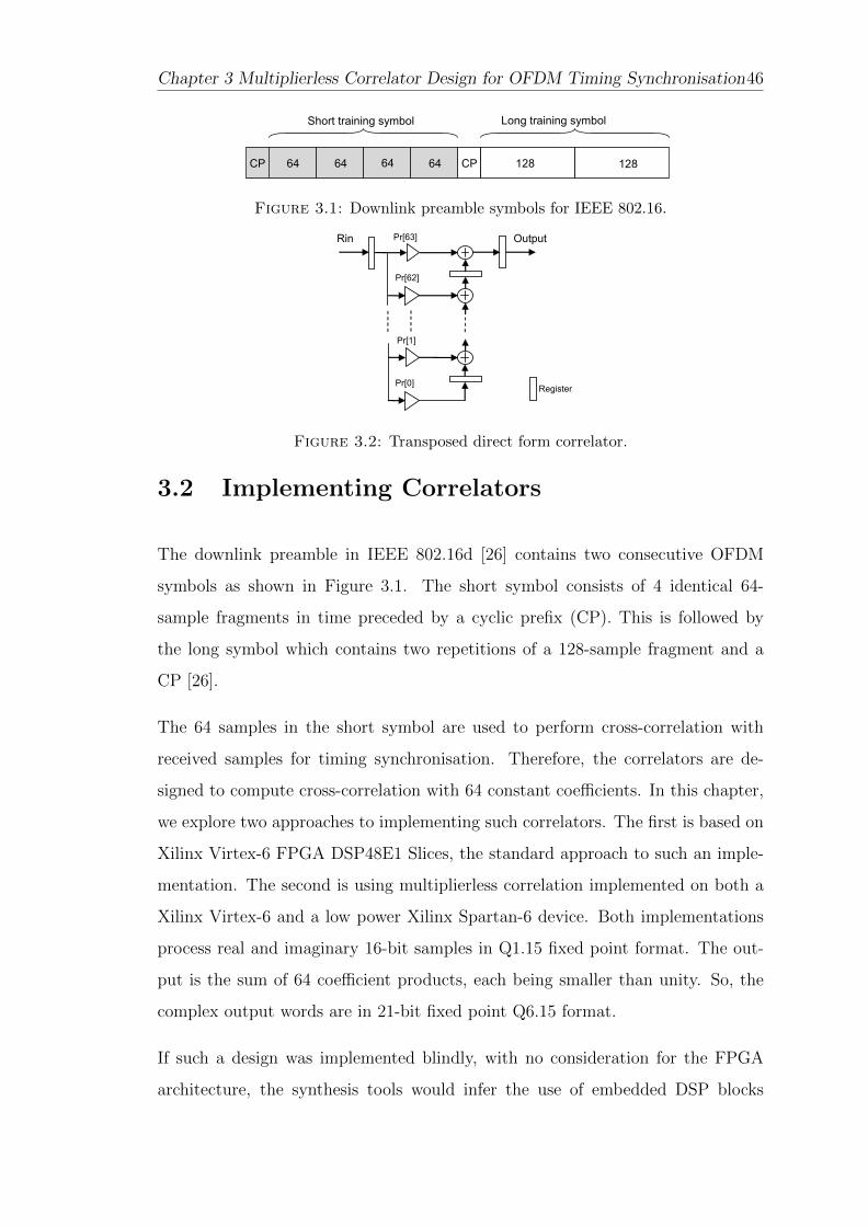
Chapter 3 Multiplierless Correlator Design for OFDM Timing Synchronisation46
CP CP64 64 64 64 128 128
Short training symbol Long training symbol
Figure 3.1: Downlink preamble symbols for IEEE 802.16.
Rin Output Pr[63]
Pr[62]
Pr[1]
Pr[0] Register
Figure 3.2: Transposed direct form correlator.
3.2 Implementing Correlators
The downlink preamble in IEEE 802.16d [26] contains two consecutive OFDM
symbols as shown in Figure 3.1. The short symbol consists of 4 identical 64-
sample fragments in time preceded by a cyclic prefix (CP). This is followed by
the long symbol which contains two repetitions of a 128-sample fragment and a
CP [26].
The 64 samples in the short symbol are used to perform cross-correlation with
received samples for timing synchronisation. Therefore, the correlators are de-
signed to compute cross-correlation with 64 constant coefficients. In this chapter,
we explore two approaches to implementing such correlators. The first is based on
Xilinx Virtex-6 FPGA DSP48E1 Slices, the standard approach to such an imple-
mentation. The second is using multiplierless correlation implemented on both a
Xilinx Virtex-6 and a low power Xilinx Spartan-6 device. Both implementations
process real and imaginary 16-bit samples in Q1.15 fixed point format. The out-
put is the sum of 64 coefficient products, each being smaller than unity. So, the
complex output words are in 21-bit fixed point Q6.15 format.
If such a design was implemented blindly, with no consideration for the FPGA
architecture, the synthesis tools would infer the use of embedded DSP blocks

Chapter 3 Multiplierless Correlator Design for OFDM Timing Synchronisation47
for multiplication, but would likely achieve poor timing performance due to an
inability to optimise the use of the DSP block. The DSP48E1 primitives on the
Virtex-6 FPGAs have additional circuitry within them that enables the design
of optimised datapaths, but this must be done manually, through writing code
in a particular style. Otherwise, the synthesis tools cannot always infer the most
efficient structure. In our design, we have taken into account the internal structure
of the DSP block, and made the design as lean as possible. The correlator designs
must be specified manually, and cannot be inferred by the tools from higher level
descriptions such as high level synthesis (HLS) or Simulink. We instead use Verilog
with wordlengths and schedules selected to mirror the structure of the DSP block.
3.2.1 Design of DSP48E1 Based Correlator
The DSP48E1 block inside the Virtex-6 shown in Figure 3.3 contains a multiplier
followed by a configurable arithmetic unit to provide many independent functions,
e.g., multiply, multiply-accumulate, multiply-add, three-input add, and more [2].
It also allows the datapath to be configured for various input combinations and
register stages; a three-stage pipeline offers maximum performance. Since the
DSP block is designed to mirror the structure of an FIR filter tap, it is ideally
suited to implement correlation, and would hence be the method of choice for
this application. Our first design uses non-pipelined DSP48E1 blocks in transpose
direct form, as shown in Figure 3.2, with 64 coefficients corresponding to the 64
samples in the preamble. The coefficients are pre-computed according to the IEEE
802.16d specification. The second design spreads the complex multiply-adds in a
five-stage pipeline, shown in Figure 3.4, consisting of DSP48E1 blocks configured
for three stage internal pipelining. Ri Re, Ri Im are the real and imaginary parts
of the received sample, respectively. Pr Re, Pr Im similarly represent known
preamble. The pipeline registers for the Pr Re, Pr Im are eliminated because
they have a constant value. Re, Im are the real and imaginary parts of the previous
multiply-add. Figure 3.5 presents the pipeline structure of the correlator. The

Chapter 3 Multiplierless Correlator Design for OFDM Timing Synchronisation48
Figure 3.3: Structure of DSP48E1 block inside the Virtex-6 [2].
Register
Intrinsic Register of DSP48E1
Pr_Im
Ri_Re
Pr_Re Ri_Im
Imaginary
Im
Pr_Im
Ri_Im
Ri_Re Pr_Re
Real
Re
Figure 3.4: Pipeline structure of the complex number multiply-add.
Rin 0
Pr [1]
Pr [2]
Pr [0]
Pr [63] output
Complex multiply-add
Complex multiply-add
Complex multiply-add
Complex multiply-add
Figure 3.5: Pipeline structure of correlator using DSP48E1 blocks.
additional pipeline registers are required to handle the received sample. Adding
pipeline registers should increase performance significantly.

Chapter 3 Multiplierless Correlator Design for OFDM Timing Synchronisation49
Register
Shift_Add
Pr[63]
Pr[62]
Pr[1]
Pr[0]
Rin Output
Figure 3.6: Structure of multiplierless correlators.
3.2.2 Design of Multiplierless Correlator
The principle of multiplierless correlators is to represent the coefficients and round
them in the form of summed powers of two. Hence, shifts and additions are per-
formed instead of multiplying by coefficients. It is expected that multiplierless cor-
relation is more efficient, but with embedded hard multipliers in modern FPGAs,
it is unclear whether they should still be considered favourable. Furthermore,
synchronisation accuracy must be considered. To explore this, four alternative
multiplierless correlators are implemented using four coefficient sets with an in-
creasing degree of rounding, to compare the cost and performance and evaluate
against multiplier-based correlators. The coefficient sets are found by quantising
the 64 normalised preamble samples with quantisations of 1, 0.5, 0.25, and 0.125.
The proposed structure for multiplierless correlators is shown in Figure 3.6. This
structure is based on the transposed direct form shown in Figure 3.2. Instead of
using multipliers to multiply input samples by coefficients, the Shift Add block
and multiplexers are used to perform the equivalent operation without an actual
multiplication. The Shift Add block, multiplexers and value of Pr[n] are different
depending upon the quantised coefficient set being used, and these perform shifts
and additions on received samples according to the degree of quantisation that is
applied. To optimise resources in the case of small numbers of bit quantisation,
one common Shift Add block is used for all 64 coefficients instead of 64 separate

Chapter 3 Multiplierless Correlator Design for OFDM Timing Synchronisation50
Shift Add blocks. This common Shift Add block calculates all possible values for
64 coefficients. The multiplexers are used to select the corresponding Shift Add
outputs to accumulate in order to generate the correlator output. These are based
on expressed coefficients Pr[n] that are pre-computed based on quantizing the 64
preamble samples. Since the Pr[n] values are constants, after synthesising the
design, the multiplexer is optimised as hard-wired logic, and the preamble cannot
be changed. To support different OFDM preambles, the Pr[n] could be stored in
a register, and a real multiplexer used instead of hard-wired logic. This results in
increased resource utilisation but provides a more flexible solution.
3.2.3 Implementation Results
The designs presented were synthesised and fully implemented using Xilinx ISE
13.2, targeting Xilinx Virtex-6 (V6) and Spartan-6 (S6) devices. The results of
implementation are reported in terms of the number of occupied slices, DSP48E1s
blocks and maximum frequency as summarised in Table 5.1.
Table 3.1: Resource utilisation summary.
Design Slices DSP48E1s Freq. (MHz)
V6 S6 V6 V6 S6
DSPc 742 (6%) - 256 (88%) 119 -
DSP pp 1,110 (9%) - 256 (88%) 398 -
ML1 661 (5%) 762 (6%) 0 (0%) 309 174
ML2 983 (8%) 1,071 (9%) 0 (0%) 268 158
ML3 1,191 (10%) 1,257 (10%) 0 (0%) 234 136
ML4 1,496 (12%) 1,517 (13%) 0 (0%) 208 124
DSPc, DSP pp are correlator designs using DSP Slices, in non-pipelined and
pipelined structures, respectively. ML1, ML2, ML3, ML4 are multiplierless corre-
lators with coefficient quantisations of 1, 0.5, 0.25, 0.125, respectively. The DSP48
is typically used for multiplication in fixed point format, Q1.15 (1 integer and 15
fractional bits). Because the DSP48 is a hard core, it is impossible to optimise

Chapter 3 Multiplierless Correlator Design for OFDM Timing Synchronisation51
the internal components of the DSP48 by reducing the number of bits used in
the computation. The static power of the DSP block based correlator does not
drop significantly in this case. Thus the use of DSP48 for calculation of words
with fewer bits is wasteful in terms of resources and results in reduced precision.
Hence, we do not consider the DSP48 version when comparing implementations
with a small number of bits.
Table 5.1 reveals that the DSP pp uses more logic slices due to its pipelined struc-
ture. The slices in DSP48E1 based designs are used for registers and route-thrus
while the slices in the multiplierless designs are mostly used as logic. The number
of slices used in the multiplierless designs increases as the coefficient quantisation
becomes finer. The DSP48E1-based designs use 256 DSP Slices, 4 for each complex
multiply plus 6-9% of logic resources. The multiplierless designs use only logic to
compute the cross correlation with 64 complex coefficients. The total logic area
is a small fraction of the whole device: around 5-12% of total resources in the
Virtex-6, and around 6-13% of total resources in the equivalent Spartan-6. While
Spartan-6 devices do include DSP Slices, their number is insufficient to implement
the full 64 sample complex cross correlation. This shows an ideal scenario where
multiplierless correlation makes sense, and hence serves as a motivation for this
study.
The maximum frequencies, reported after place and route, decrease for multipli-
erless designs according to the degree of coefficient quantisation. Meanwhile the
non-pipelined DSP48E1 design is slower than the multiplierless designs. However,
the pipelined DSP48E1 design can achieve significantly higher frequency. The
multiplierless correlator and the DSP-based correlator can both operate at fre-
quencies multiple times higher than required for baseband modulation. Therefore,
both designs could use time multiplexing of the computational resources to trade-
off resource usage and operating frequency. However, it should be noted that
increased operating frequency leads to significantly increased power consumption
since the power consumption is proportional to the square of switching frequency.
To provide a fair comparison, both the multiplierless correlator and the DSP-based
correlator are investigated using the same transposed direct form.

Chapter 3 Multiplierless Correlator Design for OFDM Timing Synchronisation52
A post-place-and-route simulation in ModelSim was used to estimate the power
consumption of the system using the Xilinx XPower tool. Table 3.2 shows the
power dissipation of the designs running at 50 MHz. The DSP48E1-based correla-
tors consume more power than the multiplierless correlators, but this is due pri-
marily to increased dynamic power when using the DSP48E1s on the Virtex-6. The
dynamic power of the non-pipelined DSP48E1-based correlator DSPc is greatest
at 846 mW, but pipelining reduces this by a factor of more than 2.5 times, due to
reduced switching activity between the multiplier and adder. The dynamic power
of the multiplierless designs increases from 133 mW to 203 mW on the Virtex-6
and from 149 mW to 294 mW on Spartan-6 as finer coefficient quantisation is used.
It is important to note that the quiescent power of the Spartan-6 is much lower
by design. Hence, we can see that using this multiplierless technique allows us to
implement synchronisation on a Spartan-6 device, where a multiplier-based design
is not possible due to resource limitations, while also saving significant power. In
the next section, we will evaluate the impact on accuracy.
Table 3.2: Correlator power consumption at 50 MHz.
Correlators Quiescent(mW) Dynamic(mW) Total(mW)
V-6 S-6 V-6 S-6 V-6 S-6
DSPc 1312 - 846 - 2158 -
DSP pp 1300 - 328 - 1628 -
ML1 1296 67 133 149 1429 216
ML2 1296 68 160 197 1456 265
ML3 1297 70 182 239 1479 309
ML4 1297 71 203 294 1500 365
We also investigated how total power consumption varies with frequency, as shown
in Figure 3.7. As frequency increases, the finer quantisations and DSP48E1-based
designs begin to consume proportionally more power. Overall, multiplierless de-
signs on the Spartan-6 consume 75% to 85% less power than the same designs on
the Virtex-6, and a 0.25 quantisation design on the Spartan-6 consumes 81% to
85% less power then the DSP48E1-based design on a Virtex-6.

Chapter 3 Multiplierless Correlator Design for OFDM Timing Synchronisation53
Figure 3.7: Correlator power consumption at different frequencies.
The DSPc implementation represents how an architecture-independent design
would be mapped. Our architecture-aware designs show significantly improved
performance, reduced area, and reduced power consumption.
3.3 Simulation and Discussion
In order to validate our designs at the application level, we simulate them using
ModelSim with an IEEE 802.16 OFDM frame created using MATLAB, including
the preamble symbols, data symbols and effects of an AWGN channel. Cross-
correlation results using the correlator designs are compared to corresponding
results in MATLAB to verify the correctness of implementation. To evaluate the
accuracy of timing synchronisation achievable by these designs, the correlation
outputs are plotted in Figure 3.8 for random data frames at 10 dB SNR. The
output of each correlator is slightly different because of rounding, but the timing
synchronisation depends upon the location of the peaks being at the position of
the preamble. All correlator designs achieve this most of the time, as shown at
indices 34 and 98 for the CP samples and the first preamble samples respectively,
for a single frame.

Chapter 3 Multiplierless Correlator Design for OFDM Timing Synchronisation54
Figure 3.8: Correlator output with SNR = 10 dB.
In order to evaluate the synchronisation accuracy of these approaches, we simulate
10,000 correlation operations in an AWGN channel with a detection strategy as
follows. First, find the first peak, P1, over 64 samples. Next, find the second peak,
P2, in the 64 samples following the first peak and compute the average value, avg,
of the samples between two peaks. If (P1 − avg) ≤ 0.75 ∗ (P2 − avg), the start
of frame is detected and the correctness of the position can be checked. It should
be noted that in all cases, the peaks were known to be located within the two
search regions and that the detection strategies described above are compatible
with those in other published work such as [4] and [92]. Figure 3.9 plots the
results in terms of failure rate against AWGN SNR and shows that the designs
are able to accurately detect the start of frame even in low SNR conditions. The
failure rate of ML1 is the highest, as expected, due to the coarse quantisation.
For SNRs above 4 dB, the failure rates of ML2, ML3, ML4, and DSPc differ less
than 0.05% from each other. This suggests that sacrificing arithmetic accuracy
by using multiplierless cross-correlation is feasible and has negligible impact on
synchronisation accuracy. Combined with the results in the previous section, we
can be confident that low-power FPGAs, such as the Spartan-6, with insufficient
resources for multiplier-based correlation, are still feasible for implementing robust
OFDM receivers.
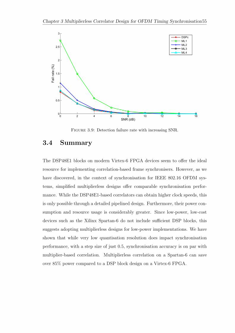
Chapter 3 Multiplierless Correlator Design for OFDM Timing Synchronisation55
Figure 3.9: Detection failure rate with increasing SNR.
3.4 Summary
The DSP48E1 blocks on modern Virtex-6 FPGA devices seem to offer the ideal
resource for implementing correlation-based frame synchronisers. However, as we
have discovered, in the context of synchronisation for IEEE 802.16 OFDM sys-
tems, simplified multiplierless designs offer comparable synchronisation perfor-
mance. While the DSP48E1-based correlators can obtain higher clock speeds, this
is only possible through a detailed pipelined design. Furthermore, their power con-
sumption and resource usage is considerably greater. Since low-power, low-cost
devices such as the Xilinx Spartan-6 do not include sufficient DSP blocks, this
suggests adopting multiplierless designs for low-power implementations. We have
shown that while very low quantisation resolution does impact synchronisation
performance, with a step size of just 0.5, synchronisation accuracy is on par with
multiplier-based correlation. Multiplierless correlation on a Spartan-6 can save
over 85% power compared to a DSP block design on a Virtex-6 FPGA.

Chapter 4
Method for OFDM Timing
Synchronisation
4.1 Introduction
OFDM performance is sensitive to receiver synchronisation [93]. Frequency offset
causes inter-subcarrier interference, and errors in timing synchronisation can lead
to inter-symbol interference. Therefore, accurate synchronisation is critical to the
performance of OFDM systems. This section summarises conventional synchroni-
sation methods used with OFDM, discussing their merits and drawbacks, before
the following sections present a new and efficient method that is robust to large
frequency offset, obtains accurate and robust synchronisation and requires rela-
tively low computational complexity. In particular, it is designed to be suitable
for hardware implementation on reconfigurable systems.
The method presented in this chapter has also been discussed in:
• T. H. Pham, I. V. McLoughlin, and S. A. Fahmy, “Robust and Efficient
OFDM Synchronisation for FPGA-Based Radios,” in Circuits, Systems, and
Signal Processing, vol. 33, no. 8, pp. 2475 - 2493, Aug. 2014, Springer [94].
56

Chapter 4 Method for OFDM Timing Synchronisation 57
4.2 Related Work
Autocorrelation-based methods are commonly chosen for implementing synchro-
nisation because of their low computational complexity. In [3], timing metrics are
defined as follows, beginning with the normalised power measure M[d] :
M [d] =|P [d]|2(R[d])2
, (4.1)
where d denotes a time index corresponding to the first sample in a search space
comprising 2L samples of received signal r. The power measure R, which represents
the energy of the second half of the receiver search window, is defined as:
R[d] =L−1∑m=0
|r[d+m+ L]|2, (4.2)
and the normalisation parameter P computes the correlation between two periodic
halves in the search window as:
P [d] =L−1∑m=0
(r∗[d+m]r[d+m+ L]), (4.3)
The metric M[d] is illustrated for a typical channel in Figure 4.1, where it can
be seen to form a distinct plateau in the region when the preamble is presented
within a received window. Clearly, M[d] accurately detects the preamble, however
the nature of the plateau having a flat top presents an uncertainty in terms of
exact positioning, and hence reduced accuracy in determining the exact start of
the frame, compared to a metric which peaks.

Chapter 4 Method for OFDM Timing Synchronisation 58
−100 −50 0 50 100 150 200 250 3000
0.1
0.2
0.3
0.4
0.5
0.6
0.7
0.8
0.9
1
Sample Index d
Val
ue o
f Tim
ing
Met
ric
Figure 4.1: The timing metric in [3] applied to the IEEE 802.16-2009 preamblein an AWGN channel (SNR = 10dB)
In order to improve the accuracy of synchronisation, a scheme is often used as
in [95, 96, 14, 42, 15] based on combining the above metric for detecting the
frame, estimated coarse STO and fractional CFO, and additional cross-correlation
operations for computing fine STO and integer CFO as we will explore below.
4.2.1 Coarse STO and Fractional CFO Estimation
First, the plateau of the M[d] metric is used to detect a frame start and estimate
coarse STO by comparing the magnitude of M[d] to a given threshold. After
this, the CFO is estimated using the P metric in (4.3). We now assume that we
are receiving a signal s[d] which has a normalised carrier frequency offset ξ with
respect to r[d] :
s[d] = ej2πξdN ∗ r[d]. (4.4)

Chapter 4 Method for OFDM Timing Synchronisation 59
where N is the numbers of subcarriers of the OFDM symbol. At the plateau of
M[d], the received samples in the window will be periodic:
r[d] = r[d+ L]. (4.5)
Substituting (4.4) and (4.5) in (4.3) we find that
P [d] =L−1∑m=0
(s∗[d+m]s[d+m+ L])
= ej2πξLN
L−1∑m=0
|r[d+m]|2 (4.6)
The CFO can be determined as follows;
ξ =∠P [d] + 2πz
2π LN
(4.7)
where ∠P [d] is the angle of P[d] within the range -π to π. The CFO consists of 2
parts: the fractional part, λ = ∠P [d]
2π LN
, can be estimated replied on ∠P [d] and the
integer part (IFO) is represented by an integer z, ε = zNL
. The fractional CFO
estimation has a range limitation as follows:
− N
2L< λ <
N
2L(4.8)
Clearly, the range over which fractional CFO can be estimated may be increased
by decreasing the length of period L. However, because of the influence of channel
noise, a smaller L would also degrade the accuracy of estimation of the fractional
CFO λ. In the case of the IEEE 802.16-2009 preamble [26], the number of sub-
carriers N and length of period L are commonly chosen to be 512 and 64 samples
respectively [13]. Hence the fractional CFO estimation range is limited to within

Chapter 4 Method for OFDM Timing Synchronisation 60
-2 to +2 subcarrier spacings. Meanwhile, the value of IFO parts ε is estimated as
an integer multiple of 4.
The method outlined above is fast and robust for estimating coarse STO and frac-
tional CFO. However it has some drawbacks. First, the coarse STO is estimated
by comparing the metric to a threshold. It is not certain that the samples for
estimating the fractional CFO are within the plateau of M[d] in which the re-
ceived samples in the window will be periodic. This degrades the performance of
fractional CFO estimation. Second, the CFO estimation can only be performed
correctly in the limited range of the fractional CFO shown in (4.8). If the actual
CFO lies outside this range, it is necessary to estimate the integer CFO separately.
4.2.2 Fractional CFO Compensation
Fine STO estimation, accomplished using cross-correlation, is sensitive to CFO.
Thus the estimated fractional CFO must first be used for frequency offset com-
pensation. This is done by phase de-rotating the received samples in the time
domain:
r[d] = e−j2πξd′N ∗ s[d]; d′ = d+ toff . (4.9)
r[d] and s[d] are the compensated samples and frequency offset samples, respec-
tively. d’ is the coarse estimated timing index that differs from the correct timing
index toff samples. Substituting (4.4) in (4.9), we get:
r[d] = e−j2πξ(d+toff )
N ∗ ej2πξ dN ∗ r[d]
= e−j2πξtoffN ∗ r[d]. (4.10)

Chapter 4 Method for OFDM Timing Synchronisation 61
When compensating the fractional CFO, the fine STO has still not been estimated.
This results in a common phase error within the coarse CFO compensated samples
as shown in (4.10).
4.2.3 Fine STO Estimation
The purpose of timing synchronisation is to find the correct starting point for
receiver demodulation. This starting point will generally mark the beginning of
a discrete Fourier transform (DFT) window. Coarse time synchronisation is com-
monly based on auto-correlation as mentioned above, leading to relatively simple
hardware implementation. However, with purely coarse STO, it is almost impossi-
ble to achieve sufficient accuracy to correctly detect the starting point. Thus, fine
STO estimation is necessary to refine the accuracy of timing synchronisation. To
obtain more accurate fine STO estimation, cross-correlation is usually performed
between the received samples and known transmitted preamble. The peak cross-
correlation occurs when the received samples match the known preamble. Fine
STO can thus be found by locating this peak within a search window. In order to
reduce the overhead of cross-correlation, a sign bit multiplier can be used instead
of a real multiplier to calculate cross-correlation. However, this is much more sen-
sitive to CFO in practice [95]. Some researchers employ enhanced methods based
on cross-correlation for the time synchronisation. For example, Kishore and Reddy
[4] presented an algorithm using cross-correlation between the known transmitted
and received preamble symbols. The timing metrics for synchronisation using this
method perform the normalised M[d] calculation, and use the same denominator
R as in (4.1) and (4.2), however they refine the numerator P as follows;
P [d] =L−1∑m=0
(r[d+m]a[m])∗(r[d+m+ L]a[m]), (4.11)

Chapter 4 Method for OFDM Timing Synchronisation 62
where d again denotes the time index corresponding to the first sample in a win-
dow of 2L samples of received signal r and superscript “∗”again denotes complex
conjugation. In (4.11) the samples a are now the known, transmitted, time domain
preamble samples.
The cross correlation now produces distinct peaks at the times when received sam-
ples match the known transmitted samples of the preamble. Figure 4.2 illustrates
this by plotting M versus the sample index d for an example channel in AWGN
with SNR = 10 dB. A frame is detected when M crosses a threshold and the start
of frame is found by searching the peaks of M. This can accurately determine the
start of frame even at low SNRs. Moreover, this method is robust to large CFO
for time synchronisation. Simulations [4] show that time synchronisation can be
performed effectively with CFO = 10.5 subcarrier spacings. However, the cross-
correlation operation requires complex computation. Although the complexity of
cross-correlation can be reduced using multiplierless correlation [92], the multipli-
erless correlator degrades the precision of metric P, used for estimating frequency
offset. In general, this method is appropriate for time synchronisation but requires
significant hardware resources for implementing the cross-correlation.
4.3 Proposed Fractional CFO Estimation and Syn-
chronisation
Considering the limitations of previous work, we propose new timing metrics to
take advantage of preamble characteristics such as period and energy distribution.
Again, the proposed method is illustrated for the specific case of the IEEE 802.16-
2009 preamble, as shown in Figure4.4.
Firstly, we define the autocorrelation between the two halves of the receiver window
for normalisation purposes;
P ′[d] =C−1∑m=0
(r∗[d+m]r[d+m+ L]) (4.12)

Chapter 4 Method for OFDM Timing Synchronisation 63
−100 −50 0 50 100 150 200 250 3000
0.5
1
1.5
2
2.5
3
3.5
4
4.5
Sample Index d
Val
ue o
f Tim
ing
Met
ric
Figure 4.2: The timing metric in [4] applied to the IEEE 802.16 preamble inan AWGN channel (SNR = 10dB)
where d denotes a time index of received signal r that now corresponds to the
first sample in a window of L+C samples of received signal, L being the length
of preamble period (64 for the IEEE802.16 preamble) and C being the length of
received samples for estimation, respectively.
Next, a power measure, R’ is proposed which takes account of both received and
transmitted symbol power;
R′[d] =C−1∑m=0
|r[d+m+ L]|2|a[m]|2 (4.13)
In common with the metric developed by Schmidl and Cox [3], our proposed P’[d]
detects the periodic characteristic of the preamble and can thus be used for es-
timating fractional CFO. P’ forms a plateau as evident in Figure4.3 when the
preamble is present within the receiver window. R’ is then used to find the start-
ing point of the preamble based on its energy distribution. R’ causes peaks shown
in Figure4.3 at the point where the energy distribution of the received samples
matches that of the transmitted preamble. Since the R’ metric that is used to

Chapter 4 Method for OFDM Timing Synchronisation 64
−100 −50 0 50 100 150 200 250 300
0
0.2
0.4
0.6
0.8
Sample index d
Val
ue
ofT
imin
gM
etri
c
P’ Metric R’ Metric
Figure 4.3: Proposed timing metrics applied to the IEEE 802.16 preamble inAWGN (SNR = 10 dB, CFO = 10.5).
estimate time synchronisation is computed on the square of the amplitude of re-
ceived samples, the time synchronisation is insensitive to the CFO that effects
the phase of the received samples. Moreover, computing on amplitude squared, a
real number, requires less resources than using complex numbers as in alternative
approaches such as [4]. In addition, the time synchronisation is performed based
on the peak value of R’ rather than its absolute value. Therefore, R’ is a good
candidate for implementation using a multiplierless correlator to reduce computa-
tional complexity. Figure4.4 illustrates the flow of the proposed synchronisation
method according to the received samples of the preamble, compared to that of
the conventional scheme. As can be seen in the conventional scheme, the coarse
STO and fractional CFO estimation are performed in the two first periods of the
short training symbol from (i) to (iii), and then the estimated fractional CFO is
used for compensation. The fine STO is estimated in the last period of the short
training symbol from (iv) to (vi), and integer CFO should be computed in the long
training symbol from (vii) to (viii). By contrast, the proposed method performs
STO synchronisation and fractional CFO estimation in the three first periods of
the short training symbol from (i) to (iv), and the start of frame will be detected
at (ii). Then, the fractional CFO compensation is computed, and integer CFO
estimation is performed in the long training symbol from (vii) to (viii).
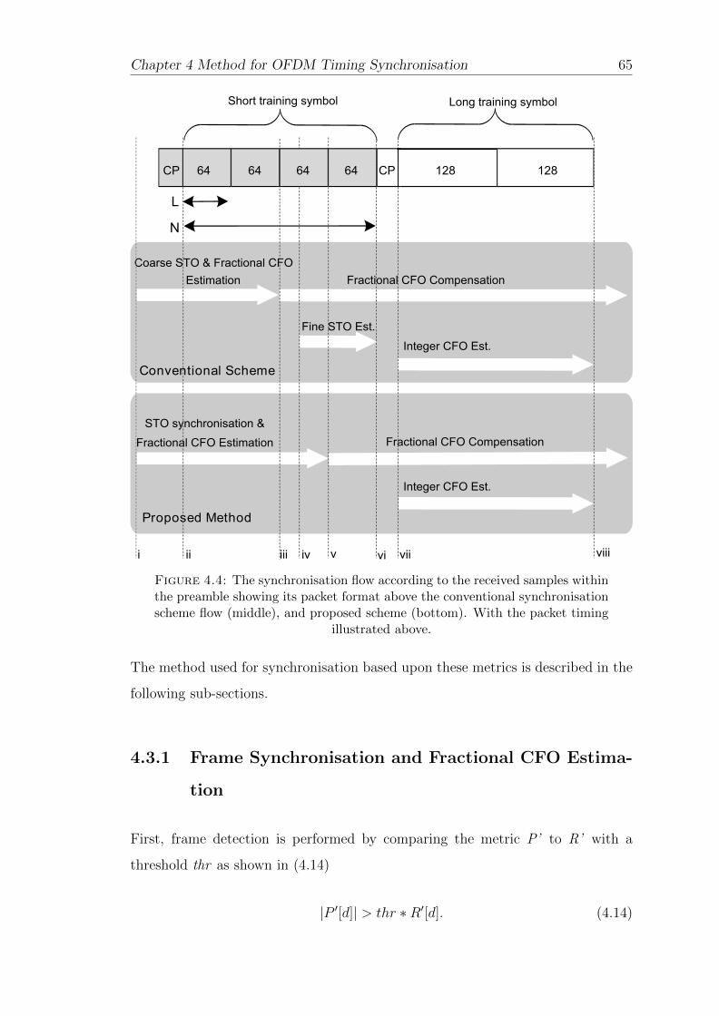
Chapter 4 Method for OFDM Timing Synchronisation 65
Integer CFO Est.
Fractional CFO Compensation STO synchronisation &
Fractional CFO Estimation
Fine STO Est.
Integer CFO Est.
Fractional CFO Compensation
Coarse STO & Fractional CFO
Estimation
L
N
Short training symbol Long training symbol
Conventional Scheme
Proposed Method
i ii iii iv v vi vii
CP CP64 64 64 64 128 128
viii
Figure 4.4: The synchronisation flow according to the received samples withinthe preamble showing its packet format above the conventional synchronisationscheme flow (middle), and proposed scheme (bottom). With the packet timing
illustrated above.
The method used for synchronisation based upon these metrics is described in the
following sub-sections.
4.3.1 Frame Synchronisation and Fractional CFO Estima-
tion
First, frame detection is performed by comparing the metric P’ to R’ with a
threshold thr as shown in (4.14)
|P ′[d]| > thr ∗R′[d]. (4.14)

Chapter 4 Method for OFDM Timing Synchronisation 66
0.2 0.3 0.4 0.5 0.6 0.7 0.8 0.9 10
100
200
300
400
500
600
700
800
900
1000
Threshold Value
Rat
e Number of correct detection
Number of false detection
Number of miss detection
Figure 4.5: Performance of the frame synchronisation method versus the se-lection threshold for an AWGN channel (with SNR =10dB).
Figure4.5 shows the performance of the frame synchronisation in the given channel
for different threshold values. With each threshold value, 1000 frame detections
are simulated. The number of correct detections indicates how often the time
synchronisation has been found correctly at the start of the frame, while the
number of false detections indicate that the time synchronisation gets the wrong
start of the frame. Otherwise, the frame is not detected (i.e. |P ′[d]| can be not
greater than thr∗R′[d]), and a miss detection is declared. From the results plotted,
the optimum value can be seen to be around 0.55. If the threshold is too small,
noise may cause a failure of detection. On the other hand, when the threshold
is large, the frame detection may be missed if the noise reduces the amplitude
of the timing metric, which consequentially does not cross the threshold. The
threshold values depend on the operating channel and are determined empirically
by simulation (in common with other systems such as in [36]). Assuming the set of
possible channels is known, the thresholds for these channels can be pre-determined
by simulation. The performance of synchronisation is evaluated with increased
thresholds for a given channel model. The threshold value corresponding to the

Chapter 4 Method for OFDM Timing Synchronisation 67
best performance is selected for the channel model. The determined threshold
values are stored in a look-up table. Based upon current channel model and
conditions, a threshold is selected from the look-up table.
After a frame is detected, the starting point of the short preamble is found by
searching for the peaks in R’[d]. As can be seen in Figure 4.3, two peaks in R’[d]
will bracket the transition to the plateau in P’[d] shown at sample indices of -31
and 33, respectively. The second peak is used as the starting point for the DFT
window. This is accomplished for the maximum values of R′[d] + R′[d − L] over
the next L samples after frame detection. Second, the fractional CFO estimation
is presented in (4.15) based on the P’[d] metric similarly to other work such as
[3, 95, 96, 14, 42, 15];
λ =∠P ′[d]
2π LN
(4.15)
where λ is the estimated fractional CFO, ∠P ′[d] denotes the angle of P’[d] and
N is the number of subcarriers. In this proposed method, the fractional CFO is
estimated at the starting point of the preamble to guarantee that the correct angle
of P’[d] is taken for estimation. Using the conventional techniques, the inherent
uncertainty in the coarse STO does not allow this to be achieved in practice. Thus,
the estimated fractional CFO in the proposed method will, on average, tend to be
more accurate. In addition, this method separates the length of preamble period
L and the length of received samples for estimation C, and because of that L can
be small to extend the range of fractional CFO, and C can be longer to increase
the robustness to channel noise. For the IEEE 802.16 preamble, C is set equal to
2L to improve the overall precision of synchronisation.
4.3.2 Fractional CFO Compensation
Compensating the fractional CFO is performed in the traditional way by phase
de-rotating the received samples in the time domain;

Chapter 4 Method for OFDM Timing Synchronisation 68
r[d] = e−j2π∆fcdTs ∗ s[d].
= e−j2πξdN ∗ ej2πξ dN ∗ r[d]
= r[d]. (4.16)
However, in this proposed method, the frame synchronisation is achieved before
performing fractional CFO compensation, therefore, toff is removed, and thus, the
common phase errors caused by fractional CFO compensation are missing. The
compensated received samples are then demodulated using the DFT to obtain the
received symbols in the frequency domain.
4.3.3 Simulation Results and Discussion
In this section, we will evaluate the performance of the proposed synchronisation
method, applied to the IEEE 802.16-2009 downlink preamble, in MATLAB under
both AWGN channels as well as the more realistic SUI channels that are widely
used in the research literature [4, 13].
The Stanford University Interim (SUI) channel model [97] is used to simulate a
frequency selective channel and takes into account many wireless channel effects
including delay spread, Doppler spread, phase noise, and channel interference.
In addition, the value of metrics computed in MATLAB are later verified with
corresponding values from the FPGA simulation, to ensure practical functional
equivalence.
In total, 100,000 OFDM frames, preceded by noise with randomly seeded AWGN
and followed by preamble and data symbols, are used to evaluate synchronisation
performance for each method. The proposed method is compared to the state of
the art method, in terms of accuracy of both time synchronisation and fractional
CFO estimation. The performance of STO estimation is measured in terms of
failure rate (%), and the accuracy of CFO estimation is evaluated in terms of mean

Chapter 4 Method for OFDM Timing Synchronisation 69
square error (MSE). We separately evaluate the robustness of time synchronisation
against large CFO for each method. Three versions of the proposed approach are
constructed by varying the length, C, of received samples for estimation based on
(4.12). These are investigated to determine the tradeoff between accuracy and
computational cost, with C defined as follows in each case:
• Prop 1 : C = L
• Prop 2 : C = 2L
• Prop 3 : C = 3L
These are compared to the state of the art method (denoted as SoA) [85, 15],
and the method of Kishore and Reddy [4] (denoted as K&R) for a number of
evaluation scenarios. First, the performance of each method is found for AWGN
channels beginning with CFO = 0.5, then AWGN channels with CFO varying from
-10 to +10 times carrier spacing, then SUI1, and finally SUI2 channels.
4.3.3.1 Performance in AWGN
0 2 4 6 8 10 12 14 1610−3
10−2
10−1
100
101
102
SNR(dB)
Fai
lra
teof
fram
esy
nch
ronis
atio
n(%
)
Prop3 Prop2 Prop1SoA K&R
Figure 4.6: Performance of time synchronisation in AWGN channels with afrequency offset of 0.5 subcarrier spacings.

Chapter 4 Method for OFDM Timing Synchronisation 70
0 2 4 6 8 10 12 14 16
10−4
10−3
10−2
SNR(dB)
MSE
ofF
ract
ional
CF
O
Prop3 Prop2 Prop1SoA K&R
Figure 4.7: Performance of fractional frequency offset estimation in AWGNchannels.
Figure 4.6 and Figure 4.7 plot the performance results of STO and CFO estimation
in AWGN with a frequency offset of 0.5 subcarrier spacings, respectively. SoA
and the proposed methods have much better performance than K&R in these
tests, achieving perfect synchronisation when SNR exceeds 5 dB. Prop1 ’s STO
estimation has slightly better accuracy with SNR below 3 dB but is worse at
higher SNR than SoA. Increasing the length of received samples for estimation,
i.e., setting C = 2L, allows Prop2 to obtain a remarkable improvement in STO
estimation, clearly better than the estimation achievable by SoA. Prop3, with
C = 3L, demonstrates decreasing gains: it is not able to enhance accuracy as
much as Prop2, despite a considerable hardware cost incurred when increasing
C. In addition, the CFO of Prop3 and Prop2 achieve significant improvement
compared to the other methods in Figure 4.7, while the accuracy of Prop1 and
SoA are identical (the curve for Prop1 is hidden behind the curve for SoA as a
result).
The gap between Prop1 and Prop2 is much larger than that between Prop2 and
Prop3, again demonstrating decreasing gains as C is extended. Thus, increasing C
from L to 2L is a more effective improvement than extending C from 2L to 3L. The
accuracy of CFO estimation in Prop2 is improved by about 5 dB in comparison
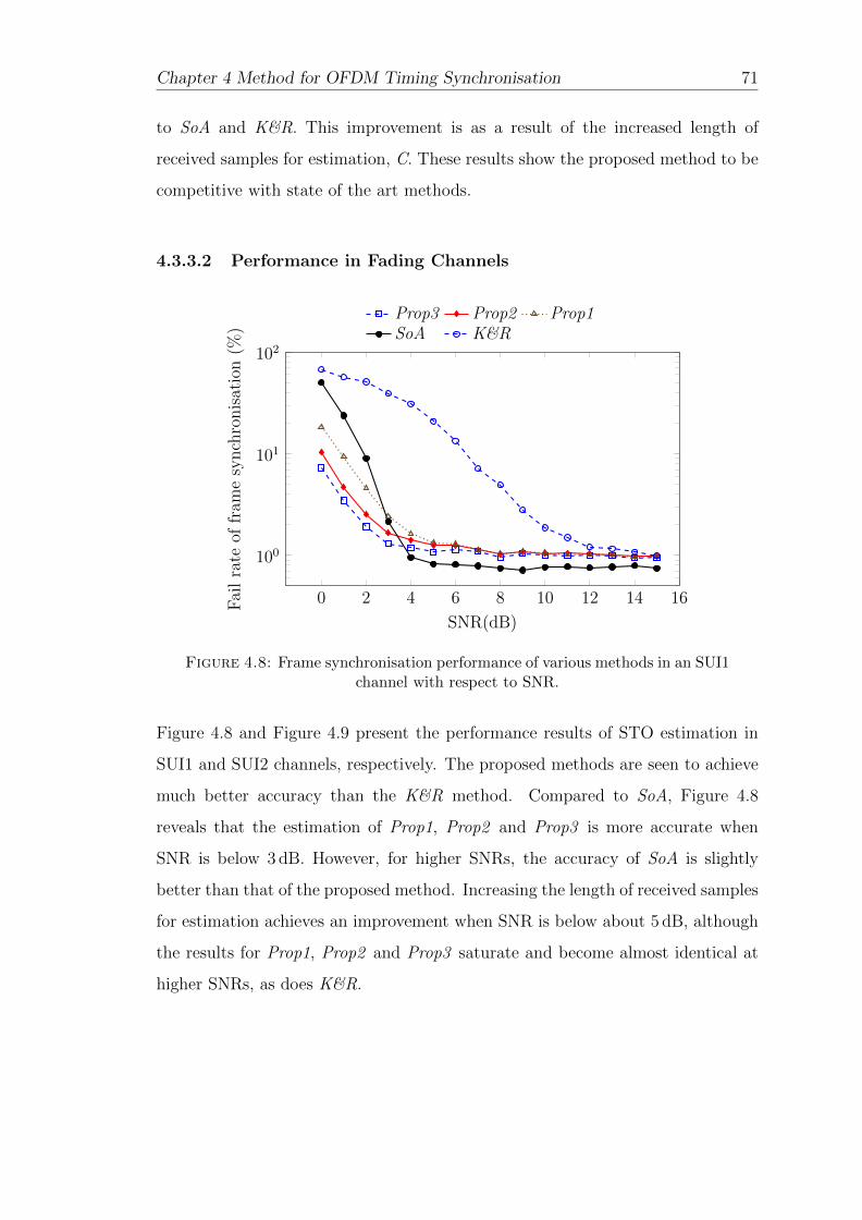
Chapter 4 Method for OFDM Timing Synchronisation 71
to SoA and K&R. This improvement is as a result of the increased length of
received samples for estimation, C. These results show the proposed method to be
competitive with state of the art methods.
4.3.3.2 Performance in Fading Channels
0 2 4 6 8 10 12 14 16
100
101
102
SNR(dB)
Fai
lra
teof
fram
esy
nch
ronis
atio
n(%
)
Prop3 Prop2 Prop1SoA K&R
Figure 4.8: Frame synchronisation performance of various methods in an SUI1channel with respect to SNR.
Figure 4.8 and Figure 4.9 present the performance results of STO estimation in
SUI1 and SUI2 channels, respectively. The proposed methods are seen to achieve
much better accuracy than the K&R method. Compared to SoA, Figure 4.8
reveals that the estimation of Prop1, Prop2 and Prop3 is more accurate when
SNR is below 3 dB. However, for higher SNRs, the accuracy of SoA is slightly
better than that of the proposed method. Increasing the length of received samples
for estimation achieves an improvement when SNR is below about 5 dB, although
the results for Prop1, Prop2 and Prop3 saturate and become almost identical at
higher SNRs, as does K&R.

Chapter 4 Method for OFDM Timing Synchronisation 72
0 2 4 6 8 10 12 14 16
100
101
102
SNR(dB)
Fai
lra
teof
fram
esy
nch
ronis
atio
n(%
)
Prop3 Prop2 Prop1SoA K&R
Figure 4.9: Frame synchronisation performance of various methods in an SUI2channel with respect to SNR.
0 2 4 6 8 10 12 14 1610−3
10−2
10−1
100
101
102
SNR(dB)
Fai
lra
teof
fram
esy
nch
ronis
atio
n(%
)
Prop3 Prop2 Prop1SoA K&R
Figure 4.10: Performance of frame synchronisation in an AWGN channel withuniform random frequency offset varying from -10 to 10 times carrier spacing,
with respect to SNR.
4.3.3.3 Performance with Large Frequency Offset
The proposed method is designed to work even with large frequency offsets. Fig-
ure 4.10 explores performance over 100,000 tests where the frequency offset is

Chapter 4 Method for OFDM Timing Synchronisation 73
chosen randomly (with uniform distribution) from -10 to +10 times the subcar-
rier spacing for each test, in an AWGN channel. This experiment is specifically
designed to investigate the robustness of STO estimation in large CFO conditions
and shows that the proposed methods still maintain good performance. K&R ex-
hibits some accuracy degradation, however, all methods are seen to outperform
SoA. The proposed methods are therefore seen to offer robustness of STO estima-
tion against large CFO. This robustness against large CFO is because the proposed
metric is computed on magnitude values that are insensitive to phase errors. CFO
estimation is not evaluated here because large CFO estimation requires an integer
CFO estimator that is investigated in the subsequent section.
In summary, simulation results show that Prop3 and Prop2 have better STO and
CFO estimation accuracy compared to other methods. Prop3 enjoys just a small
improvement in terms of STO estimation compared to Prop2 but this improve-
ment incurs a significant hardware cost because the length of received samples
for estimation must increase from 2L to 3L. Given the results described in this
sub-section, Prop2 is selected as an implementation candidate in the subsequent
sub-section, where the trade-off between accuracy and hardware cost is explored
in more detail.
4.3.4 Hardware Implementation
This sub-section discusses the implementation of, and presents the hardware op-
timisation of, the proposed method in terms of word size. The target FPGA is
a low-power Xilinx Spartan-6 XC6SLX45 device, with ISE 13.2 used to evaluate
both hardware resource and power consumption. The results illustrate the trade-
off between hardware consumption and the accuracy of the proposed method. The
above sub-section already revealed that the performance of K&R is generally worse
than the other methods, moreover it requires many complex multiply operations
to compute the cross-correlation for the P Metric. For this reason, K&R is not
implemented, only the proposed method and SoA are compared here, in terms of
hardware resources, power consumption, and accuracy. As mentioned above we

Chapter 4 Method for OFDM Timing Synchronisation 74
set C = 2L since Prop2 consistently showed performance close to Prop3, and sig-
nificantly better than Prop1. It therefore offers a good balance between increased
hardware cost and performance.
4.3.4.1 Implementation of Conventional Synchroniser
First, let us consider a conventional synchroniser. We have implemented this as
shown in Figure 4.11, following the efficient implementation methods presented
in [96, 41, 14, 85]. The P and R timing metrics in (4.3) and (4.2), respectively
are computed using delay and summation, whilst a very efficient signed bit mul-
tiplier [95] is used to significantly reduce the computational overhead of the cross
correlation for fine timing synchronisation.
Figure 4.11: Architecture of the conventional synchronisation FPGA imple-mentation.
We assume a 16-bit two’s complement fixed point representation with 15 frac-
tional bits (i.e. Q1.15 format in Q-notation). The auto-correlation and squared
amplitude of received samples are computed with a complex multiplier IP core
that uses DSP slices. Results are scaled to Q1.15 to reduce resource usage in sub-
sequent pipeline stages. Since this synchroniser is for the IEEE 802.16 preamble,
the length of the delay is 64 samples. Each element is scaled to be less than 1.0,
guaranteeing that the final summation result is less than 64, needing just 7 bits for
representation in two’s complement. Hence, the P and R values are represented in
Q7.15 format. For the |P | metric, the auto-correlation uses a complex multiplier

Chapter 4 Method for OFDM Timing Synchronisation 75
IP core to multiply the current received sample and the 64th delayed sample. The
magnitude of the P metric is approximated to reduce hardware complexity as per
[85]. For the R metric, another complex multiplier is used to compute the squared
magnitude of the received sample. The threshold is commonly chosen to be 0.5,
which can be implemented using a right shift by 1 bit [13] instead of using a mul-
tiplier. After the frame is detected, the P metric is used to estimate and correct
the fractional CFO. A CORDIC IP core is used to determine the phase of the P
metric, and to derive the estimated fractional CFO. The received samples are then
compensated using phase accumulation and phase rotation. These compensated
samples are now used to determine fine timing synchronisation.
4.3.4.2 Implementation of Proposed Synchroniser
Figure 4.12: Architecture for the proposed synchronisation method imple-mented on FPGA.
The architecture for our proposed method is shown in Figure 4.12. The format of
received samples is similar to the conventional design. The R’ metric is determined
using an energy correlator as illustrated in Figure 4.13. The number of samples
used to compute it is 128 and since the 128 samples of the short preamble are
arranged in two identical spans of 64 samples each, the correlator only needs
64 taps. The proposed method improves upon full cross-correlation not just by
taking advantage of the periodic nature of the preamble, but also profiting from
the real number computation of the proposed metrics, instead of requiring complex
computation, and through enabling the use of a multiplierless correlator, yielding

Chapter 4 Method for OFDM Timing Synchronisation 76
a significant computational saving. Eqn. (4.17) shows the derived equations of
this optimisation:
R′(z) = I(z)A127 + I(z)z−1A126 + ...+ I(z)z−63A64
+I(z)z−64A63 + ...+ I(z)z−127A0,
= I(z)A63 + I(z)z−1A62 + ...+ I(z)z−63A0
+I(z)z−64A63 + ...+ I(z)z−127A0],
= (I(z) + I(z)z−64)A63 + ...
+(I(z) + I(z)z−64)z−63A0,
= I(z)(1 + z−64)A63 + z−1(I(z)(1 + z−64)A62
+z−1(...+ z−1I(z)(1 + z−64)A0))), (4.17)
where I is the squared amplitude of the received sample and An denotes the
normalised squared amplitude of known preambles. Following this, a multiplierless
correlator, as described in detail in [98], is used to compute the output, shown in
block diagram form in Figure 4.13.
Figure 4.13: Implementation of energy correlator on FPGA.
The values of An are quantised to 0.5 and a shift/multiplex operation replaces
the multiplication. R′ is always positive and smaller than twice the sum of all An
elements, i.e., 63. So the R′ metric requires just 6 bits to represent its integer part.
The P ′ metric is computed in an identical way to the conventional one, but the
number of samples used in the computation is 128 instead of 64 since C = 2L. So,

Chapter 4 Method for OFDM Timing Synchronisation 77
the moving summation uses a delay buffer of 128 samples, and the result value
now requires 8 bits to represent the integer part.
4.3.4.3 Effect of Reduced Precision
Let f1 and f2 be the number of bits representing the fractional part for computing
P’ and R’ respectively. Thus P’ has fixed point format Q8.f1 and R’ has fixed
point format Q6.f2. The effects of reducing the number of bits used to represent
these fractional components of P’ and R’ will now be investigated, with the aim
of optimising the reduced precision against hardware savings.
Recall the results of CFO estimation in the simulation sub-section where Prop2
exhibited a significant improvement in CFO estimation accuracy compared to
SoA due to an increase in the evaluation window size obtained by setting C = 2L.
This requires more multiplications, leading to increased hardware cost to compute
the P’ metric. Reducing f1 allows a reduction in this extra hardware cost by
making each individual computation simpler. The question is to determine how
much reduction in f1 can be sustained without losing the performance advantage
enjoyed by Prop2.
Table 4.1: Resources required for computing P ′ on FPGA with different wordlengths, Q1.f1.
f1 FF LUT BRAM DSP
Prop-15b 304 427 96 3
Prop-7 b 240 323 64 3
Prop-6 b 232 311 60 3
Prop-5 b 224 297 56 3
Prop-4 b 216 269 52 3
To understand precisely how f1 reduction can save hardware, Table 4.1 details
the hardware resource required for implementing five representative word sizes.
Meanwhile, Figure 4.14 plots CFO performance curves for the corresponding sizes

Chapter 4 Method for OFDM Timing Synchronisation 78
of f1. It is clear from the graph that all degraded precision computations per-
form well – even the lowest Q1.4 precision computation (Prop-4b) can outperform
SoA below about 7dB. The optimal choice for this range of SNRs is probably
f1 = 7bits (Prop-7b) which suffers just a slight decrease in accuracy compared
to the ‘full length’ 15 bit version (Prop-15b). This allows a reduction of 21%,
24%, and 33% in the number of flipflops (FF), Look-up-tables (LUT), and BRAM
blocks, respectively. Moreover, Prop-7b still achieves excellent performance when
compared to the state of the art method, SoA.
0 2 4 6 8 10 12 14 16
10−3
10−2
SNR(dB)
MSE
ofF
ract
ional
CF
O(%
)
SoA Prop-4bProp-5b Prop-6bProp-7b Prop-15b
Figure 4.14: Performance of CFO estimation in an AWGN channel againstSNR, with different numbers of fractional bits used in the computation of P ′.
Table 4.2: Resources required for computing R’ on FPGA with different wordlengths, Q1.f2.
f2 FF LUT BRAM DSP
Prop-15b 1404 1017 16 2
Prop-7 b 884 633 8 2
Prop-6 b 818 589 7 2
Prop-5 b 753 537 6 2
Prop-4 b 689 504 5 2
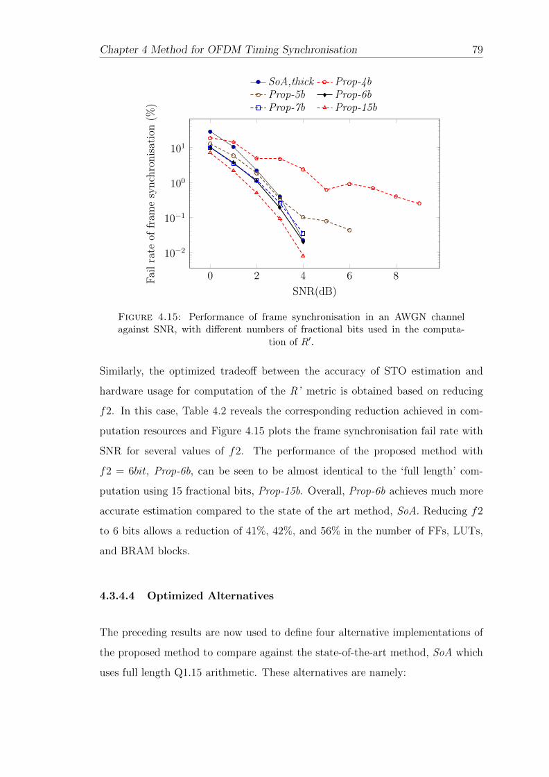
Chapter 4 Method for OFDM Timing Synchronisation 79
0 2 4 6 8
10−2
10−1
100
101
SNR(dB)
Fai
lra
teof
fram
esy
nch
ronis
atio
n(%
)
SoA,thick Prop-4bProp-5b Prop-6bProp-7b Prop-15b
Figure 4.15: Performance of frame synchronisation in an AWGN channelagainst SNR, with different numbers of fractional bits used in the computa-
tion of R′.
Similarly, the optimized tradeoff between the accuracy of STO estimation and
hardware usage for computation of the R’ metric is obtained based on reducing
f2. In this case, Table 4.2 reveals the corresponding reduction achieved in com-
putation resources and Figure 4.15 plots the frame synchronisation fail rate with
SNR for several values of f2. The performance of the proposed method with
f2 = 6bit, Prop-6b, can be seen to be almost identical to the ‘full length’ com-
putation using 15 fractional bits, Prop-15b. Overall, Prop-6b achieves much more
accurate estimation compared to the state of the art method, SoA. Reducing f2
to 6 bits allows a reduction of 41%, 42%, and 56% in the number of FFs, LUTs,
and BRAM blocks.
4.3.4.4 Optimized Alternatives
The preceding results are now used to define four alternative implementations of
the proposed method to compare against the state-of-the-art method, SoA which
uses full length Q1.15 arithmetic. These alternatives are namely:

Chapter 4 Method for OFDM Timing Synchronisation 80
• Prop-A1 : a non-optimized instance of the proposed method with both f1
and f2 set to 15.
• Prop-A2 : only P ′ is optimized with f1 = 7 while f2 remains set to 15.
• Prop-A3 : only R′ is optimized with f2 = 6 while f1 remains set to 15.
• Prop-A4 : both P ′ and R′ are optimized by setting f1 = 7 and f2 = 6.
Table 4.3: Total resources consumed by a full word length implementationof SoA and four reduced complexity instances of the proposed method. Dy-namic (Dpwr) and quiescent power (Qpwr) consumption are reported in mA.
Maximum frequency is reported in MHz.
Slices BRAM DSP Qpwr Dpwr Frequency
SoA 930 112 13 37 41 121
Prop-A1 1000 118 14 37 43 133
Prop-A2 923 86 14 37 39 142
Prop-A3 869 109 14 37 38 137
Prop-A4 777 77 14 37 35 142
Table 4.3 reports the overall hardware resources required for these instances of
the synchroniser, as well as detailing the power consumption of each. It should be
noted that the CFO estimation and frame synchronisation performance of these
instances can be seen by choosing the corresponding word length from plots of P’
& R’ in Figs. 4.14 & 4.15 respectively. In other words, all instances have been
simulated and reported in the previous plots. From the table, it is evident that
reducing word length can yield a significant reduction in both hardware require-
ment and power consumption. The fully optimized alternative, Prop-A4, achieves
a reduction of 16.4%, 31.2%, and 14.6% in the number of occupied slices, BRAMs,
and in dynamic power consumption, when compared to SoA. The maximum fre-
quencies of the SoA and proposed method implementations are also reported. The
required frequency for baseband processing in IEEE 802.16 ranges from from 5.6
to 22.4 MHz, and this requirement is easily met by all tested implementations.

Chapter 4 Method for OFDM Timing Synchronisation 81
Table 5.1 details the comparison between SoA and Prop-A4 in terms of their
constituent building block resources (where the function names in this table cor-
respond to the block diagrams of Figs. 4.11 and 4.12).
Table 4.4: Resource comparison between two synchronisation methods.
Function FF LUT BRAM DSP
SoA |P | metric 303 427 64 3
R metric 168 186 16 2
CFO comp 1478 1517 0 8
Coarse time 7 33 0 0
Fine time 942 1009 32 0
Total 2898 3172 112 13
Prop-A4 |P ′| metric 240 323 64 3
R′ metric 818 600 7 2
CFO comp 1467 1515 0 8
Time sync 66 98 6 1
Total 2591 2536 77 14
The function named ‘CFO comp’, which performs frequency offset estimation and
compensation, clearly consumes the largest amount of hardware in both methods.
The R’ metric computation in Prop-A4 uses more hardware than the computation
of R in SoA. However, fine timing estimation, ‘Fine time’, takes a large proportion
of the total hardware cost in SoA while the alternative in the proposed method
(timing synchronisation, known as ‘Time sync’), requires much less hardware.
4.4 Summary
Although the state of the art synchronisation methods achieve good performance
when the CFO is in the range of fractional CFO estimation, they can not work
with larger CFO. Some methods employ cross-correlation for the time synchroni-
sation; these methods are robust to large CFO and can obtain acceptable perfor-
mance at low SNR. However, the much higher computational resources needed for

Chapter 4 Method for OFDM Timing Synchronisation 82
cross-correlation tend to make such methods unsuitable for hardware implemen-
tation. The methods have been presented to improve upon these drawbacks of
previous reported works. The method takes the advantage of period and energy
distribution characteristics of the preamble to perform time synchronisation. The
synchronisation performance results, obtained through simulation, demonstrate
good performance and robustness to large CFO. Although the method just esti-
mates and compensates the fractional CFO, the method still performs well with
larger CFO values. An enhanced OFDM synchronisation method that provides
an efficient and low cost IFO estimation will be presented in the next chapter.
Chapter 5
IFO Estimation Method for
OFDM Frequency
Synchronisation
5.1 Introduction
In the previous chapter, robust OFDM timing synchronisation was explored, lead-
ing to a proposed method that is able to perform well even in the case of large
fractional CFO. However, the CFO estimation of that method was only estimate
the fractional CFO rather than large integer CFO that can occur as a result of
the Doppler Effect and/or due to local oscillator instabilities. CFO is usually nor-
malised by subcarrier spacing and divided into an integer frequency offset (IFO)
part, which is a whole multiple of subcarrier spacings, and a remainder which
is referred to as fractional frequency offset (FFO). IFO causes a circular shift of
the subcarrier in the frequency domain while FFO results in ICI because of lost
orthogonality between subcarriers. Figure 5.1 illustrates the process of FFO and
IFO estimation in the baseband processing of a typical OFDM system. The IFO
estimation is performed after the FFT, and relies upon cross-correlation, which
consumes significant hardware resources. A typical OFDM receiver avoids the
83

Chapter 5 IFO Estimation Method for OFDM Frequency Synchronisation 84
need for IFO estimation by limiting CFO tolerance to be smaller than the range
of allowable FFO estimation, resulting in a set of very strict constraints on the
design of the RF front-end. However, if CFO exceeds the range of FFO estima-
tion, IFO is present and the system cannot therefore function correctly. This is
more pronounced in applications that subject the front-end to intensive Doppler
(including rapidly mobile systems), for very high carrier frequencies, or systems
which aim to support multiple frequency bands for different standards.
In this chapter, a novel method is proposed for IFO estimation to overcome this
challenge to efficient and low-power implementation. The basis of this method has
also been discussed in:
• T. H. Pham, S. A. Fahmy, and I. V. McLoughlin, “Efficient Integer Frequency
Offset Estimation Architecture for Enhanced OFDM Synchronisation,” in
IEEE Transactions on Very Large Scale Integration (VLSI) Systems, vol.PP,
no.99, pp.1-1, 2015.
5.2 Related Work
As mentioned in the previous chapter, the estimation range of fractional CFO has
a limitation that is shown in (4.8); for instance its range is up to ±2 subcarrier
spacings in the case of the IEEE 802.16 preamble. The value of the IFO is a
multiple of the coarse CFO’s range. It is commonly estimated by performing
cross-correlation [99, 13] in the frequency domain.
Figure 5.1: Baseband processing block diagram.

Chapter 5 IFO Estimation Method for OFDM Frequency Synchronisation 85
Let us assume that the signal is transmitted over a frequency selective channel
that has channel impulse response (CIR) h with length, L (L < NCP ), and which
is corrupted by AWGN. The received signal, suffering frequency and timing offsets,
can be expressed in the time domain as
y[n] =L−1∑l=0
h[l]x[n− τ − l]ei(2πξ n−τN +φ0) + w[n] (5.1)
where w[n] denotes AWGN in the time domain, τ , φ0 are residual timing offset
(RTO) and error phase, respectively, and ξ is the normalised CFO that can be
divided into an FFO part λ and an IFO part ε as ξ = λ+ ε.
Assuming FFO and STO be compensated by earlier stages of synchronisation, as
has been investigated in detail by other authors [13, 94], the received preamble
symbol after CP removal at FFT output is
Y [k] = ei(φ0−2π τkN
)H[k − ε]X[k − ε] +W [k] (5.2)
where W [k] and H[k] are the frequency domain representations of AWGN and
CIR, respectively.
As mentioned previously, IFO results in a cyclic shift in the frequency domain and
is commonly estimated by performing cross-correlation in the frequency domain.
By contrast, RTO causes a linear phase rotation on samples in the frequency
domain that may cause degradation of cross-correlation performance during IFO
estimation. Based on a differential demodulation of the FFT output, the IFO
can be determined with better robustness to frequency selective channel and RTO
effects using the correlation function [100] expressed by:
ε = argmaxε
∣∣∣∣∣N∑k=1
Y ∗[k − 1]Y [k]X∗[k − ε]X[k − 1− ε]∣∣∣∣∣ (5.3)
where (.)∗ denotes complex conjugation, ε, ε are estimated and trial values of ε,
respectively, Y [k] and X[k] denote the kth frequency symbol index of the received

Chapter 5 IFO Estimation Method for OFDM Frequency Synchronisation 86
symbol and the known transmitted preamble, respectively, and the symbol size N
is equal to the FFT size.
The estimated IFO can achieve high precision using cross-correlation in the fre-
quency domain, however implementing cross-correlation clearly involves a signif-
icant hardware overhead, with a multiplier needed for each element in the cross-
correlation. Sign-bit cross-correlation [95] is a widely adopted approach to reduc-
ing correlation complexity using only the most significant bit (MSB) of the signed
two’s complement numbers in the correlation computation. In this way, complex-
ity is reduced at the cost of some performance degradation. Despite the adoption
of such methods, cross-correlation remains computationally expensive, especially
when dealing with a large FFT size. It should be noted here that several IFO
estimation methods have been published which claim robustness to frequency se-
lective channels and RTO. However, published FPGA implementations of these
methods are lacking to date, possibly because the hardware costs are considerable
– even when adopting the sign-bit cross-correlation approach as mentioned.
There are few practical implementations for IFO estimation and correction. A
notable exception was presented in [13], in which time-domain cross correlation is
performed between received samples and several pre-rotated versions of the pream-
ble corresponding to possible IFO values. Although this method uses efficient
sign-bit correlation to reduce hardware cost (at the cost of decreased estimation
accuracy and increased sensitive to frequency selective channels), it is not efficient
when the possible IFO range is large since it effectively performs an exhaustive
search of possibilities.
State of the art OFDM synchronisation methods typically have a small tolerance
of CFO that requires the hardware be strictly constrained to ensure operation
within a small CFO range which does not include any IFO. This strict timing
requirement leads to an increase in total system cost. Particularly, in the case
of accessing multiple frequency bands for different standards, the need for high
precision timing, coupled with a requirement for a wide ranging and agile operating
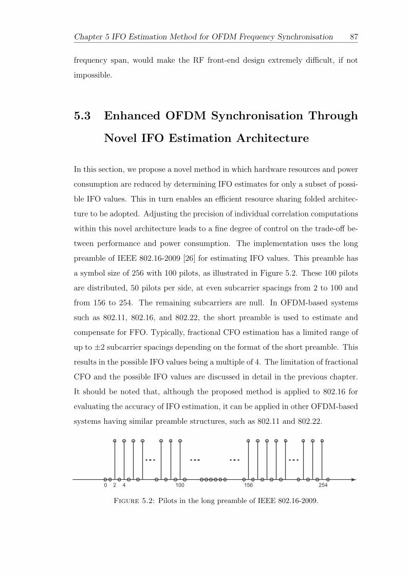
Chapter 5 IFO Estimation Method for OFDM Frequency Synchronisation 87
frequency span, would make the RF front-end design extremely difficult, if not
impossible.
5.3 Enhanced OFDM Synchronisation Through
Novel IFO Estimation Architecture
In this section, we propose a novel method in which hardware resources and power
consumption are reduced by determining IFO estimates for only a subset of possi-
ble IFO values. This in turn enables an efficient resource sharing folded architec-
ture to be adopted. Adjusting the precision of individual correlation computations
within this novel architecture leads to a fine degree of control on the trade-off be-
tween performance and power consumption. The implementation uses the long
preamble of IEEE 802.16-2009 [26] for estimating IFO values. This preamble has
a symbol size of 256 with 100 pilots, as illustrated in Figure 5.2. These 100 pilots
are distributed, 50 pilots per side, at even subcarrier spacings from 2 to 100 and
from 156 to 254. The remaining subcarriers are null. In OFDM-based systems
such as 802.11, 802.16, and 802.22, the short preamble is used to estimate and
compensate for FFO. Typically, fractional CFO estimation has a limited range of
up to ±2 subcarrier spacings depending on the format of the short preamble. This
results in the possible IFO values being a multiple of 4. The limitation of fractional
CFO and the possible IFO values are discussed in detail in the previous chapter.
It should be noted that, although the proposed method is applied to 802.16 for
evaluating the accuracy of IFO estimation, it can be applied in other OFDM-based
systems having similar preamble structures, such as 802.11 and 802.22.
Figure 5.2: Pilots in the long preamble of IEEE 802.16-2009.

Chapter 5 IFO Estimation Method for OFDM Frequency Synchronisation 88
5.3.1 Proposed Algorithm
Firstly, a subset of possible IFO values is determined. We assume that the RF
front end can provide CFO stability in a range from -14 to +18 subcarrier spacings,
which is relaxed compared to the strict RF front end constraints in 802.16 that
would typically otherwise lead to increased RF hardware costs. Generally, the
larger the range of IFO estimation that is performed, the larger the CFO that the
baseband system can tolerate. A wider CFO tolerance in turn leads to a relaxation
in RF front-end specification, hence reducing system cost. In this system, there
are 8 possible values for IFO estimation in the assumed CFO range. The subset
of possible IFO values is denoted SIFO = {−12,−8,−4, 0, 4, 8, 12, 16}. Moreover,
samples are pre-offset by 12 subcarrier spacings prior to calculation to ensure that
all possible values of IFO are positive, S ′IFO = {0 : 4 : 28}. This means that
received symbols will only ever need to be shifted right to compensate IFO, thus
reducing buffer memory requirements.
Secondly, a resource sharing folded architecture is designed to significantly reduce
the hardware cost. Conventionally, to obtain high accuracy, IFO estimation is
computed across all pilots in the preamble. This results in considerable hardware
overhead, especially with a large number of pilots, as is the case for IEEE 802.16-
2009. Evidently, as the number of pilots increases, the correlation result shows
greater robustness to noise. However, we will demonstrate in Section 5.3.3 that the
beneficial effect of calculating across additional pilots leads to decreasing gains in
performance. In fact the performance improvement reaches a plateau. We there-
fore propose making use of only a subset of pilots, while maintaining estimation
accuracy as much as possible. Then, by spreading the chosen subset of pilots
carefully in the time domain, it becomes possible to design a resource-sharing
architecture for computing the cross-correlation, hence reducing area and power
consumption. When the proposed method is applied to IEEE 802.16-2009 offset
estimation, the pilots used for the IFO computation are selected at subcarrier
indices that are multiples of 4, leading to a natural four-fold resource sharing

Chapter 5 IFO Estimation Method for OFDM Frequency Synchronisation 89
architecture. Hence, the IFO estimation can be expressed as:
ε = argmaxε∈S′IFO
∣∣∣∣∣∣N/4∑k=1
P (4k)A(4k − ε)
∣∣∣∣∣∣ (5.4)
where P (4k) = Y ∗(4k − 2)Y (4k) denotes the correlation of two consecutive re-
ceived pilots, and A(4k) = X(4k − 2)X∗(4k) is the correlation of two consecutive
transmitted pilots that can be pre-computed.
Thirdly, although sign-bit cross-correlation is often used in conventional imple-
mentations [13, 95], as it can significantly reduce computational complexity, it
also leads to reduced precision and hence reduced estimation performance, espe-
cially in the case of frequency selective channels. For this reason, we instead apply
multiplierless correlation to enhance the accuracy of estimation (i.e. using several
bits for computation, rather than the existing extremes of either a single sign bit or
a full word computation). In [98], we demonstrated a trade-off between cost and
accuracy for multiplierless OFDM synchronisation. We further investigate this
effect in the current chapter in terms of the trade-off between cost and accuracy
when reducing the wordlength used to represent P (4k).
5.3.2 Proposed Architecture
The proposed method divides IFO estimation into multiple repeated computations
with resource sharing based upon the four-sample timing between selected spread
pilots. The estimation of IFO in (7.4) can now be rewritten as follows:
ε = argmaxε∈S′IFO
|Vε| ,
Vε =25∑k=0
P (4k)Aε(4k) + P (L+ 4k)Aε(L+ 4k), (5.5)
where Aε denotes the correlation of two consecutive pre-rotated known pilots cor-
responding to one IFO value, and Vε is the cross-correlation between received pilots
and pre-rotated known pilots. Since the pilots of the long preamble are distributed

Chapter 5 IFO Estimation Method for OFDM Frequency Synchronisation 90
Figure 5.3: Circuit for the known-pilots shift register.
on two sides of the OFDM symbol in the frequency domain, at even subcarrier
spacings from 2 to 100 and 156 to 254, L denotes the index of the first pilots in
second half. In the case of IEEE 802.16, L equals 156. Each value, Vε, can be
computed simultaneously and separately using a multi-add accumulation scheme.
The challenge in implementation is to find a way to efficiently share resources
when computing Vε. The pilots that are used to compute the correlation arrive
every four cycles so there are four spare cycles between two consecutive computed
pilots, allowing one multiply accumulate block to sequentially compute 4 separate
correlations.
There are 8 sets of Aε corresponding to 8 possible IFOs. These sets of Aε can be
pre-computed and stored separately. Due to the spreading of the computed pilots,
the Aε sets have many identical pilots – this naturally allows sharing between
pre-rotated pilot sets – so that only 64 memory locations are required instead of
400. Thus, an 84% reduction in the memory used to store Aε sets is achieved.
Figure 5.3 illustrates the Aε sets and circuitry for combining all Aε sets.
Multiply accumulate blocks are shared for computing four sequential Vε values
over four successive clock periods. Figure 5.4 demonstrates how this is done. Pk
is received in every clock cycle. P4k is the subsampling of Pk, taking a subset
of the most significant bits from Pk every four cycles. The cross-correlation is
performed with the values of P4k. Two multipliers, M1 and M2 are used to
compute the values of 8 cross-correlations Vε in parallel. Each multiplier performs
multiplications sequentially between P4k and the corresponding transmitted pilots
in 4 sets of Aε. The products are accumulated to the values of Vε. When all pilots

Chapter 5 IFO Estimation Method for OFDM Frequency Synchronisation 91
Figure 5.4: Resource sharing approach for computing Vε.
are computed, the maximum operation, argmax|V |, is performed on 8 Vε values
to estimate the IFO.
To design an optimised architecture for IFO estimation, the multiply-add formula
of Vε is mathematically manipulated into what is effectively a multiply-accumulate
form. When one received sample is taken, Vε can be expressed in the form of
accumulations as follows:
Vε(n) = Aε(n)P (n) + Vε(n− 1),
= (<{CA} − i={CA})(<{P (n)}+ i={P (n)})
+(<{Vε(n− 1)}+ i={Vε(n− 1)}) (5.6)
where <{.} and ={.} denote the real and imaginary parts, respectively, and P(n),
Aε(n) denote the current values of the correlation of two consecutive received pilots
and corresponding transmitted pilots, respectively. Vε(n − 1) is the accumulated

Chapter 5 IFO Estimation Method for OFDM Frequency Synchronisation 92
Figure 5.5: Architecture of proposed IFO estimator.
value of Vε. To employ multiplierless correlation, Aε are normalized to values CA
whose real and imaginary parts have values in {-1, 0, 1}, and the wordlength of
P(n) and Vε in fixed point format can be adjusted to increase estimation accuracy
at the cost of increased hardware resource consumption. The real and imaginary
parts of Vε can then be computed as
<{Vε(n)} = <{CA}<{P (n)}+ ={CA}={P (n)}
+<{Vε(n− 1)},
={Vε(n)} = <{CA}={P (n)} − ={CA}<{P (n)}
+={Vε(n− 1)} (5.7)

Chapter 5 IFO Estimation Method for OFDM Frequency Synchronisation 93
The proposed resource sharing architecture for the IFO estimator is shown in Fig-
ure 5.5. The ArgMax module finds the maximum of the 8 Vε values in order to
identify the corresponding IFO estimate. The novelty of this IFO estimator is in
terms of algorithmic improvements and architecture optimisation. This is achieved
by firstly reformulating the equation into an expression that is computable with
efficient shared resource circuitry. Because of the significant hardware reduction
achieved, this IFO estimator can be feasibly implemented on a low-power, lim-
ited hardware resource FPGA, while simultaneously ensuring that performance is
maintained by a trade off between number of pilots against word length.
We are able to demonstrate that the algorithm and structure optimisations men-
tioned above retain competitive estimation accuracy compared to conventional
approaches, while also offering significant reductions in hardware resource usage.
This makes it possible to implement a high-performance OFDM receiver on a
low-power FPGA, especially where the available number of DSP blocks is limited.
5.3.3 Simulation
Many variants of the proposed method were simulated in MATLAB using different
channel models and the parameter set of the IEEE 802.16-2009 downlink preamble.
Performance of the implementation was compared to the theoretical performance
of some state of the art methods. This was assessed primarily in terms of the prob-
ability of failed estimation (POFE) with respect to channel SNR. POFE, which is
widely used to evaluate the performance of IFO estimation [100, 43, 44], measures
the number of fail estimations divided by the total number of IFO estimations.
Overall, 100,000 IFO estimations were simulated in AWGN and Stanford Univer-
sity Interim (SUI) [97] frequency selective channels. IFO estimation is performed
with non-ideal FFO compensation, and FFO is determined and compensated using
the method of Kim and Park [13]. The simulation also verifies the performance of
the proposed method under the effect of RTO caused by imperfect STO estimation
(assuming that STO estimation is still within the CP and does not cause ISI). In

Chapter 5 IFO Estimation Method for OFDM Frequency Synchronisation 94
addition, a randomly generated amount of STO is added in the range from 0 to
NCP − L− 1, where L is the length of CIR.
We first investigate the performance degradation compared to theoretical perfor-
mance as a result of reducing the number of pilots as proposed. Next, we will
investigate the effect of wordlength optimisation. In both cases, comparisons are
made with established methods in the literature that can be simulated but are oth-
erwise infeasible for hardware implementation, namely the conventional method
in [100] (PCH ) that is applied to one training block with 100 pilots. In addition,
two state of the art methods are also simulated for comparison. Firstly, metric SY
from [43] as defined by,
ε = argmaxε∈SIFO
|µSY
(ε)| ,
µSY
(ε) = <
N2∑
k=1
Y ∗(2k−2)Y(2k)X∗(2k−ε)X(2k−2−ε)
(5.8)
Secondly, metric MM from [44],
ε = argmaxε∈SIFO
|µMM
(ε)| ,
µMM
(ε) = <
eiπ4N2∑
k=1
Y ∗(2k−2)Y(2k)X∗(2k−ε)X(2k−2−ε)
(5.9)
where <{.} denotes the real part.
We are unaware of any published circuits for these methods, because of their
complex computation. The very large hardware requirement for these respective
metrics does not lend either method to feasible implementation on a low cost, low
power FPGA (unlike the proposed method).

Chapter 5 IFO Estimation Method for OFDM Frequency Synchronisation 95
5.3.3.1 Performance Comparison
The performance of the proposed method, denoted Prop, is evaluated in com-
parison to the theoretical performance of state of the art methods by Park et.
al. [100], Shim and You [43] and Morelli and Moretti [44], denoted PCH, SY and
MM, respectively in the previous subsection. The theoretical performance is com-
puted with full precision using full multiplication. However, it must be noted
that implementing this directly in hardware would be prohibitive due to the large
number of multiplication operations needed. In fact, hardware implementation
would conventionally use sign-bit correlation instead of full precision correlation,
as mentioned previously. Thus the full multiplication results shown here are un-
doubtedly better than those achievable in practice, and thus can be considered as
upper performance bounds. For more realistic data, we also provide results from
sign-bit correlation versions of the above, denoted PCH sb, SY sb, and MM sb
respectively.
The proposed method, evaluated against these, uses 50 spread pilots with indices
that are multiples of 4. For the sake of comparison, an additional implementation
of PCH is reported which, like the proposed method, uses only 50 pilots, but
which are placed continuously rather than being spread. This is denoted PCH 50.
Figs. 5.6 and 5.7 plot performance results for all methods in an AWGN channel,
with and without RTO respectively, and reveal that the proposed method gener-
ally performs well, especially at higher SNRs. Considering more realistic channel
models, Figs. 5.8 and 5.9 plot the performance of all methods in SUI1, and SUI2
channels respectively, and similarly show that the proposed method performs well,
especially at higher SNRs.
Under these experimental conditions, PCH and SY achieve equivalent perfor-
mance in AWGN without RTO and in SUI1 channels. However, SY degrades
more drastically than PCH in the SUI2 channel at SNRs above 1 dB. SY also
deteriorates in the case of AWGN with RTO. This method appears to be very sen-
sitive to large RTO, while MM and PCH exhibit better robustness to RTO. The
accuracy of MM is slightly lower than that of PCH at SNRs below 0 dB, while

Chapter 5 IFO Estimation Method for OFDM Frequency Synchronisation 96
−6 −4 −2 0 2 4 6 8 10 1210−3
10−2
10−1
100
101
102
SNR(dB)
Pro
bab
ilit
yof
Fai
lE
stim
atio
n(%
)
MM MM sb SY SY sbPCH PCH sb PCH 50 Prop
Figure 5.6: Fail rate of IFO estimation methods in AWGN channel withoutRTO.
−6 −4 −2 0 2 4 6 8 10 1210−3
10−2
10−1
100
101
102
SNR(dB)
Pro
bab
ilit
yof
Fai
lE
stim
atio
n(%
)
MM MM sb SY SY sbPCH PCH sb PCH 50 Prop
Figure 5.7: Fail rate of IFO estimation methods in AWGN channel with RTO.

Chapter 5 IFO Estimation Method for OFDM Frequency Synchronisation 97
−6 −4 −2 0 2 4 6 8 10 1210−3
10−2
10−1
100
101
102
SNR(dB)
Pro
bab
ilit
yof
Fai
lE
stim
atio
n(%
)
MM MM sb SY SY sbPCH PCH sb PCH 50 Prop
Figure 5.8: Fail rate of IFO estimation methods in SUI1 channel.
−6 −4 −2 0 2 4 6 8 10 1210−3
10−2
10−1
100
101
102
SNR(dB)
Pro
bab
ilit
yof
Fai
lE
stim
atio
n(%
)
MM MM sb SY SY sbPCH PCH sb PCH 50 Prop
Figure 5.9: Fail rate of IFO estimation methods in SUI2 channel.

Chapter 5 IFO Estimation Method for OFDM Frequency Synchronisation 98
performance is very similar at larger SNRs. Also note the performance of the
conventional approach implementations, PCH sb, SY sb, MM sb which degrade
significantly with SNR, especially in the SUI1, SUI2 channels.
Apart from at very low SNRs, the proposed method, Prop, achieves almost iden-
tical performance to the simulated upper bound PCH, even in the presence of
RTO. It should be noted that Prop achieves this while allowing the use of resource
sharing through sparse pilot computation. This will be used below to achieve a
significant hardware saving. According to simulation results, Prop, with its spread
pilots, is also more accurate than PCH 50 that uses the same number of pilots,
but places them continuously.
5.3.3.2 Wordlength Optimisation
Since sign-bit correlation degrades IFO estimation performance, specially in fre-
quency selective channels, the proposed method instead employs multiplierless
correlation to improve accuracy and robustness. The complexity of this approach
is dependent on the wordlength chosen for the correlation computation. We now
investigate how wordlength affects the performance of the proposed implementa-
tion, again compared to the theoretical bound, PCH, as well as to the performance
of a conventional sign-bit implementation, PCH sb. We denote wordlength using
the notation Q1.f , meaning a single integer bit and f fractional bits. Evaluations
are performed for f of 1, 2, 7, and 15 bits. These results will be plotted in the
following figures with the labels Prop 1b, Prop 2b, Prop 7b, and Prop 15b, respec-
tively. Figs. 5.10 and 5.11 plot the performance in AWGN (with and without
RTO), with all tested wordlengths in the proposed method performing compara-
bly to PCH (and being much better than PCH sb at SNRs exceeding about 2 dB).
Figs. 5.12 and 5.13 plot the results when using the more realistic SUI1 and SUI2
channel models.
It can be seen from the plots that each of the tested wordlengths achieves much
better performance and exhibits greater robustness to frequency selective channels
than the sign-bit realisation of the conventional approach, PCH sb. Additionally,

Chapter 5 IFO Estimation Method for OFDM Frequency Synchronisation 99
−6 −4 −2 0 2 4 6 8 10 1210−3
10−2
10−1
100
101
102
SNR(dB)
Pro
bab
ilit
yof
Fai
lE
stim
atio
n(%
)
PCH PCH sb Prop 15bProp 7b Prop 2b Prop 1b
Figure 5.10: Fail rate for different wordlengths in AWGN channel withoutRTO.
−6 −4 −2 0 2 4 6 8 10 1210−3
10−2
10−1
100
101
102
SNR(dB)
Pro
bab
ilit
yof
Fai
lE
stim
atio
n(%
)
PCH PCH sb Prop 15bProp 7b Prop 2b Prop 1b
Figure 5.11: Fail rate for different wordlengths in AWGN channel with RTO.

Chapter 5 IFO Estimation Method for OFDM Frequency Synchronisation 100
−6 −4 −2 0 2 4 6 8 10 1210−3
10−2
10−1
100
101
102
SNR(dB)
Pro
bab
ilit
yof
Fai
lE
stim
atio
n(%
)
PCH PCH sb Prop 15bProp 7b Prop 2b Prop 1b
Figure 5.12: Fail rate for different wordlengths in SUI1 channel.
−6 −4 −2 0 2 4 6 8 10 1210−3
10−2
10−1
100
101
102
SNR(dB)
Pro
bab
ilit
yof
Fai
lE
stim
atio
n(%
)
PCH PCH sb Prop 15bProp 7b Prop 2b Prop 1b
Figure 5.13: Fail rate for different wordlengths in SUI2 channel.

Chapter 5 IFO Estimation Method for OFDM Frequency Synchronisation 101
these realisations of the proposed method do not suffer as much degradation in
the presence of RTO. Moreover, it is possible to improve low SNR performance
by adopting a longer wordlength with the proposed method, at a cost of increased
hardware complexity. Increasing wordlength does improve results slightly, with
the step from 1 to 2 bits being the most significant gain. By contrast, increasing
from 2 to 7 or from 7 to 15 bits has little impact. In general, Prop 2b achieves
an estimation accuracy close to that of the theoretical performance bound, PCH,
at intermediate and higher SNRs, even though it involves computation with fewer
bits, and can hence be implemented more efficiently.
5.3.4 FPGA Implementation
The analysis in Section 5.3.3 suggests that the proposed method offers comparable
estimation performance to existing methods in the literature. As a result of the
simplifications inherent in the proposed approach, this should be achievable at
a reduced hardware cost. This section now quantifies this hardware cost, for an
FPGA-based implementation. It is important to note that these hardware savings
are accessible for a number of target implementation devices, although we are
interested primarily in FPGA implementation as part of our work on leveraging
FPGA reconfigurability in cognitive radios.
5.3.4.1 Conventional Approach
To obtain the theoretical performance previously discussed in Section 5.3.3 and
denoted as PCH, the computation of the estimation metric in [100], using 100
pilots, would require about 200 complex multipliers, resulting in the use of over
600 DSP blocks. This may exceed the available resources on small devices, or
leave insufficient resources for other tasks on larger devices. As the number of
multiplications required for a full implementation of the approach is prohibitive,
the conventional approach for implementation, as we have discussed, uses sign-bit
correlation [13]. This conventional implementation uses all 100 pilots in the long

Chapter 5 IFO Estimation Method for OFDM Frequency Synchronisation 102
Figure 5.14: DSP block based 3-input adder for correlation.
preamble to perform sign-bit correlation, and multiply adds are eliminated at taps
where the pilots of the long preamble are not used. This implementation mirrors
the PCH sb in Section 5.3.3, and allows us to quantify the benefits of our proposed
approach against a known reference benchmark.
5.3.4.2 Proposed Approach
The proposed architecture for the IFO estimator, implemented with several differ-
ent wordlengths of P (n) and Vε in (5.6), are compared to allow us to explore the
hardware costs associated with the respective implementations. Four fixed point
formats for P (n), are investigated: Q1.1, Q1.2, Q1.7, and Q1.15. Vε is represented
accordingly in Q7.1, Q7.2, Q7.7, and Q7.15 formats to avoid overflow.
In order to obtain a comprehensive optimised implementation, these circuits are
each implemented using two different structures. The first uses only logic elements
(LE) for computation, while the second uses Xilinx DSP48A1 [101] primitives.
Considering (5.7), <{Vε(n)},={Vε(n)} can be computed effectively using two DSP
blocks as 3-input adders, instead of 4 blocks as would be usual. Figure 5.14
illustrates how this is done for <{Vε(n)}, and similarly for ={Vε(n)}. Note that
the solution presented in Figure 5.14 is optimised for QPSK modulated pilots
(since their amplitudes are identical) as specified in IEEE 802.16, as well as in
most OFDM-based standards. The normalisation performed in (5.7) allows the
correlation to be reduced to two DSP blocks operating as 3-input adders (instead

Chapter 5 IFO Estimation Method for OFDM Frequency Synchronisation 103
of 4 DSP blocks with multipliers as would be usual). These methods correspond
to Prop 1b, Prop 2b, Prop 7b, and Prop 15b that were investigated for estimation
accuracy in Section 5.3.3.
5.3.5 Implementation Results
The circuits were synthesised and fully implemented using Xilinx ISE 13.2, target-
ing the low-power Xilinx Spartan-6 XC6SLX75T FPGA. The results are reported
in terms of the number of flip-flops (FF), look-up tables (LUT), and DSP48 blocks,
along with dynamic power consumption, as summarised in Table 5.1.
Table 5.1: Resource utilisation and dynamic power of IFO estimators.
IFO est. Cir. #FF #LUT #DSP Fre (MHz) D. Power
conv 100p 3270 (3%) 1837 (3%) 3 142 42 mW
Prop 1b LE 328 (1%) 370 (1%) 3 136 9 mW
Prop 2b LE 350 (1%) 390 (1%) 3 136 10 mW
Prop 7b LE 460 (1%) 471 (1%) 3 136 12 mW
Prop 15b LE 735 (1%) 696 (1%) 3 134 17 mW
Prop 1b DSP 328 (1%) 306 (1%) 7 78 11 mW
Prop 2b DSP 350 (1%) 319 (1%) 7 78 12 mW
Prop 7b DSP 460 (1%) 379 (1%) 7 77 14 mW
Prop 15b DSP 735 (1%) 591 (1%) 7 77 18 mW
conv 100p refers to the conventional approach, implemented using sign-bit corre-
lation over 100 pilots. Prop fb LE, Prop fb DSP, in which f = 1, 2, 7 and 15 (cor-
responding to received sample format Q1.f), denote the circuits of corresponding
wordlengths, implemented using logic elements and DSP48 blocks, respectively.
Referring to the table, the proposed implementation shows that significant im-
provement in resource usage and dynamic power consumption is possible with the
proposed method.
The hardware resources used by Prop fb LE and Prop fb DSP increase gradu-
ally, in terms of FFs and LUTs, as the wordlength increases. The number of
FFs used in Prop fb DSP and Prop fb LE is equal, while Prop fb DSP uses fewer

Chapter 5 IFO Estimation Method for OFDM Frequency Synchronisation 104
LUTs since the DSP blocks are used for the 3-input additions. The Prop fb LE
implementations use 3 DSP blocks to compute P (n), while Prop fb DSP require
an additional 4 DSP blocks to perform the correlation. Prop fb LE, Prop fb DSP
both consume far fewer LUT and FF resources than the conventional conv 100p
implementation. For Prop 2b LE, the number of FFs and LUTs is reduced by 90%
and 79% respectively compared to the conventional conv 100p approach.
The maximum frequencies of the various circuits, reported after place and route,
comfortably exceed the timing requirements for IEEE 802.16 synchronisation whose
sampling frequency is below 25 MHz. A post-place-and-route simulation was used
to estimate the power consumption of the system at a clock rate of 50 MHz, using
the Xilinx XPower tool – also shown in table 5.1. Prop fb LE implementations
consume less power than the equivalent Prop fb DSP implementations. All im-
plementations of the proposed method consume significantly less power than the
conventional implementation. Prop 2b LE consumes just 22% of the power con-
sumed by conv 100p.
In subsection 5.3.3, we established that Prop 2b LE easily outperforms the con-
ventional approach in terms of estimation accuracy. In this subsection, we have
shown that it does so with a significant hardware resource saving, and with sig-
nificantly reduced power consumption. In fact, the estimation performance of
Prop 2b LE, in AWGN and SUI channels (except at very low SNR), is close to the
theoretical bound of PCH, which would demand a significant proportion of the
FPGAs resources if it were implemented conventionally. Meanwhile, Prop 2b LE
is extremely efficient, consuming less than 1% of the resources available on a
low-power Spartan-6 XC6SLX75 FPGA. Beyond IEEE 802.16-2009, the folded re-
source sharing architecture, which leverages sub-sample spaced OFDM pilots, can
be adopted for use in other OFDM standards (including IEEE 802.11 and IEEE
802.22).

Chapter 5 IFO Estimation Method for OFDM Frequency Synchronisation 105
5.4 Summary
This chapter investigated IFO estimation in OFDM-based systems such as IEEE
802.16. A technique is proposed for efficient implementation of IFO estimation,
which aims in particular for a low power and low resource utilisation. Since IFO
estimation contributes significantly to the complexity of a robust synchroniser
design, this work is important for multistandard radios, or applications where sig-
nificant frequency variation is expected. Robust IFO estimation allows for relaxed
analogue RF constraints, leading to reduced cost. A modified timing metric is
derived which allows for resource sharing to reduce both resource requirements
as well as power consumption. The proposed implementation makes use of a
four-fold resource sharing architecture to significantly reduce hardware cost, while
multiplierless correlation with optimised wordlength is used to improve estimation
accuracy in comparison to a conventional implementation approach using signbit
correlation. The method is shown to perform as well as current state-of-the-art
methods that employ multiplier-based correlation, and yet with significantly im-
proved power and resource requirements. Dynamic power consumption is reduced
by 78% over even a sign-bit version of the conventional approach, yet it offers
better estimation performance in both AWGN and frequency selective channels.
Beyond IEEE 802.16-2009, the folded resource sharing method, which leverages
sub-sample spaced OFDM pilots, can be adopted for use in other OFDM stan-
dards (including IEEE 802.11 and IEEE 802.22). Multiplierless correlation with
word length optimisation is already used within communication systems, however
the trade off between the number of pilots and computational accuracy for timing
synchronisation is relatively unexplored in the research literature to date.

Chapter 6
Spectrum Efficient Shaping
Method for OFDM Cognitive
Radios
6.1 Introduction
This chapter is concerned with the OFDM spectral leakage challenge for OFDM-
based CRs. OFDM signals typically cause large amounts of spectral leakage,
whereas CRs demand a shaped spectrum confined within the allocated channel
in order to reuse free spectral bands without causing ICI to other users occupy-
ing adjacent bands. Some recent OFDM-based standards are defined with the
requirements on spectral leakage that are extremely stringent in an effort to avoid
ICI. Spectral leakage filtering may cause some effects on transmitted signals that
lead to a reduction in the effective timing guard. Therefore, the implementations
of spectral leakage filtering need to be able to take into account the parameters
of the underlying OFDM signal and its channel characteristics to avoid causing
negative effects on the transmitted signal such as distortion and ISI.
In this chapter, a novel method that embeds baseband filtering within a cognitive
radio (CR) architecture, is proposed. The method is able to meet the specification
106

Chapter 6 Spectrum Efficient Shaping Method for OFDM Cognitive Radios 107
for the most stringent 802.11p SEM, meet the specification of the 802.11af strict
SEM requirement, and furthermore can allow ten additional 802.11af subcarriers
to occupy a single basic channel without violating SEM specifications. In addition,
the method can adaptively change filter performance according to the transmission
power to reduce computational cost while guaranteeing that the emission spectrum
remains smaller than the allowed spectral leakage. The method, performed at
baseband, relaxes otherwise strict RF front-end requirements. This allows the RF
subsystem to be implemented using much less stringent 802.11a designs, which
can significantly reduce total cost.
The work presented in this chapter has also been discussed in:
• T. H. Pham, I. V. McLoughlin, and S. A. Fahmy, “Shaping Spectral Leakage
for IEEE 802.11p Vehicular Communications,” in Proceedings of IEEE Ve-
hicular Technology Conference (VTC Spring), Seoul, Korea, May 2014 [16].
• T. H. Pham, S. A. Fahmy, and I. V. McLoughlin, “Spectrally Efficient Emis-
sion Mask Shaping for OFDM Cognitive Radios,” under review for Digital
Signal Processing.
6.2 Signal Model for Spectral Leakage Filtering
Conventionally, there are two methods that can be employed to compress the spec-
tral leakage for OFDM-based system, namely pulse shaping and image spectrum
compression. Pulse shaping, recommended in 802.11a, is effective at reducing side
lobes. Spectral leakage filtering is designed with respect to the signal model and
channel model to avoid the negative effects of filtering. In this section, we present
the OFDM signal model and 802.11p and 802.11af channel models for compressing
the spectral leakage.

Chapter 6 Spectrum Efficient Shaping Method for OFDM Cognitive Radios 108
6.2.1 Signal Model
We define an OFDM symbol to have inverse fast Fourier transform (IFFT) length
and cyclic prefix (CP) length N and NCP , respectively, so that the length of the
symbol including its CP is NT = N +NCP . A sample x(m) of the OFDM symbol
(0 ≤ m ≤ NT − 1) can be expressed in the time domain as
x(m) =1
N
N−1∑k=0
X(k)ei2πkN
(m−NCP ), (6.1)
where X(k) denotes the frequency domain representation of the data subcarriers.
Since OFDM symbol samples are generally transmitted sequentially, this is equiv-
alent to multiplying symbols with a rectangular window function, p. Then the
transmitted OFDM samples can be expressed as
x(n) =1
N
∞∑l=−∞
N−1∑k=0
X(k)p(n− lNT )ei2πkN
(n−NCP−lNT ). (6.2)
In a conventional OFDM system, the window function, p(m), is rectangular and
simply described as
p(m) =
1, m = 0, 1, ..., NT
0, otherwise
(6.3)
The CIR, of length h, is derived from the delay spread of the channel. If the
CP is shorter than the channel delay, ISI will be present in the received symbols.
Channels experienced by the two standards discussed in this chapter will obviously
differ, but both tend to experience high levels of delay spread: 802.11p because it is
primarily a vehicular communications standard, and 802.11af because it operates
in lower attenuation UHF and VHF bands.
The PHYs specified in 802.11p and 802.11af are largely inherited from the well-
established 802.11a and 802.11ac OFDM PHYs, respectively. The major param-
eters of both new PHYs are presented in Table 6.1. However, since the new

Chapter 6 Spectrum Efficient Shaping Method for OFDM Cognitive Radios 109
standards operate in different channel regions and environments, they are sub-
ject to different, and much more stringent SEM requirements than their parent
standards.
Table 6.1: Major parameters of 802.11p and 802.11af OFDM PHYs
Parameters 802.11p 802.11af
Bandwidth, MHz 10 6 7 8
Used subcarriers, NC 52 114
Total subcarriers, NT 64 144 168 144
FFT points, NFFT 64 128
Subcarrier spacing ∆f , MHz 10/64 6/144 7/168 8/144
Sampling frequency, MHz 10 5.33 5.33 7.11
Fourier transform size 6.4 us 24 us 24 us 18 us
CP length 1.6 us 6 us 6 us 4.5 us
6.2.2 802.11p Signal and Channel Models
802.11p is defined for vehicular channels that tends to experience a larger delay
spread than WLAN. While the 802.11p symbol has 16 samples for CP (i.e. the
same as in 802.11a), the guard intervals are lengthened to avoid ISI by reducing the
bandwidth from 20 MHz to 10 MHz (i.e., a 10 MHz sampling frequency). However
this raises some challenges in the frequency domain. First, reducing bandwidth
requires a higher quality factor front-end filter circuit for the higher frequency car-
rier compared to 802.11a. Second, 802.11p shares a 6 subcarrier spacing frequency
guard per side with 802.11a. Given the reduced sampling frequency, this leads to
the absolute frequency guard being correspondingly narrower.
Generally, vehicular communication channels with large delay spread will require
an increased timing guard, hence narrowing the frequency guard, which leads to
more strict filtering constraints. Empirical channel models in [102, 103] reveal
how maximum delay spread varies depending on different propagation models and
traffic environments. For example, the RTV model for suburban street, urban
canyon, and expressway have maximum excess delays of 700, 501, and 401 ns,

Chapter 6 Spectrum Efficient Shaping Method for OFDM Cognitive Radios 110
respectively [102]. For the V2V model, measurements in [103] reveal that the 90%
largest delay spread (found in urban areas) is near 600 ns, which is equivalent to
6 samples. Given the fact that the CP is 16 samples, this leaves 10 samples (1 us)
remaining. Any spectral leakage filtering necessary to meet the stringent SEM
specification must not encroach further than this into the guard time.
6.2.3 802.11af Signal and Channel Models
On the other hand, 802.11af is defined to reuse white space in the UHF band,
with three basic channel units (BCUs) of 6 MHz, 7 MHz, and 8 MHz. Within this
chapter, we will confine our consideration to the narrowest (and hence possibly
most problematic) 6 MHz BCU for investigating the performance of the proposed
filtering method for 802.11af.
In the 802.11af channel, the measured delay spread is less than 1 us [104], which is
equivalent to the duration of 6 samples in the CP. Therefore, the 802.11af guard
interval of 6 us is sufficient to avoid ISI, with the remaining 5 us (i.e., 26 samples)
being available for filtering spectral leakage, if necessary. In the US, FCC rules
mandate a very strict SEM to avoid ICI on the adjacent channels of primary
users in the UHF band. For 6 MHz channels, the signal transmitted by TVBDs
shall maintain at least 55 dB attenuation at the edge of the channel, which is
significantly higher than the requirement of the parent 802.11ac standard. In the
UK, the Ofcom requirement for 8 MHz channels is similarly strict.
6.3 Related Work
This section investigates state of the art methods from the 802.11a and 802.11ac
domain, and considers their application for the newer standards. Specifically, each
method is evaluated, and shown as unsuitable in meeting the strict SEM criteria
for 802.11p (and hence very unlikely to satisfy the even more stringent 802.11af
SEM).

Chapter 6 Spectrum Efficient Shaping Method for OFDM Cognitive Radios 111
6.3.1 Pulse Shaping
Pulse shaping (using a smooth rather than rectangular pulse), recommended in
802.11a, is effective at reducing side lobes, although it induces distortion in the
subcarriers. One way to avoid the distortion is to add extending parts, i.e. CP
and cyclic suffix (CS), concatenated to the conventional OFDM symbol before the
beginning and after the end respectively. The extended symbol is then multiplied
with a smoothing function. While the CP in conventional OFDM is used as a
guard interval, here it is also occupied, along with the CS, for pulse shaping.
Pulse shaping extends the NT length of the OFDM signal by a roll-off factor, β.
One effect of extending the symbol is to reduce spectral efficiency, and thus the
CP and CS of consecutive symbols can be overlapped, as shown in Figure 6.1.
This, in turn, causes ISI in the overlapped region.
In practical terms, pulse shaping using the overlapping method is effectively short-
ening the OFDM guard interval. A larger β means reduced spectral leakage, at the
cost of reducing the effective guard interval since a number of guard interval sam-
ples are taken for pulse shaping. If βNT is increased to equal the CP length, the
effective guard interval is reduced to zero (i.e. there is no guard interval to prevent
channel-induced ISI). In this chapter, three state-of-the-art smoothing functions
for pulse shaping are investigated. We present each in discrete form, before in-
vestigating their performance with different roll-off factors. The first smoothing
function, denoted p1, is present in the IEEE 802.11a standard:
p1 =
sin2(π
2(0.5 + m
2βNT)), −βNT
2≤ m < βNT
2
1, βNT2≤ m < NT − βNT
2
sin2(π2(0.5− m−NT
2βNT)), NT − βNT
2≤ m < NT + βNT
2
(6.4)
The second, proposed by Bala et al. [105], is based on a raised cosine function,
denoted here as p2:

Chapter 6 Spectrum Efficient Shaping Method for OFDM Cognitive Radios 112
p2 =
12
+ 12cos(π(1 + m
βNT)), 0 ≤ m < βNT
1, βNT ≤ m < NT
12
+ 12cos(π(1 + m−NT
βNT)), NT ≤ m < (1 + β)NT
(6.5)
The third, denoted p3, is based on the characteristics of functions with vestigial
symmetry as derived by Castanheira and Gameiro [106]:
p3 =
12
+ 916cos(π(1− m
βNT))
− 116cos(3π(1− m
βNT)), 0 ≤ m < βNT
1, βNT ≤ m < NT
12
+ 916cos(πm−NT
βNT)
− 116cos(3πm−NT
βNT), NT ≤ m < (1 + β)NT
(6.6)
The compression of OFDM spectral side lobes as a consequence of pulse shap-
ing is investigated by first assuming that the effect of the image spectrum caused
by interpolation or digital-to-analogue conversion (DAC) is negligible. This as-
sumption is noted because the band gap between the desired spectrum and its
image is relatively narrow. Thus the overlapping image spectrum can influence
the effectiveness of the shaped spectral leakage. The issue will be discussed later
in the chapter, where image cancellation is presented separately for 802.11p and
802.11af.
The three smoothing functions are simulated for otherwise identical channels and
signals, and compared in Figure 6.2. The figure reveals the spectral envelope
attenuation achieved using the three smoothing functions.
In Figure 6.2, os shows the original OFDM spectrum without applying pulse shap-
ing. p1 β1, p2 β1, p3 β1 show the spectra of the OFDM signal using smoothing

Chapter 6 Spectrum Efficient Shaping Method for OFDM Cognitive Radios 113
Figure 6.1: Pulse Shaping operation performed on OFDM symbols.
−10 −8 −6 −4 −2 0 2 4 6 8 10
−60
−40
−20
0
Frequency (MHz)
Am
plitu
de
(dB
)
Class C Class D os
p1 β1 p2 β1 p3 β1p1 β5 p2 β5 p3 β5
Figure 6.2: Spectral envelope due to pulse shaping OFDM symbols using threesmoothing functions and different roll-off factors for 802.11p. Class C and D
spectral emission mask limits are overlaid as dotted lines.
functions p1(m) to p3(m), respectively, and roll-off factor βNT = 1. Plots are also
shown for the same functions with roll-of factor βNT = 5. In the case of using one
guard interval sample, the spectral leakage is reduced compared to the original
OFDM signal, and p1 β1 obtains better results than the other two methods (i.e.,
p2 β1, p3 β1), however, the shaped spectra do not meet the emission requirement
of class C. When 5 CP samples are used for pulse shaping, p2(m) and p3(m) achieve

Chapter 6 Spectrum Efficient Shaping Method for OFDM Cognitive Radios 114
−10 −8 −6 −4 −2 0 2 4 6 8 10−60
−40
−20
0
Frequency (MHz)
Am
plitu
de
(dB
)
Class C Class D os
ps1 β5 ps2 β5 ps3 β5
Figure 6.3: Spectrum of 802.11p OFDM symbols shaped with different windowfunctions, with the image spectrum included.
a significant improvement, and in fact, p2 β5 satisfies class C and almost meets
the requirement of class D.
Thus, we can state that, ignoring the presence of an image spectrum as noted
previously, the pulse shaping method can use the part of the guard interval to
apply a smoothing function in order to shape the spectral leakage and nearly meet
stringent SEM requirements.
To investigate further, Figure 6.3 plots simulation results for pulse shaped 802.11p
OFDM symbols with the presence of the image spectrum included. The image is a
consequence of interpolation or DAC response. The plot shows that pulse shaping
yields a response that is similar to, but slightly better than, the original OFDM
signal. However, when the image spectrum is considered, pulse shaping clearly
can not achieve meaningful adjacent channel signal compression. In fact, the
band gap between the main spectrum and the image spectrum is insufficient for
pulse shaping to achieve any significant spectral leakage decay.
In a practical system, the consequence is that almost all of the side-lobe attenua-
tion may need to be contributed by sharp, and hence both high order, and accurate

Chapter 6 Spectrum Efficient Shaping Method for OFDM Cognitive Radios 115
analogue filters. Such filters contribute design complexity, increased component
count, manufacturing difficulty, and additional cost to a product.
6.3.2 Image Spectrum Cancellation By FIR Filter
The critical issue for 802.11p signals to meet the stringent mask requirements is
that the frequency guards are narrow and the carrier frequency is relatively high
(5.9 GHz) compared to 802.11a. Similarly, the 802.11af guard bands are even nar-
rower, and the sub-channels are also much narrower. Interpolation can be used
at baseband to increase sampling frequency, and thereby expand the baseband
bandwidth. This then provides a wider frequency transition band, which is easier
to fit a filter roll-off response into, but the resulting image spectra (repeats of the
original baseband spectrum) must then be removed by filtering. Such filters are
commonly implemented using finite impulse response (FIR) form. A cascaded in-
tegrator comb (CIC) implementation is sometimes chosen, since this can combine
the interpolation and filtering steps. However while it is computationally efficient,
it lacks flexibility. Since this chapter is concerned with the tradeoff between the
filter order, duration of impulse response, degree of oversampling, and filter tran-
sition band sharpness, flexibility is important and thus general FIR form filters
are assumed.
The tradeoff mentioned above exists because the narrow band gap between main
and adjacent image spectra mandates a high order filter to remove ICI, which
generally implies a high order and thus long impulse response filter. Unfortunately
the long impulse response of the filter has a similar effect to the impulse response
of the overall channel in terms of inducing ISI. Thus the FIR filter also reduces
the effective guard interval of OFDM symbols [1]. Consequently, its design must
contribute to the wider tradeoff between ISI avoidance, spectral efficiency (the
transition band width), and degree of filter attenuation needed to meet the SEM
requirement.

Chapter 6 Spectrum Efficient Shaping Method for OFDM Cognitive Radios 116
Several widely used FIR implementation filters are listed in Table 6.2. These
are all being investigated for image spectrum attenuation, as applied to 802.11p
symbols initially, and then evaluated for 802.11af. An empirical formula [107] is
used to estimate the length of each filter in terms of attenuation A and transition
band ∆ω. The specifications of the stringent 802.11p class D SEM are used to
calculate the required number of taps with L-fold interpolation, in terms of L.
Table 6.2: Popular window-based FIR filter lengths
Window StopbandAttenua-tion
Filter Length, N Length for802.11p
Hamming, HM −26.5dB 6.22π∆ω
N ≈ 31L
Hanning, HN −31.5dB 6.65π∆ω
N ≈ 33L
Backman, BM −42.7dB 11.1π∆ω
N ≈ 55L
Kaiser, KS —A−7.952.23∆ω
, A > 215.79∆ω, A < 21
N ≈ 33L
Chebyshev, CW — 2.06A−16.52.29∆ω
N ≈ 67L
It is noticeable that the required lengths of these FIR filters for 802.11p are all
longer than the 1.6 us guard interval of the 802.11p symbol. For example, the
Hanning window requires filter length N ≈ 33×L samples (each sample duration
is 1L.10MHz
), equivalent to a duration of 3.3 us. To avoid ISI, the maximum length
of the FIR filter is derived by taking into account the guard interval and the CIR.
By assuming that the delay spread of the vehicular channel is constrained to a
maximum of 600 ns (as discussed in Section 6.2) based on the results stated in
[102, 103], the CIR is equivalent to 6 samples of the 802.11p guard interval (the
sampling frequency of 802.11p is 10 MHz). Therefore, a remaining effective guard
interval of 10 samples is available for filtering. However, when the filter is used in a
transmitter, a matched filter is required at the receiver [1] with equivalent length,
meaning that the remaining guard interval is effectively halved: only 5 samples
remain for transmitter filtering.
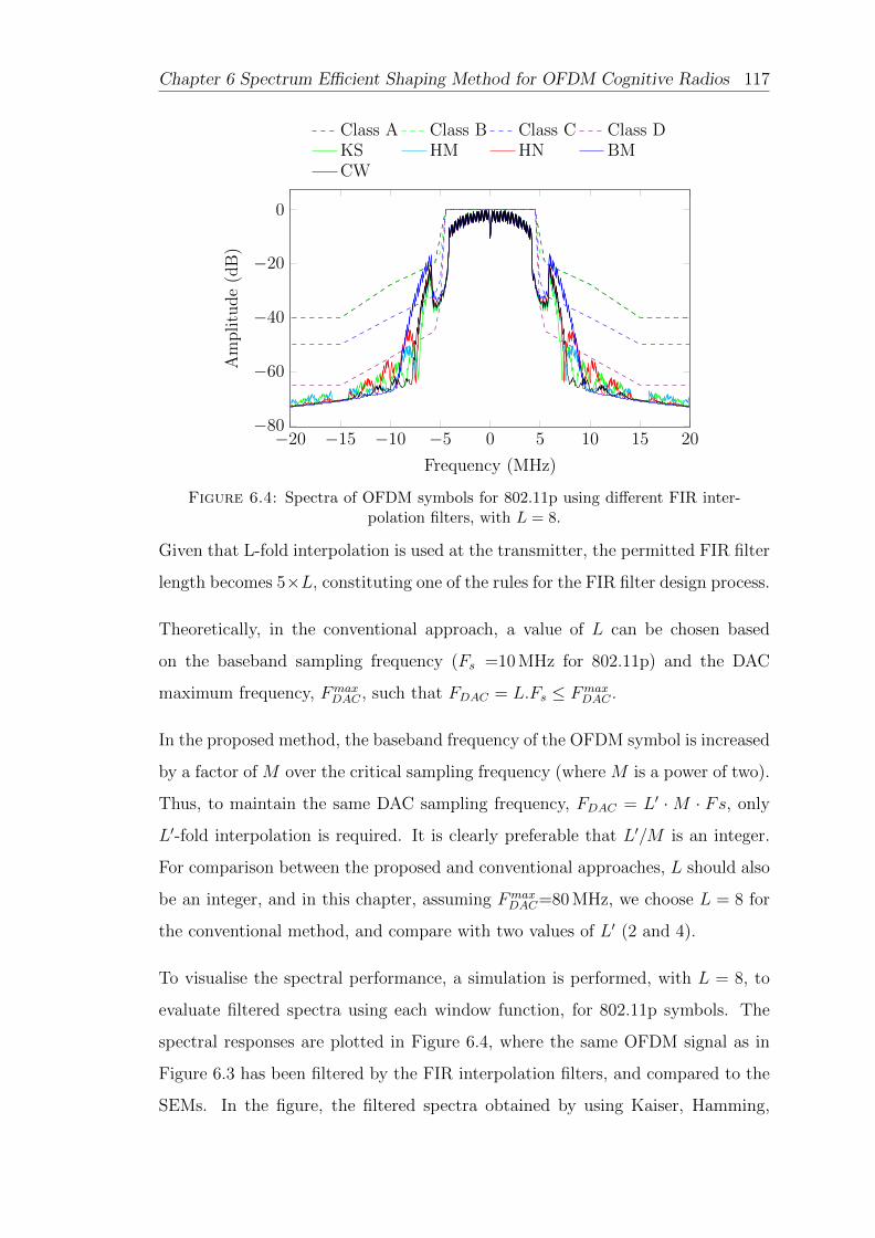
Chapter 6 Spectrum Efficient Shaping Method for OFDM Cognitive Radios 117
−20 −15 −10 −5 0 5 10 15 20−80
−60
−40
−20
0
Frequency (MHz)
Am
plitu
de
(dB
)
Class A Class B Class C Class DKS HM HN BMCW
Figure 6.4: Spectra of OFDM symbols for 802.11p using different FIR inter-polation filters, with L = 8.
Given that L-fold interpolation is used at the transmitter, the permitted FIR filter
length becomes 5×L, constituting one of the rules for the FIR filter design process.
Theoretically, in the conventional approach, a value of L can be chosen based
on the baseband sampling frequency (Fs =10 MHz for 802.11p) and the DAC
maximum frequency, FmaxDAC , such that FDAC = L.Fs ≤ Fmax
DAC .
In the proposed method, the baseband frequency of the OFDM symbol is increased
by a factor of M over the critical sampling frequency (where M is a power of two).
Thus, to maintain the same DAC sampling frequency, FDAC = L′ ·M · Fs, only
L′-fold interpolation is required. It is clearly preferable that L′/M is an integer.
For comparison between the proposed and conventional approaches, L should also
be an integer, and in this chapter, assuming FmaxDAC=80 MHz, we choose L = 8 for
the conventional method, and compare with two values of L′ (2 and 4).
To visualise the spectral performance, a simulation is performed, with L = 8, to
evaluate filtered spectra using each window function, for 802.11p symbols. The
spectral responses are plotted in Figure 6.4, where the same OFDM signal as in
Figure 6.3 has been filtered by the FIR interpolation filters, and compared to the
SEMs. In the figure, the filtered spectra obtained by using Kaiser, Hamming,

Chapter 6 Spectrum Efficient Shaping Method for OFDM Cognitive Radios 118
Hanning, Blackman, and Chebyshev windows are compared (denoted using the
abbreviations in Table 6.2). In each case, two prominent auxiliary peaks, visible
beside the main spectrum, are the biggest impediments to satisfying the SEM
criteria. In detail, the Blackman filtered spectrum slightly exceeds the class A
limits, whereas the remaining filters are able to meet the requirements of classes
A and B but not of classes C and D. In fact, none of the filters are even close to
class C and D compliance. Hence, given the effective guard interval of 802.11p,
FIR filtering clearly does not provide a solution.
The simulation results show that the common filtering methods used at inter-
polated baseband are not even close to meeting the strict SEM requirements of
802.11p. Although not shown here, this is of course equally true of the more strin-
gent 802.11af SEM. This result implies that 802.11p and 802.11af implementations
must rely on sharp front end RF and analogue filtering, which typically results in
an increased total system cost and reduced power efficiency.
6.4 Proposed Spectrum Efficient Shaping Method
The discussions above have revealed that the main challenge to conforming with
strict SEMs is the narrow frequency guard which must accommodate a very sharp
filter transition between pass and stop bands, since the stop-band attenuation
is high. In this section, we briefly explain the method before building upon its
foundation to derive a CR architecture for OFDM spectral leakage mitigation
which we will then evaluate for both 802.11p and 802.11af.
6.4.1 New Spectral Leakage Filtering Method
In a conventional approach, pulse shaping is only employed with small roll-off
factors. This is because large roll-off factors involve longer filters, reducing the
effective guard interval. Given the narrow frequency guard of the OFDM spectrum
for the new standards, and the amount left after accounting for the effects of CIR

Chapter 6 Spectrum Efficient Shaping Method for OFDM Cognitive Radios 119
and matching filters, pulse shaping under such constraints is unable to cancel the
image spectrum: in fact, even if the entire guard interval was to be used, this
may be insufficient for the very stringent class D SEM in 802.11p, and the SEM
of 802.11af. Thus our new method takes a different approach. Instead of using a
large proportion of the guard interval for FIR filtering, we allow the pulse shaping
to occupy a significant portion of the guard space, with large roll-off factors. To
obtain the significant spectral leakage reduction necessary, the frequency guard
needs to be increased. It thus involves introducing a frequency guard extension
technique. Then, given a wider frequency guard, pulse shaping with large roll-off
factors can achieve significant side lobe compression of the OFDM signal, and the
required transition band for FIR filtering is extended, which means a shorter FIR
filter is able to attenuate the image spectrum.
The method thus involves three steps:
• The IFFT length is multiplied by a factor M , and the sampling frequency
similarly increased by a factor M , to maintain the same subcarrier spacing.
Given this, the allocation vector is formed to add data symbols at lower sub-
carriers that are the same as those in the original IFFT, while the remaining
subcarriers are zero-padded.
• Next, pulse shaping is applied in the normal way, to meet the given SEM
constraint.
• Finally, L′-fold interpolation is used to allow simple filtering to remove the
image spectrum.
Based on the proposed approach, we build a flexible CR architecture which is
demonstrated to achieve the SEM requirements for both 802.11p (all classes A, B,
C and D) as well as 802.11af in the UHF band.

Chapter 6 Spectrum Efficient Shaping Method for OFDM Cognitive Radios 120
Figure 6.5: The CR-Based architecture for adaptive OFDM spectral leakageshaping.
6.4.2 Novel CR Filtering Architecture
A CR architecture for OFDM implies the agility to handle non-contiguous (NC)
transmission of symbols (NC-OFDM) as well as the ability to adapt to differ-
ent frequency bands, bandwidths and timing synchronisation regimes. For the
purposes of this chapter, a CR architecture is developed which combines trans-
mission of NC-OFDM symbols with switched sampling frequency, supporting both
802.11p and 802.11af. In particular, the architecture adaptively extends the fre-
quency guard as required, and performs both pulse shaping and FIR interpolation
filtering to meet the most strict SEM requirements of both standards. It should
be understood that this CR architecture is designed to demonstrate compliance
with the more difficult standards: it could trivially be de-rated to the much less
stringent 802.11a and 802.11ac parent standards.
The proposed CR-based transmitter architecture structure is presented in Fig-
ure 6.5, as implemented on a Xilinx FPGA for experimental purposes. As can be
seen, the architecture consists of the baseband sub-modules, including Pil Insert
which flexibly inserts data symbols and pilots from the data modulator, DAT Mod,
into an OFDM symbol according to the current allocation vector (Alloc Vec).
Pre Insert inserts the preamble symbol while IFFT+CP Insert is an IP core that

Chapter 6 Spectrum Efficient Shaping Method for OFDM Cognitive Radios 121
with flexibly reconfigurable IFFT length and CP insertion. PulseShaping per-
forms pulse shaping with a smoothing function for which the roll-off factor can
be changed from small, for relaxed spectral shaping, to large, for more stringent
spectral shaping. L-Fold Inter&FIR performs L′-fold interpolation, with L′ being
controllable on a symbol-by-symbol basis. After interpolation, the FIR block is
used to filter out the image spectrum. In addition, for the CR architecture, the
cognitive control sub-module (CR Ctrl) is used to modify sub-module parameters
to match SEM requirements imposed from the higher layers (i.e. it adjusts timing,
bandwidth, frequency band and SEM requirements). The mixed-mode clock man-
ager (MMCM ) is another integrated IP core used to manage the sampling clock
(Fs), which is set according to the filter performance requirements and operating
frequency band.
In addition, the MMCM allows the transmitter to reduce the degree of filtering
(i.e. degree of spectral leakage shaping) when transmission power is reduced: since
transmit power reduction naturally reduces ICI. This is particularly important for
lower power operating modes in which a lower sampling frequency, less filtering
complexity, and reduced transmission amplitude all contribute to power savings.
Compare this with the 802.11p prototype presented in [108], which was adopted
for direct device-to-device communication between smartphones. That innovative
prototype was able to adaptively increase transmission power to extend commu-
nication range. However, the system was based on an 802.11a hardware solution
and baseband, and did not investigate the increased spectral leakage when the
transmitted signal was amplified to increase range (at which point it would not be
likely to meet the 802.11p SEM requirement).
By contrast, the method proposed and implemented in this chapter, is able to
apply a more stringent SEM filter when transmission power is increased such that
ICI exceeds a given threshold. In particular, CR Ctrl is invoked to change the
IFFT length to M times the original IFFT, while Alloc Vec extends the frequency
guard and MMCM increases Fs according to the required IFFT length. Moreover,
CR Ctrl changes PulseShaping to use a large roll-off factor, reduces the L-fold

Chapter 6 Spectrum Efficient Shaping Method for OFDM Cognitive Radios 122
Table 6.3: Hardware Usage for spectral shaping
Method Module IFFT+CPInsert PulseShaping L-FoldInter&FIR
DSPs 18 0 10
FixedArch Slilces 613 36 139
BRAM 1 0 0
DSPs 34 2 12
FlexArch Slilces 1282 41 189
BRAM 1 0 0
interpolation (since L′ ×M is constant) and shortens the FIR length to meet the
more stringent SEMs. On the other hand, when a device and access point are
in closer proximity, the transmission power can be reduced such that the spectral
leakage is small, and thus filtering can be relaxed. In this case, CR Ctrl is invoked
to change the IFFT length back to the original, and employ PulseShaping with a
small roll-off factor. Moreover, L-Fold Inter&FIR switches back to a normal range
in order to reduce the amount of computation.
In order to provide the flexibility for dynamic shaping spectral leakage, the pro-
cessing modules (i.e. IFFT+CPInsert, Pulseshaping, L-FoldInter&FIR) are im-
plemented with the ability to switch operating mode at run time. This in turn
involves an increase in hardware resources compared to a fixed implementation.
Table 6.3 compares the hardware usage of the modules for the proposed flexible
method, FlexArch, and fixed architecture, FixedArch. FlexArch requires a remark-
able further amount of hardware resource compared to the FixedArch. However,
it should be noted that the additional computation needed for signal processing
in the baseband (which uses low cost, low power components), can be more than
compensated for by relaxing the specification of the RF front-end design, since the
analogue filtering requirements are so much less strict.
The following section presents the application of the proposed CR architecture in
performing stringent filtering to achieve the SEM specifications of both 802.11p
and 802.11af, respectively.
Chapter 6 Spectrum Efficient Shaping Method for OFDM Cognitive Radios 123
6.5 Simulation Results and Discussion
6.5.1 Configuration and Performance Evaluation for 802.11p
Based on the signal model and environmental factors discussed in Section 6.2, the
CIR length is assumed to not exceed 60 ns. Therefore, the effective guard interval,
equivalent to the length of 10 samples of the original CP, i.e., 10×100 = 1000 ns, is
used for the pulse shaping and FIR filter. By choosing a DAC sampling frequency
of 80 MHz, the sampling frequency for 802.11p is increased by 8 times (L′.M = 8)
over the original nominal rate of 10 MHz. Based on this configuration, two optional
systems, denoted as Prop1 and Prop2, will now be explored for 802.11p:
Prop1 doubles the size of the IFFT, i.e., M = 2, which means doubling the
sampling frequency to extend the frequency guard, after which 4-fold interpolation,
i.e., L′ = 4, is required to obtain a sampling frequency of 80 MHz.
Prop2 quadruples the size of the IFFT, i.e., M = 4; Then applies 2-fold interpo-
lation, i.e., L′ = 2 to achieve the 80 MHz sampling frequency.
Based on the results in subsection 6.3.1, p2(m) is employed with βNT = 5 ×M .
i.e. equivalent to the length of 5 samples of the original CP, i.e., 500 ns. It should
be noted that, after extending the frequency guard, the number of samples in
the symbol, including CP, is increased M times. Figure 6.6 plots the shaped
spectrum of the proposed method after interpolation in the baseband, at a sample
frequency of 80 MHz. The original spectrum denoted Conv, and the specifications
for classes C and D are also shown. The main spectrum of Prop1 and Prop2
almost satisfy class D. The image spectrum of Prop1 is present at ±20 MHz and
±40 MHz whereas Prop2 has an image spectrum at ±40 MHz only.
A simpler, shorter-length FIR filter is needed to cancel the image spectra, since
they lie much further away in frequency than for the original approach, Conv. The
remaining guard interval for the transmitter filter and matched filter is 500 ns.
Therefore, the maximum impulse response available for the image rejection FIR

Chapter 6 Spectrum Efficient Shaping Method for OFDM Cognitive Radios 124
−40 −30 −20 −10 0 10 20 30 40
−60
−40
−20
0
Frequency (MHz)
Am
plitu
de(
dB
)
Class C Class D Conv Prop1Prop2
Figure 6.6: Spectrum of 802.11p signal of the proposed CR architecture afterinterpolation.
filter is 250 ns, which is equivalent to 2.5×M.L′ samples at the 80 MHz sampling
frequency.
FIR filters are designed for Prop1 and Prop2 respectively, using a Kaiser window.
For Prop1, since the frequency guard is still relatively narrow, an FIR filter with an
impulse length of 20 samples is required to cancel the image spectrum. Figure 6.7
shows the result of spectrum filtering for Prop1, with the original OFDM spectrum
(Conv) and SEMs for classes C and D overlaid. It can be seen that there are still
two small peaks caused by the image spectrum, but these are compressed by the
FIR filter to meet the class D requirement. Some distortion is noticeable in the
main spectrum due to the effects of the FIR filter.
Prop2 has a wider frequency guard compared to Prop1 and thus its FIR filter
only requires a length of 12 samples to cancel the image spectrum. A remaining
effective guard interval of 200 ns is reserved. Figure 6.8 plots the result of this
degree of spectral filtering for Prop2 and with respect to the class C and D SEMs.
Clearly the image spectrum of Prop2 can be cancelled by a short-length FIR filter,
while suffering less distortion (rounding) to the main passband.

Chapter 6 Spectrum Efficient Shaping Method for OFDM Cognitive Radios 125
−40 −30 −20 −10 0 10 20 30 40
−80
−60
−40
−20
0
Frequency (MHz)
Am
plitu
de
(dB
)
Class C Class D Conv Prop1
Figure 6.7: Spectrum of 802.11p signal using option Prop1 with 20th orderFIR filtering.
−40 −30 −20 −10 0 10 20 30 40
−80
−60
−40
−20
0
Frequency (MHz)
Am
plitu
de
(dB
)
Class C Class D Conv Prop2
Figure 6.8: Spectrum of 802.11p signal for Prop2 with 12th order FIR filtering.
Overall, the simulation results demonstrate that the proposed CR architecture can
meet the specification of class D, the most stringent of the four 802.11p SEMs.
Prop2 obtains better performance in terms of distortion and effective guard inter-
val compared to Prop1, but pays the cost of a higher computational requirement
due to the increased IFFT size.

Chapter 6 Spectrum Efficient Shaping Method for OFDM Cognitive Radios 126
6.5.2 Configuration and Performance Evaluation for 802.11af
Based on the discussion in Section 6.2, if the CIR length is assumed to not exceed
1 us, this is equivalent to 6 samples in the 802.11af CP. Therefore, the effective
guard interval, equivalent to a length of 26 samples of the original CP, is available
for use by the pulse shaping and FIR filters.
By choosing a DAC sampling frequency of 48 MHz, the output sampling frequency
of 802.11af is increased by 8 times (L′.M = 8) compared to the original nominal
frequency (6 MHz). Simulation results for shaping the spectral leakage of 802.11af
are presented here. The proposed method is compared to the conventional ap-
proach which make use of state-of-the-art pulse shaping and FIR filtering. In the
conventional approach, pulse shaping uses 2 samples in the CP for a smoothing
function, and the length of the FIR filter for cancelling the image spectrum is
allowed to extend to 96 (26−22× 8) to avoid ISI. Again, the FIR filter is designed
using a Kaiser window, with a cut-off frequency set to attempt to compress the
signal spectrum to meet the FCC mandated SEM.
Our proposed method quadruples the size of the IFFT (i.e. M = 4), to extend
the frequency guard. Pulse shaping is configured to employ p2(m) from Subsec-
tion 6.3.1, with βNT = 20 ×M . That is equivalent to the length of 20 samples
of the original CP. Then 2-fold interpolation (i.e. L′ = 2), is required to obtain
the sampling frequency of 48 MHz. The maximum allowed FIR filter length for
cancelling the image spectrum without inducing ISI is equivalent to 3 samples of
the original CP. Figure 6.9 illustrates the results of shaping the spectral leakage
for 802.11af using this proposed CR architecture.
Because of the limited length, the band transition of the FIR filter is not narrow
enough. This results in the spectrum of the conventional method, Conv, exhibiting
two side lobes, as well as introducing visible distortion in the main spectrum.
Thus, the conventional method is far from able to meet the SEM requirement for
802.11af. One method that might be considered for achieving this is to deactivate
the outer subcarriers (instead, use null-subcarriers). This can extend the frequency

Chapter 6 Spectrum Efficient Shaping Method for OFDM Cognitive Radios 127
−8 −6 −4 −2 0 2 4 6 8−80
−60
−40
−20
0
Frequency (MHz)
Am
plitu
de
(dB
)
802.11af SEM Conv Prop
Figure 6.9: Spectrum of 802.11af signal using the proposed CR architecture.
guard, but clearly results in a loss of spectral efficiency. Reducing transmission
power is also possible, but is similarly unattractive since it would adversely impact
range – in fact the power reduction needed to bring the Conv transmission within
the SEM envelope is not small. For example, the 802.11af prototype hardware in
[104] requires the transmitted power to be attenuated by 20dB to satisfy the SEM
specifications.
On the other hand, the spectrum of the proposed CR architecture, denoted in
Figure 6.9 as Prop, comfortably meets the SEM specification without impacting
either range or spectral efficiency.
6.5.3 802.11af Spectral Efficiency
Another way of investigating performance is to compute spectral efficiency, given a
flexible allocation of subcarriers. In other words to adjust the number of occupied
subcarriers until the transmission profile fits within the 802.11af SEM, and using
the unoccupied subcarrier space for filter roll off. In the conventional method
(Figure 6.9), about 35 dBc additional filtering would be needed to suppress the
image spectrum at the edge of the channel bandwidth (3 MHz), from -20 dBc, to
-55 dBc.

Chapter 6 Spectrum Efficient Shaping Method for OFDM Cognitive Radios 128
With a 96th order FIR filter as mentioned above for Conv, the transition band
needed to achieve such suppression is estimated, based on the Kaiser window for-
mula in Table 6.2, as being 0.83 MHz. This is equivalent to 21 subcarrier spacings
which would need to be trimmed from each side of the 802.11af channel. Thus the
number of occupied subcarriers would need to be reduced from the standard 114
subcarriers to below 100 in order to give Conv a sufficient guard interval for FIR
filtering.
However, the window formula is only an estimate, and hence the system is simu-
lated here to explore further. In this case, the number of subcarriers is reduced
step-wise in pairs, from the edges working inwards, until the SEM is just satis-
fied. Figure 6.10 plots results with 94 and 92 subcarriers occupied (Conv 92s and
Conv 92s), showing that 92 subcarriers meets the SEM requirement whereas 94
subcarriers does not, by a small margin.
Referring back to Figure 6.9, we also see a clear frequency gap between the spec-
trum of the proposed approach and the SEM. This gap could potentially be ex-
ploited to pack in several more occupied subcarriers. We therefore undertake
simulations to explore this phenomenon, and find that the proposed method is
able to pack in up to 124 employed subcarriers while still satisfying the SEM. This
is also illustrated in Figure 6.10 as Prop 124s.
The results demonstrate that the proposed CR architecture can not only meet
the stringent SEM requirement of 802.11af but could also be used to enhance
spectral efficiency beyond that. Compared to the approach of trimming off edge
carriers needed by an equivalent transmission power conventional system in order
to satisfy the SEM, the proposed approach to CR spectrum shaping increases
spectral efficiency by 32%.

Chapter 6 Spectrum Efficient Shaping Method for OFDM Cognitive Radios 129
−8 −6 −4 −2 0 2 4 6 8−80
−60
−40
−20
0
Frequency (MHz)
Am
plitu
de
(dB
)
802.11af SEM Conv 92s Conv 94s Prop 124s
Figure 6.10: Fitting Filtered Spectrum of 802.11af signal to SEMs.
6.6 Summary
In this chapter, shaping the OFDM leakage spectrum has been investigated at
baseband within a CR architecture, in order to meet stringent spectral emission
mask (SEM) requirements. In particular, this research considers two relatively
new standards, 802.11p and 802.11af, which are defined for the physical layer and
largely based upon existing standards. In both cases, the extended physical layers
are scaled to encourage reuse of existing hardware, devices and designs, but the re-
sulting systems are then subject to much more stringent SEMs. The research relies
upon a combination of interpolation, IFFT length adjustment, pulse shaping and
FIR image suppression filtering, to mitigate against spectral leakage into adjacent
channels. Simulations show that the proposed architecture can meet the specifi-
cation of the four 802.11p classes A to D, as well as the stringent FCC-imposed
SEM for 802.11af in the UHF band. The proposed method is also shown able to
improve the achievable spectral efficiency for reuse of Television White Spaces in
the 802.11af standard by 32%, given equivalent transmission power, compared to
conventional approaches which need to drop the outermost subcarriers in order to
meet SEM requirements. In addition, the architecture has the ability to adaptively
change the degree of spectral leakage filtering in response to transmission power.

Chapter 6 Spectrum Efficient Shaping Method for OFDM Cognitive Radios 130
The computation of filtering can be reduced when transmission power is low, but
when transmission power is high, it is able to extend to meet the strict SEM spec-
ification of both 802.11p and 802.11af. Furthermore, the architecture is capable
of adjusting clock rate, bandwidth, and frequency band on a symbol-by-symbol
basis, in order to implement an agile CR solution.

Chapter 7
An Architecture for
Multi-Standard Cognitive Radios
7.1 Introduction
Cognitive radios that support multiple bands, multiple standards and adapt op-
eration according to environmental conditions are becoming more attractive as
the demand for higher bandwidth and more efficient spectrum use increases. Tra-
ditional implementations in custom ASICs cannot support such flexibility, with
standards changing at a faster pace, while software implementations of baseband
communications fail to achieve the performance required. Hence, FPGAs offer an
ideal platform bringing together flexibility, performance, and efficiency. In this
chapter, we show how we can incorporate our contributions in previous chapters
into a flexible architecture for multi-standard cognitive radios (MSCR). We show
that combining partial reconfiguration (PR) with parameterised modules offers
flexibility while minimising reconfiguration time. When the system adapts to a
new condition (i.e., switching the operating standard), a reconfiguration operation
is performed which may pause or suspend data processing for the duration of the
reconfiguration. Received packets of data may therefore be lost. The reconfig-
uration is required to operate fast enough that the input data buffered during
131

Chapter 7 An Architecture for Multi-Standard Cognitive Radios 132
reconfiguration does not overflow the buffer, leading to entire packets of data be-
ing dropped. Even though there are higher-level protocols available to manage the
retransmission of lost or dropped packets, performing these mechanisms is waste-
ful and may significantly increase the cost in terms of computation and power
consumption.
The work presented in this chapter has also been discussed in:
• T. H. Pham, S. A. Fahmy, and I. V. McLoughlin, “Efficient Multi-Standard
Cognitive Radios on FPGAs,” PhD Forum Poster in Proceedings of the Inter-
national Conference on Field Programmable Logic and Applications (FPL),
Munich, Germany, September 2014 [109].
• T. H. Pham, S. A. Fahmy, and I. V. McLoughlin, “Efficient OFDM-based
baseband processing for Multi-Standard Cognitive Radios on FPGAs,” in
preparation for submission to ACM Transactions on Embedded Computing
Systems.
7.2 Related Work
Most practical CRs are built using powerful general purpose processors to achieve
flexibility through software, but they can fail to offer the computational through-
put required for advanced modulation and coding techniques and they often have
high power consumption. GNU Radio [10] has been a widely used platform in
academia. It is a software application that runs on a computer or an embedded
ARM processor platform, e.g. on the Ettus USRP E100. Computational limita-
tions mean that while it has been successful for investigating CR ideas, it is not
feasible for implementing advanced embedded radios using complex algorithms.
Other software based frameworks like Iris [11], have some limited support for FP-
GAs but suffer from poor bandwidth between software and hardware. Moreover,
the compilation time and reconfiguration time of software defined radio systems
can be long making them unsuitable for adapting to fast changing conditions.

Chapter 7 An Architecture for Multi-Standard Cognitive Radios 133
In an application area with fast moving standards and requiring support for multi-
ple standards, custom ASIC implementation is unlikely to be agile or cost effective
enough to cope with fast-changing standards and operating requirements. In or-
der to address this, Delorme et al. [73] presented a heterogeneous reconfigurable
hardware platform for Cognitive Radio. It can adapt its hardware structure to
support standards like GSM, UMTS, and wireless LAN. Most processing compo-
nents run as embedded software on the nodes in a network-on-chip processor, while
the channel coder and the mapping of the RX chain are implemented inside an
FPGA. Partial reconfiguration (PR) is used to switch the channel coder from one
context to an another depending on SNR. A processor manages data movement
between the different processors, the ASIC, and the FPGA. The need for a large
data buffer and inefficient data transfer mechanisms results in increased power
consumption and reduced throughput.
Other platforms do not propose specific methods for managing a radio’s dynamic
behaviour. KUAR [28] is a mature radio platform built around a fully-featured
Pentium PC with a Xilinx Virtex II FPGA. The baseband processing is acceler-
ated on FPGA and limited to NC-OFDM waveforms based on the IEEE 802.16
standard. Projects at Virginia Tech [110] have shown dynamically assembled ra-
dio structures on FPGAs, where the target radio system is defined at a high-level
with datapaths connecting relatively large functional modules. The modules are
wrapped, and each of them consists of a PR module with complied partial bit-
streams stored in dynamic library. Their online assembly method eliminates the
need for run time compilation, thus affording flexibility. A flexible radio controller
can insert and remove compiled modules to adapt to current conditions. However,
by using low-level reconfiguration circumventing the official PR flow, it is unclear
how this approach can be mapped to newer architectures as they appear.

Chapter 7 An Architecture for Multi-Standard Cognitive Radios 134
CR_Regs
Syn
ch
Fre
Co
mp
FF
T
Rem
ove C
P
Fin
eS
TO
_E
st
IFO
_E
st
&C
h_E
stE
qu
Ph
aseT
rack
DatS
ym
Dem
STD
Alloc_Vec
out of scope system
n scope system Parameterized module
Partial Recog. module
PR port
sys_clk
sys_clk
rx_clkclk_ctrl
clk_ctrl
DA
T_ M
od
FIFO
FIFO
Pil
ot_
Insert
IFF
T+
CP
In
sert
Pr_
Insert
Sp
ec.
Sh
ap
ing
CR Engine
OFDM MSCR Mod
Hig
her
layer
Pro
cessin
g
CR
RF
Fro
nt-
en
d
MMCM
TX
RX
Figure 7.1: The structure of a generic MSCR system
7.3 Proposed OFDM Baseband for MSCR
Figure 7.1 illustrates the proposed structure of baseband modulation for our
OFDM-based MSCR. A mix of partially reconfigurable and parameterised mod-
ules make up the baseband implementation. FIFOs are included to help overcome
the reconfiguration latency when PR modules are reconfigured. While a sink mod-
ule is reconfiguring, these FIFOs store samples from the source until the module
is ready to process data. Since these modules are now just a small part of the
system, buffering is significantly reduced over a more general implementation.
7.3.1 System Description
We developed a prototype MSCR baseband that supports transmitting and re-
ceiving non-contiguous OFDM (NC-OFDM) signals. This system can perform
with different OFDM symbol lengths and frame formats specified differently ac-
cording to multiple standards such as IEEE 802.11 [25], IEEE 802.16 [26], and
IEEE 802.22 [27]. The main specifications of these standards are summarised in
Table 7.1.

Chapter 7 An Architecture for Multi-Standard Cognitive Radios 135
Table 7.1: System specifications of three supported OFDM-based standards.
Specifications IEEE 802.11 IEEE 802.16 IEEE 802.22
Frequency band 2.4–2.5 GHz 5–6 GHz 54–862 MHz
Channel Width 10 MHz 10 MHz 8 MHz
Sampling Frequency 10 MHz 11.52 MHz 9.136 Mhz
FFT size (N) 64 256 2048
CP Length 16 32 512
Number of data carriers 48 192 1440
Number of pilots 4 8 240
The CR implementation is divided into a control plane and data plane. The
data plane performs data processing on the sample data stream. It tranceives
data streams to/from the RF front end through two AXI (Advanced eXtensible
Interface) stream interfaces. For transmission, data is sent from higher layers and
modulated by the data plane. Modulated sample streams are then transferred to
the RF front end to convert to analogue signals and subsequently up-converted
before transmission on the RF channel. For the receiver side, the received signals
are down-converted to the baseband followed by analogue to digital conversion to
form a sample stream. The sample stream is demodulated and processed in the
data plane before being transferred to a higher layer.
To support multiple standards, the data plane must provide the flexibility of
switching baseband modules to the parameters specified by different standards.
AXI Stream interfaces are used for inter-module communication in the data plane
as well as for communication with software. With partial reconfiguration, mod-
ules that that swap into the same region must share the same interfaces, so this
is a suitable abstraction. The AXI Stream protocol also reduces the requirement
for buffering, hence optimising resource usage and total power consumption [85].
Each module has one slave interface to receive data from the previous module and
one master interface to send processed data to the subsequent module.
The control plane is a cognitive radio (CR) engine that is required to perform
adaptive based on the requirements of the application, ultimately deciding which
Chapter 7 An Architecture for Multi-Standard Cognitive Radios 136
base standard to use, and which sub-carriers to enable. A bus register interface
between the control and data planes allows them to communicate. The CR engine
also includes the PR controller that is responsible for loading bitstreams stored in
DRAM into the corresponding PR regions through the ICAP (Internal Configu-
ration Access Port) interface [74] when necessary.
The control plane can be implemented in a number of ways. It can be standalone
software running on a processor core. It can also be hardware in a separate part
of the FPGA. Alternatively, for maximum flexibility and programming support, it
can run on top of an operating system on the processor. By ensuring that symbol
data is processed and moved through the data plane independently of the processor
in the control plane, we are able to achieve high throughput. Normally, the data
plane processes data streams based on a specified standard. An allocation vector
determines which sub-carriers to enable, allowing the radio to respond to varying
channel occupancy conditions. When the frequency band of the current operating
mode is mostly occupied by PUs and IUs, the CR engine instructs the baseband
to switch to another standard or frequency band that is currently (or will soon
be) free for transmission. The PR controller inside the CR engine is required to
download the bitstreams of PR modules according to the new standard. In the
meantime, the CR engine configures the system by writing relevant parameters to
registers in CR Regs such as allocation vectors (Alloc vec), symbol modulation
type (MOD), and standard (STD).
The scope of this chapter focuses on the managing the baseband adaptation in a
way that avoids long configuration time. We do not explore the cognitive func-
tions, nor discuss sensing, which can be implemented in a variety of ways. The
system takes advantage of combining PR with parameterised modules to offer flex-
ibility while minimising reconfiguration time. The CR system is designed to be
capable of operating in burst mode in which it transmits packets as soon as data
is available [111]. If a data packet is ready to be sent but reconfiguration is in
progress, it is buffered in a FIFO. It is then flushed out of FIFO for transmission
after reconfiguration is completed. Since the resource requirements for the trans-
mitter are significantly less than the receiver, reconfiguration time is also shorter.

Chapter 7 An Architecture for Multi-Standard Cognitive Radios 137
We discuss the resource utilisation and reconfiguration time of the transmitter in
Section 7.4. Short reconfiguration time means there is no critical disruption of
the processing chain and loss of transmitted packets. Hence, for the transmitter,
we use a single PR region with the whole transmission chain for simplicity and
flexibility.
The receiver subsystem, by contrast, is required to continuously receive and process
data frames. Furthermore, the hardware usage of the receiver subsystem is much
larger than the transmitter, resulting in longer reconfiguration time. One way to
avoid losing data frames, is to use a large FIFO to store received samples from the
RF front end during reconfiguration, but this can be problematic as this results in
significant resource usage. Our aim here is to reduce reconfiguration time in the
receive chain to mitigate the need for such large FIFOs.
We propose making some modules parameterised, while others are reconfigured
using PR. We explore how to optimise this mix in Section 7.3.2. Now smaller
FIFOs can be used and reconfiguration can be applied at a finer granularity to
minimise the impact of reconfiguration on buffer storage requirements. After re-
configuration is complete, it is necessary to flush the FIFOs and “catch up” with
the received samples. This can be done by increasing the processing clock rate
until the FIFOs are no longer full. Increasing operating speed is done by control-
ling the MMCM module to adjust the speed of the input clock of the receiving
modules, rx clk. Because these modules implemented on FPGA fabric are able to
operate at a frequency higher than 2× the operating clock, no additional resources
are consumed in supporting this increase frequency. We benefit instead from the
improvements in FPGA architectures that mean higher frequencies are achievable
than typically required for baseband processing. It is then reduced back to the
sampling rate (sys clk) to reduce power consumption. The MMCM module is also
required to change the processing rate of data plane according to the different
sampling rates specified in different standards, shown in Table 7.1.

Chapter 7 An Architecture for Multi-Standard Cognitive Radios 138
7.3.2 Module Description
In this section, we detail the design of each functional module shown in Figure 7.1,
showing how to build a multi-standard implementation. There is a tradeoff be-
tween the simplicity, flexibility, but long reconfiguration latency of a PR module
and the increased hardware overhead, complexity, but faster configuration of a
parameterised module. The comparison between the hardware usage of parame-
terised modules for multiple standards and that of individual specified standard
modules is evaluated. In cases where the hardware overhead for parameterisation
is a threshold of the maximum area of a stand-alone module, it is judged as bet-
ter parameterised. For those modules that require significant changes (i.e. the
parameterised overhead is greater than this threshold) or are required to support
unspecified parameters for future standards (such as the preamble), PR can be
used on a per-module basis. Separate bitstreams for each implementation are gen-
erated to be mapped to a PR region. Hence, when switching the entire baseband
from one standard to another, only part of the FPGA needs to be reconfigured.
7.3.2.1 FIFO Buffer (FIFO)
There are two FIFOs at the transmitter side and the receiver side to buffer data
sent from the higher layer and the RF front end, respectively. The FIFO buffers
are implemented using Xilinx FIFO IP cores with 2 port AXI stream interface
configuration. In the normal operation of data stream, one data word is written
to the buffer by the higher layer/the RF front end, while another one is read
out from the buffer by the transmitter side/receiver side in each system clock
cycle. Therefore, the FIFOs normally operate in an almost empty state. When
reconfiguration is required to switch the baseband, the transmitter processing and
receiver processing are suspended. The FIFO buffers store incoming data to avoid
losing frames. Because the system performs in burst mode, the transmitter streams
are not continuous, therefore, the transmitter FIFO can flush stored data during
gaps between bursts. The data buffer is not a critical issue for the transmitter
side.

Chapter 7 An Architecture for Multi-Standard Cognitive Radios 139
Figure 7.2: The receiver FIFO module.
The receiver must, however, process continuously to detect incoming frames, and
so, there is no spare time to flush data that has been buffered in the FIFOs dur-
ing reconfiguration. Therefore, the receiver FIFO is configured with independent
clocks as shown in Figure 7.2. In order to flush stored data in the received FIFO
after reconfiguration, the MMCM increases the receiver processing rate (rx clk)
to be higher than the sampling rate of the RF front end to help empty the FIFO
faster. Once the receiver FIFO is almost empty the processing rate is returned
to the sampling rate to minimise power consumption. Since the FIFO IP cores
support independent write and read clocks, this functionality is seamless to the
stream processing.
7.3.2.2 Synchronisation (Synch)
Our CR system communicates in burst mode. Hence, it must detect the presence
of a frame and estimate the frequency offset required, based upon the preamble
of the received frame. The Synch module performs estimation as discussed in
Chapter 4. Figure 7.3 shows a block diagram of its implementation.
The timing metrics are calculated by using auto-correlation on received samples.
Coarse Time detects the new frame and roughly estimates the start of a frame us-
ing blind estimation that provides generality for application to multiple standards.
By parameterising the length of L, the synchronisation module can effectively per-
form for three current supported standards as well as being extensible for future
standards.

Chapter 7 An Architecture for Multi-Standard Cognitive Radios 140
Figure 7.3: Block diagram of Synchronisation module.
This module is implemented as a parameterised version with parameter L whose
values are defined together with the length of FFT (N), shown in Table 7.2. Com-
binations of L, and N allow it to support multiple standards. The parameterised
values consist not only of the required combinations for 802.11, 802.16, and 802.22,
but also support other combinations for future standards.
Table 7.2: Parameterised values according to supported standardsHH
HHHNL
16 32 64 128 256 512
64 802.11
128
256 802.16
512
1024
2048 802.22
7.3.2.3 Frequency Compensation
The FreComp module performs fractional CFO estimation based on the value of
P passed from the previous module Synch, as described in Chapter 4. Fractional

Chapter 7 An Architecture for Multi-Standard Cognitive Radios 141
Figure 7.4: Block diagram of frequency compensation module.
CFO estimation and compensation are mathematically expressed as:
∆f =∠P
2π LN
r[d] = r[d]e−j2π∆f dN (7.1)
where ∆f is estimated fractional CFO, ∠P denotes the angle of P. Figure 7.4
illustrates the process for frequency compensation. A phase rotation sub-module
is used to compensate fractional CFO by rotating the received sample phase by the
correct angle. This is calculated and accumulated based on estimated fractional
CFO.
φ[d] = φ[d− 1] +∠PL
r[d] = r[d]e−jφ[d] (7.2)
According to (7.2), the computation of FreComp depends on the periodic length
of short preamble that is used to calculate P . Assuming that L is normally defined
as a power of two value, the division by L can be effectively computed by a right
shift. Therefore, this module can be effectively implemented to support multiple
standards by parameterising a right shifter according to the value of L.
7.3.2.4 Fine STO Estimation
FineSTO Est estimates the starting sample of each OFDM symbol. The RF front-
end for MSCR need to access a wide range of frequencies, shown in Table 7.1.

Chapter 7 An Architecture for Multi-Standard Cognitive Radios 142
Figure 7.5: Block diagram of fine STO estimation module.
Depending on the standard being used, the CFO may be large, resulting in the
presence of IFO. Therefore, the implementation of FineSTO Est is based on the
algorithm presented in Chapter 5 that is also robust to IFO. The metric for fine
STO estimation is expressed as:
S[d] =L−1∑m=0
|r[d+m+ L]|2|a[m]|2, (7.3)
when |a[m]| denotes the normalised amplitude of the preamble at the transmitter.
Figure 7.5 shows the block diagram of fine STO estimation. The metric is calcu-
lated based on a multiplierless correlation between received samples and transmit-
ted preamble. Peak Detect finds the maximum value of correlation that is employed
to accurately estimate the STO and Fine Time determines the exact first sample
of the next OFDM symbol (long preamble symbol). However, multiplierless cor-
relation is not flexible and the implementation depends on the preamble which is
different for each standard. Therefore, we employ PR module for the FineSTO Est
module to obtain flexibility. Each supported standard is implemented separately
to a bitstream to be reconfigured at runtime by the CR engine when the under-
lying standard is switched. The PR region must be large enough to house the
largest bitstream among the supported standards.
7.3.2.5 Remove Cyclic Prefix
RemoveCP removes the cyclic prefix attached to each OFDM symbol. The perfor-
mance of this module depends on the length of CP LCP specified differently in each
standards. RemoveCP consists of a counter to count from the beginning of each
symbol and remove the CP samples if the counted value is smaller than LCP This
module can be parameterised by adjusting LCP to support multiple standards.

Chapter 7 An Architecture for Multi-Standard Cognitive Radios 143
7.3.2.6 FFT
FFT is based on the Xilinx FFT/IFFT IP core, which supports modification of
the FFT length at runtime to support different standards. When the standard
is changed, the length of the FFT is modified using the relevant input. This
reconfiguration completes within a few clock cycles.
7.3.2.7 IFO Estimation and Channel Equalisation
IFO Est&Ch EstEqu corrects IFO and performs channel equalisation. IFO results
in a cyclic shift in the frequency domain. IFO is determined based on the method
in Chapter 5:
ε = argmaxε
∣∣∣∣∣N−1∑k=0
Y ∗[k − 1]Y [k]X∗[k − ε]X[k − 1− ε]∣∣∣∣∣ (7.4)
where ε denotes the value of IFO, ε, ε are estimated and trial values of ε, re-
spectively, Y (k) and X(k) denote the kth frequency symbol index of the received
subcarriers and the known transmitted preamble, respectively, and the OFDM
symbol size N is equal to the FFT size.
Figure 7.6 illustrates the block diagram of IFO estimation and channel equalisa-
tion. IFO Correction is performed effectively by cyclically shifting OFDM symbol
corresponding to the estimated IFO estimation.
After compensating for IFO, the effects of the channel and residual STO must
be taken into account to compensate the received sub-carriers. Using information
of the second preamble symbol, the effect of the channel can be estimated. The
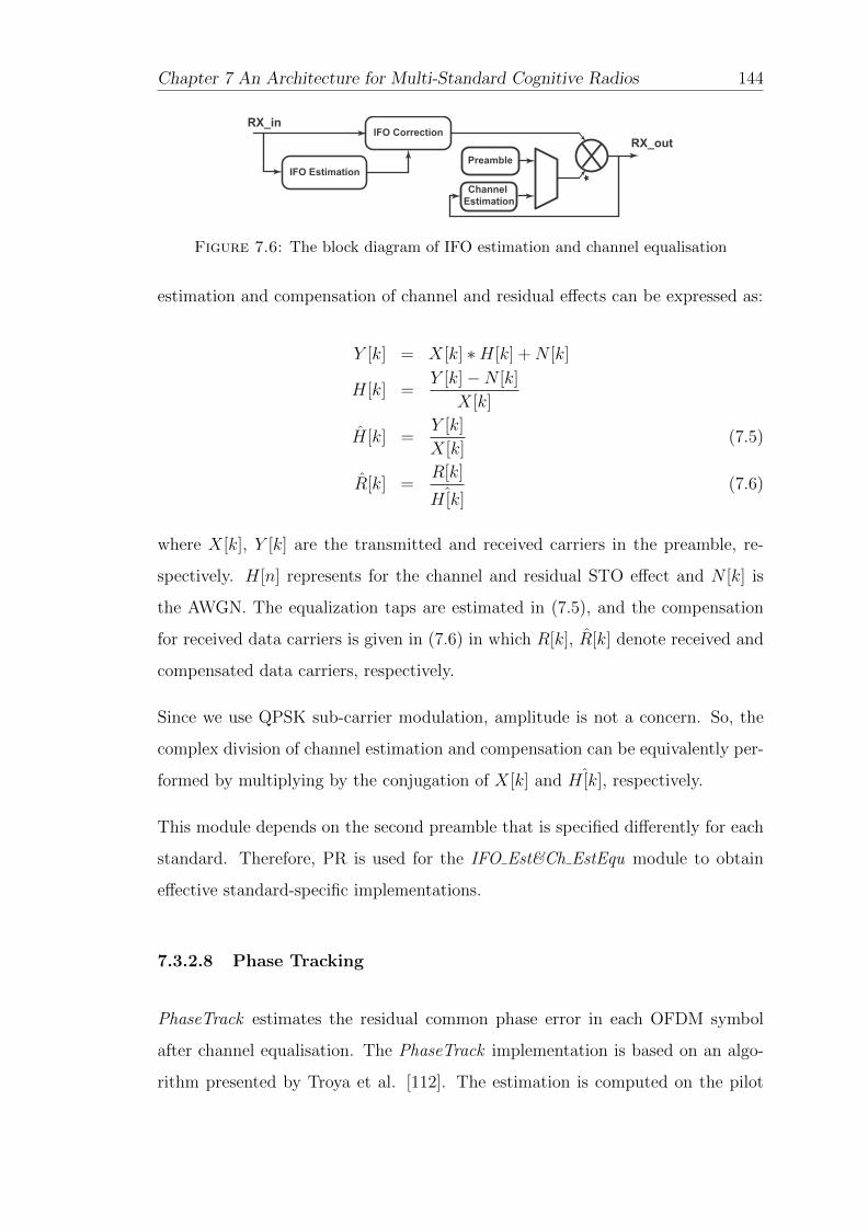
Chapter 7 An Architecture for Multi-Standard Cognitive Radios 144
Figure 7.6: The block diagram of IFO estimation and channel equalisation
estimation and compensation of channel and residual effects can be expressed as:
Y [k] = X[k] ∗H[k] +N [k]
H[k] =Y [k]−N [k]
X[k]
H[k] =Y [k]
X[k](7.5)
R[k] =R[k]
ˆH[k](7.6)
where X[k], Y [k] are the transmitted and received carriers in the preamble, re-
spectively. H[n] represents for the channel and residual STO effect and N [k] is
the AWGN. The equalization taps are estimated in (7.5), and the compensation
for received data carriers is given in (7.6) in which R[k], R[k] denote received and
compensated data carriers, respectively.
Since we use QPSK sub-carrier modulation, amplitude is not a concern. So, the
complex division of channel estimation and compensation can be equivalently per-
formed by multiplying by the conjugation of X[k] and ˆH[k], respectively.
This module depends on the second preamble that is specified differently for each
standard. Therefore, PR is used for the IFO Est&Ch EstEqu module to obtain
effective standard-specific implementations.
7.3.2.8 Phase Tracking
PhaseTrack estimates the residual common phase error in each OFDM symbol
after channel equalisation. The PhaseTrack implementation is based on an algo-
rithm presented by Troya et al. [112]. The estimation is computed on the pilot

Chapter 7 An Architecture for Multi-Standard Cognitive Radios 145
symbols inserted in the OFDM symbol. The transmitted pilots are typically as-
signed the values ±1. The residual phase error causes a phase rotation on received
pilots.
Pk,l = cosθl − α.k.sinθl + j(sinθl − α.k.cosθl), (7.7)
where Pk,l denotes the phase of received pilot which has frequency index k in the
lth OFDM symbol. cosθl + jsinθl is the residual common phase error of the lth
OFDM symbol, and α is the slope of the phase distortion. The residual common
phase error is generally estimated for the supported standards as below:
cosθl =1
NP
∑k∈SP
<{Pk,l}, (7.8)
sinθl =1
NP
∑k∈SP
={Pk,l},
where NP denotes the number of received pilots employed for estimation, SP is
a set of used pilot frequency indices. The Figure 7.7 shows the block diagram
of PhaseTrack. Pilot Extract finds the employed pilots for phase tracking in the
OFDM symbol based on allocation vector (Alloc. Bits). Phase Accumulator com-
putes the residual common phase error according to (7.8). The phase error is
compensated for by multiplying the data carriers by the complex conjugate of the
estimated common phase error. To support multiple standards, NP is parame-
terised and SP can be determined through the allocation vector with the value
shown in Table 7.3
Table 7.3: Allocation vector coding.
Subcarrier Type Allocation Bits
Null 00
Data 10
Positive pilot 01
Negative pilot 11
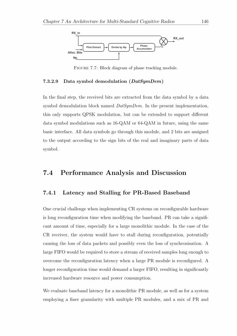
Chapter 7 An Architecture for Multi-Standard Cognitive Radios 146
Figure 7.7: Block diagram of phase tracking module.
7.3.2.9 Data symbol demodulation (DatSymDem)
In the final step, the received bits are extracted from the data symbol by a data
symbol demodulation block named DatSymDem. In the present implementation,
this only supports QPSK modulation, but can be extended to support different
data symbol modulations such as 16-QAM or 64-QAM in future, using the same
basic interface. All data symbols go through this module, and 2 bits are assigned
to the output according to the sign bits of the real and imaginary parts of data
symbol.
7.4 Performance Analysis and Discussion
7.4.1 Latency and Stalling for PR-Based Baseband
One crucial challenge when implementing CR systems on reconfigurable hardware
is long reconfiguration time when modifying the baseband. PR can take a signifi-
cant amount of time, especially for a large monolithic module. In the case of the
CR receiver, the system would have to stall during reconfiguration, potentially
causing the loss of data packets and possibly even the loss of synchronisation. A
large FIFO would be required to store a stream of received samples long enough to
overcome the reconfiguration latency when a large PR module is reconfigured. A
longer reconfiguration time would demand a larger FIFO, resulting in significantly
increased hardware resource and power consumption.
We evaluate baseband latency for a monolithic PR module, as well as for a system
employing a finer granularity with multiple PR modules, and a mix of PR and

Chapter 7 An Architecture for Multi-Standard Cognitive Radios 147
M1 M2 M3 MN
M1 M2 M3 MN
Monolithic PR Module
Reconfiguration
LatencyTc L1 L2 L3 LN
Finer Granularity with Multiple PR Modules
Tc1 Tc2 Tc3 TcN
L1
Ts1
Ts2 Td2
L2Ts3 Td3
TdN
LN
LN-1
Reconfiguration
Latency
Figure 7.8: Comparison of reconfiguration latency for a single and multiplePR modules.
parameterised modules for the case when the system switches to a new baseband.
Figure 7.8 illustrates this latency. We consider a system consisting of N modules.
Tc refers to the reconfiguration time. We assume that a module can not process
data during its reconfiguration time. Li is the computation latency of the ith mod-
ule. Received data can, of course, be processed during the computation latency.
In the case of a large monolithic PR module employed for the system, the system
reconfiguration latency, Lsys, and halting time, Thlt that would require a FIFO to
buffer received data which would otherwise be lost, is calculated as follow:
Lsys = Tc +N∑i=1
(Li)
Thlt = Tc, (7.9)
Finer granularity is possible by dividing the system into multiple sub-modules,

Chapter 7 An Architecture for Multi-Standard Cognitive Radios 148
each of which is implemented in a separate PR region. When a module is com-
pletely configured, it can process the received data while the following module is
configured. Therefore, the system reconfiguration latency and halting time for the
case of multiple PR modules can be calculated as follow;
Lsys =N∑i=1
(Tci) + TdN + LN
Thlt =N∑i=1
(Tsi), (7.10)
where Tdi refers to the processing delay of the following module and Tsi is the
stalling time to wait for configuration of the following module. If the computation
latency of a module, Li, is greater than the reconfiguration time of the following
module, Tci+1, the following module has to delay operation by a duration Tdi before
it receives input data for processing. Otherwise, the previous module is halted a
duration Tsi until the following module is completely configured. The following
module begins processing data just after its configuration is done (Tdi = 0).
Tdi =
Max(Tci, Tdi−1 + Li−1)− Tci i = 2..N,
0 i = 1
(7.11)
Tsi =
Tci −min(Tci, Tdi−1 + Li−1), i = 2..N,
Tc1 i = 1
(7.12)
Substituting the above equations into (7.10),
Lsys =N∑i=1
(Tci) + LN +
(Max(TcN , (Max(...)− TcN−1) + LN−1)− TcN)
Thlt =N∑i=1
(Tci)−N∑i=2
(min(Tci, Tdi−1 + Li−1)), (7.13)

Chapter 7 An Architecture for Multi-Standard Cognitive Radios 149
We can see that system reconfiguration latency and halting time in the case of
multiple PR modules is theoretically reduced thanks to being able to overlap
the reconfiguration and data processing periods. Practically, the reconfiguration
times are usually significantly greater than the processing latencies. This leads to
Tdi = 0 and min(Tci, Tdi−1 +Li−1) = Li−1 resulting in the approximated equations
for (7.13) as below:
Lsys =N∑i=1
(Tci) + LN
Thlt =N∑i=1
(Tci)−N−1∑i=1
(Li), (7.14)
In addition, because of the optimisation in hardware compilation, the overhead of
partitioning into multiple PR modules leads to the fact that∑N
i=1(Tci) is clearly
greater than Tc, in (7.9). Therefore, system reconfiguration latency, Lsys, and
halting time, Thlt in (7.13) may be greater than that in (7.9). Generally, the finer
granularity approach is only efficient in terms of system reconfiguration latency
and halting time if the gain of overlapping the reconfiguration and data processing
is greater than the overhead of partitioning into multiple PR modules.
Through the above analysis and comparison, we propose a new method employing
a mix of PR modules and parameterised modules to obtain a significant reduction
in system reconfiguration latency and halting time. For each module in the pro-
cessing chain, commonalities across different operation modes are analysed. For
modules requiring only minor modifications, parameterised versions are created.
For the ith module to be parameterised, the configuration time of this module
can be eliminated because the parameterised modules can switch operating mode
within one clock period. This approximately results in the following simplified
equations;
Tci ≈ 0
Tsi ≈ 0
Tdi ≈ Tdi−1 + Li−1, (7.15)

Chapter 7 An Architecture for Multi-Standard Cognitive Radios 150
The above equations show the increasing efficiency of overlapping reconfiguration
and data processing leading to a significant reduction in the system reconfiguration
latency and halting time.
7.4.2 Analysing the Proposed OFDM MSCR Approach
We analyse the results of applying this method to the full receiver baseband imple-
mented on a xilinc Virtex 6 FPGA (XC6VLX240T). We compare a large mono-
lithic PR module, finer granularity PR, and the proposed mixture of PR and
parameterisation. Slot based PR is widely used and the only method supported
by Xilinx and Altera tools, and hence we employ it. One if its limitations is that all
resources in the slot are consumed by any component occupying the slot, regardless
of whether it actually uses these components or not. The configuration time for a
component also depends entirely on the slot size, even if it is using only a fraction
of the slot’s resources. There has been some research on alternative methods that
reduce resource wastage by allowing more fine-grained reconfiguration, hence also
reducing reconfiguration time [113]. However, these approaches support a limited
number of FPGA devices, require significant engineering effort and expertise to
port, and remain unsupported in official tool flows. Furthermore, these improve-
ments may still not improve overall reconfiguration latency because it depends on
worst case latency (i.e., the reconfiguration time of the largest components).
To compute the configuration time of a PR module, we generate bitstreams for
all modes. The area of a PR region must satisfy the needs of the largest imple-
mentation it will house. For the monolithic PR module, it is required that the PR
module be able to contain the 802.22 OFDM baseband implementation, which is
the largest receiver implementation among the three target implementations.
Similarly for the fine-grained approach, the configurations of the PR modules are
computed based on the sub-modules of the 802.22 OFDM-based implementation.
Table 7.4 reports the hardware resource usage for each sub-module and transmit-
ter, receiver system for 802.22 on the Virtex 6 device. M1, M2, M3, M4, M5,

Chapter 7 An Architecture for Multi-Standard Cognitive Radios 151
M6, M7, M8 denote the functional modules of the OFDM based system: synchro-
nisation, frequency compensation, fine STO estimation, remove CP, FFT, IFO
estimation and channel equalisation, phase tracking, data symbol demodulation,
respectively. MR, MT are the monolithic receiver and transmitter sub-systems,
respectively.
We then determine the bitsteam size for each functional block according to the
number of occupied CLB, DSP, BRAM columns that provide sufficient required
resources for the block on FPGA floorplan. Figure 7.9 illustrates the bitstream
sizes of each PR module, which we use to calculate configuration time later. The
bitstream sizes of the sub-modules are relatively small compared to the monolithic
PR module for the receiver sub-system. The M3 bitstream is the largest among
the sub-modules. The bitstream of the receiver is nearly triple the size of the
transmitter.
Table 7.4: Resources for 802.22 OFDM-based implementation
modules Slices DSP BRAM
M1(Synch) 498 5 0
M2(FreComp) 474 4 0
M3(FineSTO Est) 2414 0 0
M4(RemoveCP) 23 0 0
M5(FFT ) 1179 15 11
M6(IFO Est&Ch EstEqu) 1249 6 0
M7(Phasetrack) 523 3 0
M8(DatSymDem) 4 0 0
MR(Receiver) 6363 33 11
MT (Transmitter) 1668 15 11
Processing latencies for functional modules are shown for the three standards in
Figure 7.10. We can see that 802.11 has the shortest latency because this standard
uses the shortest FFT length, and hence the shortest symbol length for OFDM
modulation. It should be noted that during this latency the module still receives
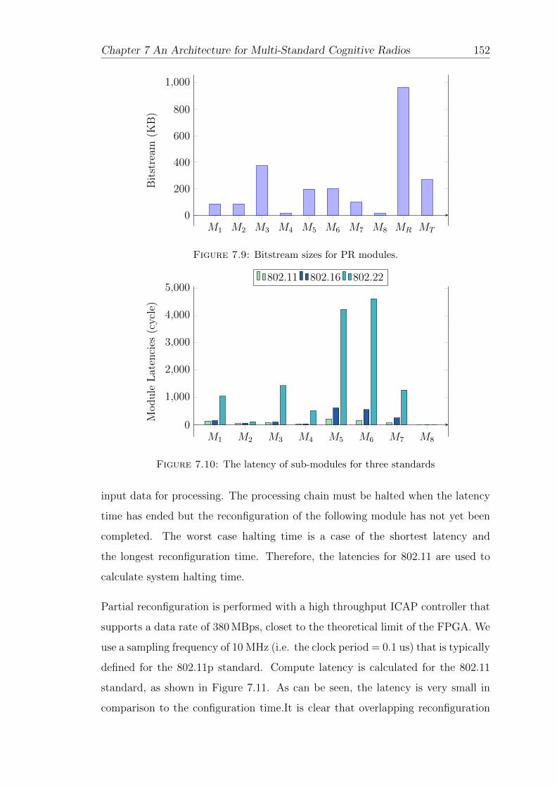
Chapter 7 An Architecture for Multi-Standard Cognitive Radios 152
M1 M2 M3 M4 M5 M6 M7 M8 MR MT
0
200
400
600
800
1,000
Bit
stre
am(K
B)
Figure 7.9: Bitstream sizes for PR modules.
M1 M2 M3 M4 M5 M6 M7 M8
0
1,000
2,000
3,000
4,000
5,000
Module
Lat
enci
es(c
ycl
e)
802.11 802.16 802.22
Figure 7.10: The latency of sub-modules for three standards
input data for processing. The processing chain must be halted when the latency
time has ended but the reconfiguration of the following module has not yet been
completed. The worst case halting time is a case of the shortest latency and
the longest reconfiguration time. Therefore, the latencies for 802.11 are used to
calculate system halting time.
Partial reconfiguration is performed with a high throughput ICAP controller that
supports a data rate of 380 MBps, closet to the theoretical limit of the FPGA. We
use a sampling frequency of 10 MHz (i.e. the clock period = 0.1 us) that is typically
defined for the 802.11p standard. Compute latency is calculated for the 802.11
standard, as shown in Figure 7.11. As can be seen, the latency is very small in
comparison to the configuration time.It is clear that overlapping reconfiguration

Chapter 7 An Architecture for Multi-Standard Cognitive Radios 153
M1 M2 M3 M4 M5 M6 M7 M8
0
200
400
600
800
1,000
Con
figu
rati
onT
ime
(us)
M1 M2 M3 M4 M5 M6 M7 M8
0
5
10
15
Lat
ency
(us)
Configuration Time Latency
Figure 7.11: The configuration time and latency of sub-modules for OFDM-based MSCR system
and data processing is not sufficient to hide reconfiguration delay, and so the
finer granularity approach may not improve significantly over the monolithic PR
module.
The system halting time is an accumulated value of the halting time in each mod-
ule described in (7.12). During the halting time, the processing chain is halted
and a FIFO is required to buffer input samples. Because the halting time of the
synchronisation module depends on the time when a new frame is detected. The
timing offset must be taken into account. Given a scenario of a transmission,
shown in Figure 7.12 when a standard switch is required, Both the transmitter
and receiver spend time to reconfigure the system for the new baseband standard.
In the proposed receiver, the synchronisation module is a parameterised module,
so this module can change its function within a clock period and hence quickly
process input samples. However, a new frame cannot be sent so quickly because
the transmitter is still being reconfigured, resulting in a timing offset in the re-
ceiver. It is thus reasonable that the minimum timing offset can be chosen as the
configuration time of the transmitter whose hardware characteristics were reported
in Table 7.4.
Figure 7.13 shows the system halting time of the three approaches. Mon, Mul,
Pro denote the halting time of the monolithic PR module approach, the multiple

Chapter 7 An Architecture for Multi-Standard Cognitive Radios 154
DA
T_
Mo
d
Pil
ot_
Inse
rt
IFF
T+
CP
In
sert
Pr_
Inse
rt
Sp
ec.
Sh
ap
ing
Sy
nch
Fre
Co
mp
FF
T
Re
mo
ve
CP
Fin
eS
TO
_E
st
IFO
_E
st
&C
h_
Est
Eq
u
Ph
ase
Tra
ck
Da
tSy
mD
em
FIFO
TX RX
Figure 7.12: A scenario of a transmission
0 500 1,000 1,500 2,000 2,500 3,000
Mon
Mul
Pro
Time (us)
Ts1 Ts2 Ts3
Ts4 Ts5 Ts6
Ts7 Ts8 TsR
Figure 7.13: The halting time comparison of the system for three differentapproaches.
PR module approach, and the proposed approach, respectively. Tsn is the halting
time of the corresponding Mn functional module. TsR is the halting time of the
monolithic receiver sub-system.
We can see that the halting time of the multiple PR module approach is greater
than that of the monolithic PR module approach, because the gain achieved by
overlapping reconfiguration and data processing is less than the overhead incurred
by partitioning into multiple PR modules. The proposed approach can signifi-
cantly reduce the halting time to less than one-third of that of the monolithic PR
module approach. This results in a reduction in FIFO buffering requirements.
Figure 7.13 compares the three approaches in terms of system reconfiguration
latency and FIFO buffering requirements. The system latencies are computed
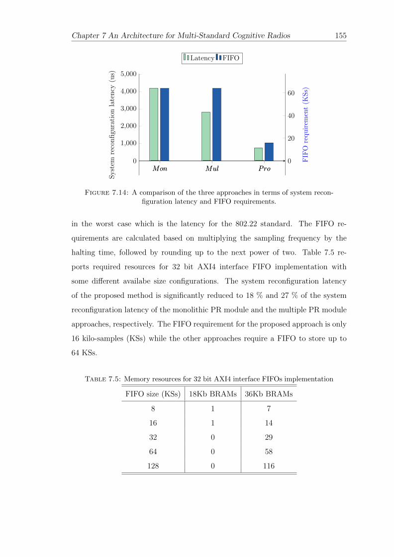
Chapter 7 An Architecture for Multi-Standard Cognitive Radios 155
Mon Mul Pro0
1,000
2,000
3,000
4,000
5,000
Syst
emre
con
figu
rati
onla
ten
cy(u
s)
Mon Mul Pro0
20
40
60
FIF
Ore
qu
irem
ent
(KS
s)
Latency FIFO
Figure 7.14: A comparison of the three approaches in terms of system recon-figuration latency and FIFO requirements.
in the worst case which is the latency for the 802.22 standard. The FIFO re-
quirements are calculated based on multiplying the sampling frequency by the
halting time, followed by rounding up to the next power of two. Table 7.5 re-
ports required resources for 32 bit AXI4 interface FIFO implementation with
some different availabe size configurations. The system reconfiguration latency
of the proposed method is significantly reduced to 18 % and 27 % of the system
reconfiguration latency of the monolithic PR module and the multiple PR module
approaches, respectively. The FIFO requirement for the proposed approach is only
16 kilo-samples (KSs) while the other approaches require a FIFO to store up to
64 KSs.
Table 7.5: Memory resources for 32 bit AXI4 interface FIFOs implementation
FIFO size (KSs) 18Kb BRAMs 36Kb BRAMs
8 1 7
16 1 14
32 0 29
64 0 58
128 0 116

Chapter 7 An Architecture for Multi-Standard Cognitive Radios 156
Figure 7.15: Verification framework.
7.5 System Verification
We now discuss how we verified the correctness and performance of our radio sys-
tem. The overall framework, illustrated in Figure 7.15, evaluates our hardware
design against a MATLAB “golden reference”. The MATLAB prototype serves to
provide the implementation definition as well as providing a source for both ran-
dom and non-random test vectors for each hardware component. Common input
vectors are used to perform OFDM modulation in both implementations. Test-
bench scripts send the input vectors from a database to the implemented system.
Moreover, testbench scripts are also used to monitor the signals generated by the
implementation and store them to a database as output vectors. These output
vectors are then read into MATLAB for comparison against the corresponding
vectors generated by golden reference.
Figure 7.16 shows a block diagram of the baseband system under verification. The
necessary components are connected to a transmitter and a receiver. The output
of the transmitter is buffered and connected to the receiver. It is immediately
obvious that there are many intermediate checkpoints located at the output of
sub-modules that are observed within the implementation and compared to the
simulation for verification.

Chapter 7 An Architecture for Multi-Standard Cognitive Radios 157
Figure 7.16: Block diagram of verified system
The results of some of these verifications are shown in Figure 7.17, Figure 7.18,
and Figure 7.19. These verify the system performing baseband modulation for one
instance of an 802.11 signal. The nomenclature used is emphMM sim and MM rtl
which denote the output of the submodule named MM from the simulation and
implementation respectively. Note from the waveforms plotted, the very close
correspondence of the signal shapes illustrates the underlying correctness of the
implementation.
To consider more closely, Figure 7.17 illustrates verification results from the trans-
mitter. The left figure compares the data symbols and pilots being inserted into
the OFDM symbols (i.e. the module input) while the right figure shows a resulting
OFDM signal (i.e. the module output). This includes the preamble as well as the
OFDM symbols.
Figure 7.18 presents verification results from the receiver in a similar way. The
top-left figure shows the synchronised signal, the top-right figure shows the signal

Chapter 7 An Architecture for Multi-Standard Cognitive Radios 158
Figure 7.17: The verification results of the transmitter.
Figure 7.18: Verification results of the receiver.
with the cyclic prefix stripped. The bottom-left figure plots the demodulated data
symbols after performing FFT. The output of the FFT contains a long pream-
ble that is employed by the subsequent module which performs IFO estimation
and channel equalisation. The output of this module is shown in the bottom-
right. Again, all plots illustrate a close correspondence between simulation and
implementation.
Figure 7.19 presents the observed bit streams at the system input and output.

Chapter 7 An Architecture for Multi-Standard Cognitive Radios 159
Figure 7.19: Verification results of the baseband system.
The left hand figure shows the comparison of output bit streams from simulation
and implementation. Because QPSK is used for data modulation, a data symbol
is modulated with 2 data bits. Therefore, the value is presented from 0 to 3
corresponding to 00, 01, 10, 11 in binary. The right hand figure compares the input
and output bit streams. The data bit stream is modulated at OFDM baseband
and then demodulated. The input and output streams are identical to each other.
Through this careful verification framework, and making use of extensive test-
benches the performance of the system implementation is verified with regard to
the golden reference model in MATLAB. Full implementation on a physical test
platform with over-the-air tests is ongoing work in the research group requiring a
significant engineering effort.
7.6 Summary
We have shown that configuring a radio baseband composed of multiple modules
can be made more efficient in terms of time, and buffering requirements, by mixing
parameterisation and PR. Implement the whole baseband as a single PR module
leads to long reconfiguration time, during which no processing can be performed,
and hence significant FIFO buffering to prevent loss of samples in the receiver.
Breaking the baseband chain into multiple PR modules could be beneficial as it

Chapter 7 An Architecture for Multi-Standard Cognitive Radios 160
would allow individual modules to start processing as they complete their reconfig-
uration, overlapping this processing with the reconfiguration of the next module.
However, since reconfiguration time is significantly higher than the computational
latency, we find that the benefit is outweighed by the overhead of multiple PR
modules. Our proposed approach only applies PR to modules where different
modes are very different in hardware, with other modules designed to be param-
eterisable. As a result, overall halting time is reduced by more than half. The
FIFO buffering requirement of the proposed method is also decreased to 25 % of
that required for the other methods. We are working on finalising a demonstrator
for this approach.

Chapter 8
Conclusions and Future Work
This thesis has presented techniques for implementing robust, low-power cognitive
radios using modern FPGAs. We have shown that the computational performance
of FPGAs allows us to develop techniques for more advanced synchronisation,
leading to robustness in fading channels, that we can control spectral leakage to
satisfy even very strict constraints defined by recent standards, and that a multi-
standard radio can be built to minimise reconfiguration time by mixing the use of
partial reconfiguration and parameterised modules. The contributions made serve
as important building blocks in developing a functional dynamically reconfigurable
OFDM cognitive radio.
This chapter concludes the thesis, highlighting the contributions and suggesting
ideas for future research.
8.1 Summary of Contributions
This thesis has worked towards the implementation of dynamically configurable
cognitive radios on FPGAs. With this goal in mind, we identified key challenges
including robust synchronisation and shaping spectral leakage. We proposed novel
contributions in the field to address these challenges, in each case focusing on
applicability in efficient hardware implementations. We have also explored the
161

Chapter 8 Conclusions and Future Work 162
system-level challenge of reconfiguration time in radios implemented with partial
reconfiguration, and proposed a mixed parametrisation approach for minimising
reconfiguration time.
8.1.1 Robust, Efficient Synchronisation
In Chapter 2, we presented the theory behind OFDM and demonstrated the im-
portance of robust synchronisation, especially in complex channels like those in
moving vehicles, or when building flexible radios with less tuned components. We
proposed a multiplierless correlation method for basic timing synchronisation in
Chapter 3 that can reduce power and area while maintaining performance close to
full cross correlation. We presented a more complex timing metric and its efficient
implementation in Chapter 4, showing robust CFO and STO synchronisation in
frequency selective channels, and a computational complexity close to less robust
standard methods. In Chapter 5 we presented a novel method for CFO estimation
that tolerates larger CFO variations than existing methods, allowing for flexible
radios to be built with support for wide ranging frequency bands without overly ex-
pensive RF components. These methods together offer practical implementations
that are more robust than any other published implementations.
8.1.2 OFDM Spectrum Shaping
We discussed in Chapter 2 that OFDM suffers from large sidelobes due to the
addition of subcarrier sync pulses. In the context of cognitive radios opportunisti-
cally accessing radio spectrum, typically leads to a reduction in usable bandwidth
as some subcarriers are switched off to reduce potential interference with adjacent
channels. In Chapter 6, we presented a novel method incorporating filtering at
the baseband that can offer much better sidelobe suppression, meeting even very
stringent requirements in modern CR standards. We demonstrated this approach
applied to 802.11p and 802.11af waveforms, and demonstrated its feasibility in

Chapter 8 Conclusions and Future Work 163
hardware. We also showed that the proposed architecture could flexibly adjust
this shaping for moving bands in a CR setting.
8.1.3 Multi-Standard Radio Design
In Chapter 7, We presented a detailed analysis of incorporating partial reconfig-
uration for adapting an FPGA-based CR. We showed that while PR offered low
resource utilisation, long reconfiguration time could be a concern. We showed that
mixing PR modules with parametrised modules offered a significant reduction in
reconfiguration time, allowing radios to be implemented with internal buffering to
overcome data loss during reconfiguration. We also showed how a clock frequency
tuning technique could offer seamless recovery following reconfiguration.
8.2 Future Research Directions
Our achievements in this thesis have helped us identify crucial questions to be
explored in future along this line. And while we have been able to test our designs
in hardware, building a fully functional radio system is something that still requires
some engineering design effort.
8.2.1 Increasing Spectrum Efficiency with Shaping for NC-
OFDM
The shaping approach presented in Chapter 6 offers high out of band attenuation,
avoiding interference with neighbouring channels, while allowing use of subcarriers
close to adjacent channels. It could also be applied to in-band shaping in the
context of non-contiguous OFDM signals, where some intermediate subcarriers
are switched off due to the presence of other uses in intermediate bands. This
could result in significant efficiency improvements in the case of highly fragmented
bands, since narrow spaces can still be used effectively

Chapter 8 Conclusions and Future Work 164
8.2.2 Efficiently Adaptive Shaping Spectral Leakage
The static strict SEMs in radio systems can guarantee that the systems mitigate
the effect of ICI. However, the implementation and power cost may be significant.
In practice, adjacent channels are not always occupied and the communication
range can change from time to time. Therefore, statically maintaining a very
strict SEMs may be wasteful in terms of computation. One approach would be
to dynamically modify the SEM based on occupancy of adjacent channels and
current transmit power. This would mean that in some cases the SEM would be
relaxed compared to the static implementation, allowing improved computational
efficiency and lower computational power.
8.2.3 Standardised Software Interface for Multi-Standard
Radio Platform
We have discussed that there are a variety of different cognitive radio platforms,
many of which do include some FPGA capability. However, this interface between
higher layers and hardware baseband processing is often implemented in an ad-hoc
manner. Our group is exploring how a standardised interface might be proposed
to allow higher layer cognitive stacks to be coupled with different baseband sys-
tems, including both the data stream interface, and the control. This must entail
minimal latency, and enable the strengths of the baseband in terms of high data
stream throughput.
8.2.4 Alternative MultiCarrier Modulations Techniques
While OFDM is well established, other multicarrier schemes have been proposed
which offer advantages. Demonstrating efficient mapping of these schemes to high
performance baseband hardware is important for them to gain traction. Gen-
eralised Frequency Division Multiplexing (GFDM) is a new modulation scheme
that overcomes some of OFDM’s limitations. In GFDM, out of band spectrum is

Chapter 8 Conclusions and Future Work 165
compressed by an adjustable pulse shaping filter for individual subcarriers. Trans-
mission efficiency is increased thanks to a two-dimensional data process (grouping
data symbols across subcarriers and time slots). However, it suffers from higher
bit error rates (because of the interference between subcarriers and time slots)
and requires increased computational resources to implement the prototype filter.
A similar structure means a radio supporting both OFDM and GFDM could be
developed, allowing experimentation with this new standard, while offering back-
wards compatibility.
8.2.5 Higher Layer Knowledge to Minimise Reconfigura-
tion Time
As radios support more standards, switching between them can become time-
consuming since many modules need to be reconfigured. One way of overcoming
this is using knowledge about the most likely reconfiguration options to prepare
the require partial bitstreams in advance, or even to drive the design decision
to parameterise some modules that would otherwise use PR. This information
could be forthcoming from higher layers through collaborative decision making or
modelling of the dynamic properties of the channel.
8.3 Summary
This thesis has presented key contributions to allow for the design of dynamically
reconfigurable cognitive radios on FPGAs. FPGAs, especially recent devices like
the Xilinx Zynq, offer an ideal platform for building radios with flexible baseband
processing and high level software control. We are confident that these contribu-
tions will help make this vision a reality in the near future.
Bibliography
[1] B. Farhang-Boroujeny, Signal Processing Techniques for Software Radios.
Lulu Publishing House, 2008.
[2] “Virtex-6 FPGA DSP48E1 Slice: User Guide.” Xilinx, San Jose, CA.
www.xilinx.com/support/documentation/user guides/ug369.pdf, 2011.
[3] T. Schmidl and D. Cox, “Robust frequency and timing synchronization for
OFDM,” IEEE Transactions on Communications, vol. 45, pp. 1613–1621,
Dec. 1997.
[4] C. N. Kishore and V. U. Reddy, “A frame synchronization and frequency
offset estimation algorithm for OFDM system and its analysis,” EURASIP
Journal on Wireless Communications and Networking, vol. 2006, pp. 1–16,
2006.
[5] Federal Communications Commission, “Spectrum policy task force report,”
Tech. Rep. No. 02135, 2002.
[6] R. Rajbanshi, A. M. Wyglinski, and G. J. Minden, “OFDM-based cogni-
tive radios for dynamic spectrum access networks,” in Cognitive Wireless
Communication Networks, pp. 165–188, Springer US, 2007.
[7] M. Cummings and S. Haruyama, “FPGA in the software radio,” IEEE Com-
munications Magazine, vol. 37, pp. 108–112, Feb. 1999.
[8] T. A. Weiss and F. K. Jondral, “Spectrum pooling: An innovative strategy
for the enhancement of spectrum efficiency,” IEEE Radio Communications,
March 2004.
166

BIBLIOGRAPHY 167
[9] R. Rajbanshi, A. M. Wyglinski, and G. J. Minden, “An efficient implemen-
tation of NC-OFDM transceivers for cognitive radios,” in Proceedings of the
1st International Conference on Cognitive Radio Oriented Wireless Networks
and Communications, June 2006.
[10] Free Software Foundation, Inc., “GNU Radio - The GNU Software Radio,”
2009.
[11] P. Sutton, J. Lotze, H. Lahlou, S. Fahmy, K. Nolan, B. Ozgul, T. Rondeau,
J. Noguera, and L. Doyle, “Iris – an architecture for cognitive radio net-
working testbeds,” IEEE Communications Magazine, vol. 48, pp. 114–122,
Sep 2010.
[12] K. Tan, H. Liu, J. Zhang, Y. Zhang, J. Fang, and G. M. Voelker, “Sora: high-
performance software radio using general-purpose multi-core processors,”
Communications of the ACM, vol. 54, no. 1, pp. 99–107, 2011.
[13] T.-H. Kim and I.-C. Park, “Low-power and high-accurate synchronization for
IEEE 802.16d systems,” IEEE Transactions on Very Large Scale Integration
(VLSI) Systems, vol. 16, pp. 1620 –1630, Dec. 2008.
[14] J. Guffey, A. Wyglinski, and G. Minden, “Agile radio implementation of
OFDM physical layer for dynamic spectrum access research,” in Proceedings
of IEEE Global Telecommunications Conference (GLOBECOM), pp. 4051–
4055, Nov. 2007.
[15] A. Recio and P. Athanas, “Physical layer for spectrum-aware reconfigurable
OFDM on an FPGA,” in Proceedings of the Euromicro Conference on Digital
System Design: Architectures, Methods and Tools (DSD), pp. 321–327, Sep.
2010.
[16] T. H. Pham, I. V. McLoughlin, and S. A. Fahmy, “Shaping Spectral Leakage
for IEEE 802.11p Vehicular Communications,” in IEEE Vehicular Technol-
ogy Conference (VTC), May 2014.

BIBLIOGRAPHY 168
[17] J. Mitola and G. Q. M. Jr., “Cognitive radio: making software radios more
personal,” IEEE Personal Communications, vol. 6, pp. 13–18, Aug 1999.
[18] J. Mitola, Cognitive Radio Architecture: The Engineering Foundations of
Radio XML. Wiley, 2006.
[19] A. L. Recio, Spectrum-Aware Orthogonal Frequency Division Multiplexing.
PhD thesis, Virginia Polytechnic Institute and State University, 2010.
[20] A. MacKenzie, J. Reed, P. Athanas, C. Bostian, R. M. Buehrer, L. DaSilva,
S. Ellingson, Y. Hou, M. Hsiao, J.-M. Park, C. Patterson, S. Raman, and
C. da Silva, “Cognitive Radio and Networking Research at Virginia Tech,”
Proceedings of the IEEE, vol. 97, pp. 660–688, April 2009.
[21] C. J. Rieser, T. W. Rondeau, C. Bostian, W. R. Cyre, and T. M. Gal-
lagher, “Cognitive radio engine based on genetic algorithms in a network.”
US Patent 7,289,972, Oct. 2007.
[22] T. W. Rondeau, B. Le, C. J. Rieser, and C. W. Bostian, “Cognitive radios
with genetic algorithms: Intelligent control of software defined radios,” in
Software Defined Radio Forum Technical Conference, pp. C3–C8, 2004.
[23] A. Ghasemi and E. S. Sousa, “Spectrum sensing in cognitive radio net-
works: requirements, challenges and design trade-offs,” IEEE Communica-
tions Magazine, vol. 46, no. 4, pp. 32–39, 2008.
[24] Federal Communications Commission, “Notice of proposed rule making and
order: facilitating oppurtunities for flexible, efficient, and reliable spectrum
use employing cognitive radio technologies,” Tech. Rep. 03-108, 2005.
[25] IEEE std.802.11-2005, IEEE Standard 802 Part11: Wireless LAN Medium
Access Control (MAC) and Physical Layer (PHY) Specifications.
[26] IEEE std.802.16-2009, IEEE Standard for Local and Metropolitan Area Net-
works Part16: Air Interface for Fixed Broadband Wireless Access Systems.
BIBLIOGRAPHY 169
[27] IEEE std.802.22-2011, IEEE Standard for Wireless Regional Area Networks
Part22:Cognitive Wireless RAN Medium Access Control (MAC) and Phys-
ical Layer (PHY) Specifications: Policies and Procedures for Operation in
the TV Bands.
[28] G. J. Minden, J. B. Evans, L. Searl, D. DePardo, V. R. Petty, R. Rajbanshi,
T. Newman, Q. Chen, F. Weidling, J. Guffey, D. Datla, B. Barker, M. Peck,
B. Cordill, A. M. Wyglinsky, and A. Agah, “KUAR: A flexibile software-
defined radio development platform,” in Proceedings of IEEE International
Symposium on New Frontiers in Dynamic Spectrum Access Networks (DyS-
PAN), pp. 17–22, Apr. 2007.
[29] P. Sutton, L. Doyle, and K. Nolan, “A reconfigurable platform for cognitive
networks,” in Proceeding of the International Conference on Cognitive Radio
Oriented Wireless Network Communications (CROWNCOM), 2006.
[30] S. Fahmy, J. Lotze, J. Noguera, L. Doyle, and R. Esser, “Generic software
framework for adaptive applications on FPGAs,” in Proceedings of IEEE
Symposium on Field-Programmable Custom Computing Machines (FCCM),
pp. 55–62, 2009.
[31] J. Lotze, S. A. Fahmy, J. Noguera, B. Ozgul, L. Doyle, and R. Esser, “Devel-
opment framework for implementing FPGA-based cognitive network nodes,”
in IEEE Global Communications Conference (GLOBECOM), 2009.
[32] J. van de Belt, P. D. Sutton, and L. E. Doyle, “Accelerating software radio:
Iris on the Zynq SoC,” in Proceedings of IFIP/IEEE International Confer-
ence on Very Large Scale Integration (VLSI-SoC), pp. 294–295, 2013.
[33] Z. Miljanic, I. Seskar, K. Le, and D. Raychaudhuri, “The WINLAB network
centric cognitive radio hardware platform: WiNC2R,” Mobile Networks and
Applications, vol. 13, no. 5, pp. 533–541, 2008, Springer.

BIBLIOGRAPHY 170
[34] H. So, A. Tkachenko, and R. W. Brodersen, “A unified hardware/soft-
ware runtime environment for FPGA based reconfigurable computers us-
ing BORPH,” ACM Transactions on Embedded Computing Systems, vol. 7,
no. 2, 2008.
[35] K. Amiri, Y. Sun, P. Murphy, C. Hunter, J. R. Cavallaro, and A. Sabharwal,
“WARP, a unified wireless network testbed for education and research,” in
Proceedings of IEEE International Conference on Microelectronic Systems
Education (MSE), pp. 53–54, June 2007.
[36] Free Software Foundation, Inc., “GNU Radio Companion,” 2009.
[37] R. Marlow, C. Dobson, and P. Athanas, “An Enhanced and Embedded GNU
Radio Flow,” in Proceedings of the International Conference on Field Pro-
grammable Logic and Applications (FPL), pp. 1–4, 2014.
[38] A. Love, W. Zha, and P. Athanas, “In pursuit of instant gratification for
FPGA design,” in Proceedings of the International Conference on Field Pro-
grammable Logic and Applications (FPL), pp. 1–8, 2013.
[39] C. Dick and F. Harris, “FPGA implementation of an OFDM PHY,” in
Conference Record of the Thirty-Seventh Asilomar Conference on Signals,
Systems and Computers, vol. 1, pp. 905 – 909, Nov. 2003.
[40] A. Fort, J.-W. Weijers, V. Derudder, W. Eberle, and A. Bourdoux, “A
performance and complexity comparison of auto-correlation and cross-
correlation for OFDM burst synchronization,” in Proceedings of IEEE Inter-
national Conference on Acoustics,Speech,and Signal Processing (ICASSP),
vol. 2, pp. II–341–4, april 2003.
[41] K. Wang, J. Singh, and M. Faulkner, “FPGA implementation of an OFDM-
WLAN synchronizer,” in IEEE International Workshop on Electronic De-
sign, Test and Applications (DELTA), pp. 89 – 94, Jan. 2004.

BIBLIOGRAPHY 171
[42] Z. Huang, B. Li, and M. Liu, “A proposed timing synchronization method
for 802.16e downlink,” in International Symposium on Intelligent Signal Pro-
cessing and Communication Systems (ISPACS), pp. 1–4, Dec. 2010.
[43] E.-S. Shim and Y.-H. You, “OFDM integer frequency offset estimator in
rapidly time-varying channels,” in Proceedings of the Asia-Pacific Confer-
ence on Communications, pp. 1–4, 2006.
[44] M. Morelli and M. Moretti, “Integer frequency offset recovery in OFDM
transmissions over selective channels,” IEEE Transactions on Wireless Com-
munications, vol. 7, pp. 5220–5226, Dec. 2008.
[45] Y.-H. You and K.-W. Kwon, “Multiplication-Free Estimation of Integer Fre-
quency Offset for OFDM-Based DRM Systems,” IEEE Signal Processing
Letters, vol. 17, pp. 851–854, Oct. 2010.
[46] K. Lee, S.-H. Moon, S. Kim, and I. Lee, “Sequence Designs for Robust Con-
sistent Frequency-Offset Estimation in OFDM Systems,” IEEE Transactions
on Vehicular Technology, vol. 62, pp. 1389–1394, March 2013.
[47] M. Morelli, L. Marchetti, and M. Moretti, “Integer frequency offset esti-
mation and preamble identification in WiMAX systems,” in Proceedings of
IEEE International Conference on Communications (ICC), pp. 5610–5615,
June 2014.
[48] A. G. Armada and M. Calvo, “Phase noise and sub-carrier spacing effects
on the performance of an OFDM communication system,” IEEE Communi-
cations Letters, vol. 2, 1998.
[49] “IEEE 802 Standard; Part 11; Amendment 5: Television White Spaces
(TVWS) Operation,” Dec. 2013.
[50] S. Shellhammer, A. Sadek, and W. Zhang, “Technical challenges for cog-
nitive radio in the TV white space spectrum,” in Information Theory and
Applications Workshop, pp. 323–333, Feb 2009.

BIBLIOGRAPHY 172
[51] “IEEE 802 Standard; Part 11; Amendment 6: Wireless Access in Vehicular
Environments,” Jul. 2010.
[52] W. Vandenberghe, I. Moerman, and P. Demeester, “Approximation of the
IEEE 802.11p standard using commercial off-the-shelf IEEE 802.11a hard-
ware,” in Proceedings of the International Conference on ITS Telecommuni-
cations (ITST), pp. 21–26, 2011.
[53] J. Fernandez, K. Borries, L. Cheng, B. Kumar, D. Stancil, and F. Bai, “Per-
formance of the 802.11p Physical Layer in Vehicle-to-Vehicle Environments,”
IEEE Transactions on Vehicular Technology, vol. 61, no. 1, pp. 3–14, 2012.
[54] D. Jiang and L. Delgrossi, “IEEE 802.11p: Towards an international stan-
dard for wireless access in vehicular environments,” in Proceedings of IEEE
Vehicular Technology Conference (VTC), pp. 2036–2040, 2008.
[55] “IEEE Standard for Wireless Access in Vehicular Environments-Multi-
Channel Operations,” Dec. 2010.
[56] X. Wu, S. Subramanian, R. Guha, R. White, J. Li, K. Lu, A. Bucceri, and
T. Zhang, “Vehicular Communications Using DSRC: Challenges, Enhance-
ments, and Evolution,” IEEE Journal on Selected Areas in Communications,
vol. 31, no. 9, pp. 399–408, 2013.
[57] I. Macaluso, B. Ozgul, T. Forde, P. Sutton, and L. Doyle, “Spectrum and
Energy Efficient Block Edge Mask-Compliant Waveforms for Dynamic En-
vironments,” IEEE Journal on Selected Areas in Communications, vol. 32,
pp. 307–321, February 2014.
[58] T. Forde, L. Doyle, and B. Ozgul, “Dynamic Block-Edge Masks (BEMs) for
Dynamic Spectrum Emission Masks (SEMs),” in IEEE Symposium on New
Frontiers in Dynamic Spectrum, pp. 1–10, April 2010.
[59] P. Kryszkiewicz and H. Bogucka, “Dynamic determination of spectrum emis-
sion masks in the varying cognitive radio environment,” in Proceedings of

BIBLIOGRAPHY 173
IEEE International Conference on Communications (ICC), pp. 2733–2737,
June 2013.
[60] C. Masse, “A direct-conversion transmitter for WiMAX and WiBro appli-
cations,” RF Design, vol. 29, no. 1, pp. 42–46, 2006.
[61] Y.-M. Chen and I.-Y. Kuo, “Design of lowpass filter for digital down con-
verter in OFDM receivers,” in Proceedings of the International Confer-
ence on Wireless Networks, Communications and Mobile Computing, vol. 2,
pp. 1094–1099, June 2005.
[62] J. Dowle, S. H. Kuo, K. Mehrotra, and I. V. McLoughlin, “FPGA-based
MIMO and space-time processing platform,” in EURASIP Journal of Ap-
plied Signal Processing, pp. 137–137, Jan. 2006.
[63] M. Faulkner, “The effect of filtering on the performance of OFDM systems,”
IEEE Transactions on Vehicular Technology, vol. 49, pp. 1877–1884, Sep.
2000.
[64] I. Kuon, R. Tessier, and J. Rose, “FPGA architecture: Survey and chal-
lenges,” Foundations and Trends in Electronic Design Automation, vol. 2,
pp. 135–253, Feb. 2008.
[65] P. Coussy and A. Morawiec, eds., High-Level Synthesis: From Algorithm to
Digital Circuit. Springer, 2008 ed., Oct. 2008.
[66] Xilinx Inc., UG470 : 7 Series FPGAs Configuration User Guide, Jan. 2013.
[67] Xilinx Inc., DS190: Zynq-7000 All Programmable SoC Overview, Mar. 2013.
[68] Xilinx Inc., UG585: Zynq-7000 All Programmable SoC Technical Reference
Manual, Mar. 2013.
[69] C. Dobson, K. Rooks, and P. Athanas, “A Power-Efficient FPGA-Based Self-
Adaptive Software Defined Radio,” in International Workshop on Power and
Timing Modeling, Optimization and Simulation (PATMOS), 2014.

BIBLIOGRAPHY 174
[70] P. Sedcole, B. Blodget, T. Becker, J. Anderson, and P. Lysaght, “Modular
dynamic reconfiguration in Virtex FPGAs,” IEE Proceedings - Computers
and Digital Techniques, vol. 153, pp. 157–164, May 2006.
[71] E. McDonald, “Runtime FPGA Partial Reconfiguration,” in Proceedings of
IEEE Aerospace Conference, pp. 1–7, Mar. 2008.
[72] J.-P. Delahaye, J. Palicot, C. Moy, and P. Leray, “Partial reconfiguration
of FPGAs for dynamical reconfiguration of a software radio platform,” in
Proceedings of IST Mobile and Wireless Communications Summit, July 2007.
[73] J. Delorme, J. Martin, A. Nafkha, C. Moy, F. Clermidy, P. Leray, and J. Pal-
icot, “A FPGA partial reconfiguration design approach for cognitive radio
based on NoC architecture,” in Joint International IEEE Northeast Work-
shop on Circuits and Systems and TAISA Conference (NEWCAS-TAISA),
pp. 355–358, June 2008.
[74] K. Vipin and S. Fahmy, “A high speed open source controller for FPGA
Partial Reconfiguration,” in Proceedings of the International Conference on
Field-Programmable Technology (FPT), pp. 61–66, Dec 2012.
[75] K. Vipin and S. A. Fahmy, “Automated partitioning for partial reconfig-
uration design of adaptive systems,” in Proceedings of the Reconfigurable
Architectures Workshop (RAW), May 2013.
[76] A. Raghunathan, N. K. Jha, and S. Dey, High-level power analysis and op-
timization. Boston : Kluwer Academic, 1998.
[77] L. Shang, A. S. Kaviani, and B. Kusuma, “Dynamic power consumption
in Virtex-II FPGA family,” in ACM International Symposium on FPGAs,
pp. 157–164, ACM Press, 2002.
[78] J. Anderson and F. Najm, “Interconnect capacitance estimation for FP-
GAs,” in Proceedings of the Asia and South Pacific Design Automation Con-
ference (ASP-DAC), pp. 713–718, 2004.

BIBLIOGRAPHY 175
[79] J. Anderson and F. Najm, “Power estimation techniques for FPGAs,” IEEE
Transactions on Very Large Scale Integration (VLSI) Systems, vol. 12,
no. 10, pp. 1015–1027, 2004.
[80] E. Todorovich, E. Boemo, A. F., and V. J., “Statistical power estimation
for FPGAs,” in Proceedings of the International Conference on Field Pro-
grammable Logic and Applications (FPL), pp. 515–518, 2005.
[81] A. Reimer, A. Schulz, and N. W., “Modelling macromodules for high-level
dynamic power estimation of FPGA-based digital designs,” in Proceed-
ings of the International Symposium on Low Power Electronics and Design
(ISLPED), pp. 151–154, 2006.
[82] K. Danckaert, K. Masselos, F. Cathoor, H. De Man, and C. Goutis, “Strategy
for power-efficient design of parallel systems,” IEEE Transactions on Very
Large Scale Integration (VLSI) Systems, vol. 7, Issue: 2, pp. 258 – 265, Jun
1999.
[83] L. Varga, G. Hosszu, and F. Kovacs, “A low-power design technique for
digital signal processing applications,” in Proceedings of the Mediterranean
Electrotechnical Conference (MEleCon), vol. II, pp. 827–830, 2000.
[84] P. P. Czapski and A. Sluzek, “Power optimization techniques in FPGA de-
vices: A combination of system and low levels,” International Journal of
Electrical, Computer and Systems Engineering, vol. 1, no. 3, pp. 148 –154,
2007.
[85] Q. Liu, G. Constantinides, K. Masselos, and P. Cheung, “Data-reuse ex-
ploration under an on-chip memory constraint for low-power FPGA-based
systems,” IET Computers & Digital Techniques, vol. 3, no. 3, pp. 235–246,
2009.
[86] S. Ahuja, High Level Power Estimation and Reduction Techniques for Power
Aware Hardware Design. PhD thesis, Virginia Polytechnic Institute and
State University, 2010.

BIBLIOGRAPHY 176
[87] C. Deng, “Power analysis for CMOS/BiCMOS circuits,” in International
Symposium on Low Power Electronics and Design, 1994.
[88] P. Landman and J. Rabaey, “Activity-sensitive architectural power analy-
sis,” IEEE Transactions on Computer-Aided Design of Integrated Circuits
and Systems, vol. 15, no. 6, pp. 571–587, 1996.
[89] S. Gupta and F. Najm, “Analytical models for RTL power estimation of
combinational and sequential circuits,” IEEE Transactions on Computer-
Aided Design of Integrated Circuits and Systems, vol. 19, pp. 808–814, 2000.
[90] A. Raghunathan, S. Dey, and N. K. Jha, “High-level macro-modeling and
estimation techniques for switching activity and power consumption,” IEEE
Transactions on Very Large Scale Integration (VLSI) Systems, vol. 11, no. 4,
pp. 538–557, 2003.
[91] “Xpower estimator userguide.” Xilinx, San Jose, CA.
http://www.xilinx.com/support/documentation/sw manuals/xilinx13 2/ug440.pdf,
2012.
[92] K.-W. Yip, Y.-C. Wu, and T.-S. Ng, “Design of multiplierless correlators for
timing synchronization in IEEE 802.11a wireless LANs,” IEEE Transactions
on Consumer Electronics, vol. 49, pp. 107 – 114, Feb. 2003.
[93] L. Hanzo and T. Keller, OFDM and MC-CDMA : A Primer. Wiley-IEEE
Press, 2006.
[94] T. H. Pham, I. V. McLoughlin, and S. A. Fahmy, “Robust and Efficient
OFDM Synchronisation for FPGA-Based Radios,” Circuits, Systems, and
Signal Processing, vol. 33, pp. 2475–2493, Aug. 2014, Springer.
[95] L. Schwoerer, “VLSI suitable synchronization algorithms and architecture
for IEEE 802.11a physical layer,” in Proceedings of IEEE International Sym-
posium on Circuits and Systems (ISCAS), vol. 5, pp. V–721, 2002.
BIBLIOGRAPHY 177
[96] F. Manavi and Y. Shayan, “Implementation of OFDM modem for the phys-
ical layer of IEEE 802.11a standard based on Xilinx Virtex-II fpga,” in Pro-
ceedings of IEEE Vehicular Technology Conference (VTC), vol. 3, pp. 1768
– 1772, May 2004.
[97] V. Erceg, K. V. S. Hari, and M. S. Smith, “Channel models for fixed wireless
applications,” Tech. Rep. IEEE 802.16a-03/01, Jul. 2003.
[98] T. H. Pham, S. A. Fahmy, and I. V. McLoughlin, “Low-power correlation
for IEEE 802.16 OFDM synchronisation on FPGA,” IEEE Transactions on
Very Large Scale Integration (VLSI) Systems, vol. 21, pp. 1549–1553, August
2013.
[99] K. Bang, N. Cho, J. Cho, H. Jun, K. Kim, H. Park, and D. Hong, “A
coarse frequency offset estimation in an OFDM system using the concept of
the coherence phase bandwidth,” IEEE Transactions on Communications,
vol. 49, pp. 1320–1324, Aug. 2001.
[100] M. Park, N. Cho, J. Cho, and D. Hong, “Robust integer frequency offset
estimator with ambiguity of symbol timing offset for OFDM systems,” in
Proceedings of IEEE Vehicular Technology Conference (VTC), pp. 2116–
2120, 2002.
[101] Xilinx Inc., UG389: Spartan-6 FPGA DSP48A1 Slice, August 2009.
[102] G. Acosta-Marum and M.-A. Ingram, “Six time and frequency selective em-
pirical channel models for vehicular wireless LANs,” IEEE Vehicular Tech-
nology Magazine, vol. 2, no. 4, pp. 4–11, 2007.
[103] I. Sen and D. Matolak, “Vehicle - Vehicle Channel Models for the 5-GHz
Band,” IEEE Transactions on Intelligent Transportation Systems, vol. 9,
no. 2, pp. 235–245, 2008.
[104] Z. Lan, K. Mizutani, G. Villardi, and H. Harada, “Design and implemen-
tation of a Wi-Fi prototype system in TVWS based on IEEE 802.11af,” in

BIBLIOGRAPHY 178
Proceedings of IEEE Wireless Communications and Networking Conference
(WCNC), pp. 750–755, April 2013.
[105] E. Bala, J. Li, and R. Yang, “Shaping Spectral Leakage: A Novel Low-
Complexity Transceiver Architecture for Cognitive Radio,” IEEE Vehicular
Technology Magazine, vol. 8, no. 3, pp. 38–46, 2013.
[106] D. Castanheira and A. Gameiro, “Novel Windowing Scheme for Cognitive
OFDM Systems,” IEEE Wireless Communications Letters, vol. 2, no. 3,
pp. 251–254, 2013.
[107] R. J. Kapadia, Digital Filters Theory, Application and Design of Modern
Filters. Wiley VCH, 2012.
[108] P. Choi, J. Gao, N. Ramanathan, M. Mao, S. Xu, C.-C. Boon, S. A. Fahmy,
and L.-S. Peh, “A case for leveraging 802.11p for direct phone-to-phone
communications,” in Proceedings of the International Symposium on Low
Power Electronics and Design (ISLPED), pp. 207–212, ACM, 2014.
[109] T. H. Pham, S. A. Fahmy, and I. V. McLoughlin, “Efficient Multi-Standard
Cognitive Radios on FPGAs,” in Proceedings of the International Conference
on Field Programmable Logic and Applications (FPL), 2014.
[110] P. Athanas, J. Bowen, T. Dunham, C. Patterson, J. Rice, M. Shelburne,
J. Surıs, M. Bucciero, and J. Graf, “Wires on Demand: run-time communi-
cation synthesis for reconfigurable computing,” in Proceedings of the Inter-
national Conference on Field Programmable Logic and Applications (FPL),
2007.
[111] B. Ai, Z.-X. Yang, C.-Y. Pan, J.-H. Ge, Y. Wang, and Z. Lu, “On the
synchronization techniques for wireless OFDM systems,” IEEE Transactions
on Broadcasting, vol. 52, pp. 236–244, June 2006.

BIBLIOGRAPHY 179
[112] A. Troya, K. Maharatna, M. Krstic, E. Grass, U. Jagdhold, and R. Kraemer,
“Efficient Inner Receiver Design for OFDM-Based WLAN Systems: Algo-
rithm and Architecture,” IEEE Transactions on Wireless Communications,
vol. 6, pp. 1374–1385, April 2007.
[113] A. Sohanghpurwala, P. Athanas, T. Frangieh, and A. Wood, “OpenPR: An
Open-Source Partial-Reconfiguration Toolkit for Xilinx FPGAs,” in IEEE
International Symposium on Parallel and Distributed Processing Workshops
and Phd Forum (IPDPSW), pp. 228–235, May 2011.