Technical University of Madrid (UPM)oa.upm.es/36489/1/CARLOS_ARIEL_GARRIDO_MENDOZA.pdf · cial. El...
197
Technical University of Madrid (UPM) School of Naval Architecture and Ocean Engineering (ETSIN) Hydrodynamic forces on heave plates for offshore systems oscillating close to the seabed or the free surface Author: Carlos A. Garrido-Mendoza MEng.Aerospace Engineer Director: Antonio Souto-Iglesias Professor. DMFPA, ETSIN, UPM Codirector: Krish Thiagarajan Alston D and Ada Lee Correll Presidential Chair in Energy. Professor. University of Maine This dissertation is submitted for the degree of Doctor of Philosophy Maritime Technology April 2015
Transcript of Technical University of Madrid (UPM)oa.upm.es/36489/1/CARLOS_ARIEL_GARRIDO_MENDOZA.pdf · cial. El...

Technical University of Madrid (UPM)School of Naval Architecture and Ocean Engineering (ETSIN)
Hydrodynamic forces on heave plates for offshoresystems oscillating close to the seabed or the free
surfaceAuthor:Carlos A. Garrido-MendozaMEng. Aerospace Engineer
Director:Antonio Souto-Iglesias
Professor. DMFPA, ETSIN, UPM
Codirector:Krish Thiagarajan
Alston D and Ada Lee CorrellPresidential Chair in Energy.
Professor. University of Maine
This dissertation is submitted for the degree ofDoctor of PhilosophyMaritime Technology
April 2015


I would like to dedicate this thesis to my loving parents...
iii


Declaration
I hereby declare that except where specific reference is made to the work of others, thecontents of this dissertation are original and have not been submitted in whole or in partfor consideration for any other degree or qualification in this, or any other University. Thisdissertation is the result of my own work and includes nothing which is the outcome of workdone in collaboration, except where specifically indicated in the text.
Carlos A. Garrido-MendozaApril 2015
v


Acknowledgements
I would like to acknowledge Prof. Antonio Souto-Iglesias for giving me quality supervisionand his full support throughout the years. I thank him for the concern he has shown formy academic progress at the Technical University of Madrid, and his encouragement of myfuture research development.
I want to thank Mr. Carlos López-Pavón for providing me with the industrial motivation formy thesis, for giving me access to a substantial amount of experimental data, and for brightideas on porosity and flaps topics.
I would also like to thank Prof. Krish Thiagarajan of Mechanical Engineering Departmentat the University of Maine for his valuable advice and helpful discussions.
I want to thank Prof. Andrea Colagrossi and Mr. Benjamin Bouscasse for their help withthe mathematical formulation and their valuable advices.
I thank to Prof. Jesús Gómez-Goñi for helping with the PhD grant.
I would like to thank to Mr. Elkin Botia-Vera for his help during the experimental cam-paigns.
I also thank to Mr. José Luis Cercós for his help in many aspects of computational fluiddynamics.
I thank to CEHIPAR Ocean Basin staff led by Mr. Adolfo Marón, for conducting some ofthe experiments within the framework of the different projects.
I also want to thank Prof. Longbin Tao of the School of Marine Science and Technology atthe Newcastle University for hosting me during a research leave in 2014.
I would like to thank Mr. José Ignacio Cardesa for his ideas regarding grid turbulence thatled us to the idea of the fractal plate.
I thank all the staff members at the CEHINAV group for their help in different topics.
I acknowledge the funds received from UPM PhD grant program and UPM mobility grants.
vii


Abstract
Offshore wind energy is one of the promising resources which can reduce the fossil fuelenergy consumption and cover worldwide energy demands. Offshore wind turbine conceptsare based on either a fixed structure as a jacket or a floating offshore platform like a semisub-mersible, spar or tension leg platform. Floating offshore wind turbines have the potentialto be an important part of the energy production profile in the coming years. In order toaccomplish this wind integration, these wind turbines need to be made more reliable andcost efficient to be competitive with other sources of energy.
Floating offshore artifacts, such oil rings and wind turbines, may experience resonant heavemotions in sea states with long peak periods. These heave resonances may increase thesystem downtime and cause damage on the system components and as well as on risersand mooring systems. The heave resonant response may be reduced by different means:(1) increasing the damping of the system, (2) keeping the natural heave period outside therange of the wave energy, and (3) reducing the heave excitation forces. A typical example toaccomplish this reduction are “Heave Plates”. Heave plates are used in the offshore industrydue to their hydrodynamic characteristics, i.e., increased added mass and damping.
Conventional offshore hydrodynamic analysis considers a structure in waves, and evaluatesthe linear and nonlinear loads using potential theory. Viscous damping, which is expectedto play a crucial role in the resonant response, is an empirical input to the analysis, and isnot explicitly calculated. The present research has been mainly focused on the predictionof viscous damping and added mass of floating offshore wind turbine heave plates. In thecalculations, the hydrodynamic forces have been measured in order to compute how thehydrodynamic coefficients of added mass1 and damping vary with the KC2 number, whichcharacterises the amplitude of heave motion relative to the diameter of the disc. In addition,
1Added mass is the inertia added to a system because an accelerating or decelerating body must move (ordeflect) some volume of surrounding fluid as it moves through.
2Keulegan-Carpenter number (KC) is a dimensionless quantity that characterises the amplitude of heavemotion relative to the diameter of the disc.
ix

the influence on the hydrodynamic coefficients when the heave plate is oscillating close tothe free surface or the seabed has been investigated. In this process, a new model describingthe work done by damping in terms of the flow enstrophy, is described herein. This newapproach is able to provide a direct correlation between the local vortex shedding processesand the global damping force. The analysis also includes the study of different edges geom-etry, and examines the sensitivity of the damping and added mass coefficients to the porosityof the plate.
A novel porous heave plate based on fractal theory has also been proposed, tested exper-imentally and compared with experimental data obtained by other authors for plates withsimilar porosity.
A numerical solver of Navier Stokes equations, based on the finite volume technique hasbeen applied. It uses the open-source libraries of OpenFOAM (Open source Field OperationAnd Manipulation), to solve 2 incompressible, isothermal immiscible fluids using a VOF(volume of fluid) phase-fraction based interface capturing approach, with optional meshmotion and mesh topology changes including adaptive re-meshing. Numerical results havebeen compared with experiments conducted at Technical University of Madrid (CEHINAV)and CEHIPAR model basins in Madrid and with others performed at School of MechanicalEngineering in The University of Western Australia 3 4. A brief summary of main resultsare presented below:
1. At low KC numbers, a systematic increase in added mass and damping, correspond-ing to an increase in the seabed proximity, is observed. Specifically, for the caseswhen the heave plate is oscillating closer to the free surface, the dependence of thehydrodynamic coefficients is strongly influenced by the free surface.
2. As seen in experiments, a critical KC, where the linear trend of the hydrodynamic co-efficients with KC is disrupted and that depends on the seabed or free surface distance,has been found.
3. The physical behavior of the flow around the critical KC has been explained throughan analysis of the flow vorticity field.
3Wadhwa and Thiagarajan (2009). Wadhwa, H. and Thiagarajan, K. P. Experimental Assessment of Hy-drodynamic Coefficients of Disks Oscillating Near a Free Surface. ASME 28th International Conference onOffshore Mechanics and Arctic Engineering, OMAE, 2009.
4Wadhwa et al. (2010). Wadhwa, H. and Krishnamoorthy, B. and Thiagarajan, K. P. Variation of HeaveAdded Mass and Damping Near Seabed. ASME 29th International Conference on Offshore Mechanics andArctic Engineering, OMAE, 2010.
x

4. The porosity of the heave plates reduces the added mass for the studied porosity at allKC numbers, but the porous heave plates are found to increase the damping coefficientwith increasing amplitude of oscillation, achieving a maximum damping coefficientfor the heave plate with 10% porosity in the entire KC range.
5. Another concept taken into account in this work has been the heave plates with flaps.Numerical and experimental results show that using discs with flaps will increaseadded mass when compared to the plain plate but may also significantly reduce damp-ing.
6. A novel heave plate design based on fractal theory has tested experimentally for dif-ferent submergences and compared with experimental data obtained by other authorsfor porous plates. Results show an unclear behavior in the coefficients and should bestudied further.
Future work is necessary in order to address a series of open questions focusing on 3Deffects, optimization of the heave plates shapes, etc.
xi


Resumen
La energía eólica marina es uno de los recursos energéticos con mayor proyección pudiendocontribuir a reducir el consumo de combustibles fósiles y a cubrir la demanda de energía entodo el mundo. El concepto de aerogenerador marino está basado en estructuras fijas comojackets o en plataformas flotantes, ya sea una semisumergible o una TLP. Se espera que laenergía eólica offshore juegue un papel importante en el perfil de producción energética delos próximos años; por tanto, las turbinas eólicas deben hacerse más fiables y rentables paraser competitivas frente a otras fuentes de energía.
Las estructuras flotantes pueden experimentar movimientos resonantes en estados de la marcon largos períodos de oleaje. Estos movimientos disminuyen su operatividad y puedencausar daños en los componentes eléctricos de las turbinas y en las palas, también en losrisers y moorings. La respuesta de la componente vertical del movimiento puede reducirsemediante diferentes actuaciones: (1) aumentando la amortiguación del sistema, (2) man-teniendo el período del movimiento vertical fuera del rango de la energía de la ola, y (3)reduciendo las fuerzas de excitación verticales. Un ejemplo típico para llevar a cabo estareducción son las "Heave Plates". Las heave plates son placas que se utilizan en la industriaoffshore debido a sus características hidrodinámicas, ya que aumentan la masa añadida y laamortiguación del sistema.
En un análisis hidrodinámico convencional, se considera una estructura sometida a un oleajecon determinadas características y se evalúan las cargas lineales usando la teoría poten-cial. El amortiguamiento viscoso, que juega un papel crucial en la respuesta en resonanciadel sistema, es un dato de entrada para el análisis. La tesis se centra principalmente enla predicción del amortiguamiento viscoso y de la masa añadida de las heave plates us-adas en las turbinas eólicas flotantes. En los cálculos, las fuerzas hidrodinámicas se hanobtenido con el fin de estudiar cómo los coeficientes hidrodinámicos de masa añadida5 y
5Término utilizado para expresar la fuerza de inercia que ejerce el fluido sobre un sólido, debida a laaceleración del mismo sólido.
xiii
amortiguamiento varían con el número de KC6, que caracteriza la amplitud del movimientorespecto al diámetro del disco. Por otra parte, se ha investigado la influencia de la distan-cia media de la ‘heave plate’ a la superficie libre o al fondo del mar, sobre los coeficienteshidrodinámicos. En este proceso, un nuevo modelo que describe el trabajo realizado por laamortiguación en función de la enstrofía, es descrito en el presente documento. Este nuevoenfoque es capaz de proporcionar una correlación directa entre el desprendimiento local devorticidad y la fuerza de amortiguación global. El análisis también incluye el estudio delos efectos de la geometría de la heave plate, y examina la sensibilidad de los coeficienteshidrodinámicos al incluir porosidad en ésta.
Un diseño novedoso de una heave plate, basado en la teoría fractal, también fue analizadoexperimentalmente y comparado con datos experimentales obtenidos por otros autores.
Para la resolución de las ecuaciones de Navier Stokes se ha usado un solver basado en elmétodo de volúmenes finitos. El solver usa las librerías de OpenFOAM (Open source FieldOperation And Manipulation), para resolver un problema multifásico e incompresible, us-ando la técnica VOF (volume of fluid) que permite capturar el movimiento de la superficielibre. Los resultados numéricos han sido comparados con resultados experimentales lleva-dos a cabo en el Canal del Ensayos Hidrodinámicos (CEHINAV) de la Universidad Politéc-nica de Madrid y en el Canal de Experiencias Hidrodinámicas (CEHIPAR) en Madrid, aligual que con otros experimentos realizados en la Escuela de Ingeniería Mecánica de la Uni-versidad de Western Australia 7 8. Los principales resultados se presentan a continuación:
1. Para pequeños valores de KC, los coeficientes hidrodinámicos de masa añadida yamortiguamiento incrementan su valor a medida que el disco se aproxima al fondomarino. Para los casos cuando el disco oscila cerca de la superficie libre, la dependen-cia de los coeficientes hidrodinámicos es más fuerte por la influencia del movimientode la superficie libre.
2. Los casos analizados muestran la existencia de un valor crítico de KC, donde la ten-dencia de los coeficientes hidrodinámicos se ve alterada. Dicho valor crítico depende
6Keulegan-Carpenter (KC), número adimensional que caracteriza la amplitud del movimiento en heave,relativo al diámetro del disco.
7Wadhwa and Thiagarajan (2009). Wadhwa, H. and Thiagarajan, K. P. Experimental Assessment of Hy-drodynamic Coefficients of Disks Oscillating Near a Free Surface. ASME 28th International Conference onOffshore Mechanics and Arctic Engineering, OMAE, 2009.
8Wadhwa et al. (2010). Wadhwa, H. and Krishnamoorthy, B. and Thiagarajan, K. P. Variation of HeaveAdded Mass and Damping Near Seabed. ASME 29th International Conference on Offshore Mechanics andArctic Engineering, OMAE, 2010.
xiv
de la distancia al fondo marino o a la superficie libre.
3. El comportamiento físico del flujo, para valores de KC cercanos a su valor crítico hasido estudiado mediante el análisis del campo de vorticidad.
4. Introducir porosidad al disco, reduce la masa añadida para los valores de KC estu-diados, pero se ha encontrado que la porosidad incrementa el valor del coeficientede amortiguamiento cuando se incrementa la amplitud del movimiento, logrando unmáximo de damping para un disco con 10% de porosidad.
5. Los resultados numéricos y experimentales para los discos con faldón, muestran queusar este tipo de geometrías incrementa la masa añadida cuando se compara con eldisco sólido, pero reduce considerablemente el coeficiente de amortiguamiento.
6. Un diseño novedoso de heave plate basado en la teoría fractal ha sido experimental-mente estudiado a diferentes calados y comparado con datos experimentales obtenidospor otro autores. Los resultados muestran un comportamiento incierto de los coefi-cientes y por tanto este diseño debería ser estudiado más a fondo.
xv


Table of contents
Declaration of Authorship v
Acknowledgements vii
Abstract ix
Resumen xiii
Table of contents xvii
Nomenclature xxii
1 Introduction 11.1 Motivation . . . . . . . . . . . . . . . . . . . . . . . . . . . . . . . . . . . 11.2 Renewable energy sector in Spain . . . . . . . . . . . . . . . . . . . . . . 21.3 Overview of offshore wind technology . . . . . . . . . . . . . . . . . . . . 4
1.3.1 Introduction . . . . . . . . . . . . . . . . . . . . . . . . . . . . . . 41.3.2 Offshore wind technology in Spain . . . . . . . . . . . . . . . . . . 61.3.3 Wind turbine size and development . . . . . . . . . . . . . . . . . 81.3.4 Classification of offshore wind turbines . . . . . . . . . . . . . . . 9
1.4 Damping of heave motion . . . . . . . . . . . . . . . . . . . . . . . . . . . 161.5 Heave plates . . . . . . . . . . . . . . . . . . . . . . . . . . . . . . . . . . 19
1.5.1 Experimental work . . . . . . . . . . . . . . . . . . . . . . . . . . 191.5.2 Modelling . . . . . . . . . . . . . . . . . . . . . . . . . . . . . . . 20
2 Objectives 232.1 Objectives of the study . . . . . . . . . . . . . . . . . . . . . . . . . . . . 23
3 Methodology 253.1 Methodology of the study . . . . . . . . . . . . . . . . . . . . . . . . . . . 25
xvii

Table of contents
4 Physical and numerical modelling 274.1 Introduction . . . . . . . . . . . . . . . . . . . . . . . . . . . . . . . . . . 274.2 Review . . . . . . . . . . . . . . . . . . . . . . . . . . . . . . . . . . . . 274.3 Theoretical formulation . . . . . . . . . . . . . . . . . . . . . . . . . . . . 30
4.3.1 Governing equations . . . . . . . . . . . . . . . . . . . . . . . . . 304.3.2 Mechanical energy . . . . . . . . . . . . . . . . . . . . . . . . . . 314.3.3 Dissipation . . . . . . . . . . . . . . . . . . . . . . . . . . . . . . 33
4.4 Physical model . . . . . . . . . . . . . . . . . . . . . . . . . . . . . . . . 354.4.1 Numerical solution . . . . . . . . . . . . . . . . . . . . . . . . . . 354.4.2 Modelling of FOWT . . . . . . . . . . . . . . . . . . . . . . . . . 374.4.3 Hydrodynamic Force . . . . . . . . . . . . . . . . . . . . . . . . . 384.4.4 Numerical tests . . . . . . . . . . . . . . . . . . . . . . . . . . . . 384.4.5 Experimental tests . . . . . . . . . . . . . . . . . . . . . . . . . . 394.4.6 Numerical model of turbulence . . . . . . . . . . . . . . . . . . . 414.4.7 Computational tool . . . . . . . . . . . . . . . . . . . . . . . . . . 424.4.8 Validation of numerical procedure . . . . . . . . . . . . . . . . . . 43
5 Parametric dependence of hydrodynamic coefficients of a heave plate oscillat-ing near a seabed or a free surface 475.1 Heave plate moving near a seabed . . . . . . . . . . . . . . . . . . . . . . 47
5.1.1 Introduction . . . . . . . . . . . . . . . . . . . . . . . . . . . . . . 475.1.2 Case study description . . . . . . . . . . . . . . . . . . . . . . . . 485.1.3 Mesh generation . . . . . . . . . . . . . . . . . . . . . . . . . . . 505.1.4 Convergence analysis . . . . . . . . . . . . . . . . . . . . . . . . . 515.1.5 Results . . . . . . . . . . . . . . . . . . . . . . . . . . . . . . . . 56
5.2 Heave plate oscillating close to a free surface . . . . . . . . . . . . . . . . 735.2.1 Introduction . . . . . . . . . . . . . . . . . . . . . . . . . . . . . . 735.2.2 Case study description . . . . . . . . . . . . . . . . . . . . . . . . 735.2.3 Mesh generation . . . . . . . . . . . . . . . . . . . . . . . . . . . 735.2.4 Results . . . . . . . . . . . . . . . . . . . . . . . . . . . . . . . . 75
5.3 Analogies Seabed - Free surface . . . . . . . . . . . . . . . . . . . . . . . 91
6 Hydrodynamic coefficients of an oscillating semi-submersible column with aheave plate 936.1 General . . . . . . . . . . . . . . . . . . . . . . . . . . . . . . . . . . . . 936.2 Case study description . . . . . . . . . . . . . . . . . . . . . . . . . . . . 93
6.2.1 Experimental investigation . . . . . . . . . . . . . . . . . . . . . . 93
xviii
Table of contents
6.2.2 CFD calculations. . . . . . . . . . . . . . . . . . . . . . . . . . . . 1006.3 Results . . . . . . . . . . . . . . . . . . . . . . . . . . . . . . . . . . . . . 112
6.3.1 General . . . . . . . . . . . . . . . . . . . . . . . . . . . . . . . . 1126.3.2 Solid heave plate: influence of flow parameters KC, β and submer-
gence of the heave plate s/rd . . . . . . . . . . . . . . . . . . . . . 1136.3.3 Sensitivity study of scale effects . . . . . . . . . . . . . . . . . . . 1186.3.4 Influence of the shape of the heave plate: flaps . . . . . . . . . . . 1196.3.5 Influence of the heave plate porosity . . . . . . . . . . . . . . . . . 1256.3.6 Fractal plate . . . . . . . . . . . . . . . . . . . . . . . . . . . . . . 129
7 Conclusions 1357.1 Conclusions . . . . . . . . . . . . . . . . . . . . . . . . . . . . . . . . . . 1357.2 Future work . . . . . . . . . . . . . . . . . . . . . . . . . . . . . . . . . . 137
8 Thesis Publications 1398.1 Refereed papers . . . . . . . . . . . . . . . . . . . . . . . . . . . . . . . . 1398.2 Conference papers . . . . . . . . . . . . . . . . . . . . . . . . . . . . . . 139
References 141
List of appendices 150
A Energy Eqn. with control Volume. 153
B Decomposition of the dissipation term. 157B.1 Enstrophy integral . . . . . . . . . . . . . . . . . . . . . . . . . . . . . . . 159B.2 Free surface dissipation integral . . . . . . . . . . . . . . . . . . . . . . . 161
C Useful Relations. 165
D Pressure-Velocity Coupling Algorithm. 167
E Volume of Fluid Method. 171
F Fractal Plate Characteristics. 173
xix


Nomenclature
Greek Symbols
β Frequency parameter. Eqn. (4.30)
µ Dynamic viscosity of the fluid [Pa · s]
ν Kinematic viscosity of the fluid [m2/s]
ρ Density of the fluid [kg/m3]
ω Motion angular frequency [rad/s]
Acronyms / Abbreviations
A Motion heave amplitude [m]
A33 Heave added mass [kg]
S w Waterplane area
B33 Heave viscous damping [kg/s]
Ca Added mass coefficient
Cb Damping coefficient
Cd Drag coefficient
Dc Column diameter [m]
Dd Disc diameter [m]
DNS Direct Numerical Simulation
DV M Discrete Vortex Methods
xxi

f Motion frequency [Hz]
F f luid/body(t) Time history of the force that the fluid exerts on the body
FOWT Floating Offshore Wind Turbines
FV M Finite Volume Method
h Elevation of the disc from the seabed [m]
k Unitary vector in the z direction, pointing upwards
K33 Hydrostatic restoring coefficient
KC Keulegan-Carpenter number. Eqn. (4.29)
NS Navier-Stokes
PIV Particle Image Velocimetry
Re Reynolds number, Eqn. (4.31)
s Submergence of the disc from the free surface [s]
T Motion period [s]
T33 Heave period for a semi-submersible, Eqn. (4.32) [s]
T LP Tension Leg Platform
VOF Volume of Fluid
z Heave displacement
z Second order time derivative of the motion
z First order time derivative of the motion
xxii

Chapter 1
Introduction
1.1 Motivation
Offshore technology has experienced a remarkable growth since the 1940s, when offshoredrilling platforms were first used in the Gulf of Mexico. At the present time, a wide varietyof offshore structures are being used, even under severe environmental conditions. These arepredominantly related to oil and gas recovery, but they are also used in other applicationssuch as harbor engineering, ocean energy extraction and more recently in floating windturbines.Difficulties in design and construction are considerable, particularly as structures are beinglocated at ever-increasing depths and are subjected to extremely hostile environmental con-ditions. New technologies and structures have to be developed to reduce the economic andecologic risks. For hostile areas the reduction of harsh weather induced downtime and in-creased safety have become economic factors of increasing importance. Expensive and timeconsuming trial and error parameter studies are necessary to end up with a good design.Deep water offshore structures have been considered as the most reliable and cost effectivesystem for offshore oil and gas exploration. However, these structures are susceptible toresonant behaviour in sea states with long swell condition having peak period lying in therange of 23 to 25 seconds and these natural periods are smaller for smaller artifacts such asfloating wind turbines. An efficient way to reduce the amplitude of responses is to shift theheave natural period of the proposed structure outside the range of wave spectrum. Dampingelements have been used in ships and offshore structures as response reduction devices formaintaining the hydrodynamic response within acceptable limits. The use of such elementshas been mainly based on past experience or using empirical based design approach.Due to the continued growth of the world population and to the more than ever energydemand, renewable energy plays an important role in the development of society, resulting
1

Chapter 1. Introduction
in significant energy security, climate change mitigation, and economic benefits. Renewableenergy resources exist over wide geographical areas, in contrast to other energy sources,which are concentrated in a limited number of countries. A well known renewable energysource is the wind and traditional wind generators have been installed inland for many years.Wind turbines have also been successfully installed at relatively shallow water depths. Thishas typically been done by piled cylinders or gravity based foundations. Offshore windturbines are one of the most promising technologies to provide an adequate response to ourcurrent energy demand. Based mainly on technology from the oil and gas industry, thereare currently different support structure concepts in the market, which intend to achievea satisfactory outcome to the changeable operational conditions and to help making windenergy more cost effective.
The vision for large-scale floating offshore wind turbines (FOWT) was introduced by Pro-fessor William E. Heronemus at the University of Massachusetts in 1972 (Heronemus,1972), but it was not until the mid 1990’s, after the commercial wind industry was wellestablished, that the topic was taken up again by the mainstream research community. Cur-rent fixed-bottom technology has seen limited deployment to water depths of nearly 30 m(shallow waters) (Musial et al., 2004), but the continental shelf is narrow in many coun-tries which means that the offshore wind energy sector must focus, in such countries, on thefloating structures foundations.
1.2 Renewable energy sector in Spain
Spanish renewable energy potential is wide, and well above the domestic energy demand.It could even be said that renewable energies are Spain’s main energy asset. Expressed interms of installable electrical power, Spain has the potential for several terawatts (TW) ofsolar energy. Wind power takes second place, with a potential estimated at approximately340 GW. The country’s hydroelectric potential, estimated at approximately 33 GW, is alsovery high, but the greater part of this potential has already been developed. The remainingtechnologies have a potential near 50 GW with the potential for wave and geothermal energybeing approximately 20 GW each (IDAE, 2011).
Renewable energy sector in Spain represented 42.8% of total energy production in 2014(42.2% in 2013). Overall 27.4% of Spain’s electricity was generated from wind and solarin 2014 (REE, 2014). In absolute terms, renewable generation fell by 1.0% regarding theprevious year, mainly due to the 6.1% drop in wind production. Despite this decline, itshould be noted that wind power was the technology that made the largest contributiontowards the total energy production in the Iberian Peninsula electricity system with more
2
Chapter 1. Introduction 1.2 Renewable energy sector in Spain
than 20%, more than nuclear and any other energy resource. This is really a remarkablemilestone, which should be highlighted. However, Spain is experiencing a negative trend inthe fulfilment of the 2020 renewable energy objectives. Recent reports have shown that thebest-case scenario projection is within the range of 12.6 − 17.1%, far from the forecastedgoal of 20%. The projection also represents a clear breach of the objectives in the NationalAction Plan for Renewable Energy (Spanish initials PANER) (PANER, 2010), which givesa goal of 22.7%, and the plan drawn up by the Spanish government through the Plan forRenewable Energies (PER), which forecasts 20.8% over 2011 − 2020 (IDAE, 2011).
In addition, the situation for renewable energy and especially for wind energy has becomeextremely difficult in Spain during the period in which this PhD was carried out, from early2011 till 2015. In early 2011, a feed-in-tariff was in place and substantial R&D effortsfunded by the government and by private companies (IBERDROLA, ACCIONA, ABEN-GOA, etc) were ongoing, such as CENIT project AZIMUT, within which part of the exper-imental activities of this PhD work were funded. However, on July 12, 2013, the SpanishGovernment approved measures to overhaul electricity sector regulations and composed aset of new rules (Real decreto ley 1/2012, 2012). This regulation removed economic in-centives for new production of electricity from cogeneration, renewable energy and waste.It also removed incentives for constructing these facilities, in order to avoid adding newcosts to the electrical system. As a consequence, the Spanish renewable energy market hasfallen down drastically and wind energy industry, in which Spain was one of the worldwideleading countries, with very promising forecast, has now also broken down into extremecrisis (IREC, 2014). The uncertainty of premiums in Spain means that no one will invest inSpain’s renewable energy market, and the share prices of the corporations most affected bythe suppression of feed-in tariff for new installations have been Iberdrola, EDP Renewablesand Acciona. Fortunately Europe is still supporting wind energy and its research with thetendency moving towards offshore.
The road to the Spanish offshore wind energy began in 2007 when the Ministry of Industryand Environment started to work to define areas suitable for the installation of windmills atsea, concluding that Spain with more than 4800 kilometers of coastline, had many opportu-nities in this field. However, the current technology limited to a few locations the placementof offshore wind farms. As the technology has advanced into deeper water, floating wind tur-bine platforms may be the most economical means for deploying offshore wind turbines atsome sites. Technically, the long-term survivability of floating structures has already beensuccessfully demonstrated by the marine and offshore oil industries over many decades.However, the economics that allowed the deployment of thousands of offshore oil rigs haveyet to be demonstrated for floating wind turbine platforms. Due to the 2012 changes in the
3

Chapter 1. Introduction
regulatory framework, the prospects are not good, in any case, for the development, at themoment, of the floating offshore wind turbines in Spain.
1.3 Overview of offshore wind technology
1.3.1 Introduction
According to Intergovernmental Panel on Climate Change (2012) (IPCC) report, 80% of theworld’s energy supply could come from renewable sources by 2050 and wind energy willplay a major role in electricity generation in 2050. In the growing market for wind energyand due to the limited available onshore locations, the development of offshore wind farmsbecomes more and more important. With a rapid development of technology, the offshorewind power projects have become a trend in many countries. Without doubt, offshore windwill lead technology advances in the wind sector in a near future as it seeks to exploitresources further offshore.
More than 35 GW of new wind power capacity was brought online in 2013, but this was asharp decline in comparison to 2012, when global installations were in excess of 45 GW.The new global total at the end of 2013 was 318.105 GW, representing cumulative marketgrowth of more than 12.5 percent (see Fig. 1.1). For the sixth year in a row, Asia was theworld’s largest regional market for wind energy, with capacity additions totaling just over18.2 GW. In terms of annual installations China regained its leadership position, adding16.1 GW of new capacity in 2013, a significant gain over 2012 when it installed 12.96 GWof new capacity (Global Wind Energy Council, 2013).
Since the first offshore wind farm built in Denmark (Vindeby 5 MW in 1991), offshorewind energy development in Europe has experienced three stages: initial research stage in1980 − 1990; an experimental testing stage in 1991 − 2000; and commercialization stagesince 2001. Today, more than 7 GW of offshore wind power has been installed globally,representing about 2% of total installed wind power capacity. Most of them, 90%, residein 74 wind farms spread over 11 European countries, in which the United Kingdom (UK),Belgium and Germany are the top countries in offshore installed capacity (see Table 1.1and Fig. 1.2). 78.8% of substructures are monopiles, 10.4% are gravity based foundations,jackets account for 4.7%, tripods account for 4.1% and tripiles account for 1.9%. Thereare also two full scale grid connected floating turbines, and two down-scaled prototypes(EWEA, 2015). According to the more ambitious projections, a total of 80 GW could beinstalled by 2020 worldwide, with three quarters of this in Europe.
Thus, if the strong expansion of offshore wind farms continues, it is expected that 40 GW
4

Chapter 1. Introduction 1.3 Overview of offshore wind technology
Fig. 1.1 Global cumulative installed wind capacity 2000−2013. Source: REN21, 2014
Table 1.1 The latest largest operational offshore wind farms in the world. Source:
Wind farm Capacity(MW)
Country Number ofturbines
Commissioned
London Array 630 UK 175 2012Greater Gabbard 504 UK 140 2012Anholt 400 Denmark 111 2013BARD Offshore 1 400 Germany 80 2013West Duddon Sands 389 UK 102 2014Walney 367 UK 102 2012Thorntonbank 325 Belgium 54 2013Sheringham Shoal 315 UK 88 2012Thanet 300 UK 100 2010DanTysk 288 Germany 80 2014Meerwind Süd / Ost 288 Germany 80 2014Lincs 270 UK 75 2013Northwind 216 Belgium 72 2014
of offshore wind farms will be integrated into the grid and provide between 148 TWh ofelectricity to Europe by 2020 which can meet 10% of Europe’s electricity demand. This fig-ure could be boosted to 17% in 2030, according to the European Wind Energy Association(EWEA, 2015). Some European countries such as Germany and the UK, with ambitious
5

Chapter 1. Introduction
Fig. 1.2 Global cumulative offshore installed capacity in 2013. Source: GWEC, 2013
offshore wind plans, have already become the world’s leading offshore wind market.
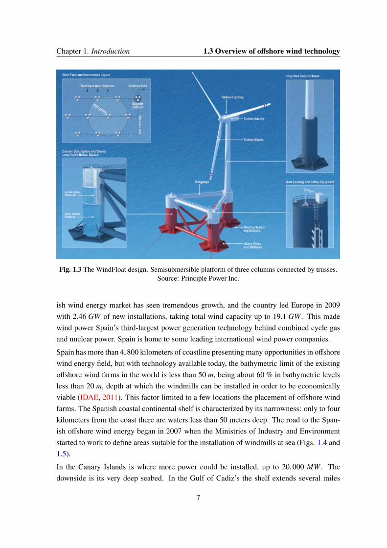
The new projects that were being carried out are for deeper water depths and the cost of thesupport structure and foundation will be proportionally higher than for turbines in shallowwaters. This means that finding an economically feasible design is vital for overall projectviability. Recently, in Portugal a 2 MW prototype offshore wind turbine was installed in thenorth of the country placed on the floating device WindFloat developed by Principle Power(see Fig. 1.3). In the next phase an additional 5 MW turbine will follow. The project isundertaken by EDP Portugal and it expects to achieve a total capacity of 150 MW.
1.3.2 Offshore wind technology in Spain
Spain is endowed with significant wind power resources. According to estimates by the In-stitute for Energy Diversification and Saving (IDAE), published in the National RenewableEnergy Plan for 2011 − 2020 (IDAE, 2011), the technical economical potential for onshorewind power is more than 100 GW by 2020, and more than 150 GW by 2030. The objectiveset for 2020 stands at 35 GW of installed wind capacity. For offshore wind power the currentpotential is estimated at 85 GW with a target of 750 MW by 2020. Up until 2010 the Span-
6
Chapter 1. Introduction 1.3 Overview of offshore wind technology
Fig. 1.3 The WindFloat design. Semisubmersible platform of three columns connected by trusses.Source: Principle Power Inc.
ish wind energy market has seen tremendous growth, and the country led Europe in 2009with 2.46 GW of new installations, taking total wind capacity up to 19.1 GW. This madewind power Spain’s third-largest power generation technology behind combined cycle gasand nuclear power. Spain is home to some leading international wind power companies.
Spain has more than 4,800 kilometers of coastline presenting many opportunities in offshorewind energy field, but with technology available today, the bathymetric limit of the existingoffshore wind farms in the world is less than 50 m, being about 60 % in bathymetric levelsless than 20 m, depth at which the windmills can be installed in order to be economicallyviable (IDAE, 2011). This factor limited to a few locations the placement of offshore windfarms. The Spanish coastal continental shelf is characterized by its narrowness: only to fourkilometers from the coast there are waters less than 50 meters deep. The road to the Span-ish offshore wind energy began in 2007 when the Ministries of Industry and Environmentstarted to work to define areas suitable for the installation of windmills at sea (Figs. 1.4 and1.5).
In the Canary Islands is where more power could be installed, up to 20,000 MW. Thedownside is its very deep seabed. In the Gulf of Cadiz’s the shelf extends several miles
7

Chapter 1. Introduction
Fig. 1.4 Classification of coastal zones for the development of offshore wind projects; Source:Spanish Ministry for Environment, 2009.
from the coast at a depth around 50 meters. Even on the Galician coast, where the waterdepth is greater, the installation of smaller wind farms would be viable.
1.3.3 Wind turbine size and development
Wind turbine sizes have been changing dramatically over the past 40 years. Figure 1.6(Herbert et al., 2007) from the US Department of Energy shows the increase in the size ofthe diameters of installed wind turbines. Figure 1.6 covers both inland and offshore windturbines, and the trend toward large turbines is more pronounced for offshore turbines. Thisis due to the costs associated with constructing and installing the foundations or platformsfor offshore turbines. In the early and mid 1980s, the typical wind turbine size was less than100 kW. By the late 1980s and early 1990s, the turbine sizes had increased from 100 to500 kW. Further, in the mid-1990s, the typical size ranged from 750 to 1000 kW. And bythe late 1990s, the turbine size had gone up to 2.5 MW. Now turbines are available withcapacities above 5 MW.So, nowadays, the research is on a full swing to develop floating wind turbines of highpower. for this reason, in recent years, the studies on the performances of the floating wind
8

Chapter 1. Introduction 1.3 Overview of offshore wind technologyM A P A E Ó L I C O D E E S P A Ñ A
C o m u n i d a d V a l e n c i a n a
A n d a l u c í a
A r a g ó n
C a s t i l l a y L e ó n
G a l i c i a
C a s t i l l a - L a M a n c h a
C a t a l u ñ a
E x t r e m a d u r a
M u r c i a
N a v a r r a
A s t u r i a s
M a d r i d
P a í s V a s c o
L a R i o j a
C a n t a b r i a
I s l a s B a l e a r e s
Jaén
León
Lugo
Ceuta
Ávila
Soria
Cádiz
Cuenca
Teruel
Huesca Girona
Lleida
Murcia
Madrid
Toledo
Huelva
Málaga
Bilbao
Burgos
Zamora
Oviedo
Melilla
Almería
Granada
Córdoba
Sevilla
Segovia
Cáceres
Badajoz
LogroñoOurense
Pamplona
Valencia
Alicante
Albacete
Zaragoza
Palencia
A Coruña
Barcelona
Tarragona
Santander
Salamanca
Valladolid
Pontevedra
Guadalajara
Ciudad Real
Palma de Mallorca
Vitoria - Gasteiz
Castellón de la Plana
Donostia - San Sebastián
Océ
ano
At l
á nt i
c o
M a r M e d i t e r r á n e o
Océ an oAtlán tic o
Ma rMe di terrán eo
0 100 200 300 40050km
Santa Cruz de Tenerife
Las Palmas de Gran Canaria
Vel oc i dad M edi a Anu a l a 80 m d e a l t ura mayo r q ue 6 m/s
m/s
Wind Speed :
< 6
9.5 - 10.0 > 10
6.0 - 6.56.5 - 7.07.0 - 7.57.5 - 8.08.0 - 8.58.5 - 9.09.0 - 9.5
Elaborado por:Julio 2009
Fig. 1.5 Wind map of Spain. Annual average speed at 80 m height; Source: Spanish Ministry forEnvironment, 2009.
turbine for various floater concepts have been carried out by various researchers in order toimprove the energy production capacity of the system.
1.3.4 Classification of offshore wind turbines
1.3.4.1 General
Apart from a few experimental installation, all offshore wind turbines installed to date are onbottom-mounted substructures. Nearly all have been installed in waters shallower than 20 mand these structures are highly dependent on ocean floor conditions. In contrast, much ofthe vast offshore wind resource potential in the USA, China, Japan, Norway and many othercountries, in particular Spain, is available in deeper water. At some water depth, floatingsupport platforms will be the most economical type of support structure.
Recently, some offshore wind power projects are proposed in deeper water, where the windsare of higher velocities. For this reason, wind turbines on floating supports are the bestsolution to utilize the wind resources in those areas. To extend wind turbine systems todeeper water, practical research of offshore floating wind turbine systems is required. Also,
9

Chapter 1. Introduction
Fig. 1.6 Trends of the wind turbine sizes and capacity (US Dept. of Energy).
developing offshore floating wind farms is important because it can minimize the scenerydisturbance, avoid the noise problems generated by wind-driven blades and make use ofextremely abundant deep water wind resources.As afore mentioned wind surrounding the globe has enormous potential to provide alterna-tive source of energy in changing scenarios where global energy demands are increasing.Wind turbines can be placed offshore or onshore but, due to relatively low surface rough-ness of sea surface, offshore locations provide higher wind speed which places offshorewind turbine concept ahead of onshore wind turbine as per the volume of energy productionis concerned. In the process of energy conversion, wind energy from offshore wind turbinecan be converted to electrical power which can be used as power supply. Offshore windturbines are classified into three major types depending upon the water depths such as, Fig.1.7:
1. Shallow water foundation (5-30 meter).
2. Transitional water foundation (30-60 meter).
3. Deep water wind turbine structure (more than 60 meter water depth).
The shallow water wind turbines are generally placed in between 5m−30m water depth andare in general classified as, (Figure 1.8):
10

Chapter 1. Introduction 1.3 Overview of offshore wind technology
Fig. 1.7 Depth ranges for proposed and existing offshore wind turbine foundation designs. Source:NREL.
• Monopile structure.
• Gravity base structure.
• Suction bucket structure.
Fig. 1.8 Three shallow water wind turbine foundations; the monopile, the gravity base, and thesuction bucket from right to left. Source: NREL.
The transitional offshore wind turbine are placed between 30m− 60m water depth and areclassified as, Figure 1.9:
11

Chapter 1. Introduction
• Tripod tower.
• Guyed monopole.
• Full-height jacket.
• Submerged jacket with transition to tube tower.
• Enhanced suction bucked or gravity base.
Fig. 1.9 Transitional Substructure Technology. Source: NREL.
The deep water offshore wind turbines are generally floating structures and are placed inmore than 60m water depth. They are the main focus of our research as heave plates areinstalled in these floating devices to damp heave motions.
1.3.4.2 Floating offshore wind turbines (FOWT)
Floating support structures have appeared in the offshore wind market as a consequence ofthe tendency within this industry to move into deeper waters. Since the first gravity basewas installed, and afterwards monopiles, jackets or tripods, offshore wind parks have gone,step by step, into deeper and deeper waters. The main reason behind this transition lies onthe better quality that wind presents at those locations.Floating wind turbines have the potential to be placed anywhere in the ocean from 60 me-ters upwards to 900 m or beyond. This is a great benefit, because floating platforms allowoffshore wind penetration into places where it may be prohibitive for fixed bottom offshoreturbines. Floating platforms are also much less dependent on seabed conditions than fixed
12
Chapter 1. Introduction 1.3 Overview of offshore wind technology
bottom structures because they do not rely on the ocean floor for support, with mooringline anchors being a notable exception. Many of the floating platform designs are able tobe towed by boats in order to be moved relatively easily. This may reduce costs associ-ated with construction and maintenance. Countries like Japan, Norway or Spain presentthe majority of their offshore wind resource over deep waters. On the other hand, in someEuropean countries, such as the United Kingdom, Germany, Denmark and the Netherlands,where shallow water sites appear to be abundant, the installation of wind parks at thosewater depth levels should still proliferate.Floating offshore wind has been in the works for a while. Consortiums of companies, aca-demic institutions and research organizations have developed different projects of offshorewind floating foundations. However, three main types of floating foundations for offshorewind turbine have been developed so far: Spar foundation, Semi-submersible foundation,and TLP (tension leg platform) foundation (see Fig. 1.10). Roddier et al. (2009) reviewedtypical floating foundations of offshore wind turbines, such as Spars, TLP’s and Semi-submersible/hybrid systems, and the pro-cons of these foundations, design basis and ruleswere listed in detail.In 2008 Blue H Technologies operated the first floating wind turbine using a TLP with an80 kW turbine installed 21 km off the southeast Italy coast in waters 113 metres deep. InSeptember 2009, a 2.3 MW offshore wind turbine which was based on spar structure wasinstalled in Norway to 10 km offshore into 220 metre-deep water (Nielsen et al., 2006) andin late 2012 a semi-submersible type one with 2.0 MW turbine was installed 5 km offshoreof Aguçadoura, north of Porto in Portugal (Roddier et al., 2010).The actual interest of the industry on floating offshore wind turbines is increasing since thelast successful launch and test of real scale prototypes: Hywind in Norway (Hanson et al.,2011), Windfloat in Portugal (Roddier et al., 2010), Mitsui in Japan (Nicholls-Lee et al.,2014) and VolturnUS, the 1 : 8 large scale unit of University of Maine (Marsh, 2014; Viselliet al., 2014). A review on floating offshore wind technology may be found in LLC. (2012),where the status and challenges of this technology are summarized as follows:
• 61% of the US offshore wind resources are in water depths of more than 100 meters;
• Nearly all of Japan’s offshore wind resources are in deep water;
• Various European locations such as off the coast of Norway and in the Mediterraneanrequire floating foundation technology due to water depths;
• UK Round 3 contains some lease areas in water depths which may require floatingtechnology.
13

Chapter 1. Introduction
Fig. 1.10 Floating Offshore Wind Turbine Concepts. Source: Centre for Ships and Ocean StructuresNTNU.
In general terms, the Spar-type has better heave performance than semi-submersibles due totheir deep draft and reduced vertical wave exciting forces, but has larger pitch and roll mo-tions, since the water plane area contribution to stability is reduced. TLPs have small heaveand angular motions, but the complexity and cost of the mooring installation, the changein tendon tension due to tidal variations, and the structural frequency coupling between themast and the mooring system, are three major hurdles for such systems. Semi-submersibleconcepts with a shallow draft and good stability in operational and transit conditions aresignificantly cheaper to tow out, install and commission than spar-buoy, due to their draft.
All these solutions have their origin in the oil & gas industry, but modifications and hybridsare beginning to emerge in their use for wind turbines.
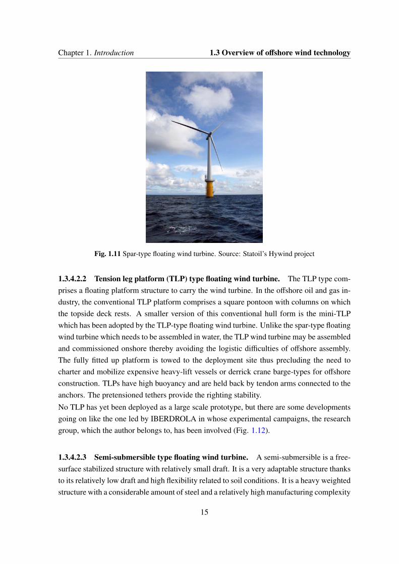
1.3.4.2.1 Spar-type floating wind turbine. The spar buoy is typically a steel or concretecylinder with low water plane area, ballasted with water and/or solid ballast which resultsin a weight-buoyancy stabilized structure with a large draft. The concept uses simple (fewactive components), well-proven technology with inherently stable design and few weak-nesses. Based on the large draft, the spar may however require towing to the deep-water sitein a horizontal position. In such cases the structure needs to be up-ended, stabilized and theturbine is then installed using a crane barge. A spar is generally moored using catenary ortaut spread mooring systems. Statoil’s Hywind is a 2.3 MW prototype that was deployedoutside the west coast of Norway in 2009 was the first floating wind turbine structure in-stalled and is still in operation (see Fig. 1.11).
14
Chapter 1. Introduction 1.3 Overview of offshore wind technology
Fig. 1.11 Spar-type floating wind turbine. Source: Statoil’s Hywind project
1.3.4.2.2 Tension leg platform (TLP) type floating wind turbine. The TLP type com-prises a floating platform structure to carry the wind turbine. In the offshore oil and gas in-dustry, the conventional TLP platform comprises a square pontoon with columns on whichthe topside deck rests. A smaller version of this conventional hull form is the mini-TLPwhich has been adopted by the TLP-type floating wind turbine. Unlike the spar-type floatingwind turbine which needs to be assembled in water, the TLP wind turbine may be assembledand commissioned onshore thereby avoiding the logistic difficulties of offshore assembly.The fully fitted up platform is towed to the deployment site thus precluding the need tocharter and mobilize expensive heavy-lift vessels or derrick crane barge-types for offshoreconstruction. TLPs have high buoyancy and are held back by tendon arms connected to theanchors. The pretensioned tethers provide the righting stability.
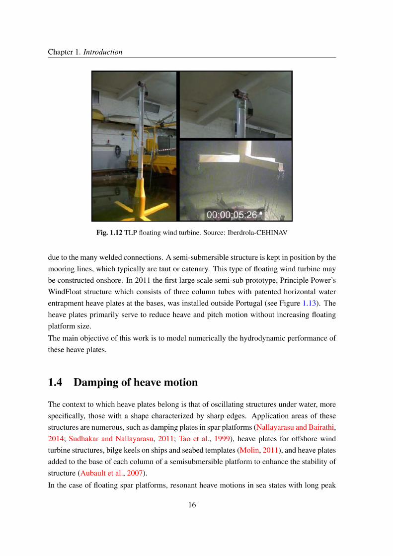
No TLP has yet been deployed as a large scale prototype, but there are some developmentsgoing on like the one led by IBERDROLA in whose experimental campaigns, the researchgroup, which the author belongs to, has been involved (Fig. 1.12).
1.3.4.2.3 Semi-submersible type floating wind turbine. A semi-submersible is a free-surface stabilized structure with relatively small draft. It is a very adaptable structure thanksto its relatively low draft and high flexibility related to soil conditions. It is a heavy weightedstructure with a considerable amount of steel and a relatively high manufacturing complexity
15
Chapter 1. Introduction
Fig. 1.12 TLP floating wind turbine. Source: Iberdrola-CEHINAV
due to the many welded connections. A semi-submersible structure is kept in position by themooring lines, which typically are taut or catenary. This type of floating wind turbine maybe constructed onshore. In 2011 the first large scale semi-sub prototype, Principle Power’sWindFloat structure which consists of three column tubes with patented horizontal waterentrapment heave plates at the bases, was installed outside Portugal (see Figure 1.13). Theheave plates primarily serve to reduce heave and pitch motion without increasing floatingplatform size.
The main objective of this work is to model numerically the hydrodynamic performance ofthese heave plates.
1.4 Damping of heave motion
The context to which heave plates belong is that of oscillating structures under water, morespecifically, those with a shape characterized by sharp edges. Application areas of thesestructures are numerous, such as damping plates in spar platforms (Nallayarasu and Bairathi,2014; Sudhakar and Nallayarasu, 2011; Tao et al., 1999), heave plates for offshore windturbine structures, bilge keels on ships and seabed templates (Molin, 2011), and heave platesadded to the base of each column of a semisubmersible platform to enhance the stability ofstructure (Aubault et al., 2007).
In the case of floating spar platforms, resonant heave motions in sea states with long peak
16

Chapter 1. Introduction 1.4 Damping of heave motion
Fig. 1.13 WindFloat semi-submersible type floating wind turbine. Source: Principle Power Inc.
periods may be experienced. Hydrodynamic damping then becomes a critical factor inkeeping the response amplitude of the structures under acceptable limits. Usually, theseoffshore structures are lightly damped and therefore, although the magnitude of the excitingforce may be small, the response of the system can be large. Haslum and Faltinsen (1999)proposed that the response might be reduced by 3 ways: (1) increasing the damping of thesystem, (2) keeping the natural heave period outside the range of the wave energy, and (3)further reducing the linear heave excitation forces.
Regarding technique number 1, a commonly used device to enhance the damping mecha-nisms in the vertical (heave) direction, is a heave plate, which is usually added at the baseof the structure. This arrangement enhances the vortex shedding process due to isolatedsharp edges, as well as increases the effective vertical mass of the structure, consequentlychanging the hydrodynamic properties of the body in question by introducing extra dampingand increasing its natural period. In Fig. 1.14 the heave plate arrangement for WindFloat(Roddier et al., 2010) semi-submersible design is included (left). In the center, ACCIONAHYPERWIND Project design is included and an image of its column and heave plate ispresented (right). Our research pays significantly attention to ACCIONA design becauseexperimental data is available due to the involvement of the candidate in the experimental
17

Chapter 1. Introduction
and numerical analysis.
Fig. 1.14 Heave plate arrangement for WindFloat (Roddier et al., 2010) semi-submersible design(left). ACCIONA design (center) and one of its columns and heave plate (right).
Relative to technique 2, increasing the mass of the system is expensive and increasing addedmass is also achieved with the use of heave plates. Reducing the water plane area is anotheroption which is usually not viable due to structural reasons.The technique 3, increasing the draft for slender designs reduces waves excitations. Nonethe-less draft is subjected to other considerations like construction, transportation, etc.It is well-known that flow properties get significantly altered in the presence of a close mate-rial boundary or a free surface. However, there are a few researchers that have focused theirworks on the influence on the hydrodynamic characteristics of a structure when movingclose to the seabed or free surface. Lamb (1945, § 137) showed that a sphere constrained tomove in a fluid along a line parallel to a wall experiences an “attraction” towards the wall.Greenhow and Lin (1983) and Faltinsen (1990, §Ch. 9) discussed flow phenomena associ-ated with a cylinder entering and exiting a free surface. The re-alignment of the flow, due toboundary proximity, results in modified pressure and vorticity fields, in turn influencing theforces experienced by the body motion. In some offshore applications such as deploymentof foundation templates and subsea structures, the penetration of a structure through the wa-ter surface and through the water column are important stages. An application mentionedin recommended practices, such as DNV-RP-H103 (2010), but not researched extensively,is the retrieval of installed equipment. Notwithstanding pull-out forces, that are felt duringcontact with the seabed, it is possible that the structure may vibrate after severing from thefoundation but within proximity of the seabed. In such cases, hydrodynamic properties aremodified, thus emphasizing the importance of having an accurate knowledge of hydrody-
18

Chapter 1. Introduction 1.5 Heave plates
namic loads in these conditions (Morrison and Cermelli, 2003).
Also within this context, the footings of jack-up wind turbine installation vessels may ex-perience, when close to seabed during their touchdown, significant variations in dampingand added mass, influencing in turn the dynamics of the whole vessel. Designers of suchsystems have to specify limiting environmental installation conditions, which requires mod-elling the motions of a jack-up platform with footings close to the seabed and predicting theresulting impact loads when the footings eventually hit the ground (Wind Jack MARIN JIPlooks at these matters).
1.5 Heave plates
1.5.1 Experimental work
The underwater hydrodynamic performance of oscillating structures incorporating discs ofvarious characteristics has been studied in past research. The hydrodynamic forces repre-sented by suitably non-dimensionalized (added mass and damping) coefficients are normallyfound to be functions of the Keulegan-Carpenter (KC) number and the frequency parameter(β). Forced oscillation experiments on cylinders and discs (Thiagarajan and Troesch, 1998)show that the added mass and damping coefficients are linearly dependent on the oscillatingamplitude, or KC number, and weakly dependent on the frequency parameter. Prislin et al.(1998) and Lake et al. (2000) focused their research on the added mass and damping ofsubmerged horizontal plates. They were interested in the applicability of their research tospar type platforms, and hence assumed that the plates were deeply submerged.
Thiagarajan and Troesch (1998) observed the flow of cylinder+disc configuration using theParticle Image Velocimetry (PIV) technique. The vortex shedding pattern was found to bedependent on both flow parameters Keulegan-Carpenter and frequency parameter (KC, β)and on the geometry of the structure. For a disc with two edges oscillating at small ampli-tude, the flow was found to be symmetric about the mean position of oscillation. Vorticityshed from the edges rolls up into vortex rings, which do not convect away from the disc.They remain in the proximity of the disc due to low KC, until flow reversal causes a rapidcancellation of vorticity. The measurements showed that the disc was found to increase thepressure drag coefficients (Cd) two-fold. In the case that the thickness of the disc is verysmall, the two edges of the disc become virtually one single sharp edge, a well-establishedand reasonably stable vortex shedding pattern was generated by the single sharp edge. Vor-tex shedding occurred at a large angle of either positive or negative direction depending onstarting condition.
19

Chapter 1. Introduction
Later, Tao and Dray (2008) performed experiments on solid and porous discs. They foundthat the damping coefficient was linearly dependent on the Keulegan-Carpenter number(KC) and that the influence of frequency on damping was weak. They confirmed Pistaniand Thiagarajan (2006) research, who found the added mass to also be dependent on theamplitude of oscillation. Vu et al. (2008) also observed similar trends for added mass anddamping coefficients of a solid disc with a varying KC number.In order to examine the free-surface effects, Molin et al. (2008) performed forced harmonicmodel tests in heave of a horizontal circular thin disk (diameter 600 mm thickness 1 mm)with the two perforation ratios 10% and 20%. The submergences were 50 mm, 100 mmand 250 mm and the constant water depth was 500 mm. They emphasized, based both onnumerical and experimental results, that the vortex shedding from the outer edges of thedisk is important for both the heave added mass and damping for the largest amplitudes ofoscillation. Wadhwa and Thiagarajan (2009) found that the hydrodynamic forces vary inthe splash zone as the structure passes through the free surface, and can have significanteffects on the life and performance of the module. Wadhwa et al. (2010) conducted forcedoscillation experiments on a circular solid disk oscillating at varying elevations from a sandyseabed. Their study suggests that as a structure moves closer to the mean seabed the addedmass and damping coefficients increase monotonically and the slope of the added masscurve decreases with increasing proximity to seabed. This perhaps gives an idea of what canhappen near the seabed, i.e. continuous variation of hydrodynamic forces due to proximitywith a surface.Recently, Li et al. (2013) conducted a series of experiments in order to examine the influenceof the edge shape on the hydrodynamics of heave plates. They found that the plate with arectangular edge yielded the largest added mass value. The results also showed that dampingdid not seem to be significantly affected by the shape of the edge.Although considerations of added mass and damping coefficients as a fundamental partof seakeeping dynamic models is well established since the early works to Sarpkaya andIsaacson (1981), their links to flow properties (vorticity, mechanical energy dissipation,pressure field, etc) are not well formulated. In addition, the scale effects to be accounted forwhen extrapolating model scale experiments have been hardly investigated.
1.5.2 Modelling
Thiagarajan (1993) noticed a difference in strengths of two consecutive vortices forming apair, and interpreted that as due to a longer time period available for one of the vorticesto develop depending on the starting direction of the oscillation. Some publications (e.g.Roveri et al. (1996) and Cermelli et al. (2003)) discuss the loads on the crane wire during
20

Chapter 1. Introduction 1.5 Heave plates
deployment of a subsea equipment. Tao et al. (1999) used a finite difference method basedon boundary fitted coordinates to examine the axisymmetric flow generated by a surfacepiercing cylinder oscillating axially. Their study revealed that appendages such as discscould be added to the keel of a spar structure to effectively increase damping, also limitingthe viscous excitation from waves due to the exponential decay with depth. Other numericalinvestigations (Tao et al., 2000) have shown that for a vertical cylinder with sharp bottomedge in heave, the flow separates at the sharp edge immediately and vortices are found ateven very small KC. Tao and Thiagarajan (2000) extended the previous research, investigat-ing numerically the effects of the corner radius of a TLP column on the springing dampingforces, showing the influence of the corner radius on ambient flow pattern.
Molin (2001) studied arrays of porous discs in oscillatory flow perpendicular to their planesusing potential flow theory. He concluded that no extra damping can be gained by makingthe disc porous when the KC number is larger than 1.0, but as the KC number becomessmaller, the heave damping of a porous disc is obviously larger than that of a solid disc.In addition, the added mass is sensitive to the amplitude of the motion. That is importantin the vertical resonance of a spar platform. But the effects of the shape of the edge ofthe discs were not included in the potential flow approach used by Molin (2001). Molinand Nielsen (2004) analyzed a horizontally submerged and perforated disk heaving belowthe free-surface, and the water entry of a perforated wedge (Molin and Korobkin, 2001).When the KC number was relatively small, all the experimental and theoretical results forthe perforated body studied in the above-mentioned papers were in good agreement.
Tao and Thiagarajan (2003a,b), using direct numerical simulation (DNS) based on finitedifference method, investigated the flow structure and damping effects of discs attached tocylinders, finding different regimes of the flow where the damping showed different char-acteristics, and determining that thinner discs had higher form drag than thicker ones. Taoand Cai (2004) investigated the vortex shedding flow and the associated hydrodynamic be-haviour of the cylinder+disc configuration at low KC numbers using an axisymmetric finitedifference method. Tao et al. (2007) studied the nonlinear viscous flow problem associatedwith a heaving vertical cylinder with two heave plates in the form of two circular discsattached which is solved using a finite difference method.
More recently, An and Faltinsen (2013) studied forced harmonic heave motions of hori-zontally submerged perforated rectangular plates for both deep and shallow submergences.Their numerical results were partly obtained by combining the potential flow with linearfree-surface conditions and a nonlinear viscous pressure loss condition at the mean oscil-latory plate position. A domain decomposition technique was applied with a boundaryelement method in the inner domain and an analytical representation of the velocity poten-
21
Chapter 1. Introduction
tial in the outer domain. A drag term accounted for the vortex shedding at the outer plateedges. The numerically predicted KC dependent heave added mass and damping coeffi-cients agreed reasonably with experimental values, in particular for deeper submergences.The hydrodynamic load is strongly dependent on the hydrodynamic coefficients of the struc-ture being deployed, but as it was mentioned before, the works developed up to now are fo-cused on the geometrical features and motion features, however there are a few researchersthat focused their works in the influence on the hydrodynamic characteristics when the struc-tures are moving close to the free surface or near the seabed. Therefore, the present workaddresses the hydrodynamic problem to analyze the behaviour of a FOWT heave platesas one method to effectively improve the heave response of the platform system by pro-viding additional damping and added mass. So, the aim of the present work is two-fold:theoretical formulations from first principles linking local flow physics with global forcecoefficients are presented. A numerical solver based on the open-source libraries of Open-FOAM (OpenCFD Ltd., 2013) is used to compute the hydrodynamic coefficients in the caseof an oscillating body in an unbounded domain. Then, the numerical method is extended inorder to study the effect of seabed and free surface proximity on the force coefficients.The analysis also includes the study of different edge geometries, and examines the sen-sitivities of the damping and added mass coefficients to the porosity of the plate. Numer-ical results are compared with experiments conducted at Technical University of Madrid(CEHINAV) and CEHIPAR model basins in Madrid and with others performed at Schoolof Mechanical Engineering in The University of Western Australia (Wadhwa et al., 2010;Wadhwa and Thiagarajan, 2009).
22

Chapter 2
Objectives
2.1 Objectives of the study
Taking into account the review of the topic undertaken in Chapter 1, the following objectivesfor this PhD research are set:
1. Investigate the hydrodynamic force coefficients dependence with KC number using aVolume of Fraction (VOF) method in a finite volume open source solver OpenFOAM.
2. Investigate, with numerical analysis, the effect of the plate submergence and elevationfrom the seabed on the hydrodynamic force coefficients.
3. Investigate the links between the flow physics and the global force coefficients, bylooking at the relation between energy dissipation, enstrophy and vortex sheddingcharacteristics.
4. Analyze through experiments, whether scale effects in the added mass and dampingare relevant.
5. To investigate numerically the dependence of the hydrodynamic force coefficients onthe plate porosity.
6. To investigate numerically and experimentally the dependence of hydrodynamic co-efficients on the presence and position of flaps.
7. To propose a novel heave plate design based on the generation of damping on fractalgrids.
23


Chapter 3
Methodology
3.1 Methodology of the study
In order to achieve the objectives enumerated in previous chapter, the following tasks havebeen carried out, and are documented in the next chapters:
1. A review of the numerical modelling of the flow around a vertically oscillating singledisc and a brief mathematical formulation which leads to the solution of the hydrody-namic problem and the governing equations are given in chapter 4, followed by theintroduction and formulation of the dissipation mechanisms.
2. The parametric dependence of the hydrodynamic coefficients of heave plate on factorssuch as the KC number and the depth and seafloor elevation ratios are investigated inChapter 5.
3. Chapter 6 considers the flow induced by the configuration of a vertical cylinder witha disc attached to the bottom, oscillating axially, corresponding to a semi-submersibleplatform column with a heave plate with this aim:
(a) The influence on hydrodynamic coefficients, of varying the depth, the oscilla-tion amplitude and the frequency, of the semi-submersible platform column isinvestigated.
(b) Tests on plates at different scales, to perform a sensitivity study of scale andtests on plates with flaps, to study the influence of the shape of the edge on thehydrodynamics of the plates have been performed.
25

Chapter 3. Methodology
(c) Finally, a set of tests on a fractal heave plate, to investigate the influence of theperforation ratio and hole sizes, on the hydrodynamics of the plates are carriedout and results are discussed.
4. Chapter 7 summarizes the thesis main outcomes and suggests future work.
26

Chapter 4
Physical and numerical modelling
4.1 Introduction
In the present chapter, a brief mathematical formulation which leads to the solution of thehydrodynamic problem is described. The finite volume method (FVM) (LeVeque, 2002)has been used to discretize the governing equations. A harmonic model for the motion hasbeen considered. This model allows to compute the hydrodynamic response by looking atindividual wave excitation frequency. The response for these frequencies is obtained withforced excitation tests in which the fluid forces on the body are computed with the numericalsolver. Open-source full CFD OpenFOAM (OpenCFD, 2013) has been used.
A solution to the Navier-Stokes equations with a Volume of Fluid (VOF, see Appendix E)technique (Hirt and Nichols, 1981) for the surface tracking is obtained idealizing the flowgenerated by the oscillating heave plate along its axis as axisymmetric by neglecting 3Deffects by hypothesizing they have little influence on the longitudinal performance.
The PIMPLE algorithm that merged SIMPLE/PISO procedure (Semi-Implicit Method forPressure-Linked Equation/Pressure Implicit with Splitting of Operators) was used to solvethe Navier-Stokes equations (see Appendix D). OpenFOAM also has internal tools that al-low to extract forces and moments from pressure and viscous effects in order to calculatethe added mass and damping.
4.2 Review of numerical modelling of heave plates
Many researchers have studied the hydrodynamic problem with Computational Fluid Dy-namics techniques, using vortex methods or RANS methods. Based on a discrete vortexmethod (DVM) the inviscid drag force due to vortex shedding of two-dimensional edges
27

Chapter 4. Physical and numerical modelling
was studied by Graham (1980) and Bearman et al. (1985). Graham (1980) found that thepattern of vortex shedding from a 2D isolated edge consists of one vortex pair of approx-imately equal and opposite strength shed per cycle (see Fig. 4.1). Since equalization ofvorticity does not necessarily occur at the end of the second vortex formation, the pairingprocess splits the second vortex sheet leaving a smaller amount of residual vorticity to beengulfed by the next strong vortex.Bernardinis de et al. (1981) assuming that vortex shedding is locally two dimensional, ex-tended the method of discrete vortices to axisymmetric flows, obtaining similar results tothe two-dimensional isolated edge flows of Graham (1980) up to a value of KC of about 3,but above this value the two results for 2D and axisymmetric disc diverge rapidly becausethe 3D effects in flow and force become important as KC increases.
Fig. 4.1 Vortex generation around disc at KC = 1.1 from Garrido-Mendoza et al. (2013). Blue linesindicate negative vorticity (initial condition: Top Dead Centre. Spaced equally through one cycle of
oscillation.
28

Chapter 4. Physical and numerical modelling 4.2 Review
Molin (2001) studied arrays of porous discs in oscillatory flow perpendicular to their planesusing potential flow theory. He concluded that no extra damping can be gained by makingthe disc porous when the KC number is larger than 1.0, but as the KC number becomessmaller, the heave damping of a porous disc is obviously larger than that of a solid disc. Inaddition, the added mass is sensitive to the amplitude of the motion. That is important in thevertical resonance of a spar platform. But the effects of the shape of the edge of the discswere not included in the potential flow approach used by Molin (2001).
Thiagarajan (1993) noticed a difference in strengths of two consecutive vortices forming apair, and interpreted that as due to a longer time period available for one of the vortices todevelop depending on the starting direction of the oscillation. Publications (e.g. Roveri et al.(1996) and Cermelli et al. (2003)) discuss the loads on the crane wire during deploymentof a subsea equipment. Thiagarajan and Troesch (1998) observed the flow of cylinder+discconfiguration using the Particle Image Velocimetry (PIV) technique. The vortex sheddingpattern was found to be dependent on both flow parameters Keulegan-Carpenter and fre-quency parameter (KC, β) and the geometry of the structure. For a disc with two edgesoscillating at small amplitude, the flow was found to be symmetric about the mean positionof oscillation. Vorticity shed from the edges rolls up into vortex rings, which do not convectaway from the disc. They remain in the proximity of the disc due to low KC, until flow re-versal causes a rapid cancellation of vorticity. The measurements showed that the disc wasfound to increase the pressure drag coefficients (Cd) two-fold. In the case that the thicknessof the disc is very small, the two edges of the disc become virtually one single sharp edge, awell-established and reasonably stable vortex shedding pattern was generated by the singlesharp edge. Vortex shedding occurred at a large angle of either positive or negative directiondepending on starting condition.
Other numerical investigations (Tao et al., 2000) have shown that for a vertical cylinderwith sharp bottom edge in heave, the flow separates at the sharp edge immediately andvortices are found at even very small KC. Tao and Thiagarajan (2000) extended the previousresearch, investigating numerically the effects of the corner radius of a TLP column onthe springing damping forces, showing the influence of the corner radius on ambient flowpattern.
Later, Tao and Thiagarajan (2003a,b) using direct numerical simulation (DNS) based on fi-nite difference method investigated the flow structure and damping effects of discs attachedto cylinders, finding different regimes of the flow where the damping showed different char-acteristics, and determining that thinner discs had higher form drag than thicker ones, andTao and Cai (2004) investigated the vortex shedding flow and the associated hydrodynamicbehaviour of the cylinder+disc configuration at low KC numbers using an axisymmetric
29
Chapter 4. Physical and numerical modelling
finite difference method.More recently, Tao et al. (2007) studied the nonlinear viscous flow problem associated witha heaving vertical cylinder with two heave plates in the form of two circular discs attachedwhich is solved using a finite difference method, and An and Faltinsen (2013) combin-ing potential flow with linear free-surface conditions and a nonlinear viscous pressure losscondition at the mean oscillatory plate position to study forced small-amplitude vertical har-monic oscillations of a horizontally submerged and perforated rigid plate in the frequencydomain.The present work studies numerically the hydrodynamic coefficients of solid and porousheave plates in the context of their use as heave dampers for offshore structures oscillatingclose to the free surface and near seabed. Results from forced heave oscillation obtained inthis study are compared with experimental data.
4.3 Theoretical formulation
4.3.1 Fluid governing equations.
As a starting point for the theoretical formulation, a fluid domain Ω is considered, whoseboundaries, ∂Ω, consist of a free surface, ∂ΩF , a solid boundary (comprising of the movingdisc ∂ΩB, the seabed ∂ΩG), and a non-reflecting lateral boundary ∂ΩC (Fig. 4.2).The following set of monophasic incompressible Navier Stokes equations for a Newtonianfluid is considered:
div(u) = 0 , (4.1)DuDt= f +
div()ρ, (4.2)
where D/Dt represents the Lagrangian derivative, u the flow velocity, ρ is the fluid density, the stress tensor and f is a generic specific body force.The fluid is assumed to be Newtonian, therefore, the stress tensor can be written as:
= −p + 2µ , (4.3)
where p is the pressure, is the rate of strain tensor, i.e. = (∇u+∇uT )/2, and finally, µis the dynamic viscosity.The stress on the fluid domain boundaries ∂Ω is:
n = −p n+ µ ( n×ω) + 2µ∇u n, (4.4)
30

Chapter 4. Physical and numerical modelling 4.3 Theoretical formulation
Cylinder
Disc
z
rO
Fig. 4.2 Reference System and physical domain for a cylinder with a disk attached on its bottomsubjected to heave motion. Origin at the intersection of the cylinder axis with the undisturbed free
surface. Velocities refer to control surface.
where ω = curl(u).
On ∂ΩB Eqn. (4.4) becomes:
nB = −p nB + µ ( nB×ω) + 2µ∂u∂nB. (4.5)
Therefore, the stress on the body is composed of three terms: the first one being a normalpressure term, the second and third ones being friction stress terms on the body surface. Thesame applies to the bottom boundary ∂ΩG.
4.3.2 Mechanical energy
The power that the fluid exerts on the moving body (heave plate), P f luid/body, is obtained byintegrating the power of the fluid stress acting on each body surface element:
P f luid/body = −
∫∂ΩB
Tn ·udS , (4.6)
31
Chapter 4. Physical and numerical modelling
with n being the unit normal pointing outwards the fluid domain.
The power −P f luid/body = Pbody/ f luid := Pext is converted into an energy variation of the fluid.An equivalent way to define the power using the divergence theorem gives:
Pext =
∫Ω
div (Tu)dV . (4.7)
Using the divergence theorem, Eqn. (4.7) becomes:
∫Ω
(div T) ·udV . = Pext −
∫Ω
T : DdV (4.8)
Using momentum conservation (Eqn. 4.2), Eqn. (4.8) can be written as:
∫Ω
div() · udV =
∫Ω
(ρ
DuDt−ρ f
)· udV . (4.9)
The conservative body forces are g and f NC . The former admits a potential field G. In thecase where there is only the gravity force field then ∇G = g, and G = −gz where z is thevertical coordinate. Using the transport theorem and the continuity equation (see AppendixA), we get: ∫
Ω
div() · udV =DDt
∫Ω
ρ
(u2
2−G
)dV . (4.10)
We can define:
EK :=∫Ω
u2
2ρdV , EP :=
∫Ω
−GρdV , (4.11)
where Ek is the kinetic energy and Ep the potential energy with their sum giving the me-chanical energy:
EM = EP+EK . (4.12)
Therefore, ∫Ω
div() · udV = EM . (4.13)
The second term of Eqn. (4.8) is the derivative of the internal energy and can be expressedfor an incompressible medium as:∫
Ω
T : DdV = 2µ∫Ω
D : DdV . (4.14)
This represents the classical viscous dissipation term for a Newtonian fluid. It is always
32

Chapter 4. Physical and numerical modelling 4.3 Theoretical formulation
negative, for which the dissipative power may be defined as:
ED := −2µ∫Ω
D : DdV . (4.15)
Hence, Eqn. (4.8) can be rewritten as:
Pext − EM = ED , (4.16)
meaning that the power due to the external forces minus the mechanical energy of the fluidvariation is balanced by the power dissipated by the fluid.
4.3.3 Dissipation
If the total head of the flow is defined, following (Larsson and Baba, 1996), as H := ρu2/2 +ρgz + p , then, for a fluid domain with zero velocity (vC = 0) on the lateral control surface∂ΩC(t) (Fig. 4.2), the mechanical energy balance on the control volume VC(t) reads:
EM = PPressurebody/ f luid + PViscous
body/ f luid
−
∫∂ΩC(t)
[Hn + µ (ω × n)
]·udS
+Eω+ EFS ,
(4.17)
where the terms in the RHS are defined as (see Appendix B for details):
PPressurebody/ f luid := −
∫∂ΩB
pu · ndS , (4.18)
PViscousbody/ f luid := −µ
∫∂ΩB
(ω × n) · udS , (4.19)
Eω := −µ∫Ω
ω2 dV , (4.20)
EFS := −2µ∫∂ΩF
(∇uu) · ndS . (4.21)
Considering the solid surface boundary conditions and assuming vertical translation onlyfor the body (no rotation), with vB(t) being a sinusoidal function:
33
Chapter 4. Physical and numerical modelling
PPressurebody/ f luid := vB(t) · FPressure
body/ f luid , (4.22)
PViscousbody/ f luid := vB(t) · FViscous
body/ f luid . (4.23)
where,Fbody/ f luid = FPressure
body/ f luid + FViscousbody/ f luid . (4.24)
Usually, the enstrophy term (Eqn. 4.20) is the largest contribution in dissipative free surfaceflows, however and in some cases, the free surface integral (Eqn. 4.21) can also be impor-tant, see e.g. Colagrossi et al. (2013). However, in present research, due to the large distancebetween the disc and the free surface, the disturbances in the free surface are expected to bevery small, and the free surface viscous term EFS will be, for this reason, neglected.
Considering a body moving harmonically in z (Fig. 4.2), with velocity vB(t), and integratingover a cycle, Eqn. (4.17) becomes:∫ t+T
tEM dt =
∫ t+T
tvB(t) · Fbody/ f luiddt−∫ t+T
t
∫∂ΩC(t)
[Hn+µ (ω × n)
]·udS dt+∫ t+T
t Eωdt .
(4.25)
At the “T-periodic state”, the mechanical energy variation is null, thus implying that all theexternal power is dissipated by the fluid. The precedent expression then becomes:∫ t+T
tvB(t) · Fbody/ f luid dt =
∫ t+T
t
∫∂ΩC(t)
[H n+µ (ω × n)
]·udS dt−∫ t+T
tEωdt .
(4.26)
It is convenient to note that if ∂ΩC is far enough from the body, the vorticity is diffusedinside the domain and the vorticity term flux in RHS of Eqn. (4.26) can be neglected. Inaddition and due to the large distance to the free surface, the oscillating body does notirradiate energy through the generation of gravity waves, the term that goes with H in Eqn.(4.26) can therefore also be neglected. The following expression for our continuous model,exact under such assumptions, applies:∫ t+T
tvB(t) · Fbody/ f luid dt ≈ −
∫ t+T
tEωdt . (4.27)
34

Chapter 4. Physical and numerical modelling 4.4 Physical model
This equation demonstrates that the power exerted by the body on the fluid can be directlycorrelated to the net change in the enstrophy per cycle.
4.4 Physical model
4.4.1 Numerical solution
Solution of the NS equations is complicated by the lack of an independent equation for thepressure, whose gradient contributes to each of the two momentum components equations.Furthermore, for incompressible flows the continuity equation becomes an additional con-straint on the velocity field. A way to overcome this difficulty is to construct the pressurefield such that velocity satisfies the continuity equation. This is done by modifying thecontinuity equation into an equation for pressure (Ferziger and Peric, 1999).To obtain approximate solutions numerically, a discretisation method which approximatesthe differential equations by a system of algebraic equations has been used. The FiniteVolume Method (FVM) implemented in the free software package OpenFoam (OpenCFDLtd., 2013) has been used in this work.The FVM and others, such as the finite element and finite difference methods, all discretizethe problem as follows:
• Spatial discretisation. Defining the solution domain by a set of points that fill andbound a region of space when connected;
• Temporal discretisation (For transient problems). Dividing the time domain intointo a finite number of time intervals, or steps;
• Equation discretisation. Generating a system of algebraic equations in terms ofdiscrete quantities defined at specific locations in the domain, from the PDEs thatcharacterise the problem.
The discretisation of the solution domain (see Fig. 4.3) produces a computational mesh onwhich the governing equations are subsequently solved. It also determines the positions ofpoints in space and time where the solution is sought. Discretisation of time, if required, issimple: it is broken into a set of time steps t that may change during a numerical simula-tion, perhaps depending on some condition calculated during the simulation. The discreti-sation of space for the Finite Volume method used in this study requires a subdivision of thedomain into control volumes (CV). Control volumes do not overlap and completely fill thecomputational domain.
35
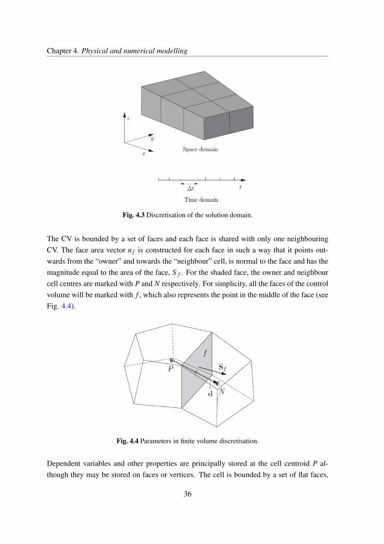
Chapter 4. Physical and numerical modelling
Fig. 4.3 Discretisation of the solution domain.
The CV is bounded by a set of faces and each face is shared with only one neighbouringCV. The face area vector n f is constructed for each face in such a way that it points out-wards from the “owner” and towards the “neighbour” cell, is normal to the face and has themagnitude equal to the area of the face, S f . For the shaded face, the owner and neighbourcell centres are marked with P and N respectively. For simplicity, all the faces of the controlvolume will be marked with f , which also represents the point in the middle of the face (seeFig. 4.4).
Fig. 4.4 Parameters in finite volume discretisation.
Dependent variables and other properties are principally stored at the cell centroid P al-though they may be stored on faces or vertices. The cell is bounded by a set of flat faces,
36

Chapter 4. Physical and numerical modelling 4.4 Physical model
given the generic label f . In OpenFOAM there is no limitation on the number of facesbounding each cell, nor any restriction on the alignment of each face. This kind of meshis often referred to as “arbitrarily unstructured” to differentiate it from meshes in which thecell faces have a prescribed alignment, typically with the coordinate axes.Detailed descriptions of its implementation can be found in Versteeg and Malalasekera(1995), Ferziger and Peric (1999) and Ubbink (1997). Details of the pressure-velocity cou-pled algorithm and volume of fluid method implemented in OpenFOAM are presented inAppendix D and E.
4.4.2 Hydrodynamic modelling of semi-submersible FOWT concept
A forced harmonic vertical motion of a rigid body, with amplitude A and frequency ω,centered in the coordinate z0 (see Fig. 4.2):
z(t) = z0+A sin(ωt), (4.28)
is considered.It is assumed that the two parameters that govern the small amplitude oscillating flow in-duced by the heave oscillation of a structure are the Keulegan-Carpenter number (KC) andthe frequency parameter (β):
KC = 2πA
Dd, (4.29)
β =D2
d f
ν, (4.30)
where f is the frequency in Hz of the oscillation, Dd is the disc diameter and ν is thekinematic viscosity of the fluid. Discussion of these parameters can be found in Keuleganand Carpenter (1958) and Sarpkaya and Isaacson (1981). One can obtain a Reynolds numberbased on the oscillation velocity of the disc as:
Re = KC ·β =A ω Dd
ν. (4.31)
In addition, the elevation ratio h/rd is considered to have an effect on the added mass anddamping coefficients when the disc oscillates close to the seabed. Under these assumptions,in non-dimensional terms, the hydrodynamic coefficients are functions of KC, β and h/rd.For a heave plate oscillating in heave, the added mass is approximately equal to the mass offluid contained in an imaginary sphere of the same radius as the disc and the natural heave
37
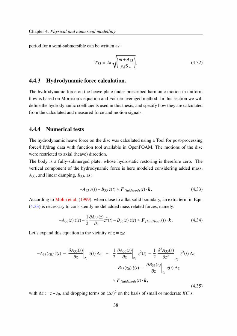
Chapter 4. Physical and numerical modelling
period for a semi-submersible can be written as:
T33 = 2π
√(m+A33
ρgS w
), (4.32)
4.4.3 Hydrodynamic force calculation.
The hydrodynamic force on the heave plate under prescribed harmonic motion in uniformflow is based on Morrison’s equation and Fourier averaged method. In this section we willdefine the hydrodynamic coefficients used in this thesis, and specify how they are calculatedfrom the calculated and measured force and motion signals.
4.4.4 Numerical tests
The hydrodynamic heave force on the disc was calculated using a Tool for post-processingforce/lift/drag data with function tool available in OpenFOAM. The motions of the discwere restricted to axial (heave) direction.The body is a fully-submerged plate, whose hydrostatic restoring is therefore zero. Thevertical component of the hydrodynamic force is here modeled considering added mass,A33, and linear damping, B33, as:
−A33 z(t)−B33 z(t) ≈ F f luid/body(t) · k . (4.33)
According to Molin et al. (1999), when close to a flat solid boundary, an extra term in Eqn.(4.33) is necessary to consistently model added mass related forces, namely:
−A33(z) z(t)−12∂A33(z)∂z
z2(t)−B33(z) z(t) ≈ F f luid/body(t) · k . (4.34)
Let’s expand this equation in the vicinity of z = z0:
−A33(z0) z(t) −∂A33(z)∂z
∣∣∣∣∣z0
z(t) ∆z −12∂A33(z)∂z
∣∣∣∣∣z0
z2(t) −12∂2A33(z)∂z2
∣∣∣∣∣∣z0
z2(t) ∆z
− B33(z0) z(t) −∂B33(z)∂z
∣∣∣∣∣z0
z(t) ∆z
≈ F f luid/body(t) · k ,(4.35)
with ∆z := z− z0, and dropping terms on (∆z)2 on the basis of small or moderate KC’s.
38

Chapter 4. Physical and numerical modelling 4.4 Physical model
If Eqn. (4.35) is multiplied by z and integrated over one period, the following expression isobtained:
∫ t+T
tA33(z0) z2(t)dt +
12
∫ t+T
t
∂2A33(z)∂z2
∣∣∣∣∣∣z0
z2(t) ∆z z(t)dt
=
∫ t+T
tz(t) · Fbody/ f luid(t) · kdt .
(4.36)
This equation has been solved iteratively for each case, neglecting the second order deriva-tive term in the first iteration, and incorporating it after its estimation from A33(z) obtainedin the first iteration, and so on. It has been found that, in all cases analyzed, the weight ofthe second order derivative term in the equation is basically negligible.
On the other hand, if Eqn. (4.35) is multiplied by z(t) and integrated over one period, B33
can be directly obtained since only one summand survives in the projection:
B33 =
∫ t+Tt z(t) · Fbody/ f luid(t) · kdt∫ t+T
t z2(t)dt. (4.37)
Taking into account that vB = z · k , this expression can be written as:
B33 =
∫ t+Tt vB(t) · Fbody/ f luid(t)dt∫ t+T
t v2B(t)dt
. (4.38)
Substituting into Eqn. (4.27), we get an approximation of the linear damping coefficientfrom the analysis of the flow vorticity field, expressed as:
B33ω :=
∫ t+Tt Eω dt∫ t+T
t v2B(t)dt
. (4.39)
Thus we have obtained an explicit expression relating the global damping coefficient withthe rate of change of enstrophy.
4.4.5 Experimental tests
In the case of experiments, the hydrodynamic force F f luid/body(t) is then given by prop-erly subtracting the body inertia force, FI(t), and the hydrostatic restoring, FK(t), from the
39

Chapter 4. Physical and numerical modelling
measured force Fmeas(t). That is:
F f luid/body(t) = Fmeas(t)−FI(t)−FK(t), (4.40)
FI(t) = −zω21m, (4.41)
FK(t) = −zS wρg. (4.42)
The heave added mass A33 and damping coefficient B33 of the heave plate are calculatedfrom the corresponding selected time history of the total force F f luid/body(t) (Eqn. 4.40),velocity z(t), acceleration z(t) and displacement z(t) using a fourier projection method andby expressing the force as in the Eqn. (4.43). We can assume that the hydrodynamic forcemay be represented by a linear combination of acceleration and velocity signals.
−B33 · z(t)−A33 · z(t) = F f luid/body(t). (4.43)
The hydrodynamic coefficients are defined as follow, (Wadhwa et al., 2010):
A33 =Fbody/ f luid,1 cos(φ)
ω2A, (4.44)
B33 =Fbody/ f luid,1 sin(φ)
ωA, (4.45)
where Fbody/ f luid,1 and A are the magnitudes of the first harmonic component in the forceand displacement respectively, φ is the phase angle between the force and the heave platemotion.
The added mass coefficient is based on the force in phase with acceleration normalized withrespect to the mass of the displaced water and the acceleration amplitude of the harmonicoscillation, ω2 A, and the damping coefficient is based on the force in phase with velocity.
Hydrodynamic coefficients (from numerical and experimental results) are presented in theirnon-dimensional form, as follows:
Ca =A33
Ma, (4.46)
Cb =B33
ωMa, (4.47)
where Ma is the added mass in an unbounded fluid, defined as Ma = 8/3 ρ r3d, (Sarpkaya and
40
Chapter 4. Physical and numerical modelling 4.4 Physical model
Isaacson, 1981).
4.4.6 Numerical model of turbulence
Since early last century, a number of turbulence models have been developed to improvethe performance of numerical simulations for a large variety of different two or three di-mensional flow problems especially at high Reynolds numbers. The central concept is toaverage the governing equations over a time or space scale so that the resultant equationsdescribe the distribution of the mean velocity and pressure in the flow. This is acceptablefrom an engineering point of view since the mean motion rather than the details of thefluctuating motion is of primary interest for engineers in most practical calculations. Theintroduction of turbulence models serves to provide closure to the time or space averagedgoverning equations which contain unknown terms representing the transport of turbulentmotion.Numerical calculation of the springing damping of a single cylinder was performed by Huseand Utnes (1994) and Utnes et al. (1995). The axisymmetric numerical model is basedon Reynolds equations with a one-equation turbulence closure. A Galerkin finite elementmethod is used to solve the equations. For the momentum equations a fractional step formu-lation is applied. An intermediate velocity is first computed by neglecting the pressure, thepressure field is then computed from a Poisson equation, and the velocity field is finally cor-rected by including the pressure effect. The intermediate velocity and the turbulence equa-tions are computed using a weak form of the characteristics method. No distinct differenceamong the results of laminar and turbulence modelling was found from the calculations.There is good agreement among the previous investigations that the boundary layer is ex-pected to be laminar in model scale as well as prototype TLP in springing oscillations dueto their very small amplitudes (Huse and Utnes, 1994). Therefore, in the present study, thenumerical calculations of viscous damping of heave plates configurations are based on theNavier-Stokes formulation, omitting any turbulence modelling.Prislin et al. (1998) examined how the added mass and drag coefficients of a solid square-plate in infinite fluid vary with the Reynolds number (the width of the plate being the charac-teristic length) and with the KC number. Their conclusion was that the added mass of solidplates does not depend on the Reynolds number and that the drag coefficient at Reynoldsnumbers higher than 105 does not vary significantly with Reynolds number.The Reynolds number of the present simulations is large and therefore significant turbulencemay develop. However, the boundary layer separation takes place at a known location (theplate edge), and the size of the vortical structures is relatively large (of the order of themotion amplitude) and, hence, unsensitive to subgrid RANS modelling. For these reasons,
41
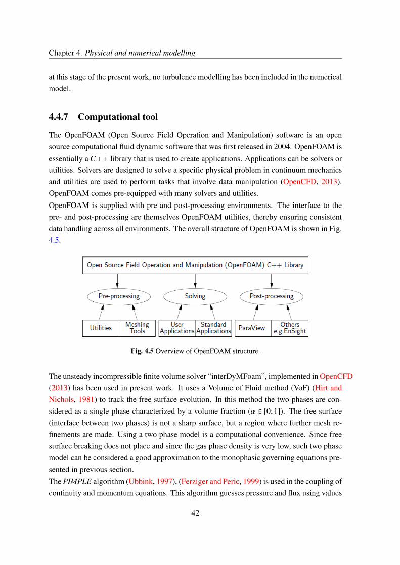
Chapter 4. Physical and numerical modelling
at this stage of the present work, no turbulence modelling has been included in the numericalmodel.
4.4.7 Computational tool
The OpenFOAM (Open Source Field Operation and Manipulation) software is an opensource computational fluid dynamic software that was first released in 2004. OpenFOAM isessentially a C++ library that is used to create applications. Applications can be solvers orutilities. Solvers are designed to solve a specific physical problem in continuum mechanicsand utilities are used to perform tasks that involve data manipulation (OpenCFD, 2013).OpenFOAM comes pre-equipped with many solvers and utilities.OpenFOAM is supplied with pre and post-processing environments. The interface to thepre- and post-processing are themselves OpenFOAM utilities, thereby ensuring consistentdata handling across all environments. The overall structure of OpenFOAM is shown in Fig.4.5.
Fig. 4.5 Overview of OpenFOAM structure.
The unsteady incompressible finite volume solver “interDyMFoam”, implemented in OpenCFD(2013) has been used in present work. It uses a Volume of Fluid method (VoF) (Hirt andNichols, 1981) to track the free surface evolution. In this method the two phases are con-sidered as a single phase characterized by a volume fraction (α ∈ [0;1]). The free surface(interface between two phases) is not a sharp surface, but a region where further mesh re-finements are made. Using a two phase model is a computational convenience. Since freesurface breaking does not place and since the gas phase density is very low, such two phasemodel can be considered a good approximation to the monophasic governing equations pre-sented in previous section.The PIMPLE algorithm (Ubbink, 1997), (Ferziger and Peric, 1999) is used in the coupling ofcontinuity and momentum equations. This algorithm guesses pressure and flux using values
42

Chapter 4. Physical and numerical modelling 4.4 Physical model
from the previous time step, and uses momentum equation in order to find the velocity. Anequation, obtaining the pressure, is then solved and fluxes are finally corrected in order tosatisfy continuity. All steps must be repeated until convergence task is achieved.The schemes implemented for both convection divergence and laplacian terms were thebounded vanLeer limiter (but to produce smoother interfaces in this work the specialised in-terfaceCompression scheme will be used) and the unbounded second order linear corrected,respectively were used. The first time derivative term of the transient time scheme imple-mented in this model used the Euler scheme, which is the first order, bounded and implicitscheme available in OpenFOAM for solving ordinary differential equations (OpenCFD,2013). The generalised geometric algebraic multi-grid (GAMG) were used to discretizedpressure and cell displacement, and smoother GaussSeidel to discretized velocity governingequations.It is important to underline that results obtained by the application of numerical methodmust be independent from the grid used in the calculation. For this reason a mesh have tobe fine enough in order to evaluate the variation in space of variables, but it must be takeninto account that computational efforts grow up with the growth of the number of cells. Thenext Chapters (5 and 6) shown the convergence analysis, both in time and mesh generationfor each study case analyzed in this work.
4.4.8 Validation of numerical procedure
The validation of the numerical model has been carried out in three stages. First, a com-parison of the calculated damping ratio with the experimental results of Thiagarajan andTroesch (1998) for a cylinder + disc configuration was done, second, the same was done forthe experimental work done by Wadhwa et al. (2010), and third, flow pattern comparisonswith the flow visualization experiments of He et al. (2008) were conducted. Details of anextensive convergence studies and mesh definition can be found in Garrido-Mendoza et al.(2013).In the first stage, the damping ratios from Thiagarajan and Troesch (1998) are taken asreference. The damping ratio allows for the dependence of the viscous damping on thegeometry of the disc to be examined. The damping ratio can be defined as:
Z =1
3 π2 CGCd
CmKC , (4.48)
where CG is a geometric constant depending on the geometry of the cylinder + disc config-uration, Cd and Cm = 1+Ca are the drag coefficient and the inertia coefficient, respectively,calculated from time history force. More details of the formulation can be found in Thia-
43

Chapter 4. Physical and numerical modelling
garajan and Troesch (1998). Fig. 4.6 shows the results of the damping ratio of the cylinder+ disc configuration at different amplitudes of oscillation and a good agreement is seenbetween the experimental and numerical data.
0 0.1 0.2 0.3 0.4 0.5 0.60
0.005
0.01
0.015
0.02
0.025
0.03
Da
mp
ing
ra
tio−
Z
KC
Present work.Thiagarajan & Troesch (1998).
Fig. 4.6 Damping ratio Z vs. KC for a cylinder with disc using Eqn. (4.48).
The second set of validation simulations were aimed at numerically reproducing the experi-mental work done by Wadhwa et al. (2010) for a solid disc 200 mm in diameter, 2 mm thick,oscillating at amplitudes varying from 1 to 48 mm and an elevation h of the disc from theseabed varying between 0.2 and 2 times the disc radius. Figs. 4.7(a) and 4.7(b) show acomparison with the published experimental data of Wadhwa et al. (2010), Vu et al. (2008)and Tao and Dray (2008) for different KC ranges. Our results for added mass and dampingshow similar behaviour to the curves obtained by Tao and Dray (2008).Fig. 4.7(a) presents a larger Ca value for simulations in comparison to experiments, althoughthe behaviour for smaller KC tends to the theoretical value, which does not happen in ex-periments of Wadhwa et al. (2010). Some differences could be attributed to the fact that allexperiments were conducted in a finite volume of fluid (e.g. Wadhwa et al. (2010) work wasconducted in a 1 m3 tank). Some effects of the flow recirculating in the tank could have con-tributed to the difference. Furthermore, some experimental values were consistently higherthan others, pointing to some calibration or zeroing errors.Compared to flow visualization based on experiments, flow visualization based on wellvalidated numerical procedures can provide more details about the flow field, which canbe useful in order to understand the mechanisms of vortex shedding. Fig. 4.8 shows acomparison between present numerical simulations and the experiments performed by Heet al. (2008). The frames have been evenly spaced over one period starting at top dead
44

Chapter 4. Physical and numerical modelling 4.4 Physical model
0 0.2 0.4 0.6 0.8 1 1.2 1.4 1.6 1.8 21
1.2
1.4
1.6
1.8
2
2.2
2.4
KC
Ca
Numerical results. Seabed h/rd = 2.0.
Numerical results. Free Surface s/rd = 2.0.
Wadhwa & Thiagarajan (2009).
Vu et al. (2008).
Tao & Dray (2008).
(a) Added mass coefficient Ca using Eqn. (4.46).
0 0.2 0.4 0.6 0.8 1 1.2 1.4 1.6 1.8 20.2
0.4
0.6
0.8
1
1.2
1.4
1.6
1.8
KC
Cb
Numerical results. Seabed h/rd = 2.0.
Numerical results. Free Surface s/rd = 2.0.
Wadhwa & Thiagarajan (2009).
Vu et al. (2008).
Tao & Dray (2008).
(b) Damping coefficient Cb using Eqn. (4.47).
Fig. 4.7 Comparison of numerical and experimental added mass and damping coefficients for anoscillating heave plate.
centre (TDC). The results have been obtained with a disc whose thickness-diameter ratio istd/Dd = 1/87.5 and forced to oscillate sinusoidally in calm water, with a KC number of0.16. Qualitatively, the agreement between experiments and simulations, in the location ofthe vortical structures, can be considered reasonable.
45
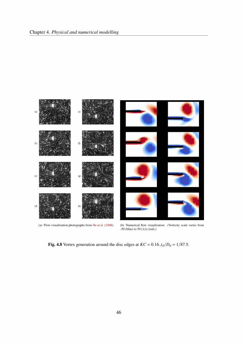
Chapter 4. Physical and numerical modelling
(a) Flow visualization photographs from He et al. (2008). (b) Numerical flow visualization. (Vorticity scale varies from-50 (blue) to 50 (1/s) (red).)
Fig. 4.8 Vortex generation around the disc edges at KC = 0.16 , td/Dd = 1/87.5.
46

Chapter 5
Parametric dependence of hydrodynamiccoefficients of a heave plate oscillatingnear a seabed or a free surface
5.1 Heave plate moving near a seabed
5.1.1 Introduction
This section is dedicated to the hydrodynamics of an oscillating heave plate close to theseabed. This problem is not directly related to the installations of floating offshore wind tur-bines, which is our main topic. However, it helps in understanding how the hydrodynamicof the heave plates is modified when getting closer to a fluid domain boundary. This bound-ary (the seabed) is theoretically simpler than the free surface (moving boundary) because itis fixed.If a body is moving in a fluid close to other bodies (moving or not), then its added mass anddamping differ from the added mass and damping corresponding to motion in an infinitefluid. This difference arises due to different boundary conditions: for an isolated body in aninfinite fluid one has only a boundary condition (impenetrability) on the body surface anda boundary condition at infinity. In the presence of other bodies one should also imposeboundary conditions on their surfaces.In some offshore applications such as deployment of foundation templates and subsea struc-tures, the penetration of a structure through the water surface and through the water columnare important stages. Publications (Cermelli et al., 2003; Roveri et al., 1996) discuss theloads on the crane wire during deployment of a subsea equipment. More recently, Thurstonet al. (2011) have discussed simplified mathematical models for statistical estimates of slack
47

Chapter 5. Parametric dependence
and snap loads on the crane wire, due to sudden changes in the net load on the wire. Thistypically happens when the difference between the hydrostatic and hydrodynamic loadschanges sign, i.e. crosses the zero value. The hydrodynamic load is strongly dependent onthe hydrodynamic coefficients of the structure being deployed. It is well-known that hydro-dynamic properties get altered significantly in the presence of a surface, hence requiring theuse of the method of images. Other studies, summarized in Sumer and Fredsøe (1997), onflow past pipelines on a seabed reveals that the vortex street formation is altered significantlyby the presence of a seabed. The Strouhal number is increased when a cylinder is close to asurface, and the effect of the wall is negligible at about 1.5 diameters.A practical application of such a situation is the motion of a heave plate near a seabed. Inthis work the seabed was simulated as a solid wall. The numerical results are compared withthe experiments conducted by Wadhwa et al. (2010).
5.1.2 Case study description
Forced numerical oscillations have been conducted in order to investigate the heave responseof a solid disc. The disc is oscillated at varying distances from the seabed (see Fig. 5.1) anddifferent amplitudes are applied, represented by the Keulegan-Carpenter parameter KC, asshown in Table 5.1. The Reynolds number range used is also documented.
Fig. 5.1 Disc elevation (h) from the seabed. rd is disc radius.
Fig. 5.2 shows the domain characteristics and the boundary conditions imposed for the casewhen the heave plate is oscillating near seabed. It is important to note that the seabed in oursimulations is impermeable, and that the simulations considered the flow as laminar, henceno turbulence model was used.
48
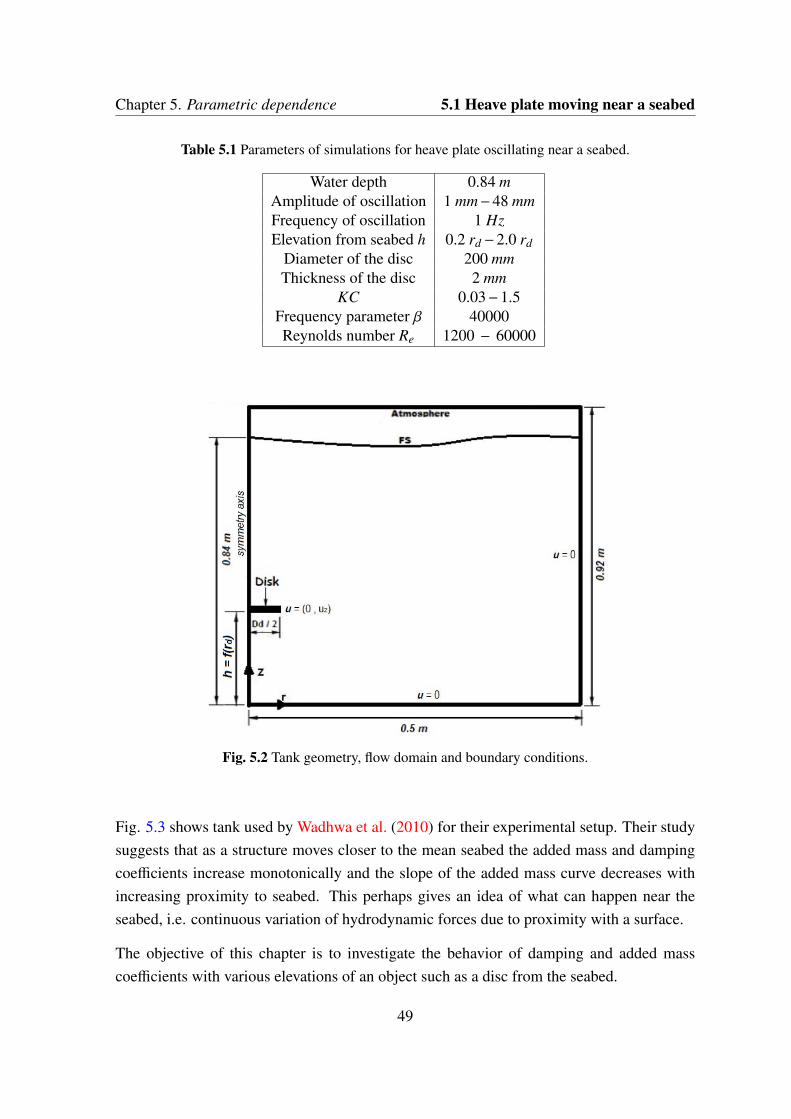
Chapter 5. Parametric dependence 5.1 Heave plate moving near a seabed
Table 5.1 Parameters of simulations for heave plate oscillating near a seabed.
Water depth 0.84 mAmplitude of oscillation 1 mm−48 mmFrequency of oscillation 1 HzElevation from seabed h 0.2 rd −2.0 rd
Diameter of the disc 200 mmThickness of the disc 2 mm
KC 0.03−1.5Frequency parameter β 40000Reynolds number Re 1200 − 60000
Fig. 5.2 Tank geometry, flow domain and boundary conditions.
Fig. 5.3 shows tank used by Wadhwa et al. (2010) for their experimental setup. Their studysuggests that as a structure moves closer to the mean seabed the added mass and dampingcoefficients increase monotonically and the slope of the added mass curve decreases withincreasing proximity to seabed. This perhaps gives an idea of what can happen near theseabed, i.e. continuous variation of hydrodynamic forces due to proximity with a surface.
The objective of this chapter is to investigate the behavior of damping and added masscoefficients with various elevations of an object such as a disc from the seabed.
49

Chapter 5. Parametric dependence
Fig. 5.3 Experiment set up in experiments conducted by Wadhwa et al. (2010).
5.1.3 Mesh generation
Due to the axisymmetric flow assumption, meshes for the simulation of the flow induced bythe oscillating vertical cylinder are generated in a 2D region. The geometrical characteristicsof the analyzed moving body (cylinder + heave plate) allow us to use quadrilateral structuredmeshes, which facilitate the convergence analysis.
Since the amplitudes of oscillations are relatively small, the vortex patterns around the cylin-der are expected to depend only on the local flow around the sharp edge of the heave plate,flaps and holes.
The small regions around these elements, where the vortices are generated and shed dur-ing the oscillation, are resolved with more resolution by clustering the grid points in these
50
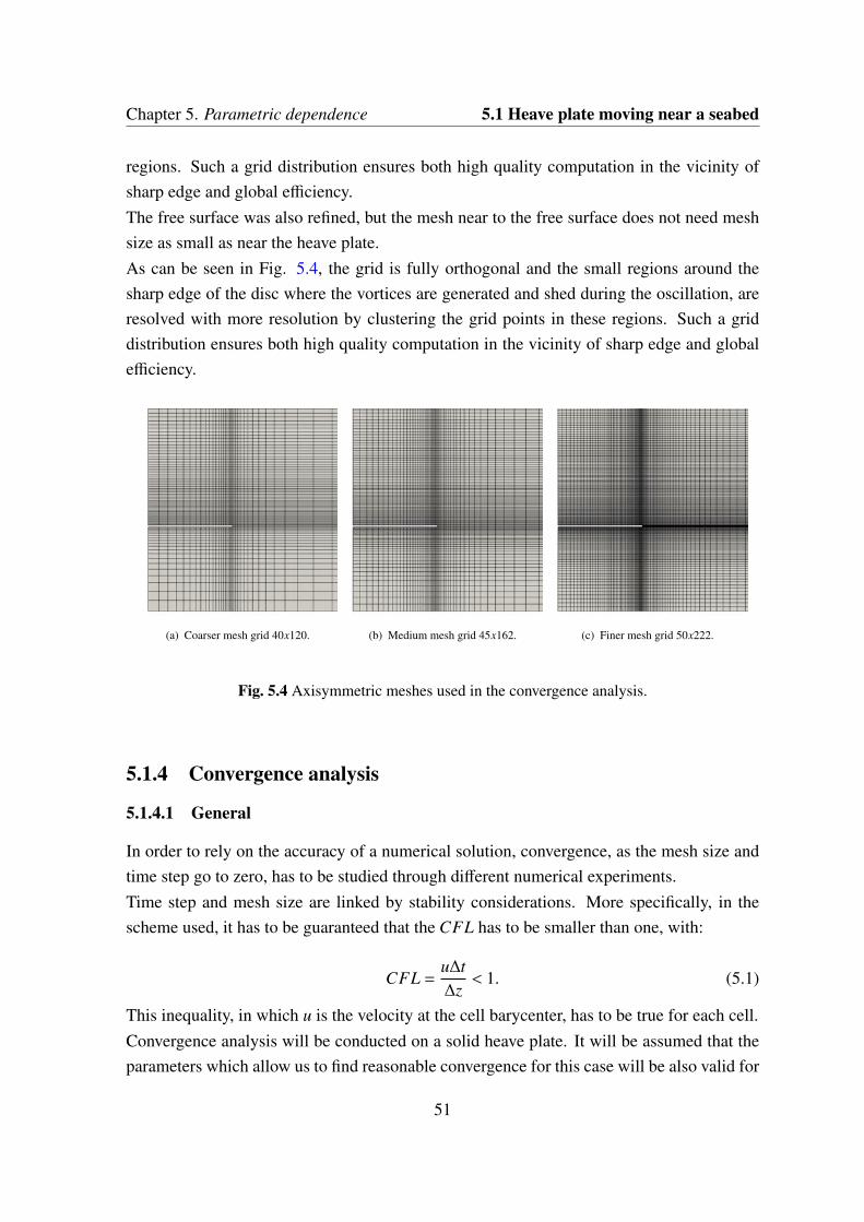
Chapter 5. Parametric dependence 5.1 Heave plate moving near a seabed
regions. Such a grid distribution ensures both high quality computation in the vicinity ofsharp edge and global efficiency.The free surface was also refined, but the mesh near to the free surface does not need meshsize as small as near the heave plate.As can be seen in Fig. 5.4, the grid is fully orthogonal and the small regions around thesharp edge of the disc where the vortices are generated and shed during the oscillation, areresolved with more resolution by clustering the grid points in these regions. Such a griddistribution ensures both high quality computation in the vicinity of sharp edge and globalefficiency.
(a) Coarser mesh grid 40x120. (b) Medium mesh grid 45x162. (c) Finer mesh grid 50x222.
Fig. 5.4 Axisymmetric meshes used in the convergence analysis.
5.1.4 Convergence analysis
5.1.4.1 General
In order to rely on the accuracy of a numerical solution, convergence, as the mesh size andtime step go to zero, has to be studied through different numerical experiments.Time step and mesh size are linked by stability considerations. More specifically, in thescheme used, it has to be guaranteed that the CFL has to be smaller than one, with:
CFL =u∆t∆z< 1. (5.1)
This inequality, in which u is the velocity at the cell barycenter, has to be true for each cell.Convergence analysis will be conducted on a solid heave plate. It will be assumed that theparameters which allow us to find reasonable convergence for this case will be also valid for
51

Chapter 5. Parametric dependence
the rest of simulations. The rationale behind this hypothesis is that the flow characteristicsare similar as well as the forces and integral quantities.The parameter to check convergence will be the drag coefficient Cd, that is obtained from aforce time history by Fourier analysis (Sarpkaya and Isaacson, 1981):
Cd = −3ωosc
4ρS A2ω2osc
∫ T
0F(t)cos(ωosc t)dt, (5.2)
where S is the projected area of the heave plate in the direction of the flow.
5.1.4.2 Convergence in mesh size
5.1.4.2.1 General. The numerical results of force and drag coefficient, obtained fromdifferent meshes for KC = 1.0, β = 40000 and ∆t = 1e−4s are presented in Fig. 5.5. It hasbeen checked that CFL < 1 with this ∆t for all cases analyzed.The details of the corresponding mesh parameters are listed in Table 5.2.
Table 5.2 Test cases for the influence of the meshes.
Mesh Total number of cellsCoarser mesh 40 x 120 4800
Coarser-Medium mesh 40 x 152 6080Medium mesh 45 x 162 7290
Medium-Finer mesh 45 x 187 8415Finer mesh 50 x 197 9850
Much Finer mesh 50 x 222 11100
Fig. 5.5 shows graphs that represent the force history and drag coefficient (Eqn. (5.2))calculated for the different mesh grid.As can be seen in the Fig. 5.5(a), the force amplitudes converge quickly. The finest meshseems to present a smoother shape which is related with a force more concentrated in thefrequency of the motion. Fig. 5.5(b) shows good convergence results when the mesh gridincreases.
5.1.4.2.2 Near wall treatment. Near-wall regions, where boundary layers occur, presentlarger gradients in the solution variables, and momentum and other scalar transports occurmost vigorously. These regions are made up of three zones (with their corresponding wally+) (Salim and Cheah, 2009), namely the:
• Viscous sublayer (y+ < 5)
52

Chapter 5. Parametric dependence 5.1 Heave plate moving near a seabed
18 19 20 21 22 23 24 25 26 27−12
−10
−8
−6
−4
−2
0
2
4
6
8
10
12
14
t [s]
~ Fbody/fluid(t)
[N]
40x120 cells40x152 cells45x162 cells45x187 cells50x197 cells50x222 cells
(a) Force history convergence with ∆t = 1e−4.
40x120 40x152 45x162 45x187 50x197 50x2224
5
6
7
8
9
10
Mesh grid [cells]
CD
(b) Drag coefficient convergence with ∆t = 1e−4 using Eqn. (5.2).
Fig. 5.5 Convergence tests in mesh sizes for h/rd = 2.0 and KC = 1.0.
• Buffer layer or blending region (5 < y+ < 30)
• Fully turbulent or log-law region (y+ > 30 to 60)
The non-dimensional wall distance for a wall-bounded flow y+ can be defined in the follow-ing way:
y+ =u∗yν
; (5.3)
53

Chapter 5. Parametric dependence
where u∗ is the friction velocity at the nearest wall, y is the distance to the nearest wall andν is the local kinematic viscosity of the fluid.For the finest mesh the computational y+ value, based on the cell size was approximately4.5, being within the viscous layer. It is in general recommended to have y+ < 1. In our casenot enough computational power is available to reach that limit. Nonetheless, as discussedin section 5.1.4.1, mesh convergence was reasonably good.Other estimation is given by Batchelor (1967) and used by Tao and Dray (2008) in a similarcontext. Batchelor found that for a circular cylinder of infinite length oscillating along itsaxis in a still fluid, the boundary layer thickness is:
δ =
√2νω. (5.4)
This characteristic length is chosen as the base of the the mesh sensitivity test. To predict theskin friction accurately, the condition that xmin/δ < 0.3 along the heave plate side surfacesis essential, which ensures that at least three mesh points are located in the boundary layerof cylinder side wall.Again, for the test cases with β = 40000, the value of the boundary layer thickness is δ =5.6419e−4 m and the minimum mesh spacing for all simulations was chosen as 2.5e−4 m.It indicates that the meshes used in this work and the minimum mesh spacing around theheave plate are good enough for the treatment of near-wall regions.Based on convergence tests, a mesh of 50 x 222 cells with a total number of cells equalto 11100 and minimum mesh spacing of xmin = 2.5e−4m was constructed in such a waythat the node points are concentrated near the cylinder and disc surfaces and stretched outgradually.
5.1.4.3 Convergence in ∆t
The choice of the time step to be used in the calculations is not straightforward. An im-portant consideration is the accuracy of the schemes with which the governing equationsare discretized in time. A smaller time step or, equivalently, a higher-order integration pro-cedure increases this accuracy. Balanced against this is the of computational time, whichincreases and may lead the computation to be too expensive. Stability is in principle guar-anteed on the basis of the CFL monitoring, as aforementioned.In order to determine a suitable time step, a number calculations for different time stepsare carried out. Fig. 5.6(a) shows a comparison between forces obtained for different timesteps, while Fig. 5.6(b) shows that the lowest time step considered may be required for theaccurate calculation of the drag coefficient.
54

Chapter 5. Parametric dependence 5.1 Heave plate moving near a seabed
17 18 19 20 21 22 23 24 25 26−15
−10
−5
0
5
10
15
~ Fbody/fluid(t)
[N]
t [s]
5.00 x 10⁻⁴ s2.00 x 10−4 s1.50 x 10−4 s1.25 x 10−4 s1.15 x 10−4 s1.00 x 10−4 s
(a) Forces obtained for different time step at KC = 1.0 and 50x222 cells.
1 1.5 2 2.5 3 3.5 4 4.5 5
x 10 −4
4
5
6
7
8
9
10
∆T [s]
CD
(b) Drag coefficient time step convergence at KC = 1.0 and 50x222 cells using Eqn. (5.2).
Fig. 5.6 Convergence tests in ∆t for h/rd = 2.0 and KC = 1.0.
Figure 5.6(a) shows how the discrepancies are mainly concentrated in the sharp of forcesand in the phase angle between them.
After this analysis, all the calculations were carried out with a mesh of 50 x 222 cells and atime step of ∆t = 1.0e−4s.
55
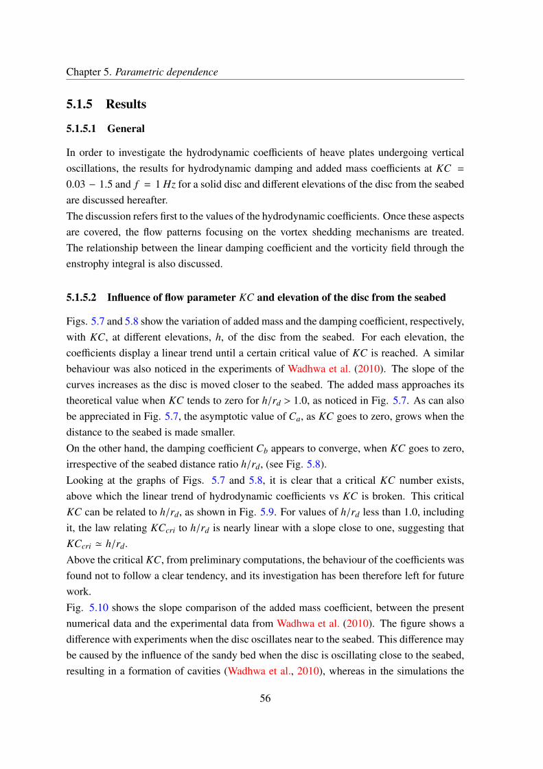
Chapter 5. Parametric dependence
5.1.5 Results
5.1.5.1 General
In order to investigate the hydrodynamic coefficients of heave plates undergoing verticaloscillations, the results for hydrodynamic damping and added mass coefficients at KC =0.03 − 1.5 and f = 1 Hz for a solid disc and different elevations of the disc from the seabedare discussed hereafter.The discussion refers first to the values of the hydrodynamic coefficients. Once these aspectsare covered, the flow patterns focusing on the vortex shedding mechanisms are treated.The relationship between the linear damping coefficient and the vorticity field through theenstrophy integral is also discussed.
5.1.5.2 Influence of flow parameter KC and elevation of the disc from the seabed
Figs. 5.7 and 5.8 show the variation of added mass and the damping coefficient, respectively,with KC, at different elevations, h, of the disc from the seabed. For each elevation, thecoefficients display a linear trend until a certain critical value of KC is reached. A similarbehaviour was also noticed in the experiments of Wadhwa et al. (2010). The slope of thecurves increases as the disc is moved closer to the seabed. The added mass approaches itstheoretical value when KC tends to zero for h/rd > 1.0, as noticed in Fig. 5.7. As can alsobe appreciated in Fig. 5.7, the asymptotic value of Ca, as KC goes to zero, grows when thedistance to the seabed is made smaller.On the other hand, the damping coefficient Cb appears to converge, when KC goes to zero,irrespective of the seabed distance ratio h/rd, (see Fig. 5.8).Looking at the graphs of Figs. 5.7 and 5.8, it is clear that a critical KC number exists,above which the linear trend of hydrodynamic coefficients vs KC is broken. This criticalKC can be related to h/rd, as shown in Fig. 5.9. For values of h/rd less than 1.0, includingit, the law relating KCcri to h/rd is nearly linear with a slope close to one, suggesting thatKCcri ≃ h/rd.Above the critical KC, from preliminary computations, the behaviour of the coefficients wasfound not to follow a clear tendency, and its investigation has been therefore left for futurework.Fig. 5.10 shows the slope comparison of the added mass coefficient, between the presentnumerical data and the experimental data from Wadhwa et al. (2010). The figure shows adifference with experiments when the disc oscillates near to the seabed. This difference maybe caused by the influence of the sandy bed when the disc is oscillating close to the seabed,resulting in a formation of cavities (Wadhwa et al., 2010), whereas in the simulations the
56

Chapter 5. Parametric dependence 5.1 Heave plate moving near a seabed
0 0.2 0.4 0.6 0.8 1 1.2 1.4 1.6 1.8 21
1.2
1.4
1.6
1.8
2
2.2
Ca
KC
Deep Waterh = 2.0 rdh = 1.0 rdh = 0.5 rdh = 0.4 rdh = 0.3 rdh = 0.2 rd
Fig. 5.7 Comparison of the added mass coefficient at different elevations from the seabed usingEqn. (4.46).
0 0.2 0.4 0.6 0.8 1 1.2 1.4 1.6 1.8 20.2
0.4
0.6
0.8
1
1.2
1.4
1.6
Cb
KC
Deep Waterh = 2.0 rdh = 1.0 rdh = 0.5 rdh = 0.4 rdh = 0.3 rdh = 0.2 rd
Fig. 5.8 Comparison of the damping coefficient at different elevations from the seabed using Eqn.(4.47).
seabed has been modeled as a fixed solid wall.
In order to describe the dependence of Ca and Cb coefficients with the submergence and KCnumber, the slope and offset of the least square linear fitting of such coefficients have been
57
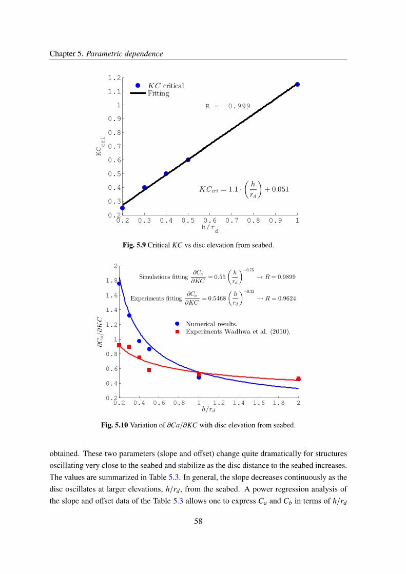
Chapter 5. Parametric dependence
0.2 0.3 0.4 0.5 0.6 0.7 0.8 0.9 10.2
0.3
0.4
0.5
0.6
0.7
0.8
0.9
1
1.1
1.2
KCcri
h/rd
R = 0.999
KCcri = 1.1 ·
(
h
rd
)
+ 0.051
KC criticalFitting
Fig. 5.9 Critical KC vs disc elevation from seabed.
0.2 0.4 0.6 0.8 1 1.2 1.4 1.6 1.8 20.2
0.4
0.6
0.8
1
1.2
1.4
1.6
1.8
2
∂C
a/∂KC
h/rd
Experiments fitting∂Ca
∂KC= 0.5468
(
h
rd
)
−0.32
→ R = 0.9624
Simulations fitting∂Ca
∂KC= 0.55
(
h
rd
)
−0.75
→ R = 0.9899
Numerical results.Experiments Wadhwa et al. (2010).
Fig. 5.10 Variation of ∂Ca/∂KC with disc elevation from seabed.
obtained. These two parameters (slope and offset) change quite dramatically for structuresoscillating very close to the seabed and stabilize as the disc distance to the seabed increases.The values are summarized in Table 5.3. In general, the slope decreases continuously as thedisc oscillates at larger elevations, h/rd, from the seabed. A power regression analysis ofthe slope and offset data of the Table 5.3 allows one to express Ca and Cb in terms of h/rd
58

Chapter 5. Parametric dependence 5.1 Heave plate moving near a seabed
for each KC value (see Eqn. (5.5) and (5.6)). These expressions can be used to evaluatethe added mass and damping near the seabed for ‘h/rd ≤ 2’. For larger elevation ratios,deep water condition is seen to be the best fit. Fig. 5.11 and 5.12 show the comparisonbetween the calculated coefficients and those fitted by Eqns. (5.5) and (5.6). The agreementis satisfactory.
Submergence Ca Cbh Slope (∂Ca/∂KC) Offset Slope (∂Cb/∂KC) Offset
2.0 rd 0.47 1.06 0.82 0.221.0 rd 0.56 1.10 1.00 0.230.5 rd 0.85 1.22 1.53 0.260.4 rd 1.01 1.30 1.80 0.280.3 rd 1.32 1.43 2.30 0.310.2 rd 1.87 1.72 3.23 0.39
Table 5.3 Slope and offset of curve fits for Ca and Cb.
Ca = 0.55(
hrd
)−0.75
KC+0.10
hrd
+1; (5.5)
Cb = 0.95(
hrd
)−0.55
KC+0.02
hrd
+0.2; (5.6)
1
1.2
1.4
1.6
1.8Added Mass at KC = 0.03
R = 0.99
Ca
Ca calculated
Ca fitting
1
1.2
1.41.6
1.8Added Mass at KC = 0.10
R = 0.99
Ca
0.2 0.4 0.6 0.8 1 1.2 1.4 1.6 1.8 21
1.21.41.61.8
2 Added Mass at KC = 0.20
R = 0.99
h/rd
Ca
Fig. 5.11 Variation of Ca with disc elevation from seabed for different KC numbers.
59

Chapter 5. Parametric dependence
0.2
0.3
0.4
0.5
0.6
Cb
Damping at KC = 0.10
0.2 0.4 0.6 0.8 1 1.2 1.4 1.6 1.8 20.2
0.4
0.6
0.8
1
Cb
Damping at KC = 0.20
h/rd
0.2
0.25
0.3
0.35
0.4
Cb
Damping at KC = 0.03
Cb calculated
Cb fitting
Fig. 5.12 Variation of Cb with disc elevation from seabed for different KC numbers.
In Fig. 5.13, the expression for Ca (Eqn. 5.5) has been compared with the results byMolin and Nielsen (2004) of potential flow around a porous oscillating disc, and with thewidespread use frequency domain potential flow software WAMIT, displaying fairly goodagreement. It has to be mentioned that Molin et al. (1999) and Vinje (2001) derived asymp-totic expressions for the added mass of a disc oscillating close to a solid wall. However,such formulae present small discrepancies that need to be sorted out before using them forcomparison. A future work thread about this topic has been included.Results of added mass and damping coefficients (Figs. 5.7 and 5.8) can also be madenon-dimensional with the aforementioned numerical values from WAMIT. With this non-dimensionalization, the offset difference between the curves is significantly reduced (seeFigs. 5.14 and 5.15), indicating, that the numerical results follow the potential flow pre-dictions. However, the ratios between the numerical results and the WAMIT values do notexactly tend to one for low KC values, something for which an explanation at this stage isyet missing. In these figures the KC values in the horizontal axis have been rescaled withthe proposed asymptotic value for critical KC, KC∗cri := h/rd. It is interesting to see how,with this rescaling, the abscissae of the points, for which the linear trend is broken, coincide.
60

Chapter 5. Parametric dependence 5.1 Heave plate moving near a seabed
0 0.1 0.2 0.3 0.4 0.5100
101
102
h/rd
A33/(8/3ρr3 d)
Present work: Eqn. [42] fitting
Molin & Nielsen (IWWWFB 2004)
Nielsen (2007). WAMIT
Fig. 5.13 Comparison of Ca between Eqn. (5.5), numerical values from WAMIT and analyticalresults of Molin and Nielsen (2004).
0 0.2 0.4 0.6 0.8 1 1.2 1.4 1.61.1
1.15
1.2
1.25
1.3
1.35
1.4
1.45
1.5
1.55
1.6
KC/KC∗
cri
A33/M
∗ a
h = 0.5 rdh = 0.4 rdh = 0.3 rdh = 0.2 rd
Fig. 5.14 Added mass coefficient for h/rd ≤ 0.5 non-dimensionalized with M∗a, with M∗a being thenumerical value from WAMIT.
61
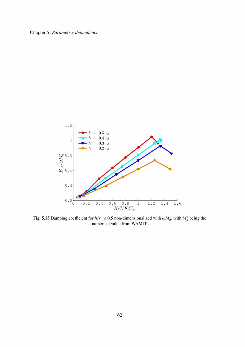
Chapter 5. Parametric dependence
0 0.2 0.4 0.6 0.8 1 1.2 1.4 1.60.2
0.4
0.6
0.8
1
1.2
KC/KC∗
cri
B33/ωM
∗ a
h = 0.5 rdh = 0.4 rdh = 0.3 rdh = 0.2 rd
Fig. 5.15 Damping coefficient for h/rd ≤ 0.5 non-dimensionalized with ωM∗a, with M∗a being thenumerical value from WAMIT.
62

Chapter 5. Parametric dependence 5.1 Heave plate moving near a seabed
5.1.5.3 Flow patterns analysis
5.1.5.3.1 General. Explanations for the behaviour of the hydrodynamic coefficients inproximity to the seabed ought to be obtained from examination of the flow features: whileadded mass modelling can be accurately achieved under the potential flow assumption(Molin et al., 1999), damping is more difficult to treat within that framework, althoughvery relevant results for simple configurations can be obtained (e.g. Graham (1980)). Thevariation of damping is normally attributed to flow separation and vortex shedding, and fullCFD analysis of the flow, is therefore, in principle, necessary to understand the dampingproperties of an oscillating body.
5.1.5.3.2 KC influence. Flow separation does not always result in vortex shedding (Faltin-sen, 1990). With increasing KC number, the transition from separation without vortex shed-ding to separation with vortex shedding should be visible. Clearly, this will also affect thedamping coefficient. When the KC number is small, the maximum displacement of particlesin the undisturbed flow is small compared to the scale of the body. It is therefore unfeasiblefor vortices to move far from the edge of the body from which they are shed, except underthe induced velocity field of other vortices.Fig. 5.16 shows, in frames equally spaced over one cycle, the distributions of the vorticity,where red denotes positive values and blue means negative. Half disc is shown, with thebottom of each frame indicating the position of the tank bottom. This is also the case for allfigures in this section.Results are presented for increasing KC values in panels a, b and c. For low and intermediateKC numbers, as the disc begins the descent (frames a1, b1), a dominant positive vortex (red)is created (frames a2, b2), which pairs with the negative vortex (blue) (frames a3, b3) in theupstroke, resulting in shedding of the vortex pair (frames a4, b4). When the disc reaches themaximum absolute displacement, the flow separates from the disc surface causing vortexshedding. Fig. 5.16(c) shows the instantaneous vorticity contours obtained at a higherKeulegan-Carpenter number, KC = 1.20. With this highest KC, the strength of the vorticesis much larger, due to the larger vorticity shed from the edges of the disc.In order to understand the meaning of the KC critical value, an analysis of the vorticitycontours for three cases with KC numbers just under, equal to, and just over the critical KCwas conducted. When the disc is oscillating just above the KC critical value, Fig. 5.17(c),entrapment of vortices by the seafloor (shown in blue in frame 1 of Fig. 5.17(c)) from earliercycles influences the shedding pattern and, thus, alters the force on the disc. In both Figs.5.17(a) and 5.17(b), such intense entrapment does not occur.
63

Chapter 5. Parametric dependence
(a) KC = 0.3. (b) KC = 0.5. (c) KC = 1.2.
Fig. 5.16 Vortex generation around disc close to seabed at h/rd = 1.0. (Vorticity scale varies from−25 s−1 (blue) to 25 s−1 (red).)
64

Chapter 5. Parametric dependence 5.1 Heave plate moving near a seabed
(a) Vortex generation around the disc atKC/KCcri = 0.96.
(b) Vortex generation around the disc atKC/KCcri = 1.00.
(c) Vortex generation around the disc atKC/KCcri = 1.04.
Fig. 5.17 Vortex generation around the disc at h/rd = 1.0. Blue lines indicate negative vorticity(initial condition: Top Dead Centre). Scale varies from −25 s−1(blue) to 25 s−1 (red).
65

Chapter 5. Parametric dependence
5.1.5.3.3 Influence of seabed distance ratio (h/rd). It is expected that the vortex shed-ding behaviour will be strongly dependent on the h/rd ratio.Fig. 5.18 shows the vortex patterns at a constant KC for three different height to radiusratios. Fig. 5.18(a) shows that the intensity of the vortices increases when reducing the h/rd
ratio, i.e., as the disc mean position is closer to the seabed.
5.1.5.4 Enstrophy dissipation term analysis
5.1.5.4.1 KC influence. Fig. 5.19 and 5.20 show the time history of the enstrophy term(Eqn. 4.20) for different amplitudes of oscillation corresponding, to the cases in Fig. 5.16.Actually, in Fig. 5.19, some labels indicate the instants of the selected frames shown inFigure 5.16(c).In order to make the curves comparable, Eqn. (4.27) shows that the enstrophy integral,Eω, is of the order of Fbody/ f luid · vB(t), in itself of the order of Cb ρ r3
d A2ω3. The factorρ r3
d A2ω3 has been therefore used to make Eω non-dimensional, a choice which shouldallow to establish comparisons with Cb tendencies.In order to estimate B33ω, these curves are integrated along one period, which means thatthe mean value is the crucial quantity. Such mean value is quite stable in time, as can beseen in Fig. 5.20. However, the ripples, whose rms amplitude is around 10% of the meanvalue, display a non-periodic behavior whose investigation has been left for future work.Looking at Figs. 5.19 and 5.20, it is clear that the mean values of the non-dimensionalenstrophy integral grows with KC number, an aspect which is consistent with the growth ofCb with KC (see Fig. 5.8).Figs. 5.21 and 5.22 show the time history of the enstrophy term at h/rd = 1 for KCs close tothe KC critical value. There is a clear variation in the behaviour of the curves when the discexceeds the critical value of KC, dissipating less energy, thus confirming the existence ofan amplitude in which the linear trend of the hydrodynamic coefficients is broken (see Figs.5.7 and 5.8).
5.1.5.4.2 Influence of seabed distance ratio (h/rd). It is also important to analyze theeffect that the seabed has on the dissipation term Eω. Figs. 5.23 and 5.24 show the en-strophy integral for different elevation ratios. They heuristically demonstrate that, in non-dimensional terms, the energy dissipation is larger when the elevation ratio, h/rd, is smaller,consistently with the Cb values shown in Fig. 5.8. This helps in clarifying the influence, onthe hydrodynamic coefficients, of the distance between the disc and the seabed.
66

Chapter 5. Parametric dependence 5.1 Heave plate moving near a seabed
(a) h/rd = 0.5. (b) h/rd = 1.0. (c) h/rd = 2.0.
Fig. 5.18 Vortex generation around the disc close to the seabed at KC = 0.5. (Scale varies from−25 s−1 (blue) to 25 s−1 (red).)
67
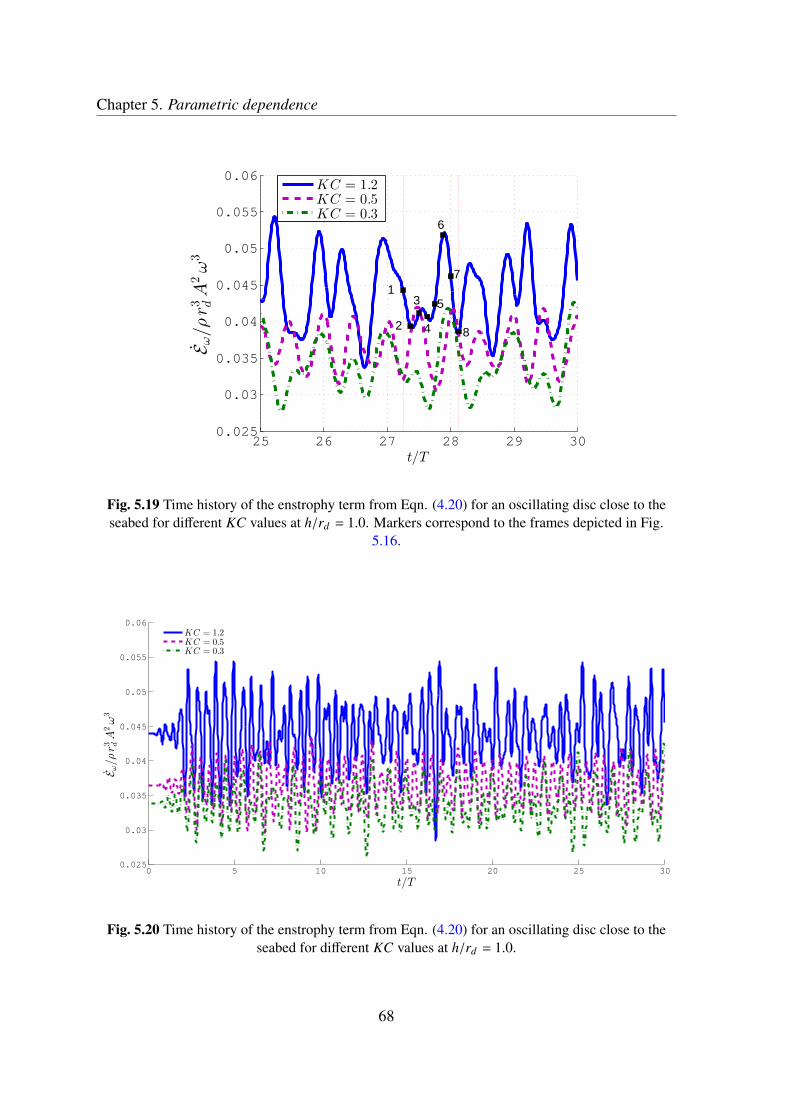
Chapter 5. Parametric dependence
25 26 27 28 29 300.025
0.03
0.035
0.04
0.045
0.05
0.055
0.06
t/T
Eω/ρ
r3 dA
2ω3
KC = 1.2KC = 0.5KC = 0.3
2
13 5
6
84
7
Fig. 5.19 Time history of the enstrophy term from Eqn. (4.20) for an oscillating disc close to theseabed for different KC values at h/rd = 1.0. Markers correspond to the frames depicted in Fig.
5.16.
0 5 10 15 20 25 300.025
0.03
0.035
0.04
0.045
0.05
0.055
0.06
t/T
Eω/ρ
r3 dA
2ω3
KC = 1.2KC = 0.5KC = 0.3
Fig. 5.20 Time history of the enstrophy term from Eqn. (4.20) for an oscillating disc close to theseabed for different KC values at h/rd = 1.0.
68
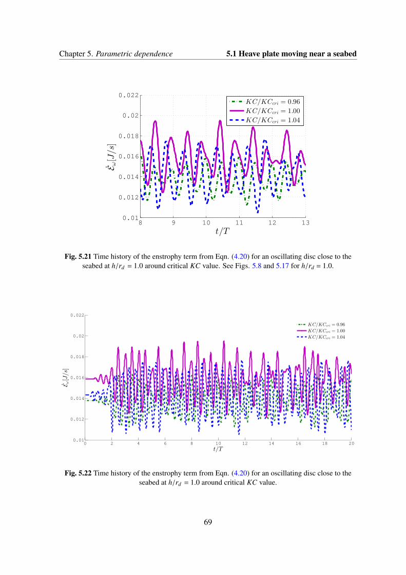
Chapter 5. Parametric dependence 5.1 Heave plate moving near a seabed
8 9 10 11 12 130.01
0.012
0.014
0.016
0.018
0.02
0.022
t/T
Eω[J/s]
KC/KCcri = 0.96
KC/KCcri = 1.00
KC/KCcri = 1.04
Fig. 5.21 Time history of the enstrophy term from Eqn. (4.20) for an oscillating disc close to theseabed at h/rd = 1.0 around critical KC value. See Figs. 5.8 and 5.17 for h/rd = 1.0.
0 2 4 6 8 10 12 14 16 18 200.01
0.012
0.014
0.016
0.018
0.02
0.022
t/T
Eω[J/s]
KC/KCcri = 0.96
KC/KCcri = 1.00
KC/KCcri = 1.04
Fig. 5.22 Time history of the enstrophy term from Eqn. (4.20) for an oscillating disc close to theseabed at h/rd = 1.0 around critical KC value.
69

Chapter 5. Parametric dependence
10 11 12 13 14 150.02
0.03
0.04
0.05
0.06
0.07
0.08
0.09
0.1
t/T
Eω/ρ
r3 dA
2ω3
h/rd = 0.4
h/rd = 0.5
h/rd = 1.0
h/rd = 2.0
Fig. 5.23 Time history of the enstrophy term from Eqn. (4.20) for an oscillating disc close to theseabed for different h/rd values at KC = 0.4.
0 5 10 15 20 25 300.02
0.03
0.04
0.05
0.06
0.07
0.08
0.09
0.1
t/T
Eω/ρ
r3 dA
2ω3
h/rd = 0.4
h/rd = 0.5
h/rd = 1.0
h/rd = 2.0
Fig. 5.24 Time history of the enstrophy term from Eqn. (4.20) for an oscillating disc close to theseabed for different h/rd values at KC = 0.4.
70

Chapter 5. Parametric dependence 5.1 Heave plate moving near a seabed
5.1.5.4.3 Comparison between B33 and B33ω. The relationship between the dampingcoefficient B33ω obtained through the enstrophy integral (Eqn. 4.39) and the damping co-efficient obtained with the classical forces projection approach (Eqn. 4.37), are discussedhereinafter. Figs. 5.25 − 5.27 show the comparison of the damping coefficient obtainedwith both approaches for three representative cases. The matching is, in general, very good.This indicates that the enstrophy contribution to the dissipation Eω may be the lead actor inthis type of flows.
0 0.2 0.4 0.6 0.8 1 1.2 1.40
0.2
0.4
0.6
0.8
1
1.2
1.4
1.6
KC
Cb
Enstrophy (Time Integral)Fourier projection
Fig. 5.25 Comparison of hydrodynamic damping coefficient (Cb) with B33 at h/rd = 1.0, obtainedwith the enstrophy integral (Eqn. (4.39)) and classical (Sarpkaya and Isaacson, 1981) Fourier
projection (Eqn. (4.47)), for an oscillating heave plate near a seabed.
71
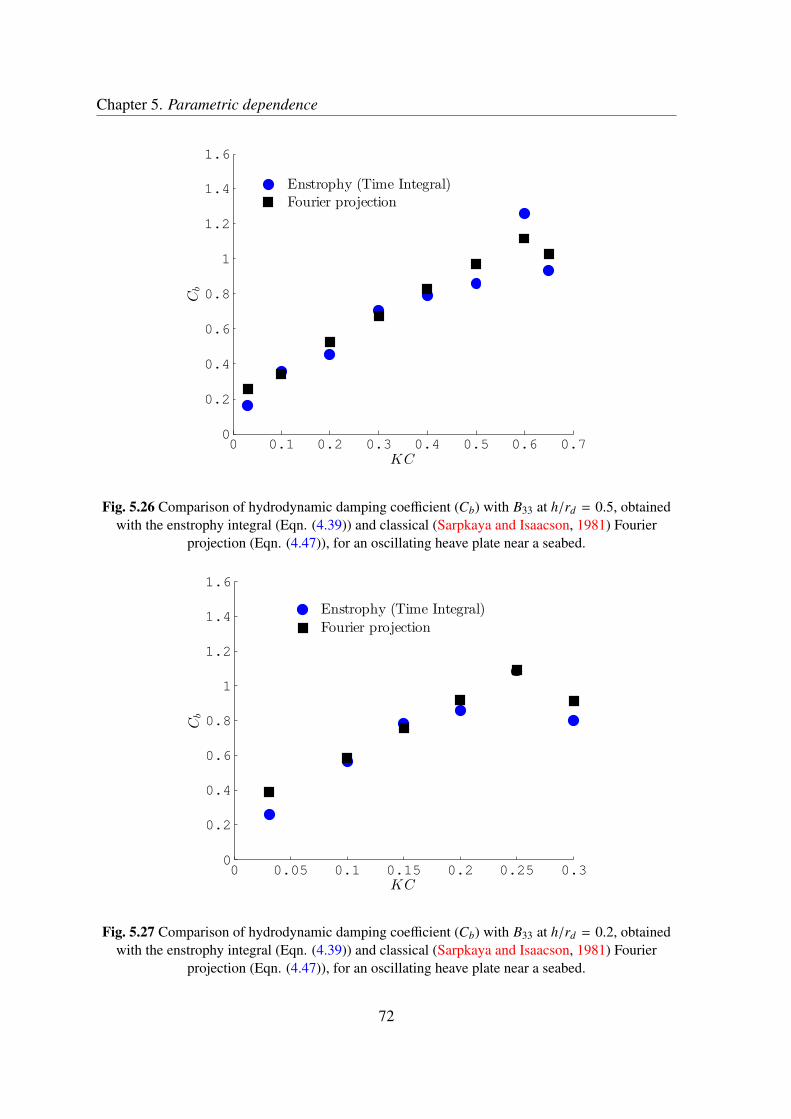
Chapter 5. Parametric dependence
0 0.1 0.2 0.3 0.4 0.5 0.6 0.70
0.2
0.4
0.6
0.8
1
1.2
1.4
1.6
KC
Cb
Enstrophy (Time Integral)Fourier projection
Fig. 5.26 Comparison of hydrodynamic damping coefficient (Cb) with B33 at h/rd = 0.5, obtainedwith the enstrophy integral (Eqn. (4.39)) and classical (Sarpkaya and Isaacson, 1981) Fourier
projection (Eqn. (4.47)), for an oscillating heave plate near a seabed.
0 0.05 0.1 0.15 0.2 0.25 0.30
0.2
0.4
0.6
0.8
1
1.2
1.4
1.6
KC
Cb
Enstrophy (Time Integral)
Fourier projection
Fig. 5.27 Comparison of hydrodynamic damping coefficient (Cb) with B33 at h/rd = 0.2, obtainedwith the enstrophy integral (Eqn. (4.39)) and classical (Sarpkaya and Isaacson, 1981) Fourier
projection (Eqn. (4.47)), for an oscillating heave plate near a seabed.
72

Chapter 5. Parametric dependence 5.2 Heave plate oscillating close to a free surface
5.2 Heave plate oscillating close to a free surface
5.2.1 Introduction
This section will study the hydrodynamic forces of the submerged heave plate oscillatingnear a free surface, and unlike the presence of a solid boundary (5.1), a free surface boundaryincrease considerably to the complexity of the problem.The flow induced by a body oscillating near a free surface of a fluid is significantly differentfrom that of an infinite fluid. The difference is due to the presence of a boundary condition(constancy of pressure) on the free surface. The free surface effect can strongly influencethe added mass and damping coefficient values as a function of the frequency when thesubmerged body oscillates near a free surface (Chung, 1977). Also the flow is highly non-linear even at very small amplitude of oscillation, when the body is slightly submerged.Any prior rotational or translational motion of those bodies would have generated free sur-face waves which would in turn affect the loading on the body. This represents the majorcomplication introduced by the presence of a free surface. It is however clear that if thebody motion is sufficiently slow (characterized by a velocity, U say), then the waves createdwill be negligibly small and these prior history effects would also be small (Brennen, 1982).
5.2.2 Case study description
Figure 5.28 shows the simulation setup and boundary conditions used in all cases in thissection. The no-flux and no-slip velocity boundary conditions are imposed along the os-cillatory body surface. The heave plates were forced to oscillate harmonically in a verticaldirection in quiescent water.The parameters for the simulations used in this section were listed in Table 5.1.
5.2.3 Mesh generation
A brief description of the mesh characteristics used in this case study is presented in Figure5.29. Mesh distribution and minimum cell size around the disc is the same to the mesh andparameters used in section 5.1.3. Here the refining of the free surface is also shown.
73

Chapter 5. Parametric dependence
Fig. 5.28 Disc submergence (s) from the free surface. rd is disc radius.
(a) Grid distribution of the domain. (b) Detail of the grid around the disc and the free sur-face.
Fig. 5.29 Axisymmetric mesh used for the disc oscillating close to the free surface cases.
74

Chapter 5. Parametric dependence 5.2 Heave plate oscillating close to a free surface
5.2.4 Results
5.2.4.1 General
Similar to the previous case (heave plates oscillating close to the sea-floor), the hydrody-namic coefficients of a heave plate oscillating in vertical direction at different submergencefrom the free surface are discussed hereafter.The results section refers first to the dependence of the hydrodynamic coefficients withthe amplitude of the motion and the submergence ratio. Then, vorticity and free-surfacevisualization is made in order to understand the flow features. Finally, the relationshipbetween the linear damping coefficient and the dissipation terms, Eω and EFS ,(Eqn. 4.20and 4.21), enstrophy and free surface dissipation, respectively, is discussed.
5.2.4.2 Influence of flow parameter KC and submergence of the disc from the freesurface
Figures 5.30 and 5.31 show the influence on the added mass and damping when the heaveplate is oscillating close to the free surface. As can be seen, the added mass first increasesat the acceleration of the fluid between the free surface and the body increases, but thendecreases when the depth is less than about one body dimension because less fluid is beingaccelerated.
0 0.2 0.4 0.6 0.8 1 1.2 1.4 1.6 1.8 21
1.2
1.4
1.6
1.8
2
Ca
KC
s = 2.0 rds = 1.0 rds = 0.5 rds = 0.4 rd
Fig. 5.30 Comparison of the added mass coefficient at different submergences from the free surfaceusing Eqn. (4.46).
75

Chapter 5. Parametric dependence
0 0.2 0.4 0.6 0.8 1 1.2 1.4 1.6 1.8 20.2
0.4
0.6
0.8
1
1.2
1.4
1.6
1.8
2
2.2
KC
Cb
s = 2.0 rds = 1.0 rds = 0.5 rds = 0.4 rd
Fig. 5.31 Comparison of the damping coefficient at different submergences from the free surfaceusing Eqn. (4.47).
The behaviour of the added mass when reach certain KC value as the disc approaches toa free surface was also observed in the case when the disc oscillates near the seabed. Fig.5.32 shows the relation of the critical KC and the s/rd ratio.
0 0.2 0.4 0.6 0.8 1 1.2 1.4 1.6 1.8 20
0.2
0.4
0.6
0.8
1
1.2
1.4
1.6
KCcri
s/rd
KCcri = 0.8 · ln
(
s
rd
)
+ 0.95
R = 0.995KC criticalFitting
Fig. 5.32 Critical KC vs disc submergence from free surface ‘s’.
In order to describe the dependence of Ca and Cb coefficients on the submergence and KCnumber, the slope and offset of the least square linear fitting of such coefficients have beenobtained. These two parameters (slope and offset) change quite dramatically for structures
76

Chapter 5. Parametric dependence 5.2 Heave plate oscillating close to a free surface
oscillating very close to the seabed and stabilize as the disc distance to the free surfaceincreases. The values are summarized in Table 5.4. In general, the slope decreases contin-uously as the disc oscillates at larger submergences, s/rd, from the free surface. A powerregression analysis of the slope and offset data of the Table 5.4 allows one to express Ca
and Cb in terms of s/rd for each KC value (see Eqn. (5.7) and (5.8)). These expressionscan be used to evaluate the added mass and damping for a disc oscillating closer to a freesurface. Figs. 5.33 and 5.34 show the comparison between the calculated coefficients andthose fitted by Eqns. (5.7) and (5.8). The agreement is satisfactory.
Table 5.4 Slope and offset of curve fits for Ca and Cb.
Submergence Ca Cbs Slope (∂Ca/∂KC) Offset Slope (∂Cb/∂KC) Offset
2.0 rd 0.70 1.04 0.63 0.221.0 rd 0.64 1.15 0.91 0.320.5 rd 0.86 1.44 1.98 0.620.4 rd 1.25 1.43 2.49 0.85
Ca = 0.90srd
−0.95KC+
0.15s
rd
+1; (5.7)
Cb = 1.25srd
−0.95KC+
0.15s
rd
+0.2; (5.8)
In order to validate the above expression for added mass (Eqn. 5.7), a comparison withpublished data is made in Fig. 5.35. Figure shows that the added mass obtained by presentwork differs from Greenhow’s data (non-dimensionalized with ρ π r2) for smaller submer-gences (s/rd ≪ 0.5) due to fact that Greenhow used a horizontal circular cylinder is hiswork, but both cases, when the disc or cylinder approach the free surface, the heave addedmass becomes infinite.
5.2.4.3 Flow patterns analysis
5.2.4.3.1 General. In the same way that in the previous case (disc oscillating close tothe seabed), flow visualisation for observing the vortex shedding generated by an oscillatingbody is presented in the next section, where the effect of the free surface is shown due tothe radiated waves by a submerged disc heaving very near the free surface. The dissipationterms (Eω and E f s) are also shown.
77

Chapter 5. Parametric dependence
11.21.41.61.8
2
Ca
Added Mass at KC = 0.03
R = 0.988
Ca calculated
Ca fitting
1
1.4
1.8
2.2
Ca
Added Mass at KC = 0.10
R = 0.987
0.2 0.4 0.6 0.8 1 1.2 1.4 1.6 1.8 21
1.41.82.22.6
3
Ca
Added Mass at KC = 0.20s
s/rd
R = 0.987
Fig. 5.33 Variation of Ca with disc submergence from the free surface for different KC numbers.
0.2
0.6
1
1.4
Cb
Damping at KC = 0.03
R = 0.997
Cb calculated
Cb fitting
0.40.81.21.6
Cb
Damping at KC = 0.10
R = 0.991
0.2 0.4 0.6 0.8 1 1.2 1.4 1.6 1.8 20.40.81.21.6
2
Cb
Damping at KC = 0.20
s/rd
R = 0.996
Fig. 5.34 Variation of Cb with disc submergence from the free surface for different KC numbers.
5.2.4.3.2 KC influence. Fig. 5.36 shows, in frames equally spaced over one cycle, thedistributions of the vorticity, where red denotes positive values and blue means negative.Results are presented for increasing KC values in panels a, b and c. For low and intermediateKC numbers, as the disc begins the descent (frames a1, b1), a dominant positive vortex(red) is created (frames a2, b2), which pairs with the negative vortex (blue) in the upstroke,
78
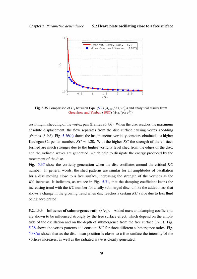
Chapter 5. Parametric dependence 5.2 Heave plate oscillating close to a free surface
0 0.5 1 1.5 2 2.5 3100
101
s/rd
Ca
Present work. Eqn. [5.8]Greenhow and Yanbao (1987)
Fig. 5.35 Comparison of Ca between Eqn. (5.7) (A33/(8/3 ρ r3d)) and analytical results from
Greenhow and Yanbao (1987) (A33/(ρ π r2)).
resulting in shedding of the vortex pair (frames a6, b6). When the disc reaches the maximumabsolute displacement, the flow separates from the disc surface causing vortex shedding(frames a8, b8). Fig. 5.36(c) shows the instantaneous vorticity contours obtained at a higherKeulegan-Carpenter number, KC = 1.20. With the higher KC the strength of the vorticesformed are much stronger due to the higher vorticity level shed from the edges of the disc,and the radiated waves are generated, which help to dissipate the energy produced by themovement of the disc.Fig. 5.37 show the vorticity generation when the disc oscillates around the critical KCnumber. In general words, the shed patterns are similar for all amplitudes of oscillationfor a disc moving close to a free surface, increasing the strength of the vortices as theKC increase. It indicates, as we see in Fig. 5.31, that the damping coefficient keeps theincreasing trend with the KC number for a fully submerged disc, unlike the added mass thatshows a change in the growing trend when disc reaches a certain KC value due to less fluidbeing accelerated.
5.2.4.3.3 Influence of submergence ratio (s/rd). Added mass and damping coefficientsare shown to be influenced strongly by the free surface effect, which depend on the ampli-tude of the oscillation and on the depth of submergence from the free surface (s/rd). Fig.5.38 shows the vortex patterns at a constant KC for three different submergence ratios. Fig.5.38(a) shows that as the disc mean position is closer to a free surface the intensity of thevortices increases, as well as the radiated wave is clearly generated.
79
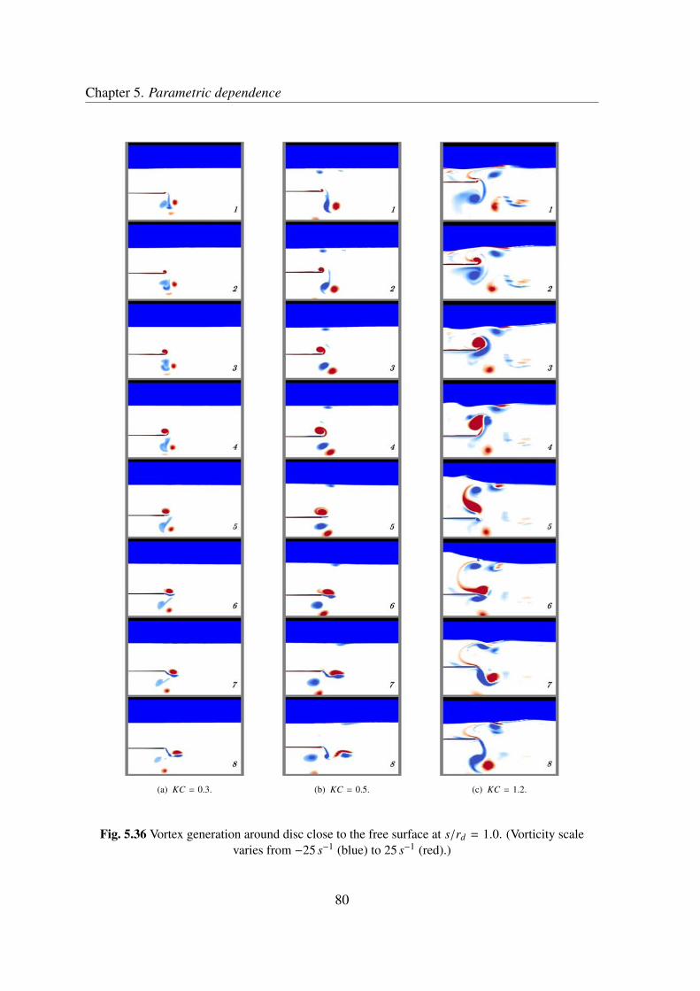
Chapter 5. Parametric dependence
(a) KC = 0.3. (b) KC = 0.5. (c) KC = 1.2.
Fig. 5.36 Vortex generation around disc close to the free surface at s/rd = 1.0. (Vorticity scalevaries from −25 s−1 (blue) to 25 s−1 (red).)
80

Chapter 5. Parametric dependence 5.2 Heave plate oscillating close to a free surface
(a) Vortex generation around the disc atKC/KCcri = 0.80.
(b) Vortex generation around the disc atKC/KCcri = 1.00.
(c) Vortex generation around the disc atKC/KCcri = 1.10.
Fig. 5.37 Vortex generation around the disc at s/rd = 1.0 from the mean free surface. Blue linesindicate negative vorticity (initial condition: Top Dead Centre). Scale varies from −25 s−1(blue) to
25 s−1 (red).
81
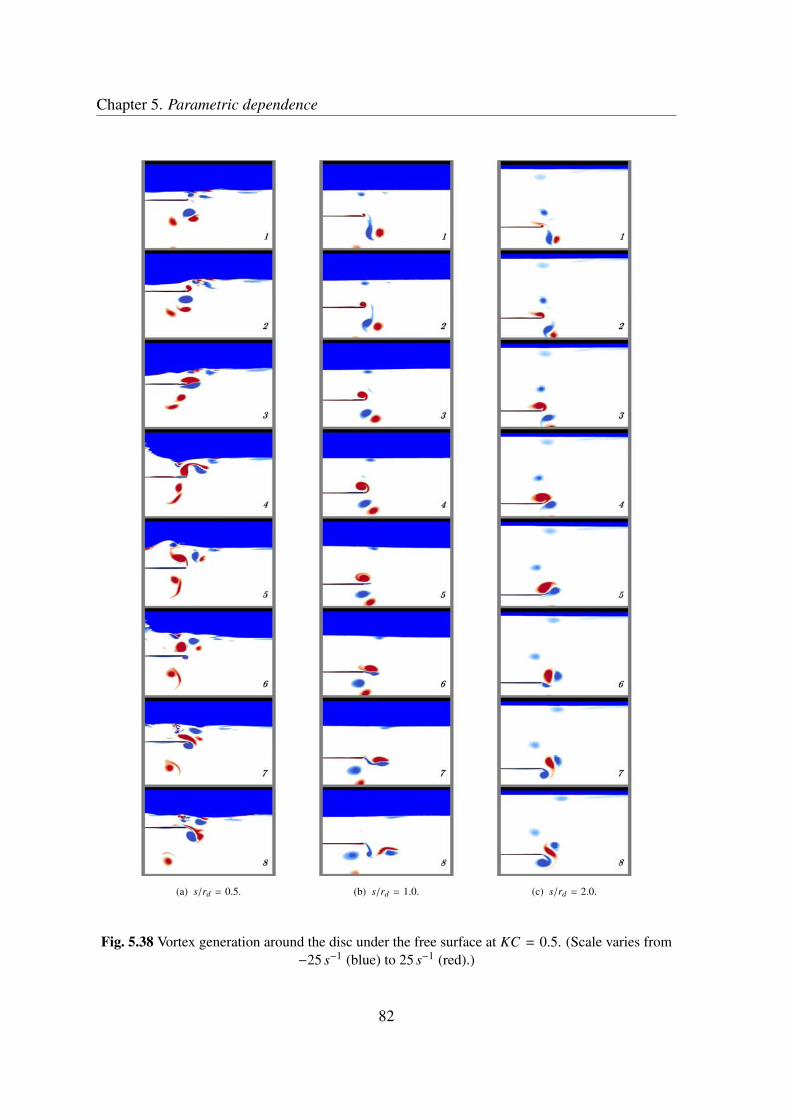
Chapter 5. Parametric dependence
(a) s/rd = 0.5. (b) s/rd = 1.0. (c) s/rd = 2.0.
Fig. 5.38 Vortex generation around the disc under the free surface at KC = 0.5. (Scale varies from−25 s−1 (blue) to 25 s−1 (red).)
82

Chapter 5. Parametric dependence 5.2 Heave plate oscillating close to a free surface
5.2.4.4 Enstrophy and free surface dissipation terms analysis
5.2.4.4.1 KC influence. Unlike the case when the disc oscillates near the seafloor, a discmoving closer to a free surface dissipates energy from the enstrophy term (Eω) and form theradiated waves (E f s).Figures 5.39 to 5.46 show the time history of the enstrophy and free surface dissipationterms for different KC numbers. Fig. 5.40 shows that for a specific submergence ratiothe fluid dissipates more energy as the amplitude of oscillation increases due to the highervorticity shed, and the energy dissipated by the radiated waves also increases (see Fig. 5.42),confirming the linear trends of the damping coefficient.Figs. 5.44 and 5.46 show the dissipation terms at s/rd = 1 for different amplitudes of theoscillation around the critical KC value. From these figures is clearly observed that forlarge KC values, both dissipation terms (Eω and E f s) present a similar quantity of energydissipation, but for smaller KC values the energy dissipation is dominated by the vortexshedding.
15 16 17 18 19 200.03
0.04
0.05
0.06
0.07
0.08
0.09
0.1
0.11
t/T
Eω/ρ
r3 dA
2ω3
KC = 1.20KC = 0.50KC = 0.30
Fig. 5.39 Time history of the enstrophy term from Eqn. (4.20) for an oscillating disc close to thefree surface for different KC values at s/rd = 1.0. Markers correspond to the frames depicted in Fig.
5.36.
83

Chapter 5. Parametric dependence
0 5 10 15 20 250.02
0.03
0.04
0.05
0.06
0.07
0.08
0.09
0.1
0.11
t/T
Eω/ρ
r3 dA
2ω3
KC = 1.20KC = 0.50KC = 0.30
Fig. 5.40 Time history of the enstrophy term from Eqn. (4.20) for an oscillating disc close to thefree surface for different KC values at s/rd = 1.0.
15 16 17 18 19 20−0.05
0
0.05
0.1
0.15
0.2
0.25
0.3
0.35
t/T
Efs/ρ
r3 dA
2ω3
KC = 1.20KC = 0.50KC = 0.30
Fig. 5.41 Time history of the free surface dissipation term from Eqn. (4.21) for an oscillating discclose to the free surface for different KC values at s/rd = 1.0. Markers correspond to the frames
depicted in Fig. 5.36.
5.2.4.4.2 Influence of submergence distance ratio (s/rd). It is also important to ana-lyze the effect that the free surface has on the dissipation terms. Fig. 5.47 and 5.48 showsthe enstrophy and free surface dissipation integral, respectively, for different submergence
84

Chapter 5. Parametric dependence 5.2 Heave plate oscillating close to a free surface
0 5 10 15 20 25−0.2
−0.1
0
0.1
0.2
0.3
0.4
0.5
t/T
Efs/ρ
r3 dA
2ω3
KC = 0.30KC = 0.50KC = 1.20
Fig. 5.42 Time history of the free surface dissipation term from Eqn. (4.21) for an oscillating discclose to the free surface for different KC values at s/rd = 1.0.
8 9 10 11 12 130.005
0.01
0.015
0.02
0.025
0.03
0.035
t/T
Eω[J/s]
KC/KCcri = 0.8
KC/KCcri = 1.0
KC/KCcri = 1.1
Fig. 5.43 Time history of the enstrophy term from Eqn. (4.20) for an oscillating disc close to thefree surface at s/rd = 1.0 around critical KC value. See Figs. 5.31 and 5.37 for h/rd = 1.0.
ratios ‘s’.
85

Chapter 5. Parametric dependence
0 5 10 15 20 250.005
0.01
0.015
0.02
0.025
0.03
0.035
0.04
t/T
Eω[J/s]
KC/KCcri = 0.8
KC/KCcri = 1.0
KC/KCcri = 1.1
Fig. 5.44 Time history of the enstrophy term from Eqn. (4.20) for an oscillating disc close to thefree surface at s/rd = 1.0 around critical KC value.
15 16 17 18 19 200
0.01
0.02
0.03
0.04
0.05
0.06
0.07
0.08
t/T
Efs[J/s]
KC/KCcri = 0.8
KC/KCcri = 1.0
KC/KCcri = 1.1
Fig. 5.45 Time history of the free surface dissipation term from Eqn. (4.21) for an oscillating discclose to the free surface at s/rd = 1.0 around critical KC value. See Figs. 5.31 and 5.37 for
s/rd = 1.0.
86

Chapter 5. Parametric dependence 5.2 Heave plate oscillating close to a free surface
0 5 10 15 20 25−0.02
0
0.02
0.04
0.06
0.08
0.1
t/T
Efs[J/s]
KC/KCcri = 0.8
KC/KCcri = 1.0
KC/KCcri = 1.1
Fig. 5.46 Time history of the free surface dissipation term from Eqn. (4.21) for an oscillating discclose to the free surface at s/rd = 1.0 around critical KC value.
0 5 10 15 20 250
0.1
0.2
0.3
0.4
0.5
0.6
0.7
t/T
Eω/ρ
r3 dA
2ω3
s/rd = 2.0
s/rd = 1.0
s/rd = 0.5
s/rd = 0.4
Fig. 5.47 Time history of the enstrophy term from Eqn. (4.20) for an oscillating disc close to thefree surface for different s/rd values at KC = 0.5.
87
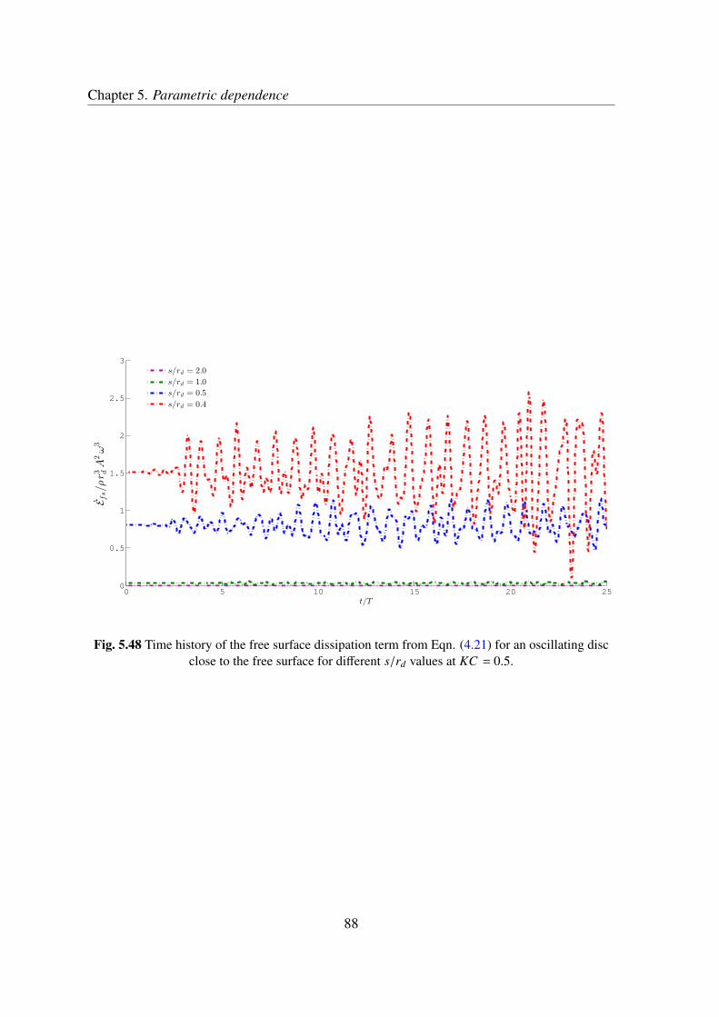
Chapter 5. Parametric dependence
0 5 10 15 20 250
0.5
1
1.5
2
2.5
3
t/T
Efs/ρ
r3 dA
2ω3
s/rd = 2.0
s/rd = 1.0
s/rd = 0.5
s/rd = 0.4
Fig. 5.48 Time history of the free surface dissipation term from Eqn. (4.21) for an oscillating discclose to the free surface for different s/rd values at KC = 0.5.
88

Chapter 5. Parametric dependence 5.2 Heave plate oscillating close to a free surface
5.2.4.4.3 Damping and Enstrophy comparison. The relationship between the dampingcoefficient B33ω obtained through the dissipation terms (Eqn. (4.39)) and the damping co-efficient obtained with the classical forces projection approach (Eqn. (4.47)), are discussedhereinafter. Figs. 5.49 − 5.51 show the comparison of the damping coefficient obtained withboth approaches for three representative cases. The matching is, in general, very good. Thisindicates that the enstrophy and free surface contribution to the dissipation, Eω and EFS ,may be the lead actor in these type of flows.
0 0.2 0.4 0.6 0.8 1 1.2 1.40.2
0.4
0.6
0.8
1
1.2
1.4
1.6
KC
Cb
Total Dissipation. Eω + Efs
Fourier projection
Fig. 5.49 Comparison of hydrodynamic damping coefficient (Cb) with B33 at s/rd = 1.0, obtainedwith Eqn. (4.39) and classical (Sarpkaya and Isaacson, 1981) Fourier projection (Eqn. (4.47)), for
an oscillating heave plate near a free surface.
89

Chapter 5. Parametric dependence
0 0.2 0.4 0.6 0.8 10.4
0.6
0.8
1
1.2
1.4
1.6
1.8
2
2.2
2.4
KC
Cb
Total Dissipation. Eω + Efs
Fourier projection
Fig. 5.50 Comparison of hydrodynamic damping coefficient (Cb) with B33 at s/rd = 0.5, obtainedwith Eqn. (4.39) and classical (Sarpkaya and Isaacson, 1981) Fourier projection (Eqn. (4.47)), for
an oscillating heave plate near a free surface.
0 0.1 0.2 0.3 0.4 0.5 0.6 0.70.8
1
1.2
1.4
1.6
1.8
2
KC
Cb
Total Dissipation. Eω + Efs
Fourier projection
Fig. 5.51 Comparison of hydrodynamic damping coefficient (Cb) with B33 at s/rd = 0.2, obtainedwith Eqn. (4.39) and classical (Sarpkaya and Isaacson, 1981) Fourier projection (Eqn. (4.47)), for
an oscillating heave plate near a free surface.
90

Chapter 5. Parametric dependence 5.3 Analogies Seabed - Free surface
5.3 Analogies between plates oscillating close to free sur-face and seabed
Figs. 5.52 and 5.53 show a comparison of the hydrodynamic coefficients for a disc oscil-lating close to the seabed and the free surface at varying KC numbers. As can be seen, forlarge h/rd or s/rd ratios the coefficients presents similar values at smaller oscillations, anddiffers for higher KC numbers showing that the free surface effects have more influencethan the seafloor. As the disc approaches to the seabed or the free surface (smaller h/rd ors/rd ratios) the coefficients for the free surface case are greater than those when the discoscillates near the seabed.
0 0.25 0.5 0.75 1 1.25 1.5 1.75 2 2.25 2.51
1.1
1.2
1.3
1.4
1.5
1.6
1.7
1.8
1.9
2
Ca
KC
h = 2.0 rd. Seabeds = 2.0 rd. Free Surfaceh = 1.0 rd. Seabeds = 1.0 rd. Free Surfaceh = 0.5 rd. Seabeds = 0.5 rd. Free Surfaceh = 0.4 rd. Seabeds = 0.4 rd. Free Surface
Fig. 5.52 Comparison of added mass coefficient for a disc oscillating close to the seabed and thefree surface using Eqn. (4.46).
91

Chapter 5. Parametric dependence
0 0.25 0.5 0.75 1 1.25 1.5 1.75 2 2.25 2.50
0.2
0.4
0.6
0.8
1
1.2
1.4
1.6
1.8
2
2.2
Cb
KC
h = 2.0 rd. Seabeds = 2.0 rd. Free Surfaceh = 1.0 rd. Seabeds = 1.0 rd. Free Surfaceh = 0.5 rd. Seabeds = 0.5 rd Free Surfaceh = 0.4 rd. Seabeds = 0.4 rd. Free Surface
Fig. 5.53 Comparison of damping coefficient for a disc oscillating close to the seabed and the freesurface using Eqn. (4.47).
92

Chapter 6
Hydrodynamic coefficients of anoscillating semi-submersible column witha heave plate
6.1 General
The motion response, especially heave response, should be minimal for effective and effi-cient working of floating offshore platforms because this motion is primarily responsible forincreasing the downtime as well as causing damage to the risers and moorings systems dueto excessive vertical motion of the platform. In order to reduce heave, damping elementssuch as heave plates are sometimes used.
This section will study the hydrodynamic forces of a semisubmersible column with a heaveplate attached on its bottom.
6.2 Case study description
6.2.1 Experimental investigation
The experiments were conducted in the tow tank at the School of Naval Architecture andOcean Engineering (ETSIN), Technical University of Madrid which has dimensions 100meters long, 3.8 m wide and 2.2 m deep. A sketch of the transversal section (the restrictiveone) of the basin, including the specimen, is presented in Figure 6.1. Regarding eventualbottom effects, the ratio, h/rd, between the distance to the bottom and the disc radius is(2.2−0.775)/0.5 = 2.85. With this ratio and according to the numerical analysis of Garrido-
93
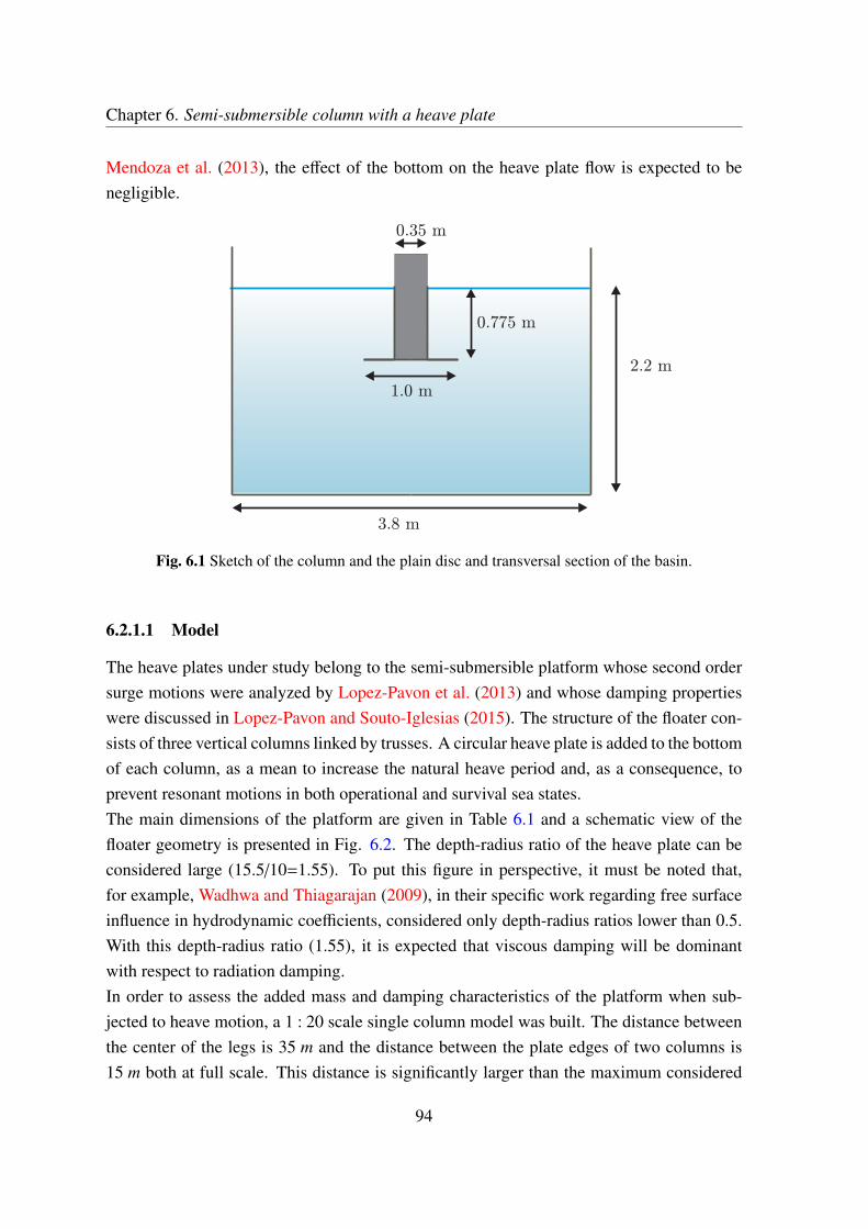
Chapter 6. Semi-submersible column with a heave plate
Mendoza et al. (2013), the effect of the bottom on the heave plate flow is expected to benegligible.
2.2 m
0.775 m
3.8 m
1.0 m
0.35 m
Fig. 6.1 Sketch of the column and the plain disc and transversal section of the basin.
6.2.1.1 Model
The heave plates under study belong to the semi-submersible platform whose second ordersurge motions were analyzed by Lopez-Pavon et al. (2013) and whose damping propertieswere discussed in Lopez-Pavon and Souto-Iglesias (2015). The structure of the floater con-sists of three vertical columns linked by trusses. A circular heave plate is added to the bottomof each column, as a mean to increase the natural heave period and, as a consequence, toprevent resonant motions in both operational and survival sea states.The main dimensions of the platform are given in Table 6.1 and a schematic view of thefloater geometry is presented in Fig. 6.2. The depth-radius ratio of the heave plate can beconsidered large (15.5/10=1.55). To put this figure in perspective, it must be noted that,for example, Wadhwa and Thiagarajan (2009), in their specific work regarding free surfaceinfluence in hydrodynamic coefficients, considered only depth-radius ratios lower than 0.5.With this depth-radius ratio (1.55), it is expected that viscous damping will be dominantwith respect to radiation damping.In order to assess the added mass and damping characteristics of the platform when sub-jected to heave motion, a 1 : 20 scale single column model was built. The distance betweenthe center of the legs is 35 m and the distance between the plate edges of two columns is15 m both at full scale. This distance is significantly larger than the maximum considered
94
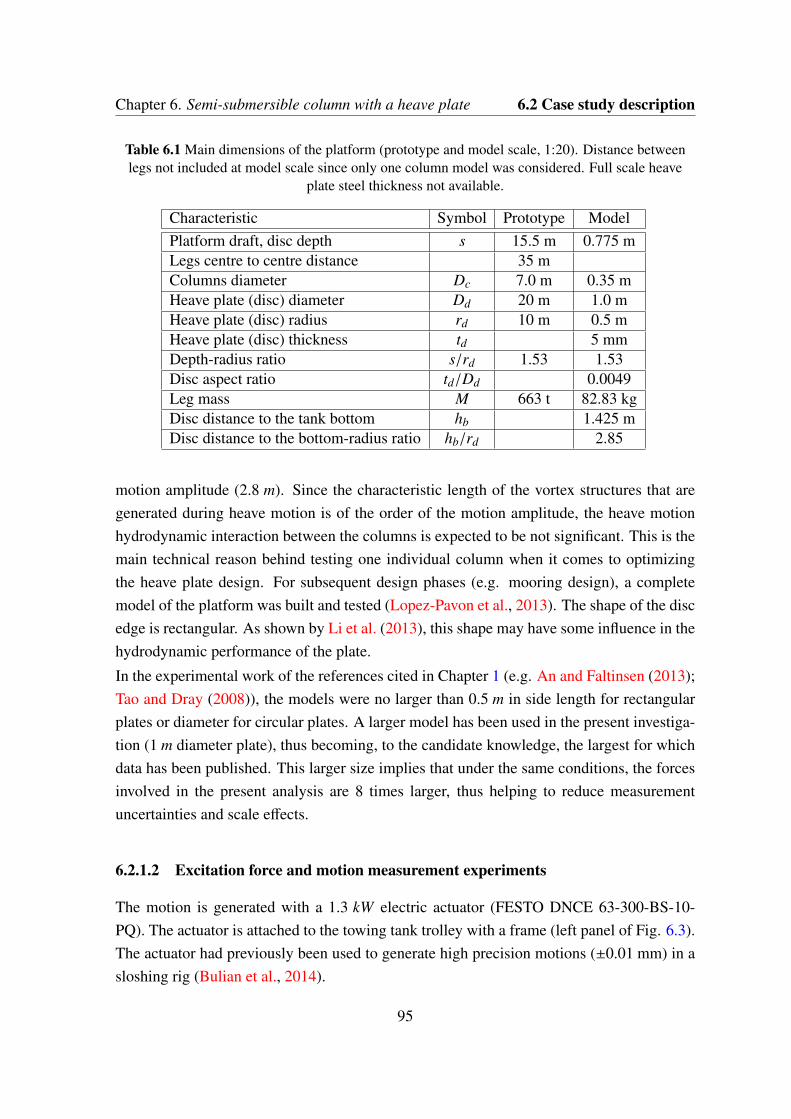
Chapter 6. Semi-submersible column with a heave plate 6.2 Case study description
Table 6.1 Main dimensions of the platform (prototype and model scale, 1:20). Distance betweenlegs not included at model scale since only one column model was considered. Full scale heave
plate steel thickness not available.
Characteristic Symbol Prototype ModelPlatform draft, disc depth s 15.5 m 0.775 mLegs centre to centre distance 35 mColumns diameter Dc 7.0 m 0.35 mHeave plate (disc) diameter Dd 20 m 1.0 mHeave plate (disc) radius rd 10 m 0.5 mHeave plate (disc) thickness td 5 mmDepth-radius ratio s/rd 1.53 1.53Disc aspect ratio td/Dd 0.0049Leg mass M 663 t 82.83 kgDisc distance to the tank bottom hb 1.425 mDisc distance to the bottom-radius ratio hb/rd 2.85
motion amplitude (2.8 m). Since the characteristic length of the vortex structures that aregenerated during heave motion is of the order of the motion amplitude, the heave motionhydrodynamic interaction between the columns is expected to be not significant. This is themain technical reason behind testing one individual column when it comes to optimizingthe heave plate design. For subsequent design phases (e.g. mooring design), a completemodel of the platform was built and tested (Lopez-Pavon et al., 2013). The shape of the discedge is rectangular. As shown by Li et al. (2013), this shape may have some influence in thehydrodynamic performance of the plate.
In the experimental work of the references cited in Chapter 1 (e.g. An and Faltinsen (2013);Tao and Dray (2008)), the models were no larger than 0.5 m in side length for rectangularplates or diameter for circular plates. A larger model has been used in the present investiga-tion (1 m diameter plate), thus becoming, to the candidate knowledge, the largest for whichdata has been published. This larger size implies that under the same conditions, the forcesinvolved in the present analysis are 8 times larger, thus helping to reduce measurementuncertainties and scale effects.
6.2.1.2 Excitation force and motion measurement experiments
The motion is generated with a 1.3 kW electric actuator (FESTO DNCE 63-300-BS-10-PQ). The actuator is attached to the towing tank trolley with a frame (left panel of Fig. 6.3).The actuator had previously been used to generate high precision motions (±0.01 mm) in asloshing rig (Bulian et al., 2014).
95

Chapter 6. Semi-submersible column with a heave plate
Fig. 6.2 Semisubmersible platform case study sketch.
The force signals were measured using a load cell placed between the actuator and the legmodel (center panel of Fig. 6.3). The cell model was Tedea Huntleigh 615-s-type G, with arange of ±200 kg and a precision of 0.02%. This uncertainty is lower than the one associatedto the 24 bits analog-digital converter used.
6.2.1.3 Test matrix
For the model described above, the experiments were mainly divided in four parts:
• Part 1: Tests on solid plain plate at varying depths, oscillation amplitudes and fre-quencies to check the effect of the immersed depth of the plate on the hydrodynamiccoefficients. These tests are thoroughly discussed in Lopez-Pavon and Souto-Iglesias(2015).
96

Chapter 6. Semi-submersible column with a heave plate 6.2 Case study description
Fig. 6.3 (Left) Frame attached to the towing tank trolley, actuator and heave plate. (Center) Loadcell. (Right) Top view of the model.
• Part 2: Tests on plates at different scales, to perform a sensitivity study of scale.
• Part 3: Tests on plates with flaps, to study the influence of the shape of the edge onthe hydrodynamics of the plates.
• Part 4: Tests on fractal heave plate, to investigate the influence of the perforation ratioand hole sizes on the hydrodynamics of the plates.
6.2.1.3.1 Solid heave plate. Vertical oscillations were performed with different ampli-tudes (0.05, 0.1, 0.14 m) and periods (1 to 4 s). For each period, the maximum feasibleamplitude depended on the actuator power, leading to smaller motion amplitudes for thehighest oscillation frequencies. The test matrix is presented in Table 6.2, with β beingthe frequency parameter (Eqn. 4.30), Re the Reynolds number (Eqn. 4.31) and m and psubindexes referring to model and prototype scales respectively. As aforementioned, the ex-periments corresponding to the solid plate are discussed in Lopez-Pavon and Souto-Iglesias(2015). Here the ones corresponding to ω = 2.51 rad/s will be numerically simulated.
The basic geometry to test is formed by a circular Heave Plate and a column of semisub-mersible structure, as show in Figure 6.4:
From the forces measured by the load cell located between the actuator and the leg column,the added mass and damping values are extracted computing the first harmonic of the forceand its phase with respect to the imposed movement.
97
Chapter 6. Semi-submersible column with a heave plate
Table 6.2 Test matrix for a solid heave plate tests.
ω Am T1m KC βm Rem Ap T1p
[rad/s] [m] [s] [m] [s]1.57 0.05 4 0.309 257542 79695 0.985 17.82.09 0.05 3 0.309 342842 106091 0.985 13.32.51 0.05 2.5 0.309 411738 127411 0.985 11.13.14 0.05 2 0.309 515083 159391 0.985 8.94.83 0.05 1.3 0.309 792309 245178 0.985 5.81.57 0.1 4 0.618 257542 159391 1.97 17.82.09 0.1 3 0.618 342842 212183 1.97 13.32.51 0.1 2.5 0.618 411738 254822 1.97 11.13.14 0.1 2 0.618 515083 318782 1.97 8.93.59 0.1 1.8 0.618 588901 364467 1.97 84.83 0.1 1.3 0.618 792309 490355 1.97 5.81.57 0.14 4 0.866 257542 223147 2.758 17.82.09 0.14 3 0.866 342842 297056 2.758 13.32.51 0.14 2.5 0.866 411738 356751 2.758 11.13.14 0.14 2 0.866 515083 446294 2.758 8.9
Fig. 6.4 Geometry of Heave Plate in a column of semisubmersible.
6.2.1.3.2 Scale analysis. It is also important to perform a sensitivity study of scale, toanalyze whether scale effects in the added mass and damping occurs.small scales are fasterthan large ones.
98

Chapter 6. Semi-submersible column with a heave plate 6.2 Case study description
Figure 6.5 shows the different scales of the model and the dimensions of the geometry atdifferent scales are described in Table 6.3.
(a) Model test at scale 1:20. (b) Model test at scale 1:27.6. (c) Model test at scale 1:45.45.
Fig. 6.5 Model of heave plates at different scales.
Table 6.3 Dimensions of the geometry at different scales.
Scale 1. 1:20 Scale 1. 1:27.6 Scale 1. 1:45.45Semisubmersible Column
Diameter [m] 0.354 0.257 0.156Length [m] 1.187 0.860 0.522Thickness [m] 0.003 0.0022 0.0013
Heave PlateDiameter [m] 1.000 0.7246 0.4400Thickness [m] 0.005 0.0036 0.0022
Draft [m]0.775 0.5616 0.341
The experimental parameters for the three scales tests are listed in Table 6.4.
6.2.1.3.3 Heave plate with flaps. Several variations of the basic geometry have beeninvestigated. Heave plates with different flaps are presented in Fig. 6.6 and their dimensionsand IDs are given in Fig. 6.7.Considering that the depth at full-scale is set as 10 m for geometries with flaps, the draftat model scale (1 : 20) will be 0.5 m. Thus, initially it is an objective of these tests and
99

Chapter 6. Semi-submersible column with a heave plate
Table 6.4 Test matrix for the different scales tests.
Prototype Model Scale (1:20) Model Scale (1:27.6) Model Scale (1:45.45)Amplitude Period Frequency Amplitude Period Frequency Amplitude Period Frequency Amplitude Period
A T ω A T ω A T ω A T m>m[s] [rad/s] [m] [s] [rad/s] [m] [s] [rad/s] [m] [s]
1.00 17.89 1.57 0.05 4.00 1.81 0.04 3.46 2.37 0.02 2.651.00 13.42 2.09 0.05 3.00 2.42 0.04 2.60 3.16 0.02 1.991.00 11.18 2.51 0.05 2.50 2.90 0.04 2.16 3.79 0.02 1.661.00 8.94 3.14 0.05 2.00 3.63 0.04 1.73 4.74 0.02 1.331.00 5.81 4.83 0.05 1.30 5.58 0.04 1.13 7.29 0.02 0.862.00 17.89 1.57 0.10 4.00 1.81 0.07 3.46 2.37 0.04 2.652.00 13.42 2.09 0.10 3.00 2.42 0.07 2.60 3.16 0.04 1.992.00 11.18 2.51 0.10 2.50 2.90 0.07 2.16 3.79 0.04 1.662.00 8.94 3.14 0.10 2.00 3.63 0.07 1.73 4.74 0.04 1.332.00 8.05 3.59 0.10 1.80 4.03 0.07 1.56 5.26 0.04 1.192.00 5.81 4.83 0.10 1.30 5.58 0.07 1.13 7.29 0.04 0.862.80 17.89 1.57 0.14 4.00 1.81 0.10 3.46 2.37 0.06 2.652.80 13.42 2.09 0.14 3.00 2.42 0.10 2.60 3.16 0.06 1.992.80 11.18 2.51 0.14 2.50 2.90 0.10 2.16 3.79 0.06 1.662.80 8.94 3.14 0.14 2.00 3.63 0.10 1.73 4.74 0.06 1.33
calculations to find out which heave plate geometry is the most suitable to increase theadded mass (Ca) of the structure and damping. More specifically, different geometries ofthe trailing edge of heave plate will be studied to try to increase the vorticity generationwithout reducing the added mass too much.
6.2.1.3.4 Unconventional design (Fractal heave plate). A novel heave plate based onfractal grid turbulence theory (Cardesa et al., 2012; Cardesa-Dueñas et al., 2011; Nedicet al., 2013) was designed by the candidate. Nedic et al. (2013) found that by increasingthe number of fractal iterations, thus the perimeter, the drag coefficient increases by up to7%. A fractal heave plate was then manufacture and tested experimentally at CEHIPARocean basin. The results were then compared with the solid disc. Figure 6.8 shows thenew fractal heave plate which has been constructed with a porosity of 20% 1 and multipleholes scales, based in the Sierpinski polygon (Bandt and Hung, 2008; Dennis and Schlicker,1995) and more details on its geometric characteristics can be found in Appendix F. Thefractal plate has 5 different holes sizes in order to enhance the hydrodynamic characteristicsof the Solid Plate. It is important to note that the full-scale cost of such kind of designscould be prohibitive compared to a conventional heave plate, but analysing it at model scale(1 : 20)can provide insight into the physics of the problem.The test matrix used in this set of experiments was the same used for the plain heave plate(section 6.2.1.3.1) and was presented in Table 6.2.
1Selection of this porosity was made in order to investigate whether the new heave plate design improvethe hydrodynamic characteristics of the worse porous plate. Total porosity of the fractal heave plate includingthe fractal perimeter is 20%.
100

Chapter 6. Semi-submersible column with a heave plate 6.2 Case study description
(a) Heave plate flap 2.1. (b) Heave plate flap 3.1. (c) Heave plate flap 4.1.
(d) Heave plate flap 4.2. (e) Heave plate flap 4.3.
Fig. 6.6 Model of heave plates with flaps.
6.2.2 CFD calculations.
6.2.2.1 General
In order to investigate the numerical forced heave tests with several amplitudes and differ-ent submergences from the free surface have been carried out. The numerical results arecompared with the experiments conducted in CEHINAV and CEHIPAR model basins, andwith the experimental data by other authors. The aim is to control the natural period (which
101

Chapter 6. Semi-submersible column with a heave plate
Fig. 6.7 Dimensions of the different flaps attached to the heave plate for which experimental datawere available.
depends strongly on the added mass characteristics) and the response amplitude, which de-pends on the damping, so that the floater operates far from its heave natural period or whenthat is not the case, to moderate the motion response.
Figure 6.9 shows the simulation setup and boundary conditions used in all cases in thissection. Dimensions chosen for the numerical tests are based on the model scale 1 : 20.
The no-flux and no-slip velocity boundary conditions are imposed along the oscillatory
102
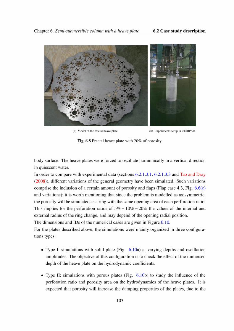
Chapter 6. Semi-submersible column with a heave plate 6.2 Case study description
(a) Model of the fractal heave plate. (b) Experiments setup in CEHIPAR.
Fig. 6.8 Fractal heave plate with 20% of porosity.
body surface. The heave plates were forced to oscillate harmonically in a vertical directionin quiescent water.In order to compare with experimental data (sections 6.2.1.3.1, 6.2.1.3.3 and Tao and Dray(2008)), different variations of the general geometry have been simulated. Such variationscomprise the inclusion of a certain amount of porosity and flaps (Flap case 4.3, Fig. 6.6(e)and variations); it is worth mentioning that since the problem is modelled as axisymmetric,the porosity will be simulated as a ring with the same opening area of each perforation ratio.This implies for the perforation ratios of 5%− 10%− 20% the values of the internal andexternal radius of the ring change, and may depend of the opening radial position.The dimensions and IDs of the numerical cases are given in Figure 6.10.For the plates described above, the simulations were mainly organized in three configura-tions types:
• Type I: simulations with solid plate (Fig. 6.10a) at varying depths and oscillationamplitudes. The objective of this configuration is to check the effect of the immerseddepth of the heave plate on the hydrodynamic coefficients.
• Type II: simulations with porous plates (Fig. 6.10b) to study the influence of theperforation ratio and porosity area on the hydrodynamics of the heave plates. It isexpected that porosity will increase the damping properties of the plates, due to the
103

Chapter 6. Semi-submersible column with a heave plate
Fig. 6.9 Flow domain and boundary conditions.
onset of new vortices. Porosity ranging from 0% (solid) to 20% was used in order tocompare with published experimental data.
• Type III: simulations with Plates with Flaps (Fig. 6.10c-g) to assess to which extentthe hydrodynamic forces are affected by the presence of end plates (wingtips or flaps).
The parameters for the simulations of the three types are listed in Table 6.5.It is relevant mentioning that the range of KC numbers selected (0.12 to 1.4) is typical ofvertical oscillations of deep water offshore structures.All the simulations were conducted with a frequency parameter β of 4 ·105, correspondingto the frequency of oscillation of the cylinder of 0.4Hz. The reason to use one frequencyof oscillation is that as the frequency increases, the value of Ca increases slightly (Li et al.,2013). As a matter of fact, the oscillation frequency has only a slight influence on the added
104

Chapter 6. Semi-submersible column with a heave plate 6.2 Case study description
Fig. 6.10 Dimensions of the different heave plates (units in mm) considered in the CFD simulations.
Table 6.5 Simulation parameters for the heave plates moving closer to the free surface.
Test Submergence [m] A [mm] KC β Re Porosity [%] -s · 105 · 104 ∆R - [mm]
Type I 0.1−0.77 20−230 0.12−1.4 3−5 4.8−56 0 - 0Type II 0.77 50−140 0.31−0.88 4 12−35 5,10,20 -
16,32,65Type III 0.77 50−140 0.31−0.88 4 12−35 10 - 32
mass coefficient of a plate, and the effects of the oscillating frequencies on the dampingcoefficient are small and can be neglected. This observation of the effect of the frequencieson Ca and Cb is consistent with that given by Tao and Dray (2008), Vu et al. (2008) andmore recently by An and Faltinsen (2013).
6.2.2.2 Mesh Generation.
In the same way as in the previous chapter, section 5.1.3, the flow assumption is consideredas axisymmetric, and the meshes for the simulation of the flow induced by the oscillatingvertical disk are generated in a 2D region. A brief description of the mesh characteristics isprovided for each of the configuration types presented in Figure 6.10.
105

Chapter 6. Semi-submersible column with a heave plate
• Type I Configuration. An image of the mesh for this configuration is presented inFigure 6.11. As we can be seen, the grid is fully orthogonal, with progressive variationof the elements sizes.
(a) Typical grid distribution for solid heave plate. (b) Detail of the grid around the solid heave plate.
Fig. 6.11 Mesh generation for Type I configuration.
Here, the heave plate studied is a solid disc, and will serve as basis for comparisonwith the other configurations.
• Type II Configuration. Figure 6.12 shows the configuration mesh for the porositycase studied. Note that the hole region mesh is also refined.
(a) Grid distribution for porous disk. (b) Detail of the grid around the porous disk.
Fig. 6.12 Mesh generation for Type II configuration.
• Type III Configuration. Type III configuration comprises five different heave plates(see Fig. 6.10).
Figure 6.13 shows the meshes of the heave plate with Flap I, located just in the discend.
106

Chapter 6. Semi-submersible column with a heave plate 6.2 Case study description
(a) Grid distribution. (b) Detail of the grid around the Heave Plate.
Fig. 6.13 Mesh generation for Type III configuration, Flap I.
Heave plate meshes with Flap II and III configuration are shown in Figures 6.14 and6.15. The location of the flap is at 150 mm and 75 mm from the edge, respectively, aswe can see in Fig. 6.10.
(a) Grid distribution. (b) Detail of the grid around the Heave Plate.
Fig. 6.14 Mesh generation for Type III configuration, Flap II.
Flap IV (Fig. 6.16) is located radially close to the central column radial position(r/rc = 1.13), at a distance of 300 mm from the edge of the disc.
A variation of Type III configurations is shown in Fig. 6.17, in which the heave plateuse the Flap I and 10% of porosity.
6.2.2.3 Convergence Analysis.
To assess the effects of the spatial and temporal resolutions on the calculated results andcheck numerical convergence, different meshes (Figs. 6.11 to 6.17) and different time-steps,
107
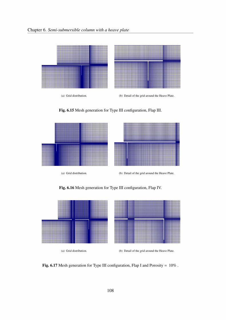
Chapter 6. Semi-submersible column with a heave plate
(a) Grid distribution. (b) Detail of the grid around the Heave Plate.
Fig. 6.15 Mesh generation for Type III configuration, Flap III.
(a) Grid distribution. (b) Detail of the grid around the Heave Plate.
Fig. 6.16 Mesh generation for Type III configuration, Flap IV.
(a) Grid distribution. (b) Detail of the grid around the Heave Plate.
Fig. 6.17 Mesh generation for Type III configuration, Flap I and Porosity = 10% .
108

Chapter 6. Semi-submersible column with a heave plate 6.2 Case study description
keeping the Courant Number (Eqn. 5.1) below 1.0, were investigated.The details of the meshes are listed in Table 6.6. Y+ value, computed as discussed in section5.1.4.2.2, has been included, reading similar values as then.
Table 6.6 Test cases for the influence of the meshes.
Mesh Total number of cellsPoor mesh 100 x 250 25000
Coarser mesh 130 x 260 33300Medium mesh 230 x 300 62400
Finer mesh 290 x 320 88900
The numerical results of force and drag coefficient, obtained from different meshes for KC =0.8796, β = 400000 and ∆t = 1e−4s are presented in Figure 6.18. It has been checked thatCFL < 1 with this ∆t for all cases analyzed.As can be seen in the Figure 6.18(a), the force amplitudes converge quickly. The finest meshseems to present a smoother shape which is related with a force more concentrated in thefrequency of the motion.Figure 6.18(b) indicates that the medium resolution mesh provides a very similar value ofthe drag coefficient when compared to the one obtained with the finest mesh. Therefore, inorder to minimized the computational effort, medium size mesh will be used.In order to determine a suitable time step, a number calculations for different time steps arecarried out for the medium resolution mesh. Figure 6.19(a) shows a comparison betweenforces obtained for different time steps, while Figure 6.19(b) shows that the lowest time stepconsidered may be required for the accurate calculation of the drag coefficient.To take into account the near wall treatment as in Section 5.1.4.2.2 for the case when theheave plate is moving closer to the free surface, the meshes were generated in such a waythat the cells are concentrated near the disk surfaces and stretched out gradually, with aminimum grid spacing of 0.0025 rd around the sharp edges of the disc in radial and verticaldirections, which leads a computational y+ value, based on the cell size of approximately3.7.The simulations reported hereinafter were carried out with a mesh of 230 x 300 cells and atime-step of 1e−4 s.
109

Chapter 6. Semi-submersible column with a heave plate
4 6 8 10 12−1000
−800
−600
−400
−200
0
200
400
600
800
1000
1200
time [s]
Fo
rce
[N
]
25000 cells33300 cells62400 cells88900 cells
(a) Forces obtained for different meshes at KC = 0.8796 and ∆t = 1e−4 s.
25000 cells 33300 cells 62400 cells 88900 cells4
5
6
7
8
9
10
Mesh grid [cells]
CD
(b) Drag coefficient mesh convergence at KC = 0.8796 and ∆t = 1e−4 s using Eqn. (5.2).
Fig. 6.18 Convergence tests in mesh sizes.
110

Chapter 6. Semi-submersible column with a heave plate 6.2 Case study description
4 6 8 10 12−150
−100
−50
0
50
100
150
200
time [s]
Fo
rce
[N
]
∆t=0.002 s ∆t=0.001 s ∆t=0.0005 s ∆t=0.0001 s
(a) Forces obtained for different time step at KC = 0.3142 and 62400 cells.
0.002 0.001 0.0005 0.00017
8
9
10
11
12
13
14
∆T [s]
CD
(b) Drag coefficient time step convergence at KC = 0.3142 and 62400 cells using Eqn.(5.2).
Fig. 6.19 Convergence tests in ∆t.
111

Chapter 6. Semi-submersible column with a heave plate
6.3 Results
6.3.1 General
Forced numerical oscillation analyses have been carried out numerically and compared withexperiments. Heave added mass and damping coefficients have been obtained. The effectsof the different parameters on these coefficients are summarized below.
In order to made non-dimensional the coefficients, theoretical added mass proposed by Sarp-kaya and Isaacson (1981) has been modified to take into account the cylinder + disc config-uration. For a configuration of a cylinder with a disk attached to its base, if the diameter ofthe disk is greater than that of the cylinder, there is only a part of the disk on the cylinderside producing added mass effect due to the presence of the cylinder (see Fig. 6.20). If weassume that the entrained fluid moves as an attached homogeneous mass, by neglecting theinterference between the cylinder and disc, the added mass of a cylinder plus disc may bewritten as, (Tao et al., 2007):
M1a = ρ/12(2D3d +3π D2
d g−π3g3−3π D2c g), (6.1)
where g= 1/π√
D2d −D2
c , Dd and Dc are the heave plate and cylinder diameter, respectively.So, the theoretical added mass can be corrected by accounting for the cylindrical columnvolume.
Fig. 6.20 Added mass of a disc attached to a cylinder. Source: Tao and Cai (2004).
112

Chapter 6. Semi-submersible column with a heave plate 6.3 Results
6.3.2 Solid heave plate: influence of flow parameters KC, β and sub-mergence of the heave plate s/rd
6.3.2.1 General
It is noticed from the measured and calculated data that the added mass and damping coeffi-cients have negligible dependence upon frequency of oscillation at different KC number asshown in Figs. 6.21 and 6.22, which is a consequence of small free-surface wave generation.
0 0.2 0.4 0.6 0.8 11.1
1.2
1.3
1.4
1.5
1.6
1.7
KC
Ca
Tosc,CFD
= 1.999 s
Tosc,CFD
= 2.503 s
Tosc,CFD
= 3.006 s
Tosc,CEHINAV
= 2.497 s
Tosc,CEHINAV
= 3.006 s
Tosc,CEHINAV
= 3.994 s
Tosc,CEHIPAR
= 1.300 s
Tosc,CEHIPAR
= 2.499 s
Tosc,CEHIPAR
= 3.999 s
Fig. 6.21 Added mass with varying frequencies at 1.55rd below mean free surface.
0 0.2 0.4 0.6 0.8 10.3
0.4
0.5
0.6
0.7
0.8
0.9
1
1.1
1.2
1.3
KC
Cb
Tosc,CFD
= 1.999 s
Tosc,CFD
= 2.503 s
Tosc,CFD
= 3.006 s
Tosc,CEHINAV
= 2.497 s
Tosc,CEHINAV
= 3.006 s
Tosc,CEHINAV
= 3.994 s
Tosc,CEHIPAR
= 1.300 s
Tosc,CEHIPAR
= 2.499 s
Tosc,CEHIPAR
= 3.999 s
Fig. 6.22 Damping with varying frequencies at 1.55rd below mean free surface.
It can also be seen in figures above, that there is generally satisfactory agreement betweensimulations and experiments with very slight difference at large KC.
113
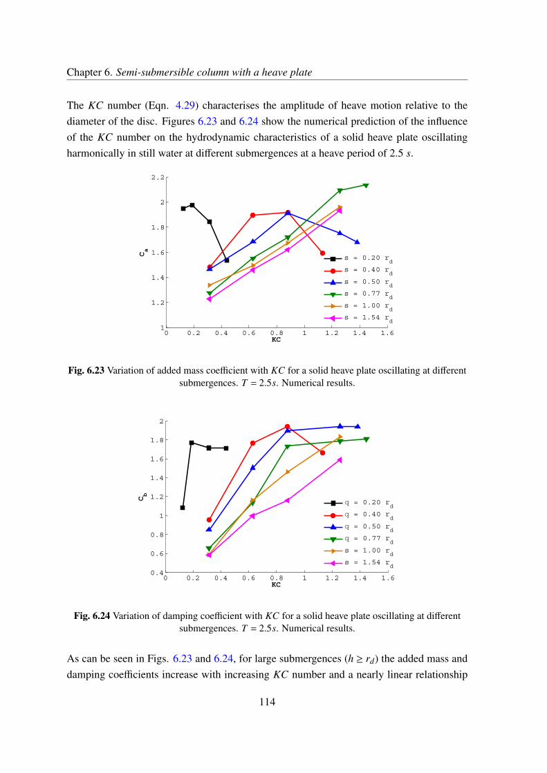
Chapter 6. Semi-submersible column with a heave plate
The KC number (Eqn. 4.29) characterises the amplitude of heave motion relative to thediameter of the disc. Figures 6.23 and 6.24 show the numerical prediction of the influenceof the KC number on the hydrodynamic characteristics of a solid heave plate oscillatingharmonically in still water at different submergences at a heave period of 2.5 s.
0 0.2 0.4 0.6 0.8 1 1.2 1.4 1.61
1.2
1.4
1.6
1.8
2
2.2
Ca
KC
s = 0.20 rd
s = 0.40 rd
s = 0.50 rd
s = 0.77 rd
s = 1.00 rd
s = 1.54 rd
Fig. 6.23 Variation of added mass coefficient with KC for a solid heave plate oscillating at differentsubmergences. T = 2.5s. Numerical results.
0 0.2 0.4 0.6 0.8 1 1.2 1.4 1.60.4
0.6
0.8
1
1.2
1.4
1.6
1.8
2
Cb
KC
= 0.20 rd
= 0.40 rd
= 0.50 rd
= 0.77 rd
s = 1.00 rd
s = 1.54 rd
Fig. 6.24 Variation of damping coefficient with KC for a solid heave plate oscillating at differentsubmergences. T = 2.5s. Numerical results.
As can be seen in Figs. 6.23 and 6.24, for large submergences (h ≥ rd) the added mass anddamping coefficients increase with increasing KC number and a nearly linear relationship
114
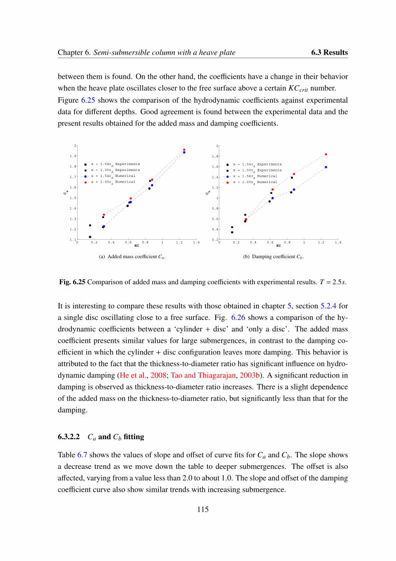
Chapter 6. Semi-submersible column with a heave plate 6.3 Results
between them is found. On the other hand, the coefficients have a change in their behaviorwhen the heave plate oscillates closer to the free surface above a certain KCcrit number.
Figure 6.25 shows the comparison of the hydrodynamic coefficients against experimentaldata for different depths. Good agreement is found between the experimental data and thepresent results obtained for the added mass and damping coefficients.
0 0.2 0.4 0.6 0.8 1 1.2 1.41.1
1.2
1.3
1.4
1.5
1.6
1.7
1.8
1.9
2
KC
Ca
s = 1.54rd Experiments
s = 1.00rd Experiments
s = 1.54rd Numerical
s = 1.00rd Numerical
(a) Added mass coefficient Ca.
0 0.2 0.4 0.6 0.8 1 1.2 1.40.2
0.4
0.6
0.8
1
1.2
1.4
1.6
1.8
2
KC
Cb
s = 1.54rd Experiments
s = 1.00rd Experiments
s = 1.54rd Numerical
s = 1.00rd Numerical
(b) Damping coefficient Cb.
Fig. 6.25 Comparison of added mass and damping coefficients with experimental results. T = 2.5s.
It is interesting to compare these results with those obtained in chapter 5, section 5.2.4 fora single disc oscillating close to a free surface. Fig. 6.26 shows a comparison of the hy-drodynamic coefficients between a ‘cylinder + disc’ and ‘only a disc’. The added masscoefficient presents similar values for large submergences, in contrast to the damping co-efficient in which the cylinder + disc configuration leaves more damping. This behavior isattributed to the fact that the thickness-to-diameter ratio has significant influence on hydro-dynamic damping (He et al., 2008; Tao and Thiagarajan, 2003b). A significant reduction indamping is observed as thickness-to-diameter ratio increases. There is a slight dependenceof the added mass on the thickness-to-diameter ratio, but significantly less than that for thedamping.
6.3.2.2 Ca and Cb fitting
Table 6.7 shows the values of slope and offset of curve fits for Ca and Cb. The slope showsa decrease trend as we move down the table to deeper submergences. The offset is alsoaffected, varying from a value less than 2.0 to about 1.0. The slope and offset of the dampingcoefficient curve also show similar trends with increasing submergence.
115

Chapter 6. Semi-submersible column with a heave plate
0 0.2 0.4 0.6 0.8 1 1.2 1.41
1.1
1.2
1.3
1.4
1.5
1.6
1.7
1.8
1.9
2
KC
Ca
s = 1.54 rd Cylinder + Discs = 2.00 rd Discs = 1.00 rd Cylinder + Discs = 1.00 rd Disc
(a) Added mass coefficient Ca.
0 0.2 0.4 0.6 0.8 1 1.2 1.40.2
0.4
0.6
0.8
1
1.2
1.4
1.6
1.8
2
KC
Cb
s = 1.54 rd Cylinder + Discs = 2.00 rd Discs = 1.00 rd Cylinder + Discs = 1.00 rd Disc
(b) Damping coefficient Cb.
Fig. 6.26 Comparison of added mass and damping coefficients for an oscillating cylinder + disc andonly a disc. Cylinder + disc, td/Dd = 1/200, T = 2.5s. Disc, td/Dd = 1/100, T = 1.0s.
Table 6.7 Slope and offset of curve fits for numerical Ca and Cb.
Submergence Ca Cbs Slope (∂Ca/∂KC) Offset Slope (∂Cb/∂KC) Offset
0.2 rd 0.436 1.949 10.95 1.0830.4 rd 1.320 1.481 2.592 0.9560.5 rd 0.785 1.464 1.856 0.8490.77 rd 0.790 1.276 1.896 0.6541.0 rd 0.665 1.338 1.551 0.5901.54 rd 0.743 1.227 1.039 0.538
Plotting Ca and Cb vs. submergence in Figure 6.27 shows that the slope and offset changequite dramatically for very shallow submergence, but flatten out as we move further awayfrom the free surface. In general for each KC the slope decreases continuously as the heaveplate oscillates at higher submergences s/rd from the free surface. By approximating theslope and offset using an Excel’s tool for a power regression analysis, we found powerformulae that express Ca and Cb in terms of s/rd for each KC ≤ KCcrit value, equations(6.2) and (6.3).
Ca = 0.60(
srd
)−0.25
KC+0.12
srd
+1.0, (6.2)
Cb = 1.25(
srd
)−0.40
KC+0.1
srd
+0.2. (6.3)
116

Chapter 6. Semi-submersible column with a heave plate 6.3 Results
These expressions can be used to evaluate the added mass and damping closer to the freesurface for s/rd ≤ 2 with correlation coefficient R greater than 0.96. Beyond this submer-gence, deep water condition is seen to be the best fit. This condition is the consequence ofthe fact that the added mass approaches its theoretical value expressed by 8/3ρ r3
d for a disc(Korobkin, 2009) and by Eqn. 6.1 for a cylinder+disc (Tao et al., 2007), when KC −→ 0.
0.2 0.4 0.6 0.8 1 1.2 1.4 1.6 1.8 21
1.2
1.4
1.6
1.8
2
2.2
2.4
2.6
Ca
h/rd
R = 0.986
R = 0.992
R = 0.988
KC = 0.31KC = 0.63KC = 0.88
(a) Added Mass Coefficient Ca using Eqn. (6.2).
0.2 0.4 0.6 0.8 1 1.2 1.4 1.6 1.8 20.5
0.7
0.9
1.1
1.3
1.5
1.7
1.9
2.1
2.3
2.5
2.7
2.9
Cb
h/rd
R = 0.988
R = 0.984
R = 0.960
KC = 0.31KC = 0.63KC = 0.88
(b) Damping Coefficient Cb using Eqn. (6.3).
Fig. 6.27 Variation in hydrodynamic coefficients with submergence ‘s/rd’ at varying KC numbers.T = 2.5s. Numerical results.
117

Chapter 6. Semi-submersible column with a heave plate
6.3.2.3 Comparison with other authors
Heave added mass and damping coefficients of solid plates with varying submergences havebeen experimentally examined by Molin et al. (2008).Figure 6.28 shows the experimental and numerical added mass and damping dependenceon KC number. The numerical results show a good agreement with the experimental dataconducted by Molin et al. (2008) for large oscillation period, but there exists an importantdifference in added mass for lower oscillation periods. The weak dependence of Ca on KCfor Molin et al. (2008) experiments is remarkable and challenges our own results and thoseof e.g. Tao and Dray (2008).The differences are probably due to the different geometric characteristics used by the au-thors. Molin performed experiments with smaller (and thinner) disc (diameter 60 cm; thick-ness 1 mm) compared to our disc (diameter 100 cm; thickness 5 mm) and the disc used byTao and Dray (2008) (diameter 40 cm; thickness 8 mm). Smaller damping values obtainedby Tao are attributed to the greater thickness-diameter ratio (td/Dd), parameter that as waspreviously mentioned affect the damping coefficient.
0 0.2 0.4 0.6 0.8 1 1.2 1.4 1.61
1.2
1.4
1.6
1.8
2
2.2
2.4
Ca
KC
Numerical results.Molin et al. (2008). T = 1.2 s.Molin et al. (2008). T = 1.6 s.Tao & Dray (2008). T = 2.0 s.
(a) Added Mass Coefficient Ca.
0 0.2 0.4 0.6 0.8 1 1.2 1.4 1.60.2
0.4
0.6
0.8
1
1.2
1.4
1.6
1.8
2
2.2
2.4
Cb
KC
Numerical resultsMolin et al. (2008). T = 1.2 s.Molin et al. (2008). T = 1.6 s.Tao & Dray (2008). T = 2.0 s.
(b) Damping Coefficient Cb.
Fig. 6.28 Comparison of added mass and damping coefficients for solid heave plate. red line:Present work, s/rd = 0.77 and T = 2.5s. black squares: Molin et al. (2008), s/rd = 0.83 and
T = 1.2s.
6.3.3 Sensitivity study of scale effects
Two set of experiments have been carried out in different facilities in order to verify thereliability of the measurements in the scale analysis. Frequency is made, for the graphs,
118

Chapter 6. Semi-submersible column with a heave plate 6.3 Results
non-dimensional with the theoretical heave resonance frequency of the platform, whosevalue at model scale is:
wr =
√(ρ g S w
M + M1a
), (6.4)
where S w is the water-plane area. The corresponding prototype period (2π/wr) is 17.9 s,which is above common operational first order excitations. The periods to be analyzed havebeen chosen below this value. It is remarkable that without the heave plate, the natural heaveperiod would be 9 s, a value well within typical operational sea states, something that wouldsurely penalize operations by increasing the platform downtime.
Figs. 6.29 and 6.30 show a hydrodynamic coefficient comparison three between differentscales (see Fig. 6.5) of the semi-submersible model. As can be seen the results obtainedexperimentally from models of different scales are quite comparable. This is an encouragingresult, considering that this data needs to be used for prototype design and it seems thatassuming constant values for Ca and Cb is a reasonable extrapolation hypothesis.
6.3.4 Influence of the shape of the heave plate: flaps
This section discusses the influence of the plate edge geometry on the heave response. Sev-eral alternative heave plate edge shapes proposed in Fig. 6.7 have been tested. The presenceof flaps has opposite effects in the heave added mass and damping coefficients, as shownin Figs. 6.31 and 6.32. They increase added mass when compared to the plain plate butsignificantly reduce damping too. This behaviour is due to the influence of the thickness-to-diameter ratio, causing a reduction in the damping coefficient as the td/Dd increases as waspreviously mentioned.
Numerical simulations on five plates with flaps (see Fig. 6.10 and Table 6.5) were alsocarried out and the results were compared with the solid plate, to examine the influence ofvariations on Flap 4.3 on the hydrodynamics. The added mass and damping coefficients ofthese plates obtained numerically, are shown in Figure 6.33. It can be seen that the platewith Flap I yields the greatest added mass but the lowest damping coefficient, while whenthe flap is moved to the center of the heave plate the values of Ca and Cb are quite similarto the hydrodynamic coefficients of the solid plate.
In the behaviour of the heave plate with Flap I and 10% of porosity, the added mass (Fig.6.33(a)) decreases compared to the solid plate and plate with Flap I, due to the flow throughthe porosity. Figure 6.33(b) shows that damping coefficient Cb for the heave plate with ‘FlapI 10% Porosity’ is larger compared to the heave plate with Flap I, but does not improve the
119

Chapter 6. Semi-submersible column with a heave plate
0.8 1 1.2 1.4 1.6 1.8 21.1
1.2
1.3
1.4
1.5
1.6
1.7
1.8
1.9
w/wr
Ca
KC = 0.283cehinav
KC = 0.564cehinav
KC = 0.841cehinav
(a) CEHINAV model basin tests.
0.5 1 1.5 2 2.5 3 3.51.1
1.2
1.3
1.4
1.5
1.6
1.7
1.8
1.9
w/wr
Ca
KC = 0.309cehipar
KC = 0.588cehipar
KC = 0.896cehipar
(b) CEHIPAR model basin tests.
Fig. 6.29 Scale and frequency dependence tests of added mass coefficient. s/rd = 1.55rd. squares:Scale 1 : 20. circles: Scale 1 : 27.6. diamonds: Scale 1 : 45.45.
performance of the solid plate.Fig. 6.34 shows a comparison of the hydrodynamic coefficient obtained experimentally andnumerically, for the heave plate with flap 4.3 configuration. Good agreement between bothresults was found.
120

Chapter 6. Semi-submersible column with a heave plate 6.3 Results
0.8 1 1.2 1.4 1.6 1.8 20.4
0.5
0.6
0.7
0.8
0.9
1
1.1
1.2
1.3
1.4
w/wr
Cb
KC = 0.283cehinav
KC = 0.564cehinav
KC = 0.841cehinav
(a) CEHINAV model basin tests.
0.5 1 1.5 2 2.5 3 3.50.4
0.5
0.6
0.7
0.8
0.9
1
1.1
1.2
1.3
1.4
w/wr
Cb
KC = 0.309
cehipar
KC = 0.588cehipar
KC = 0.896cehipar
(b) CEHIPAR model basin tests.
Fig. 6.30 Scale and frequency dependence tests of damping coefficient. s/rd = 1.55rd. squares:Scale 1 : 20. circles: Scale 1 : 27.6. diamonds: Scale 1 : 45.45.
121
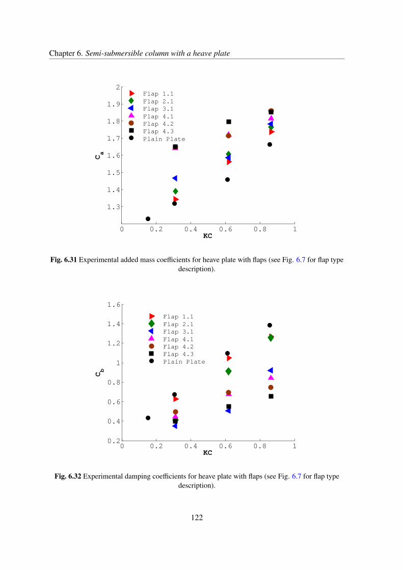
Chapter 6. Semi-submersible column with a heave plate
0 0.2 0.4 0.6 0.8 1
1.3
1.4
1.5
1.6
1.7
1.8
1.9
2
KC
Ca
Flap 1.1Flap 2.1Flap 3.1Flap 4.1Flap 4.2Flap 4.3Plain Plate
Fig. 6.31 Experimental added mass coefficients for heave plate with flaps (see Fig. 6.7 for flap typedescription).
0 0.2 0.4 0.6 0.8 10.2
0.4
0.6
0.8
1
1.2
1.4
1.6
KC
Cb
Flap 1.1Flap 2.1Flap 3.1Flap 4.1Flap 4.2Flap 4.3Plain Plate
Fig. 6.32 Experimental damping coefficients for heave plate with flaps (see Fig. 6.7 for flap typedescription).
122

Chapter 6. Semi-submersible column with a heave plate 6.3 Results
0.2 0.4 0.6 0.8 10.8
1
1.2
1.4
1.6
1.8
2
KC
Ca
Flap I = Flap 4.3Flap II = Flap 4.3bFlap III = Flap 4.3cFlap IV = Flap 4.3dFlap I. Porosity = 10%Plain Plate
(a) Added Mass Coefficient Ca.
0.2 0.4 0.6 0.8 10.2
0.4
0.6
0.8
1
1.2
1.4
1.6
1.8
2
KC
Cb
Flap 4.3Flap 4.3bFlap 4.3cFlap 4.3d
Plain Plate
(b) Damping Coefficient Cb.
Fig. 6.33 Added mass and damping coefficients for heave plate with flaps (Numerical results).
123

Chapter 6. Semi-submersible column with a heave plate
0 0.2 0.4 0.6 0.8 1 1.2 1.4
1.3
1.4
1.5
1.6
1.7
1.8
1.9
2
KC
Ca
Flap 4.3 Exp.Plain Plate Exp.Flap 4.3 Num.Plain Plate Num.
(a) Added Mass Coefficient Ca.
0 0.2 0.4 0.6 0.8 1 1.2 1.40.4
0.6
0.8
1
1.2
1.4
1.6
1.8
2
KC
Cb
Flap 4.3 Exp.Plain Plate Exp.Flap 4.3 Num.Plain Plate Num.
(b) Damping Coefficient Cb.
Fig. 6.34 Comparison of added mass and damping coefficients for heave plate with flaps.
124

Chapter 6. Semi-submersible column with a heave plate 6.3 Results
6.3.5 Influence of the heave plate porosity
6.3.5.1 General
This section investigates the hydrodynamic characteristics of oscillatory porous discs usingnumerical modelling. The sensitivities of the added mass and damping coefficients to bothmotion amplitude and the disc porosity are examined.The heave plates have perforated openings that fit the vertical risers and these openings playan important role in tuning the hydrodynamics of the heave plates. The present study con-cerns simulations on three plates with perforation ratios of 5%, 10% and 10%, respectively.The results are shown in Figs. 6.35 and 6.36, and the hydrodynamic coefficients of the solidplate are also given in those figures for comparison.
0.2 0.4 0.6 0.8 1
0.8
1
1.2
1.4
1.6
1.8
2
KC
Ca
Porosity = 0Porosity = 5%Porosity = 10%Porosity = 20%
Fig. 6.35 Comparison of added mass coefficient for solid and porous plates (Numerical results).T = 2.5s and s = 1.55rd.
Because the fluid can pass through the openings,it is reasonable that the added mass coef-ficient decreases with increasing perforation ratio. As can be seen in Figure 6.35, all discssimulated exhibit a linear increase in added mass coefficient with increasing KC values. Theresults show that the solid disc evidently produces the highest added mass, throughout theKC number range, followed by the 5%, 10% and 20% porous discs, respectively. This isa clear indication that added mass is significantly penalised by the porosity. Natural period(Eqn. (4.32)) will be reduced which may be problematic in case it comes closer to that ofthe extreme or operational waves.
125

Chapter 6. Semi-submersible column with a heave plate
0.2 0.4 0.6 0.8 10.5
0.6
0.7
0.8
0.9
1
1.1
1.2
1.3
1.4
KC
Cb
Porosity = 0Porosity = 5%Porosity = 10%Porosity = 20%
Fig. 6.36 Comparison of damping coefficient for solid and porous plates (Numerical results).T = 2.5s and s = 1.55rd.
Figure 6.36 shows that the discs with 10% of porosity yield the greatest damping. How-ever, the damping coefficient of the heave plate with 5% of porosity are quite similar to thesolid disc values as KC increases. Molin (2001) concluded that the heave damping can beincreased by a factor 4 or 5 by making the heave plate porous with a porosity slightly below20%. It should be noted that his calculation was based on potential flow assumption, andthe analytical solution may yield appropriate values for the damping only if the effect ofseparation through the openings is dominant compared to the effect of separation and vortexshedding due to the disc edge. The increase in Cb due to porosity found in our simulationsis far from his predictions.Figure 6.36 shows that the disc with 20% porosity yields approximately the same value indamping compared to solid disc at KC = 0.314, but clearly under performs all the other discswhen the KC increases, maybe due to increased of the opening area ratio, whereby the flowthrough the perforations reduces the pressure difference between the top and bottom sides ofthe plate and thus the circulation on generation of vorticity at the plate edges, resulting in areduction in heave damping. Figure 6.36 also shows that the optimum porosity, in regards toCb, appears to be between 5% and 10% at low KC numbers. As the KC number increases,such influence appears to diminish. The damping coefficient of these plates with differentperforation ratios are nearly identical to each other at KC > 1.0, which is quite consistentwith the results of Molin (2001) who reported that no extra damping can be gained by
126
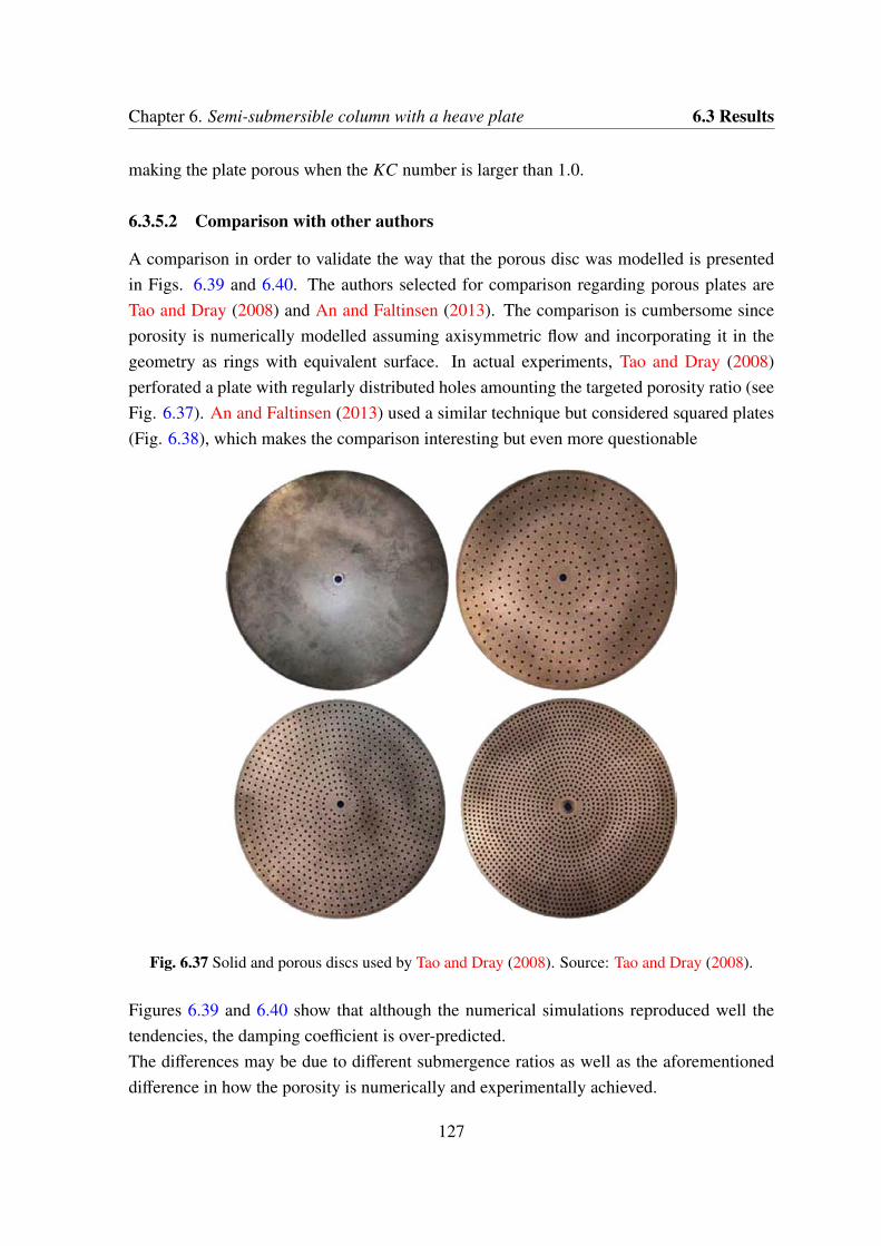
Chapter 6. Semi-submersible column with a heave plate 6.3 Results
making the plate porous when the KC number is larger than 1.0.
6.3.5.2 Comparison with other authors
A comparison in order to validate the way that the porous disc was modelled is presentedin Figs. 6.39 and 6.40. The authors selected for comparison regarding porous plates areTao and Dray (2008) and An and Faltinsen (2013). The comparison is cumbersome sinceporosity is numerically modelled assuming axisymmetric flow and incorporating it in thegeometry as rings with equivalent surface. In actual experiments, Tao and Dray (2008)perforated a plate with regularly distributed holes amounting the targeted porosity ratio (seeFig. 6.37). An and Faltinsen (2013) used a similar technique but considered squared plates(Fig. 6.38), which makes the comparison interesting but even more questionable
Fig. 6.37 Solid and porous discs used by Tao and Dray (2008). Source: Tao and Dray (2008).
Figures 6.39 and 6.40 show that although the numerical simulations reproduced well thetendencies, the damping coefficient is over-predicted.The differences may be due to different submergence ratios as well as the aforementioneddifference in how the porosity is numerically and experimentally achieved.
127

Chapter 6. Semi-submersible column with a heave plate
Fig. 6.38 Porous disc used by An and Faltinsen (2013). Source: An and Faltinsen (2013).
0 0.2 0.4 0.6 0.8 1 1.20.4
0.6
0.8
1
1.2
1.4
1.6
1.8
2
2.2
2.4
KC
Ca
Numerical. Porosity = 0Numerical. Porosity = 5%Numerical. Porosity = 10%Numerical. Porosity = 20%Tao−Dray (2008). Porosity = 0Tao−Dray (2008). Porosity = 5%Tao−Dray (2008). Porosity = 10%Tao−Dray (2008). Porosity = 20%An−Faltinsen (2013). Porosity = 8%An−Faltinsen (2013). Porosity = 16%
Fig. 6.39 Added mass comparison between numerical and experimental results of porous plates.squares: Present work, T = 2.5s and s = 1.8rd. circles: Tao and Dray (2008), T = 2.0s and s = 3.0rd.
diamonds: An and Faltinsen (2013), T = 2.5s and s = 2.85rd.
128

Chapter 6. Semi-submersible column with a heave plate 6.3 Results
0 0.2 0.4 0.6 0.8 1 1.20.2
0.4
0.6
0.8
1
1.2
1.4
1.6
1.8
2
KC
Cb
Numerical. Porosity = 0Numerical. Porosity = 5%Numerical. Porosity = 10%Numerical. Porosity = 20%Tao−Dray (2008). Porosity = 0Tao−Dray (2008). Porosity = 5%Tao−Dray (2008). Porosity = 10%Tao−Dray (2008). Porosity = 20%An−Faltinsen (2013). Porosity = 8%An−Faltinsen (2013). Porosity = 16%
Fig. 6.40 Damping comparison between numerical and experimental results of porous plates.squares: Present work, T = 2.5s and s = 1.8rd. circles: Tao and Dray (2008), T = 2.0s and s = 3.0rd.
diamonds: An and Faltinsen (2013), T = 2.5s and s = 2.85rd.
6.3.6 Fractal plate
6.3.6.1 General
This section discussed the experimental results obtained for the novel fractal heave platedesign introduced in section 6.2.1.3.4. No numerical results are yet available for presentdesign.Figure 6.41 gives the variation of the added mass and damping coefficients at different sub-mergences with KC number. As can be seen in Fig. 6.41(a), when the plate is oscillating todepths greater than 0.5 rd the submergence has little influenced of added mass showing sim-ilar results with a slight variation in slope, although there is a change in the behaviour of Ca
for small submergences. Figure 6.41(b) shows that the Cb increases when the submergencedecreases and there is a nearly linear relationship between Cb and KC.Figure 6.42 shows the comparison of the hydrodynamic coefficients of Fractal Plate andSolid one for submergences s = 1.0rd and s = 0.5rd. As can be seen, the fractal plate showsa similar trend in the behaviour of the coefficients with the solid plate, increasing the valuesof Ca and Cb with the KC number, but under performs the characteristics of the solid plate,maybe due to large porosity used.
129

Chapter 6. Semi-submersible column with a heave plate
0 0.2 0.4 0.6 0.8 1 1.2 1.40.4
0.5
0.6
0.7
0.8
0.9
1
1.1
1.2
1.3Ca
KC
s = 0.200 rd
s = 0.400 rd
s = 0.500 rd
s = 0.770 rd
s = 1.000 rd
s = 1.800 rd
(a) Added Mass Coefficient Ca.
0 0.2 0.4 0.6 0.8 1 1.2 1.40.4
0.6
0.8
1
1.2
1.4
1.6
1.8
Cb
KC
s = 0.200 rd
s = 0.400 rd
s = 0.500 rd
s = 0.770 rd
s = 1.000 rd
s = 1.800 rd
(b) Damping Coefficient Cb.
Fig. 6.41 Variation of hydrodynamic coefficients with KC for a fractal heave plate oscillating atdifferent submergences.
130

Chapter 6. Semi-submersible column with a heave plate 6.3 Results
0 0.2 0.4 0.6 0.8 1 1.2 1.40
0.2
0.4
0.6
0.8
1
1.2
1.4
1.6
1.8
2Ca
KC
s = 1.0 rd Fractal Exp.
s = 1.0 rd Solid Exp.
s = 1.0 rd Solid Num.
s = 0.5 rd Fractal Exp.
s = 0.5 rd Solid Num.
(a) Added Mass Coefficient Ca.
0 0.2 0.4 0.6 0.8 1 1.2 1.40.4
0.6
0.8
1
1.2
1.4
1.6
1.8
2
Cb
KC
s = 1.0 rd Fractal Exp.
s = 1.0 rd Solid Exp.
s = 1.0 rd Solid Num.
s = 0.5 rd Fractal Exp.
s = 0.5 rd Solid Num.
(b) Damping Coefficient Cb.
Fig. 6.42 Comparison of added mass and damping coefficients for solid plate and fractal plate.
131

Chapter 6. Semi-submersible column with a heave plate
6.3.6.2 Comparison between numerical and experimental results by other authors
Molin et al. (2008) also conducted a series of experiments with perforated plates. Figure6.43 shows the comparison of the added mass and damping coefficients for two differentsubmergences ratio. Strong differences are observed for the coefficients between fractalplate and experiments carried by Molin. It should be noticed that our results present thesame behaviour that these found by Molin, and the discrepancies presumably are due to thedifferent value of the diameter and thickness, and mostly due to the fact that the fractal platehas various holes sizes.
0 0.2 0.4 0.6 0.8 1 1.2 1.40
0.2
0.4
0.6
0.8
1
1.2
1.4
Ca
KC
Fractal Exp. s = 0.2 rd
Molin et al. (2008). s = 0.17 rd
Fractal Exp. s = 0.77 rd
Molin et al. (2008). s = 0.83 rd
(a) Added Mass Coefficient Ca.
0 0.2 0.4 0.6 0.8 1 1.2 1.40.2
0.4
0.6
0.8
1
1.2
1.4
1.6
Cb
KC
Fractal Exp. s = 0.2 rd
Molin et al. (2008). s = 0.17 rd
Fractal Exp. s = 0.77 rd
Molin et al. (2008). s = 0.83 rd
(b) Damping Coefficient Cb.
Fig. 6.43 Comparison of added mass and damping coefficients for 20% Porosity heave plate. redline: Present work, T = 2.5s. black line: Molin et al. (2008), T = 1.6s.
Recently, An and Faltinsen (2013) conducted, in a range of submergences, forced harmonicheave motions tests of horizontally perforated rectangular plates. Figure 6.44 shows theexperimental heave added mass and damping coefficients versus KC number, obtained forthe fractal plate (see Fig. 6.8) and compared with the results obtained by An and Faltin-sen. Both set of data correspond to a submergence of approximately s/rd = 0.4, where thepresence of the free surface starts to influence the dynamics. Figure shows that our resultsand these obtained by An and Faltinsen (2013) have a disagreement in value, but presentthe same behaviour for different KC number. Note, that here, the fractal plate has 20% ofporosity, while the rectangular disk (other characteristic for this difference) used by An andFaltinsen has 15.89% of porosity. Even with larger porosity the fractal plate displays largeradded mass and damping performance.Finally, in Fig. 6.45, the fractal plate is compared to Tao and Dray (2008) same porosity(20%) experimental results corresponding to deep water condition. It can be noticed that
132

Chapter 6. Semi-submersible column with a heave plate 6.3 Results
0 0.2 0.4 0.6 0.8 1 1.2 1.40.45
0.5
0.55
0.6
0.65
0.7
0.75
0.8
0.85
0.9
0.95
Ca
KC
Fractal Exp. Porosity = 20%Ann & Faltinsen (2013). Porosity = 15.89%
(a) Added Mass Coefficient Ca.
0 0.2 0.4 0.6 0.8 1 1.2 1.40.4
0.6
0.8
1
1.2
1.4
1.6
1.8
Cb
KC
Fractal Exp. Porosity = 20%Ann & Faltinsen (2013). Porosity = 15.89%
(b) Damping Coefficient Cb.
Fig. 6.44 Comparison of added mass and damping coefficients for porous heave plate. red line:Present work, T = 2.5s and s = 0.4rd. black line: An and Faltinsen (2013), T = 2.0s and s = 0.41rd.
while added mass is similar, the damping values are significantly larger for the fractal platewhen compared with the evenly distributed porosity of Tao and Dray (2008) 20% porosityspecimen. Results of An and Faltinsen (2013) for deep water case, which show a comparableresult when compared between each other.
0 0.5 1 1.5 20.4
0.5
0.6
0.7
0.8
0.9
1
1.1
1.2
1.3
Ca
KC
Fractal Exp. Porosity = 20%Tao−Dray (2008). Porosity = 20%An−Faltinsen (2013). Porosity = 16%
(a) Added Mass Coefficient Ca.
0 0.5 1 1.5 2
0.4
0.5
0.6
0.7
0.8
0.9
1
1.1
1.2
1.3
Cb
KC
Fractal Exp. Porosity = 20%Tao−Dray (2008). Porosity = 20%An−Faltinsen (2013). Porosity = 16%
(b) Damping Coefficient Cb.
Fig. 6.45 Comparison of added mass and damping coefficients for porous heave plate. red line:Present work, T = 2.5s and s = 1.8rd. blue line: An and Faltinsen (2013), T = 2.0s and s = 2.85rd.
black line: Tao and Dray (2008), T = 2.0s and s = 3.0rd.
133

Chapter 7
Conclusions
7.1 Conclusions
The main conclusions of the present work are summarize below:
1. Research on hydrodynamic forces on heave plates attached to oscillating bodies im-mersed in a fluid has been presented.
2. These heave plates are used as motion damping devices in semi-submersible floatingplatforms for offshore wind turbines.
3. The motion model considered is linear. This allows to describe the hydrodynamicforces independently for each frequency.
4. To compute that response forced heave (vertical axis) oscillations are applied at thebody and the forces are measured and their first harmonic is computed.
5. Forces in phase with the motion are defined as the added mass and forces in counter-phase as the damping. The drag coefficient is defined on the basis of this damping.
6. The main parameter defining the flow is the Keulegan-Carpenter number KC. It isdefined as the relation between the amplitude of heave motion and the diameter of theheave plate.
7. Solid and Porous heave plates as well heave plates with flaps have been modellednumerically.
8. Experiments have been conducted with a novel porous heave plate with a fractal pat-tern. Comparisons with data for porous plates by other authors are presented.
135

Chapter 7. Conclusions
9. Numerical open source OpenFOAM code based on the Finite Volume Method (FVM)and Volume of Fluid (VOF) technique used to track the free surface (FS) motion wasused to simulate the axisymmetric viscous flow problem.
10. For the heave plates oscillating closer to the free surface, the added mass and dampingcoefficients increase with the Keulegan-Carpenter number (KC) and with decreasingdistance to free surface. The dependence of the hydrodynamic coefficients is stronglyinfluenced for the free surface, and these coefficients of the solid heave plate werefound to be in good agreement with the experiments.
11. The porosity of the heave plates reduces the added mass for the studied porosity at allKC numbers, but the porous heave plates are found to increase the damping coefficientwith increasing amplitude of oscillation, achieving a maximum damping coefficientfor the heave plate with 10% porosity in all KC range. When the KC number is small,the disk with 20% porosity yields approximately 16% increase in damping comparedto the solid disk, but clearly under performs all the other disks when the KC increases,due to the large opening area ratio.
12. Numerical and experimental results for heave plates with flaps show that keeping theflap near to the end of the disc, increases the added mass when compared to the plainplate but significantly reduce damping too.
13. Simulations conducted on a circular solid disk oscillating at varying elevations fromseabed suggest that as the structure moves closer to seabed the added mass and damp-ing coefficients (Ca and Cb) increases continuously showing slight difference if thebottom is formed with a sandy bed as experiments published by Wadhwa et al. (2010).It can be caused by the cavity formed on the sandy bed when the disk moves close tothe bottom. In the same way as for a heave plates oscillating near the free surface thecoefficients increase with the Keulegan-Carpenter number (KC).
14. The vortex field generated by the oscillating disk appears to have more strength whenthe disk oscillates near the seabed, and this is reflected by the increase of the hydro-dynamic coefficients for the same KC value. The vortex shedding patterns are alteredby increasing KC and by proximity to the seabed.
15. Formulae in order to evaluate the hydrodynamic coefficients closer to free surface andnear the seabed were derived, allowing the calculation of the added mass and dampingwith good agreement for distance ratios h ≤ 2.0 rd.
136
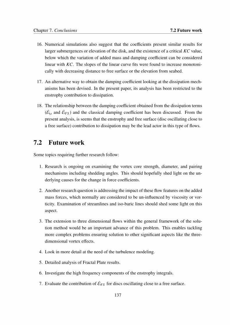
Chapter 7. Conclusions 7.2 Future work
16. Numerical simulations also suggest that the coefficients present similar results forlarger submergences or elevation of the disk, and the existence of a critical KC value,below which the variation of added mass and damping coefficient can be consideredlinear with KC. The slopes of the linear curve fits were found to increase monotoni-cally with decreasing distance to free surface or the elevation from seabed.
17. An alternative way to obtain the damping coefficient looking at the dissipation mech-anisms has been devised. In the present paper, its analysis has been restricted to theenstrophy contribution to dissipation.
18. The relationship between the damping coefficient obtained from the dissipation terms(Eω and EFS ) and the classical damping coefficient has been discussed. From thepresent analysis, is seems that the enstrophy and free surface (disc oscillating close toa free surface) contribution to dissipation may be the lead actor in this type of flows.
7.2 Future work
Some topics requiring further research follow:
1. Research is ongoing on examining the vortex core strength, diameter, and pairingmechanisms including shedding angles. This should hopefully shed light on the un-derlying causes for the change in force coefficients.
2. Another research question is addressing the impact of these flow features on the addedmass forces, which normally are considered to be un-influenced by viscosity or vor-ticity. Examination of streamlines and iso-baric lines should shed some light on thisaspect.
3. The extension to three dimensional flows within the general framework of the solu-tion method would be an important advance of this problem. This enables tacklingmore complex problems ensuring solution to other significant aspects like the three-dimensional vortex effects.
4. Look in more detail at the need of the turbulence modeling.
5. Detailed analysis of Fractal Plate results.
6. Investigate the high frequency components of the enstrophy integrals.
7. Evaluate the contribution of EFS for discs oscillating close to a free surface.
137

Chapter 7. Conclusions
8. Investigate hydrodynamic coefficients for KC numbers above critical KC.
9. It has been found that the ratios between the numerical results and the theoreticalvalues do not tend to one for low KC values, something for which an explanation ismissing, thus deserving further research work.
138
Chapter 8
Thesis Publications
8.1 Refereed papers
• C. Garrido-Mendoza, K.P. Thiagarajan, A. Souto-Iglesias, B. Bouscasse and A. Co-lagrossi. Computation of flow features and hydrodynamic coefficients around heaveplates oscillating near a seabed. Submited for publication.
• Jesús Gómez-Goñi, Carlos A. Garrido-Mendoza, José Luis Cercós, and Leo González.Two phase analysis of sloshing in a rectangular container with Volume of Fluid (VOF)methods. Ocean Engineering, Vol. 73, 208 - 212, 2013.
8.2 Conference papers
• L. Gonzalez, A. Rodriguez, C. Garrido-Mendoza, J. Suarez, and F. Huera-Huarte.CFD simulations on the vortex-induced vibrations of a flexible cylinder with wakeinterference. In ASME, editor, 34th International Conference on Ocean, Offshoreand Arctic Engineering (OMAE). OMAE2015-41128, 2015.
• C. López-Pavón, C. Garrido-Mendoza, and A. Souto-Iglesias. Hydrodynamic forcesand pressure loads on heave plates for semi-submersible floating offshore wind tur-bines: a case study. In ASME, editor, 33rd International Conference on Ocean,Offshore and Arctic Engineering (OMAE). OMAE2014-24163, 2014.
• C. Garrido-Mendoza, K.P. Thiagarajan, A. Souto-Iglesias, B. Bouscasse and A. Co-lagrossi. Numerical investigation of the flow features around heave plates oscillatingclose to a free surface or seabed. In ASME, editor, 33rd International Conference onOcean, Offshore and Arctic Engineering (OMAE). OMAE2014-23818, 2014.
139

Chapter 8. Thesis Publications
• C. Garrido-Mendoza, A. Souto-Iglesias, and K. Thiagarajan. Numerical simulationof hydrodynamics of a circular disk oscillating near a seabed. In ASME, editor,32nd International Conference on Ocean, Offshore and Arctic Engineering (OMAE).OMAE2013-11072, 2013.
140
References
An, S. and Faltinsen, O. M. (2013). An experimental and numerical study of heave addedmass and damping of horizontally submerged and perforated rectangular plates. Journalof Fluids and Structures, 39(0):87 – 101.
Aubault, A., Cermelli, C., and Roddier, D. (2007). Parametric optimization of a semi-submersible platform with heave plates. In ASME 2007 26th International Conferenceon Offshore Mechanics and Arctic Engineering, pages 471–478. American Society ofMechanical Engineers.
Bandt, C. and Hung, N. V. (2008). Fractal n-gons and their Mandelbrot sets. Nonlinearity,21(11):2653–2670.
Batchelor, G. K. (1967). Introduction to Fluid Dynamics. Cambridge University Press, NewYork.
Bearman, P. W., Downie, M. J., Graham, J. M. R., and Obasaju, E. D. (1985). Forces oncylinders in viscous oscillatory flow at low keulegan-carpenter numbers. Journal of FluidMechanics, 154:337–356.
Bernardinis de, B., Graham, J. M. R., and Parker, K. H. (1981). Oscillatory flow arounddisks and through orifices. Journal of Fluid Mechanics, 102:279–299.
Brennen, C. (1982). A review of added mass and fluid inertial forces.
Bulian, G., Botia-Vera, E., and Souto-Iglesias, A. (2014). Experimental sloshing pressureimpacts in ensemble domain: Transient and stationary statistical characteristics. Physicsof Fluids (1994-present), 26(3):–.
Cardesa, J., Nickels, T., and Dawson, J. (2012). 2d piv measurements in the near fieldof grid turbulence using stitched fields from multiple cameras. Experiments in fluids,52(6):1611–1627.
141

Cardesa-Dueñas, J., Nickels, T., and Dawson, J. (2011). Experimental study of homogeni-sation in grid turbulence. In Journal of Physics: Conference Series, volume 318, page032041. IOP Publishing.
Cermelli, C., Morrison, D., Martin, H. C. S., and Guinn, M. (2003). Progression of ultra-deep subsea deployment systems. OTC15147 - Offshore Technology Conference Houston,Texas, U.S.A., (OTC15147).
Chung, J. A. F. (1977). Forces on submerged cylinders oscillating near a free surface.Journal of Hydronautics, 11(3):100–106.
Colagrossi, A., Souto-Iglesias, A., Antuono, M., and Marrone, S. (2013). Smoothed-particle-hydrodynamics modeling of dissipation mechanisms in gravity waves. Phys.Rev. E, 87:023302.
Dennis, K. and Schlicker, S. (1995). Sierpinski N-Gons. Pi Mu Epsilon Journal, 10(2):81–89.
DNV-RP-H103 (April 2010). Modelling and analysis of marine operations. Hovik, Norway.
EWEA (2015). The European offshore wind industry - key trends and statistics 2014. Re-port, EWEA.
Faltinsen, O. M. (1990). Sea loads on ships and offshore structures / O.M. Faltinsen. Cam-bridge University Press.
Ferziger, J. H. and Peric, M. (1999). Computational Methods for Fluid Dynamics. Springer,2nd edition.
Garrido-Mendoza, C., Souto-Iglesias, A., and Thiagarajan, K. (2013). Numerical simu-lation of hydrodynamics of a circular disk oscillating near a seabed. In ASME, edi-tor, 32nd International Conference on Ocean, Offshore and Arctic Engineering (OMAE).OMAE2013-11072.
Garrido-Mendoza, C. A., Thiagarajan, K., Bouscasse, B., Colagrossi, A., and Souto-Iglesias, A. (2014). Numerical Investigation of the Flow Features around Heave PlatesOscillating Close to a Free Surface or Seabed. In ASME, editor, 33rd International Con-ference on Ocean, Offshore and Arctic Engineering (OMAE).
Global Wind Energy Council (2013). Global Wind Report: Annual Market Update 2013.Report, Global Wind Energy Council. http://www.gwec.net/wp-content/uploads/2014/04/GWEC-Global-Wind-Report_9-April-2014.pdf.
142

References
Gomez-Goni, J., Garrido-Mendoza, C. A., Cercos-Pita, J., and Gonzalez, L. (2013). Twophase analysis of sloshing in a rectangular container with volume of fluid (vof) methods.Ocean Engineering, 73(0):208 – 212.
Graham, J. (1980). The forces on sharp-edged cylinders in oscillatory flow at low Keulegan-Carpenter numbers. Journal of Fluid Mechanics, 97:331–346.
Greenhow, M. and Lin, W.-M. (1983). Nonlinear-free surface effects: Experiments andtheory. Technical report, DTIC Document.
Greenhow, M. and Yanbao, L. (1987). Added masses for circular cylinders near or pene-trating fluid boundaries—review, extension and application to water-entry,-exit and slam-ming. Ocean engineering, 14(4):325–348.
Hanson, T., Skaare, B., Yttervik, R., Nielsen, F., and Havmoller, O. (2011). Comparisonof measured and simulated responses at the first full scale floating wind turbine hywind.Technical report, EWEA OFFSHORE.
Haslum, H. A. and Faltinsen, O. M. (1999). Alternative shape of spar platforms for use inhostile areas. Offshore Technology Conference.
He, H., Troesch, A., and Perlin, M. (2008). Hydrodynamics of damping plates at small kcnumbers. In Kreuzer, E., editor, IUTAM Symposium on Fluid-Structure Interaction inOcean Engineering, volume 8 of Iutam Bookseries, pages 93–104. Springer Netherlands.
Herbert, G. J., Iniyan, S., Sreevalsan, E., and Rajapandian, S. (2007). A review of windenergy technologies. Renewable and Sustainable Energy Reviews, 11(6):1117 – 1145.
Heronemus, W. E. (1972). Power from offshore winds. 8th Annual Conference and Exposi-tion on Applications of Marine Technology.
Hirt, C. W. and Nichols, B. D. (1981). Volume of fluid (VOF) method for the dynamics offree boundaries. Journal of Computational Physics, 39(1):201 – 225.
Huse, E. and Utnes, T. (1994). Springing Damping Of Tension Leg Platforms. In 26thAnnual Proceedings of Offshore Technology Conference, number 7446, pages 259–267.The Offshore Technology Conference.
Hvroje, J. (1996). Error Analysis and Estimation for the nite Volume Method with Applica-tion to Fluid Flows. Ph.d. thesis, Imperial College, University of London.
143
IDAE (2011). Plan de energías renovables (PER) 2011−2020. Special report. http://www.idae.es/uploads/documentos/documentos_11227_PER_2011-2020_def_93c624ab.pdf.
Intergovernmental Panel on Climate Change (2012). Renewable Energy Sources and Cli-mate Change Mitigation. Special report. http://www.ipcc.ch/pdf/special-reports/srren/SRREN_Full_Report.pdf.
IREC (2014). Annual Report 2013. Annual report. http://content.irec.cat/annual_report_2013/files/assets/common/downloads/publication.pdf.
Jones, A. and Westwood, A. (2005). Recent progress in offshore renewable energy technol-ogy development. Power engineering society general meeting, 2:2017–2022.
Keulegan, G. H. and Carpenter, L. H. (1958). Forces on cylinders and plates in an oscillatingfluid. Journal of Research of the National Bureau of Standards, 60(5):423–440.
Korobkin, A. (2009). Added Masses of Three-Dimensional Bodies in Infinite Fluid. InAdded Masses of Ship Structures, volume 88 of Fluid Mechanics and Its Applications,pages 81–102. Springer Netherlands.
Lake, M., He, H., Troesch, A. W., Perlin, M., and Thiagarajan, K. P. (2000). HydrodynamicCoefficient Estimation for TLP and Spar Structures. Journal of Offshore Mechanics andArctic Engineering, 122(2):118–124.
Lamb, H. (1945). Hydrodynamics. Dover Books on Physics. Dover publications.
Larsson, L. and Baba, E. (1996). Ship resistance and flow computations. Advances inmarine Hydrodynamics, pages 1–75.
LeVeque, R. J. (2002). Finite volume methods for hyperbolic problems, volume 31. Cam-bridge university press.
Li, J., Liu, S., Zhao, M., and Teng, B. (2013). Experimental investigation of the hydro-dynamic characteristics of heave plates using forced oscillation. Ocean Engineering,66(0):82 – 91.
LLC., M. I. C. (2012). Floating offshore wind foundations: Industry consortia and projectsin the united states, europe and japan. Technical report, Maine International ConsultingLLC.
144

References
Lopez-Pavon, C. and Souto-Iglesias, A. (2015). Hydrodynamic Coefficients and Pressureloads on Heave Plates for Semi-Submersible Floating Offshore Wind Turbines: a Com-parative Analysis Using Large Scale Models. Renewable Energy (in press).
Lopez-Pavon, C., Watai, R. A., Ruggeri, F., Simos, A. N., and Souto-Iglesias, A. (2013).Influence of wave induced second-order forces in semi-submersible FOWT mooring de-sign. In ASME 32nd International Conference on Ocean, Offshore and Arctic Engineer-ing, OMAE2013.
Marsh, G. (2014). Greater role for composites in wind energy. Reinforced Plastics, 58(1):20– 24.
Molin, B. (2001). On the Added Mass and Damping of Periodic Arrays of Fully or PartiallyPorous Disks. Journal of Fluids and Structures, 15(2):275 – 290.
Molin, B. (2011). Hydrodynamic modeling of perforated structures. Applied Ocean Re-search, 33(1):1 – 11.
Molin, B., Guérin, P., Martigny, D., and Weber, P. (1999). Etude théorique et expérimentaledes efforts hydrodynamiques sur une embase plane à l’approche du fond marin. Actes7èmes Journées de l’Hydrodynamique, pages 291–304.
Molin, B. and Korobkin, A. (2001). Water entry of a perforated wedge. In Proceedings ofthe 16th International Workshop on Water Waves and Floating Bodies.
Molin, B. and Nielsen, F. (2004). Heave added mass and damping of a perforated disk belowthe free surface. In Proceedings of the 19th International Workshop on Water Waves andFloating Bodies.
Molin, B., Remy, F., and Ripol, T. (2008). Experimental study of the heave added mass anddamping of solid and perforated disks close to the free surface. In International Congressof International Maritime Association of the Mediterranean, Varna, Bulgarie.
Morrison, D. and Cermelli, C. (2003). Deployment of subsea equipment in ultradeep water.ASME Conference Proceedings, 2003(36819):341–349.
Musial, W., Butterfield, S., and Boone, A. (2004). Feasibility of floating platform systemsfor wind turbines. In 23rd ASME Wind Energy Symposium, Reno, NV.
Nallayarasu, S. and Bairathi, K. (2014). Hydrodynamic response of spar hulls with heavedamping plate using simplified approach. Ships and Offshore Structures.
145
Nedic, J., Ganapathisubramani, B., and Vassilicos, J. (2013). Drag and near wake charac-teristics of flat plates normal to the flow with fractal edge geometries. Fluid DynamicsResearch, 45(6):061406.
Nicholls-Lee, R., Micklethwaite, W., Walker, R., and Argall, R. (2014). Novel, Practicaland Effective: a Feasibility Study for a Low Motion, Floating Wind Turbine Platform. InAsme, editor, 33rd International Conference on Ocean, Offshore and Arctic Engineering(OMAE).
Nielsen, F., Hanson, T., and Skaare, B. (2006). Integrated dynamic analysis of floatingoffshore wind turbines. In Proceedings of the 25th International Conference on OffshoreMechanics and Arctic Engineering (OMAE). ASME.
OpenCFD, L. (2013). OpenFOAM - User Guide. http://foam.sourceforge.net/docs/Guides-a4/UserGuide.pdf, version 2.2.1 edition.
OpenCFD Ltd. (2013). OpenFOAM - Programmer’s Guide.http://foam.sourceforge.net/docs/Guides-a4/ProgrammersGuide.pdf, version 2.2.1edition.
PANER (2010). Plan de acción nacional de energías renovables de españa 2011−2020. Spe-cial report. http://www.minetur.gob.es/energia/desarrollo/EnergiaRenovable/Documents/20100630_PANER_Espanaversion_final.pdf.
Philip, N. T., Nallayarasu, S., and Bhattacharyya, S. (2012). Damping characteristics ofheave plates attached to spar hull. In ASME 2012 31st International Conference onOcean, Offshore and Arctic Engineering, pages 249–260. American Society of Mechani-cal Engineers.
Pistani, F. and Thiagarajan, K. (2006). Assessment of dynamic factors for subsea deploye-ment from crane vessels. Technical Report No. R2D3-UWA-05-561.
Prislin, I., Blevins, R., and Halkyard, J. (1998). Viscous damping and added-mass of solidsquare plates. In Proceedings of the 17th International Conference on Offshore Mechan-ics and Arctic Engineering (OMAE). ASME.
Real decreto ley 1/2012 (2012). Boletín Oficial del Estado BOE. Special report. http://www.boe.es/boe/dias/2012/01/28/pdfs/BOE-A-2012-1310.pdf.
REE (2014). The Spanish Electricity System. Preliminary report. http://www.ree.es/sites/default/files/downloadable/preliminary_report_2014.pdf.
146

References
Roddier, D., Cermelli, C., Aubault, A., and Weinstein, A. (2010). Windfloat: A floatingfoundation for offshore wind turbines. Journal of Renewable and Sustainable Energy,2(3):–.
Roddier, D., Cermelli, C., and Weinstein, A. (2009). Windfloat: A floating foundation foroffshore wind turbines—part i: Design basis and qualification process. In Proceedings ofthe 28th International Conference on Ocean, Offshore and Arctic Engineering (OMAE),volume Volume 4: Ocean Engineering; Ocean Renewable Energy; Ocean Space Utiliza-tion, Parts A and B, pages 845–853. ASME: OMAE2009-79229.
Roveri, F., Oliveira, M. D., and Moretti, M. (1996). Installation of a production manifold in2000 ft water depth offshore brazil. OTC8237 - Offshore Technology Conference Houston,Texas, U.S.A., (OTC8237).
Salim, S. M. and Cheah, S. C. (2009). Wall y + Strategy for Dealing with Wall-boundedTurbulent Flows. In Proceedings of the International MultiConference of Engineers andComputer Scientists, volume Vol. II. IMECS.
Sarpkaya, T. and Isaacson, M. (1981). Mechanics of wave forces on offshore structures.New York: van Nostrand Reinhold.
Sudhakar, S. and Nallayarasu, S. (2011). Influence of heave plate on hydrodynamic re-sponse of SPAR. In ASME 30th International Conference on Ocean, Offshore and ArcticEngineering, OMAE2011.
Sumer, B. and Fredsøe, J. (1997). Hydrodynamics around cylindrical structures. WorldScientific Publ.
Tao, L. and Cai, S. (2004). Heave motion suppression of a spar with a heave plate. OceanEngineering, 31(5–6):669 – 692.
Tao, L., Cheng, L., and Thiagarajan, K. (1999). Numerical estimation of hydrodynamicheave damping of a vertical cylinder with appendages. In Proceedings of the Ninth Inter-national Offshore and Polar Engineering Conference, volume Vol III, 490-495.
Tao, L. and Dray, D. (2008). Hydrodynamic performance of solid and porous heave plates.Ocean Engineering, 35(10):1006 – 1014.
Tao, L., Molin, B., Scolan, Y.-M., and Thiagarajan, K. (2007). Spacing effects on hy-drodynamics of heave plates on offshore structures. Journal of Fluids and Structures,23(8):1119 – 1136.
147

Tao, L. and Thiagarajan, K. (2000). The influence of edge sharpness on the heave dampingforces experienced by a tlp column. In Tenth International Offshore and Polar Engineer-ing conference, volume Volume 1, pages 277–282. ISOPE.
Tao, L. and Thiagarajan, K. (2003a). Low KC flow regimes of oscillating sharp edges I.Vortex shedding observation. Applied Ocean Research, 25(1):21 – 35.
Tao, L. and Thiagarajan, K. (2003b). Low KC flow regimes of oscillating sharp edges. II.Hydrodynamic forces. Applied Ocean Research, 25(2):53 – 62.
Tao, L., Thiagarajan, K., and Cheng, L. (2000). On the parametric dependence of springingdamping of tlp and spar columns. Applied Ocean Research, 22(5):281 – 294.
Thiagarajan, K. (1993). Hydrodynamics of oscillating cylinder and disks at low Keulegan-Carpenter numbers. Ph.d. thesis, Department of Naval Architecture and Marine Engi-neering, The University of Michigan.
Thiagarajan, K. P. and Troesch, A. W. (1998). Effects of appendages and small currents onthe hydrodynamic heave damping of tlp columns. Journal of Offshore Mechanics andArctic Engineering, 120(1):37–42.
Thurston, K. W., Swanson, R. C., and Kopp, F. (2011). Statistical characterization of slack-ing and snap loading during offshore lifting and lowering in a wave environment. ASMEConference Proceedings, 2011(44335):269–277.
Ubbink, O. (1997). Numerical Prediction of Two Fluid Systems with Sharp Interfaces. Ph.d.thesis, Imperial College, University of London.
Utnes, T., Eidsvik, K. J., and Moe, G. (1995). Dynamic separation over bluff bodies predic-tions based upon reynolds equations. Journal of Hydraulic Research, 33(2):219–242.
Versteeg, H. and Malalasekera, W. (1995). An introduction to Computational FluidDynam-ics,the Finite Volume Method. Harlow: Longman Scientific and Technical.
Vinje, T. (2001). Fluid flow through perforated structures. Technical report, MarinConsultReport.
Viselli, A. M., Goupee, A. J., and Dagher, H. J. (2014). Model Test of a 1:8 Scale Float-ing Wind Turbine Offshore in the Gulf of Maine. In Asme, editor, 33rd InternationalConference on Ocean, Offshore and Arctic Engineering (OMAE).
148

References
Vu, K. H., Chenu, B., and Thiagarajan, K. P. (2008). Hydrodynamic damping due to porousplates. In Proc. World Scientific and Engineering Academy and Society, Greece.
Wadhwa, H., Krishnamoorthy, B., and Thiagarajan, K. P. (2010). Variation of Heave AddedMass and Damping Near Seabed. In ASME 29th International Conference on OffshoreMechanics and Arctic Engineering, OMAE.
Wadhwa, H. and Thiagarajan, K. P. (2009). Experimental Assessment of HydrodynamicCoefficients of Disks Oscillating Near a Free Surface. In ASME 28th International Con-ference on Offshore Mechanics and Arctic Engineering, OMAE.
149


Appendices
151

Appendix A
Energy Eqn. with control Volume.
Considering a generic control volume Vc(t), the transport theorem for a generic fluid quan-tity f reads:
DDt
∫Vc(t)
(ρ f )dV =∫
Vc(t)ρ
D fDt
dV +∫∂Vc(t)
(vb−u) · n(ρ f )dS (A.1)
Substituting f = (u2/2−G) in Eqn. (A.1) yields:
DDt
∫Vc(t)
(u2/2−G)ρdV =∫
Vc(t)ρ
D(u2/2−G)Dt
dV +∫∂Vc(t)
ρ (u2/2−G)(vb−u) · ndS
(A.2)Using Eqn. (4.9) it can be rewritten as:
EM =
∫∂Vc(t)
Tu · ndS −∫
Vc(t)T : DdV +
∫∂Vc(t)
ρ(u2/2 + gz )(vb−u) · ndS (A.3)
The surface of the control volume ∂Vc can be divided as ∂Vc = ∂ΩF ∪ ∂ΩB ∪∂ΩC ∪∂ΩG
where ∂ΩF is the free surface, ∂ΩB the surface of the moving solid body, ∂ΩG the seabedand ∂ΩC a control surface which closes the domain (Fig. 4.2). Therefore, the first right hand
153
Appendix B. Energy Eqn. with control Volume.
side term from Eqn. (A.3) can be decoupled as:∫∂Vc(t)
Tu · ndS =
∫∂ΩF (t)
(Tn) ·udS +∫∂ΩG(t)
(Tn) ·udS +∫∂ΩB(t)
(Tn) ·udS +∫∂ΩC(t)
(Tn) ·udS +
= Pbody/ f luid +
∫∂ΩC(t)
(Tn) ·udS .
(A.4)
The first two surface integrals are null since the stress is zero on ∂ΩF and velocity is zero inthe seabed. The last term of Eqn. (A.3) becomes:∫
∂ΩVc(t)ρ (u2/2 + gz ) (vb−u) · n dS =
∫∂ΩB(t)
ρ (u2/2 + gz ) (vB−u) · ndS +∫∂ΩG(t)
ρ (u2/2 + gz ) (vG −u) · ndS +∫∂ΩF (t)
ρ (u2/2 + gz ) (vF −u) · ndS +∫∂ΩC(t)
ρ (u2/2 + gz ) (vC −u) · ndS ,
(A.5)
where the three first integrals of the right-hand side are null since v = u, and eqn. (A.3) thusbecomes:
EM = Pbody/ f luid +
∫Vc(t)T : DdV +
∫∂ΩC(t)
[ρ (vC −u)(u2/2 + gz ) + Tu
]· ndS . (A.6)
The second term on the right hand side is the fluid dissipated power ED, which can bedecomposed as in section B using Eqn. (B.1):
ED = Ewall+ EFS + Eω −2µ∫∂ΩC(t)
(∇uu) · ndS . (A.7)
154

Appendix B. Energy Eqn. with control Volume.
Using the constitutive equation (4.3), Eqn. (A.6) can be reshaped as:
EM = PPressurebody/ f luid + PViscous
body/ f luid + PPressureControl + PViscous
Control +∫∂ΩC(t)
ρ (u2/2 + gz )(vC −u) · ndS +
Eω + EFS ,
(A.8)
where the power terms Pcontrol are defined as:
PPressureControl := −
∫∂ΩC(t)
p n · udS , PViscousControl := −µ
∫∂ΩC(t)
(ω × n) · udS (A.9)
155


Appendix B
Decomposition of the dissipation term.
Adding and substracting enstrophy, Eqn. (4.15) can be written as:
ED = −2µ∫Ω
D : DdV = −2µ∫∂Ω
(∇uu) · ndS − µ∫Ω
ω2 dV . (B.1)
Defining
Eω := −µ∫Ω
ω2 dV ,
EFS := −2µ∫∂ΩF
(∇uu) · ndS ,
Ewall := −2µ∫∂ΩB
(∇uuB) · ndS ,
(B.2)
the viscous dissipation power can be decomposed as:
ED := Ewall+ EFS + Eω . (B.3)
Rearranging Eqn. (B.3) and Eqn. (4.16) we get:
EM =(Pext + Ewall
)+ EFS + Eω . (B.4)
The sum (Pext + Ewall) can be rewritten as:
Pext + Ewall =
∫∂ΩB
Tn ·uB dS − 2µ∫∂ΩB
(∇uuB) · ndS , (B.5)
and using the constitutive Eqn. (4.3) we get:
Pext + Ewall =
∫∂ΩB
−puB · ndS − µ∫∂ΩB
(ω × uB) · ndS . (B.6)
157
Appendix C. Decomposition of the dissipation term.
Defining
PPressurebody/ f luid := −
∫∂ΩB
puB · ndS , PViscousbody/ f luid := −µ
∫∂ΩB
(ω × n) · uB dS (B.7)
the Eqn. (B.4) can be finally expressed as:
EM = PPressurebody/ f luid + PViscous
body/ f luid + EFS + Eω . (B.8)
158

Appendix C. Decomposition of the dissipation term. B.1 Enstrophy integral
B.1 Enstrophy volume integral in OpenFOAM
/*---------------------------------------------------------------------------*\License This file is based on the OpenFOAM provided one enstrophy.C
Copyright (C) 2015 Carlos Ariel Garrido-Mendoza <[email protected]>
This file is free software: you can redistribute it and/or modify it under the terms of the GNU General Public License as published by the Free Software Foundation, either version 3 of the License, or (at your option) any later version.
This file is distributed in the hope that it will be useful, but WITHOUT ANY WARRANTY; without even the implied warranty of MERCHANTABILITY or FITNESS FOR A PARTICULAR PURPOSE. See the GNU General Public License for more details.
You should have received a copy of the GNU General Public License along with this file. If not, see <http://www.gnu.org/licenses/>.
Application Enstrophy Integral
Description Calculates and writes the Enstrophy of the velocity field U.
The -noWrite option just outputs the max/min values without writing the field.
\*---------------------------------------------------------------------------*/
#include "calc.H"#include "fvc.H"
// * * * * * * * * * * * * * * * * * * * * * * * * * * * * * * * * * * * * * //
void Foam::calc(const argList& args, const Time& runTime, const fvMesh& mesh)
bool writeResults = !args.optionFound("noWrite");
IOobject Uheader(
"U",runTime.timeName(),mesh,IOobject::MUST_READ
);
if (Uheader.headerOk())
Info<< " Reading U" << endl;volVectorField U(Uheader, mesh);
Info<< " Calculating enstrophy" << endl;volScalarField Int_enstrophy(
159
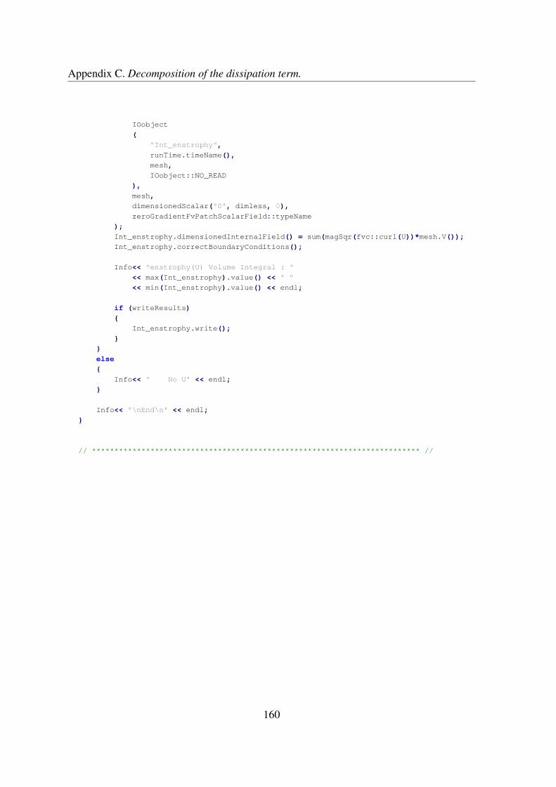
Appendix C. Decomposition of the dissipation term.
IOobject(
"Int_enstrophy",runTime.timeName(),mesh,IOobject::NO_READ
),mesh,dimensionedScalar("0", dimless, 0),zeroGradientFvPatchScalarField::typeName
);Int_enstrophy.dimensionedInternalField() = sum(magSqr(fvc::curl(U))*mesh.V());Int_enstrophy.correctBoundaryConditions();
Info<< "enstrophy(U) Volume Integral : "<< max(Int_enstrophy).value() << " "<< min(Int_enstrophy).value() << endl;
if (writeResults)
Int_enstrophy.write();
else
Info<< " No U" << endl;
Info<< "\nEnd\n" << endl;
// ************************************************************************* //
160

Appendix C. Decomposition of the dissipation term. B.2 Free surface dissipation integral
B.2 Free surface dissipation surface integral in OpenFOAM
/*---------------------------------------------------------------------------*\License This file is based in the OpenFOAM provided one enstrophy.C
Copyright (C) 2015 Carlos Ariel Garrido-Mendoza <[email protected]>
This file is free software: you can redistribute it and/or modify it under the terms of the GNU General Public License as published by the Free Software Foundation, either version 3 of the License, or (at your option) any later version.
This file is distributed in the hope that it will be useful, but WITHOUT ANY WARRANTY; without even the implied warranty of MERCHANTABILITY or FITNESS FOR A PARTICULAR PURPOSE. See the GNU General Public License for more details.
You should have received a copy of the GNU General Public License along with this file. If not, see <http://www.gnu.org/licenses/>.
Application Free Surface dissipation Integral
Description Calculates and writes the dissipation of the Free Surface.
The -noWrite option just outputs the max/min values without writing the field.
\*---------------------------------------------------------------------------*/
#include "calc.H"#include "fvc.H"
// * * * * * * * * * * * * * * * * * * * * * * * * * * * * * * * * * * * * * //
void Foam::calc(const argList& args, const Time& runTime, const fvMesh& mesh)
bool writeResults = !args.optionFound("noWrite");
IOobject Uheader(
"U",runTime.timeName(),mesh,IOobject::MUST_READ
);
/*IOobject alpha ( "alpha.water", runTime.timeName(), mesh, IOobject::MUST_READ );*/
161

Appendix C. Decomposition of the dissipation term.
volScalarField alpha(
IOobject(
"alpha1",runTime.timeName(),mesh,IOobject::MUST_READ
),mesh
);
if (Uheader.headerOk())
Info<< " Reading U" << endl;volVectorField U(Uheader, mesh);//const labelList& cells = mesh_.cellZones()
Info<< " Calculating FS dissipation" << endl;volScalarField myalpha(
IOobject("myalpha",runTime.timeName(),mesh,IOobject::NO_READ),mesh,dimensionedScalar("0", dimless, 0.0),zeroGradientFvPatchScalarField::typeName
);volScalarField FS(
IOobject("Int_FS",runTime.timeName(),mesh,IOobject::NO_READ),mesh,dimensionedScalar("0", dimensionSet(0, 1, -2, 0, 0, 0, 0), 0.0),zeroGradientFvPatchScalarField::typeName
);
forAll(alpha, cellI)
if (alpha[cellI] >= 0.1 && alpha[cellI] <= 0.9)
myalpha[cellI] = 1.0;
162

Appendix C. Decomposition of the dissipation term. B.2 Free surface dissipation integral
FS.dimensionedInternalField() = sum(myalpha * (fvc::grad(U) & U) & fvc::reconstruct(mesh.magSf()));FS.correctBoundaryConditions();
if (writeResults)
FS.write();
Info<< "free surface dissipation Surface Integral : "<< FS[0] << endl;
else
Info<< " No U" << endl;
Info<< "\nEnd\n" << endl;
// ************************************************************************* //
163

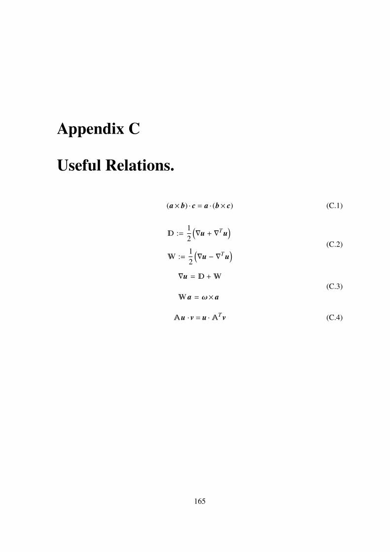
Appendix C
Useful Relations.
(a× b) · c = a · (b× c) (C.1)
:=12
(∇u + ∇T u
) :=
12
(∇u − ∇T u
) (C.2)
∇u = +
a = ω× a(C.3)
u · v = u · T v (C.4)
165

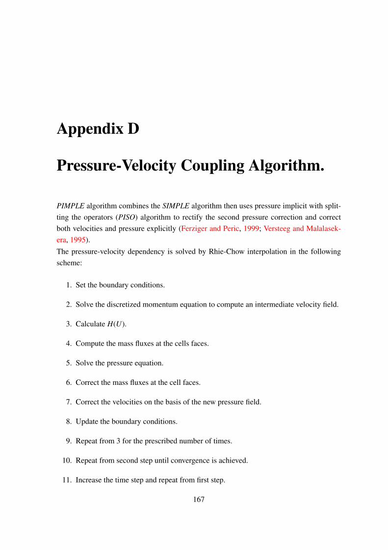
Appendix D
Pressure-Velocity Coupling Algorithm.
PIMPLE algorithm combines the SIMPLE algorithm then uses pressure implicit with split-ting the operators (PISO) algorithm to rectify the second pressure correction and correctboth velocities and pressure explicitly (Ferziger and Peric, 1999; Versteeg and Malalasek-era, 1995).The pressure-velocity dependency is solved by Rhie-Chow interpolation in the followingscheme:
1. Set the boundary conditions.
2. Solve the discretized momentum equation to compute an intermediate velocity field.
3. Calculate H(U).
4. Compute the mass fluxes at the cells faces.
5. Solve the pressure equation.
6. Correct the mass fluxes at the cell faces.
7. Correct the velocities on the basis of the new pressure field.
8. Update the boundary conditions.
9. Repeat from 3 for the prescribed number of times.
10. Repeat from second step until convergence is achieved.
11. Increase the time step and repeat from first step.
167
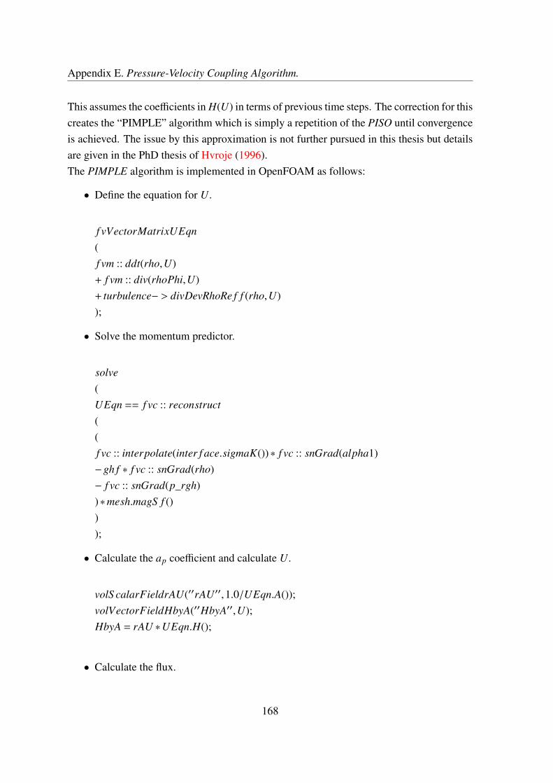
Appendix E. Pressure-Velocity Coupling Algorithm.
This assumes the coefficients in H(U) in terms of previous time steps. The correction for thiscreates the “PIMPLE” algorithm which is simply a repetition of the PISO until convergenceis achieved. The issue by this approximation is not further pursued in this thesis but detailsare given in the PhD thesis of Hvroje (1996).The PIMPLE algorithm is implemented in OpenFOAM as follows:
• Define the equation for U.
f vVectorMatrixUEqn(f vm :: ddt(rho,U)+ f vm :: div(rhoPhi,U)+ turbulence− > divDevRhoRe f f (rho,U));
• Solve the momentum predictor.
solve(UEqn == f vc :: reconstruct((f vc :: interpolate(inter f ace.sigmaK())∗ f vc :: snGrad(alpha1)−gh f ∗ f vc :: snGrad(rho)− f vc :: snGrad(p_rgh))∗mesh.magS f ()));
• Calculate the ap coefficient and calculate U.
volS calarFieldrAU(′′rAU′′,1.0/UEqn.A());volVectorFieldHbyA(′′HbyA′′,U);HbyA = rAU ∗UEqn.H();
• Calculate the flux.
168
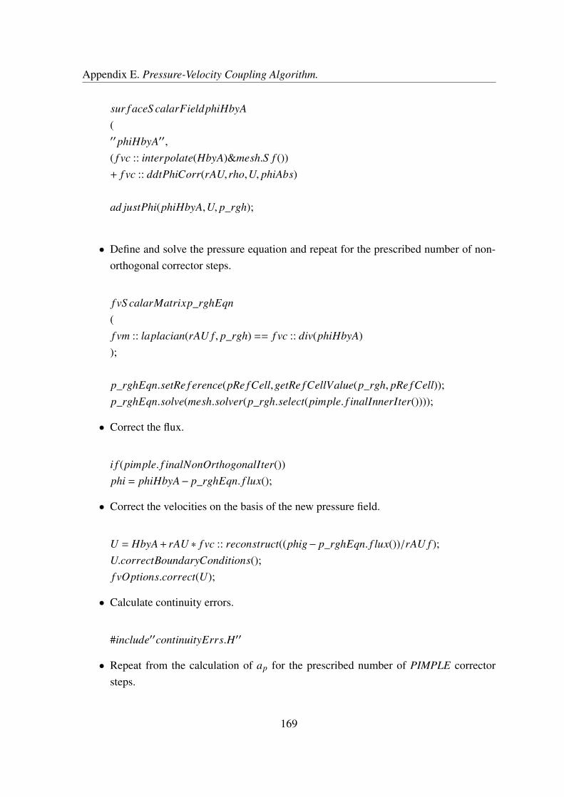
Appendix E. Pressure-Velocity Coupling Algorithm.
sur f aceS calarFieldphiHbyA(′′phiHbyA′′,( f vc :: interpolate(HbyA)&mesh.S f ())+ f vc :: ddtPhiCorr(rAU,rho,U, phiAbs)
ad justPhi(phiHbyA,U, p_rgh);
• Define and solve the pressure equation and repeat for the prescribed number of non-orthogonal corrector steps.
f vS calarMatrixp_rghEqn(f vm :: laplacian(rAU f , p_rgh) == f vc :: div(phiHbyA));
p_rghEqn.setRe f erence(pRe fCell,getRe fCellValue(p_rgh, pRe fCell));p_rghEqn.solve(mesh.solver(p_rgh.select(pimple. f inalInnerIter())));
• Correct the flux.
i f (pimple. f inalNonOrthogonalIter())phi = phiHbyA− p_rghEqn. f lux();
• Correct the velocities on the basis of the new pressure field.
U = HbyA+ rAU ∗ f vc :: reconstruct((phig− p_rghEqn. f lux())/rAU f );U.correctBoundaryConditions();f vOptions.correct(U);
• Calculate continuity errors.
#include′′continuityErrs.H′′
• Repeat from the calculation of ap for the prescribed number of PIMPLE correctorsteps.
169

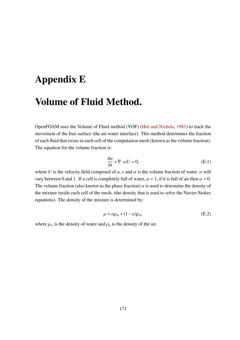
Appendix E
Volume of Fluid Method.
OpenFOAM uses the Volume of Fluid method (VOF) (Hirt and Nichols, 1981) to track themovement of the free surface (the air-water interface). This method determines the fractionof each fluid that exists in each cell of the computation mesh (known as the volume fraction).The equation for the volume fraction is:
∂α
∂t+∇ ·αU = 0, (E.1)
where U is the velocity field composed of u, v and α is the volume fraction of water. α willvary between 0 and 1. If a cell is completely full of water, α = 1, if it is full of air then α = 0.The volume fraction (also known as the phase fraction) α is used to determine the density ofthe mixture inside each cell of the mesh, (the density that is used to solve the Navier-Stokesequations). The density of the mixture is determined by:
ρ = αρw+ (1−α)ρa, (E.2)
where ρw is the density of water and ρa is the density of the air.
171

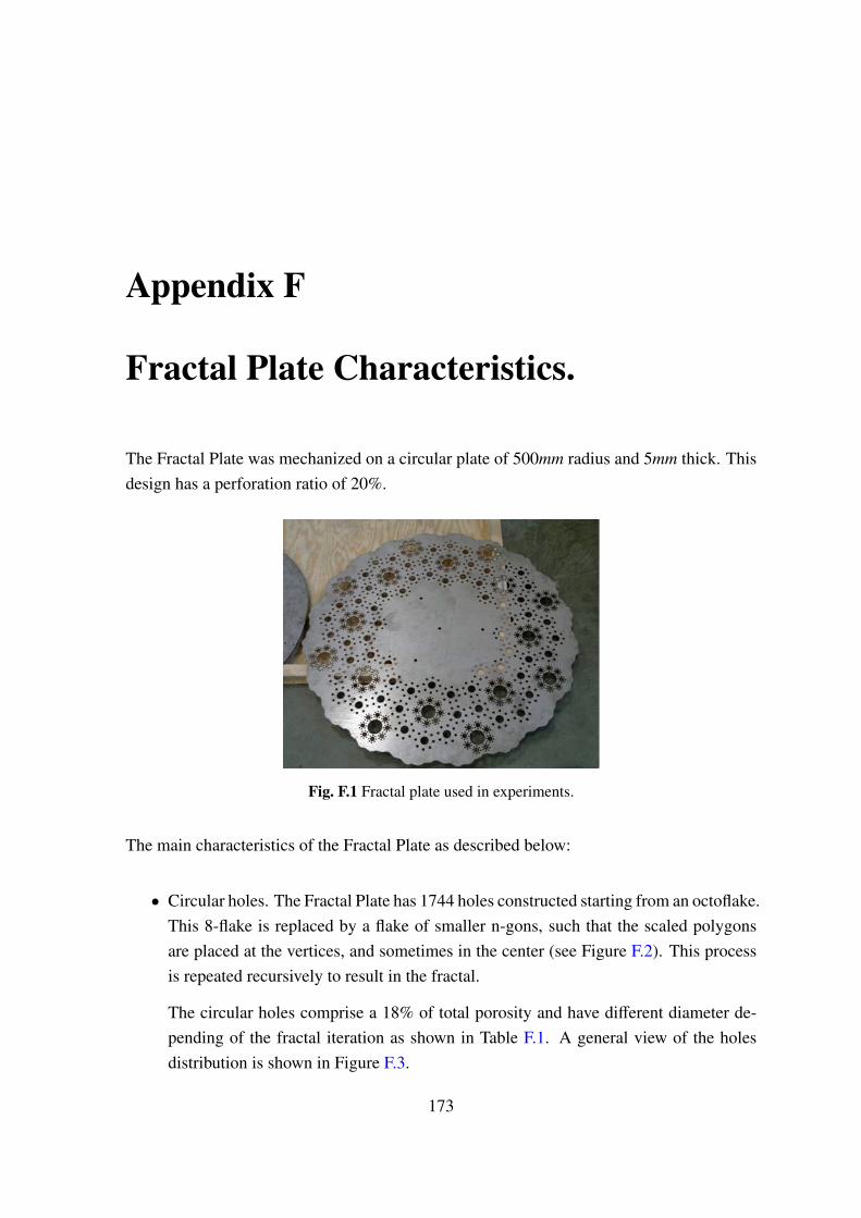
Appendix F
Fractal Plate Characteristics.
The Fractal Plate was mechanized on a circular plate of 500mm radius and 5mm thick. Thisdesign has a perforation ratio of 20%.
Fig. F.1 Fractal plate used in experiments.
The main characteristics of the Fractal Plate as described below:
• Circular holes. The Fractal Plate has 1744 holes constructed starting from an octoflake.This 8-flake is replaced by a flake of smaller n-gons, such that the scaled polygonsare placed at the vertices, and sometimes in the center (see Figure F.2). This processis repeated recursively to result in the fractal.
The circular holes comprise a 18% of total porosity and have different diameter de-pending of the fractal iteration as shown in Table F.1. A general view of the holesdistribution is shown in Figure F.3.
173
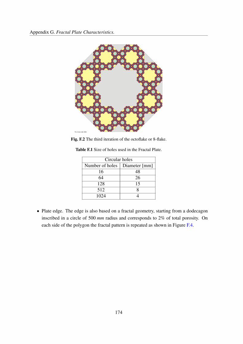
Appendix G. Fractal Plate Characteristics.
Fig. F.2 The third iteration of the octoflake or 8-flake.
Table F.1 Size of holes used in the Fractal Plate.
Circular holesNumber of holes Diameter [mm]
16 4864 26128 15512 8
1024 4
• Plate edge. The edge is also based on a fractal geometry, starting from a dodecagoninscribed in a circle of 500 mm radius and corresponds to 2% of total porosity. Oneach side of the polygon the fractal pattern is repeated as shown in Figure F.4.
174
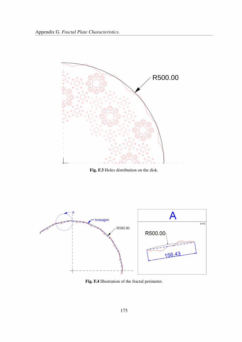
Appendix G. Fractal Plate Characteristics.
R500.00
Fig. F.3 Holes distribution on the disk.
Fig. F.4 Illustration of the fractal perimeter.
175