TECHNICAL REVIEWCharacteristics of the Vold-Kalman Order Tracking Filter

1999

HEADQUARTERS: DK-2850 Nærum · DenmarkTelephone: +45 45 80 05 00 · Fax: +45 45 80 14 05Internet: http://www.bk.dk · e-mail: info@bk.dk

BV

0052

–11

ISSN

000

7–26

21BV0052-11_omslag.qxd 10/02/00 13:50 Page 1

Previously issued numbers ofBrüel & Kjær Technical Review1–1998 Danish Primary Laboratory of Acoustics (DPLA) as Part of the National

Metrology OrganisationPressure Reciprocity Calibration – Instrumentation, Results and UncertaintyMP.EXE, a Calculation Program for Pressure Reciprocity Calibration of Microphones

1–1997 A New Design Principle for Triaxial Piezoelectric AccelerometersA Simple QC Test for Knock SensorsTorsional Operational Deflection Shapes (TODS) Measurements

2–1996 Non-stationary Signal Analysis using Wavelet Transform, Short-time Fourier Transform and Wigner-Ville Distribution

1–1996 Calibration Uncertainties & Distortion of Microphones.Wide Band Intensity Probe. Accelerometer Mounted Resonance Test

2–1995 Order Tracking Analysis1–1995 Use of Spatial Transformation of Sound Fields (STSF) Techniques in the

Automative Industry2–1994 The use of Impulse Response Function for Modal Parameter Estimation

Complex Modulus and Damping Measurements using Resonant and Non-resonant Methods (Damping Part II)

1–1994 Digital Filter Techniques vs. FFT Techniques for Damping Measurements (Damping Part I)

2–1990 Optical Filters and their Use with the Type 1302 & Type 1306 Photoacoustic Gas Monitors

1–1990 The Brüel&Kjær Photoacoustic Transducer System and its Physical Properties

2–1989 STSF — Practical Instrumentation and ApplicationDigital Filter Analysis: Real-time and Non Real-time Performance

1–1989 STSF — A Unique Technique for Scan Based Near-Field Acoustic Holography Without Restrictions on Coherence

2–1988 Quantifying Draught Risk1–1988 Using Experimental Modal Analysis to Simulate Structural Dynamic

ModificationsUse of Operational Deflection Shapes for Noise Control of Discrete Tones

4–1987 Windows to FFT Analysis (Part II)Acoustic Calibrator for Intensity Measurement Systems

3–1987 Windows to FFT Analysis (Part I)2–1987 Recent Developments in Accelerometer Design

Trends in Accelerometer Calibration1–1987 Vibration Monitoring of Machines

(Continued on cover page 3)

TechnicalReviewNo. 1 – 1999

Contents

Characteristics of the Vold-Kalman Order Tracking Filter ....................... 16. Gade, H. Herlufsen, H. Konstantin-Hansen, H. Vold

Copyright © 1999, Brüel & Kjær Sound & Vibration Measurement A/S

All rights reserved. No part of this publication may be reproduced or distributed in any form, or by any means, without prior written permission of the publishers. For details, contact: Brüel & Kjær Sound & Vibration Measurement A/S, DK-2850 Nærum, Denmark.

Editor: Harry K. Zaveri Photographer: Peder Dalmo

Characteristics of the Vold-Kalman OrderTracking Filter

S. Gade, H. Herlufsen, H. Konstantin-Hansen, H. Vold*

AbstractIn this article the filter characteristics of the Vold-Kalman Order Tracking Fil-ter are presented. Both frequency response as well as time response and theirtime-frequency relationship have been investigated. Some guidelines for opti-mum choice of filter parameters are presented.

The Vold-Kalman filter enables high performance simultaneous tracking oforders in systems with multiple independent shafts. With this new filter andusing multiple tacho references, waveforms, as well as amplitude and phasemay be extracted without the beating interactions that are associated withconventional methods. The Vold-Kalman filter provides several filter shapesfor optimum resolution and stop-band suppression. Orders extracted as wave-forms have no phase bias, and may hence be used for playback, synthesis andtailoring.

RésuméCet article présente les caractéristiques du filtrage Vold-Kalman applicablepour les suivis d’ordres. Y sont considérées la réponse en fréquence, la réponsetemporelle et les relations fréquence-temps. Quelques conseils et idées direc-tives sur le paramétrage optimal du filtre y sont également donnés.

Le filtrage Vold-Kalman permet d’effectuer un suivi d’ordres simultané ettrès performant pour l'analyse de systèmes multi-axiaux. Associé à l’utilisa-tion de multi-références tachymétriques, ce nouvel outil permet d’extraire lesdonnées module, phase et formes d’onde sans les perturbations et lesphénomènes de battement observés avec les méthodes conventionnelles.Diverses formes de filtre permettent l'obtention d’une résolution toujours opti-

* Vold Solution Inc., USA

1

male et la suppression de la bande d’arrêt. Extraits comme formes d’onde sanserreur sur la phase, les ordres peuvent être réutilisés pour la relecture, la syn-thèse et l’optimisation des données.

ZusammenfassungDieser Artikel stellt die Filtercharakteristiken des Vold-Kalman-Filters fürOrdnungsanalyse vor. Untersucht wurden Frequenzgang und Zeitcharakter-istik sowie die Zeit-Frequenz-Beziehung. Es werden Hinweise zur optimalenAuswahl von Filterparametern gegeben.

Das Vold-Kalman-Filter erlaubt eine präzise simultane Ordnungsanalyse inSystemen mit mehreren voneinander unabhängig rotierenden Wellen. Mitdem neuen Filter können unter Verwendung mehrerer Referenz-Tachogeberdie Ordnungsverläufe sowie Amplituden und Phasen ohne die mit traditionel-len Methoden verbundenen Schwebungseffekte ermittelt werden. Vold-Kalman liefert verschiedene Filterformen, um optimale Auflösung und Sele-ktivität zu erreichen. Als Wellenformen extrahierte Ordnungen besitzen keinesystematischen Phasenfehler und sind deshalb für Playback, Synthese und“Tailoring” geeignet.

IntroductionVold and Leuridan [1] introduced in 1993 an algorithm for high resolution,slew rate independent order tracking based on the concepts of Kalman filters.Kalman filters have been employed successfully in control and guidance sys-tems since the sixties, with particular applications to avionics and navigation[8,9]. The main feature of the filters is accurately tracking of signals of knownstructure among noise and other signal components with different structure.The new algorithm has been successful as implemented in a commercial soft-ware system in solving data analysis problems previously intractable withother analysis methods. At the same time certain deficiencies have surfaced,prompting the development of an improved formulation, in particular thecapability of being able to control the frequency and the time response of thefilter and to separate close and crossing orders [3].

This article gives an introduction to the new Vold-Kalman algorithm,presents the frequency and time response of the filters and their time-fre-quency relationship and gives some examples of their applications usingPULSE, the Brüel & Kjær, Multi-analyzer System Type 3560 [4].

2

Overview of Methods for Analysis of Non-Stationary SignalsA number of traditional analysis methods can be used for the analysis of non-stationary signals and they can roughly be categorized as follows:

1) Divide into Quasi-stationary segments by proper selection of analysiswindowa) Record the signal in a time buffer (or on disk) and analyze after-

wards: Scan Analysisb) Analyze on-line and store the spectra for later presentation and

post-processing: Multifunction/multibuffer measurements 2) Analyze individual events in a cycle of a signal and average over several

cycles: Gated measurements and analysis3) Sample the signal according to its frequency/RPM variations (adaptive

data resampling): Order tracking measurements4) Analysis using Autoregressive Signal Modelling: Maximum Entropy

Spectral Analysis [11].The procedure used for Vold-Kalman order tracking analysis (adaptive fil-

tering, where the presumed model of the signal is not fixed in time or fre-quency content, but automatically adapts itself as the speed of the deviceunder test changes) is as described in 1a) above, i.e. a post-processing proce-dure based on time data.

Order Tracking AnalysisOrder tracking is the art and science of extracting the sinusoidal content ofmeasurements from acousto-mechanical systems under periodic loading/exci-tation. Order tracking is used for troubleshooting, design and synthesis [5, 18].

Each periodic loading produces sinusoidal overtones, or orders/harmonics, atfrequencies that are multiples of that of the fundamental tone (RPM). Theorders may be regarded as amplitude and phase modulated carrier waves thatvary in frequency. Many practical systems have multiple shafts that may runcoherently through fixed transmissions, or partially related through belt slip-page and control loops, or independently, such as when a cooling fan operatesin an engine compartment.

In order analysis we focus on machine revolutions rather than on time as thebase for the signal analysis. Thus in the spectrum domain the focus is onorders rather than frequency components.

3

Traditional Analysis Techniques for Run-up/Run-down TestsOne of the main applications of order tracking is analysis of run-ups and run-downs. Investigation of the system responses and dynamic behaviour at thevarious rotational speeds is a key element in design, troubleshooting, producttesting and quality control. Depending on the information required from thetest, different analysis techniques can be applied.

The most simple is determination of the acoustic response in terms of theoverall Linear, A, B or C weighted level as a function of RPM. This is often usedin product testing for comparison with reference (tolerance) curves. No diagnos-tic information is obtained.

“Next level” of analysis is the inclusion of spectral information. In acoustictesting 1/1-octave or 1/3-octave spectra are often used in order to get the spectralcontent in constant percentage filter bands as a function of rotational speed (con-stant percentage bandwidth means that the bandwidth is proportional with thefrequency). These can reveal frequency regions with annoying resonances andthey relate to the human perception of the radiated noise. Information about theindividual orders cannot be extracted except for the lowest harmonics with 1/3-octave filters. Fig.1 shows the contour plot of the acoustic response during a run-up of a motor analyzed in 1/3-octaves. The 1st (and to some degree the 2nd) orderis identified together with regions of high response levels. Fig.2 shows the over-all level as well as some individual 1/3-octave bands as a function of RPM. Moreinformation about the lower harmonic order components could be obtained bygoing to for example 1/12-octave filter bandwidth. Real-time 1/12-octave filters,however, require more DSP (Digital Signal Processing) power in the system.

More advanced acoustic processing is to use a Loudness Analyzer and storenon-stationary Specific Loudness as a function of RPM, [14]. Non-stationaryLoudness gives a much better model of the human hearing system and takesinto account that the sensitivity of the human ear is not the same for all frequen-cies and levels as well as the effect of temporal and frequency masking.

In order to resolve the various orders in the frequency domain, narrowbandfrequency spectra (FFT without tracking) could be applied. FFT gives the spec-tral information in constant bandwidth (same bandwidth at all frequencies andRPMs) and facilitates identification of harmonic families when presented on alinear frequency axis. This enables diagnosis and source identification.Theadvantage of using FFT without tracking is that it does not cost very much interms of DSP power. Another advantage is that one FFT analyzer can relate theanalysis to more tacho signals: multi-shaft analysis. A disadvantage is that

4

Fig. 1. 1/3-octave colour contour plot (maximum interpolation used) of the acousticresponse during run-up

Fig. 2. Selected 1/3-octave bands and overall linear level of acoustic response as functionsof RPM

the smearing of the individual (and especially the higher) order components inthe frequency spectra will appear if the run-up/run-down is fast. This is dueto the fact that each FFT spectrum represents a certain time window andtherefore a certain change of the rotational speed. Another aspect is thatrather large Fourier transforms (many lines in the FFT) are required in caseswhere the test is running over a wide speed (RPM) range and higher harmon-ics have to be included in the analysis. Example: RPM range from 600RPM(10Hz) to 6000RPM (100Hz), 16 orders included in the spectra (i.e. min. 16 x100Hz = 1.6kHz frequency span) and a resolution of 2Hz (5 FFT lines per

5

order at 600RPM) will require 800FFT lines in the analysis (2Hz resolutionwith a frequency span of 1.6kHz).

Fig.3 shows the contour plot of an FFT analysis of the same acousticresponse as in Fig.1. The harmonic family of the fundamental periodic loadingis easily identified. Resonance frequencies excited by the various harmonicorders appear on vertical lines parallel to the RPM axis. Fig.4 shows the first 4harmonics and the total level in the selected frequency span, as a function ofRPM. This information is obtained by slicing in the contour plot (post-proc-essed in “real-time” during the test) or by pre-processing, i.e. directly measuredby the FFT analyzer during the run-up/run-down. Both order – as well as fre-quency-slices can be measured/extracted using these methods.

Fig. 3. Contour plot of the FFT spectra of the acoustic response as function of RPM

Fig. 4. Selected orders and total level (in the frequency span) as functions of RPM

6

The above mentioned disadvantages can be overcome by use of tracking.The tracking technique uses the instantaneous RPM values for calculation ofthe samples referenced to the revolution of the rotating shafts instead of thetime clock, see e.g. [5]. Fourier transform of the revolution based samplesresults in order spectra instead of frequency spectra and harmonic ordersrelated to the measured RPM remains in fixed lines in the order spectrum.This means that smearing of the order related components is avoided andorder components, which might have been smeared out in a frequency spec-trum, can be identified. The number of lines required in the order spectra for acertain test is less than the number of lines needed if frequency spectra wereused. Example: 20 orders is analyzed with a resolution of 0.2 order (5 lines perorder, giving possibility to identify inter-harmonic components) by use of 100line order spectra independent of the speed range. The price to pay is that thereal-time tracking algorithms require more DSP power than the “normal”FFT analysis.

Fig.5 shows the contour plot of order spectra of the same acoustic responseas in Fig.1 and Fig.3. The orders appear on vertical lines parallel to the RPMaxis whereas resonances appear on hyperbolic curves (fixed frequency curvesindicated by the cursor). Slices of the first 10 harmonics and the total level asa function of RPM is shown (as a waterfall plot) in Fig.6. The order sliceresults obtained by the frequency analysis and the order analysis are thesame.

In product testing there is often a requirement of having the results in real-time (on-line) containing information of both individual orders, overall levels(Linear, A, B or C weighted) and in some cases 1/1- or 1/3-octave bands as well.This can only be obtained using a combination of the mentioned techniques.The key issue, in order to reduce the test time and have consistency of data inthe various analyses is to perform the analyses simultaneously. This is thecase in the results illustrated in Fig.1 through Fig.6 where the Brüel&KjærPULSE, Multi-analyzer System Type 3560 is used. Four analyzers are used inparallel: A tachometer (for RPM calculations), a 1/3-octave analyzer (1/3-octaves and overall levels), an FFT analyzer (frequency spectra) and an orderanalyzer (order spectra) giving all the results simultaneously. A loudness ana-lyzer can be included as well. In this example only one tachometer signal isused. In multiaxle applications the different tachometer signals should beapplied to the tachometer. The scaling of the RPM axis and the calculation ofthe order slices can then be referenced to the different rotation speeds (RPMs).If tracking is used (as in Fig. 5 and Fig. 6) an order analyzer would have to bedefined for each reference tachometer signal.

7

Fig. 5. Contour plot of real-time order tracking spectra (resampling technique) of theacoustic response

Fig. 6. First 10 harmonics and the total level (in the span of 20 orders), from real-timeorder tracking spectra, as functions of RPM (shown as a waterfall plot)

These analysis techniques can be applied in real-time (on-line) whichmeans that the results are obtained during the test. They are based upon con-ventional frequency (Fourier) analysis that means that the resolution in thetime domain is linked to the resolution in the frequency domain and viceversa. This gives a limitation of how accurate phenomena can be identified inboth domains in the same analysis. This is also referred to as the uncertaintyprinciple. For FFT analysis the relation is written as ∆f × T =1, where T is therecord length (“resolution” in time domain) and ∆f is the line spacing in thespectrum (“resolution” in frequency domain). If the changes in the signals are

8

too rapid we will not be able to follow (analyze) these changes using thesetechniques. The real-time order tracking technique, mentioned above, is basedon resampling and there is a limitation of how fast the speed (RPM) is allowedto change (also called slew rate limitation).

These limitations are examples of where the Vold-Kalman tracking filtercan be used, rendering a comprehensive set of analysis tools. It minimizes theresolution problems and has no slew rate limitations.

Applications of Vold-Kalman Order Tracking FilteringThe Vold-Kalman algorithm enables simultaneous estimation of multipleorders, effectively decoupling close and crossing orders, e.g., separating driveshaft orders from wheel orders in suspension tuning. Decoupling is especiallyimportant for acoustics applications, where order crossings cause transientbeating events. The new algorithm allows for a much wider range of filtershapes, such that signals with sideband modulations are processed with highfidelity. Finally, systems subject to radical RPM changes, such as transmis-sions, are tracked also through the transient events (e.g. gear shifts) associ-ated with abrupt changes in inertia and boundary conditions. The goal oforder tracking is to extract selected orders in terms of amplitude and phase,called Complex Orders or Phase Assigned Orders, or as waveforms. The orderfunctions are extracted without time delay (no phase shift), and may hence beused in synthesis applications for sound quality, e.g. removal of nuisanceorders and laboratory simulations. Other applications include multiplane bal-ancing, and measurements of Operational Deflection Shapes, ODS.

Fundamental Notions and EquationsMechanical systems under periodic loading, such as those with one or morerotating shafts will respond in measurements with a superposition of sinewaves whose frequencies are integer multiples of the fundamental excitationfrequencies. Notice that this also applies to the limit cycle response of non-lin-ear systems. As the periodic loadings change their speed, the responses willalso change their frequencies accordingly. Since mechanical systems normallyhave transfer characteristics dependent upon frequency, the amplitude andphase of these sine waves will typically also change as the periodic loadingschange their speed. The sine waves whose frequencies are constant multiples

9

of an underlying periodic loading are said to be harmonics or orders of thatloading, also when the multiple is fractional due to gears or belt drives.

It is often helpful to visualize an order as an amplitude/phase modulatedradio signal. The underlying sine wave whose frequency is a multiple of thefundamental periodic phenomenon would be the carrier wave, while theslowly varying amplitude and phase function that modulates the carrier waveis the radio program. A radio receiver demodulates the signal by removing thecarrier wave and playing the modulation function, also known as the (com-plex) envelope. Now, in mechanical systems, the carrier wave may continuallychange its frequency, making the orders similar to amplitude modulatedspread spectrum radio signals.

The goal of order tracking is to extract selected orders in terms of amplitudeand phase or as real time series. These entities will in general be estimated asfunctions of time to allow for any pattern of speed or axle RPM variations.

Phasors and Complex EnvelopesThe carrier wave of an order can be visualised as a phasor, which is a complexoscillator with an instantaneous frequency proportional to a constant multipleof the underlying axle speed as in the equation

(1)

where the integral of frequency gives the angle travelled by the axle up to thecurrent time, k is the order number and . Note that the phasor isalways on the complex unit circle.

The amplitude modulated complex order is now given as the productAk(t) Θk(t) where Ak(t) is the complex envelope. These complex orders mustoccur in complex conjugate pairs to sum to a real signal, such that the totalsuperposition X(t) of orders relative to an axle can be written as

(2)

where k runs over all positive and negative multiples of the underlying axlespeed.

Θk t( ) exp 2πki f u( ) ud0

t

∫

=

i 1–=

X t( ) Ak t( )Θk t( )

k∑=

10

Time Variant ZoomThe expression for the phasor (1) implies the functional relationship

(3)

In particular, inspection of equation (1) shows that Θ0(t) ≡ 1. When the axlespeed has been estimated as a function of time, equations (2) and (3) thenshow that we can centre a designated order at DC (zero frequency) by the timevariant zoom transform

(4)

The low frequency complex envelope Aj(t) has now been straightened, andmay, for example, be extracted in the time domain by any suitable lowpass fil-ter. This super-heterodyning process is similar to the tracking of an amplitudemodulated spread spectrum radio source.

Using traditional tracking algorithms the centre frequency of a bandpasstracking filter is controlled by the instantaneous RPM. The filter AC output isthen detected (squared and averaged) into a “slowly” varying DC using, forexample, a traditional RMS detector, with all its well known limitations,among those – averaging time dependent ripple in the output as well as loss ofphase information. For the Vold-Kalman processing, the order of interest isfrequency shifted (or zoomed) to DC, a shift which is controlled by the instan-taneous RPM and then followed by a lowpass filtration which replaces thebandpass filtering process. Thus there is no need for any further detection; i.e.the Vold-Kalman filtration includes a simultaneous envelope detection of bothmagnitude and phase. Order Waveforms are then obtained by remodulatingthe complex orders by the order frequency carrier wave (given by the RPMprofile), i.e. the complex orders are heterodyned from DC to its original fre-quency location.

Vold-Kalman FilterThe basic idea behind the Vold-Kalman filter is to define local constraints thatstate that the unknown complex envelopes are smooth and that the sum ofthe orders should approximate the total measured signal. The smoothness

Θk t( )Θj t( ) Θk j+ t( )=

Θ j– t( )X t( ) Aj t( ) Ak t( )Θk j– t( )

k j≠∑+=

11

condition is called the structural equation, and the relationship with themeasured data is called the data equation. The somewhat ambiguous notationX(n∆t) = X(n), where ∆t is the sampling time increment, is used in this articleto simplify the mathematical exposition.

Structural EquationsThe complex envelope Aj(t) is the low frequency modulation of the carrierwave Θj(t). Low frequency entails smoothness, and one sufficient condition forsmoothness is that the function locally can be represented by a low order poly-nomial. This condition can be expressed in continuous time using multiple dif-ferentiation as

(5)

where ε(t) represents higher order terms. The same constraint can be appliedto sampled data by using the difference operator such that

(6)

Note that the difference operator of a given order annihilates all polynomi-als of one order less. Equation (6) is called the structural equation when theright hand side ~ε(n) is regarded as noise or error. This complex equation willbe satisfied in an approximate sense for all discrete time points in the dataset.

The structural difference equation in the first generation of the Vold-Kalman algorithm is a real second order equation for the real modulatedwaveform

(7)

that requires a demodulation through the Vandermonde equations to find theamplitude and phase, see [1]. This operator also only annihilates the constantpolynomial.

dsAj t( )

dts------------------- ε t( )=

∇sAj n( ) ε̃ n( )=

Xj n( ) 2Re Aj n( )Θj n( )( )=

12

Data EquationThe structural equation only enforces the smoothness conditions on the esti-mates of the complex envelopes, such that we need an equation that relatesthe estimates to the measured data. The simplest such condition is to statethat the sum of the orders differs only by an error term from the measureddata as expressed in the equation

(8)

where the summation is for a desired subset of orders.The above equation (8) is called the data equation when the right-hand side

is regarded as noise or error. This equation will also be enforced in anapproximate sense for all sampled data points.

DecouplingWhen several orders are estimated simultaneously, equation (8) ensures thatthe total signal energy will be distributed between these orders, and togetherwith the smoothness conditions of the structural equation (6) this enforces adecoupling of close and crossing orders as is demonstrated in the examples.The mathematics of this procedure is quite analogous to the repeated rootproblem in modal analysis, see, [7]. When orders coincide in frequency over anextended time segment, the allocation of energy to such orders is poorlydefined, and numerical ill conditioning may ensue. Widening the filter band-width is one possible remedy in this case.

Example of Tacho ProcessingAny method with high resolution needs proper controls, and for the Vold-Kalman filter this means a very accurate estimation of the instantaneousRPM such that the tracking filter will follow the peak of the order functionsinstead of extracting data from the foothills. The methodology that has beenchosen for the Vold-Kalman filter is that of fitting cubic splines in a leastsquares sense to the table of level crossings from a tacho waveform. Choice ofother possible methods is discussed in [1]. Tacho processing is explained inmore details later.

X n( ) Aj n( )Θj n( )

j J∈∑– δ̃ n( )=

δ̃ n( )

13

Fig. 7. Corrupted tacho waveform, Run-down from 5200 RPM to 400 RPM

Fig. 8. Raw data and spline fit

14

The spline fit enables automatic rejection of outlying data points with a sub-sequent refit on a censored table of level crossings. The spline fit and censoringprocess capability is illustrated by the corrupted tachometer signal from a5200RPM to 400RPM run-down lasting for about 15s. There are three drop-outs with a total duration of 15% of the total measurement time as shown inFig.7. The raw level crossing table and spline fit without rejection is shown inFig.8. The fitted data is then compared with the raw table, the largest deviants(in this case 1% of the raw RPM table has been specified for rejection) are cen-sored and a refit is performed, with the clean results depicted in Fig. 9. As aresult the three “wild” RPM points have been removed and the spline fit is suf-ficiently stiff to straddle the empty sections. This is a fully automatic process,often obviating the need for manual tacho signal repair. Notice that the rawRPM profiles have been drawn as curves, i.e. with straight-line connectionsbetween the table values, both without and with rejections shown in Figs.8 & 9.

Fig. 9. Censored Data with Corrected Spline Fit (curves offset for ease of comparison)

15

Vold-Kalman Filter Process, Step by Step – an ExampleTo illustrate the ease of use of the Vold-Kalman filter process as implementedin the Brüel&Kjær PULSE, Multi-analysis System Type 3560, a run-upmeasurement on a small single shaft electrical motor has been performed.Fig. 10 shows the vibration response signal, which was recorded together witha tacho signal. A 1.6kHz frequency range and a total recording of 20s havebeen selected using a PULSE Time Capture Analyzer [17]. The number ofsamples recorded is 81 920 in each channel. 18s of the recorded signal wasextracted for Vold-Kalman tracking using a delta cursor.

Fig. 10. Vibration time signal of the run-up

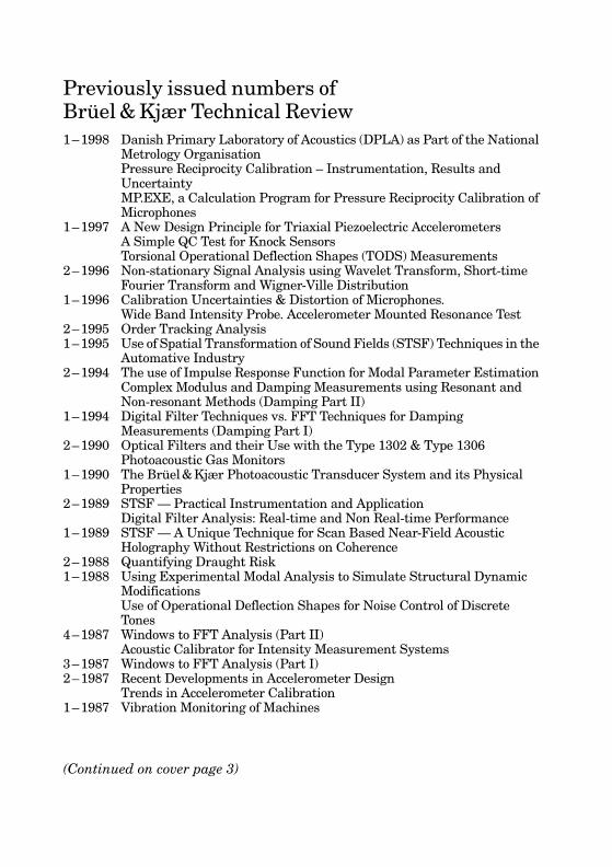
a) Overview of the Event using Fourier AnalysisThe first step is to use conventional techniques in order to gain some insightin the harmonic orders of interest, gearshifts etc. Fig. 11 shows a contour plotof an STFT (Short Time Fourier Transform) of the vibration signal. The recordlength of each transform is set to 125ms (512 samples) resulting in 200 linesin the frequency domain (line spacing ∆f of 8 Hz). An overlap of 66% is usedresulting in a multi-buffer of 500 spectra covering the selected 18s. From thecontour plot it is revealed that the dominating orders are nos. 1, 3, 9 and 10and as expected, no gearshift is present.

16

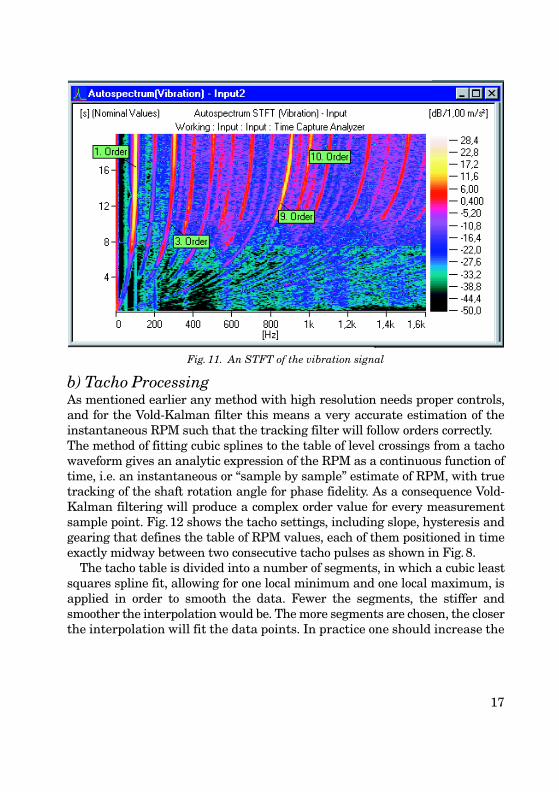
Fig. 11. An STFT of the vibration signal

b) Tacho ProcessingAs mentioned earlier any method with high resolution needs proper controls,and for the Vold-Kalman filter this means a very accurate estimation of theinstantaneous RPM such that the tracking filter will follow orders correctly. The method of fitting cubic splines to the table of level crossings from a tachowaveform gives an analytic expression of the RPM as a continuous function oftime, i.e. an instantaneous or “sample by sample” estimate of RPM, with truetracking of the shaft rotation angle for phase fidelity. As a consequence Vold-Kalman filtering will produce a complex order value for every measurementsample point. Fig.12 shows the tacho settings, including slope, hysteresis andgearing that defines the table of RPM values, each of them positioned in timeexactly midway between two consecutive tacho pulses as shown in Fig.8.

The tacho table is divided into a number of segments, in which a cubic leastsquares spline fit, allowing for one local minimum and one local maximum, isapplied in order to smooth the data. Fewer the segments, the stiffer andsmoother the interpolation would be. The more segments are chosen, the closerthe interpolation will fit the data points. In practice one should increase the

17

Fig. 12. Tacho setting property page

number of segments until a reasonable match to the raw RPM is obtained. Toomany segments might fit non-physical variations (noise) in the raw RPM.Continuity and first derivative continuity constraint requirement is appliedbetween segments. There is also the option of specifying hinge points (singu-lar events) in the spline fit, such that sudden changes in inertial propertiescan be tracked, as in the case of clutching and gearshifts by relaxing the firstderivative continuity at shift points. The operator identifies the exact loca-tions of hinge points by expanding the RPM profiles for detailed visual inspec-tion.

The spline fit also permits automatic rejection of outlying data points(such as tacho dropouts) with a subsequent refit on a censored table of levelcrossings as mentioned earlier. The Curve Fit property page is shown inFig. 13.

18

Fig. 13. Tacho table Curve Fit property page

Fig. 14. Comparison of the measured (raw, tabular) and curve fitted RPM profiles

Fig.14 shows a superimposed graph of the measured and the curve fittedRPM profiles. The maximum slew rate in this case is seen to be approximately800RPM/s and the range is between 1000RPM and 6000RPM.

19

c) Vold-Kalman Filtering

Fig. 15. Vold-Kalman filter property page

Orders can now be extracted from the signal in terms of waveforms or as PhaseAssigned Orders (Complex Orders).

The Vold-Kalman filter property page is shown in Fig.15. The computationalcomplexity of the Vold-Kalman filter is proportional to the number of time sam-ples and to the number of orders to be extracted, but also to some degreedepends on filter type, output, bandwidth and decimation. For example, thecomputation time for a three-pole filter is 10% longer than for a two-pole filter.

When decoupling is used, however, the computational cost can be high, sinceconstraint conditions are being enforced between the order function estimates.

Fig.16 shows the waveform of the 1st, 3rd, 9th and 10th order extractedusing a two-pole Vold-Kalman filter with a bandwidth of 10% (i.e. 10% of thefundamental frequency). Extracted waveforms can be played via a sound cardand they can be exported as wave files. Sound Quality application is an exam-ple were this is very useful.

20

Fig. 16. Waveforms of the 1st, 3rd, 9th and 10th Order, extracted using a two-pole Vold-Kalman filter with 10% bandwidth

Fig. 17. Magnitude of the 4 most dominating orders as a function of time, extracted usinga two-pole Vold-Kalman filter with 10% bandwidth

21

Extracted as Phase Assigned Orders means that the orders are determinedin terms of magnitude and phase. Fig.17 shows the magnitude of the PhaseAssigned Orders of the 1st, 3rd, 9th and 10th order, which were the 4 mostdominating orders. A two-pole Vold-Kalman filter with a bandwidth of 10% isused. It should be noted that the phase of the orders is highly sensitive tochoice of filter bandwidth for time sections with poor signal to noise ratio. Thisis most evident when displaying unwrapped phase.

The Vold-Kalman analysis is a time-based analysis yielding results, PhaseAssigned Orders and Waveforms as a function of time. Often it is desirable toplot the Phase Assigned Orders as a function of RPM, which can be easilydone by exporting the order of interest and the RPM-profile to a spreadsheet.The magnitude of the first order is shown in Fig.18 using MS Excel. The deci-mation features shown in Figs.12 and 15 are used in this case in order toreduce the amount of data to a size, which can be handled by a spreadsheet.

Fig. 18. Magnitude of the first order as a function of RPM, extracted using a two-poleVold-Kalman filter with 10% bandwidth and plotted via MS Excel spreadsheet

Filter Characteristics in Frequency DomainBandwidth selection is done in terms of constant frequency bandwidth or pro-portional to RPM bandwidth (i.e. constant percentage bandwidth). The band-width specification in the Brüel&Kjær Vold-Kalman implementation [16] isin terms of the half – power points, i.e. 3dB bandwidth. Bandwidth propor-tional to RPM is recommended for the analysis of higher harmonic orders oranalysis of wide RPM ranges.

22

The filter shape is measured by sweeping a sine wave through a Vold-Kalman filter with a fixed centre frequency and fixed bandwidth. A sweep rateof 1Hz/s is used for measuring the filter shapes, shown in Fig.19, of a Vold-Kalman filter with a centre frequency of 100Hz and a bandwidth of 8Hz. The x-axis, which is a time axis scaled in seconds, can directly be interpreted as a fre-quency axis scaled in Hz (with a fixed offset). It is seen that a one-pole filter hasvery poor selectivity, a two-pole filter has a much better selectivity, whereas athree-pole filter provides the best selectivity. The 60dB shape factor, i.e. theratio between the 60dB bandwidth and the 3dB bandwidth is often used fordescribing the selectivity of a filter. The 60dB shape factor has been measuredfor the one-, two- and three-pole filters for bandwidths in the range from0.125Hz to 16Hz. These tests showed that the 60dB shape factor for a givenpole specification increases slightly as a function of bandwidth. The one-pole fil-ter has a 60dB shape factor of approximately 50 (variation from 48.8 to 50.8).The two-pole filter has a 60dB shape factor of approximately 7.0 (variation from6.80 to 7.07) and the three-pole filter has a 60dB shape factor of approximately3.6 (variation from 3.58 to 3.68). Thus the selectivity of the three-pole filter istwice as good as the two-pole filter and 14 times better than the one-pole filter.Good selectivity is important to avoid interference (or leakage) between orders.

Fig. 19. Comparison of filter shapes for one-, two- and three-pole Vold-Kalman filters witha bandwidth of 8 Hz

23

Fig. 20. Comparison of the frequency response in the passband for one-, two- and three-pole Vold-Kalman filters with the same bandwidth of 8 Hz

Another characteristic of the filter is the frequency response within thepassband. As seen in Fig.20 the two- and three-pole filters have a much flatterfrequency response in the passband compared to the one-pole filter, with thethree-pole filter having the flattest frequency response. The flatness of the fre-quency response in the passband is important when analyzing the amplitudeand phase modulation of the harmonic carrier frequency. Amplitude andphase modulation corresponds in the frequency domain to sidebands centeredaround the harmonic carrier frequency component, which means that themore flat the frequency response is the more correct the modulation will showup the filter analysis.

The phase of the Frequency Responses for the different filter types is zero inthe full frequency range within the measurable dynamic range. Thus there isno phase distortion or time delay for tracked orders including modulationsidentified as lower and upper sidebands.

24

Filter Characteristics in Time DomainThe time response of Vold-Kalman filters is important to understand whenanalyzing transient phenomena and responses to lightly damped resonancesbeing excited during a run-up or a run-down. The time response has beeninvestigated by applying a tone burst with a certain duration to a Vold-Kalman filter with a fixed centre frequency corresponding to the frequency ofthe toneburst. In Fig.21 the magnitude (envelope) of the response of a filtercentered at 100Hz with a bandwidth of 8Hz is shown using a logarithmic y-axis. A 100Hz tone burst with a duration of 1s is applied to the filter. Onevery important feature is that the time response is symmetrical in time, i.e. itappears to behave like a non-causal filter. This is because Vold-Kalman filter-ing is implemented as post processing allowing for non-causal filter imple-mentation and extraction of order waveforms with no phase bias or distortion,i.e. without a time delay. Fig.21 shows the time response for one-, two- andthree-pole filters with a bandwidth of 8Hz.

The one-pole filter has, as expected, the shortest decay time and an expo-nential decay which appears as a straight line when displayed with a logarith-mic y-axis, while the two-pole and three-pole filters in addition to the longer

Fig. 21. Comparison of the magnitude of the time responses for one-, two- and three-poleVold-Kalman filters with a bandwidth of 8 Hz. The applied signal, a tone burst of 1 s dura-tion, is shown as well

25

Fig. 22. Comparison of Time Responses for one-pole 2 Hz, 4 Hz and 8 Hz bandwidth Vold-Kalman filters. The applied signal is a tone burst of 1 s duration

decay times also show some lobes. The main lobes of all three filter types showon the other hand nearly the same progress in the upper 25dB, i.e. the same“early decay”, which means their behaviour in terms of how fast they can fol-low amplitude changes of orders are nearly identical.

Fig. 22 shows the time response of a one-pole filter for 3 different choices offilter bandwidths. As expected the decay time is inversely proportional to thebandwidth. Since the slope for a one-pole filter is very similar to the slope ofthe early decay for two- and three-pole filters with the same bandwidth wecan extract the following important time-frequency relationship for all threetypes of Vold-Kalman filters,

B3dB × τ = 0.2 (9)

where B3dB is the 3dB bandwidth of the Vold-Kalman filter and τ is the timeit takes for the time response to decay 8.69dB ( = 10 × log e2). One pole filter isbased on a second order structural equation, i.e. a one degree of freedom reso-nator (an SDOF system) which has the time-frequency relationship, σ × τ = 1(see Ref. [19]) corresponding to B3dB × τ = 1/π. Thus we have an optimum time-

26

frequency relationship close to the Heisenberg’s uncertainty limit using Vold-Kalman filtering. Due to its symmetry the efficient duration of the timeresponse has to be considered 2τ rather than τ. If reverberation time T60instead of time constant τ is preferred, the relation (9) becomes,

B3dB × T60 = 1.4 (10)

When zooming in around the beginning or the end of the tone burst a differ-ence between the three filter types is revealed as seen in Fig. 23. The one-polefilter has a smooth decay before the stop of the tone burst, whereas the two-pole and the three-pole filters show a ripple with a maximum deviation (over-shoot) from the steady state response of 0.28dB and 0.46dB respectively. Thisovershoot phenomenon is only seen in analysis results when analyzing signalswith abrupt amplitude changes (such as in the case of a tone burst) or when atoo narrow filter bandwidth is selected for the analysis (i.e., the time constant,τ of the filter is too long for the signal to be analyzed).

As an additional observation, all time responses have decayed to –6dB, irre-spective of the chosen filter parameters, at the location where the tone burst stops,

Fig. 23. Detailed picture of the time response of the one-, two- and three-pole filters at theend of the tone burst

27

see Figs. 21 and 22. (i.e. where the energy of the order signal inside the ana-lyzed time window is reduced by 3dB). Due to the sudden change in thenature of the signal, from a sine wave to nothing, a further leakage of theorder, into neighbouring frequencies by 3dB is seen. A similar effect isobserved using FFT analysis. See Appendix A fore more details.

The phase curve is zero degrees in the full time range where the time burstexists as expected, except for some small edge effects (less than 1 degree forthe 8Hz fillter) at the two discontinuities, i.e., the Vold-Kalman filter has notime delay for a tracked signal.

Phase of Orders and WaveformsThe major question is: What is the reference for the detected phase? For thePhase Assigned Autospectrum in PULSE, the phase spectrum assigned to theautospectrum is the phase of the cross-spectrum between the selected signaland the reference signal selected by the user, e.g. a tacho signal or any othersuitable signal. This is a typical dual channel measurement.

For the Vold-Kalman filtering the situation is slightly different, the phaseis extracted from the vibration/acoustic signal itself, i.e. from one signal only:

In a time domain model the Vold-Kalman filter fits sine waves at theselected order/carrier frequency to the vibration/acoustic signal. For a one-pole filter three data samples are fitted at a time in a recursive manner [2,20]. For two and three pole filters more samples are used in the curve fit/filtering process.

The phase of a particular Phase Assigned Order component at time zero(beginning of time record) will be the phase at time zero for the curve fitted sinewave result, similar to the phase of a sine wave component in a Fourier Spec-trum which is the phase of this component at the beginning of the time record.The standard convention is as follows: if a sine wave has its maximum ampli-tude at time zero, then the phase of its Fourier component is per definition 0degrees. If a sine wave has its minimum amplitude at time zero, then the phaseis 180 degrees. For zero crossings with positive and negative slopes the phase isminus 90 and plus 90 degrees respectively. Thus the starting phase for a PhaseAssigned Order is the phase of the order signal itself irrespective of the actualstarting phase of the tacho reference / carrier / RPM signal. This is also a conse-quence of the fact that only the RPM profile (i.e., frequency) and not phase isderived from the tacho signal. The phase of the tacho reference/carrier/RPMsignal can then be regarded to have zero phase at time zero for any order ofinterest, and the phase for any order is thus assigned to the phase of the rotat-

28

ing shaft, i.e. the tacho signal with an arbitrary offset. The phase at any latertime for the Phase Assigned Orders depends on the transfer propertiesbetween the forcing functions from the rotating shaft to the measurement/observation position.

When calculating the order waveform from the Phase Assigned Orders andthe RPM, the order waveform will have a phase at time zero which is the com-bination of the phase of the carrier wave (per definition 0 degrees) and thephase of the phase assigned order at time zero, which is the measured phase ofthe order waveform at time zero. Thus the output order waveform will have nophase shift, i.e. no time delay, with respect to the measured signal and thus canbe used in synthesis studies as shown later.

Selection of Bandwidth and Filter TypeSelection of the filter bandwidth is basically a compromise between having abandwidth which is sufficiently narrow to separate the various order compo-nents in the signal and a bandwidth which is sufficiently wide, i.e. giving asufficiently short filter response time, in order to follow the changes in the sig-nal amplitude. The contour plot of the STFT analysis can be used for evaluat-ing the separation of the various components. Using the radio signal analogythis means that not only the carrier frequency located at the centre frequencyof the filter, but also the AM/FM modulation components should be inside thefilter passband, since it is these components that contain the information ofinterest. An extremely narrow filter that suppresses all the sidebands wouldproduce an order with constant magnitude as a function of time and constantslope of the phase.

Various research tests have shown that when orders pass through a reso-nance the time constant of the filter, τ, should be shorter than 1/10 of the time,T3dB , it takes for the particular order to sweep through the 3dB bandwidth ofthe resonance, ∆ f3dB. This ensures an error of less than 0.5dB of the peakamplitude at the resonance using a one-pole filter. For two- and three-pole fil-ters the error of the measured peak will be less. If no resonance is observed inthe extracted orders the (minimum) time it takes for the order to increase/decrease 6dB may be used instead.

Thus for the time constant of the filter we have that:

τ ≤ (1/10) × T3dB (11)

or when combining (9) and (11) in terms of the bandwidth of the filter:

29

B3dB = 0.2 /τ ≥ 2 / T3dB (12)

The time it takes for order number k to sweep through the 3dB bandwidth is

T3dB = ∆ f3dB /(k × SRHz) (13)

or

T3dB = ∆f3dB /(k × SRRPM / 60) (14)

where SRHz and SRRPM is the sweep rate in Hz/s and RPM/s, respectively.This means that the bandwidth, B3dB of the Vold-Kalman filter extractingorder number k should follow,

B3dB ≥ (2 × k × SRHz) /∆ f3dB (15)

or

B3dB ≥ (k × SRRPM) / (30 × ∆ f3dB) (16)

i.e. the selected bandwidth should be chosen so that it is proportional to theorder number and the sweep rate, and inversely proportional to the band-width of the resonance of interest.

When the sweep rate and bandwidth in (16) are unknown, it is more practi-cal to use equation (12) as shown in example 2.

Example 1In the first example a linear sweep of a square wave, with a sweep rate of17200RPM/s from 12000RPM to 63000RPM (286.7Hz/s from 200Hz to1050Hz), passing through a known resonance is analyzed. The resonance fre-quency is 795Hz and the 3dB bandwidth of the resonance is 16Hz, corre-sponding to 1% damping. The first three orders are analyzed. Using (16) wehave for the 1st order:

B3dB ≥ (1 × 17200) / (30 × 16)Hz = 35.8Hz

for the 2nd order:

30

B3dB ≥ (2 × 17200) / (30 × 16)Hz = 71.6Hz

and for the 3rd order:

B3dB ≥ (3 × 17200) / (30 × 16)Hz = 107.5Hz

The Vold-Kalman filter bandwidth can be specified in terms of constant fre-quency bandwidth or proportional to RPM bandwidth (i.e., constant percent-age bandwidth). For proportional bandwidth the value is entered as apercentage of the basic shaft speed, thus 10% bandwidth gives a resolution of0.1 order. Proportional bandwidth is the best choice when analyzing over wideRPM ranges or when analyzing higher orders. A bandwidth of 35.8Hz for the1st order at the resonance frequency of 795Hz corresponds to 4.5% band-width, a bandwidth of 71.6Hz for the 2nd order at 795Hz corresponds to 18%bandwidth and a bandwidth of 107.5Hz for the 3rd order at 795Hz corre-sponds to 40% bandwidth. Fig. 24 shows the magnitude of the Phase AssignedOrders extracted with a two-pole filter with proportional bandwidth of 4.5%,18% and 40% for the 1st, 2nd and 3rd orders respectively.

Fig. 24. Magnitude of the Phase Assigned Orders of the first three orders extracted with atwo-pole Vold-Kalman filter with bandwidths of 4.5%, 18% and 40% respectively

31

The peak amplitudes measured with one-, two- and three-pole filters withbandwidths of 4.5%, 18% and 40% for the 1st, 2nd and the 3rd orders respec-tively are given in Table 1. The correct peak amplitudes were found by widen-ing the filter bandwidth until the amplitude did not increase any more.

Table 1. Peak amplitudes in dB for the 1st, 2nd and 3rd order component extracted withone-, two-, and three-pole Vold-Kalman filters with bandwidths of 4.5%, 18% and 40%respectively

Fig. 25. Magnitude of the Phase Assigned Orders of the first three orders extracted with aone-pole Vold-Kalman filter with bandwidths of 4.5%, 18% and 40% respectively. Noticethe interference due to the limited selectivity of the one-pole filter

Table of measuredpeak amplitudes

One-pole filter4.5%, 18%, 40%

Two-pole filter4.5%, 18%, 40%

Three-pole filter4.5%,18%, 40%

CorrectAmplitude

1st order –5.3 dB –5.1 dB –5.0 dB –5.0 dB

2nd order –6.3 dB –6.0 dB –6.0 dB –6.0 dB

3rd order –7.4 dB –7.2 dB –7.1 dB –7.1 dB

32

The peak amplitude errors for the one-pole filter is thus 0.3dB and for the two-and three-pole filters within 0.1dB having a minimum bandwidth given by (16).

A second resonance at 1900Hz, being excited by the second and the thirdorders, is also seen in Fig.24.

Using a filter with proper selectivity is very important for the analysis. Thisis illustrated in Fig.25, which shows the result of the Vold-Kalman filteringusing the one-pole filter instead of the two-pole filter used in Fig.24. All otheranalysis parameters are kept unchanged. The limited selectivity of the one-pole filter causes a lot of interference from the other orders especially at thepositions where these pass through the resonances. The interference is mostdominant for the 3rd order due to the wider bandwidth needed to extract thisorder. The interference from the 2nd order can even lead to misinterpretationsof “non-existing” resonances. Decoupling cannot be used to avoid this kind ofinterference over a wide time span. Using the two-pole filter (Fig.24) a smallamount of interference is still seen for the 3rd order in the analysis. The three-pole filter will completely suppress the interference from the other orders inthis case.

Fig. 26. Detailed view of the part in the contour plot where the 2nd and 3rd order compo-nents excite the first resonance. The free decay of the damped natural frequency of 795 Hzis clearly seen. A 3200 line analysis, giving ∆ f of 2 Hz, and a step of 10 ms between thespectra is used

33

The ripples indicated in Fig. 24, on the decaying slope after the orders havepassed the resonance still need some explanation. These ripples are caused byan interaction between the order component and the free decay of the naturalfrequency for the lightly damped resonance. This phenomenon can be investi-gated by looking at the contour plot of an STFT analysis. Fig. 26 shows adetailed view of the part in the contour plot where the 2nd and 3rd order com-ponents excite the first resonance. A 3200 line analysis, giving a ∆f of 2Hz,and a step of 10ms between the spectra (corresponding to 98% overlap) isused. The free decay of the resonance after the point in time where the ordershave “crossed” the resonance frequency is clearly seen. When the decayingoscillations of the damped natural frequency are inside the passband of the fil-ter extracting the given order, the beating interference will occur. The beatingis most severe for the third order because of the wider bandwidth used in theanalysis. Since there is no “natural” tacho signal, which relates to the dampednatural frequency, it is not possible to make decoupling of these components.

The only way to get less beating interaction is to use a narrower filter band-width in order to get the free decaying natural frequency faster outside thepassband bandwidth after the resonance crossing of the order. This will, how-ever, cause violation on the requirement of the minimum bandwidth given by(12), (15) or (16).

Example 2In this example a fast run-up of a spin - drier is analyzed. A tacho signal giv-ing 12 pulses per revolution is used and the vibration responses in the tangen-tial, radial and axial directions are measured. Fig.27 shows the contour plot ofthe STFT analysis of the radial response. It is seen that the response is domi-nated by the 1st order (unbalance) and the 22nd order. Each Fourier trans-form is based upon a record length of 250ms giving a line spacing ∆f of 4Hz.

The 1st order is dominated by one resonance. The run-up takes approxi-mately 6 seconds and the curve fitted RPM profile is shown in Fig. 28.

The peak value and the time, T3dB it takes for the 1st order to sweepthrough the 3 dB bandwidth of the dominating resonance is found by apply-ing a three-pole filter with wide bandwidth (up to 100%). Using a bandwidthof more than 100% gives ripples due to beating interference even with thethree-pole filter. From these analyses T3dB is found to be 464ms and the peakof the resonance is found to be 12.6 dB. Using (12) this means that the mini-mum bandwidth should be 4.31 Hz. The peak of the resonance is at 681RPM(11.3 Hz) which means that the minimum bandwidth should be 38%. Using abandwidth of 38% gives a peak value of 12.2 dB (i.e., an error of 0.4 dB).

34

Fig. 27. Contour plot of an STFT analysis of a run-up of a spin drier

Fig. 28. Curve-fit of RPM as a function of time used as input for Vold-Kalman filtering

35

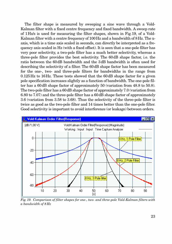
Fig. 29. 1st order of the radial, tangential and axial response, during a run-up of the spindrier, extracted using a three-pole Vold-Kalman filter with 50% bandwidth

The same peak value is found using one-pole and two-pole filters. For theone-pole filter with 38% bandwidth the extracted order is, however, contami-nated by ripples (beating interference), even at the resonance, due to thelimited selectivity. Fig. 29 shows the 1st order of the radial, tangential andaxial response extracted using a three-pole filter with a bandwidth of 50%.The same resonance is seen in the axial response, whereas the dominatingresonance in the tangential response is at 911RPM (15.2 Hz). A lower reso-nance at 375RPM (6.25 Hz) is seen in the radial and axial response and at388RPM (6.47 Hz) in the tangential response. T3 dB for this resonance isfound to be 415 ms for the radial response indicating that the bandwidthshould be at least 76%. Using 50% bandwidth with a three-pole filter givesan under-estimation of approximately 0.8 dB. A two-pole filter gives a beat-ing interference at this resonance with bandwidth larger than 50%, andproper measurement of this resonance is not possible with a one-pole filterdue to strong beating interference even for bandwidth as narrow as 20%.The 22nd order can be extracted using a three-pole filter with a bandwidthof 60%, which is found to be the minimum bandwidth for the dominating

36

resonance at 933RPM (15.6 Hz) in the radial response. A two-pole filter givesa small interference at the resonance with 60% bandwidth, and for a one-polefilter interference is experienced for bandwidths wider than 40%.

Crossing OrdersTo illustrate the effectiveness of the Vold-Kalman filter with decoupling ofclose and crossing orders, two signals have been mixed, a 1kHz signal and a300Hz to 2000Hz swept signal containing several orders as shown in theSTFT contour plot in Fig. 30. The duration of the signal is 6s. The examplesimulates a system with two independent axles. All orders and the 1kHz sinewave were generated with constant amplitude.

The first two swept orders and the 1kHz signal were extracted using 10%bandwidth (0.1 order resolution) two-pole Vold-Kalman filters without decou-pling. The magnitude of the two swept orders is shown in Fig. 31 and the 1kHzsignal is shown in Fig. 32. As seen in this case the 1kHz order strongly inter-acts with the swept 4th order around time 0.1s, the 3rd order around time 0.4s,

Fig. 30. An STFT of a signal mixed from a 1 kHz sine wave and a swept signal containingseveral harmonics (orders)

37

Fig. 31. First and second order of the swept signal extracted without decoupling usingtwo-pole Vold-Kalman filter with a bandwidth of 10%

Fig. 32. 1 kHz signal extracted without decoupling using two-pole Vold-Kalman filter witha bandwidth of 10%

38

39

Fig. 33. First and second order of the swept signal extracted using decoupling and two-pole Vold-Kalman filter with a bandwidth of 10%

Fig. 34. 1 kHz signal extracted using decoupling and two-pole Vold-Kalman filter with abandwidth of 10%

the 2nd order around time 1s and the first order around time 2.7s respec-tively, showing strong beating phenomena.

When the two tacho signals are used in a simultaneous estimation (i.e. withdecoupling), but with the same filter parameters as in the single order estima-tion (i.e. without decoupling), we achieve a dramatic improvement in the qual-ity of estimation, see Fig.33 and Fig.34. However, the 1kHz still interactswith the swept orders nos. 3 & 4, since they were not included in the calcula-tions.

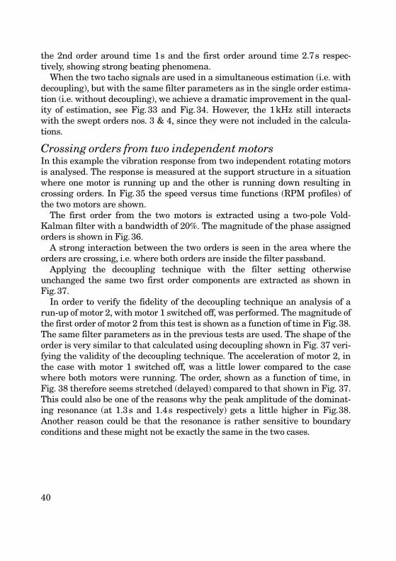
Crossing orders from two independent motorsIn this example the vibration response from two independent rotating motorsis analysed. The response is measured at the support structure in a situationwhere one motor is running up and the other is running down resulting incrossing orders. In Fig.35 the speed versus time functions (RPM profiles) ofthe two motors are shown.

The first order from the two motors is extracted using a two-pole Vold-Kalman filter with a bandwidth of 20%. The magnitude of the phase assignedorders is shown in Fig.36.

A strong interaction between the two orders is seen in the area where theorders are crossing, i.e. where both orders are inside the filter passband.

Applying the decoupling technique with the filter setting otherwiseunchanged the same two first order components are extracted as shown inFig.37.

In order to verify the fidelity of the decoupling technique an analysis of arun-up of motor 2, with motor 1 switched off, was performed. The magnitude ofthe first order of motor 2 from this test is shown as a function of time in Fig.38.The same filter parameters as in the previous tests are used. The shape of theorder is very similar to that calculated using decoupling shown in Fig. 37 veri-fying the validity of the decoupling technique. The acceleration of motor 2, inthe case with motor 1 switched off, was a little lower compared to the casewhere both motors were running. The order, shown as a function of time, inFig. 38 therefore seems stretched (delayed) compared to that shown in Fig. 37.This could also be one of the reasons why the peak amplitude of the dominat-ing resonance (at 1.3s and 1.4s respectively) gets a little higher in Fig.38.Another reason could be that the resonance is rather sensitive to boundaryconditions and these might not be exactly the same in the two cases.

40

Fig. 35. RPM as a function of time (speed profile) for motor 1 (green) and motor 2 (blue)

Fig. 36. First order of the two motors extracted using a two-pole Vold-Kalman filter with abandwidth of 20%. Notice the strong interaction (beating) between the two orders in thearea where the orders are crossing

41

Fig. 37. First order of the two motors extracted using decoupling. Vold-Kalman filter set-ting otherwise as in Fig.36 without the decoupling. Notice that the interaction (beating)between the orders is avoided

Fig. 38. First order in a run-up of motor 2 without motor 1 running. The Vold-Kalmanfilter parameters are the same as those used in Fig. 36 and Fig. 37. The result should becompared to that of motor 2 in Fig. 37 using decoupling

42

Sound Quality SynthesisSince the Vold-Kalman filter extracts order waveforms without time delay, i.e.,the extracted order time signals are coincident with the total signal; thesetime signals can be used for synthesis studies. This is especially interesting inthe field of Sound Quality Engineering, where time-, frequency- and order-editing and simulation of acoustic signals is an important tool for productsound optimisation. In the following simple example the Brüel&Kjær SoundQuality Software Type 7698 has been used for post-processing of Vold-Kalmandata. For sound perception the most dominating order is the 9th in the exam-ple shown in Figs.10–17. The 9th order waveform was subtracted (anyamount of attenuation is possible) from the total waveform using the mixerediting facility in version 3.0 of Type 7698 software. The time signal with the9th order removed is shown in Fig. 39, but a comparison with Fig.10 revealsno apparent visual difference, due to the fact that the amplitude of the 9thorder (see Fig.16) is about a factor of two smaller than the amplitude of thefirst order.

Fig. 39. Vibration time signal of the run-up with the 9th order removed (The amplitudescale changed to Pa)

43

Fig. 40. An STFT of the vibration signal with the 9th order removed

Fig. 41. Loudness analysis of the 9th order. Especially the frequency masking effect isclearly seen

44

45

It is on the other hand quite evident from the STFT contour plot shown inFig.40 compared to Fig.11, that the 9th order has been removed as well asthis was audible from a playback via the sound card of the original and editedsignals. Since Type 7698 is a dedicated package for sound measurement, theamplitude scaling is in SPL or Pa rms amplitudes rather than vibration levelsor vibration rms amplitudes. The SQ application provides the ability to listento both the extracted orders and to the residual sound with the ordersremoved.

The individual orders may be analysed using STFT, digital filtering (usingstandardised filter shapes such as 1/3-octaves), Loudness Analysis or othertechniques such as Wavelets or Wigner-Ville distribution [11, 21]. Fig.41shows an example where the 9th order waveform has been analysed usingnon-stationary Loudness calculations in order to study both time and fre-quency masking effects of the specific order.

Gearshift Example The measurement was done on a light truck with a V-8 engine and an over-drive automatic transmission, which was run on a dynamometer in a semi-anechoic room. Data was acquired using an eight-channel DAT recorder andshown here calibrated in volts, i.e. uncalibrated with respect to engineeringunits, such as Pa and m/s2. Using PULSE Interface to SONY DAT – Type7706 the digital data was interpolated and resampled and directly analyzedby PULSE via a SONY PCIF 500 SCSI interface box without any need for fur-ther digital/analogue/digital conversions. For this example a full-throttle run-up was performed under light load condition, using a tractive (drag) force ofonly 50 lbf (≈222 N). Fig.42 shows the RPM versus time curves from thetachometers on both the engine and the drive shaft (propeller shaft) for thecomplete run using a wide frequency and time range pre-analysis. See alsoRef. [3] for more details.

Microphone signals from a binaural recording using a Brüel&Kjær HATS(Head and Torso Simulator) Type 4100 in the passenger seat, as well as accel-erometer signals at several locations (pinion gear housing, transmission caseat drive shaft side etc.), were recorded. The right ear signal from the HATSwas analyzed in order to illustrate the capability of the Vold-Kalman OrderTracking Filter for handling gearshifts. It was decided to focus on the shiftfrom the 2nd gear into the 3rd gear around time 11,5 s shown in Fig.42. Thus asecond PULSE multi-analysis of the recording was performed using a Tachom-eter Analyzer for triggering and RPM detection and monitoring purposes, anFFT analyzer for real-time FFT-order processing and a Time Capture Ana-lyzer for capturing data for Vold-Kalman order tracking analysis.

Fig. 42. RPM profiles of run-up, with gear shift events

Fig. 43. Contour plot of Sound recording at right ear. Orders 4, 8 and 12, the engine firingharmonics are indicated

For the FFT analysis a 400 Hz baseband, 100 line analysis (T=250ms and∆f=4Hz) with Maximum overlap was performed. Maximum overlap was inthis case 99,5% since each FFT calculation including averaging etc. took1,4ms. Exponential averaging with 1 average was used. Spectra as well as pre-processed order slices were stored into a multi-buffer, using the 1900RPM of

46

the drive shaft as a start reference, i.e. used as time zero. Update interval was10 ms with a total of 551 spectra corresponding to a duration of 5,5s.

The Time Capture Analyzer was also triggered to start at 1900RPM makinga 5s recording up to approximately 2800RPM using a frequency range of1600Hz corresponding to a total of 20 480 time samples per channel.

Fig. 43 presents a contour plot of the microphone (time captured) signal fromthe right ear. 400 lines FFT with 80% overlap and a total of 96 spectra areshown. As expected the contour plot indicates that the dominant frequencycontent is found along the half-order lines of the engine, especially also atorders 4.0, 8.0 and 12.0, the V-8 engine firing harmonics. As seen the 4th orderis the dominating order both before and after the gearshift.

The data represents a typical case of high slew rates, especially the engineRPM at the shift points (up to 2800 RPM/s). Fig. 44 displays the engine RPMcurve near the shift from 2nd into 3rd gear, showing the curvefit RPM(smoothed) curve overlaid with the raw estimate (RPM table). The hinge pointwas found from the raw RPM by using the “display zoom” facility and visualinspection as well as the standard cursor readings, Maximum and MinimumValues (in this case found by PULSE at 1,758 s and at 2,280 s respectively).These numbers were then keyed into the Vold-Kalman RPM Curve Fit prop-erty page (see Fig.13). In the actual calculation the Number of Segments wasset to 10 even though fewer segments could have been used successfully.

Fig. 45 shows the magnitude of engine order 4.0, extracted using a three poleVold-Kalman filter with a relative bandwidth of 20% (≈10Hz). Fig. 46 showsthe magnitude of engine order 4.0 using real-time FFT processing. Also anorder slice bandwidth of 20% corresponding to approximately 2,5 FFT lineswas used for comparison purposes. Due to the record length of 250 ms, all FFTbased events are displaced, compared to the Vold-Kalman extracted order,with a delay of 125 ms corresponding to ½ the FFT record length.

When comparing the two 4th order slices the two methods agree extremelywell for the slowly changing amplitudes, but the FFT is not able to accuratelytrack the two rapid level changes which are seen in the Vold-Kalman resultsaround the shift point between time 2,0 s and 2,4 s. This is due to the fact thatthe Vold-Kalman filtering has no slew rate limitations although the real-timeFFT was actually able to track the RPM changes in this case. On the otherhand the Vold-Kalman filtering provides a better time resolution as well asmore data points compared to the FFT technique as explained in the following.

The FFT multi-buffer settings result in 501 data points along the 5s long Z-axis (25 multibuffer entries per FFT record-length, one entry per 7 FFT calcu-lations). Each FFT record represents approximately 94 ms (= 250ms × 37,5%)

47

Fig. 44. Detail of the Raw RPM (red colour) and the Curve Fit RPM (blue colour) at theshift point

Fig. 45. Engine order 4.0 extracted using Vold-Kalman order tracking filtering. X-axis isdisplayed from 0 s to 5s

when using a Hanning weighting function. The effective duration of the Han-ning weighting is defined in Ref. [5]. The Vold-Kalman technique results inthis case in 20480 data points (as mentioned earlier, for export purposes deci-mation of the data is possible). The selected frequency bandwidth of 10Hz cor-responds to a length of the IRF of 2τ = (0,2 × 2 / 10Hz) = 40ms.

48

Fig. 46. Engine order 4.0 extracted using real-time FFT processing. X-axis is displayedfrom 0,125 s to 5,125 s

In order to verify that the 4.0 order was extracted correctly, the order wave-form was subtracted from the original signal using the PULSE Sound Qualityapplication. A contour plot of the signal with the 4th order removed was suc-cessfully produced using a procedure as described earlier, see Figs.11 & 40.

In Ref. [3] also a file of the residual sound was generated by extracting the 14most significant engine orders, and then subtracting this file from the originalfile. This was done using the MTS* Systems Corporation IDEAS Sound Qual-ity software. The fact that this residual sound has consistently lower levels(about 30 dB) indicates that both the magnitude and phase of the extractedorders were processed with high fidelity, even passing through the gearshift.When listening to the residual sound produced by removing the Vold-Kalmanfiltered orders, only very little trace of the engine sound was heard through thegearshift. This fact is also a confirmation that the amplitude and phase track-ing is very accurate, and it also illustrates the practical value of the Vold-Kalman methods for harmonic extraction and editing in Sound Quality appli-cations involving high slew rates as found at gear shifts.

* AcknowledgementThe tape data was provided by courtesy of MTS Systems Corporation.

49

ConclusionThe Vold-Kalman filter enables order tracking without tracking-abilityslew rate limitations, with only speed limitation due to the filter responsetime. Phase assigned orders (shown as real, imaginary, magnitude, phase andNyquist plots) as well as order time waveforms (playback using sound cards)are available. Abrupt changes of the RPM, such as in gear shifts, and tachodrop-outs can be handled and finally decoupling of close and crossing orders ispossible. The only disadvantages of the technique is non-real time processing,“longer” calculation time, no information between orders and some priorknowledge of the contents of the signal is required.

The characteristics of the one-pole, two-pole and three-pole Vold-Kalmanorder tracking filters have been investigated in the time and the frequencydomain. The three-pole filter has the best selectivity and therefore the bestability to suppress ripples due to beating interference from the other ordercomponents in the signal. In the time response to a tone burst the two- andthree-pole filters exhibit small ripples (overshoot). This will, however, onlycontaminate the results when the signal contains abrupt changes in theamplitude or when the bandwidth of the filter is selected too narrow for thesignal.

The time-frequency relationship of the three filter types shows an optimumrelationship close to the Heisenberg’s uncertainty limit and is given by B3dB × τ= 0.2, where B3dB is the 3dB bandwidth of the Vold-Kalman filter and τ is thetime it takes for the time response to decay 8.69dB (a factor of e).

Selection of the bandwidth of the filter should follow B3dB ≥ 2 /T3dB, whereT3dB is the time it takes for an order to sweep through the 3dB bandwidth of aresonance (or the time it takes for an order to change 6dB in amplitude). Inalmost all cases the three-pole filter is the best choice due to its better selectiv-ity in the frequency domain. Today the main use of single pole filter is to beable to duplicate processing done in earlier implementation of the Vold-Kalman filtering.

In situations where different orders related to different rotating shafts(tacho signals) are close or crossing each other, decoupling can be used to sepa-rate the orders without beating interference.

50

References1) Vold, H., Leuridan, J., “Order Tracking at Extreme Slew Rates, Using

Kalman Tracking Filters”, SAE Paper Number 931288, 1993 2) Vold, H., Mains, M., Blough, J., “Theoretical Foundations for High Per-

formance Order Tracking with the Vold-Kalman Tracking Filter”, SAEPaper Number 972007, 1997

3) Vold, H., Deel, J., “Vold-Kalman Order Tracking: New Methods for Vehi-cle Sound Quality and Drive Train NVH Applications”, SAE PaperNumber 972033, 1997

4) Brüel&Kjær, “PULSE, the Multi-Analyzer System - Type 3560”, Prod-uct Data, BP 1611-14, BP1795

5) Gade, S., Herlufsen, H., Konstantin-Hansen, H., Wismer, N.J., “OrderTracking Analysis”, Technical Review No.2, 1995, Brüel&Kjær

6) Blough, J., Brown, D., Vold, H., “The Time Variant Discrete FourierTransform as an Order Tracking Method”, SAE Paper Number 972006,1997

7) Vold, H., Kundrat, J., Rocklin, G., Russell, R., “A Multi-Input ModalEstimation Method for Mini-Computers”, SAE Paper Number 820194,1982

8) Kalman, R. E., “A new approach to linear filtering and prediction prob-lems”, Trans. Amer. Soc. Mech. Eng., J. Basic Engineering, 82, 32–45,1960

9) Kalman, R. E., Bucy, R. S., “New results in linear filtering and predictiontheory”, Trans. Amer. Soc. Mech. Eng., J. Basic Engineering, 83, 95–108, 1961

10) Vold, Herlufsen, Mains, Corwin-Renner, “Multiple Axle Order Trackingwith the Vold-Kalman Tracking Filter”, Sound and Vibration Magazine,30–34, May 1997

11) Leuridan, J., Van der Auweraer, H., Vold, H., “The Analysis of Nonsta-tionary Dynamic Signals”, Sound & Vibration Magazine, 14–26,August 1994

12) Randall, R.B., “Frequency Analysis”, Brüel&Kjær, 198713) Brigham, E.O., “The Fast Fourier Transform”, Prentice-Hall, Inc.,Engle-

wood Cliffs, N.J., 197414) Gade S., Herlufsen. H., Konstantin-Hansen, H., Ladegaard, P., “Simul-

taneous Zwicker Loudness and One Third Octave Measurements”, Inter-noise Proceedings, Christchurch, NZ, 1998

15) Gade S., Herlufsen. H., “Use of weighting Functions in DFT/FFT Anal-ysis”, Brüel&Kjær Technical Reviews Nos. 3 & 4, 1987

51

16) Brüel& Kjær, “Vold-Kalman Order Tracking Filter – Type 7703”, Prod-uct Data, BP 1760

17) Brüel&Kjær, “Time Capture – Type 7705”, Product Data, BP 176218) Brüel&Kjær, “Order Analysis – Type 7702”, Product Data, BP 163419) Gade S., Herlufsen. H., “Digital Filter Techniques vs. FFT Techniques

for Damping Measurement”, Brüel&Kjær Technical Review No. 1, 199420) Leuridan, J., Kopp, G.E., Moshrefi, N., Vold, H., “High Resolution Order

Tracking Using Kalman Tracking Filters – Theory and Applications”,SAE Paper Number 951332, 1995

21) Gade, S., Gram-Hansen, K., “Non-stationary Signal Analysis usingWavelet Transform, Short-time Fourier Transform and Wigner-Ville Dis-tribution”, Brüel&Kjær Technical Review Nos. 2, 1996

52

Appendix AWe have observed that all time response curves are crossing at −6 dB at thetwo points in time where the applied tone burst is started and where it is dis-continued, Figs. 21 & 22. At theses points in time we have that ½ the filtertime response contains the signal while the rest of the filter time responsecontains no signal. Thus the overall time response has decayed by 3dB (halfpower) while the signal inside the tracking filter has decayed by 6dB. A simi-lar phenomena is observed using FFT analysis and is explained in details inthe following.

As an illustration, an FFT analysis using 400 lines, frequency range of fspan= 1600Hz, resolution of ∆f = 4Hz and a record length of 250ms is used. A sinu-soidal signal of 1Vrms, 800Hz (i.e., 200 periods) is analyzed as shown in Fig.A1.Cursor readings show in Fig.A2 the level to be 0dB at 800Hz as well as thetotal power is 0dB. No leakage is seen.

Fig. A1. Time signal of a 1Vrms, 200 period, 800 Hz sine wave analyzed using a rectangu-lar weighting function

53

Fig. A2. Frequency spectrum of a 200 period, 800 Hz sine wave analyzed using a rectangu-lar weighting function, no leakage is seen

Using a rectangular weighting with an amplitude of A and time length of Tresults in a spectrum weighting of

H(f) = AT × sin(πTf) / (πf ) (A1)

which is convolved with the spectrum of the 800Hz signal and then sampled(in this case) at frequencies which is multiples of ∆f = 4Hz. The weightingfunction and its corresponding spectrum are shown in Fig.A3. A main lobewith a maximum amplitude of AT and a width of 2∆f is shown, and all sidelobes have a width of ∆f. In this case the spectrum is sampled at the centre ofthe main lobe and at all zero crossings between the lobes resulting in a calcu-lated/displayed FFT spectrum consisting of one line only, which is scaled to anamplitude value of 1 corresponding to 0dB. See Ref. 12 (Appendix A) and Ref.13 (Chapter 2).

54

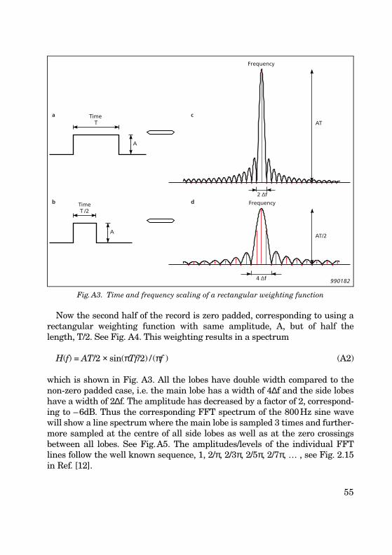
Fig. A3. Time and frequency scaling of a rectangular weighting function

Now the second half of the record is zero padded, corresponding to using arectangular weighting function with same amplitude, A, but of half thelength, T/2. See Fig. A4. This weighting results in a spectrum

H(f) = AT/2 × sin(πTf/2) / (πf ) (A2)

which is shown in Fig. A3. All the lobes have double width compared to thenon-zero padded case, i.e. the main lobe has a width of 4∆f and the side lobeshave a width of 2∆f. The amplitude has decreased by a factor of 2, correspond-ing to –6dB. Thus the corresponding FFT spectrum of the 800Hz sine wavewill show a line spectrum where the main lobe is sampled 3 times and further-more sampled at the centre of all side lobes as well as at the zero crossingsbetween all lobes. See Fig.A5. The amplitudes/levels of the individual FFTlines follow the well known sequence, 1, 2/π, 2/3π, 2/5π, 2/7π, … , see Fig. 2.15in Ref. [12].

9901824 ∆f

2 ∆f

Frequency

Frequency

ATTa Time

Timeb

c

d

A

AT/2

T /2

A

55

Fig. A4. Time signal of a 200 period, 800 Hz sine wave analyzed using half a rectangularweighting function, i.e. only 100 periods are within the window

Fig. A5. Frequency spectrum of a 200 period, 800 Hz sine wave analyzed using half a rec-tangular weighting function, i.e. only 100 periods are within the window

56

The cursor readings show a level of –6dB at 800Hz as expected according tothe discussion above. The total level is –3dB (half power), which is alsoexpected since the time window contains data in only half the record in thiscase.

This is also the case using other time weighting functions as long as they aresymmetrical in time. Figs. A6 & A7 show the results using Hanning weighting.

In this case the resulting spectrum is most easily understood by convolvingthe FFT spectrum shown in Fig. A5, with the FFT spectrum of a Hanningweighting function, taking amplitude as well as phase into account. Thephase of the spectrum shown in Fig. A5 is +90 degrees for all non-zero ampli-tude values at frequencies lower than the centre frequency, 0 degrees at thecentre frequency and –90 degrees for all non-zero amplitude values at fre-quencies higher than the centre frequency, see Fig. 2.24 Ref. [12]. The Fourierspectrum of a Hanning (scaled to an amplitude of 2 in the centre of the record)consists of three values, 1 at the centre frequency, f0 and –½ (or ½ and a phaseof 180o) at the two neighbouring frequencies, f0 – ∆f and f0 + ∆f. From themean square values the Noise Bandwidth of the Hanning weighting is foundto be 12 + ½2 + ½2 = 1.5 or 1.76dB. See ref. [15].

Fig. A6. Time signal of a 200 period, 800 Hz sine wave analyzed using half a Hanningweighting function, i.e. only 100 periods are within the window

57

Fig. A7. Frequency spectrum of a 200 period, 800 Hz sine wave analyzed using half a Han-ning weighting function, i.e. only 100 periods are within the window

Convolution of the spectrum in Fig. A5 with the spectrum of a Hanningresults in the spectrum shown in Fig. A7 as explained in the following.

When one of the zero values are convolved with the Hanning the result is anamplitude value which is the mean value of the two adjacent lines but withopposite phase.

When one of the non-zero side lobe values are convolved with the spectrumof a Hanning, the original value is unchanged due to the fact that the two adja-cent lines have zero amplitude values.

When the centre frequency value at f0 is convolved with the spectrum of aHanning the original is unchanged due to the fact that the two adjacent lineshave equal amplitude but opposite phase.

To convolve the two lines adjacent to the centre frequency with the spectrumof the Hanning requires a little more complex calculation, resulting in a slightincrease in amplitude from 0.32 (–9.9dB) to 0.40 (–7.9dB) and a phase changefrom respectively 90° to 128° for the left, (f0 – ∆f) and –90° to –128° for theright, (f0 – ∆f) FFT line.

Thus for the resulting spectrum shown in Fig. A7 the centre line will also inthis case show a level of –6dB and the total power of the spectrum –3dB, after

58

compensating the total reading for the Noise Bandwidth (1.76dB) of the Han-ning weighting.

ConclusionWhen the FFT time record contains a stationary sinusoidal signal in only thefirst or the last half of the record the total power of the spectrum is decreasedby 3dB irrespective of choice of weighting function as long as this function issymmetrical in the record. Half of the power/energy of this signal (–6dB) isfound at the expected frequency while the rest (–6dB) is found as leakage.Using a Vold-Kalman order tracking filter, which also has a symmetrical timeresponse, the leakage components are normally not seen, while the –6dB levelof the tracking frequency is observed in the time response as discussed aboveas well as shown in Fig. 22.

59

Previously issued numbers ofBrüel & Kjær Technical Review(Continued from cover page 2)

4–1986 Field Measurements of Sound Insulation with a Battery-Operated

Intensity AnalyzerPressure Microphones for Intensity Measurements with Significantly Improved Phase PropertiesMeasurement of Acoustical Distance between Intensity Probe MicrophonesWind and Turbulence Noise of Turbulence Screen, Nose Cone and Sound Intensity Probe with Wind Screen

3–1986 A Method of Determining the Modal Frequencies of Structures with Coupled ModesImprovement to Monoreference Modal Data by Adding an Oblique Degree of Freedom for the Reference

2–1986 Quality in Spectral Match of Photometric TransducersGuide to Lighting of Urban Areas

1–1986 Environmental Noise Measurements4–1985 Validity of Intensity Measurements in Partially Diffuse Sound Field

Influence of Tripods and Microphone Clips on the Frequency Response of Microphones

3–1985 The Modulation Transfer Function in Room AcousticsRASTI: A Tool for Evaluating Auditoria

2–1985 Heat StressA New Thermal Anemometer Probe for Indoor Air Velocity Measurements

1–1985 Local Thermal Discomfort

Special technical literatureBrüel&Kjær publishes a variety of technical literature which can be obtained from your local Brüel&Kjær representative.The following literature is presently available:

❍ Acoustic Noise Measurements (English), 5th. Edition❍ Noise Control (English, French)❍ Frequency Analysis (English), 3rd. Edition❍ Catalogues (several languages)❍ Product Data Sheets (English, German, French,)

Furthermore, back copies of the Technical Review can be supplied as shown in the list above. Older issues may be obtained provided they are still in stock.

TECHNICAL REVIEWCharacteristics of the Vold-Kalman Order Tracking Filter

1999

HEADQUARTERS: DK-2850 Nærum · DenmarkTelephone: +45 45 80 05 00 · Fax: +45 45 80 14 05Internet: http://www.bk.dk · e-mail: info@bk.dk

BV

0052

–11

ISSN

000

7–26

21

BV0052-11_omslag.qxd 10/02/00 13:53 Page 1