
Technical Report Title Authors - Robotics Institute · scheduling of stopping trajectories. Safety...
33
Technical Report Title Fast Exploration Using Multirotors: Analysis, Planning, and Experimentation Authors Kshitij Goel Micah Corah Nathan Michael CMU-RI-TR-19-03 The Robotics Institute Carnegie Mellon University Pittsburgh, Pennsylvania 15213 February 2019 Copyright © 2019 Kshitij Goel, Micah Corah, Nathan Michael
Transcript of Technical Report Title Authors - Robotics Institute · scheduling of stopping trajectories. Safety...
Technical Report
Title
Fast Exploration Using Multirotors: Analysis, Planning, and Experimentation
Authors
Kshitij Goel
Micah Corah
Nathan Michael
CMU-RI-TR-19-03
The Robotics Institute
Carnegie Mellon University
Pittsburgh, Pennsylvania 15213
February 2019
Copyright © 2019
Kshitij Goel, Micah Corah, Nathan Michael

Abstract
High speed flight with multirotor aerial vehicles is limited by constraints on size, sensing
range, on-board computation, accelerations, and velocities. For robotic exploration and
operation in unknown environments, guaranteeing collision-free operation and selecting in-
formative sensing actions further increase complexity. To this end, this work presents three
contributions. First, we analyze the rate of reduction of the entropy of the map for idealized
scenarios considering constraints on dynamics and sensing for a multirotor vehicle. Second,
we propose an action representation that accounts for platform dynamics and provides ac-
tions that are useful for rapid exploration based on the prior analysis. Third, we present
a receding-horizon sampling-based planner that uses this action representation, maximizes
information gain, and ensures safe operation at high speeds. Finally, we present extensive
simulation experiments in a complex 3D environment that demonstrate the significance of
action design, horizon length, and replanning rate on exploration performance.
2
Contents
1 Introduction 7
2 Idealized Exploration Analysis 9
2.1 Problem Description . . . . . . . . . . . . . . . . . . . . . . . . . . . . . . . 9
2.2 System Model and Safety Constraints . . . . . . . . . . . . . . . . . . . . . . 10
2.3 Exploration Scenarios . . . . . . . . . . . . . . . . . . . . . . . . . . . . . . . 11
2.3.1 Perpendicular to frontier . . . . . . . . . . . . . . . . . . . . . . . . . 11
2.3.2 Parallel to frontier . . . . . . . . . . . . . . . . . . . . . . . . . . . . 12
2.4 Bounds on Velocity . . . . . . . . . . . . . . . . . . . . . . . . . . . . . . . . 12
2.5 Bounds on Rate of Exploration . . . . . . . . . . . . . . . . . . . . . . . . . 13
2.5.1 Perpendicular to frontier . . . . . . . . . . . . . . . . . . . . . . . . . 13
2.5.2 Parallel to frontier . . . . . . . . . . . . . . . . . . . . . . . . . . . . 14
3 Action Representation 15
3.1 Motion Primitive Library Generation . . . . . . . . . . . . . . . . . . . . . . 15
3.2 Action Space for Fast Exploration . . . . . . . . . . . . . . . . . . . . . . . . 16
3.3 Minimum Feasible Duration Search . . . . . . . . . . . . . . . . . . . . . . . 17
4 Action Selection 19
4.1 Information-Theoretic Exploration Objectives . . . . . . . . . . . . . . . . . 19
4.2 Monte Carlo Tree Search (MCTS) . . . . . . . . . . . . . . . . . . . . . . . . 20
4.3 Safety at High Speeds . . . . . . . . . . . . . . . . . . . . . . . . . . . . . . 21
4.4 Scheduling Planner Output . . . . . . . . . . . . . . . . . . . . . . . . . . . 22
5 Results 24
5.1 Simulation Experimentation Setup . . . . . . . . . . . . . . . . . . . . . . . 25
5.1.1 Inertial and Sensing Parameters . . . . . . . . . . . . . . . . . . . . . 25
5.1.2 Triggered Simulation . . . . . . . . . . . . . . . . . . . . . . . . . . . 26
5.2 Effects of Action Design . . . . . . . . . . . . . . . . . . . . . . . . . . . . . 26
5.3 Effects of Planning Rate . . . . . . . . . . . . . . . . . . . . . . . . . . . . . 29
5.4 Effects of Finite-Horizon Length . . . . . . . . . . . . . . . . . . . . . . . . . 30
6 Conclusion 31
6.1 Contributions . . . . . . . . . . . . . . . . . . . . . . . . . . . . . . . . . . . 31
6.2 Limitations & Future Work . . . . . . . . . . . . . . . . . . . . . . . . . . . 31

List of Figures
1 A multirotor explores a complex unstructured three-dimensional environment
(occupied voxels in black) using the proposed planning approach. In this
work, we first present analysis for bounds on exploration performance in ideal
scenarios taking model constraints into account. Secondly, we propose a finite-
horizon planning approach that leverages this analysis and ensures safety at
high speeds. Last, we conduct extensive simulation experiments and draw
conclusions on various factors affecting exploration performance. . . . . . . . 8
2 An ideal multirotor exploration scenario with no obstacles in the environment.
The objective is to design a planner that takes actions such that over time, all
of the unknown space (black voxels) is explored (white voxels) using a time-
of-flight sensor while ensuring that the robot motion and planned trajectories
are always within the free space (white voxels). . . . . . . . . . . . . . . . . 9
3 Ideal exploration scenarios considered for exploration performance analysis in
Sect. 2. Upper bounds on rate of novel voxels explored are computed for a
double integrator system moving towards sensor scan (V⊥,max) and parallel
to it (V‖,max) while performing rapid yaw motion. Environment is assumed
completely free (Xunk = Xfree) while sensor scan is delayed by ∆tm. . . . . . . 10
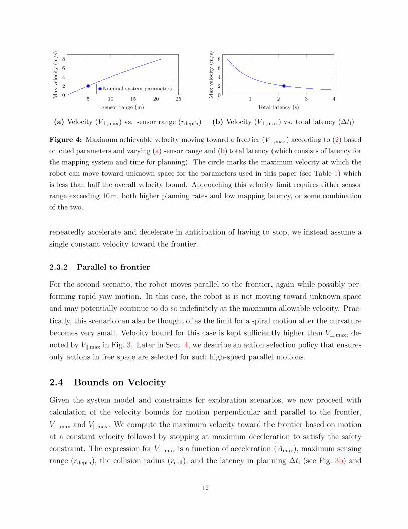
4 Maximum achievable velocity moving toward a frontier (V⊥,max) according to
(2) based on cited parameters and varying (a) sensor range and (b) total
latency (which consists of latency for the mapping system and time for plan-
ning). The circle marks the maximum velocity at which the robot can move
toward unknown space for the parameters used in this paper (see Table 1)
which is less than half the overall velocity bound. Approaching this velocity
limit requires either sensor range exceeding 10 m, both higher planning rates
and low mapping latency, or some combination of the two. . . . . . . . . . . 12
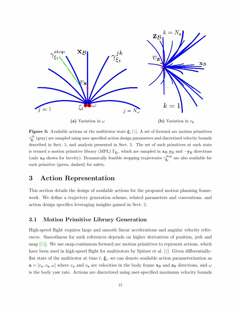
5 Available actions at the multirotor state ξt [1]. A set of forward arc motion
primitives γjkξt (gray) are sampled using user specified action design parameters
and discretized velocity bounds described in Sect. 3, and analysis presented in
Sect. 2. The set of such primitives at each state is termed a motion primitive
library (MPL) Γξt , which are sampled in xB,yB and −yB directions (only xB
shown for brevity). Dynamically feasible stopping trajectories γstopξtare also
available for each primitive (green, dashed) for safety. . . . . . . . . . . . . 15
4

6 Brief overview of the general Monte Carlo tree search (MCTS) algorithm [2, 3].
Planner selects the deepest node that has unexpanded children based on the
selection policy, which is usually based on Upper Confidence Bounds (UCB).
From this selected node, children are expanded according to a random rollout
policy until a terminal state or condition is reached. The cumulative reward
and node visit statistics during this rollout are stored and back-propagated
along the path to the root state. This process is iterated until a user-specified
computational budget is reached, and the sequence of actions with the best
rewards to visits ratio is returned. . . . . . . . . . . . . . . . . . . . . . . . . 19
7 Overview of safe node expansion in the proposed MCTS-planner and the
scheduling of stopping trajectories. Safety checks detailed in Alg. 3 and
Sect. 4.3 ensure that all trajectory segments (a), (b), and (c) lie in free space,
Xfree. Segment (a) is scheduled at root node ξ0, while segments (b) and (c) are
scheduled at the end of the current planning round ξp. One of the segments
(b) or (c) are selected for tracking at ξp based on the output of the next plan-
ning round. This approach to scheduling and safety checking ensures that the
vehicle is always able to stop within Xfree, even there is a failure in finding a
feasible action during a one of the planning rounds. . . . . . . . . . . . . . . 23
8 Different stages of exploration with respect to time for three-dimensional un-
structured environment considered for evaluation of the proposed motion plan-
ning framework. Black voxels denote space marked as occupied. We consider
a large room in 3D warehouse environment with dimensions 60 m×30 m×11 m. 24
9 Rate of exploration variations with time to investigate effects of changes in ac-
tion design on exploration performance. We observe substantial improvement
in performance due to availability of parallel motions (a, c), while perfor-
mance increment due to high speed perpendicular actions is observed to be
minimal (b, d). . . . . . . . . . . . . . . . . . . . . . . . . . . . . . . . . . . 27
10 Results for effects of planning rate on exploration performance in a three-
dimensional scenario. Two metrics, entropy reduction rate (a) and entropy
reduction (b), are shown with respect to time. We observe a peculiar behavior
– entropy reduction rate maximizes for 1 Hz planning rate, performing better
than 2 Hz and 5 Hz. Furthermore, a substantial part of the environment is left
unexplored at 0.5 Hz (b). . . . . . . . . . . . . . . . . . . . . . . . . . . . . . 29
5

11 Variation in length of the finite-horizon and its effects on exploration perfor-
mance in a two-dimensional scenario. Two metrics, entropy reduction rate
(a) and entropy reduction (b), are shown with respect to time. As expected,
longer finite horizon results in significantly better exploration rate (here we
compare 2 second with a 4 second horizon). . . . . . . . . . . . . . . . . . . 30
List of Tables
1 Ideal upper bounds on velocity and rate of entropy reduction for two ideal
scenarios described in Sect. 2. All values are computed for a planning rate of
1 Hz, mapping latency 0.2 s, sensor point cloud of size 4.0 m × 3.15 m, occu-
pancy grid resolution of 20 cm, overall bound on top speed Vmax at 8 m/s, and
collision radius rcoll set at 0.3 m. . . . . . . . . . . . . . . . . . . . . . . . . . 13
2 Discretization used to construct action space Xact using ideal analysis pre-
sented in Sect. 2. We compute velocity bounds for the planning rate of 1 Hz,
i.e. V⊥,max = 2.04 m/s and V‖,max = 8 m/s. For all action sets, maximum yaw
rate is 1.0 rad/s and maximum vertical vz is kept at 1.5 m/s. Total number of
primitives for a MPL are denoted by Nprim = Nω ·Nz. . . . . . . . . . . . . . 17
3 Inertial properties and dynamics constraints for the multirotor used in the
simulation experiments. . . . . . . . . . . . . . . . . . . . . . . . . . . . . . 25
4 Sensing constraints for the forward facing depth camera used in for the explo-
ration experiments. . . . . . . . . . . . . . . . . . . . . . . . . . . . . . . . . 25
5 Average rates at which various types of high and low speed primitives are
selected by the action selector. These rates are calculated after averaging
number of primitives selected of the said type with respect to the total number
of planning rounds across trials. . . . . . . . . . . . . . . . . . . . . . . . . . 26
6
1 Introduction
Fast and safe motion planning policies for unknown environments can be useful when robots
operate in challenging scenarios such as urban search-and-rescue and disaster response. In
such scenarios, it is essential for a robot or a team of robots to find survivors or specific objects
in an unstructured and unknown three-dimensional environment rapidly while maintaining
collision-free operation. Aerial robots equipped with time-of-flight sensors have been used
previously in a three-dimensional exploration context and have been shown to be useful
in such hazardous scenarios [4, 5]. However, such platforms are often size, weight, and
power (SWaP) constrained which places bounds on available actions during flight as well as
limiting the choice of sensing modalities. At the same time, SWaP constraints also place
bounds on the dynamics such as the maximum acceleration that the robot can achieve in
flight. Rapid exploration using such constrained multirotors thus requires motion planning
frameworks that enable safe navigation in unknown environments while accounting for model
constraints and decreasing the uncertainty of the map [6].
Previous works have begun to consider the effects of platform dynamics on high speed
exploration and navigation in unknown environments. Cieslewski et al. [6] take into account
aerodynamic effects and sensing limits to place bounds on permissible velocities towards
frontiers. While these upper bounds ensure that the multirotor can safely come to a halt
within the maximum sensor range, the velocity bounds also depend on how fast the frontier
locations are updated, i.e., the planning rate. Liu et al. [7] address this by accounting
for time delay in processing sensor data in addition to model constraints to generate safe
stopping trajectories for each planning iteration. However, an analysis on how planning
rates and model constraints affect velocity bounds and exploration performance is lacking
in the literature. In this work, we account for planning rates using a similar approach as
Liu et al. [7] and provide analysis using a simplified quadrotor model to identify limits on
exploration performance given model constraints. This analysis is later used to design an
action representation as part of a proposed motion planning framework for rapid exploration.
Intuitively, information reward is high when the robot moves towards a frontier [6, 8].
Cieslewski et al. [6] pose exploration as a frontier selection problem and suggest selection
of frontiers that lie in the direction of the flight path and adapt the velocity based on the
sensor range and aerodynamic considerations. Although this approach provides insight into
maintaining safety during rapid exploration, the motivation for the approach is incomplete
as a more broad variety of actions such as yawing motions and motions parallel to a frontier
can provide improved performance for rapid exploration. In the first part of this work, we
7

Figure 1: A multirotor explores a complex unstructured three-dimensional environment (occupied
voxels in black) using the proposed planning approach. In this work, we first present analysis
for bounds on exploration performance in ideal scenarios taking model constraints into account.
Secondly, we propose a finite-horizon planning approach that leverages this analysis and ensures
safety at high speeds. Last, we conduct extensive simulation experiments and draw conclusions on
various factors affecting exploration performance.
address bounds on both linear and yaw rates and analyze rates of exploration given dynamics
and sensing constraints. Specifically, given a constrained aerial platform, upper bounds
on these velocities and rate of entropy reduction are derived for an idealized exploration
scenario. Using these upper bounds, we propose a information-theoretic motion planning
framework for high speed exploration that accounts for velocity and acceleration bounds
in both action representation and selection. Lastly, we conduct simulation experiments
in a large unstructured three-dimensional warehouse environment and analyze affects on
exploration performance to show the significance of action design, finite-horizon length, and
replanning rates.
This report proceeds as follows. Sect. 2 presents an idealized analysis on exploration per-
formance bounds given platform constraints. Action representation for the proposed motion
planning framework is developed in Sect. 3 followed by action selection policy description in
Sect. 4. Sect. 5 details experimental results, with concluding remarks presented in Sect. 6.
8

Figure 2: An ideal multirotor exploration scenario with no obstacles in the environment. The
objective is to design a planner that takes actions such that over time, all of the unknown space
(black voxels) is explored (white voxels) using a time-of-flight sensor while ensuring that the robot
motion and planned trajectories are always within the free space (white voxels).
2 Idealized Exploration Analysis
The goal of this section is to investigate bounds on exploration performance for a constrained
multirotor platform. We impose constraints based on dynamics, depth sensing, and compute
bounds on the rate of entropy reduction for nominal conditions. We start with defining the
exploration problem in Sect. 2.1, model simplifications and safety constraints in Sect. 2.2,
followed by description of ideal exploration scenarios in Sect. 2.3. Bounds of velocity and
exploration rate are calculated in Sect. 2.4 and Sect. 2.5 respectively. Later, in Sect. 3, we
leverage these insights on velocities and exploration rates to design actions for the proposed
motion planning strategy for exploration.
2.1 Problem Description
Figure 2 depicts a typical multirotor exploration scenario. Environment is modeled by an
occupancy grid map with independent Bernoulli occupancy probabilities for voxels with a
side-length c. Depending on user-specified thresholds for occupancy, the map is partitioned
into three subsets: free space (Xfree, white voxels in Fig. 2), unknown space (Xunk, black voxels
9

(a) Ideal exploration scenarios (b) Sensor top view (c) Sensor perspective view
Figure 3: Ideal exploration scenarios considered for exploration performance analysis in Sect. 2.
Upper bounds on rate of novel voxels explored are computed for a double integrator system mov-
ing towards sensor scan (V⊥,max) and parallel to it (V‖,max) while performing rapid yaw motion.
Environment is assumed completely free (Xunk = Xfree) while sensor scan is delayed by ∆tm.
in Fig. 2), and occupied space (Xocc). The voxels at the boundary of Xfree and adjacent to
voxels in Xunk are called frontier voxels, denoted by the set Xfrt [8]. The objective of a motion
planner in such exploration scenarios is to maximize the rate at which the amount of free
space, Xfree, is explored. This rate is quantified as the rate of reduction of entropy of the
occupancy map [9]. The entropy of the map decreases as the occupancy values of previously
unknown voxels are updated based on sensor observations and become more certain, and
there is at most one bit of entropy per voxel. Hence, we reason about the rate of reduction
in entropy using bounds on the number of novel voxels covered per unit time.
Furthermore, the planned trajectories and the robot should always lie within the safe
space Xfree to ensure safety. This constraint, along with constraints specific to the multirotor
platform, limit the minimum time in which an area can be explored. In this ideal analysis,
we investigate what are these limits in ideal exploration scenarios and how can these limits
inform the design of our proposed motion planner.
2.2 System Model and Safety Constraints
This work applies a simplified double-integrator quadrotor model with acceleration and ve-
locity constraints for analysis of limits on exploration performance. Such a model can be
thought of as a relaxation of dynamics models that are commonly used for position and atti-
tude control of multirotor vehicles [10, 11]. Denote the position of the vehicle as r = [x, y, z]T
in an inertial world frame W = xW ,yW , zW and the yaw as ψ, assuming small roll and
pitch angles. Given the yaw angle, we denote the state as ξ = [rT, ψ, rT, ψ]T and the body
10

frame as B = xB,yB, zB. The derivatives of position and yaw satisfy
||r||2 ≤ Vmax ||r||2 ≤ Amax |ψ| ≤ Ωmax (1)
where || · ||2 is the 2-norm.
For the purpose of this analysis, we are interested in computing ideal upper bounds on
rate of novel voxels observed by the multirotor. In an ideal exploration scenario (Fig. 3a),
unknown voxels are all unoccupied, and the robot is able to explore rapidly subject only to
constraints on dynamics and safety.
However, the requirement for collision-free operation constrains the set of actions that a
multirotor can safely execute while navigating in an unknown environments. In this case,
the environment is incrementally revealed to the multirotor via measurements obtained from
a depth sensor facing in the xB direction, which has a maximum range of rdepth (Fig. 3a, 3b).
A planning policy can ensure collision-free operation by guaranteeing that the robot is able
to stop within Xfree—given an appropriate collision radius rcoll (Fig. 3b)—such as in the work
of Janson et al. [12]. In the worst case, any voxel in Xunk may be revealed to be occupied
and so possibly force the robot to stop within Xfree from any state ξt at time t. We define
exploration scenarios and such velocity bounds later in Sect. 2.3.
Plans are generated every ∆tp seconds, and, additionally, we assume bounded latency
for acquiring depth information and integrating it into the occupancy map, denoted by ∆tm
(Fig. 3b). As such, the action being executed at any given time is based on sensor data
that is no older than ∆tl = 2∆tp + ∆tm. The first planning duration accounts for planning
computation, based on data that is at most ∆tm old. The second accounts for execution of
the planned action while the robot re-plans again.
2.3 Exploration Scenarios
We now define the two basic steady-state exploration scenarios that we consider in this
analysis.
2.3.1 Perpendicular to frontier
In this scenario, the robot moves toward the frontier, in the direction of the unknown space,
possibly while performing a rapid yaw motion. As discussed in Sect. 2.2, the robot must
be able to stop before entering the unknown space which places an upper bound, denoted
by V⊥,max in Fig. 3a and Fig. 3b. For this analysis, rather than allowing for the robot to
11
5 10 15 20 250
2
4
6
8
Sensor range (m)
Maxvelocity
(m/s)
Nominal system parameters
(a) Velocity (V⊥,max) vs. sensor range (rdepth)
1 2 3 40
2
4
6
8
Total latency (s)
Maxvelocity
(m/s)
(b) Velocity (V⊥,max) vs. total latency (∆tl)
Figure 4: Maximum achievable velocity moving toward a frontier (V⊥,max) according to (2) based
on cited parameters and varying (a) sensor range and (b) total latency (which consists of latency for
the mapping system and time for planning). The circle marks the maximum velocity at which the
robot can move toward unknown space for the parameters used in this paper (see Table 1) which
is less than half the overall velocity bound. Approaching this velocity limit requires either sensor
range exceeding 10 m, both higher planning rates and low mapping latency, or some combination
of the two.
repeatedly accelerate and decelerate in anticipation of having to stop, we instead assume a
single constant velocity toward the frontier.
2.3.2 Parallel to frontier
For the second scenario, the robot moves parallel to the frontier, again while possibly per-
forming rapid yaw motion. In this case, the robot is is not moving toward unknown space
and may potentially continue to do so indefinitely at the maximum allowable velocity. Prac-
tically, this scenario can also be thought of as the limit for a spiral motion after the curvature
becomes very small. Velocity bound for this case is kept sufficiently higher than V⊥,max, de-
noted by V‖,max in Fig. 3. Later in Sect. 4, we describe an action selection policy that ensures
only actions in free space are selected for such high-speed parallel motions.
2.4 Bounds on Velocity
Given the system model and constraints for exploration scenarios, we now proceed with
calculation of the velocity bounds for motion perpendicular and parallel to the frontier,
V⊥,max and V‖,max. We compute the maximum velocity toward the frontier based on motion
at a constant velocity followed by stopping at maximum deceleration to satisfy the safety
constraint. The expression for V⊥,max is a function of acceleration (Amax), maximum sensing
range (rdepth), the collision radius (rcoll), and the latency in planning ∆tl (see Fig. 3b) and
12

Table 1: Ideal upper bounds on velocity and rate of entropy reduction for two ideal scenarios
described in Sect. 2. All values are computed for a planning rate of 1 Hz, mapping latency 0.2 s,
sensor point cloud of size 4.0 m× 3.15 m, occupancy grid resolution of 20 cm, overall bound on top
speed Vmax at 8 m/s, and collision radius rcoll set at 0.3 m.
Value/CasesArea
(m2)
Velocity
(m/s)
Entropy rate
(bits/s)
Perpendicular (⊥) 12.60 2.04 3.21× 10³
Parallel (‖) 19.00 8.00 1.90× 10⁴
⊥, rapid yaw 31.50 2.04 8.03× 10³
‖, rapid yaw 50.90 8.00 5.09× 10⁴
is given by
V⊥,max = min(Vmax, V′⊥,max)
V ′⊥,max = Amax ·(√
∆t2l + 2rdepth − rcoll
Amax
−∆tl
).
(2)
Figure 4 shows the variation of this bound with rdepth and ∆tl for the parameters used in
this work. In the ideal scenario for motion parallel to a frontier (see Sect. 2.3), there are
no obstacles in the direction of motion. Therefore, the ideal upper bound on the velocity
moving parallel to the frontier is identical to the maximum achievable by the system
V‖,max = Vmax. (3)
2.5 Bounds on Rate of Exploration
2.5.1 Perpendicular to frontier
We calculate the number of voxels explored per unit time for the ideal scenario when robot
moves towards the sensor observation while performing rapid yaw as follows. For an occu-
pancy grid of cell resolution c and sensor point cloud dimensions W (width) × H(height),
maximum rate of voxel discovery perpendicular to frontier (using (2)) is
N⊥ =A⊥c3Amax
(√∆t2l + 2
rdepth − rcollAmax
−∆tl
)(4)
Here, A⊥ is the projection of the sensor cone in the direction of motion, xB if not yawing
A⊥ = WH or, if yawing rapidly, A⊥ = 2rdepthH.
13

2.5.2 Parallel to frontier
For the parallel case, area of the sensor wavefront changes to A‖ = (√W 2 +H2)rdepth (see
Fig. 3c) or A‖ = rdepthH for rapid yaw. Hence, maximum rate of voxel discovery in this case
is (since V‖,max = Vmax):
N‖ =A‖c3Vmax (5)
Substituting the values for sensor and the platform in (4) and (5), we get the required
bounds on entropy reduction rate Hmax, shown in Table 1.
14
(a) Variation in ω (b) Variation in vz
Figure 5: Available actions at the multirotor state ξt [1]. A set of forward arc motion primitives
γjkξt (gray) are sampled using user specified action design parameters and discretized velocity bounds
described in Sect. 3, and analysis presented in Sect. 2. The set of such primitives at each state
is termed a motion primitive library (MPL) Γξt , which are sampled in xB,yB and −yB directions
(only xB shown for brevity). Dynamically feasible stopping trajectories γstopξtare also available for
each primitive (green, dashed) for safety.
3 Action Representation
This section details the design of available actions for the proposed motion planning frame-
work. We define a trajectory generation scheme, related parameters and conventions, and
action design specifics leveraging insights gained in Sect. 2.
3.1 Motion Primitive Library Generation
High-speed flight requires large and smooth linear accelerations and angular velocity refer-
ences. Smoothness for such references depends on higher derivatives of position, jerk and
snap [13]. We use snap-continuous forward arc motion primitives to represent actions, which
have been used in high-speed flight for multirotors by Spitzer et al. [1]. Given differentially-
flat state of the multirotor at time t, ξt, we can denote available action parameterization as
a = [vx, vz, ω] where vx and vz are velocities in the body frame xB and zB directions, and ω
is the body yaw rate. Actions are discretized using user-specified maximum velocity bounds
15

in xB − yB plane (ω variation, Nω primitives) and zB plane (vz variation, Nz primitives) to
obtain a motion primitive library (MPL) Γξt given by (Fig. 5):
Γξt = γjkξt | j ∈ [1, Nω], k ∈ [1, Nz], |v| ≤ Vmax, |ω| ≤ Ωmax (6)
where, |v| is the norm of vx and vz, and Vmax and Ωmax are user-specified bounds on linear
and angular velocities.
For a given action discretization, motion primitive γjkξt is generated as an 8th order poly-
nomial in time using start and end point velocities, keeping position unconstrained. Velocity
at end point in time, τ , is obtained by forward propagating a unicycle kinematics model us-
ing the current state and the available action parameterization while for other higher order
derivatives up to snap, endpoints are kept zero:
ξτ = [vx cos θ, vx sin θ, vz, ω]
ξ(j)τ = 0 for j = 2, 3, 4(7)
where .(j) denotes the jth time derivative.
Stopping trajectories at any ξt (γstopξt, Fig. 5) can be sampled by keeping ξt = 0. In
contrast to the fixed duration (τ) primitives presented in [1], we search for the minimum
duration for which the primitive is dynamically feasible. This is done to ensure that the
vehicle is able to achieve the desired end point velocity ξt in the minimum time possible
from the current state. Furthermore, τ is lower bounded by the planning time and upper
bounded by a user-specified maximum horizon τmax. We describe this search in further in a
later subsection.
3.2 Action Space for Fast Exploration
We now proceed to define the action space for the proposed fast exploration approach based
on a collection of motion primitive libraries (MPLs), defined by (6), using the bounds on
linear velocities obtained in Sect. 2 - V⊥,max and V‖,max. The proposed planner uses 8 MPLs
to represent the action space, Xact = Γiξt | i ∈ [1, 8]. These MPLs are obtained using set
of different upper bounds on linear velocities as shown in Table. 2. We maintain MPLs for
different velocity levels, some more than twice of V⊥,max, using V‖,max = 8 m/s. In total, 166
primitives across 8 MPLs are available for the action selector choose from. Later, in Sect. 5,
we show affects on exploration performance due to various sets of MPLs – especially the
differences in parallel and perpendicular directions and low and high speed primitives.
16

Table 2: Discretization used to construct action space Xact using ideal analysis presented in
Sect. 2. We compute velocity bounds for the planning rate of 1 Hz, i.e. V⊥,max = 2.04 m/s and
V‖,max = 8 m/s. For all action sets, maximum yaw rate is 1.0 rad/s and maximum vertical vz is
kept at 1.5 m/s. Total number of primitives for a MPL are denoted by Nprim = Nω ·Nz.
MPL
ID
Max. Linear
VelocityDir. Nω Nz Nprim
1 0 yaw 1 1 1
2 0.8 · V⊥,max xB 9 3 27
3 V⊥,max xB 9 3 27
4 0.8 · V‖,max xB 9 3 27
5 V‖,max xB 9 3 27
6 V‖,max yB 9 3 27
7 V‖,max −yB 9 3 27
8 vz zB 1 3 3
Algorithm 1 Minimum feasible duration search for Action Generation.
input: minimum duration (∆tp), maximum duration (τmax), search increment (∆t)
output: minimum dynamically feasible duration
1: for t ∈ ∆tp, . . . ,∆tp + ∆t, . . . , τmax do
2: γξt ← SampleMoPrim(t) . sample motion primitive with the candidate duration
3: return arg mint
DynamicsCheck(γξt) . return the primitive
4: function DynamicsCheck(γξt)
input: Candidate action.
output: True if action is dynamically feasible.
5: for ξi ∈ γξt do
6: if ξi > Amax and...ξ i > Jmax then . maximum acceleration and jerk feasibility
7: return false
8: return true
3.3 Minimum Feasible Duration Search
For all the actions designed in the preceding sections, the duration for the primitive is
computed based on Alg. 1. Intuitively, minimum possible duration for a motion primitive can
17

be the time it takes for the planner to output the next action – the planning time ∆tp. Using
user-specified values for maximum duration (τmax), we sample primitives at a given search
increment (∆t) from the minimum duration (line 2), and return the dynamically feasible
primitive at the minimum possible duration. Dynamics check is based on pre-specified
empirically observed bounds on linear acceleration and linear jerk L2-norms (line 4).
18

NodeSelection
NodeExpansion
RandomSimulation
Backpropagation
r
r
r
r
Figure 6: Brief overview of the general Monte Carlo tree search (MCTS) algorithm [2, 3]. Planner
selects the deepest node that has unexpanded children based on the selection policy, which is
usually based on Upper Confidence Bounds (UCB). From this selected node, children are expanded
according to a random rollout policy until a terminal state or condition is reached. The cumulative
reward and node visit statistics during this rollout are stored and back-propagated along the path
to the root state. This process is iterated until a user-specified computational budget is reached,
and the sequence of actions with the best rewards to visits ratio is returned.
4 Action Selection
We formulate the action selection problem as a finite-horizon optimization seeking to maxi-
mize cumulative information gain [14], and build upon previous work [4, 15, 16] on robotic
exploration using Monte Carlo tree search (MCTS).
Most MCTS-based planners follow four steps: selection, expansion, simulation playout,
and backpropagation of statistics [2, 3]. Such planners usually construct a search tree it-
eratively by random rollout from a previously unexpanded node selected based on upper-
confidence bounds for trees (UCT) [3]. Authors in [4, 15] show application of MCTS in plan-
ning for exploration using multirotors by using a UCT-based selection policy, information
gain rewards, and random simulation playout over a finite horizon. We extend the approach
proposed in [4, 15] by adding considerations for model constraints into node expansion phase
of MCTS.
4.1 Information-Theoretic Exploration Objectives
In terms of defining the optimization objective for the proposed action selection policy, we
follow a similar approach as our previous work [15]. There are two components to this
19
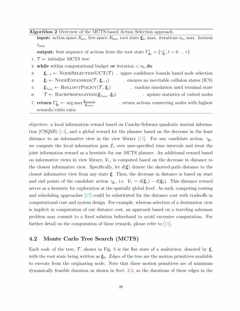
Algorithm 2 Overview of the MCTS-based Action Selection approach.
input: action space Xact, free space Xfree, root state ξ0, max. iterations nb, max. horizon
τmax
output: best sequence of actions from the root state Γ∗ξ0 = γ∗ξt , t = 0 . . . τ1: T ← initialize MCTS tree
2: while within computational budget or iteration < nb do
3: ξi−1 ← NodeSelectionUCT(T ) . upper confidence bounds based node selection
4: ξi ← NodeExpansion(T , ξi−1) . ensures no inevitable collision states (ICS)
5: ξτmax ← RolloutPolicy(T , ξi) . random simulation until terminal state
6: T ← Backpropagation(ξτmax , ξ0) . update statistics of visited nodes
7: return Γ∗ξ0 ← arg max ξrewards
ξvisits. return actions connecting nodes with highest
rewards/visits ratio
objective: a local information reward based on Cauchy-Schwarz quadratic mutual informa-
tion (CSQMI) [14], and a global reward for the planner based on the decrease in the least
distance to an informative view in the view library [15]. For any candidate action, γξt ,
we compute the local information gain Iγ over user-specified time intervals and treat the
joint information reward as a heuristic for our MCTS planner. An additional reward based
on informative views in view library, Vγ, is computed based on the decrease in distance to
the closest informative view. Specifically, let d(ξ) denote the shorted-path distance to the
closest informative view from any state ξ. Then, the decrease in distance is based on start
and end points of the candidate action γξt , i.e. Vγ = d(ξτ ) − d(ξ0). This distance reward
serves as a heuristic for exploration at the spatially global level. As such, competing routing
and scheduling approaches [17] could be substituted for the distance cost with tradeoffs in
computational cost and system design. For example, whereas selection of a destination view
is implicit in computation of our distance cost, an approach based on a traveling salesman
problem may commit to a fixed solution beforehand to avoid excessive computation. For
further detail on the computation of these rewards, please refer to [15].
4.2 Monte Carlo Tree Search (MCTS)
Each node of the tree, T , shown in Fig. 6 is the flat state of a multirotor, denoted by ξ,
with the root state being written as ξ0. Edges of the tree are the motion primitives available
to execute from the originating node. Note that these motion primitives are of minimum
dynamically feasible duration as shown in Sect. 3.3, so the durations of these edges in the
20
tree varies with the node they originate from.
Action selection proceeds as shown in Alg. 2. After initializing the tree with the root
state ξ0 (line 1), MCTS iterates until either a user specified number of maximum iterations
or a time budget (usually set by the planning rate) condition is violated. Within each
iteration, the tree is incrementally created in four steps. First, at line 3, a node with
unexpanded children is selected using a criteria based on Upper Confidence Bounds for
Trees (UCT) [3]. Second, from the resulting node, we choose a feasible action and expand
the tree from ξi−1 to ξi (line 4). Third, we insert nodes at random further down in the
tree until a state is reached where the limit on maximum horizon is exceeded (ξτmax , line 5).
And fourth, we backpropagate the node visits and reward statistics from ξτmax to the root
node ξ0 and continue further iterations (line 6). At the end, the sequence of nodes with
the highest rewards to visits ratio is returned as the most informative trajectory from the
current planning round (Γ∗ξ0).
As mentioned before, this report mainly contributes to the node expansion step (lines 4).
Specifically, we propose a node expansion approach that ensures no nodes in the tree are
visited from which the multirotor can not stop within the sensor range, rdepth. In this way, we
ensure that the robot never visits an inevitable collision state (ICS) [12]. Next, we describe
this safe node expansion approach.
4.3 Safety at High Speeds
Using the finite-horizon action representation developed in Sect. 3, we present a safe node
expansion algorithm that ensures the multirotor never reaches an inevitable collision state
(ICS), essential to maintain safety at high speeds in unknown environments [12]. The node
expansion policy for the proposed MCTS-based planning policy is shown schematically in
Alg. 3. Candidate actions from the current node ξi−1 are evaluated for expansion in three
steps. First, the candidate action is checked to lie in the explored free space Xfree (line 2).
Specifically, we create a truncated signed distance field (TSDF) from locations of occupied
and unknown spaces in the robot’s local map and inflate our lookups in this grid by a user-
specified collision radius, rcoll. Second, if the candidate action is inside Xfree, we sample a
dynamically feasible stopping trajectory using the minimum feasible duration method shown
in Sect. 3.3 at ∆tp (planning time) ahead of the current time (line 3). We choose this starting
time to ensure that we have a safe trajectory to track and bring the robot to halt within the
observed free space Xfree, in case the current planning round fails (further detail in Sect. 4.4).
Third, this stopping primitive γstopξtis checked for collisions (line 4) using the same TSDF
21
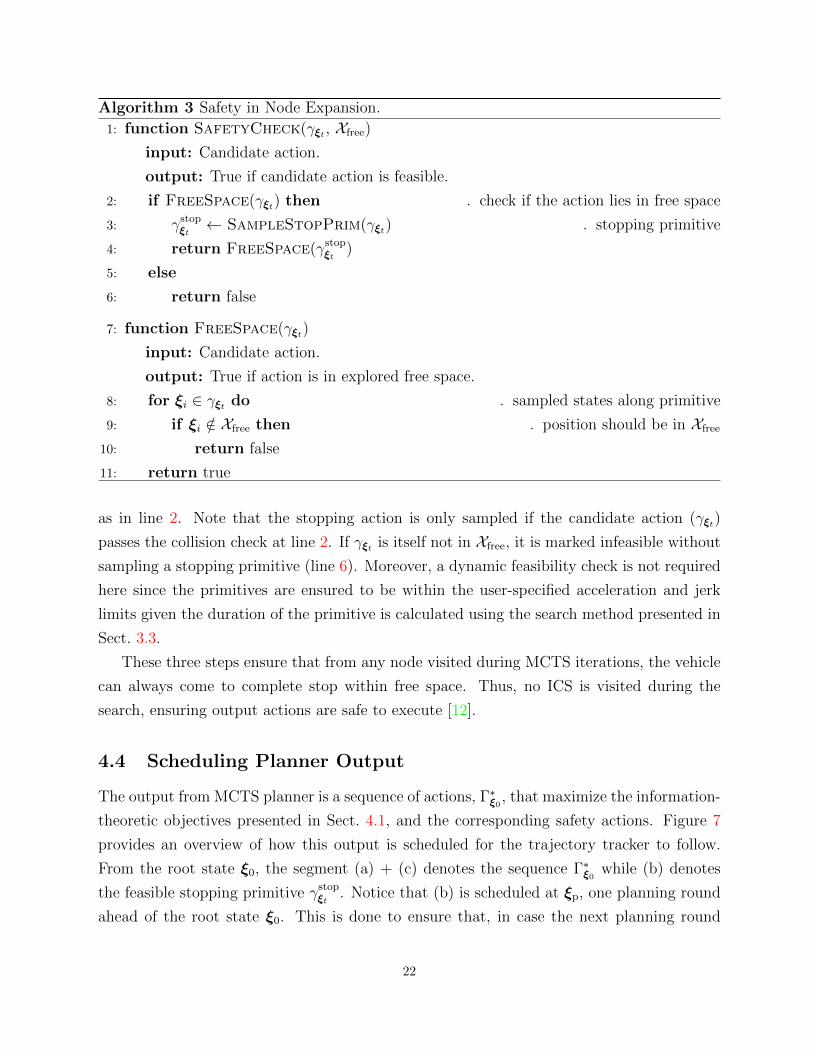
Algorithm 3 Safety in Node Expansion.
1: function SafetyCheck(γξt , Xfree)
input: Candidate action.
output: True if candidate action is feasible.
2: if FreeSpace(γξt) then . check if the action lies in free space
3: γstopξt← SampleStopPrim(γξt) . stopping primitive
4: return FreeSpace(γstopξt)
5: else
6: return false
7: function FreeSpace(γξt)
input: Candidate action.
output: True if action is in explored free space.
8: for ξi ∈ γξt do . sampled states along primitive
9: if ξi /∈ Xfree then . position should be in Xfree
10: return false
11: return true
as in line 2. Note that the stopping action is only sampled if the candidate action (γξt)
passes the collision check at line 2. If γξt is itself not in Xfree, it is marked infeasible without
sampling a stopping primitive (line 6). Moreover, a dynamic feasibility check is not required
here since the primitives are ensured to be within the user-specified acceleration and jerk
limits given the duration of the primitive is calculated using the search method presented in
Sect. 3.3.
These three steps ensure that from any node visited during MCTS iterations, the vehicle
can always come to complete stop within free space. Thus, no ICS is visited during the
search, ensuring output actions are safe to execute [12].
4.4 Scheduling Planner Output
The output from MCTS planner is a sequence of actions, Γ∗ξ0 , that maximize the information-
theoretic objectives presented in Sect. 4.1, and the corresponding safety actions. Figure 7
provides an overview of how this output is scheduled for the trajectory tracker to follow.
From the root state ξ0, the segment (a) + (c) denotes the sequence Γ∗ξ0 while (b) denotes
the feasible stopping primitive γstopξt. Notice that (b) is scheduled at ξp, one planning round
ahead of the root state ξ0. This is done to ensure that, in case the next planning round
22

(a)
(b)
(c)
Figure 7: Overview of safe node expansion in the proposed MCTS-planner and the scheduling
of stopping trajectories. Safety checks detailed in Alg. 3 and Sect. 4.3 ensure that all trajectory
segments (a), (b), and (c) lie in free space, Xfree. Segment (a) is scheduled at root node ξ0, while
segments (b) and (c) are scheduled at the end of the current planning round ξp. One of the segments
(b) or (c) are selected for tracking at ξp based on the output of the next planning round. This
approach to scheduling and safety checking ensures that the vehicle is always able to stop within
Xfree, even there is a failure in finding a feasible action during a one of the planning rounds.
fails, the trajectory tracker switches to tracking the segment (b) instead of (c) (which has
a non-zero end-point velocity). The segment (b) ensures that the vehicle stops within Xfree
with velocity and all higher-order derivatives zero at the end-point.
As described earlier in Sect. 3, these actions are 8th order polynomials in velocity, smooth
and continuous up to snap. Such high-order continuity ensures that there is no abrupt jump
in references for the trajectory tracker when switching between trajectory segments (for
example, from (a) to (b) in Fig. 7).
23

5 Results
(a) t = 0 s (b) t = 250 s
(c) t = 900 s (d) t = 1800 s
Figure 8: Different stages of exploration with respect to time for three-dimensional unstructured
environment considered for evaluation of the proposed motion planning framework. Black voxels
denote space marked as occupied. We consider a large room in 3D warehouse environment with
dimensions 60 m× 30 m× 11 m.
This section details the quantitative evaluation of the proposed exploration strategy. Specif-
ically, we demonstrate variation of exploration performance due to changes in action design
(Sect. 3) using the rate of reduction in Shannon entropy of the map [9]. For all experi-
ments, map is constructed using depth sensor data from the multirotor exploring a large
unstructured three-dimensional warehouse environment (see Fig. 8). In all our experiments,
we use the action representation presented in Sect. 3 and action selection strategy presented
in Sect. 4.
24

5.1 Simulation Experimentation Setup
In this section, various parametric details are presented that are common to all the experi-
ments conducted in the later sections. Specifically, we state the configurations for multirotor
inertial properties and constraints, sensing modality specifications, and assumptions in sim-
ulation experiments.
Table 3: Inertial properties and dynamics constraints for the multirotor used in the simulation
experiments.
Configuration Weight Thrust/Weight Amax Jmax
Value 30.45 N 3.5 10 m/s2 35 m/s3
5.1.1 Inertial and Sensing Parameters
Table. 3 lists a few of the critical dynamics parameters for the multirotor used in our exper-
iments. Intuitively, to be able to execute fast actions on a multirotor, we need a high thrust
to weight ratio to be able to change attitude of the multirotor rapidly. Therefore, we use
the parameters from the high speed teleoperation platform presented in Spitzer et al. [1].
Furthermore, empirically determined acceleration (Amax) and jerk (Jmax) constraints for this
platform are taken into account in both the proposed action representation (Sect. 3) and
action selection (Sect. 4).
Table 4: Sensing constraints for the forward facing depth camera used in for the exploration
experiments.
Configuration rdepth Rate Width Height Noise
Value 5.0 m 10 Hz 160 pixels 120 pixels N/A
Following inertial constraints, we now list key sensing modality parameters and con-
straints in Tab. 4. We use a single forward facing depth sensor for all experiments with
maximum range capped at rdepth. To enable a faster mapping rate we keep the rate of sen-
sor observations at 10 Hz. For all sensor observations, we do not consider noise in depth
measurements to keep the focus on planning in a deterministic map.
25

Table 5: Average rates at which various types of high and low speed primitives are selected by
the action selector. These rates are calculated after averaging number of primitives selected of the
said type with respect to the total number of planning rounds across trials.
Experiments ⊥ ‖ Stop Yaw High Low
E1: ‖,⊥, low speed 0.30 0.57 8.85× 10⁻⁴ 0.13 - 1.0
E2: ⊥, low speed 0.57 - 3.40× 10⁻³ 0.43 - 1.0
E3: ⊥, high speed 0.54 - 6.80× 10⁻³ 0.45 0.31 0.69
E4: ‖,⊥, high speed 0.45 0.25 0.01 0.29 0.54 0.46
5.1.2 Triggered Simulation
To analyze variation in exploration performance due to increasing planning rates and finite-
horizon lengths, we trigger the simulation based on the time taken by the planner. Specifi-
cally, number of iterations taken by the MCTS planner is kept consistent across trials and the
simulation clock is slowed down to accommodate it accordingly. All trials are 2500 seconds
in duration with robots starting at different initial positions in the environment.
5.2 Effects of Action Design
In this section, we identify the effects of the variation in available motion primitive libraries
that are available to the MCTS planner have on the following experiments (all experiments
were performed using a MCTS-based planner with a 2 second planning horizon):
• E1: Action design with low speed actions in both perpendicular and parallel directions
to the sensor observation, no high speed actions.
• E2: Action design with low speed actions in only perpendicular direction to the sensor
observation, no actions in parallel direction.
• E3: Action design with low and high speed actions in perpendicular direction to the
sensor observation, no actions in parallel direction.
• E4: Action design with low and high speed actions in perpendicular direction, while
only high speed actions in parallel direction to the sensor observation.
26

0 500 1,000 1,500 2,000 2,500
500
1,000
1,500
2,000
Time (s)
Entrop
yreductionrate
(bits/s) E1: ‖, ⊥, low speed
E2: ⊥, low speed
(a) Effect of ‖ direction at low speed
500 1,000 1,500 2,000 2,5000
500
1,000
1,500
2,000
Time (s)
Entropyreductionrate
(bits/s) E2: ⊥, low speed
E3: ⊥, high speed
(b) Speed comparison in ⊥ direction
0 500 1,000 1,500 2,000 2,5000
500
1,000
1,500
2,000
2,500
Time (s)
Entrop
yreductionrate
(bits/s) E3: ⊥, high speed
E4: ‖, ⊥, high speed
(c) Effect of ‖ direction at high speed
500 1,000 1,500 2,000 2,500
500
1,000
1,500
2,000
2,500
Time (s)
Entrop
yreductionrate
(bits/s) E1: ‖, ⊥, low speed
E4: ‖, ⊥, high speed
(d) Speed comparison in both directions
Figure 9: Rate of exploration variations with time to investigate effects of changes in action
design on exploration performance. We observe substantial improvement in performance due to
availability of parallel motions (a, c), while performance increment due to high speed perpendicular
actions is observed to be minimal (b, d).
Comparison between exploration performance across these experiments is shown in Fig. 9.
As we have shown in the idealized analysis (Sect. 2), parallel actions also influence entropy
reduction rate (measured in bits/s) significantly in addition to actions perpendicular to a
frontier or a sensor observation in general. This analysis is reflected in the results shown in
27

Fig. 9a, where the use of parallel direction primitives in experiment sets E1, E4 provides a
nearly 1.5 times improvement in entropy reduction performance over E2 and E3 respectively
(see Fig. 9a and Fig. 9c). This behavior is expected since parallel motions have a larger
effective area during exploration and are allowed to achieve higher speeds than perpendicular
actions (Sect. 2). However, introducing high speed actions in either directions seems to
impart only a little advantage over the low speed actions (see Fig. 9b and Fig. 9d), which is
in contrast to our analysis in Sect. 2.
We can investigate why including a high speed action representation not been effective
in exploration performance, by looking at the rate at which a particular type of primitive is
selected. Table 5 shows these rates for each of the experiments averaged across trials. For
E3, we observe that only about one-third of the high speed primitives are actually selected by
the planner, while for E4 we observe about half of them being chosen. This follows from our
earlier observation in Sect. 2 that in perpendicular direction to a frontier, the motion planner
favors slower actions due to the safety constraints. In addition, comparing E1 and E4, there
is a 2 times decrease in the probability of a parallel direction primitive being selected. This
means that at higher speeds, the action selector is not able to select parallel actions as often
as at low speeds. These two factors counteract each other, leaving a negligible performance
increment due to higher speeds. We currently suspect that this behavior is either due to
enhanced feasibility constraints at higher speeds or excessive length of the motion primitive
library available to the finite horizon planner, see the limitations section (Sect. 6) for further
discussion.
28

500 1,000 1,500 2,000
500
1,000
1,500
2,000
2,500
Time (s)
Entrop
yreductionrate
(bits/s) 1 Hz
2Hz5Hz0.5Hz
(a) Entropy reduction rate
500 1,000 1,500 2,0000
0.5
1
1.5
·106
Time (s)
EntropyReduction(bits)
1 Hz2Hz5Hz0.5Hz
(b) Entropy reduction
Figure 10: Results for effects of planning rate on exploration performance in a three-dimensional
scenario. Two metrics, entropy reduction rate (a) and entropy reduction (b), are shown with re-
spect to time. We observe a peculiar behavior – entropy reduction rate maximizes for 1 Hz planning
rate, performing better than 2 Hz and 5 Hz. Furthermore, a substantial part of the environment is
left unexplored at 0.5 Hz (b).
5.3 Effects of Planning Rate
This section deals with analyzing exploration performance with changing replanning rate. As
analyzed in Sect. 2, faster rate of planning means the multirotor can execute higher velocity
actions while remaining anytime safe. Thus, the rate of exploration should increase as we
move towards faster planning rates. To this end, using our simulation setup, we conduct the
2500 seconds long trials with planning rates 0.5 Hz, 1 Hz, 2 Hz, and 5 Hz. Note that all trials
in these experiments use the action design used in experiment E4 previously.
We observe that the exploration performance peaks at 1 Hz, while the performance at
0.5 Hz degrades to an extent that a significant part of the environment is left unexplored
(Fig. 10). In contrast to our analysis in Sect. 2, the entropy reduction rate does not get better
with increasing planning rate after 1 Hz. This result does not follow the expected behavior
shown in Sect. 2. The cause of this trend might be linked with the high speed primitives not
being effective in increasing exploration performance, as suggested in the preceding section.
However, further investigation is required to get a better insight into this variation, and we
leave it as a future work.
29

500 1,000 1,500 2,000
500
1,000
1,500
2,000
Time (s)
Entrop
yreductionrate
(bits/s) 2 s
4 s
(a) Entropy reduction rate
500 1,000 1,500 2,0000
0.2
0.4
0.6
0.8
1·106
Time (s)
Entrop
yReduction(bits)
2 s4 s
(b) Entropy reduction
Figure 11: Variation in length of the finite-horizon and its effects on exploration performance in
a two-dimensional scenario. Two metrics, entropy reduction rate (a) and entropy reduction (b),
are shown with respect to time. As expected, longer finite horizon results in significantly better
exploration rate (here we compare 2 second with a 4 second horizon).
5.4 Effects of Finite-Horizon Length
As detailed in Sect. 4, we use a Monte-Carlo Tree Search (MCTS) based finite horizon
planning strategy to select actions that are feasible and maximize information gain. In
this section, effects of the horizon length of this receding-horizon planner on the exploration
performance are analyzed. We start with a simplified two-dimensional scenario, where action
space is constrained to lie only in the xB−yB plane (so, no motion primitives in zB direction).
In Fig. 11, results for simulation experiments at two different horizon lengths – 2 and 4
seconds – are shown. For a 4 seconds horizon, exploration rate is nearly 75% faster than
that of 2 seconds case during the first 800 seconds of exploration.
It is worth noting here that as the horizon length increases, the computational cost per
planning iteration of our MCTS-based planner also increases significantly. Thus, there is a
trade-off between computational complexity and the exploration performance that needs to
be considered while trying to use this planner in a real time use case.
30
6 Conclusion
6.1 Contributions
We presented three main contributions in this report. First, we analyzed how exploration
performance varies using a few idealized scenarios considering constraints on dynamics and
sensing for a multirotor vehicle. Second, we proposed a strategy to design candidate actions
for the motion planner that accounts for platform dynamics and provides actions that are
useful for rapid exploration based on the prior analysis. Third, we presented a receding-
horizon sampling-based planner that uses this action representation, maximizes information
gain, and ensures safe operation at high speeds. Finally, through extensive simulation ex-
periments in a complex three-dimensional environment, we demonstrated the significance of
action design, finite-horizon length, and replanning rate on exploration performance.
6.2 Limitations & Future Work
Sect. 5 highlights a few limitations in our current approach to action representation (Sect. 3)
and action selection (Sect. 4). First, the variation in the exploration performance due to
increase in planning rate is in contrast to the ideal exploration analysis in Sect. 2. We note
that the cause of this behavior might be due to excessive length of the primitives in perpen-
dicular direction at higher speeds. Another reason might include large spaces between poses
on which CSQMI is evaluated. One solution might be discounting the information rewards
with respect to time. Second, the computational cost of our MCTS-based action selection
strategy scales with the number of desired iterations as well as finite-horizon length. Solving
this limitation might require using intelligent biasing techniques to search for informative
regions in the search tree and hence generate a better planning policy in lesser number of
iterations.
31
References
[1] A. Spitzer, X. Yang, J. Yao, A. Dhawale, K. Goel, M. Dabhi, M. Collins, C. Boirum, and
N. Michael, “Fast and agile vision-based flight with teleoperation and collision avoidance
on a multirotor,” in Proc. of the Intl. Sym. on Exp. Robot. Buenos Aires, Argentina:
Springer, 2018, to be published.
[2] G. Chaslot, “Monte-Carlo tree search,” Ph.D. dissertation, Universiteit Maastricht,
2010.
[3] C. Browne, E. Powley, D. Whitehouse, S. Lucas, P. I. Cowling, P. Rohlfshagen,
S. Tavener, D. Perez, S. Samothrakis, and S. Colton, “A survey of Monte Carlo tree
search methods,” IEEE Trans. on Comput. Intell. and AI in Games, vol. 4, no. 1, pp.
1–43, 2012.
[4] M. Corah and N. Michael, “Distributed matroid-constrained submodular maximization
for multi-robot exploration: theory and practice,” Auton. Robots, 2018.
[5] N. Michael, S. Shen, K. Mohta, Y. Mulgaonkar, V. Kumar, K. Nagatani, Y. Okada,
S. Kiribayashi, K. Otake, K. Yoshida, K. Ohno, E. Takeuchi, and S. Tadokoro, “Col-
laborative mapping of an earthquake-damaged building via ground and aerial robots,”
J. Field Robot., Jun. 2012.
[6] T. Cieslewski, E. Kaufmann, and D. Scaramuzza, “Rapid exploration with multi-rotors:
A frontier selection method for high speed flight,” in Proc. of the IEEE/RSJ Intl. Conf.
on Intell. Robots and Syst., Vancouver, Canada, Sep. 2017.
[7] S. Liu, M. Watterson, S. Tang, and V. Kumar, “High speed navigation for quadrotors
with limited onboard sensing,” in Proc. of the IEEE Intl. Conf. on Robot. and Autom.,
Stockholm, Sweden, May 2016.
[8] B. Yamauchi, “A frontier-based approach for autonomous exploration,” in Proc. of the
Intl. Sym. on Comput. Intell. in Robot. and Autom., Monterey, CA, Jul. 1997.
[9] T. M. Cover and J. A. Thomas, Elements of Information Theory. New York, NY: John
Wiley & Sons, 2012.
[10] N. Michael, D. Mellinger, Q. Lindsey, and V. Kumar, “The grasp multiple micro-uav
testbed,” IEEE Robot. Autom. Mag., vol. 17, no. 3, pp. 56–65, 2010.
32

[11] R. Mahony, V. Kumar, and P. Corke, “Multirotor aerial vehicles,” IEEE Robot. Autom.
Mag., vol. 20, no. 32, 2012.
[12] L. Janson, T. Hu, and M. Pavone, “Safe motion planning in unknown environments:
Optimality benchmarks and tractable policies,” in Proc. of Robot.: Sci. and Syst., Pitts-
burgh, PA, Jul. 2018.
[13] D. Mellinger and V. Kumar, “Minimum snap trajectory generation and control for
quadrotors,” in Proc. of the IEEE Intl. Conf. on Robot. and Autom., Shanghai, China,
May 2011.
[14] B. Charrow, S. Liu, V. Kumar, and N. Michael, “Information-theoretic mapping using
Cauchy-Schwarz quadratic mutual information,” in Proc. of the IEEE Intl. Conf. on
Robot. and Autom., Seattle, WA, May 2015.
[15] M. Corah, C. O’Meadhra, K. Goel, and N. Michael, “Communication-efficient planning
and mapping for multi-robot exploration in large environments,” IEEE Robot. Autom.
Letters, 2019, submitted for publication.
[16] M. Lauri and R. Ritala, “Planning for robotic exploration based on forward simulation,”
Robot. Auton. Syst., vol. 83, 2016.
[17] M. Kulich, J. Faigl, and L. Preucil, “On distance utility in the exploration task,” in
Proc. of the IEEE Intl. Conf. on Robot. and Autom. Shanghai, China: IEEE, May
2011.
33


![[2] compl-alg](https://static.fdocuments.in/doc/165x107/55cf8df5550346703b8d16ff/2-compl-alg.jpg)