Technical Report - Polytechnique Montréal

LATTICE REFORMULATIONS CUTS

Karen Aardal

Frederik von Heymann

Andrea Lodi

Andrea Tramontani

Laurence A. Wolsey

July 2018

DS4DM-2018-003

POLYTECHNIQUE MONTRÉAL

DÉPARTEMENT DE MATHÉMATIQUES ET GÉNIE INDUSTRIEL

Pavillon André-Aisenstadt Succursale Centre-Ville C.P. 6079 Montréal - Québec H3C 3A7 - Canada Téléphone: 514-340-5121 # 3314

Mathematical Programming manuscript No.(will be inserted by the editor)

Lattice Reformulation Cuts

Karen Aardal · Frederik von Heymann ·Andrea Lodi · Andrea Tramontani ·Laurence A. Wolsey

Received: date / Accepted: date

Abstract Here we consider the question whether the lattice reformulation ofa linear integer program can be used to produce effective cutting planes. Weconsider integer programs (IP) in the form max{cx | Ax = b,x ∈ Zn

+} , wherethe reformulation takes the form max{cx0 + cQµ | Qµ ≥ −x0, µ ∈ Zn−m} ,where Q is an n× (n−m) integer matrix. Working on an optimal LP tableauin the µ-space allows us to generate n−m Gomory mixed-integer inequalities(GMIs) in addition to the m GMIs associated with the optimal tableau in thex space. These provide new cuts that can be seen as GMIs associated to n−mnon-elementary split directions associated with the reformulation matrix Q.On the other hand it turns out that the corner polyhedra associated to an LPbasis and the GMI or split closures are the same whether working in the x or µspaces. Computationally we show that the effectiveness of the cuts generatedby this approach depends on the quality of the reformulation obtained bythe reduced basis algorithm used to generate Q and that it is worthwhile togenerate several rounds of such cuts. However, the effectiveness of the cutsdeteriorates as the number of constraints is increased.

The research has been financed in part by The Netherlands Organisation for ScientificResearch, NWO, grant number 613.000.801, which we gratefully acknowledge.

K. AardalDelft University of Technology, The Netherlands. E-mail: [email protected]

F. von HeymannUniversity of Cologne, Germany. E-mail: [email protected]

A. LodiCERC, Ecole Polytechnique de Montreal, Canada. E-mail: [email protected]

A. TramontaniCPLEX Optimization, IBM, Italy. E-mail: [email protected]

L.A. WolseyUniversite catholique de Louvain, Belgium. E-mail: [email protected]

CERC DATA SCIENCE FOR REAL-TIME DECISION-MAKING DS4DM-2018-003

2 K. Aardal, F. von Heymann, A. Lodi, A. Tramontani, L.A. Wolsey

Keywords Integer programming · Cutting planes · lattice reformulation ·lattice basis reduction

Mathematics Subject Classification (2010) 90C10 · 11H06

1 Introduction

In a series of papers Aardal et al. [1–4] have shown that certain integer pro-grams that cannot be solved by a standard MIP solver can be solved by usinga lattice-reformulation of the problem. This raises the question studied hereof whether such a lattice-reformulation can also be used to produce effectivecutting planes.

Specifically we consider pure integer programs (IP) in the form

max{cx | Ax = b,x ∈ Zn+} , (1)

where A ∈ Zm×n, b ∈ Zm, c ∈ Zn, and where we let P = {x ∈ Rn+ | Ax = b}

and S = P ∩ Zn.The reformulation takes the form

max{cx0 + cQµ | Qµ ≥ −x0, µ ∈ Zn−m} , (2)

where Q is an n× (n−m) integer matrix and x0 is a point satisfying Ax0 =b, x0 ∈ Zn. Here we let P = {µ ∈ Rn−m : Qµ ≥ −x0} and S = P ∩ Zn−m.The integer sets S and S are related: x ∈ S if and only if there exists µ ∈ Swith x = x0 +Qµ, or in other words S =projx{(x,µ) : x = x0 +Qµ,µ ∈ S}.

The intuition behind our approach is that the polytope P has a regularshape in the sense that it does not have an obvious thin direction, if P is createdafter a basis reduction process ofQ, and that therefore split disjunctions in thecoordinate directions of P are potentially interesting. This idea is supportedby the computational experience with branch and bound on P rather thanon P . Branching in unit directions on P has proven to be computationallymore effective for certain problem types, see e.g. [2,3]. Thus our motivationis to look for Gomory Mixed-Integer (GMI) cuts [20] that are not necessarilytableau cuts for P , but are still computationally easy to generate.

A first practical observation is that if one considers the reformulated prob-lem (2), one can generate (n−m) new Chvatal-Gomory (CG) [10] or GMI cutsoff an optimal linear program (LP) tableau. Here we will concentrate on GMIcuts (also viewed as split cuts [12]). These will be called (lattice) `-cuts. Thisraises a series of questions both theoretical and computational. For example:

- What is the relationship between P and P?- Given a point µ ∈ S, what is the corresponding point x ∈ S?- What do the `-cuts in the µ-space give in the x-space?- Are the corner polyhedra associated to a basis in the x and µ spaces the

same?- What, if any, is the relationship between the GMI or split closures of P

and P?


Lattice Reformulation Cuts 3

Computational questions that we investigate are:

- How effective are the `-cuts?- Can the `-cuts associated to a basis tableau be easily generated in thex-space?

We now point to some related computational work. Bixby et al. [7] ob-served that one round of GMI inequalities generated from an optimal basicsolution closed 24% of the integrality gap on average on 41 MIPLIB instances.Cornuejols et al. [14] suggested to multiply a row in the optimal LP tableauby an integer k, and then derive a GMI off of the resulting row. They calleda cut generated in this way a k-cut. The standard tableau GMI inequalityis a k-cut with k = 1. One motivation behind this approach is to create alarge fractional right-hand side of the resulting tableau row as this intuitivelycould lead to a stronger inequality. Later Cornuejols [13] suggested that oneshould look for deep split cuts that can be separated efficiently. This is alsothe viewpoint taken here.

An alternative, but very costly approach, is to generate all the inequalitiesfrom a given family, known as the closure. Balas and Saxena [6] performeda computational study of the split inequalities and concluded that the splitclosure closed 82% of the integrality gap, on average, on 33 mixed integerMIPLIB instances, and 71%, on average, on 24 pure integer MIPLIB instances.It is, however, NP-hard to optimize a linear function over the split closure[9], so achieving these results is computationally expensive. Of course, a vastliterature has been devoted to computationally viable ways of approximatingthe split closure, see, e.g., Dash and Goycoolea [16] and Fischetti and Salvagnin[19].

In Section 2 we present the background material we need concerning in-equalities and lattices. In Section 3 we see that most of the theoretical ques-tions have simple and perhaps surprising answers. In particular, even thoughthe GMI/split cuts generated may be different, the GMI/split closures are thesame. We give a description of our approach for generating violated inequal-ities in Section 4 and present our computational results comparing differentpossible variants in Section 5. Finally, some conclusions are drawn in Section6.

2 Background

2.1 Gomory mixed integer inequalities and split inequalities

We define Gomory mixed-integer inequalities (GMI) and split inequalities, k-cuts and closures. For a more general exposition we refer to [11,27].

Consider the single row mixed-integer set

X = {(x,y) ∈ Zn+ × Rp

+ |n∑

j=1

ajxj +

p∑j=1

gjyj = b} (3)



and suppose that b 6∈ Z. Let

b := bbc+ f0 with 0 < f0 < 1,aj := bajc+ fj with 0 ≤ fj < 1.

The Gomory mixed-integer (GMI) inequality [20] for X is

∑{j:fj≤f0}

fjf0xj +

∑{j:fj>f0}

1− fj1− f0

xj +∑

{j:gj>0}

gjf0yj−

∑{j:gj<0}

gj1− f0

yj ≥ 1 . (4)

If the row (3) is a row from a simplex tableau of a linear relaxation, theassociated GMI inequality is referred to as a tableau GMI inequality.

Cornuejols et al. [14] introduced k-cuts, which are cuts that are obtained byfirst multiplying (3) from an optimal tableau in which one of the x-variables isbasic by an integer k, and then deriving the GMI inequality. In this paper weintroduce `-cuts, which are tableau GMI cuts derived from an optimal tableauof the LP-relaxation of (2). In Sections 3 and 4 we explain how to generatethese cuts in the space of the x-variables.

Let T be a polyhedron in Rn+p. Next, we consider a mixed integer setT ∩ (Zn × Rp). For given (π, π0) ∈ Zn+1 we define

Π1 := T ∩ {(x,y) ∈ Zn × Rp | πx ≤ π0}Π2 := T ∩ {(x,y) ∈ Zn × Rp | πx ≥ π0 + 1} .

An inequality αx+ γy ≤ β is called a split inequality [12] if there exists a(π, π0) ∈ Zn+1 such that αx + γy ≤ β is valid for Π1 ∪Π2. The disjunctionπx ≤ π0∨πx ≥ π0+1 is called a split disjunction. The GMI inequality can beviewed as a split inequality for (3) with the split in which πj = bajc if fj ≤ f0,πj = daje if fj > f0 and π0 = bbc.

The elementary closure, or simply the closure, associated with a familyF of inequalities valid for T ∩ (Zn × Rp) is the convex set obtained as theintersection of all inequalities in F . Not surprisingly, the GMI and split closuresare equivalent [28]. The separation problem for the split closure is NP-hard[9].

Later we will encounter single row sets X both in the all integer case andin the mixed integer case in which we add GMI cuts containing slack variablesthat are not integer variables.

Observation 1 If X is replaced by

X = {(x,y) ∈ Zn+ × Rp

+ |n∑

j=1

ajxj +

p∑j=1

gjyj = b} ,

where aj ≡ aj mod 1 for 1 ≤ j ≤ n and b ≡ b mod 1, the GMI (4) for Xand the GMI for X are the same inequality.



2.2 Lattices and lattice reformulation

Given l ≤ n linearly independent vectors b1, . . . bl ∈ Rn, the set L(b1, . . . , bl) :=

{∑l

i=1 cibi, ci ∈ Z} is called the lattice generated by b1, . . . bl. The vectorsb1, . . . bl are called a lattice basis, and we often represent them as a matrixB = (b1, . . . bl). Given a lattice L generated by B, the basis B′ is an alter-native basis for L if and only if we can write B′ = BU , where U is an l × lunimodular matrix.

We now can explain the reformulation of the integer program

max{cx | Ax = b, x ∈ Zn+}, (1)

presented in the Section 1, due to Aardal et al. [1]. The set kerZ(A) = {x ∈Zn | Ax = 0} is a lattice, called the kernel lattice of A.

Suppose x is a feasible solution in problem (1). If x0 ∈ Zn satisfies Ax0 =b, it follows that A(x− x0) = 0 and thus, if Q is a lattice basis for kerZ(A),this is equivalent to (x − x0) = Qµ where µ ∈ Zn−m. Now substitutingx = x0 +Qµ and using x ≥ 0 gives the reformulation

max{c(x0 +Qµ) | Qµ ≥ −x0,µ ∈ Zn−m} . (2)

Let L be a lattice in a Euclidean vector space E. A subset K ⊆ L iscalled a pure sublattice of L if there exists a linear subspace D of E such thatK = D ∩ L.

A matrix A ∈ Zm×n of full row rank is in Hermite Normal Form if it hasthe form HNF(A) = (H,0m×(n−m)) = AU , where H is a lower triangularnonnegative m × m matrix in which the unique row maxima can be foundalong the diagonal, and U is an n× n unimodular matrix.

Observation 2 A lattice L generated by the basis B = (b1, . . . , bl) is a puresublattice of the standard lattice Zn if and only if HNF(BT) = (I,0).

Observation 3 The lattice kerZ(A) is a pure sublattice of Zn.

Theorem 1 (See Schrijver [29], Theorem 5.2.) The Hermite NormalForm (H,0) of a rational matrix A of full row rank has size polynomiallybounded by the size of A. Moreover, there exists a unimodular matrix U withAU = (H,0), such that the size of U is polynomially bounded by the size ofA.

Proposition 1 (See Schrijver [29], Corollary 5.3a.) Given a rationalmatrix A of full row rank, a unimodular matrix U such that AU is in HermiteNormal Form can be found in polynomial time.

3 Relations between solutions and polyhedra in x- and µ-space

Here we establish answers to the theoretical questions raised in the introduc-tion.



3.1 Expressing µ ∈ S as a function of x ∈ S

The lattice reformulation gives a way of expressing each feasible vector x ∈ Sas a function of µ. A natural question is how to express a feasible vectorµ ∈ S as a function of x. In particular, this is our prime tool for generatinggeneral disjunctions for deriving split inequalities, as described in more detailin Section 4.

A consequence of kerZ(A) being a pure sublattice of Zn, and of Theorem1 and Proposition 1, is that we can find, in polynomial time, a unimodularmatrix U such that

UTQ =

(I

0

). (5)

Let W be the matrix consisting of the first n−m rows of UT as in (5). SinceW is a submatrix of UT it follows that all elements of W are integral. It isalso clear that

WQ = I . (6)

This was also observed by Mehrotra and Li [26]. Note that W in general is notunique: given a matrix W , we can form a matrix W ′ = W +C, where C isan integer (n−m)×n matrix consisting of rows obtained by taking an integerlinear combination of rows of A. The matrix W permits us to translate anexpression in µ-variables back to an expression in x-variables. Specifically wehave Wx = Wx0 +WQµ and thus

µ = Wx−Wx0 .

3.2 Relations between polyhedra in the x- and µ-spaces

Here we show that not only vectors in S and S correspond one-to-one, butthat there is also a one-to-one correspondence between vectors in P and P .

Proposition 2 Given A ∈ Zm×n and b ∈ Zm, define P = {x ∈ Rn+ | Ax =

b}. We can write x ∈ P ∩Zn as x = x0 +Qµ, where x0, Q, and µ are definedas in Section 2. Define P = {µ ∈ Rn−m | Qµ ≥ −x0} for Q and x0 as givenabove. The map f(µ) = Qµ+ x0 is a bijective map from P to P .

Proof Take µ ∈ P and let x = Qµ + x0. The vector x is nonnegative sinceQµ ≥ −x0. Moreover, Ax = AQµ + Ax0 = Ax0 = b, where the secondequality holds since Q is a basis for kerZ(A).

Take x ∈ P . Since Q spans the Euclidean vector space {x ∈ Rn | Ax = 0},we can write x as x = Qµ + x0 for some µ ∈ Rn−m. x ∈ P implies x ≥ 0,and hence Qµ+ x0 ≥ 0, so µ ∈ P . ut

Given an LP-basis, we examine the corresponding partitions of A,Q andW .



Proposition 3 Given A,Q,W as described above and an LP-basis B in x-space, write A = (B,N), QT = (QB ,QN ), W = (WB ,WN ) and Bx0

B +Nx0

N = b.For QB and QN the following holds:

i) QB = −B−1NQN ,ii) Q−1N = WN −WBB

−1N .

Proof i) AsAQ = 0,BQB+NQN = 0 and, asB−1 exists,QB = −B−1NQN .

ii) As WQ = I, WBQB +WNQN = I, and using i), one has (−WBB−1N +

WN )QN = I. It follows as QN and WN−WBB−1N are both (n−m)×(n−

m) matrices that QN is non-singular and thus Q−1N = WN −WBB−1N . ut

Now we consider the representation of the basis in the x- and µ-spaces.A basic solution in the x-space is written as

xB +B−1NxN = B−1b, xB ,xN ≥ 0 .

Writing the reformulation in equality form we observe that the x-variablesare precisely the slack variables, i.e.,

x−Qµ = x0 ,

which we can write as (xB

xN

)−(QB

QN

)µ =

(x0B

x0N

). (7)

Since the µ-variables are free, they must be basic and thus the basic variablesare (xB ,µ). Multiplying the last n−m rows of (7) by −Q−1N yields

−Q−1N xN + Iµ = −Q−1N x0N , or equivalently µ = Q−1N xN −Q−1N x0

N .

Substituting for µ in the first m rows of (7) gives

xB −QBQ−1N xN = x0

B −QBQ−1N x0

N ,

and we obtain an expression for a basic solution:(xB

µ

)−(QBQ

−1N

Q−1N

)xN =

(x0B −QBQ

−1N x0

N

−Q−1N x0N

). (8)

Now using Proposition 3, the basic solution (8) can be rewritten as(xB

µ

)+

(B−1N

−(WN −WBB−1N)

)xN =

(x0B +B−1Nx0

N

−(WN −WBB−1N)x0

N

)

=

(B−1b

−(WN −WBB−1N)x0

N

). (9)

From (8) we see that, given an LP-basis, the µ-variables can be expressedsolely as a function of Q.

We now illustrate the different basis representations in an Example.



Example 1 Consider an instance with m = 2, n = 5,

(A | b) =

(0 5 3 1 7 96 3 0 11 2 14

).

To obtain a reformulation, one can take

Q =

1 −3 −33 3 00 −3 4−1 1 2−2 −1 −2

, x0 =

01110

.

A matrix W corresponding to Q is:

W =

−2 −1 0 −4 −1−2 1 1 −3 2−3 0 1 −5 1

.

For the feasible basis xB = (x1, x2), the corresponding x-tableau is:(x1x2

)+

1

30

(−9 52 −1118 6 42

)x3x4x5

=1

30

(4354

).

Now setting µ = Wx −Wx0 and eliminating the basic variables xB bysubstitution, the corresponding µ-tableau is:µ1

µ2

µ3

− 1

30

0 −10 −10−6 8 −4

3 6 −3

x3x4x5

=1

30

10−2−9

.

From the µ3 row, one has f3 = 2730 , f4 = 24

30 , f5 = 330 and f0 = 21

30 giving the`-cut:

1

3x3 +

2

3x4 +

1

7x5 ≥ 1.

ut

We now turn our attention to the group problem associated with the twoformulations, and the related corner polyhedra [21]. LetA = (B, N), whereBcorresponds to the basic variables in an optimal solution to the LP-relaxationof (1). The following integer optimization problem is a relaxation of (1) ob-tained by dropping the nonnegativity constraints on the basic variables xB .

max{cx | (B N)

(xB

xN

)= b, xN ≥ 0, xB ,xN integral} . (10)

Using the relation BxB + NxN = b and the integrality of xB gives theequivalent formulation of (10) as:

max{cBB−1b+(cN−cBB−1N)xN | B−1NxN ≡ B−1b mod 1, xN ∈ Zn−m+ } .(11)



Problem (11) is referred to as the group problem [21].We will now prove that the feasible sets of the group problem is the same

whether we view it in the original x-space or in the reformulated space.

Theorem 2 The group problems arising in the x- and µ-spaces are the same.

Proof We consider the feasible regions corresponding to the underlying groups.Let

G = {xN ∈ Zn−m+ | B−1NxN ≡ B−1b mod 1}

and

G = {xN ∈ Zn−m+ | −(WN−WBB

−1N)xN ≡ −(WN−WBB−1N)x0

N mod 1}.

As WNxN ,WNx0N are integer,

G = {xN ∈ Zn−m+ |WBB

−1NxN ≡WBB−1Nx0

N mod 1}. (12)

Now as WB is an integral matrix, it follows that G ⊆ G.Conversely, take G in the form (see (8)):

G = {xN ∈ Zn−m+ | Q−1N xN ≡ Q−1N x0

N mod 1},

Suppose xN ∈ G. As QB is an integer matrix, xN lies in

{xN ∈ Zn−m+ | QBQ

−1N xN ≡ QBQ

−1N x0

N mod 1} ,

which, as QBQ−1N = −B−1N , is precisely G. ut

As the order of the groups is given by the determinant, it follows that|det(B)| = |det(QN )| and as the corner polyhedron is the convex hull ofthe solutions to the group problem, it follows immediately that the cornerpolyhedra are the same.

Based on Observation 1, we see that the `-cuts generated from the secondset of equations of (8), the second set of equations of (9) or from (12) are thesame.

Observation 4 Taking µ = W (x− x0) or µ′ = WB(xB − x0B) leads to the

same `-cuts because WNxN = 0 mod 1 and WNx0N = 0 mod 1. Therefore

a simple way to obtain the `-cuts is to left multiply the x-tableau by WB. Itfollows that WB is an m-dimensional generalization of the k in k-cuts. Inparticular, if m = 1, taking k = WB gives us a specific choice for k. On theother hand, if m > 1, the `-cuts can be viewed as multi-row tableau cuts, seee.g. [15].

Now we consider closures. Let PS (PCG ) be the split (Chvatal-Gomory)closure with respect to P . Analogous notation is used for P . We show that thesplit closures associated with P and P are equivalent.

Theorem 3 PS = {x ∈ Rn | x = x0 +Qµ, µ ∈ PS}.



Proof We use the definition of split cuts [12]. Let (π, π0) ∈ Zn+1 and let

αx− q(πx− π0) ≤ α0

αx+ r(πx− π0 − 1) ≤ α0

be valid inequalities for P with q, r ≥ 0. Then, αx ≤ α0 is valid for(P ∩ {πx ≤ π0}) ∪ (P ∩ {πx ≥ π0 + 1}). The inequality αx ≤ α0 is called asplit cut.

Substitute x for Qµ+ x0. Let

π = πQ ,

π0 = π0 − πx0 ,

α = αQ ,

α0 = α0 −αx0 .

Notice that (π, π0) ∈ Zn−m+1 as Q and x0 are integer. We obtain

αµ− q(πµ− π0) ≤ α0 (13)

αµ+ r(πµ− π0 − 1) ≤ α0 . (14)

If inequalities (13) and (14) are valid for P , then αµ ≤ α0 is valid for(P ∩ {πµ ≤ π0}) ∪ (P ∩ {πµ ≥ π0 + 1}).

Going from a split cut for P to a split cut for P is similar by using µ =W (x− x0) and using that W and x0 are integer. ut

Similarly one can show the following result:

Proposition 4 PCG = {x ∈ Rn | x = x0 +Qµ, µ ∈ PCG}.

4 Separating Cuts from Lattice Reformulations

In Subsection 4.1 we give a high-level description of our approach. In Subsec-tion 4.2 we describe three different reduction methods to derive the basis Qin the reformulation (2). In our computations we test how the quality of thereduction influences the effectiveness of the cuts generated. We also describehow to derive the matrix W in (6).

4.1 High-level description of our approach

As discussed in Section 3, `-cuts are tableau GMI cuts derived from an optimaltableau in the space of the µ-variables. However, they can be generated byworking directly in the space of the x-variables. The approach for separating`-cuts in the space of the x-variables is as follows.

Initialization: Generate a reduced basis Q for kerZ(A) as in (2), and a cor-responding matrix W (6) as shown in Section 4.2.

Iteration t: After the addition of t rounds of `-cuts,



1. Solve the resulting linear program and take the rows corresponding to thex-variables in the basis. The resulting set of equations is of the form:

xB +NxN + SNsN = xB (15)

xB ∈ Z|B|+ ,xN ∈ Z|N |+ , sN ≥ 0

where xN are the non-basic x-variables, sN are non-basic slack variablesfrom previously added cuts and N and S are the associated matrices inthis part of the optimal tableau.

2. For every row wi of WB such that wixB /∈ Z, left multiply the equations(15) by wi and generate the GMI cut from the resulting “aggregated” row.(See (12).)

3. Add a selection of the separated cuts to the current LP.

4.2 How to generate the matrices Q and W

The reformulation (2) is valid for any basis Q of the lattice kerZ(A). We will,however, be interested in a basis that is reduced. To test how the quality of thereduction plays a role in computations, we consider three different reductions.

4.2.1 LLL reductions

Given linearly independent vectors b1, . . . , bl ∈ Rn, the corresponding Gram-Schmidt orthogonalized vectors are

b∗1 = b1 ,

b∗j = bj −j−1∑k=1

µjkb∗k, 2 ≤ j ≤ l , where

µjk =bTj b

∗k

||b∗k||2, 1 ≤ k < j ≤ l .

Definition 1 (Lenstra, Lenstra, Lovasz [25]) A basis b1, b2, . . . , bl iscalled LLL-reduced if

|µjk| ≤1

2for 1 ≤ k < j ≤ l , (16)

||b∗j + µj,j−1b∗j−1||2 ≥ y · ||b∗j−1||2 for 1 < j ≤ l , (17)

for 1/4 < y < 1.

Many quality guarantees can be given for a reduced basis. Well-known guaran-tees are that the first reduced basis vector is an approximation of the shortestnon-zero vector in the lattice, and that all reduced basis vectors are approxi-mations of the successive minima of the lattice. We refer to [25] for details. Areduced basis can be computed in polynomial time, and the larger the param-eter y in (17), the better the quality guarantees become.



4.2.2 Korkine-Zolotarev reduction

A basis b1, . . . bl of the lattice L is reduced in the sense of Korkine andZolotarev (KZ-reduced) [23] if it satisfies the following conditions.

1. b1 is a shortest non-zero vector of L in the Euclidean norm,2. |µi1| ≤ 1

2 for 2 ≤ i ≤ l,3. if L(l−1) denotes the orthogonal projection of L on the orthogonal comple-

ment (Rb1)⊥ of Rb1, then the projections bi − µi1b1 of b2, . . . , bl yield aKZ-reduced basis b2 − µ21b1, . . . , bl − µl1b1 of L(l−1).

So, the first basis vector in a KZ-reduced basis is a shortest non-zero latticevector. Several other bounds on the quality of such a basis, along with a non-recursive definition of a KZ-reduced basis, can be found in [24]. Since a shortestlattice vector is computed, determining a KZ-reduced basis is computationallymuch more costly than determining an LLL-reduced basis.

In our computational study we test the following reduction methods.

LLL-low: LLL reduction with y = 26/100, to test a low-quality reduction.

LLL: LLL reduction with y = 99/100, to test a high-quality basis that is rea-sonably fast to compute.

KZ: Korkine-Zolotarev reduction, to test in some sense an “optimally” re-duced basis.

4.2.3 Computing the matrix W

As mentioned before, the matrix W is not unique. Let ei be the ith columnof the (n−m)-dimensional identity matrix. The matrix W can be calculatedby computing the Hermite Normal Form as stated in Proposition 1. However,any method for finding a feasible solution to the n − m systems of integerequations

QTwi = ei, wi ∈ Zn i = 1, . . . , n−m, (18)

can be used. A valid matrixW is then obtained by taking the n−m vectors wi

as its rows. In our computational study we again use the lattice reformulationtechnique described in [1] to derive the vectors wi, as this technique yieldsvectors wi in which the absolute value of the elements is relatively small.For each of the Q-matrices generated according to the three reductions givenabove, we generated an associated matrix W and the computations for (18)are all done using LLL reduction with y = 99/100.

5 Computational Experiments

The goal of the computational experiments reported in this section is threefold.

– In Section 5.1 we compare the strength of `-cuts generated from differentreduced bases leading to different Q/W pairs as discussed in Section 4.2.



– In Section 5.2 we compare `-cuts from a single Q/W pair (the “best”discussed in Section 5.1) against standard GMIs and k-cuts [14]. Moreprecisely, we considered those two families of cutting planes because theformer is the standard reference for cutting plane generation, while the gen-eration of the latter has some similarities with our approach, as previouslydiscussed.

– In Section 5.3 we compare the strength of `-cuts from a single Q/W pairobtained by iteratively separating from the tableau, i.e., by increasing therank, with approximate closure counterparts (`-cuts, lift-and-project andsplit closures), i.e., by optimizing over the row aggregation.

The test instances are obtained as in Cornuejols et al. [14] except thatthe matrix coefficients aij , requirements bi and variable upper bounds hjare required to be integer. Specifically, the objective function coefficients cjare generated uniformly at random in [1,1000] and the coefficients aij areinteger-generated uniformly at random in [1,1000]. For binary instances, de-noted by “B”, and for instances with unbounded integer variables, denotedby “U”, we compute bi as bi = b0.5

∑nj=1 aijc. For instances with bounded

integers, denoted by “I”, the hj are generated uniformly in [5,10] and bi =b0.5

∑nj=1 hjaijc.

5.1 Comparing the effect of basis reduction algorithms

In this section, we examine the effect of the basis reduction method used togenerate lattice basis matrix Q on the quality of the resulting `-cuts. In addi-tion, as a reference, we compare with GMI cuts. More precisely, we considerthe three reduction methods LLL-low, LLL, and KZ mentioned in Section 4.2.

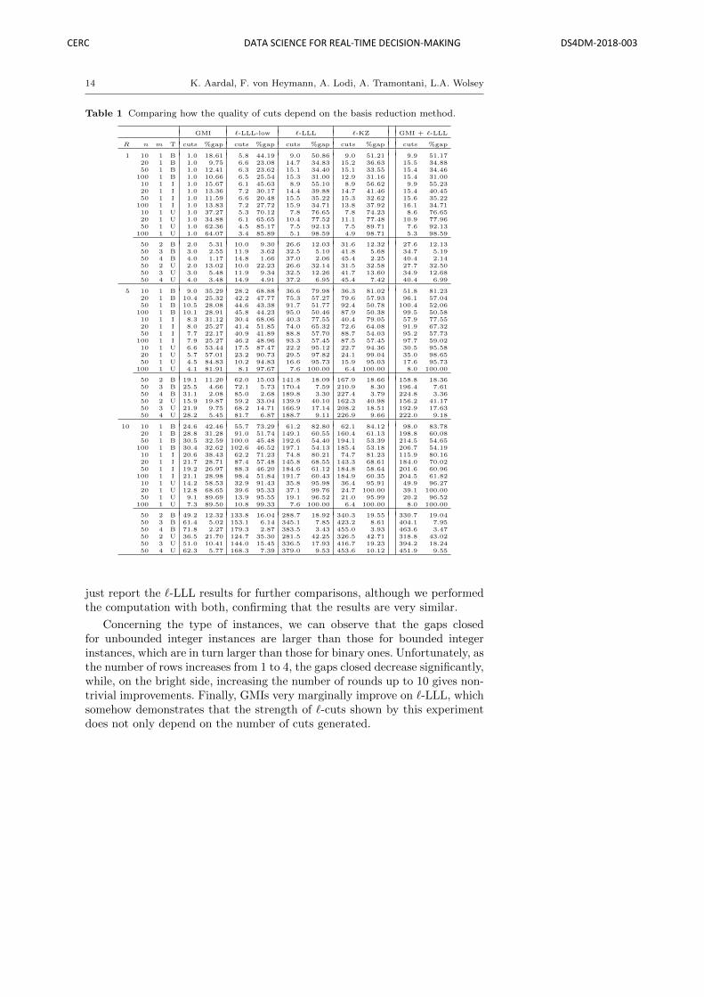
Table 1 reports on the results of the comparisons between: GMIs from theoptimal LP tableau, denoted by GMI, `-cuts from the reduction method LLL-low, denoted by `-LLL-low, `-cuts from the reduction method LLL, denotedby `-LLL, `-cuts from the reduction method KZ, denoted by `-KZ, and acombination of GMIs and `-LLL, denoted by GMI + `-LLL).

The other column headings are:R for the number of rounds of cuts, followedby n and m for the number of variables and constraints, respectively, and T forthe type of the instance. Then, for each approach, we report on the numberof cuts generated and the percentage of the gap that is closed between theoptimal LP and IP values, on average over 20 instances.

The results in Table 1 clearly show that the gap closed by `-cuts, indepen-dently of the basis reduction method, is significantly larger than that closed byonly using GMIs, but the number of cuts is much larger. Moreover, by using astrongly reduced lattice basis (`-LLL or `-KZ), we obtain a significantly largergap reduction than with a weaker reduction (`-LLL-low). The gaps closed forthe `-LLL and `-KZ reductions are not significantly different, typically varyingby less than 1%. As the LLL reduction is much cheaper to compute, we will



Table 1 Comparing how the quality of cuts depend on the basis reduction method.

GMI `-LLL-low `-LLL `-KZ GMI + `-LLL

R n m T cuts %gap cuts %gap cuts %gap cuts %gap cuts %gap

1 10 1 B 1.0 18.61 5.8 44.19 9.0 50.86 9.0 51.21 9.9 51.1720 1 B 1.0 9.75 6.6 23.08 14.7 34.83 15.2 36.63 15.5 34.8850 1 B 1.0 12.41 6.3 23.62 15.1 34.40 15.1 33.55 15.4 34.46

100 1 B 1.0 10.66 6.5 25.54 15.3 31.00 12.9 31.16 15.4 31.0010 1 I 1.0 15.67 6.1 45.63 8.9 55.10 8.9 56.62 9.9 55.2320 1 I 1.0 13.36 7.2 30.17 14.4 39.88 14.7 41.46 15.4 40.4550 1 I 1.0 11.59 6.6 20.48 15.5 35.22 15.3 32.62 15.6 35.22

100 1 I 1.0 13.83 7.2 27.72 15.9 34.71 13.8 37.92 16.1 34.7110 1 U 1.0 37.27 5.3 70.12 7.8 76.65 7.8 74.23 8.6 76.6520 1 U 1.0 34.88 6.1 65.65 10.4 77.52 11.1 77.48 10.9 77.9650 1 U 1.0 62.36 4.5 85.17 7.5 92.13 7.5 89.71 7.6 92.13

100 1 U 1.0 64.07 3.4 85.89 5.1 98.59 4.9 98.71 5.3 98.59

50 2 B 2.0 5.31 10.0 9.30 26.6 12.03 31.6 12.32 27.6 12.1350 3 B 3.0 2.55 11.9 3.62 32.5 5.10 41.8 5.68 34.7 5.1950 4 B 4.0 1.17 14.8 1.66 37.0 2.06 45.4 2.25 40.4 2.1450 2 U 2.0 13.02 10.0 22.23 26.6 32.14 31.5 32.58 27.7 32.5050 3 U 3.0 5.48 11.9 9.34 32.5 12.26 41.7 13.60 34.9 12.6850 4 U 4.0 3.48 14.9 4.91 37.2 6.95 45.4 7.42 40.4 6.99

5 10 1 B 9.0 35.29 28.2 68.88 36.6 79.98 36.3 81.02 51.8 81.2320 1 B 10.4 25.32 42.2 47.77 75.3 57.27 79.6 57.93 96.1 57.0450 1 B 10.5 28.08 44.6 43.38 91.7 51.77 92.4 50.78 100.4 52.06

100 1 B 10.1 28.91 45.8 44.23 95.0 50.46 87.9 50.38 99.5 50.5810 1 I 8.3 31.12 30.4 68.06 40.3 77.55 40.4 79.05 57.9 77.5520 1 I 8.0 25.27 41.4 51.85 74.0 65.32 72.6 64.08 91.9 67.3250 1 I 7.7 22.17 40.9 41.89 88.8 57.70 88.7 54.03 95.2 57.73

100 1 I 7.9 25.27 46.2 48.96 93.3 57.45 87.5 57.45 97.7 59.0210 1 U 6.6 53.44 17.5 87.47 22.2 95.12 22.7 94.36 30.5 95.5820 1 U 5.7 57.01 23.2 90.73 29.5 97.82 24.1 99.04 35.0 98.6550 1 U 4.5 84.83 10.2 94.83 16.6 95.73 15.9 95.03 17.6 95.73

100 1 U 4.1 81.91 8.1 97.67 7.6 100.00 6.4 100.00 8.0 100.00

50 2 B 19.1 11.20 62.0 15.03 141.8 18.09 167.9 18.66 158.8 18.3650 3 B 25.5 4.66 72.1 5.73 170.4 7.59 210.9 8.30 196.4 7.6150 4 B 31.1 2.08 85.0 2.68 189.8 3.30 227.4 3.79 224.8 3.3650 2 U 15.9 19.87 59.2 33.04 139.9 40.10 162.3 40.98 156.2 41.1750 3 U 21.9 9.75 68.2 14.71 166.9 17.14 208.2 18.51 192.9 17.6350 4 U 28.2 5.45 81.7 6.87 188.7 9.11 226.9 9.66 222.0 9.18

10 10 1 B 24.6 42.46 55.7 73.29 61.2 82.80 62.1 84.12 98.0 83.7820 1 B 28.8 31.28 91.0 51.74 149.1 60.55 160.4 61.13 198.8 60.0850 1 B 30.5 32.59 100.0 45.48 192.6 54.40 194.1 53.39 214.5 54.65

100 1 B 30.4 32.62 102.6 46.52 197.1 54.13 185.4 53.18 206.7 54.1910 1 I 20.6 38.43 62.2 71.23 74.8 80.21 74.7 81.23 115.9 80.1620 1 I 21.7 28.71 87.4 57.48 145.8 68.55 143.3 68.61 184.0 70.0250 1 I 19.2 26.97 88.3 46.20 184.6 61.12 184.8 58.64 201.6 60.96

100 1 I 21.1 28.98 98.4 51.84 191.7 60.43 184.9 60.35 204.5 61.8210 1 U 14.2 58.53 32.9 91.43 35.8 95.98 36.4 95.91 49.9 96.2720 1 U 12.8 68.65 39.6 95.33 37.1 99.76 24.7 100.00 39.1 100.0050 1 U 9.1 89.69 13.9 95.55 19.1 96.52 21.0 95.99 20.2 96.52

100 1 U 7.3 89.50 10.8 99.33 7.6 100.00 6.4 100.00 8.0 100.00

50 2 B 49.2 12.32 133.8 16.04 288.7 18.92 340.3 19.55 330.7 19.0450 3 B 61.4 5.02 153.1 6.14 345.1 7.85 423.2 8.61 404.1 7.9550 4 B 71.8 2.27 179.3 2.87 383.5 3.43 455.0 3.93 463.6 3.4750 2 U 36.5 21.70 124.7 35.30 281.5 42.25 326.5 42.71 318.8 43.0250 3 U 51.0 10.41 144.0 15.45 336.5 17.93 416.7 19.23 394.2 18.2450 4 U 62.3 5.77 168.3 7.39 379.0 9.53 453.6 10.12 451.9 9.55

just report the `-LLL results for further comparisons, although we performedthe computation with both, confirming that the results are very similar.

Concerning the type of instances, we can observe that the gaps closedfor unbounded integer instances are larger than those for bounded integerinstances, which are in turn larger than those for binary ones. Unfortunately, asthe number of rows increases from 1 to 4, the gaps closed decrease significantly,while, on the bright side, increasing the number of rounds up to 10 gives non-trivial improvements. Finally, GMIs very marginally improve on `-LLL, whichsomehow demonstrates that the strength of `-cuts shown by this experimentdoes not only depend on the number of cuts generated.



5.2 Comparing k-cuts and `-cuts

In this section, we compare the behaviour of `-cuts and k-cuts. More precisely,we separate k-cuts in the following two possible ways. For each tableau row,with basic variable, say, xj , we

1. multiply the row by an integer value k = 1, . . . , 10 and we thereby generate10 possibly different k-cuts,

2. multiply the row by an integer wij , i = 1, . . . , n−m, and we generate n−mpossibly different k-cuts.

In other words, we either use “trivial” values for k, or we use individual k’sfrom the reduced basis LLL. Note that, for the latter, k-cuts and `-cuts areidentical for the special case of R = 1 and m = 1, see Section 4.1.

Table 2 reports on the results of the comparisons among: GMIs from theoptimal LP tableau, denoted by GMI, k-cuts of type 1 above, denoted byk− 10, k-cuts of type 2 above, denoted by k-LLL, a combination of GMIs andk-cuts, denoted by GMI + k-LLL, `-cuts from LLL-reduced bases, denoted asbefore by `-LLL, and a combination of GMIs and `-LLL, denoted by GMI+`-LLL. (Note that columns GMI, `-LLL and GMI+`-LLL are the same as inTable 1.)

The results in Table 2 clearly show that for R > 1 the gap closed by `-LLL is significantly larger than that closed by k-LLL and with far fewer cuts.Recall that the entries for k-LLL and `-LLL are necessarily identical for R = 1and m = 1. Moreover, the gap closed by k-LLL is slightly larger than that ofk − 10, but with more cuts in general. Finally, the improvement of GMIs +k-LLL with respect to k-LLL is much more significant than that of GMIs +`-LLL with respect to `-LLL.

5.3 Comparing rank and row aggregation

In this section, we compare the use of `-cuts in multiple rounds, as in theprevious tables, i.e., by using for separation the row aggregation provided bythe simplex algorithm, with the case in which we optimize over the aggregationby solving an LP but we stay at rank 1, i.e., we only use the original constraintsand the W -matrix. The latter procedure, if iterated, allows to compute theapproximated strengthened `-LLL closure, by adapting the algorithm proposedby Bonami [8] for the strengthened lift-and-project closure. More precisely,

– The strengthened lift-and-project closure of a mixed integer linear programis the polyhedron obtained by intersecting all strengthened lift-and-projectcuts [5,18] obtained from its initial formulation, or equivalently all GMIsread from all tableaus corresponding to feasible and infeasible bases of theLP relaxation. An approximation of this closure is computed by iterativelygenerating lift-and-project cuts and strengthening them by integer lifting,see [8].



Table 2 Comparing k-cuts and `-cuts

GMI k − 10 k-LLL GMI + k-LLL `-LLL GMI + `-LLL

R n m T cuts %gap cuts %gap cuts %gap cuts %gap cuts %gap cuts %gap

1 10 1 B 1.0 18.61 10.0 34.46 9.0 50.86 9.9 51.17 9.0 50.86 9.9 51.1720 1 B 1.0 9.75 10.0 23.74 14.7 34.83 15.5 34.88 14.7 34.83 15.5 34.8850 1 B 1.0 12.41 10.0 26.83 15.1 34.40 15.4 34.46 15.1 34.40 15.4 34.46

100 1 B 1.0 10.66 10.0 29.40 15.3 31.00 15.4 31.00 15.3 31.00 15.4 31.0010 1 I 1.0 15.67 10.0 30.16 8.9 55.10 9.9 55.23 8.9 55.10 9.9 55.2320 1 I 1.0 13.36 10.0 30.92 14.4 39.88 15.4 40.45 14.4 39.88 15.4 40.4550 1 I 1.0 11.59 10.0 24.08 15.5 35.22 15.6 35.22 15.5 35.22 15.6 35.22

100 1 I 1.0 13.83 10.0 31.55 15.9 34.71 16.1 34.71 15.9 34.71 16.1 34.7110 1 U 1.0 37.27 9.8 66.25 7.8 76.65 8.6 76.65 7.8 76.65 8.6 76.6520 1 U 1.0 34.88 9.7 74.18 10.4 77.52 10.9 77.96 10.4 77.52 10.9 77.9650 1 U 1.0 62.36 7.4 87.95 7.5 92.13 7.6 92.13 7.5 92.13 7.6 92.13

100 1 U 1.0 64.07 5.6 98.71 5.1 98.59 5.3 98.59 5.1 98.59 5.3 98.59

50 2 B 2.0 5.31 19.7 10.11 50.0 12.87 50.9 12.87 26.6 12.03 27.6 12.1350 3 B 3.0 2.55 30.0 4.22 92.5 5.54 94.5 5.61 32.5 5.10 34.7 5.1950 4 B 4.0 1.17 40.0 2.17 139.7 2.51 142.9 2.53 37.0 2.06 40.4 2.1450 2 U 2.0 13.02 20.0 24.49 42.7 33.06 43.5 33.14 26.6 32.14 27.7 32.5050 3 U 3.0 5.48 30.0 11.20 87.9 13.41 89.9 13.58 32.5 12.26 34.9 12.6850 4 U 4.0 3.48 40.0 6.32 137.2 8.50 139.9 8.50 37.2 6.95 40.4 6.99

5 10 1 B 9.0 35.29 127.6 47.98 105.7 54.14 126.1 62.70 36.6 79.98 51.8 81.2320 1 B 10.4 25.32 156.1 33.03 235.8 37.52 266.2 45.44 75.3 57.27 96.1 57.0450 1 B 10.5 28.08 157.8 38.24 283.1 41.54 300.0 42.91 91.7 51.77 100.4 52.06

100 1 B 10.1 28.91 164.0 40.02 261.0 40.92 270.3 41.71 95.0 50.46 99.5 50.5810 1 I 8.3 31.12 122.9 42.23 140.5 56.14 145.2 64.05 40.3 77.55 57.9 77.5520 1 I 8.0 25.27 135.1 36.05 234.9 43.39 256.6 49.93 74.0 65.32 91.9 67.3250 1 I 7.7 22.17 132.9 32.33 236.3 42.28 243.4 44.61 88.8 57.70 95.2 57.73

100 1 I 7.9 25.27 138.9 39.05 254.2 42.27 262.0 43.13 93.3 57.45 97.7 59.0210 1 U 6.6 53.44 88.9 73.83 68.2 79.29 68.2 83.30 22.2 95.12 30.5 95.5820 1 U 5.7 57.01 77.8 84.04 98.7 81.13 103.0 87.07 29.5 97.82 35.0 98.6550 1 U 4.5 84.83 30.9 91.36 43.9 94.87 45.0 94.88 16.6 95.73 17.6 95.73

100 1 U 4.1 81.91 12.8 100.00 16.2 100.00 15.9 100.00 7.6 100.00 8.0 100.00

50 2 B 19.1 11.20 244.3 13.47 675.0 15.27 711.1 15.98 141.8 18.09 158.8 18.3650 3 B 25.5 4.66 320.6 5.80 1072.4 6.43 1104.2 6.79 170.4 7.59 196.4 7.6150 4 B 31.1 2.08 372.8 2.79 1439.8 2.74 1472.2 2.97 189.8 3.30 224.8 3.3650 2 U 15.9 19.87 225.0 28.63 654.0 36.15 663.0 36.99 139.9 40.10 156.2 41.1750 3 U 21.9 9.75 314.9 13.29 1032.3 14.76 1031.1 15.97 166.9 17.14 192.9 17.6350 4 U 28.2 5.45 358.6 7.39 1432.1 8.93 1495.8 9.51 188.7 9.11 222.0 9.18

10 10 1 B 24.6 42.46 301.9 52.21 223.9 54.93 300.7 65.92 61.2 82.80 98.0 83.7820 1 B 28.8 31.28 359.9 37.12 510.0 38.10 645.3 47.84 149.1 60.55 198.8 60.0850 1 B 30.5 32.59 397.3 40.99 637.5 43.25 688.2 45.17 192.6 54.40 214.5 54.65

100 1 B 30.4 32.62 398.8 42.82 600.7 44.02 624.3 44.82 197.1 54.13 206.7 54.1910 1 I 20.6 38.43 269.6 44.70 285.8 56.77 318.5 65.69 74.8 80.21 115.9 80.1620 1 I 21.7 28.71 308.3 37.71 499.9 44.22 551.8 52.77 145.8 68.55 184.0 70.0250 1 I 19.2 26.97 320.5 34.75 515.2 43.31 532.9 46.65 184.6 61.12 201.6 60.96

100 1 I 21.1 28.98 326.8 43.72 536.0 43.22 541.4 45.74 191.7 60.43 204.5 61.8210 1 U 14.2 58.53 183.3 76.06 143.6 80.54 143.3 85.03 35.8 95.98 49.9 96.2720 1 U 12.8 68.65 158.7 87.45 212.3 82.67 212.2 89.62 37.1 99.76 39.1 100.0050 1 U 9.1 89.69 63.3 92.12 77.9 94.98 75.7 95.04 19.1 96.52 20.2 96.52

100 1 U 7.3 89.50 12.8 100.00 16.2 100.00 15.9 100.00 7.6 100.00 8.0 100.00

50 2 B 49.2 12.32 573.2 14.08 1486.7 15.69 1580.3 16.62 288.7 18.92 330.7 19.0450 3 B 61.4 5.02 726.6 6.05 2227.4 6.64 2318.9 6.98 345.1 7.85 404.1 7.9550 4 B 71.8 2.27 847.6 2.90 2895.1 2.84 3035.1 3.07 383.5 3.43 463.6 3.4750 2 U 36.5 21.70 486.8 29.71 1323.9 36.65 1360.1 38.22 281.5 42.25 318.8 43.0250 3 U 51.0 10.41 672.9 13.75 2102.6 14.95 2118.5 16.26 336.5 17.93 394.2 18.2450 4 U 62.3 5.77 760.1 7.64 2812.4 9.00 2960.1 9.65 379.0 9.53 451.9 9.55

– Analogously, given a reduced W -matrix to generate rank-1 `-cuts, the ap-proximated strengthened `-LLL closure is computed as follows. If x∗ isthe optimal LP solution and wix∗ /∈ Z, one generates an intersection cut[5] on the disjunction, wix ≤ bwix∗c and wix ≥ dwix∗e, which is thenstrengthened. This is repeated for each row i of W at each iteration untilno more violated cuts are found.

In terms of closures, the comparison is completed by reporting on the results forthe split closure. Exploiting the result reported [17] that shows the equivalencebetween the split closure and the Mixed-Integer Rounding (MIR) closure, thesplit closure is computed by iteratively separating violated MIR cuts throughthe solution of a mixed-integer program as in [17].

Table 3 reports on the results on the comparisons between:



– 10 rounds of: (a) `-LLL cuts, (b) a combination of GMIs and `-LLL cuts,denoted by GMI+`-LLL, and

– the approximated closures of: (c) strengthened lift-and-project cuts, de-noted by “str. L&P”, (d) strengthened `-LLL cuts, denoted by “str. `-LLL”,(e) split cuts, denoted by “split”.

In contrast to the cases of strengthened L&P and `-LLL closures, the term“approximated” for the split closure refers to the fact that the computationis stopped after a time limit of 5 hours. Such a time limit affects only themulti-row instances with binary variables and this is indicated in the table by“*”.

Table 3 Comparing higher rank cuts with rank-1 closures

10 rounds “approximated” closures

`-LLL GMI + `-LLL str. L&P str. `-LLL split

n m T cuts %gap cuts %gap cuts %gap cuts %gap cuts %gap

10 1 B 61.2 82.80 98.0 83.78 4.1 29.87 41.6 99.73 62.3 100.0020 1 B 149.1 60.55 198.8 60.08 4.0 18.56 71.4 61.93 148.4 84.1150 1 B 192.6 54.40 214.5 54.65 4.1 22.32 48.0 50.84 174.7 88.29

100 1 B 197.1 54.13 206.7 54.19 4.4 21.38 42.8 46.81 162.3 89.7210 1 I 74.8 80.21 115.9 80.16 1.3 16.89 14.3 63.87 48.3 88.9720 1 I 145.8 68.55 184.0 70.02 1.3 13.68 21.2 47.42 53.9 81.9050 1 I 184.6 61.12 201.6 60.96 1.2 12.26 21.1 42.02 61.6 82.28

100 1 I 191.7 60.43 204.5 61.82 1.3 14.94 20.2 42.28 57.0 85.2210 1 U 35.8 95.98 49.9 96.27 1.0 37.27 8.8 79.31 25.9 97.5820 1 U 37.1 99.76 39.1 100.00 1.0 34.88 10.4 77.52 27.0 92.5750 1 U 19.1 96.52 20.2 96.52 1.0 62.36 7.5 92.13 38.1 99.97

100 1 U 7.6 100.00 8.0 100.00 1.0 64.07 5.1 98.59 35.9 98.70

50 2 B 288.7 18.92 330.7 19.04 10.1 9.95 84.4 18.96 460.8 41.24 *50 3 B 345.1 7.85 404.1 7.95 15.8 4.23 99.7 8.09 519.0 18.95 *50 4 B 383.5 3.43 463.6 3.47 20.7 1.99 140.5 4.05 518.6 8.49 *50 2 U 281.5 42.25 318.8 43.02 2.0 13.02 26.7 32.28 178.6 71.8750 3 U 336.5 17.93 394.2 18.24 3.3 5.57 34.7 12.81 342.4 42.0850 4 U 379.0 9.53 451.9 9.55 4.7 3.76 40.9 7.49 372.8 22.41

The results in Table 3 clearly show that growing the rank of the `-cutsgives generally better results than optimizing over the approximate closureof the disjunctions in the W -matrix although there is no domination. Nev-ertheless, it is confirmed that the approximated strengthened `-LLL closureis way stronger than the approximated strengthened L&P closure. In otherwords, elementary disjunctions in the reformulated space are stronger than el-ementary disjunctions in the original space. With few exceptions, neither thestrengthened `-LLL closure nor the strengthened L&P closure provide a goodapproximation of the rank-1 split closure. Finally, separating both `-LLL andL&P cuts together does not significantly improve over `-LLL alone, althoughthe results are not explicitly reported in the table.



6 Concluding remarks

Our `-cuts are generated based on general disjunctions originating from in-formation on the lattice structure of the underlying problem. For the test in-stances, which are similar to the instances used by [14] in their computationalstudy of k-cuts, we observe that the lattice structure gives useful informa-tion to obtain cuts that improve on standard GMI/Split cuts and k-cuts. Forsingle-row problems, a large percentage of the integrality gap is closed. Formulti-row problems the results are not as good, and it remains a challengeto identify cuts that can be generated within reasonable computing time andthat work well on multi-row problems.

We observe that the better the quality of the basis generating the lattice,the better the quality of the resulting `-cuts. We have, however, only tried onelattice reformulation [1], and given the partial success of the approach it wouldbe useful to investigate other reformulations, in particular a reformulationthat captures multi-row problems better. Also, extending our approach to themixed-integer case would be interesting.

References

1. Aardal, K., Hurkens, C.A.J., Lenstra, A.K.: Solving a system of linear Diophantineequations with lower and upper bounds on the variables. Mathematics of OperationsResearch 25(3), 427–442 (2000).

2. Aardal, K., Lenstra, A.K.: Hard equality constrained integer knapsacks. Mathemat-ics of Operations Research 29(3), 724–738 (2004). Erratum: Mathematics of OperationsResearch 31(4), 846 (2006).

3. Aardal, K., Bixby, R.E., Hurkens, C.A.J., Lenstra, A.K., Smeltink, J.W.: Market splitand basis reduction: Towards a solution of the Cornuejols-Dawande instances. INFORMSJournal on Computing 12, 192–202 (2000).

4. Aardal, K., Wolsey, L.A.: Lattice based extended formulations for integer linear equalitysystems. Mathematical Programming 121, 337–352 (2010).

5. Balas, E.: Intersection cuts—a new type of cutting planes for integer programming. Op-erations Research 19, 19–39 (1971).

6. Balas, E., Saxena, A.: Optimizing over the split closure. Mathematical Programming113(2), 219–240 (2008).

7. Bixby, R.E., Gu, Z., Rothberg, E., Wunderling, R.: Mixed integer programming: Aprogress report. In: Grotschel, M. (ed.), The Sharpest Cut: The Impact of Manfred Pad-berg and His Work, MPS/SIAM Series in Optimization, 309–326 (2004).

8. Bonami, P.: On optimizing over lift-and-project closures. Mathematical ProgrammingComputation 4(2), 151–179 (2012).

9. Caprara, A., Letchford, A.N.: On the separation of split cuts and related inequalities.Mathematical Programming 94, 279–294 (2006).

10. Chvatal, V.: Edmonds polytopes and a hierarchy of combinatorial problems. DiscreteMathematics 4, 305–337 (1973).

11. Conforti, M., Cornuejols, G., Zambelli, G.: Integer Programming. Springer (2014).12. Cook, W., Kannan, R., Schrijver, A.: Chvatal closures for mixed-integer programming.

Mathematical Programming 47, 155–174 (1990).13. Cornuejols, G.: Valid inequalities for mixed integer linear programs. Mathematical Pro-

gramming 112, 3-44 (2008).14. Cornuejols, G., Li, Y., Vandenbusche, D.: K-cuts: A variation of Gomory Mixed Integer

Cuts from the LP tableau. INFORMS Journal on Computing 15(4), 385–396 (2003).



15. Cornuejols, G., Nannicini, G.: Practical strategies for generating rank-1 split cuts inmixed-integer linear programming. Mathematical Programming Computation 3(4), 281–318 (2011).

16. Dash, S., Goycoolea, M.: A heuristic to generate rank-1 GMI cuts. Mathematical Pro-gramming Computation 2, 231–257 (2010).

17. Dash, S., Gunluk, O., Lodi, A.: MIR closures of polyhedral sets, Mathematical Pro-gramming 121, 33–60 (2010).

18. Fischetti, M., Lodi, A., Tramontani, A.: On the separation of disjunctive cuts. Mathe-matical Programming 128, 205–230 (2011).

19. Fischetti, M. Salvagnin, D.: A relax-and-cut framework for Gomory mixed-integer cuts.Mathematical Programming Computation 3, 79–102 (2011).

20. Gomory, R.E.: An algorithm for integer solutions to linear programs. In: Graves, R.L.,Wolfe, P. (eds.), Recent Advances in Mathematical Programming, McGraw-Hill, NewYork, NY, 269–302 (1963).

21. Gomory, R.E.: Some polyhedra related to combinatorial problems. Linear Algebra andIts Applications 2, 451–558 (1969).

22. von Heymann, F.: On Lattice Methods in Integer Optimization. PhD Thesis, DelftUniversity of Technology, ISBN 978-94-6191-874-1 (2013).

23. Korkine, A., Zolotareff, G.: Sur les formes quadratiques. Mathematische Annalen 6,366–389 (1873).

24. Lagarias, J.C., Lenstra, Jr., H.W., Schnorr, C.P.: Korkin-Zolotarev bases and successiveminima of a lattice and its reciprocal lattice. Combinatorica 10(4), 333–348 (1990).

25. Lenstra, A.K., Lenstra, Jr., H.W., Lovasz, L.: Factoring polynomials with rationalcoefficients. Mathematische Annalen 261(4), 515–534 (1982).

26. Mehrotra, S., Li, Z.: Branching on hyperplane methods for mixed integer linear andconvex programming using adjoint lattices. Journal of Global Optimization 49(4), 623–649(2011).

27. Nemhauser, G.L., Wolsey, L.A.: Integer and Combinatorial Optimization. Wiley-Interscience, New York, NY (1988).

28. Nemhauser, G.L., Wolsey, L.A.: A recursive procedure to generate all cuts for 0-1 mixedinteger programs. Mathematical Programming 46, 379–390 (1990).

29. Schrijver, A.: Theory of Linear and Integer Programming. John Wiley & Sons Ltd.(1986).


Technical Report - Polytechnique Montréal

Documents

Transcript of Technical Report - Polytechnique Montréal