Technical Report - CGSpace · PDF file(GTS). Once in the GTS ... This section provides an...
97
Technical Report: Observations and reanalyses data: comparison and trends in Southeast Asia Richard Washington Helen Pearce Sebastian Engelstaedter Thien-Kim Diep Climate Research Lab University of Oxford January 2014
Transcript of Technical Report - CGSpace · PDF file(GTS). Once in the GTS ... This section provides an...

Technical Report:
Observations and reanalyses data: comparison and trends in Southeast Asia
Richard Washington
Helen Pearce
Sebastian Engelstaedter
Thien-Kim Diep
Climate Research Lab
University of Oxford
January 2014

2
1 Part 1: Observations and reanalyses data: comparison and trends
Reanalyses data sets, being temporally and spatially complete and available on six hourly
timescales, are extremely convenient to use. Real observations represent the climate system with
greater fidelity than reanalyses can, given that the latter are a complicated blend of observations and
models via an assimilation scheme and rely heavily on the assimilation scheme where observations
are absent. Knowing whether the reanalyses data reflects real data can be difficult to establish. In
this part of the report, the observed data is compared with three reanalyses data sets for the SE Asia
region. We use observations from SYNOP and METAR reports. SYNOP and METAR data are, in
effect, observations taken at met stations and delivered to the Global Telecommunication System
(GTS). Once in the GTS, they can be archived by institutions such as those delivering weather
forecasts. Access to these data via the archives is generally much easier than through the individual
Met Agencies. This is particularly true in the case of a study covering multiple nation states. These
datasets are described in more detail in Sections 1.1 and 1.2.
1.1 Methods
This section provides an overview of the data and data processing.
Surface observations and data processing
Basic measurements made at meteorological stations all over the world are distributed through
surface synoptic observations (SYNOP) and météorologique aviation régulière (METAR) reports.
SYNOP reports generally include more variables than the METAR reports which are distributed
primarily for the aviation industry. The UK Meteorological Office compiled SYNOP and METAR
reports in the Met Office Integrated Data Archive System (MIDAS) Land and Marine Surface
Stations Data (1853-present) archive. We use data from the MIDAS Global Weather Observations
(GL) table which includes 3-hourly observations from global non-UK stations from 1974 to present
(http://badc.nerc.ac.uk/data/ukmo-midas/GL_Table.html).
The observation period, as well as the frequency of observations, varies significantly between
stations and may vary significantly over time. Basic quality control is performed by the observer at
each station before the data are transmitted as SYNOP or METAR reports. Before the data are

3
included in the MIDAS archive, they undergo a range of quality checks outlined in the 'Met Office
Surface Data User Guide' Section 7 (http://badc.nerc.ac.uk/data/ukmo-midas/ukmo_guide.html).
In order to derive a consistent, quality assured dataset, the SYNOP and METAR data were further
processed in the following way. At stations where observations from both SYNOP and METAR
reports were available for the same observation time, the observations from the SYNOP report were
used in preference to METAR because SYNOP observations are more frequent then METAR
observations (thereby keeping the dataset as consistent as possible). Gaps in the SYNOP
observation times were substituted by METAR observations where possible to make observations
as complete as possible. Although for some stations 3-hourly observations are available, we only
use observations made at the synoptic hours (00, 06, 12 and 18 UTC). All mean sea-level pressure
(MSLP), air temperature at 2m (T2m) and wind speed at 10m (WSPD10m) observations between 1
January 1989 00:00 UTC and 31 December 2009 18:00 UTC were extracted.
Reanalyses (ERAI, CFSR and MERRA)
Surface observations from SYNOP/METAR of mean sea-level pressure, air temperature at 2m and
wind speed at 10m are compared with the corresponding fields of three reanalysis datasets. For this
comparison, fields for three reanalysis datasets were obtained in 6-hourly time steps (00, 06, 12 and
18 UTC) between 1 January 1989 and 12 December 2009. This 21 year period was chosen because
all three reanalyses are available for this period.
European Centre for Medium-Range Weather Forecasts (ECMWF) interim reanalysis (ERAI) [Dee
et al., 2011] full resolution global fields were obtained from the ECMWF website (http://data-
portal.ecmwf.int/data/d/interim_full_daily). The fields are available in netCDF format and in
0.703125° by 0.703125° spatial resolution. For the trend analysis, the MSLP, T2m, WSPD10m and
total precipitation fields were obtained for the whole ERA-Interim period 1 January 1979 to 31
December 2012. Whereas MSLP, T2m and WSPD10m are available as reanalysis fields, total
precipitation is only available as 3-hourly forecast fields with forecasts being initialised at 00 and
12 UTC every day.

4
A subset of the reanalysis domain covering SE Asia was extracted from the National Aeronautics
and Space Administration (NASA) modern-era retrospective analysis for the research and
applications (MERRA) dataset [Rienecker et al., 2011] and was obtained from the Goddard Earth
Sciences Data and Information Services Center (GES DISC) website
(http://disc.sci.gsfc.nasa.gov/daac-bin/FTPSubset.pl). We use the SLP (Sea level pressure), T2M
(Temperature at 2m above the displacement height) and U10M/V10M (Eastward/Northward wind
at 10m above displacement height) fields of the 'IAU 2d atmospheric single-level diagnostics
(tavg1_2d_slv_Nx)' product. The fields are available in netCDF format and come in a 2/3°
longitude by 0.5° latitude resolution.
The National Centers for Environmental Prediction (NCEP) Climate Forecast System Reanalysis
(CFSR) fields [Suranjana et al., 2010] for MSLP, air temperature at 2m as well as U and V wind
components at 10m were obtained through the National Oceanic and Atmospheric Administration
(NOAA) National Operational Model Archive & Distribution System (NOMADS,
ftp://nomads.ncdc.noaa.gov/CFSR/HP_time_series/). The MSLP field is available at a resolution of
0.5° by 0.5° whereas the 2m air temperature and 10m wind speed fields are 0.3125° by 0.3125°.
Station selection and minimum data availability thresholds
There are normally many missing variables in the SYNOP/METAR data set and the number of
observations available for the period 1989 to 2009 varies between stations, synoptic hours and
variables. In order to deal with this, a minimum data availability threshold of 400 observations over
the record 1989-2009 was chosen for a station to be included in this analysis. For the analysis of the
seasonal statistics, this threshold was lowered to a quarter of 400 (n=100). These thresholds were
chosen as a compromise that allows a large enough sample for statistical analysis while maintaining
a reasonably good spatial coverage.
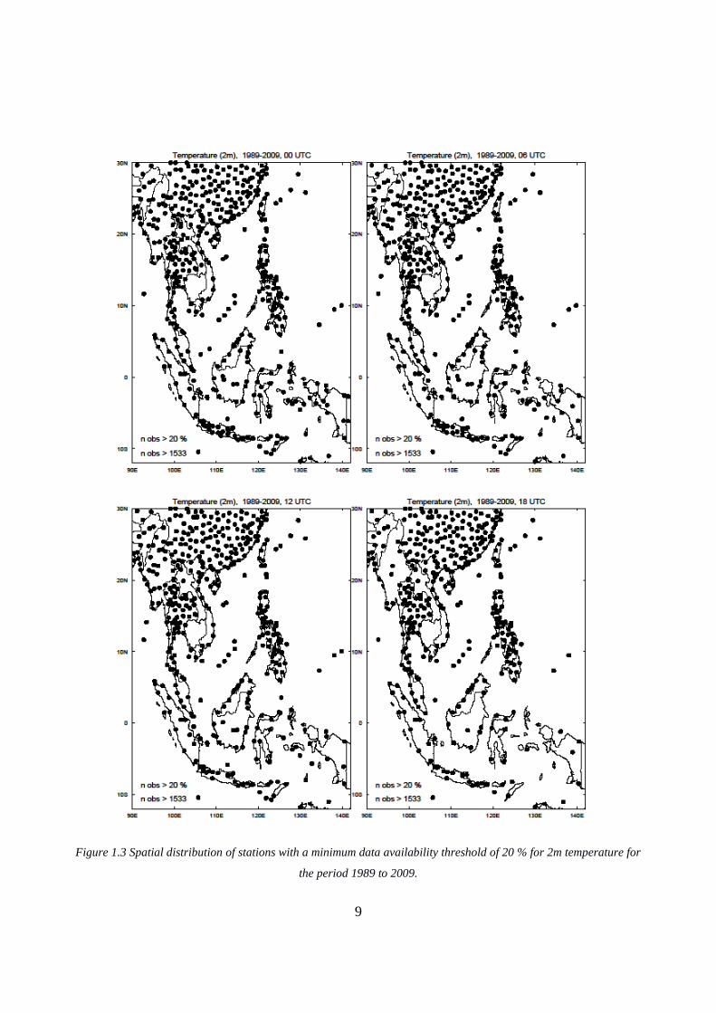
Figures 1.1 to 1.6 show the spatial distribution of stations with T2m measurements for each
synoptic hour when thresholds of 6 (n=460), 10 (n=767), 20 (n=1533), 30 (n=2300), 40 (n=3066)
and 50% (n=3833) minimum data availability are applied, respectively. The relatively low
minimum data availability threshold of 400 observations was chosen so that Cambodia and western
Indonesia (Papua) are represented in the analysis. Cambodia is the country with the least number of

5
observations (<500). The 400 observations threshold is justifiable because when comparing the
station availability for the different thresholds (Figures 1.1 to 1.6), it becomes evident that
increasing the threshold to 20% does not significantly change the station distribution apart from
over Cambodia and for one station in the centre of Papua, Indonesia. Only for thresholds larger than
20% (e.g., 30, 40 and 50%, Figure 1.4, 1.5 and 1.6) do larger gaps in the station availability become
apparent, especially in Indonesia.

6
Figure 1.1 Spatial distribution of stations with a minimum data availability threshold of 6% for 2m temperature for the
period 1989 to 2009

7

8
Figure 1.2 Spatial distribution of stations with a minimum data availability threshold of 10% for 2m temperature for
the period 1989 to 2009.
9
Figure 1.3 Spatial distribution of stations with a minimum data availability threshold of 20 % for 2m temperature for
the period 1989 to 2009.

10
Figure 1.4 Spatial distribution of stations with a minimum data availability threshold of 30 % for 2m temperature for
the period 1989 to 2009.

11
Figure 1.5 Spatial distribution of stations with a minimum data availability threshold of 40 % for 2m temperature for
the period 1989 to 2009.

12
Figure 1.6 Spatial distribution of stations with a minimum data availability threshold of 50 % for 2m temperature for
the period 1989 to 2009.

13
The distribution of stations for observations at 00, 06 and12 UTC are very similar (e.g., Figure 1.1).
The number of stations available for statistical analysis drops, however, for observations made at 18
UTC which corresponds to night time in the South-East Asia domain. See the end of this section for
a brief discussion of time zones. The number of stations available for analysis does not vary
significantly between the different variables (not shown).
As the stations will have different numbers of observations, a meaningful comparison of their
climatology is difficult. To overcome this problem we extract 400 random samples from the record
of each station and calculate means based on them. To avoid the chance of accidentally poor
sampling, we repeat the extraction of 400 random samples 100 times. The 100 means will be
Gaussian distributed around the ‘true’ mean of the station. Therefore, calculating the mean of them
will give a more realistic representation of the climatology while still maintaining the same sample
size at each station.
Reanalyses comparison
The SYNOP/METAR observations are compared with the ERA-Interim, CFSR and MERRA
reanalysis products. The following approach was taken for the comparison. For each observation
used from the SYNOP/METAR data, the corresponding reanalysis value was extracted by
interpolating the gridded reanalysis field to the location of the observing station using bilinear
interpolation. Repeating this process created a record that has the same number of reanalysis values
as the observations allowing for a one-to-one comparison of the observations and the reanalysis.
Climatological means were calculated using the same approach as for the observations using the
same set of random indices as generated for each of the stations.
Spatial interpolation
The climatological means calculated at each station for the observations as well as all three
reanalyses have been interpolated spatially using linear interpolation.
Trend analysis
The ERA-Interim reanalysis is used to identify trends in climate data between 1979 and 2012 for

14
the SE Asia domain. Trends in climate extremes (5th and 95th percentile), as well as the mean, are
analysed for MSLP, T2m, WSPD10m and total precipitation.
For the trend analysis of the percentiles, daily MSLP, T2m and WSPD10m means were calculated
from the 6-hourly values for the whole period 1979-2012. Based on the daily mean values, the 5th
and 95th percentile was calculated for each year as well as for each season (DJF, MAM, JJA, JAS
and SON) yielding a time series of 34 values for each grid box. For precipitation the same approach
was taken but totals were calculated instead of means. A simple linear regression model was used to
calculate the slope of the regression line.
For the trend analysis of the monthly means, data were computed from daily means (based on 6-
hourly values). From the monthly means annual and seasonal (DJF, MAM, JJA, JAS and SON)
means were computed yielding a time series of 34 values for each grid box. Regression was
computed in the same way as for the percentile trend analysis described above.
Notes on time zones
The geographical domain covers four time zones spanning from UTC+6.5 to UTC+9. The times of
observations in the MIDAS dataset as well as the availability of the reanalysis products are 00, 06,
12 and 18 UTC. It is important to keep the relationship between observation times at the synoptic
hours and local time in mind when interpreting the climatological plots for specific synoptic hours.
Table 1.1 shows the relationship between UTC and local time.

15
Table 1.1: Relationship between GMT and local time
1.2 Analysis of observations: climatology
This section shows the baseline climatology of the region derived from observations (using linear
interpolation) for the annual mean (Figure 1.7) and each season DJF, MAM, JJA, JAS and SON
(Figures 1.8 to 1.12). In each case the climatology is shown for six hourly times (00, 06, 12, 18
UTC) and therefore resolves the diurnal cycle.
Peak long term annual mean observed temperatures are in Thailand. Topographic effects are evident
for isolated stations in Myanmar (2 stations at 12 UTC), Sumatra (1 station at 00 UTC) and Papua
(2 stations show much lower T2m).
Wind speed maxima occurs at 06 UTC (daytime) and minima at 18 and 00 UTC (night time).
Strong winds are found along the Vietnamese cost, mainland Malaysia, Java, Sulawesi and Sumatra,
especially during the daytime. Generally low winds occur in Myanmar and Thailand. Strong winds
GMT, UTC+0 UTC+6.5 UTC+7 UTC+8 UTC+9
Myanmar Laos, Thailand,
Cambodia,
Vietnam
Malaysia,
Philippines,
western Indonesia
eastern Indonesia
00 UTC 6:30am 7am 8am 9am
06 UTC 12:30pm 1pm 2pm 3pm
12 UTC 6:30pm 7pm 8pm 9pm
18 UTC 12:30am 1am 2am 3am

16
are found at a single station in Laos at 06 UTC (which is likely a local control). Coastal stations
show in general higher winds.
Mean annual sea level pressure (MSLP) generally decreases from north to south in DJF and
reverses in JJA consistent with the monsoon regime which dominates the area. Lowest MSLP
occurs in Myanmar in JJA.
As expected, surface temperature (T2m) peaks at 06 UTC although the T2m spatial distribution and
values are similar at 00 and 18 UTC. Temperature differences between seasons are small but DJF
emerges as the hottest season. Colder temperatures in central Papua reflect topography; there are
similar effects at other stations.

17
Figure 1.7 1989-2009 long term mean climatology of observed MSLP, T2m and WSPD for 00, 06, 12 and 18 UTC
employing linearly interpolated between stations.

18
Figure 1.8 1989-2009 long term seasonal mean climatology for DJF of observed MSLP, T2m and WSPD for 00, 06, 12
and 18 UTC employing linearly interpolated between stations.

19
Figure 1.9 1989-2009 long term seasonal mean climatology for MAM of observed MSLP, T2m and WSPD for 00, 06,
12 and 18 UTC employing linearly interpolated between stations.

20
Figure 1.10 1989-2009 long term seasonal mean climatology for JJA of observed MSLP, T2m and WSPD for 00, 06, 12
and 18 UTC employing linearly interpolated between stations.

21
Figure 1.11 1989-2009 long term seasonal mean climatology for JAS of observed MSLP, T2m and WSPD for 00, 06, 12
and 18 UTC employing linearly interpolated between stations.

22
Figure 1.12 1989-2009 long term seasonal mean climatology for SON of observed MSLP, T2m and WSPD for 00, 06,
12 and 18 UTC employing linearly interpolated between stations.

23
1.3 Comparison with reanalysis products
This section compares reanalyses with observations. In subsequent sections, trend analysis is
applied to the reanalyses data and global climate models are compared with reanalyses. Therefore it
is useful to establish the bias evident in reanalyses products.
MSLP
Figure 1.13 shows the reanalyses annual mean MSLP from the three reanalyses compared in this
study. Figure 1.14 shows the reanalysis minus the observed. CFSR and ERAI are similar with both
models overestimating MSLP apart from over Borneo and mainland Malaysia. MERRA shows a
somewhat different picture, mainly under prediction at 00, 06 and 18 UTC and over prediction at 12
UTC (evening).
T2m
Figure 1.15 shows the reanalyses annual mean T2m from the three reanalyses compared in this
study. Figure 1.16 shows the reanalysis minus the observed. All three reanalyses underestimate
T2m during daytime. The strongest underestimate is for continental countries at 12 UTC. During
night time a mixed pattern emerges with ERAI and MERRA overestimating T2m at many stations
in Sumatra, Java, Borneo and mainland Malaysia. Overall, all three reanalyses are similar.
WSPD
Figure 1.17 shows the reanalyses annual mean T2m from the three reanalyses compared in this
study. Figure 1.18 shows the reanalysis minus the observed. Spatial distribution of over and
underestimation are similar for all reanalyses although the magnitude varies. CFSR is closest to
observations. The largest underestimation of winds is during daytime (06 UTC) in non-continental
countries.

24
Figure 1.13 1989-2009 CFSR, ERAI and MERRA long term mean reanalysis MSLP for 00, 06, 12 and 18 UTC linearly
interpolated between stations.

25
Figure 1.14 1989-2009 reanalysis (CFSR, ERAI and MERRA) minus observed MSLP 00, 06, 12 and 18 UTC linearly
interpolated between stations.

26
Figure 1.15 1989-2009 CFSR, ERAI and MERRA long term mean reanalysis T2m for 00, 06, 12 and 18 UTC linearly
interpolated between stations.

27
Figure 1.16 1989-2009 reanalysis (CFSR, ERAI and MERRA) minus observed T2m 00, 06, 12 and 18 UTC linearly
interpolated between stations.

28
Figure 1.17 1989-2009 CFSR, ERAI and MERRA long term mean reanalysis WSPD10m for 00, 06, 12 and 18 UTC
linearly interpolated between stations.

29
Figure 1.18 1989-2009 reanalysis (CFSR, ERAI and MERRA) minus observed WSPD10m 00, 06, 12 and 18 UTC
linearly interpolated between stations.

30
Seasonal mean climatologies are included in the following figures for reference, which are found in
the Appendix.
MSLP
DJF: Figure 1.19 (reanalyses) and Figure 1.20 (reanalyses minus obs)
MAM: Figure 1.21 (reanalyses) and Figure 1.22 (reanalyses minus obs)
JJA: Figure 1.23 (reanalyses) and Figure 1.24 (reanalyses minus obs)
JAS: Figure 1.25 (reanalyses) and Figure 1.26 (reanalyses minus obs)
SON: Figure 1.27 (reanalyses) and Figure 1.28 (reanalyses minus obs)
T2m
DJF: Figure 1.29 (reanalyses) and Figure 1.30 (reanalyses minus obs)
MAM: Figure 1.31 (reanalyses) and Figure 1.32 (reanalyses minus obs)
JJA: Figure 1.33 (reanalyses) and Figure 1.34 (reanalyses minus obs)
JAS: Figure 1.35 (reanalyses) and Figure 1.36 (reanalyses minus obs)
SON: Figure 1.37 (reanalyses) and Figure 1.38 (reanalyses minus obs)
WSPD10m
DJF: Figure 1.39 (reanalyses) and Figure 1.40 (reanalyses minus obs)
MAM: Figure 1.41 (reanalyses) and Figure 1.42 (reanalyses minus obs)
JJA: Figure 1.43 (reanalyses) and Figure 1.44 (reanalyses minus obs)
JAS: Figure 1.45 (reanalyses) and Figure 1.46 (reanalyses minus obs)
SON: Figure 1.47 (reanalyses) and Figure 1.48 (reanalyses minus obs)
1.4 Trend analysis
Warming in SEA has been similar to the global mean warming (Cruz et al, 2007) with mean
temperature increasing across South-East Asia since the 1960s at a rate of up to 0.2ºC/decade
(Tangang et al, 2007).. Extreme rainfall and temperature are thought to have a greater impact on
crop cultivation than mean climate. In this respect, there is also a reported increase in the frequency
hot days/warm nights since the mid-20th
century (Caesar et al, 2011; Manton et al, 2001). Strongest
changes are found in the northern regions of SEA in particular, Thailand and Malaysia (Choi et al,
2009). This suggests the role of local variations in warming, especially the tendency for stronger

31
warming over landmass interiors than coastal regions (McGregor and Dix, 2001). Also, present
trends in surface air temperature are more pronounced in winter than in summer (Cruz et al, 2007).
Manton et al (2001) note that whilst generally rainfall has decreased over South-East Asia between
1961 and 1998, the trend is not statistically significant. Nonetheless, some significant trends were
found, notably, a statistically significant decrease in the number of rain days over much of the
domain was found. More recently, other authors have found additional trends in South-East Asian
rainfall. Lau and Wu (2007) suggest that moderate rainfall events have been decreasing in
occurrence, with an increase in the amount of heavy and light rainfall events, measuring in the top
10% and bottom 5% of events respectively.
The analysis undertaken above shows less frequent and more intense precipitation for tropical
regions, as evident in the HadEX2 dataset (Donat et al, 2013) and other observations (Yao et al,
2010). A strong increase in extreme precipitation is found between 1951-2010 across all seasons
and the number of days with at least 2mm of rain has decreased (Manton et al, 2001); although
responses are regionally variable (Choi et al, 2009; Donat et al, 2013).
Individual regions of South-East Asia have also seen climatic trends. It has been suggested that
there is a decreasing trend in extreme rainfall events in Myanmar (Chang, 2011). This contrasts to
the trend over much of the northern region of the domain where extreme events have been
increasing in frequency. A further regional example is peninsular Malaysia, with contrasting trends
seen in total rainfall between the northeast and southwest monsoon seasons. During the northeast
monsoon, total rainfall was found to have increased (Suhaila et al, 2010), but in contrast during the
southwest monsoon a decrease in total rainfall has been established, despite an increase in intensity
of rainfall events (Deni et al, 2010). For Indonesia, a contrast in rainfall trends between seasons has
also been found, with Aldrian and Djamil, 2008) suggesting that there has been an increase in the
ratio of rainfall of the wet to dry season.
For this report, trends are computed based on ERA-I reanalysis. Annual trends are discussed first,
followed by seasonal trends.

32
Annual Trends
Mean MSLP shows a negative statistically significant trend over most large parts of SE Asia
indicating a decrease in mean MSLP values over the period 1979-2012 (Figure 1.49). For the 5th
percentile (low pressure extremes), a statistically significant negative trend is found south of 5N
whereas the 95th
percentile (high pressure extremes) shows a statistically significant trend over most
parts west of 12E with a stronger slope north of 10N.
Mean T2m values show a statistically significant increase over most land areas as well as parts of
the Indian and Pacific Ocean (Figure 1.50). Strongest increases occur over the northern tip of
Borneo. The mean increase in T2m is accompanied by an increase in minimum and maximum
extremes with the exception of Myanmar which shows a strong increase in minimum and some
cooling in the maximum T2m extremes.
A statistically significant increase in mean 10m wind (Figure 1.51) occurs over the Indian Ocean
west of Sumatra that comes about mainly due to an increase in the maximum extremes. The wind
increase is consistent with the trends in sea level pressure noted earlier.
ERA-I shows a strong increase in rainfall near the Equator with hotspots in northern Sumatra, west
Sulawesi and western Papua (Figure 1.52). There are also increases in rainfall in Myanmar with a
hotspot in the north of the country. The increase in the mean trend is controlled by an increase in the
maximum rainfall extremes, the distribution of which is very similar.

33
Figure 1.49 ERA-Interim 1989-2009 MSLP slope of the annual 5th percentile (bottom), mean (middle) and 95th
percentile (top) regression line. Dots indicate a significant Pearson correlation coefficient at the .95 confidence level
(two-tailed).

34
Figure 1.50 ERA-Interim 1989-2009 T2m slope of the annual 5th percentile (bottom), mean (middle) and 95th
percentile (top) regression line. Dots indicate a significant Pearson correlation coefficient at the .95 confidence level
(two-tailed).

35
Figure 1.51 ERA-Interim 1989-2009 WSPD10m slope of the annual 5th percentile (bottom), mean (middle) and 95th
percentile (top) regression line. Dots indicate a significant Pearson correlation coefficient at the .95 confidence level
(two-tailed).

36
Figure 1.52 ERA-Interim 1989-2009 total precipitation slope of the annual 5th percentile (bottom), mean (middle) and
95th percentile (top) regression line. Dots indicate a significant Pearson correlation coefficient at the .95 confidence
level (two-tailed).

37
Seasonal Trends
Figures for seasonal trends are shown in the Appendix. Seasonal trends in MSLP are shown in
Figure 1.53 to 5.57 for DJF, MAM, JJA, JAS and SON respectively. The negative trend is strongest
in DJF with the strongest negative trend in 95th
percentile between 10-15N and a strong positive
trend in the 5th
percentile over Pacific Ocean in SON. A strong positive trend (95th
percentile and
mean) is found in western China in MAM.
Warming on Land masses is found in all seasons (Figures 1.58-1.62 for DJF, MAM, JJA, JAS and
SON respectively). A strong increase in mean, 5th
and 95th
percentile of temperature is found over
the northern tip of Borneo in DJF and SON. There is an increase in mean, 5th
and 95th
percentile
T2m in all seasons. Warming is pronounced on the eastern Chinese coast in DJF.
Strong positive trends are evident in mean 10m winds and 95th
percentile in DJF and SON west of
Sumatra and Indian Ocean in general in MAM (Figure 1.63-1.67 for DJF to SON respectively).
There is a noticeable increase in wind speed maxima in JJA north of Papua. The only significant
decrease in winds occurs over Pacific Ocean (mean and 95th
percentile) in SON and over the ocean
between Papua and Sulawesi (mean and 95th
percentile) in DJF and SON.
Increasing rainfall trends surround the Equator in all seasons (Figures 1.68-1.72 DJF to SON
respectively). The strongest trends occur in the minimum and maximum extremes. Strong localised
positive trends are shown in the 95th
percentile in all seasons with hotspots in Sumatra, Sulawesi
and Papua. Local hotspots in increasing rainfall maxima are seen in Myanmar in MAM, JJA and
SON. A strong decrease in the rainfall minima (5th
percentile) occurs between 5 and 10N in JJA.
References
Dee, D.P., Uppala, S.M., Simmons, A.J., Berrisford, P., Poli, P., Kobayashi, S., Andrae, U.,
Balmaseda, M.A., Balsamo, G., Bauer, P., Bechtold, P., Beljaars, A.C.M., van de Berg, L., Bidlot,
J., Bormann, N., Delsol, C., Dragani, R., Fuentes, M., Geer, A.J., Haimberger, L., Healy, S.B.,
Hersbach, H., Holm, E.V., Isaksen, L., Kallberg, P., Kohler, M., Matricardi, M., McNally, A.P.,

38
Monge-Sanz, B.M., Morcrette, J.J., Park, B.K., Peubey, C., de Rosnay, P., Tavolato, C., Thepaut,
J.N., Vitart, F., 2011. The ERA-Interim reanalysis: configuration and performance of the data
assimilation system. Quarterly Journal of the Royal Meteorological Society 137, 553-597.
Rienecker, M.M., M.J. Suarez, R. Gelaro, R. Todling, J. Bacmeister, E. Liu, M.G. Bosilovich, S.D.
Schubert, L. Takacs, G.-K. Kim, S. Bloom, J. Chen, D. Collins, A. Conaty, A. da Silva, et al., 2011.
MERRA - NASA's Modern-Era Retrospective Analysis for Research and Applications. J. Climate,
24, 3624-3648.
Saha, Suranjana, and Coauthors, 2010: The NCEP Climate Forecast System Reanalysis. Bull. Amer.
Meteor. Soc., 91, 1015.1057.
Statistical significance for regression follows Chap. 10 of Tamhane and Dunlop (2000)
Tamhane, A.C. and Dunlop, D.D., 2000, Statistics and data analysis: from elementary to
intermediate, London, 722p.

39
Part 2: CMIP 5 Model Climatology
2.1 Introduction
This section evaluates coupled climate models from the Coupled Model Intercomparison Project 5
(CMIP 5) over the SE Asia domain in relation to reanalysis data. The models used in the study are
listed in Table 2.1.
Table 2.1 Models from the Coupled Model Intercomparison Project 5 (CMIP 5) used in this study
MODEL MODELING CENTER INSTITUTION
CCSM4 NCAR National Center for
Atmospheric Research
CESM1-CAM5 NSF-DOE-NCAR
National Science
Foundation, Department
of Energy, National
Center for Atmospheric
Research
CESM1-CAM5-1-
FV2
NSF-DOE-NCAR
National Science
Foundation, Department
of Energy, National
Center for Atmospheric
Research
CNRM-CM5 CNRM-CERFACS
Centre National de
Recherches
Meteorologiques / Centre
Europeen de Recherche et
Formation Avancees en
Calcul Scientifique

40
Climate data for the monthly means of daily means for precipitation rates (PR) (mm/day) and near-
surface 2-metre air temperatures (2M SAT) (°C) for CMIP 5 and reanalysis data were used. The 30-
year historical period 1971-2000 was chosen in this study to evaluate how well models simulate the
observed climate in SE Asia for these variables.
Since the datasets have different resolutions, they were re-gridded (interpolated) to the same
resolution (1° x 1°) and were subset onto the SEA domain, prior to running the ensemble means.
Ensemble mean and multimodel ensemble mean plots were created for the following seasons: ALL
SEASONS, December-January-February (DJF), March-April-May (MAM), June-July-August (JJA),
July-August-September (JAS) and September-October-November (SON). These represented the
average seasonal spatial distributions for the variables. The JAS season was included to show CMIP
5 performance in the peak monsoon season.
2.2 Temperature
Qualitatively, CMIP 5 models reproduce annual 2M temperatures patterns reasonably well (Figure
2.1). Differences between individual models are not large. Southern parts of Vietnam, the northern
South China Sea and the Philippines show some variation; nevertheless this difference is small. EC-
EARTH is the coolest model especially over the oceans. Overall, there is greater consensus between
models for temperature compared to precipitation, consistent with many other studies.
EC-EARTH EC-EARTH
EC-EARTH consortium
GFDL-CM3 NOAA-GFDL Geophysical Fluid
Dynamics Laboratory
GISS-E2-H NASA GISS NASA Goddard Institute
for Space Studies
HadCM3 MOHC Met Office Hadley Centre
HadGEM2-CC MOHC Met Office Hadley Centre
IPSL-CM5A-MR IPSL Institut Pierre-Simon
Laplace

41
Figure 2.1 Annual mean 2m temperature for the CMIP 5 ensemble mean (left), NCEP reanalysis (middle) and EC-
Earth model.
DJF
The reanalysis plots show that 2m temperatures over the maritime section of the domain, especially
over the oceans, are up to 10˚C warmer than the landmass. 2m temperatures get progressively
cooler towards the inner landmass section. Coastal areas (Cambodia, SW Vietnam and SW
Thailand) are generally warmer due to the moderating effect of the ocean on 2m temperature. The
coolest region encompasses the area to the north of 25˚N (0-10˚C); the northern parts of the
Philippines and the South China Sea are also relatively cool (20-25˚C). Islands in the maritime
section receive the most effect from the oceans.
The multimodel mean plot reproduces 2m temperature patterns as shown on the reanalysis plots
(Figure 2.2); however the effect of warmer 2m temperature (25-30˚C) is limited to the maritime
section. Individual CMIP 5 models struggle to reproduce the penetration of warmer temperatures
into the S/SW coasts of the mainland section, unlike those shown on the reanalysis plots.
Furthermore, the multimodel mean plot exhibits cooler temperatures than the reanalysis in the areas
to the north of 25˚N.
Only the models GISS-E2-H, HadCM3 and HadGEM2-CC were able to produce some, although
restricted, penetration of warmer temperatures into the south coast of Vietnam (Figure 2.3). GISS-
E2-H is the warmest model for the SE parts of the domain.

42
Figure 2.2 DJF CMIP 5 Multimodel Mean and Reanalysis temperature.
Figure 2.3 A selection of CMIP 5 DJF temperature.
MAM
Compared with DJF, MAM temperatures in the range 25-30˚C penetrate further into the landmass
areas, encompassing most of Thailand, Cambodia and southern parts of Vietnam and Myanmar
(Figure 2.4). The inland areas of the maritime section (Sumatra, Borneo and Celebes) are up to
10˚C cooler temperatures than the coastal areas. Southern China and the northern parts of Vietnam,
Myanmar and Laos are relatively cooler than the maritime section, although temperatures are in
general higher than those shown in the DJF.
The multimodel mean does not differ much from the reanalysis; again supporting the fact that there
is considerable skill in reproducing temperatures rather than precipitation climatologies (Figure 2.4).
ALL MODELS NCEP ERA-40
GISS-E2-H HadCM3 HadGEM2-CC

43
On a model-by-model basis, all models reproduce the southwesterly penetration of warmer
temperatures into the S/SW coasts of the mainland section. However with regards to the reanalysis,
the penetration produced by CMIP 5 is too weak and does not extend enough into the landmass. For
example, the areas to the north of the South China Sea and northern parts of the Philippines are
considerably cooler than the reanalysis.
It is also apparent in some models that a cool tongue over the SW Myanmar coast and Bay of
Bengal is simulated in some models (CESM1-CAM5; CESM1-CAM5-1-FV2; EC-EARTH; GFDL-
CM3; IPSL-CM5A-MR and HadGEM2-CC), a feature not evident in the reanalysis (Figure 2.5).
GISS-E2-H over-simulates 2m temperature over the SE area of the domain and is too warm for the
area to the west of Bangladesh (Figure 2.6).
Figure 2.4 CMIP 5 Multimodel Mean and Reanalysis MAM temperatures.
ALL MODELS ERA-40 NCEP

44
Figure 2.5 A selection of CMIP 5 models simulating the cool tongue over the SW Myanmar coast and Bay of Bengal
during MAM.
Figure 2.6 GISS-E2-H MAM temperature.
CESM1-CAM5 CESM1-CAM5-1-FV2 EC-EARTH
GFDL-CM3 IPSL-CM5A-MR HadGEM2-CC
GISS-E2-H

45
JJA and JAS
In the summer, a tongue of cool air (up to 10˚ cooler than the areas south of 25˚N) is evident over
NE Vietnam, northern parts of Laos, NE Myanmar and SW China. The (topographically controlled)
coolest temperatures (5-15˚C) are present over the Himalayas, Bhutan and northern India (Figure
2.7). The maritime effects which act to modulate near coastal land temperature in the boreal
summer are also clear. In this season, warmer temperatures are more extensive and penetrate further
north compared to previous seasons.
Figure 2.7: CMIP 5 Multimodel Mean and Reanalysis Plots temperature for JJA.
For JJA and JAS, the area to the west of Bangladesh is problematic in some models which appear to
be much warmer than the reanalysis data (Figure 2.8).
Figure 2.8 ERA-40 and HadCM3 JJA temperatures
The regions to the north of 25˚N are cooler in the multimodel mean than the reanalysis. Borneo and
ERA-40 HadCM3
ALL MODELS ERA-40 NCEP

46
Malaysia are also cooler in the multimodel mean. CMIP 5 models also over-estimate 2m
temperature in the regions to the west of Bangladesh.
Overall, models reproduce the warmer temperatures in summer reasonably well though some
models have difficulty in Myanmar, namely: GISS-E2-H; GFDL-CM3 and EC-EARTH (Figure
2.9).
Figure 2.9 A selection of CMIP 5 models that fail to produce sufficiently warm conditions over the land areas.
NCEP and ERA-40 differ from each other in relation to the degree and spatial extent of cooler air
over the landmass during JAS (Figure 2.10). ERA-40 shows a cool tongue that extends southwards
into NE Vietnam, Northern Laos and NE Myanmar. NCEP on the other hand, presents a cooler
landmass overall, with only coastal regions experiencing 2m temperatures >25˚C. Warm
temperatures extend quite far into Cambodia and southern Thailand. NCEP also exhibits cooler
temperatures over land areas in the maritime section.
GISS-E2-H GFDL-CM3 EC-EARTH

47
Figure 2.10 Reanalysis temperature for JAS
The multimodel mean agrees reasonably well with ERA-40 for the landmass section; the
multimodel mean and NCEP agree in the case of the maritime continent (Figure 2.11).
Figure 2.11 CMIP 5 Multimodel JAS temperatures
All models reproduce the cool bulge extending southwards into NE Vietnam, Northern Laos and
NE Myanmar. However some models, such as CNRM-CM5, GISS-E2-H and IPSL-CM5A-MR
(Figure 2.12) overestimate the 2m temperatures to the west of Bangladesh. GISS-E2-H also
overestimates temperatures over northern parts of Vietnam.
ERA-40 NCEP
ALL MODELS

48
Figure 2.12 Sample of CMIP 5 models with warm bias in JAS temperature
SON
During the SON season, ERA-40 and NCEP differ on the extent of cooler temperatures over the
landmass such that NCEP is cooler than ERA-40. Nevertheless, the multimodel mean reproduces
temperature patterns reasonably well (Figure 2.13). A notable change from JAS is that a small, cool
branch protrudes southwards into west Vietnam. This is illustrated in the ERA-40 and multimodel
mean plots. Whilst there is a broad consensus amongst models, there are still some notable
differences in relation to temperature over parts of Vietnam, Cambodia and Thailand. In addition
the models HadCM3, IPSL-CM5A-MR and HadGEM2-CC overestimate temperatures over
Sumatra, Borneo and Malaysia (Figure 2.14).
Figure 2.13 CMIP 5 Multimodel Mean and Reanalysis temperatures for SON
CNRM-CM5 GISS-E2-H IPSL-CM5A-MR
ALL MODELS ERA-40 NCEP

49
Figure 2.14 Models over-estimating temperatures over Sumatra, Borneo and Malaysia.
2.3 Precipitation
All Seasons
The annual multimodel mean agrees in general with the reanalysis, although the areas to the east of
100˚E are too wet and interiors of northern Thailand, Laos and Vietnam are too dry, in comparison
with reanalysis. Models also differ on the precipitation patterns over the southeastern areas of the
mainland regions (Figure 2.15).
Figure 2.15 CMIP 5 Multimodel Mean and Reanalysis annual mean precipitation
HadCM3 IPSL-CM5A-MR HadGEM2-CC
ALL MODELS NCEP ERA-INTERIM

50
DJF
The multimodel mean reproduces the general precipitation patterns for DJF. There is some
agreement between the models and reanalysis, such that highest precipitation occurs in a band
covering the maritime continent (Indonesia, Malaysia and the Philippines). This precipitation band
extends from approximately 10˚N to 10˚S during boreal winter (DJF). The domain is relatively drier
(0-4mm/day) to the north of 10˚N (Figure 2.16).
Figure 2.16 DJF Multimodel Mean and Reanalysis.
MAM
ERA-Interim shows higher precipitation over northern Myanmar compared to the other reanalysis
plots. The reanalysis produces >2mm/day over the SE section of the landmass (Vietnam, Cambodia,
Thailand, Laos, SE coast of Myanmar and southern China), especially in ERA-Interim.
On the whole, the multimodel mean agrees reasonably with the reanalysis (Figure 2.17). The
multimodel mean reproduces the precipitation centre over northern Myanmar and Bhutan as shown
in the reanalysis (ERA-Interim). Precipitation is also reproduced well over parts of eastern China
and over Indonesia. However, CMIP 5 models are dry in comparison with reanalysis over Vietnam,
Cambodia and Thailand.
Overall, there is little disagreement on the location of the precipitation band over the maritime
continent. However, individual CMIP models show some disagreement on the precipitation
ALL MODELS NCEP ERA-INTERIM

51
intensity within the maritime continent and also over northern Myanmar and Bhutan.
Figure 2.17 MAM CMIP 5 Multimodel Mean and Reanalysis precipitation.
JJA
According to Figure 2.18, the reanalysis shows high precipitation over the Bay of Bengal.
Precipitation is highest over Myanmar and Bhutan (> 12-20mm/day) and northern parts of Laos,
Vietnam and the SW coasts of Cambodia, Vietnam and Thailand. Rainfall of up to 12-16mm/day is
evident over the northern Philippines. The landmass interiors, especially southern China, Myanmar,
Thailand and Cambodia, are relatively dry in comparison to the SW/W coasts.
Figure 2.18 JJA CMIP 5 Multimodel Mean and Reanalysis precipitation.
The multimodel mean reproduces these patterns sufficiently, particularly for the Bay of Bengal
ALL MODELS NCEP ERA-INTERIM
ALL MODELS NCEP ERA-INTERIM

52
region, northern India and Myanmar. It also reproduces the precipitation maxima in the SW of the
domain. The multimodel mean underestimates precipitation over Vietnam, Laos and Cambodia and
over the SW coasts. The precipitation band over the South China Sea and the northern Philippines,
as evident in the reanalysis, does not appear to be reproduced at all in the multimodel mean. SE
China is also too dry.
Individual CMIP 5 models differ substantially in intensity and spatial distribution of precipitation.
Some models (GISS-E2-H, CESM1-CAM5-1-FV2, CESM1-CAM5 and CCSM4), overestimate
precipitation over Bhutan and north Myanmar, reaching >32mm/day. Myanmar exhibits high
variability in precipitation between different models, particularly the west coasts, northern and
southern parts of the region. The South China Sea, areas surrounding the Philippines and oceans
over Indonesia are also problematic (Figure 2.19).
Figure 2.19 JJA mean precipitation for a sample of CMI 5 models.
GISS-E2-H CESM1-CAM5-1-FV2 CESM1-CAM5
CCSM4

53
JAS
The reanalysis illustrates that the highest precipitation in JAS is concentrated around the S/SW
Myanmar coast. For ERA-Interim, the region of highest precipitation is more extensive and covers
most of Bhutan and Myanmar, reaching up to 24-28mm/day in some areas of northern Bhutan. A
band of precipitation encompasses the SE section of the landmass, the South China Sea and
northern Philippines. The SW coasts of Thailand, Cambodia and Vietnam are also wet. The
interiors of southern China are relatively dry.
The multimodel mean simulates the overall pattern reasonably well; but fails to reproduce enough
precipitation over the SE areas of the landmass section (Figure 2.20). Precipitation over Vietnam,
Thailand, Laos and Cambodia are underestimated, with modest amounts over the seas surrounding
the Philippines. Precipitation is overestimated for the SW coasts and north of 25°N.
Figure 2.20 JAS CMIP 5 Multimodel Mean and Reanalysis precipitation.
In general there is poor consensus amongst CMIP 5 models in relation to spatial patterns and
intensities of rainfall. Models struggle to reproduce precipitation patterns over Myanmar and areas
north of 20°N. CMIP 5 models, especially CESM1-CAM5; EC-EARTH and GISS-E2-H, fail to
reproduce the band of precipitation (shown in the reanalysis) over the Philippines, South China Sea
and parts of Vietnam, Cambodia, Laos and Thailand (Figure 2.21).
ALL MODELS NCEP ERA-INTERIM

54
Figure 2.21 A selection of CMIP 5 JAS model simulations (JAS).
JAS is a problematic season for CMIP 5, especially in representing detailed Asian Monsoon
precipitation patterns.
SON
Reanalysis plots exhibit a strong precipitation band located in a southerly position to encompass
20˚N - 10˚S. Highest precipitation is shown for the eastern coast of Vietnam and also, the SW
coasts of Cambodia and Thailand (CMAP and ERA-Interim). In NCEP, this zone of high
precipitation encompasses more of the SE areas of the landmass, covering most of Cambodia and
southern parts of Vietnam and Thailand. Interiors are relatively dry – although for ERA-Interim,
some parts of northern Myanmar are still relatively wet (Figure 2.22).
CESM1-CAM5 EC-EARTH GISS-E2-H
HadCM3

55
Figure 2.22 SON CMAP and reanalysis precipitation.
The multimodel mean successfully reproduces the southward migration of the precipitation band
from the JJA and JAS seasons and situates the band between 20˚N - 10˚S. It however fails to reduce
enough precipitation over northern Myanmar from the previous seasons (Figure 2.23).
Figure 2.23 SON CMIP 5 Multimodel Mean precipitation
On a model-by-model basis, there is consensus over the general location and extent of this
precipitation band. The southward shift of the band due to seasonal cycle, as shown in the reanalysis,
is well represented by all models. However models disagree on precipitation intensity and also, the
amount east of 100˚E, north of 25˚N and over western coasts of the landmass. CCSM4, CESM1-
CAM5, CESM1-CAM5-1-FV2, GISS-E2-H and HadGEM2-CC, are too wet (Figure 2.24).
CMAP NCEP ERA-INTERIM

56
Figure 2.24 Examples of wet models in SON
GISS-E2-H HadGEM2-CC

57
Part 3 Crops and climate change
3.1 Introduction
This part of the report will examine potential changes to climate and implications for agriculture for
key crops over the domain comprising the countries of Myanmar, Laos, Thailand, Cambodia,
Vietnam, Malaysia, Philippines and Indonesia and covering the region of 85ºE to 155ºE, 25ºS to
30ºN.
Key agricultural crops for the South-East Asian region are examined. Current spatial distribution of
crops will be mapped and climatic thresholds and limits for optimal cultivation will be explored.
Crop-climate suitability maps for each crop are established on a reanalysis dataset in order to
evaluate the magnitude of model error over South-East Asia, in relation to the simulation of crop-
climate regions under control conditions. Climate change projections for South-East Asia in the
CMIP 5 model subset for three ‘time slices’ of the twenty-first century; the 2030s, 2050s and 2090s
under the RCP4.5 emissions scenario are examined. Potential regions of growth of our selected
crops under climate change projections for the domain will be analysed and discussed. The climatic
thresholds and limits established for each crop will be again applied to the model output, this time
during the twenty-first century in order to establish the potential risks to food security in East Africa
under anthropogenic climate change.
3.2. Key food crops of South-East Asia
This study focuses on a number of key food crops to the South-East Asian region, which are
introduced in this section. The optimum and absolute climate thresholds for cultivation of the
selected crops will be examined alongside the current distribution of production over the South-East
Asian domain. This process will identify areas of growth for each crop which are already
climatically marginal in terms of the feasibility of cultivation and therefore where a changing
climate could induce food security concerns. Moreover, by creating crop-climate maps for the
suitability of production and comparing it to current regions of growth it also has the potential to
identify regions where the potential crop production is not currently being realised. The benefits of
this are twofold. First, it could highlight non-climatic factors acting as a barrier to cultivation (in
cases where climate conditions appear optimal but production is not occurring) and second, it may
identify regions of potential expansion for crop cultivation, which may be necessary as climate
changes in future decades.

58
3.2.1 Crop selection
With the study region diverse, comprising of Myanmar, Laos, Thailand, Cambodia, Vietnam,
Malaysia, Philippines and Indonesia, it was necessary to use three markers to select a number of
crops to study. These were the value of the crops over the eight focus counties, the number of the
countries of interest in which they are grown and the importance from a food security perspective.
Table 3.1 shows the selected crops, their total value to South-East Asia (internationally standardised
prices), and the number of the countries in the domain where the crop is grown.
Table 3.1 Selected crops for study, the number of countries they are grown in and their total value to the eight South-
East Asian countries of this study.
Crop No. Countries Grown In
(parentheses = where in top
25 commodities by value)
Value (in $1000s)
Paddy Rice 8 (8) 53958427
Palm Oil 4 (3) 18262823
Natural Rubber 7 (7) 9770212
Cassava 8 (6) 6521795
Sugar Cane 8 (8) 5906583
Bananas 7 (7) 5205800
Mangoes, Mangosteens,
Guava
7 (6) 4159140
Coconuts 7 (5) 3910767
Maize 8 (4) 2242308
Green Coffee 8 (5) 2120407
3.2.2 Climatic crop growth thresholds
A review of grey literature was undertaken for each of the selected crops to examine the ideal, and
tolerated, growing conditions for the selected crops in South-East Asia. Climate variables under
consideration include optimal average temperatures, maximum and minimum temperatures, optimal
average rainfall, maximum and minimum rainfall averages, if the crop has the capacity to deal with
waterlogging or drought, length of growing period and growing altitude, photo sensitivity,
harvesting period and any specific characteristics unique to a particular crop.
Key climate thresholds are shown in Table 3.2. These thresholds are employed to create masks
depicting the climatic geographical limits of cultivation for each crop within South-East Asia.
Specifically, each threshold variable (for example, the optimal temperature range) is taken in turn
with the limits applied to the ERA-Interim reanalysis data to create a mask over the domain for each
individual crop. The mask can take two possible values; zero when the threshold is not met and one
when it is. The area shaded in the colour corresponding to values of one depicts the region for

59
which the conditions are suitable for growth of the crop in question for the variables under
examination. This process is repeated for each climatic variable for the crop and the resulting maps
layered over one another to result in a single map showing the suitability of growing conditions for
each crop. Regions of the domain with higher values correspond with more suitable growing
conditions. However, in the case of a key absolute threshold (such as minimum annual
precipitation), areas outside of the appropriate rainfall range indicate conditions that are unsuitable
for crop cultivation irrespective of whether all the other conditions are met. In this case the region
with insufficient rainfall will cause a mask of zero to be co-located with it, to take this absolute
limit of cultivation into account.

60
Table 3.2 Key climate thresholds for growth of selected crops over South-East Asia
CROP Optim
al Avg
Temp
Max
Temp
Min
Tem
p
Optimal
Avg Rainfall
Max
Avg
Rainfall
Min Avg
Rainfall
Capacity to
deal with
waterlogging/
Capacity to
deal with
drought?
Growi
ng
period
Altitude Photo-
sensitivity
Paddy
Rice
21- 35 1500 1200 for
one crop
Yes, up to 6
days
No
Palm Oil 25-28 33 av 22av 2000 5000 1800 Occasional 2-4 months
<100m
month
<500m >2000
sunshine
hours/year
Natural
Rubber
25-28 34 22 av
20
2500, no dry
season
200
hours/year
Cassava 22-28 <30av
for 8m
10 1000-4000 5000 500 No Yes, up to 2-
3 months
365 <1500m <13h light
Sugar
Cane
22-30 38 20 1500-2000 600 <1600m
Bananas 21-30
(27 opt)
38 16 2000-2500 1200 No 365
Mangoes,
Mangoste
en,
Guava
24-29 38 12 1270 3750 750 Occasional Yes < 1200m
(600m
commerc
ial)
Coconuts 22-27 38 12,
21 av
1500-2500 1000 No <600m,
+close to
equator
Maize 25-30 40 av
10,20
(av)
700-1100 500 (300
if grow
season)
No Not in
pollination
or later
growth
100-120 <1500m
Green
Coffee
24-30
robusta
20-24
arabica
32 15 1200-1500
arabica
3000 <800m
robusta
>1000m
arabica

61
The following masks are created for each of the ten selected South-East Asian crops.
1. Absolute rainfall range
2. Optimum rainfall range
3. Optimal temperature range
4. Optimal maximum temperature
5. Average minimum temperature
These five masks are then combined for each individual crop over the domain, with a score of five
showing optimal climatic conditions for crop cultivation and a score of zero showing unsuitable
conditions for cultivation, either because none of the conditions were satisfied or because the
absolute rainfall range was not met.
3.2.3 Results
Figure 3.1 shows the FAO crop growth maps as an indication of where each of the ten selected
crops is currently being grown as a comparison for the crop-climate maps of suitable conditions of
cultivation. Figures 3.2 to 3.11 show climatically optimal regions for growth through the layered
mask for each of the selected crops over South-East Asia in the ERA-Interim dataset for the time
period 1980 to 2010. Regions for each individual threshold (Figures 3.12 to 3.21) can be seen in the
Appendix.
Rice, paddy Palm Oil
Natural Rubber Cassava

62
Sugar Cane Bananas
Mangoes, Mangosteens, Guavas Coconuts
Maize Coffee, green
Figure 3.1 FAO crop growth maps, highlighting cultivation of each selected crop in South-East Asia

63
Paddy Rice
Paddy rice is grown in each of the eight focus countries and is the crop with the greatest value to
South-East Asia, totalling 53,958,427 thousand US dollars. The crop-climate suitability map
indicates that whilst there are no areas of the domain which are not suitable for growing rice, areas
with the highest suitability score of five are relatively scarce. Optimal conditions for rice cultivation
are found over Vietnam, Laos, Cambodia and parts of Thailand. The remainder of the focus
countries (Myanmar, Malaysia, Indonesia and the Philippines) have adequate, though not optimal
rainfall values for rice cultivation. This could go some way to explaining why 45% of the rice
production is South-East Asia is irrigated, with the remainder rain fed.
Palm Oil
Palm oil is the second most important crop to South-East Asia by value, but it is only cultivated in
four of the eight focus countries; Malaysia, Thailand, Indonesia and the Philippines. The ERA-
Interim cop-climate suitability map indicates that again, it is optimal rainfall values that limit the
suitability of parts of South-East Asia to cultivate palm oil. Optimal conditions for palm production
are found in parts of Malaysia and western Indonesia. Additionally, although palm oil is not
currently in production in Cambodia, this country is the other part of South-East Asia with optimal
climate conditions in the ERA-Interim dataset and equally, suitable conditions are found over much
of the region. This suggests that there is the potential to expand palm oil production in South-East
Asia, in particular at low altitudes. This is not a short term strategy, however, with the oil palm not
producing fruit until three to four years after planting.
Natural rubber
Natural rubber is currently in production in all of the focus countries of South-East Asia with the
exception of Laos. This is reinforced by the crop-climate map which shows optimal conditions for
the production of natural rubber across South-East Asia with the exception of Laos and parts of
Vietnam. The limiting factors in these countries are optimal rainfall and temperature. For the
remainder of the focus counties, the climate is especially suitable for the production of natural
rubber, meeting the thresholds in all five climate variables.
Cassava
Cassava, a staple root crop in many tropical and subtropical countries, is grown in all eight of the
South-East Asian focus countries and ranks in the top twenty-five commodities by value in all
except Myanmar and Malaysia. The ERA-Interim crop-climate map for cassava shows optimal
climate conditions for the cultivation of this crop across the whole of the domain.

64
Sugar cane
Sugar cane is cultivated across all eight South-East Asian countries and also ranks in the top
twenty-five commodities by value for each country. Despite the similarities to cassava cultivation in
terms of growth and value to South-East Asia, the crop-climate map calculated on the ERA-Interim
data shows a different picture. Regions with optimal climatic conditions are limited to Laos,
Vietnam, Cambodia and parts of Thailand. Malaysia, Indonesia, Myanmar and the Philippines show
sub-optimal conditions for sugar cane cultivation. Indeed, western Indonesia show conditions
unsuitable for sugar cane production due to rainfall in the ERA-Interim dataset that is outside of the
absolute rainfall thresholds for this crop. Equally, for the rest of Indonesia, Malaysia, the
Philippines and Myanmar also have rainfall as the limiting factor on cultivation; whilst rainfall
totals are within the absolute necessary thresholds they are not within optimal totals.
Banana
Bananas are grown in all of the focus countries with the exception of Myanmar. For all countries in
which bananas are cultivated they rank within the top twenty-five commodities by value. The crop-
climate map shows conditions suitable for the growth of bananas across the domain. Many regions
show optimal conditions by all markers. This region is located down the centre of the domain on a
north-west to south-east diagonal and encompasses Malaysia and central Indonesia. The remainder
of the countries where bananas are grown see potential slightly limited by rainfall; absolute rainfall
thresholds are met, but not optimal. On the other hand, Myanmar sees optimal climate conditions
for bananas cultivation under present conditions in the ERA-Interim dataset, indicating a possible
diversification opportunity.
Mangoes, mangosteens and guava
As with bananas, mangoes, mangosteens and guavas are cultivated in all of the South-East Asian
focus countries with the exception of Myanmar. They rank in the top twenty-five commodities by
value in all of these countries except Laos. The whole of the South-East Asian domain has a climate
suitable for the cultivation of mangoes, mangosteens and guavas with a crop-climate suitability
mask score of four across the focus countries. This signals the opportunity for potential crop
diversification in Myanmar. None of the region has the highest crop-climate suitability mask score
of five. This is due to the optimal rainfall threshold not being met anywhere in South-East Asia,
although the necessary absolute rainfall thresholds are met.
Coconut
Coconuts are cultivated in all the focus countries of South-East Asia except Laos. Conditions are

65
optimal for the growth of coconuts in much of South-East Asia in the ERA-Interim dataset and
there would be the potential to grow them in Laos, particularly in the south of the country. The
country with least optimal conditions for coconut growth is the Philippines, where rainfall within
the absolute (but outside the optimal) thresholds limits the potential for cultivation slightly.
Maize
Maize is grown in all of the focus countries of South-East Asia, but only ranks within the top
twenty-five commodities by value for four of these countries; Laos, Cambodia, the Philippines and
Indonesia. The crop-climate suitability map gives some indication as to why this is the case. None
of the focus countries have optimal climate conditions, with the majority of the region having a
suitability value of four. This is due to rainfall being outside of the optimal values for maize
productivity across South-East Asia. Parts of the region also have lower suitability for maize
cultivation due to mean temperature values outside of the optimal range. These areas are the
northern areas of Laos, Myanmar and Vietnam and also parts of Indonesia.
Green coffee
Green coffee, largely of the Robusta variety, is grown in all eight of the focus countries and ranks in
the top twenty-five commodities by value in Laos, Thailand, Vietnam, the Philippines and
Indonesia. The ERA-Interim crop-climate suitability map shows optimal climate conditions for the
cultivation of coffee over all of the focus countries with the exception of the east and west most
regions of Indonesia. Even here, conditions are suitable for the cultivation of coffee, just with
rainfall totals that are within the absolute rather than optimal limits.
With the exception of palm oil, the remainder of the key crops are grown across the majority of the
eight focus countries and climate conditions are often optimal in the ERA-Interim dataset. Where
conditions for cultivation are slightly compromised, the key threshold causing this is the optimal
rainfall. Whilst the absolute rainfall bounds are suitable for cultivation in all cases, optimal rainfall
totals are not always present. This could both impact of yield under current climate conditions and
also make the cultivation of crops sensitive to rainfall particularly vulnerable to anthropogenic
climate change at the end of the twenty-first century. This indicates that particular attention needs to
be given to rainfall in the examination of projected changes to climate over South-East Asia under
increasing greenhouse gases and that this could have more impact on potential crop growth than
changing temperatures.

66
Figure 3.2 Era-Interim derived paddy rice crop growth area, 1980-2010.
Figure 3.3 Era-Interim derived palm oil crop growth area, 1980-2010.

67
Figure 3.4 Era-Interim derived natural rubber crop growth area, 1980-2010
Figure 3.5 Era-Interim derived cassava crop growth area, 1980-2010

68
Figure 3.6 Era-Interim derived sugar cane crop growth area, 1980-2010
Figure 3.7 Era-Interim derived banana crop growth area, 1980-2010

69
Figure 3.8 Era-Interim derived mango, mangosteen and guava crop growth area, 1980-2010
Figure 3.9 Era-Interim derived coconut crop growth area, 1980-2010

70
Figure 3.10 Era-Interim derived maize crop growth area, 1980-2010
Figure 3.11 Era-Interim derived green coffee crop growth area, 1980-2010

71
3.3. Climate models and the South-East Asian climate
Coupled climate models are the main tool utilised for examining future climate projections, and
similarities between observed climate and model values are necessary, but not sufficient, for
confidence in future projections (Caminade and Terray, 2010). In recent years significant
improvements have been made to GCMs, with the evolution from purely atmospheric models to
those including oceans, land surface processes, ocean-ice interactions and many parameterisations
of sub grid scale processes simulate future climate (Herrera et al, 2006). However, weaknesses still
remain and models are able to represent the complex South-East Asian climate with varying degrees
of success. This study follows a method common in climate science; to use an ensemble of multiple
models alongside looking at the individual model results. The aim is that by combining models with
varying parameterisations, the averaging process will retain robust responses, whilst cancelling out
differences between models that have no physical basis (Giannini et al, 2008).
Nonetheless, the use of models is vital to evaluate potential anthropogenically induced changes to
the South-East Asian climate and how these may impact on crop cultivation. The first stage in this
process is to examine the extent to which a subset of coupled climate models from the CMIP 5
project can reproduce the current climate of South-East Asia.
3.3.1 Model selection
A subset of Climate Model Intercomparison Project 5 (CMIP 5) coupled climate models were used
in this section. These models also form the basis for the work of the Intergovernmental Panel on
Climate Change (IPCC) Fifth Assessment Report, released in 2013. The models were selected
based on the availability of data in all three time slices (2030s, 2050s and 2090s); seven models
were initially selected and an ensemble mean of these seven models was also created. Details of the
selected models are shown in Table 3.3.

72
Table 3.3 Details of the CMIP 5 models selected for this study.
Modelling Group Model Designation
NCAR/UCAR Community Earth System
Model
CESM1-BGC
Center of National Weather Research CNRM-CM5
European Centre for Medium Range Weather
Forecasting
EC-EARTH
U.S. Dept. Of Commerce/NOAAb/
Geophysical Fluid Dynamics Laboratory
GFDL-CM3
Goddard Institute for Space Studies, NASA GISS-E2-R
UK Meteorological Office HadGEM2-CC
Institut Pierre Simon Laplace Climate
Modelling Group
IPSL-CM5A-LR
3.4 Model derived crop-climate growth areas
The same approach as outlined in Section 3.2 was utilised to examine the realisation of crop-climate
suitability regions for each crop in each of the selected CMIP 5 models and the ensemble during the
control period (1980-2005). This allows for the identification of regions of model weakness in
simulating accurate crop-climate suitability masks, in comparison with the ERA-Interim dataset.
Figures 3.22 to 3.31 show the crop-climate suitability maps for each crop for the ensemble series.

73
Figure 3.22 Model-ensemble derived paddy rice crop growth area, 1980-2005
Figure 3.23 Model-ensemble derived palm oil crop growth area, 1980-2005

74
Figure 3.24 Model-ensemble derived natural rubber crop growth area, 1980-2005
Figure 3.25 Model-ensemble derived cassava crop growth area, 1980-2005

75
Figure 3.26 Model-ensemble derived sugar cane crop growth area, 1980-2005
Figure 3.27 Model-ensemble derived banana crop growth area, 1980-2005

76
Figure 3.28 Model-ensemble derived mango, mangosteen and guava crop growth area, 1980-2005
Figure 3.29 Model-ensemble derived coconut crop growth area, 1980-2005

77
Figure 3.30 Model-ensemble derived maize crop growth area, 1980-2005
Figure 3.31 Model-ensemble derived green coffee crop growth area, 1980-2005

78
Paddy rice
For rice, the ensemble derived crop-climate suitability map is qualitatively very similar to the ERA-
Interim derived map. The optimal regions for rice cultivation are located in the same place; in a
band to the south of the domain, across southern Indonesia, and over much of Vietnam, Laos and
Cambodia. In terms of the individual models, they also show good representations of the suitability
of climate for the cultivation of rice in South-East Asia. The weakest model is HadGEM, which
depicts areas of the Philippines as being unsuitable for rice cultivation (due to rainfall totals) and
also has areas of optimal growth located through Thailand and Malaysia, where ERA-Interim and
the other models have a suitability score of four, not five.
Palm oil
Again, the model ensemble shows a good replication of the crop-climate map for the cultivation of
oil palms in South-East Asia. This is particularly the case over the land regions of the eight focus
countries, where the optimality of conditions is matched to the ERA-Interim map. The primary
difference in suggested crop-climate suitability lies in the South China Sea and so does not impact
on the depiction of growing conditions over a landmass. The individual models again show a good
approximation to the ERA-Interim crop-climate suitability maps, in particular over the land regions.
The greatest differences are found in CESM, in particular over parts of Indonesia, where conditions
are not shown to be as optimal as in ERA-Interim.
Natural rubber
Once more, the seven model ensemble reproduces the ERA-Interim crop-climate suitability map
well. Optimal regions of cultivation are co-located with the countries of South-East Asia, with one
important difference. The ensemble shows Myanmar as being unsuitable for the cultivation of
natural rubber due to the bounds of absolute precipitation. Given that natural rubber is cultivated in
Myanmar, this is an inaccuracy for the ensemble for this crop-climate map. This is a weakness that
is present throughout the individual models, although the depiction of crop-climate suitability
across the remainder of the domain is generally qualitatively good.
Cassava
In ERA-Interim, the whole of South-East Asia showed optimal conditions for the cultivation of
Cassava. The same pattern is seen in the ensemble and all of the individual models, with the
exception of GISS. GISS, in places, does not replicate the optimum conditions due to a bias in
temperature over parts of central South-East Asia.

79
Sugar cane
The crop-climate map for sugar cane shows a relatively weak depiction of the ERA-Interim crop-
climate map during the control period. The main weakness of the ensemble is the representation of
the central band of South-East Asia as unsuitable for the cultivation of sugar cane due to the
absolute rainfall thresholds. This affects parts of Malaysia, Indonesia and the Philippines. To the
north and south of this region the regions of optimal climate conditions for sugar cane cultivation
are well depicted, including Vietnam, Cambodia and Laos. Some of the individual models do
manage to depict suitable conditions for the cultivation of sugar cane over Malaysia including EC,
HadGEM and CNRM.
Banana
For banana cultivation, the crop-climate ensemble map shows a good representation of optimal
growing conditions in comparison to the ERA-Interim map. Whilst the regions of crop-climate
suitability scoring five are not co-located in all cases with those in the ERA-Interim map, all
countries with suitable growing conditions for bananas (suitability score of four or five) are the
same and the spatial pattern of optimal suitability is also qualitatively similar. On the whole,
individual models can also replicate the crop-climate suitability of South-East Asia for banana
cultivation. The primary weakness is found over Myanmar, where the EC, HadGEM and IPSL
models show an unsuitable climate for bananas. However, bananas are not currently cultivated in
Myanmar and so this could be an instance where the ERA-Interim dataset and the models show
differences which are challenging to unravel.
Mangoes, mangosteens and guavas
As with the other key crops of South-East Asia, the ensemble crop-climate suitability map is
qualitatively similar to that of ERA-Interim. All of the focus countries have suitable conditions for
the cultivation of this fruit. The individual models also show a good representation of optimal
climate conditions for mango cultivation, with two exceptions; GISS and IPSL. Both of these
models have rainfall outside of absolute thresholds over regions of Malaysia and Indonesia, with
GISS also having this issue over the Philippines, meaning that these two models fail to match the
ERA-Interim crop-climate map for mango cultivation suitability in these regions.
Coconut
On the whole, the ensemble successfully replicates the optimal crop-climate suitability across
South-East Asia. Small differences are found Malaysia and Indonesia. These differences are found
to originate in three of the individual models; EC, GISS and IPSL. In these models, there are

80
regions of Malaysia and Indonesia with rainfall values outside of the absolute threshold for the
growth of the coconuts, which impacts on the ensemble as well.
Maize
The crop-climate suitability map for maize shows close qualitative similarity between the model
ensemble and ERA-interim. All of the focus countries show the same level of optimal conditions for
the cultivation of maize between the two datasets. The individual models also show very similar
levels of crop-climate suitability for maize cultivation. The one exception is the EC model, where
conditions, while not unsuitable, are less optimal through the central part of the domain than in
other depictions of crop-climate suitability.
Green coffee
As with other commodities, the ensemble mean replicates the optimal growing regions for green
coffee well. Spatial patterns and crop-climate suitability scores are co-located across South-East
Asia when the ensemble map is compared to the ERA-Interim map for the control period.
Individual models also simulate the crop-climate suitability regions well with minimal exceptions.
One exception is found to the north of the domain in HadGEM, where there are regions depicted as
unsuitable for coffee cultivation over northern Thailand, Myanmar, Laos, Vietnam and the
Philippines. Whilst these regions are less suitable in many of the models and ERA-Interim in
comparison to further south in the domain, this model has the weakest representation of crop-
climate suitability in this area.
To conclude, the models and, in particular, the ensemble mean, show representations of crop-
climate suitability regions that are akin to those depicted in the ERA-interim dataset. It is important
to note, however, that whilst these plots form the basis to establish whether a region is suitable to
cultivate a particular crop, they are based on mean climatological thresholds and climatic extremes
such as drought or heavy precipitation events can impact negatively on yields and must also be
considered as to the true suitability of a region for the cultivation of any particular crop.
3.5 Model climate projections for the twenty-first century
3.5.1 Previous studies over South-East Asia
The IPCC Fifth Assessment report, released in 2013, suggests that temperatures over South-East
Asia will increase under a climate change scenario. This projection is defined as very likely,
although it is expected that considerable variation in the rate of warming within South-East Asia
will occur (Christensen and Kanikicharla et al, 2013). In terms of rainfall projections under

81
increasing greenhouse gas emissions, the sign and magnitude of change is more uncertain. The best
estimate of the IPCC is that, alongside strong regional variation, there is medium confidence in a
moderate increase in annual rainfall (excluding Indonesian islands bordering the Southeast Indian
Ocean) (Christensen and Kanikicharla et al, 2013). Both the IPCC AR4 (2007) and AR5 (2013),
note that potential changes to tropical cyclone characteristics will impact on South-East Asia,
specifically over the northern countries of the domain. However, modelling of cyclones is uncertain
although the IPCC AR5 suggests that it is likely that occurrence of tropical cyclones will either
remain stable or decrease. However, within these cyclones it is likely that maximum wind speeds
and rainfall rates will increase (Christensen and Kanikicharla et al, 2013).
Individual studies also provide more information about potential changes to climate over South-East
Asia under increasing greenhouse gas emissions. Chotamonsak et al (2011) use a WRF regional
climate model to project greater temperature increases over the region during night than day, for all
seasons. For rainfall, the model had less success in simulating present-day conditions, but the
projection is for increased rainfall overall, with some local exceptions during the dry season.
Rainfall in Indonesia has a clear association with the Indian Ocean Dipole (IOD), with positive
events being associated with droughts in Indonesia. It has been suggested that, relative to recent
decades, a warming climate could lead to a higher incidence of positive IOD events (Cai et al,
2013). Through this association, it has been hypothesised that rainfall in Indonesia could decrease
(Christensen and Kanikicharla et al, 2013).
3.5.2 Model Projections
This study employs the RCP (Representative Concentration Pathway) 4.5 emissions scenario. This
scenario is a radiative forcing scenario, was one of those used in the CMIP 5 modelling runs and
represents reaching stabilisation (without overshoot) at 4.5W/m2 at 2100. Three time slices are used;
the 2030s (2030-2039 inclusive), the 2050s (2050-2059 inclusive) and the 2090s (2090-2099
inclusive). It is expected, in the case of robust models, that changes under anthropogenic forcing
will increase in magnitude over time.
3.5.2.1 Temperature
Figure 3.32 shows the mean temperature anomalies for the model ensemble for the three time slices
relative to the climatology period (1980-2005). As expected, mean temperature in South-East Asia
are projected to increase across the domain throughout the twenty-first century under the RCP4.5,
with the greatest projected increases present in the 2090s and no projected annual temperature
decreases anywhere in South-East Asia. However, the projected increases are not uniform across

82
the domain. Greatest projected increases are seen to the north and south of the domain outside of the
focus countries, over China and Australia respectively. Here projected mean temperature increases
measure 2.6ºC to 3.0ºC per day by the 2090s. Over the focus countries the greatest projected
temperature increases are also present during the 2090s. For the focus countries, the projected
increases generally measure between 1.8ºC and 2.2ºC. Two exceptions are the Philippines and
eastern Indonesia, where projected temperature increases measure from 1.6ºC to 1.8ºC by the 2090s.

83
Figure 3.32 Ensemble mean temperature anomalies over South-East Asia for the 2030s, 2050s and 2090s relative to
1980-2005 under the RCP 4.5 scenario.
3.5.2.2. Precipitation
Figure 3.33 shows the projected precipitation anomalies over South-East Asia for the 2030s, 2050s
and 2090s. Projected precipitation changes over South-East Asia are less clear cut than those for
temperature, with both projected increases and decreases over parts of the domain. One key
difference is that in the model ensemble changes to precipitation are relatively muted, measuring
between -0.5mm and 1.5mm/day over all time slices. The only pattern to emerge is for a slight
projected decrease in daily mean precipitation to the west of the domain, with the opposite
occurring in the east and very little change over the focus countries.

84
Figure 3.33 Ensemble mean rainfall anomalies over South-East Asia for the 2030s, 2050s and 2090s relative to 1980-
2005 under the RCP 4.5 scenario.
3.6 Future climate scenarios and crop growth in South-East Asia
Applying the same approach as in previous crop-climate suitability sections, the temperature and
rainfall threshold masks are used to examine crop-climate suitability under the RCP4.5 scenario.
Masks are created for each of the selected CMIP 5 models and the model ensemble for each of three
time slices (2030S, 2050S and 2090s). The same ten crops as previously examined as investigated,
to recap these are paddy rice, palm oil, natural rubber, cassava, sugar cane, banana, mango (and
mangosteens/guavas), coconut, maize and green coffee.

85
Due to some model bias, the thresholds for the twenty-first century time slices are created using the
ERA-Interim crop-climate suitability thresholds as a base. First, anomalies for each individual
model and the model ensemble for each of the three time slices are created using the climatology
period (1980-2005) for the respective model as a base. Second, these anomalies are added on to the
climatology values for ERA-Interim. This mitigates climatology period model bias and thus
provides a more robust assessment of potential changes to crop-climate suitability regions across
South-East Asia. The same thresholds for the limits of growth of each individual crop as used
during the climatology period are employed in this section. Although there is the possibility that
technological development in crop modification will allow crops to be grown under different
conditions, the assumption in this work is that this is not the case.
Figure 3.34 to 3.43 show the crop-climate suitability maps for the ensemble mean for the 2030s,
2050s and 2090s for each of the ten crops.
Figure 3.34 Model-ensemble derived paddy rice crop growth areas, 2030s, 2050s and 2090s

86
Figure 3.35 Model-ensemble derived palm oil crop growth areas, 2030s, 2050s and 2090s

87
Figure 3.36 Model-ensemble derived natural rubber crop growth areas, 2030s, 2050s and 2090s

88
Figure 3.37 Model-ensemble derived cassava crop growth areas, 2030s, 2050s and 2090s

89
Figure 3.38 Model-ensemble derived sugar cane crop growth areas, 2030s, 2050s and 2090s

90
Figure 3.39 Model-ensemble derived banana crop growth areas, 2030s, 2050s and 2090s

91
Figure 3.40 Model-ensemble derived mango, mangosteen and guava crop growth areas, 2030s, 2050s and 2090s

92
Figure 3.41 Model-ensemble derived coconut crop growth areas, 2030s, 2050s and 2090s

93
Figure 3.42 Model-ensemble derived maize crop growth areas, 2030s, 2050s and 2090s

94
Figure 3.43 Model-ensemble derived green coffee crop growth areas, 2030s, 2050s and 2090s
Paddy rice
For paddy rice, the crop-climate suitability region remains relatively constant under the RCP4.5
climate change scenario. The main projected change is found over Myanmar and northern Thailand.
Under control conditions, these regions did not show suitability to cultivate paddy rice due to
rainfall outside the absolute required threshold. Under projected climate change, these regions are
no longer outside of the required threshold for rainfall and now show conditions that have a crop-
climate suitability score of four to five. This represents a possible new opportunity for paddy rice
cultivation under climate change in South-East Asia. Over the remainder of the focus countries,
suitability for rice cultivation does not show any changes, with cultivation projected to remain
possible.

95
Palm oil
Unlike for paddy rice, where climate change is projected to have a positive impact on cultivation,
for palm oil, projected climate changes under the RCP4.5 scenario is for a negative impact on crop-
climate suitability. Regions of optimal crop-climate suitability have contracted to some extent, with
the greatest impact seen across parts of the Philippines. Under control conditions, parts of the
Philippines saw optimal conditions for palm oil cultivation. By the 2090s under the RCP4.5
scenario, shows a lower crop-climate cultivation score by two, implying that conditions for
cultivation will be compromised. In contrast, over Myanmar and northern Thailand, opportunities
for oil palm cultivation may arise.
Natural rubber
Ensemble crop-climate suitability for the cultivation of natural rubber under a climate change
scenario shows some significant changes by the 2090s in comparison to the end of the twentieth
century. Conditions for potential cultivation over eastern Indonesia and the Philippines are
compromised in comparison to during the control period. In contrast, and in a similar manner to the
previous two crops under consideration, conditions for the cultivation of natural in Myanmar and
Thailand become increasingly optimal.
Cassava
Under control conditions, there were optimal conditions for cassava cultivation across South-East
Asia in the ensemble. Under the RCP4.5 scenario, also for ensemble, this is no longer the case, with
large parts of the domain showing slightly less optimal conditions for cassava growth. However, all
of the eight focus countries, with the exception of the central parts of the Philippines, continue to
show optimal conditions for the cultivation of cassava by the 2090s, with the main changes located
over ocean locations across the domain.
Sugar cane
For the ensemble under control conditions, a large region of the central part of the domain showed
conditions that were unsuitable for the cultivation of sugar cane, although in the ERA-Interim
dataset parts of the central region of the domain showed some suitability. By the end of the twenty-
first century, the model ensemble shows crop-climate suitability for sugar cane that is very similar
to that of the control period in the ERA-Interim dataset.
Banana
The situation for banana cultivation is very similar to that for sugar cane; the ensemble crop-climate

96
suitability maps under climate change conditions show a projected crop-climate suitability pattern
very similar to that seen in the ERA-Interim dataset under control conditions. This pattern is for
optimal or near optimal conditions for banana cultivation over all of the focus countries throughout
the twenty-first century.
Mangoes, mangosteens and guavas
Both the ERA-Interim and ensemble crop-climate suitability maps for the twentieth century showed
good conditions for the cultivation of mango. Under the RCP4.5 scenario, the optimality for mango
cultivation in the ensemble deteriorates as the twenty-first century progresses. By the 2090s,
conditions are sub-optimal for mango cultivation over much of the domain, in particular through the
central part of South-East Asia. Although in the time period analysed here the worst conditions are
found over the ocean and conditions over land regions remain suitable for cultivation of mango, it is
feasible that under a higher projected emissions increase or later into the twenty-second century,
conditions for mango cultivation over the eight focus countries could be poor.
Coconut
In a similar manner to some of the other crops, conditions for the cultivation of coconut over South-
East Asia show a similar spatial pattern of optimality at the end of the twenty-first century in the
ensemble to the ERA-Interim map during the control period.
Maize
Conditions for maize are projected to remain stable throughout the twenty-first century under the
RCP4.5 in the model ensemble over South-East Asia. Whist no regions see completely optimal
conditions, there is a crop-climate suitability score of four out of five over all of the focus countries,
with two small exceptions where the score is lower. These exceptions are eastern Indonesia and the
far north parts of the domain.
Green Coffee
In the ERA-Interim dataset, optimal conditions for the cultivation of green coffee were found over
the eight focus countries of South-East Asia. This situation does not see a significant change under
the RCP4.5 scenario by the end of the twenty-first century in the model ensemble. Optimal
conditions for cultivation are still found over the focus countries, with the exception of the far west
and east regions of Indonesia where it is slightly lower. Additionally, there is evidence for
suitability regions to be contracting; in the current scenario this is affecting the ocean regions but
there is the possibility that under higher emissions scenarios this could impact on crop-climate

97
suitability for coffee cultivation in South-East Asia.
Under the RCP4.5 emissions scenario, the extent of crop-climate suitability for many of the selected
crops across South-East Asia does not see a significant change. Where there is change to the
optimal growth conditions, the biggest change is generally seen to the north of the domain over
Myanmar and northern Thailand. In many cases these changes are positive, with the ensemble mean
projection suggesting there could be increased opportunity for crop cultivation in these regions,
particularly for natural rubber, palm oil and paddy rice.