TECHNICAL REPORT - apps.dtic.mil
90
QUALITY CONTROL AND RELIABILITY TECHNICAL REPORT ZHKtm SAMPLING PROCEDURES AND TABLES FOR LIFE AND RELIABILITY TESTING BASED ON THE WEIBULL DISTRIBUTION (HAZARD RATE CRITERION) .m 28 FEBRUARY 1962 OFFICE OF THE ASSISTANT SECRETARY OF DEFENSE (INSTALLATIONSAND LOGISTICS) WASHINGTON 25, D. C.
Transcript of TECHNICAL REPORT - apps.dtic.mil

QUALITY CONTROL AND RELIABILITY
TECHNICAL REPORT
ZHKtm
SAMPLING PROCEDURES AND TABLES
FOR LIFE AND RELIABILITY TESTING
BASED ON THE WEIBULL DISTRIBUTION
(HAZARD RATE CRITERION)
.m
28 FEBRUARY 1962 OFFICE OF THE ASSISTANT SECRETARY OF DEFENSE
(INSTALLATIONSAND LOGISTICS) WASHINGTON 25, D. C.

OFFICE OF THE ASSISTANT SECRETARY OF DEFENSE WASHINGTON 25. D.C.
INSTALLATIONS AND LOGISTICS
28 February 1962
Sampling Procedures and Tables for life and Reliability TR-k Testing Based on the Weibull Distribution
(Hazard Rate Criterion)
Quality Control and Reliability
The content of this technical report was prepared on behalf of the Office of the Assistant Secretary of Defense (installations and Logistics) by Professors Henry P. Goode and John H. K. Kao of Cornell University through the cooperation of the Office of Naval Research. It vas developed to meet a growing need for the use of mathematically sound sampling plans for life and reliability test- ing where the Weibull Distribution adequately approximates the test data.
For tale by the Superintendent of Documents, U.S. Government Printing Office, Washington 85, D.C. - Price 50 cents

■"">
FOREWORD
This technical report presents a proposed acceptance-sampling procedure together vith related sampling-inspection plans for the evaluation of lot quality in terms of the instantaneous failure rate or hazard rate as a function of time. The Weibull distribution, including the exponential distribution as a special case, is used as the underlying lifelength model. The report has been prepared to supplement the procedures and tables of sampling plans for use when lot quality is to be evaluated in terms of mean item life which have been presented in Department of Defense Technical Report No. 3,!5 and have also been discussed elsewhere. ■*•» **>» 1°> 21 «Ehe study upon which this report is based was done at Cornell University under a contract sponsored by the Office of Naval Research.
The procedures and plans are for use when inspection of the sample items is by attributes with life testing truncated at some specified time. A set of conversion factors has been prepared from which attribute Bampllag-inspeetion plans of any desired form may be designed or from which the operating characteristics of any specified plan may be deteiBined. A comprehensive set of Weibull sampling-inspection plans has also been compiled and included, as well as tables of products for adapting the Military Standard 105C20 to life testing and reliability applications. In all three of these elements of the study and the report, the exponential model has been included as a special case. As in the case of the previous report, both the procedures and the plans are for use in cases for which the value for the Weibull shape parameter is known or can be assumed. Conversion tables and pages of plans have been provided for a wide range of values for this parameter.
Henry P. Goode John H. K. Kao Department of Industrial and Engineer- ing Administration, Sibley School of Mechanical Engineering, Cornell University.
ii

TABLE OF CONTENTS
Page No. Foreword. ....... ii
flection 1. INDRODUCTION 1 1.1 Summary 1.2 Introduction 1.3 The Acceptance Procedure
Section 2 THE BASIC CONVERSION FACTORS 8 2.1 Computation of the Conversion Factors 2.2 The tables of Factors and Their Use
Section 3 THE TABLES OF SAMPLING PLANS . 18 3-1 Construction and Use of the Basic Tables 3-2 The Dependence of Operating Characteristics on
. Sample Size 3.3 Differences in Lifetesting Time
Section k. AVERAGE HAZARD PLANS 27
Section 5. ADAPTATION OF THE MIL-STD-105C PIANS -31 5.1 Use of the MIL-STD-105C Plana for Life and
Reliability Testing 5-2 The Tables of Products and Their Use
Section 6. TABLES Ifl* Table 1. Table of tz(t) x 100 Values for Various
Values of p1
Table 2. Table of p'(#) Values for Various Values of tz(t) x 100
Table 3. Tables of Sampling Plans for Various Values for ß
Table h. Table of Hazard Rate Ratios for Values of c
Table 5- Table of Hazard Rate Ratios for Wtj
Table 6. Tables of Products for the 105C Plans Table 7. Single Sample Sizes and Acceptance Numbers
for the IO5C Plans
Appendix A. Instantaneous Failure Rate as a Life-Quality Criterion. 71
Appendix B. Average Hazard Rate as a Life Quality Criterion. . 77
References. 84

SECTION 1
INTRODUCTION
1.1 Summary
This technical report outlines an acceptance-sampling procedure and
presents tables of related sampling-inspection plans for the evaluation
of lot quality in terms of the instantaneous failure or hazard rate as a
function of time. The Weibull distribution (including the exponential
as a special case) is used as the underlying lifelength model. Inspec-
tion of sample items is by attributes with life testing truncated at
the end of some specified time. Tables of factors are also provided
from which sampling plans for instantaneous failure or hazard rate may
be designed to meet given needs or from which the operating character-
istics for any specified plan may be evaluated. Also included i6 a
discussion of applications in terms of the average hazard rate as a
function of time, a measure which turns out to be distribution-free.
1.2 Introduction
The sampling-inspection procedure and tables of plans presented
in the report evaluate the lot in terms of the instantaneous failure
or hazard rate at some specified time. They have been designed to
match iuid supplement the procedure and plans for the evaluation of the,
lot in terms of mean life which have been published as Department of
Defense Technical Report No. 3 and which will also be found in the
proceedings of the Seventh National Symposium on Reliability and Quality
Control and in the transactions of the Fifteenth Annual Convention of the
American Society for Quality Control, 1961. In both these cases the
procedures and plans are for applications for which the Weibull distribution
or the exponential distribution,which is a special case of the Weibull,
can be assumed as the underlying lifelength model.
-1-

The report previously published discussed the nature of the WeibuiJ
distribution, the relationships between it and the exponential, and
similar points. Hence material on these points will not be repeated
here; the report referenced may be consulted. For further information
on the Weibull distribution as a statistical model for reliability and
lifelengtb analysis, reference may also be made to a paper by Kao which
will be found in the Proceedings of the Sixth National Symposium on
Reliability and Quality Control.2
It should be noted, however, that the Weibull distribution is a
three-parameter distribution; (l) a location or threshold parameter,
commonly symbolized by the letter y, (2) a scale, or characteristic
life parameter, symbolized by T), and (3) a shape parameter, symbolized
conventionally by the letter ß, are all required to completely describe
a particular Weibull distribution. For a great many applications the
location parameter, y, can be assumed to equal zero. This means, in
effect, there is some probability of item failure right from the start
of life or use—there is no initial period of life that is free of
risk of failure. Die direct application of the factors and sampling-
plan tables given in this report assume 7=0. However, if y has some
known value other than zero the procedure and tables can be easily and
simply modified to allow for this. The method for doing so will be
described in another section. The procedure and the information in
the tables is independent of the magnitude of n, the scale parameter]
the value for this parameter need not be known or estimated. The reason
for this will be noted in the section of the report dealing with the
mathematical relationships. The Weibull shape parameter, ß, is important,
however. The sampling plans presented here depend on its magnitude and
are for application to product for which the value for this parameter Iz
known or can be assumed to approximate some given value. -2-
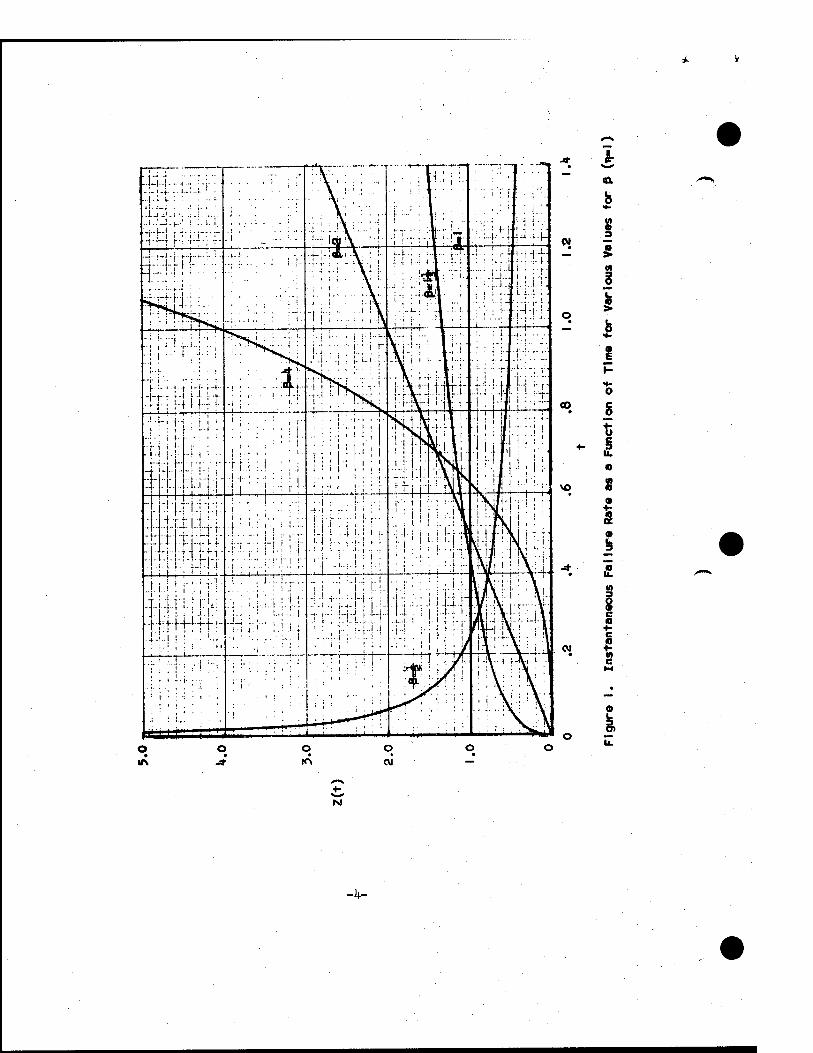
Basic factors for the design and evaluation of plans to meet
specified needs, and comprehensive tables of single-sampling plans have
been prepared and included for each of eleven values for ß, values of
t> 2> s> 1, 1 i, if, 2, 2-|, 3^-, h, and 5. This range of values covers
the range of shape parameters normally encountered with industrial and
military products. Values for ß of less than 1 apply to products
vhose distribution of failures is such that the failure rate** is high
in early life and gradually decreases vith the passage of time. This
seems to be the case for many electronic components such as transistors
and resistors. Recognition of the fact that the failure rate decreases
(or increases, for that matter) with the passage of time and allowance
for this fact is extremely important if acceptance sampling-inspection
plans for lifelength and reliability are to be applied realistically.
For ß = 1 the Weibull distribution is the same as the exponential;
the exponential distribution, in effect, being a special case of the
Weibull. At ß = 1 the failure rate is constant and does not change
with the passage of time. Use of exponential sampling plans assumes
this constancy—an assumption that may not be warranted for a large
proportion of applications. For values of ß greater than 1, the
failure rate is relatively small at the start of life or service but
increases with the passage of time, the rate of increase being larger
for larger values of ß. Thus ß-values larger than 1 may quite logically
apply for items for which wear-out or fatigue is an important cause
for failure—items such as electron tubes or many mechanical components.
As an illustration of the above comments, reference may be
made to Figure 1 which shows, for the Weibull distribution, the re-
lationship between the instantaneous failure or hazard rate (or
simply hazard), symbolized by Z (t), and life or time, t , for **See Appendix A for the definition of failure rate and its relation-
ship to hazard rate.
-3-
fr
«tx
b in
3 a >
L.
|
o
s
+- 5
c a
e
i.
N

various values for ß. The value for the location parameter, y has been
taken as zero. Also, in each case a value for the scale parameter, TJ ,
of unity has been used.
1■3 The Acceptance Procedure
The factors and the sampling-inspection plans included in this
report have been designed for use under the following acceptance pro-
cedure :
(a) Select at random a sample of n items from the submitted
lot.
(to) Place the selected items on life test for some specified
period of time, t.
(c) Determine the number of items that fail during the
period of time, t.
(d) Compare the number of items that fail with a specified
acceptance number, c.
(e) If the number of sample items that fail is equal to or
less than the acceptance number, c, accept the lot;
if the number that fail exceeds the acceptance number,
reject the lot.
Testing of sample items may be curtailed prior to time t if the
lot is to be rejected since it is possible to observe (c + l) failures
in less than t units of time.
It may be noted from this outline that the procedure is for
attribute inspection and it takes the form commonly employed for accep-
tance sampling-inspection when the lot quality of interest is simply
the proportion or number defective rather than reliability or item life.
The only variation in method is the use of a testing truncation time, t.
-5-

Under this procedure the probability of acceptance for a lot,
P(A), depends on the probability , p', of item life being less than
(or equal to) the test truncation time, t. For applications for which
the value for the shape parameter, ß, is known (or can be assumed to
approximate some known value) and for which the testing truncation
time, t, is specified, the probability p' is a function only of the
hazard rate Z(t) at time t. Since p1 is »function only of t and Z(t),
the operating characteristics for any given plan depend only on t and
Z(t). In order to provide factors and sampling tables for general use
rather than for specific values for t and Z(t), they have been provided
in terms of the product tz(t). Conversion of values for this product
to desired values when t or Z(t) is specified, will obviously be quite
easy. This will be demonstrated in the discussion of examples that
follow later.
To provide a means for the design or evaluation of sampling inspec-
tion plans, two tables of factors have been prepared. One, Table 1,
lists tZ(t) values for various values of p'. For convenience in tab-
ulation and use, p' (in $) values are used and tz(t) x 100 rather than
tz(t) values are tabulated. The second, Table 2, tabulates p1 (#)
values for various values of tz(t) x 100. In both, values are supplied
for each of the eleven selected values for ß. Through the use of these
tables, acceptance-sampling plans of any desired operating characteristics
can be designed, or specified plans can be evaluated using the math-
ematics and practices ordinarily employed in attribute inspection.
A final point of procedure that should be mentioned is that the
factors and tables of plans are for direct application in cases for
which the time t at which the hazard is specified or is to be tested is
the same as the time t at which life-testing of sample items is to
be truncated. However, a table of factors has been prepared, (Table 5;
-6-

to use in a simple modification Mii'ch allows the test truncation time
to differ from the time at which the hazard rate is specified. The
life test time for sample items can be one-half or one-fifth, for
example, of the time at which the hazard rate is specified.
-7-

SECTION 2
THE BASIC CONVERSION FACTORS
2.1 Computation of the Conversion Factors,
The instantaneous failure or hazard rate or simply hazard at any
specified time t, which may be symbolized by Z(t), may be expressed
by the relationship
Z(t) - f(t) / R (t) (1)
where f(t) is the population density function (p.d.f.) and where
R(t) = 1 - F(t), (2)
for which F(t) is the cumulative distribution function (c.d.f.)«
For the Weibull distribution (and for the case for which the value
for y, the location parameter is 0), the expression for f(t), the
population density fuction, is
f(t) = (ß/ri) (t/r,) P-1 exp t - (t/»j)P ] . (3)
Again for the Weibull distribution and for 7 = 0, the expression for
F(t), the cumulative distribution fuctlon, is
F(t) = 1 - exp [ - (t/n) ß J. (fc)
Using these expressions the hazard can now be given by dividing
Equation (3) by the unit compliment of Equation (h)f thus,
z(t) - (ß/n) (t/T)) ß_1 . (5)
-8-

For the stepe to follow, it vill be useful to multiply each side
of the above equation by (t/ß). Obis step will give täte relationship
MÜ = (t/n)ß. (6)
In the design Or evaluation of attribute sampling plans, one is
concerned with the probability of a sample item failing before the
end of the test time, t. This probability, which may be symbolized
ty P'* , is given by the cumulative distribution function (c.d.f.);
thus,
P* = P(t) = 1 -exp [ - (t/n)ß ] . (7)
Combining Equations (6) and (7), p' in terms of Z(t) becomes,
P' = 1 - exp [ - tZ(t) ] . (8)
From this expression it may be noted that upon transposing and taking
the natural logarithm that
-tZ(t) = In (1-p») or
tZ(t) « -ß In (1-p1). (9)
The two equations, Equations (8) and (9) furnish the basic
relationships for computing the factors required for the design or
evaluation of the attribute sampling-inspection pTqnp for lifelength
and reliability being considered in this study. Equation (8) may be
used for computing values for p» corresponding to given values for
tz(t) and Equation (9) may be used for computing values for'tz(t')
corresponding to given values for p*.
For convenience in computation, Equation {$) can be rewritten as,
tz(t) « ß exp ( In [-ln(l-p')] }. (io)
-9-

Values for the expression
-In [ -1» (l-p«) ] (11)
are available from a table of the inverse of the cumulative probability
function of extremes, compiled by the National Bureau of Standards.3
For both the relationship equations values for e raised to the powers
indicated were read from the National Bureau of Standards tafclae of the
exponential function.
Prom the relationship equations an important point may be noted,
which is that for the attribute form of inspection used in the acceptance-
sampling procedure, the Weibull scale parameter, ij, is not directly in vdLved
With the value for the shape parameter, ß, known or given, only the
product of test time, t, and the hazard of interest, Z(t), are of
concern. Attribute plans may he designed or evaluated in terms of
tZ(t) and with one element of this product given or assumed, the
other element may readily be determined.
In the above analysis it has been assumed that the value for r,
the Weibull location parameter, is zero. For a large proportion of
possible applications this will actually be the case. However, if in
an application y has some non-zero value, adaptation of the procedure
to allow for this is quite easy. All that must be done is to subtract
the value for y from the value used for t to get a converted value ,
t~ Ihis converted value is then applied to form a converted product
tQZ(t0) which can be used for all computations and readings from the
table. Any solution in terms of tQ can then be converted back to real
values by simply adding the value for y.
2.2 The Tables of t'aatqrs and Their Use.
With the use of Equation (9) a table of vaiuey for tz,(t) for
various values of p* has been prepared. It is presented at the end of -10-

. %
this report as Table 1. For convenience in tabulation and use, p'
values have been multiplied by 100 and expressed as percentages and
values for tz(t) have likewise been multiplied by 100 to give tz(t)
x 100 values, The values used for p' range from .010$ to 80# with the
selection made in accordance with a standard preferred number series.
Also, through the use of Equation (8), a table of values for p' (<f>)
for various values for tz(t) x 100 has been prepared. It will be
found presented as Table 2. With this table, values for p' {$) may
be found without interpolation when rounded values for tz(t) x 100
are given. The two tables provide the basic factors necessary for the
design ex evaluation of attribute sampling Jaspeetion plans of the form
described in the previous section of this report. Two examples of their
use follow.
Example (l)
One possibility of use for the conversion factors is in the
evaluation of specified acceptance sampling plans. Suppose, to consider
a simple example, a single-sampling attribute plan has been specified
with a sample size, n, of 115 items and an acceptance number c, of 3
items. The test time for the sample items is to be 500 hours. A value
for ß of 2 and a value for 7 of 0 seem reasonable to assume. The
operating characteristics for the plan under these conditions must be
determined. Lot quality is to be evaluated in terms of the hazard at
500 hours of use.
Under plans of the form presented here,the probability of accep-
tance for a lot, P(A), depends on the probability, p', of an item
failing before the end of time, t, nhich in this case is 500 hours.
The first step, then, in determining the operating characteristics
is to determine the probability of acceptance, P(A) associated with
each of an appropriate range of values for p'. These probabilities
-11-
may be determined by one of the methods commonly used in the evaluation
of ordinary attribute sampling inspection plans. It is most convcniert
to make use of the readily available tables of the hypergeometric dis-
tribution, of the binomial distribution, or of the Poisson distribution—
the choice depending on the ratio of the sample size to the lot size,
the size of the sample,the range of p' values involved, and on the
accuracy desired. If the plan happens to be one matching an existing
attributes plan of the ordinary form (for defectives) for -which ah oper-
ating characteristic curve has been prepared, the required values for
the probability of acceptance may be read from this curve to sufficient
accuracy for ordinary use. For the example under discussion, the
values for P(A) corresponding to each of a suitable series of p' values
are listed in the tabulation below (in the second and first columns,
respectively). Note that the p' values have been selected from those
used in the construction of the table of conversion factors (Table 1)
and that the range of p' values used is the range required to give
values for P(A) for most of the range from 1.00 to 0 so that a complete
picture of operating characteristics may be obtained.
One next step is to make use of the first of the tables of con-
version factors, Table 1, and read off the value for tz(t) x 100
corresponding to each of the listed p' (in $) values. These are found
in the seventh column of factors in Table 1, the column for ß = 2.
The values for this example are listed in the third column of the tabula-
tion below.
The final step is to divide each of the values tabulated for tz(t)
by the value specified for t, which is 500 hours, to give the associated
hazard, Z(t). These computations have been made with the results as
listed in the last column of the tabulation below.
-12-

It may now be noted by scanning the figures in this last ■column
that for a lot made up of product whose hazard is 4.83 x 10"^ at 500
hours, the probability of acceptance will be -95; if, on the other
hand, the hazard is 26.88 x 10"5, the probability of its acceptance
is only .06, for example . If desirable, each P(A) value and its
associated z(t) value may be plotted to construct an operating char-
acteristic curve. This has been done for this application with the
resulting curve being the one shown for ß = 2 in Figure 2. To provide
some indication of the sensitivity of the acceptance-inspection pro-
cedure to changes in the value for ß, the shape parameter, operating
characteristic curves have been prepared and presented in Figure 2
using the same plan and the same value for t, but with other values
for ß, values of 1 and 4 with the value 1 representing the exponential
distribution commonly assumed in reliability work.
p' (in <f>) P(A) tZ(t) x 100 Z(t)
• 5 •99 1.002 2.00 x 10"5
,8 .98 I.606 3.21 x 10"5
1.0 •97 2.010 4.02 x 10"5
1.2 • 95 2.4l4 4.83 x 10"5
1-5 .90 3.O22 6.04 x 10"5
2.0 .80 4.040 8.08 x 10"5
2.5 ,68 5.064 10.13 x 10"5
3-0 • 55 6.092 12.18 x 10"5
4.0 •33 8.164 16.33 x 10"5
5-0 •17 10.258 20.52 x 10"5
6.5 .06 13.442 26.88 x 10"5
8.0 .02 16.676 33-35 x 10"5
n = 115 c = 3 t = 500
-13-

IA
'o 6 t-
IA
'o
i IA
A IA
1 UN o "*
ft C
b >*■
IA $
3 u
t £ M • «M>
us a b i a. t; * 8
M 1 u a» c
IA +• 1 a o b i s
ei a
IA k 'o 8» <s ' u.
8 R S £ S R 3 R S 2 S • ••• ••••
(V)d - eoue+deODV +o A+||jqoqoJd
- O
■|1>~

In connection with this example it may be well to note that any
double-sampling or multiple-sampling plan that "matches" the single-
sampling plan in ordinary attributes sampling—that is, for which the
same P(A) values are associated with each value for p'—will provide
the same operating characteristics in terms of hazard, z(t). For
the plan used in this illustration, for example, a matching
double-sampling plan is one for which the first sample size is 75 and
and the second 150, with an acceptance number of 1 and a rejection
number of 6 for the first sample and an acceptance number of 5 and a
rejection number of 6 for the combined samples. One only changes in
procedure required will be those normally associated with multiple
sampling plans. 3he value for t specified for single sampling will be
used for both the first and the second sample. Double-sampling and
multiple-sampling offer excellent opportunities for reducing, over the
long run, the average amount of acceptance inspection. However, in
testing for life and reliability the added elapsed time required for
testing when a second or subsequent sample is required may be a serious
obstacle to application of this form of sampling.
Example (2)
Another possibility for use of the basic factors is in the design
of an acceptance sampling plan to meet specified requirements. Consider
the case of a manufacturer who is to purchase in large quantities a
certain electronic component. Experience in the testing and use of
this component has indicated the Weibull distribution applies well as
a statistical model with a value for ß, the shape parameter, of 1 1/3
and for y , the location parameter,of 400 hours. A test period for
sample items of 1200 hours has been agreed upon. Experience with the
product has further indicated that a competent supplier should be able
to submit lots for which the hazard at 1200 hours is .000044 (per hour).
-15-

Accordingly this value for z(t) is to be adopted as the Acceptable
Hazard Rate (AHR) and a plan is desired for which acceptance is virtually
certain, say with P(A) = .99, if a lot is this good or better. That
is>P(A | AHR) fe .99 where AHR = .OOOOMf at 1200 hours. Furthermore,
the user has ascertained that if the hazard for a lot or shipment
is .000155 (per hour) or more, use of the components will lead to
much difficulty. Thus a low probability of acceptance, sey .05 or
less, is desired. Accordingly the Rejectable Hazard Rate (RHR) is
.000155 at t » 1200 and a P(A|RHR) S .05 is specified.
The first step in the design of the plan is to subtract the value
for 7 , the location parameter, from the time t to give a new time,
tQ, in terms of 7 = 0. Accordingly, tQ = t - y or tQ = 1200 -
1*00 = 800 hours. The next step is to compute the tQZ(t0) x 100
product at both the Acceptable Hazard Rate and the Rejectable Hazard
Rate, using the value determined for tQ. Obese are:
t0Z(tQ) x 100 = 800x.OCO0W x 100 = 3-52 (at the AHR),
t0Z(tQ) x 100 = 800 x .000155 x 100 = 12.\ (at the RHR).
(12)
With the use of Table 2 these computed values can now be applied
to determine the probability, p' , of an item failing before the end
of 1200 hours (tQ = 800) under both the above conditions. These
values (for ß = 1 l/3) may be read, through linear interpolation, as:
p' = 2.605 $ or roughly, 2.6# (at the AHR),
p' - 8.87 $ or roughly, 8.9# (at the RHR) (13)
Finally, a sampling plan may be determined, using procedures
commonly employed to design sampling plans of the usual form for
attribute inspection. For this case a plan is required for which
-16-

P(A) * .99 when p' = 2.6<f> and for which P(A) £ .05 when p' = 8.9$.
Making uee of factors prepared by Cameron'' (which are based on the
Poisson distribution) it will be found that an acceptance number, c,
of 10 will provide most closely the required characteristics and that
a sample size of 184 will give a P(A) = .99 if P* = 2.6#. A check
using other factors supplied at the same source indicates P(A) = .05
if p' = 9.2$. Similar reeults for n and c may be obtained by using
the beta probability ohart (which is based on the binomial distribution)
_, ,. ■ 6 given by Kao . Ihus this 1
closely the specifications.
given by Kao . Ihus this plan, n = 184, c = 10, t = 1200, meets
-17-

SECTION 3
THE TABLES OF SAMPLING PLANS
3.1 Construction and Use of the Basic Tables.
An extensive collection of sampling plans has been desisned,
with a separate table prepared for each of the eleven representative
values for ß for which the relationship between tz(t) and p' has been
determined. These tables of plans will be found at the end of this
report as Tables 3a through 3k.
Each table lists 208 single-sampling plans, with the acceptance
number, c, and the corresponding sample size, n, given for each. The
plans have been cataloged in terms of a Rejectable Hazard Rate (RHR)
under the assumption that for components for which the quality of
interest is reliability or lifelength, consumer protection will be of
most conero. The figure in each column heading is the tz(t) x 100
product for which the probability of acceptance under the sampling
plans in that column is .10 or less. Expressed otherwise, the column
headings are percent values of t i RHR, and for the plans below each
the P(A | RHR) S .10.
However, the tables also provide guidance for selection and
evaluation of plans in terms of the Acceptable Hazard Rate, (AHR).
-18-

^e figure in parentheses below the sample size number, n, tor each
Pia, i. the per cent value of t x AHB product for which the prob-
ability of acceptance is .95 or mre. Wlth ^ w Qf ^ ^^
a plan can be selected in terms of an Acceptable Hazard Rate, if one
so desire,, m any case the two tZ(t) x 100 products broadly describe
the operate characteristics of the plan wi* which they are associated
^ay thus provide a basis for the appropriate choice of a plan, or
for determining the operating characteristics of a plan that has been
specified or is being applied. Illustrative examples of the use of
the tables of plans will be found below, when tZ(t) x 100 table values
to match computed or given values cannot be found, linear interpolation
between table values that are available will give solutions that are
precise enough for most practical purposes.
Ibese plans have been designed under the assumption that the
size of the sample will be relatively small compared to the size of
the lot (an assumption imposed under almost all other published sets
of plans). Under this assumption the number of failures prior to
time t approximates the binomial distribution.. Binomial tables com-
piled by GW were used to prepare some of the plans, those for
values for c from o to 9 «d for values for n up to 150. Por values for
c from 10 to 15 and for n up to 60 or so, Pearson's tables of
Plete-beta function8 were used. Plans rearing higher values for n
were determined by using the Poisson approximation, making use of tables "
Prepared by Cameron.* At each point Qf ^ ^ ^ ^^ ^ ^
Poisson the match in values for n was checked and found to be close. ffie
slight differences, usually 1 or 2 items, that were found were on the
conservative side, the value for the sample size being slightly larger
than the size theoretically required.
-19-

Example (3)
A receiving inspection plan is recuired for a certain product.
Experience has indicated a value for ß of 2/3 can be assumed and a
value for y of 0. It has been determined that lots with a hazard rate
of .00005 (per hour) at 1000 hours of use for the product will be
considered an unsatisfactory rate and - can be used as an RHR value.
The test time for sample items will be 1000 hours, the same value for
t used in specifying the EHR. Testing facilities are available to
test as many as 200 items at one time.
Computation of the tz(t) x 100 product at the RHR gives 1000 x
.00005 x 100 or 5.0. Plans for this value must now be found in Table
3c, the table of plans for ß = 2/3. Any plan under the column headed by the
value 5 will give a probability of acceptance of not more than .10 at the
RHR value of .00005. If full use is to be made of the testing
facilities, the plan with an acceptance number, c, of 9 and a sample
size, n, of 197 may be employed. With this plan, the 'tz(t) x 100
product for a P(A) = .95 is 1.8. Simple substitution in the product
gives 1000 x Z(t) x 100 = 1.8 from which it will be found that Z(t) =
.000018. If the producer submits product with this hazard rate or
less (at 1000 hours), his risk is low; the probability of acceptance
will be high, namely .95 or more.
Example jk)
Consider another application for which a plan is to be selected.
In this case, ß = 1 l/3 and 7 = 1250 hours. A Rejectable Hazard Rate
of .000020 and an Acceptable Hazard Rate of .000008, both measured at
2000 hours seem to be most suitable. The test time, t, is also to be
2000 hours.
-20-

Since ß = 1 1/3 can be assumed, a plan from Table 3« can "be used.
First, a new time, tQ, in terms of y = 0 must be found. From t0 *
t - y or tQ " 2000 - 1250, a value for tQ of 750 hours is found. Ne::t,
the tQz(to)xl00 products at the AHR and the RHR can be confuted, using
tQ or 750 hours. They are:
750 x .000020 x 100 - 1.5 (at RHR)
750 x .000008 x 100 = .6. (at AHR) (l^)
Any plan in Table 3e under the column headed by the product 1.5 will
meet the EHR requirement. Scanning this column in terms of the products
in parentheses, the plan using an acceptance number, c, of 10 and a
sample size, n, of I38O is selected. For this plan, the P(A|RHR) = .10
and the P(A|AHR) = .95, the probabilities of acceptance being these
figures at the designated hazard rates and at a life of 2000 hours.
3.2 The Dependence of Operating Characteristics on Sample Size
An interesting and somewhat useful characteristic of the form of
plans presented in this report is that the ability of a plan to dis-
criminate between good and bad lots depends on the size of the acceptance
number rather than on the size of the sample; operating characteristic
curves become steeper as the magnitude of the acceptance number is
increased rather than becoming steeper as the size of the sample is
increased as under the usual forms of sampling inspection. For given
magnitudes for consumer and for producer risks at the Rejectable Hazard
Rate and the Acceptable Hazard Rate respectively, a nearly constant
ratio between the Rejectable Hazard Rate and the Acceptable Hazard Rate
will be found for any given value for the acceptance number. For the
collection of plans presented here,the ratio is constant (for all
practical purposes) for all plans for which the tZ(t) x 100 value
-21-

et the RHR is more than 5- For values less than 5, there is a slight
decrease in the magnitude of the ratio as sample sizes become increas-
ingly small, but not enough to be significant for practical purposes.
Not only is the ratio between the Rejectable Hazard Rate and the
Acceptable Hazard Rate constant for any given value for c, but any
ratio computed for any given pair of consumer and producer risks
applies for all values for ß; the ratio does not depend on ß as is
the case for the Weibull sampling plans that test lots in terms of
mean Item life.
A table of hazard rate ratios for values of c from 0 to 15 has
been prepared for a number of alternatives for consumer risk and
producer risk values. They are presented as Table h. As indicated,
the figures in the body of the table are approximate values for RHR/
AHR for each value for c for the acceptance probabilities indicated
in the table headings. The use of this table will be described by
giving two examples.
Example (5)
Consider the case described in Example 2 in which the desired
sampling plan was to give a probability of acceptance of .05 cr less if the
hazard rate was .000155 and a probability of acceptance of .99 or mere if the
hazard rate was.OOOOM*, That is the P(A | RHR) s .05 and P(A | AHR)g
.99« In using this table (Table h) one first determines the value for
the ratio RHR/AHR which is .000155/.OOOOW or 3.52. Next, the table
is scanned in the column giving ratios for P(A | RHR) = .05 and
P(A I AHR) = .99* looking for a value close to tue computed ratio. A
value close to it, 3.56, is found opposite c = 10. Thus an acceptance
number of 10 will be required. This, it will be noted, is the
acceptance number that was determined in other ways in the previous
-22-
^"*s

example. Table h provides a quick, short-cut way of finding c, the
acceptance number for any application (within the limits of the table).
Example (6).
A plan is required for a product for which ß = 3 1/3 and 7 = 0,
for which a Rentable Hazard Rate of .0005 per hour has been estab-
lished, and for which a P(A | RHR) s .10 will be satisfactory. The
test time, t, is to be 50 hours. Furthermore, a high probability of
acceptance, .99, is required at the Acceptable Hazard Rate, which has
been established as .0001 per hour.
The tZ(t) x 100 product at the RHR is 50 x .0005 x 100 or 2.5.
Referring to .Table 3i vhich contains plans for ß = 3^ any plan in
the column with the 2.5 value heading will give the RHR risk of s .10
specified. The one to select can be determined by use of Table k.
The RHR/AHR ratio for this case is .0005/.0001 or 5. At a P(A | AHR)
£ .10 and a P(A | AHR) & .99, Table k indicates an acceptance number,
c, of 5 will give most closely the operating characteristics desired.
The RHR/AHR ratio has a value of 5-20 which is close to the value of
5 obtained for the specified rates. Thus the plan to use is the sixth
one down in the column (headed 2.5) in Table 3±, the plan for which
c = 5 and n = 12^0.
3-3 Differences in Lifetesting Time
In order to prepare tables of factors and sampling plans for
general use, it has been necessary to assume that the lifetesting
time for sample items will be.the same as the time, t, at which hazard
rates are specified or are to be determined. However, a simple modifi-
cation of the procedure can be made to allow for cases in which the
-23-

two times do differ. All that must be done is to determine the hazard
rate at the test truncation tune which corresponds (for the value for
ß that applies) to the hazard rate at the specification time.
A table of hazard rate ratios, Table 5> has been prepared for
making this conversion. The table gives for various values of t„/t,
values for the ratio Z(t„) / Z(t.) for all the ß-values concerned ...*■'■
in this study. Also, a chart has been prepared, Figure 3> showing
the relationship between hazard rate and time for the same values for
ß. Die two may be used interchangeably, the chart being useful for
cases in which table values are not available and the table being
useful when more precision is required and one of the tabulated table
values applies to the case at hand. If Z(t.) represents a specified
hazard rate and t2 the time at which it is specified, then z(t,) can
be used to represent the corresponding hazard rate at some other time,
t,. 3he table can also be used for cases in which the test-truncation
time is greater than the time at which the hazard rate is specified
(if such cases are encountered). All that need be done in such cases
is to reverse the meanings given to the subscripts 1 and 2. Conversion
from one hazard rate to another or from one time to another when
necessary to make use of the factors and plans presented here is quite
easy, as vill be shown in the example which follows.
Example (7)
A plan is required for a case for which a hazard rate specified
as an RHR (at a P(A) = .10) is .000375 at lj-000 hours. However, a test
truncation time of 1000 hours must be used. A sampling plan in terms
of the specification but using the shorter testing time is required.
A value for ß of 1 2/3 and for y of 0 can be assumed.
-24-

*(% **;>
i: t-i-rt-iit.
? 6 7 8 9 io ' ' T2/
Figure 3. Die Belatlonship Between Hazard Bate and W»e for Various Values torß
-25-

The value for t2/t in this case is ItfXDO/lOOO = k. Reference to
Table 5 indicates for this tg/^ ratio and for ß = 1 2/3, that the
Z(tg) / Z(tx) ratio is 2.52. Substitution of .000375 (the RHR) for
Z(t2) gives .000375 / Z(tx) = 2.52 or Z^) = .00015- This equivalent
value, Z(t,), of .00015 »ay BCV be used to select a plan to use with
the 1000 hour testing time. «Hie product tz(t) x 100 to apply is thus
1000 x .00015 x 100 * 15. A plan may now he selected from those given
in Table 3f f or ß = 1 2/3. Any plan under the column with a heading
value of 15 will meet the RHR requirement. Suppose testing facilities
are available for as many as 150 sample items and so the plan for which
c = 8 and n = 1^9 is to be applied. A reversal of the above pro-
cedure can be used to make use of the tZ(t) x 100 product given (in
parentheses) for this plan in Table 3f for a P(A) £ .95 to determine
the Acceptable Hazard Rate. The product tz(t) x 100 is 5 J*. At the
shortened testing time of 1000 hours, 1000 z(t) x 100 = 5-^ or Z(t) =
.00005^. For lots with this hazard rate at 1000 hours, the P(A) § .95-
The corresponding hazard rate at UOOO hours can be found from the
hazard ratio obtained from Table 5. Since Z(tg) / Z^) = 2.52,
Z(t2) / .00005^ = 2.52 or Z(t2) = .000136. Lots with this hazard
rate at 1*000 hours have a probability of .95 or greater of acceptance;
the rate can be used as the Acceptable Hazard Rate at this specified
time.
-26-

SECTION k
AVERAGE HAZARD PLANS
The average hazard over any specified time period up to t,
which is denoted by m(t)> may be expressed as,
»<*> "k I» Z(y)dy = M(t) 1 t (15)
where Z is the hazard function defined by Equation (l) and M(t) is
called the cumulative hazard over t. For a lifelength distribution
which starts at time y (the threshold or location parameter), the
lower limit of the integral M(t) should be 7 which is assumed to be
zero in this report.
Following from Equation (Al4) of Appendix A, the probability of
a sample item failing before the end of the test time t is then,
p' = F(t) = 1-exp [- tm(t) ], t>0. (l6)
From this, it may be noted that
tm(t) = - In (l-p')> 0 <p' < 1. (17)
These two equations form the basic relationship for the design
or evaluation of the attribute sampling-inspection plans using the
average hazard, m(t) as a life quality criterion. By direct comparison
of these two equations with Equations (8) and (9), it may be noted that
m(t) plays the role of z(t) with ß = 1. For this reason, no additonal
tables need be prepared for sampling plans where the average hazard,
m(t) is specified. Furthermore, since Equations (l6) and (17) are valid
for any arbitrary distribution, the sampling plan based upon the average
-27-

hazard is non-parametric,1 i.e., distribution-free.
Nevertheless it is useful to equate Equation (l6) with the ex-
ponential c.d.f., F(t) = 1-e*'0 = l-e"U , for t, 9 , X > 0, ana to
note that m(t) = X. Writing this conversely by letting m" be the
inverse function of m,
t = m"1 (X) = T. (18)
where T is called the hazard-breakeven time. For any lifelength
distribution with a monotonically decreasing (or increasing) failure
rate or hazard rate in time, the T^ , the hazard-breakeven time represents
the point in time when the average hazard of the lifelength distribution
under consideration is equal to the specified constant hazard (for the
exponential case). But when the monotonicity assumption is removed,
then there may be multiple solutions for Equation (l8), depending upon
the nature of m(t).
For maintainable equipment, in contrast to the so-called one-shot
equipment such as a fired missile, the average hazard for the component
therein represents the average amount of replacement necessary to keep
the equipment In operation. Hence it is significant to consider the
hazard-breakeven time. If X is the tolerable average hazard, then for
a component with a monotonically decreasing failure rate, T^ means the
equipment break-in time, while for a component with monotonically in-
creasing failure rate, T. means equipment retirement time. Two numerical
examples will follow.
Example (8)
Suppose the lifelength distribution is of the Weibull form.given
by Equations (3) and (h), then Equation (17) becomes,
tm(t) = (t/fl)P (19)
-28-

and Equation (l8) becomes,
TX= [xa ] ^P"1) (20)
where a = v, is the Quasi-scale parameter of the Weibull distribution2
Consider the case of a manufacturer who is producing a certain
electronic component. Experience has indicated that a Weibull dis-
tribution with y » o, ß * 1/3, and T) = te.875 x 10 9(or a = 3,500)
applies. A customer specifies a value for X = 6$ per thousand
hours. The hazard-breakeven time T^ in this case is computed as
follows. The per hourvalue for X. is, X = 0.06/ 1D00 ^ 5 x lO"-5
(per hour). Substituting this into Equation (20) gives,
\ = (3,500 x 6 x 10"5) -<3/2). = 10#39 hours#
That is, if the equipment in which the component is to be installed
is allowed to break-in for a period of approximately ten hours, then
thereafter the average hazard of the component will be less than that
specified by the customer—a very comforting assurance.
Example (9)
Suppose the manufacturer in Example (8) has decided to truncate
the lifetest at 1000 hours and desires a sampling plan which will
accept with high probability (say .98), lots having an average hazard
of 0.6$ / 1000-hrs. and reject with high probability (say .90),
lots having an average hazard of one order of magnitude higher (i.e.,
6fJ 1000-hrs.). in this case, the producers risk is 2# and the
consumer's risk is 10# which gives a 9056 confidence coefficient of
shipping products with 6% / 1000-hrs. or better average hazard.
-29-

The values for -tm(t) :c 100 are 0.6 and 6.0 at P(A) = .98 and
P(A) = .10 respectively. By linear interpolation in Table 2 for ß = 1,
the following values for p' are found:
At P(A) = .98, p" = .00597 or approx. 0.6$
At P(A) = .10, p' = ,05821 or approx. 5.856 (21)
The sample size, n, and the acceptance number, c, of the desired sampling
plan may be determined from the requirements specified by Equation (21).
The use of the beta probability chart gives c + l = 3,n-c = 90,
or n =92 and c = 2.
-30-

SECTION 5
ADAPTATION OF THE MIL-STD-105C PLANS
5.1 Use of the MIL-STD-105C Plans for Life and Reliability Testing
in some cases it may be advantageous to employ the familar Military
Standard 105-c plans for reliability and lifetestlng applications. To
make this possible, the basic conversion factors described in Section 2
have been employed to find tz(t) x 100 products for all the plans in
the MIL-STD-105C collection. Just as for the basic tables of plans
described in Section 3, separate tables of products have been prepared
for each of a number of selected values for ß, the Weibull shape
parameter. The special case for ß = 1, which is the exponential case,
has been included.
The acceptance procedure to be used is the same as that employed
for the basic plans and as outlined in Section 1.3. For single sampling
the steps are (a) select a suitable sampling inspection plan, making use
of the tables of products provided, (b) draw at random a sample of n items,
as specified by the plan, (c) place the sample items on life test for
the specified period of time, t, (d) determine the number of sample items
that fail during the test period, (e) compare the number Of items that
fail with the acceptance number, c, specified for the plan, and (f) if
the number that fail is equal to or less than the acceptance number,
accept the lot; if the number failing exceeds the acceptance number,
reject the lot.
Both the sample sizes and the acceptance numbers used vilj, be
those specified for the MIL-STD-105C plans. For convenience, the single-
-31-

sample sizes and the corresponding acceptance numbers have been included
in this report and will be found in Table 7. Single sampling will
presumably be usdd, but by simple modification double sampling or
multiple sampling can be used if desired. It may be noted that the
acceptance procedure for any form of sampling is the same as that
specified for the MIL-STD-105.C plans with the single exception of the
use of a test truncation time, t.
The eelection of a suitable plan, the determination of operating
characteristics in terms of hazard rate for a specified plan, and the
determination of an appropriate life-testing time are all made through
use of the tables of products which will be found at the end of this
report. Ways for making use of these tables will be discussed in the
section that follows and in the accompanying illustrative examples.
It may be noted that the probability of acceptance for a lot under
the procedure outlined above depends only on the probability, which may
be designated by p', of an item failing before the end of the test period,
t. The actual life at which an item fails need not be determined; inspec-
tion is on a attribute basis. For this reason it is possible to use the
105B plans to evaluate submitted lots in terms of hazard rate, Z(t), at
some specified time, t. The operating characteristics for any sampling
plan specified by c and n depend only on t and Z(t). A brief outline of
the mathematics involved in the procedure will be found in Section 2.1.
To provide a procedure of simple form and one suitable for general
use, the tables of factors for adapting the 105C plans to use in terms of
hazard rates have been prepared in terms of dimensionless products of
t times Z(t). Actually, in order to give figures that may be more
-32-
conveniently used, the tables are composed of tz(t) x 100 products. Each
of the I05C plans Is cataloged in terms of such tz(t) x 100 products.
These product values are to he used in much the same way that percent
defective values are used in the selection and application of plans for
ordinary attribute inspection. With t and Z(t) specified, all that must
be done is to compute their product and then select a plan in its terms.
If on the other hand, a plan (n and c) and a test truncation time (t)
are specified, the product may be used to give an evaluation of operating
characteristics in terms of hazard rate, Z(t). Or, alternatively, the
product may be used to find a suitable test truncation time, t. Examples
of such application of the factors will be found in the latter part of
this section.
The Weibull distribution, one will recall, is a three-parameter
distribution, requiring a location or threshold parameter, a scale
parameter, and a shape parameter for complete description. For the
procedure and plans presented here, the scale parameter need not be
ascertained or known; the tz(t) x 100 product contains information on its
magnitude. For the location or threshold parameter (commonly symbolized
by the letter 7), a value of zero is to be assumed in the direct appli-
cation of the products and the procedure. For many applications a 7
value of 0 will apply; there will be no initial period of life free of
risk of failure. This assumption is equivalent to knowing the value for
gamma. If 7 has some non-zero value, all thit is necessary is to subtract
the value for 7 from t to obtain a value tQ and then use tQ rather the»
t in working with the tables of products. The third parameter, the
Weibull shape parameter (which is commonly symbolized by the letter ß)
'-38-.

must be known. Hie products depend on the value for ß so that its
magnitude must he known or estimated from past research, engineering,
or inspection data. Separate tables of products have been provided for
each of eleven values for ß, values ranging from 1/3 to 5. The assumed
value for 0=1 represents the special case of the exponential distribution
and so may be used when this distribution seems to be the most appropriate
statistical model. Estimation procedures for ß or 7 are available and
may be found in the papers by Kao ,'2'' '22'.
One final point of procedure must be mentioned. It is that for the
direct use of the tables of products, the item life at which the hazard
rate is measured or specified and the life at which the testing of
sample items is truncated are assumed to be the same. That is, the t
used in the tZ(t) x 100 products is the same as the test truncation.time,
t. Howevery if the life at which hazard rates are to be specified or
evaluated must differ from the test truncation time, a simple variation
in procedure may be made to allow for any desired departure. All that.
must be done is to find (for the value for ß assumed) the hazard rate
at the test truncation time that corresponds to the hazard rate at the
time used in the specification or at which lots are to be evaluated. A
table of hazard rate ratios has been compiled for this purpose. It
will be found as Table 5 at the end of this report. The method for its
use will be described in one of the illustrative examples which will
follow.
g.g The Tables of Products and Their Use
To provide the necessary data for using the 105C plans in life and
reliability testing in terms of hazard rate, eleven tables of tz(t) x 100
products have been prepared. One is available for each of the following
values for ß: f *,f, 1, i*, if, 2, 2*, $, k, and 5- These values
-34-

encompa68 the range of shape parameter values that will commonly be
encountered. For values of interest for which no table has been provided
(but within the above range), linear interpolation will give factors
accurate enough for most practical purposes. The tables of factors have
been included at the end of this report as Tables 6a through 6k.
Each table provides tz(t) x 100 products for each 1Q5C plan, that is
for each combination of Sample Size Code Letter and Acceptable Quality
Level the IO5C Standard utilizes. The factors apply not only to the
single-sampling plans, but also to the matched double-sampling and
multiple-sampling plans. The sample sizes corresponding to each Sample
Size Code Letter and the acceptance and rejection numbers applying to
each Acceptable Quality Level as found in the 105C Standard are thus
to be used in the procedure presented in this paper.
Across the top of each table will be found tz(t) x 100 products
corresponding to each of the Acceptable Quality Level values utilized ir.
the 105C $ables. Each of these matched tz(t) x 100 products provides
for all of the 105C plans of the corresponding Acceptable Quality Level
a measure of lot quality for which the probability of acceptance is
high. The producer's risk will be low with its actual magnitude being the
same as that experienced under normal use of the 105.C plans. It will
be recalled that this risk varies, being as low as .01 for large sample
sizes and as high as .20 for small sample sizes. The risk associated
with a specific plan may be obtained from the operating characteristic
curves provided in the 105C standard.
Within the body of each table will be found tz(t) x 100 products for
each plan for which the probability of acceptance is low. In each case
-35-

this probability is .10 or lese. Biese products may be used as a means of
estimating the consumer's risk when a Rejectable Hazard Rate is to be
determined or when a plan is to be selected in such terms. Thus with
pairs of factors provided for use in terms of both an Acceptable Hazard
Rate as found across the top of each table and a Rejectable Hazard Rate
as found within the body of each table, plans may be selected or evaluated
in terms of either the producer's risk or the consumer's risk or both.
Recently a revision"C" of MIL-STD-105 included., among other
things, the listing of LTPD values as consumer's protection measures as
well as the AQL values. *23'
The interpretation of these tz(t) x 100 products may be demonstrated
by means of a simple example. Suppose that for a product to be submitted
to acceptance inspection ß can be assumed to have the value of % and 7
a value of 0. Life testing of sample items is to be truncated at 500 hours.
A single-sampling plan for Sample Size Code Letter H and an AQL of 1.5$
has been specified for use (n, the sample, size will thus be 35 and c,
the acceptance number, 1). Reference to Table 6b which contains
products for ß = l/2 shows that the tz(t) x 100 product at the Acceptable
Quality Level of l.yf, is .756. With t = 500 thus 500Z(t) x 100 = .756.
Z(t), the hazard rate, can thus be computed as z(t) = .756^00 x lOO) =
.OOOOI51 (per hour). Accordingly, this figure, .OOOOI51, can be
considered as the Acceptable Hazard Rate (as measured at 500 hours of Life).
Next, by entering the body of the table at Sample Size Code Letter H
and an AQL of 1.5$, the tZ(t) x 100 product for which the probability of
acceptance is low (.10) is 5.5. Again with t = 500, 500Z(t) x 100 =5.5
or Z(t) = 5-5/(500 x 100)= .00011. Thus the Rejectable Hazard Rate (at
500 hours of life) is .00011 (per hour). These two figures found for
Z(t) may be interpreted thus, (a) lots for which the hazard rate for
-36-

items at 500 hour6 of life is .0000151 per hour or lees will have a
high probability of acceptance (examination of the 0C curves in the
105C.Standard indicates the probability is slightly more than .90);
lots for which the hazard rate for items at 500 hours of life is .00011
will have a low probability of acceptance (namely .10 or less).
Example (lO):
A purchased electronic component is to be inspected, lot by lot, for
lifelength by sampling inspection. The MIL-STM.05C plans are to be
employed. The lot quality of interest is the hazard rate at a life of
500 hours. From past experience with the component it has been determined
that the Weibull distribution can be applied as a statistical model and
that a value for ß, the shape parameter, of 2/3 can be assumed and a
value for 7, the location or threshold Parameter, of 0 can be expected.
Normal inspection is to be employed and the lot size in each case will
be 3,000 items. A plan employing an Acceptable Quality Level (in terms
of the percent defective as used in the standard) cji 4.0$ and a test
period of 500 hours have been tentatively selected, with single sampling
to be utilized Under these given conditions, the acceptance procedure
and the operating characteristics in terms of hazard rate at 500 hours
are to be determined.
By referring to Table III of MIL-STD-105C it will be found that for
Inspection Level II (which is customarily employed unless there aye
special reasons for doing otherwise) and for a lot size of 3",000,
Sample Size Code Letter L should be employed. Next, reference to Table
TV-A of the same Military Standard or to Table 7 of this report shows
-37-

that for Sample Size Code Letter L the sample! size for single sampling
is 150 items. Further reference to this lati :r Table shows that for the
4.0$ Acceptable Quality Level selected the acceptance number to use
is 11 and the rejection number 12. The acceptance-rejection procedure
will accordingly be; 7
(a) Draw at random from the lot a samp'.e of 150 items.
(b) Place the sample items on life te;r, for 500 hours.
(c) Determine the number of sample itifas that fail prior' to the end of this test period. J' . " .
(d) If the number that fail is 11 or less, accept the lot; if the number that fail is 12 or more, ra.ject it.
The operating characteristics of the m>ove acceptance procedure in
terms of hazard rate can be determined by reference to Table 6c which
will be found at the end of this report, 'fya table lists tz(t) x 100
products for application when P = f. Examination of the factors across
the top of the table (immediately below the |AQL figures in p'(#)) ♦«Shows i
that at k.0<f> the corresponding tz(t) x 100 dotio is 2.72. With t = 500
and with tz(t) x 100 = 2.72, the hazard ratej is thus determined by:
500Z(t) x 100 = 2.72
z(t) = —Si3S = .00005H . 500 x 100
This figure may be considered as an Acceptable Hazard Rate (AHR). Thus
if the quality of the submitted lot is such that the hazard rate at 500
hours is .000054V(per hour), the probability of its acceptance will be
high.* By reference to Table VI-L of the Military standard, operating
characteristic curves for single sampling for Code letter L may be
found. The curve for a 4.0$ AOX indicates that at 4.0$ the probability
-38-

V/-
of acceptance is slightly more thun .$Q, the producer's risk, then for lots
for which the hazard rate is .00005^ at 500 hours is I.OO-.98 or .02.
A Rejectable Hasard Rate (RHR), a rate at which the probability of
acceptance wil3. be low under the above plan, may also be determined by
further reference to Table 6c of this report. In the body of this table
at Sample Size Code Letter L and an AQJL of 4.056, a second tz(t) x 100
product for the application, one whose value is 7.9, will be found. This
is the product for which the probability of acceptance is .10 or less.
Using t = 500 and making another simple computation gives:
500Z(t) x 100 = 7.9
Z,(t) = 1^ = .00016 500 x 100
This answer may be considered as a Rejectable Hazard Rate (RHR). If the
lot quality is such that the hazard rate is .00016 (per hour) at 500 hours
of life, the probability of acceptance for the let will be low, namely
.10 or less. This figure quantifies the consumer's risk at the
Rejectable Hazard Rate of ,00016.
Example (ll):
For another illustration of use, consider a sampling inspection
application for which an Acceptable Hazard Rate of .000025 (per hour)
and a Rejectable Hazard Rate of .00015 (per hour) with both at" 1000.-hours
of life is required. A value for ß of if and for 7 of 0 can be
assumed. The test time for sample items is to be 1,000 hours with double
sampling to be employed. The problem is to select from the MIL-STD-105C
plans the one that'will meet most closely these requirements
-39-
v.

Computations at the Acceptable Hazard Rate give tz(t) x 100 =? 1.000
x .000025 x 100 =2.5. Reference may now be made to Table 6f of this
report which lists tZ(t) x 100 products for application when ß = if.
In the line of factors across the top of the table (the column headings)
the factor 2.52 will be found corresponding to a 1.5$ AQL. Use of any pi^
tfith t&is AQL percentage will thus meet closely the Acceptable Hazard
Rate requirement; the probability of acceptance for lots meeting this
specified figure will be high.
Computations at the Rejectable Hazard Rate give tz(t) x 100 = 1,000
x .00015 x 100 =15. Examination of the column of products for the 1.5%
AQL figure show that for Sample Size Code Letter J the tz(t) x 100
product is 15. Thus use of this Code Letter (with the AQL value selected)
will provide a low probability of acceptance (.10 or less) for lots at
which the hazard rate is .00015 at 1000 hours Any 105.C plan (single,
double, or multiple) with a 1.5 AQL and a Sample Size Code Letter J
will meet closely the operational requirements.
For double sampling, reference to Table IV-B of the 105C Standard
indicates the first sample size is 50 and the second sample size is 100
for Letter J. At the AQL value of 1.5 the acceptance number under normal
inspection for the first sample must be 1 and the rejection number 6,
for combined samples the acceptance number must be 5 and the rejection
number 6. Other details of the acceptance-rejection procedure will be
those customarily employed in double sampling. It should be noted that
the life testing time for the first sample must be 1,000 hours; likewise,
it must be 1,000 hours for the second sample when testing of a second
sample becomes necessary.
-4o-

Example (12):
Consider a case for -wbich a ß value of 2-1/2 and a 7 value of 0
can be assumed. A Rejectable Hazard Bate of .00090 (per hour) at a
life of 2,000 hours has been specified. However, a test period of only
500 hours for sample items is, for practical reasons, the longest that
can be utilized. The problem is to determine a single-sampling 105C
plan that will meet the RHR requirement.
A suitable plan in terms of this required time for the lot quality-
specification but one that uses the reduced testing time can be found
through application of data in Table 5 of this report, a table of hazard
rate ratios. If we let tp represent the life at which the hazard rate
is specified and t, represent the testing time to be employed, then the
ratio between the two which is required for the use of the table may be
determined. It is \/\ or 2000/500 which is h. Entering the table at
the U.00 value for this ratio, and reading across to values for use
when ß = 2-1/2, a'Z(t2)/z(t]L) ratio of 8.00 may be found. Letting z(tg)
represent the hazard rate specified at time t of 2,000 hours (which is
.00090), a corresponding hazard rate Z(t.,) at time t.. of 500 hours can
be computed. Since zCtgJ/z^) =8.00, z(tx) = .00090/8.00 = .00011.
A tZ(t) x 100 ratio can now be computed using this new rate to apply at
500 hours. It is 500 x .00011 x 100 = 5.5.
With this value for the RHR product, 5.5, one may now make reference
to Table bh which lists products for ß = 2-1/2. Any plan for which a
value at or close to 5-5 may be found in the body of this table will meet
the RHR specifications. For example, a plan with an AQL of 0.25# and
with Sample Size Code Letter N will do, likewise, one with an AQL of 1.0$
-la-
and with Sample Size Code Letter Q meets the requirement. A choice fron
these or other suitable alternatives will depend on the Acceptable Hazard
Rate that seems most suitable for the case. Use of the tz(t) x 100
product at the tope of a column from which a plan is selected will enable
one to determine the hazard rate for which the probability of acceptance
will be high. For the first alternative mentioned above (0.25$ and N),
tz(t) x 100 = .625. Thus the AHR =.625/^00 x 100)= .0000125 at 500 hours.
At 2000 hours it depends on the ratio. z(tg)/z(t1) = 8.00. Thus at
2000 hours the AHR, Z(t£) = .0000125 x 8.00 = .00010.
Example (13):
For an example of a case for which the location or threshold
parameter is not zero, consider an application for which one can assume
ß = h and 7 = 200 hours. A sample size of 50 has been specified (single
sampling is to be employed). A life testing time of 600 hours for sample
items has been agreed upon. It seems reasonable to expect a hazard
rate of .00070 at 600 hours and so this figure is selected as an Acceptable
Hazard Rate and a plan is accordingly to be selected in these terms. The
problem is to determine what acceptance number must be used and also what
measure of consumer protection will be afforded.
The first step is to subtract the value for 7 from the value for t,
the test and specification time value, to get tQ, a value in zero
threshold-parameter terms. Accordingly, t - 7 = 600 - 200 = 400 = tQ.
This converted value may now be used in the normal manner for the tables
and procedures being described in this report.
The t Z(t ) x 100 product at the Acceptable Hazard Rate will *hus 00
be ^00 x .00070 x 100 or 28. Reference may now be made to Table 6j
-Iß-

which lists products for ß = 4. Examination of the column headings
indicates for an AQL of 6.5$ a corresponding tz(t) x 100 product of
26.9, a figure reasonably close to 28. Reference next to table IV-A
of MIL-STD-105C or Table 7 of this report shows that for single sampling
with a sample of size 50, and with an AQL of 6.556, the acceptance
number must be 6. Also, it may be noted that a single sample of size
50 corresponds to Sample Size Code Letter I.
To determine a measure of consumer protection when the sample size
is 50 (Letter I) and the acceptance number is 6 (AQD = 6.5$), reference
may now be made again to Table 6j of this report. At Letter I and an
AOL of 6.5$, it will be found that the tz(t) x 100 product is 89 at
the Rejectable Hazard Rate (for which the probability of acceptance is
low, namely .10 or less). With this value one may determine that
tQZ(t) x 100 = 400 Z(t) x 100 = 89, or Z(t) = 89/fcOO x 100)= .0022.
Note again for these computations the converted time value, t , is 0
used. The Rejectable Hazard Rate of .0022 as computed above actually
applies, however, at a real life of (t + 7) or 600 hours.
-43-

T.ABIS 1
Wbl« of tZ(t) x 100 Values for Various Values of p*
(?»*) Shane PUCHMte r - ß
X>3 l^B 8/3 1 1 1'3 1 2'3 2 2 1/2 3 1'3 I* 5
.010 .004
.005 .007 .010 .013 .017 .020 -025 .033 .050
.050 .050 .018 .005 .008 .012 .016 .020 .025 .030 .058 .060 .015 .005 .007 .010 .015 .020 .025 .030
.o5o .038 .050 .050 .075
.030 .000
.oio .013 .020 .027 .033 .050 .067 .080 .100 .065 .018 .017 .025 .033 .01(2 .050 .O63 .083 .100 .125
.030
.040 .010 .015 .020 .030 .050 .050 .O60 .075 .100 .120 .150 .013 .020 .027 .040 ■ 053 .067 .080 .100 .133 .160 .200
.050 .017 .025 .033 .050 .067 .083 .100 .125 .167 .200 .250
.065 .022 .032 .053 .065 .087 .108 .130 .163 .217 .260 -325
.080 .087 ,050 • 053 .080 .107 .133 .160 .200 .267 .320 .500
.100 .033 .050
.050 .067 .100 .133 .167 .200 .250 .333 .5oo
.500 .500 .12 .060 .080 .120 .160 .200 .250 .300 .580 .600 .15 .050 • 0T5 .100 .150 .200 .250 .300 • 375 .500 .600 .750 .20 .057 .100 .133 .200 .266 • 333 .500 .500 .666 .800 1.000 •25 .083 .125 .167 .250 • 333 .517 .500 .625 .833 1.000 1.250
£ .100 .150 .200 -300 .5oo .500 .600 .750 1.000 1.200 1.500 .135 .167
.201 .267 .501 •535 .668 .802 1.003 1.337 1.605 2.005 •50 .851 • 335
■ £35 .501 .668
I.087 1.338
1.002 1.253 1.670 2.005 2.505 .65 .817
!Üofi .652 .869 1.305 I.63O 2.173 8.608 3.260
5.015 .80 .868 • 535 .803 1.071 1.606 2.008 2.677 3-212
1.00 • 335 .toe !6o5
.670 1.005 1-350 1.675 2.010 2.513 3.350 5.O20 5.025 1.8 .805 1.807 1.609 2.012 2.5l5 3.018 5.023 5.828 6.035 15 .505 •756 I.007 1.511 2.015 2.518 3.022
5.050 3.778 5.037 6.055 7.555
8.0 ft
1.010 1-357 8.0BO 2-693 3.367 5.050 6.733 8.080 10.100 8.5 1.866 1.688 2.532 3.376 5.220 5-06U 6.330 8.55o 10.128 12.660
30 1,015 1.523 8.031 3.0^6 5.061 5.077 6.092 7.615 10.153 12.181* 15.230 5.0 1.361 8.o5i 8.721 5.O82 5-553 6.803 8.161* 10.205 13.607 16.328 20*10 5.0 1.710 2.555 3.«H9 5.129 6.839 8.558 IO.258 12.823 17-097 20.516 25.655 6-5 a.s5o 3.360
5.169 5.581 6.721 8.961 11.201 13-552 16.802 22.1*03 26.881* 33.605
8.0 8-779 5-559 8-338 11.117 13897 16.676 20.81*5 27.79U 33.352 51.691
10.0 3.518 5.861
5.268 7.021* IO.536 15.058 17.560 21.072 26.3!tO 35-120 52.ll* 52.680 12 6.392 8.522 12.783 17.01* 21.305 25.567 31.958 1*2.611 51.133 63.917 15 5.»U7 8.126 10.835 15.252 21.669 27.086 32.505 50.630 55.173 65.OO8 81.260 80 7.538
9-589 11.157 15.876 22.315 29753 37.191 1A.629 55-786 75.381 89.258 111.57
25 15.385 19-179 28.768 38.358 57.957 57-536 71.921 95-891* 115.07 153.81*
30 U.889 17.835 85-551 3^.657
23.778 35.668 57.557 59.1*6 71.335 89.169 118.89 152.67 178.35 »JO 17.027 35.055
56.210 51.O82 68.110 85-137 102.16 127.71 170.27 201*. 33 255-51
50 83.105 35.99*
69.315 92.520 115-52 175.97
138.63 173-29 231.05 277.26 356.57 65 32.591 69.988 105.98 139.98 209.96 262.1*6 359.95 519.93 525.91 80 53-658 80.572 107.29 . L0O.95 i 215.59 268.25 321.89 1*02.36 536.1*8 553.77 805.72
_____
-4Jf-

rv
T\BTJ! 2
MM« of p' ($) Value« for Various Values of tZ(t) x 100
tz(t) x XOO
Shape Parameter - P 1/3 .l'2 2'3 1 3 l'3 1 2'3 2 2 l.fc 3 1/3 4 5
.010 .030 .020 .015 .010 .008 .006 .005 .004 .003 .004
.003 .002 .012 :8 .024 .018 .012 .009 .007 .006 .005 .003
.004 .002
.015 .030 .028 .015 .011 .009 .008 .006 .005 .001 ;oao .060 o4o 030 .020 .015 .012 .010 .008 003 .005 .064 «5 075 .050 .037 «5 .01? .015 .013 .010 .008 .oof .005
.030
.040 .090 .0S0 .044 .030
.040 .022 .018 .015 .012 .009 .008 .005
.120 .080 .060 .030 .084 .080 .016 .012 .010 .008 .050 .150 .100 .074 .050 .038
.049
.060
.030 • 085 .080 .0,15 .013 .016 .020
.010 .065 .080 .240
.MO
.150 .097 .120
.065
.080 .039 .048
.038
.040 .086 .038
.080
.084 .013 .016
.100 .300 .200 .150 .100 .075 .060 .050 .040 .030 .025 .020
.12 %
.240 .180 .120 .090 .078 .060 .048 .036 .045
.030 .024 • 15 '?° .885 .150 .112 .090 .075 .060 .038 .030 .20 •ss .400 .300 .200 .150 .120 .100 .080 .060 .050 .040 •85 .T4T .499 • 370 .250 .187 .150 .125 .100 .075 .O63 .050
:8 .896 .598 .449 .300 .225 .180 .150 .120 .090 .075 .060 1;S2 .797 .598 • 399 .300 .240 .200 .160 .120 .100 .080 .50 1.489 .995 .747 .499 • 374 .300 .250 .200 .150 .125 .100 .65 I.931 1.298 .970 .648 .481 .389 .384 .260 .195
.240 .163 .130 .80 2.371 I.587 1.193 .797 .598 .479 • 399 •319 .200 .160
1.00 2955 I.98O 1.489 •995 .747 •598 luQQ 'I .300 .250 .200 1.2 1.5
3.536 (.400
2.371 2.955
1.784 2.225
1.193 1.489
.896 1.119
.598 •747 :8. .300
.374
.499
.623
.240
.300 2.0 2.5
5-884 7.286
3.981 4.877
8.955 3.681
1.980 2.469
1.489 i.858
1.193 1.469 llSe .797
•995 'wr .399 .499
IS «■
8.0
8.607 5.884 4.400 8.955 2.225 1.784 1.489 1.193 .896 .747 .598 U.308 13929 1T.717 ».537
7.688 9.516
5.824 7.226
3.981 4.877
2.955 3.681 4.758 5.824
8.371
3.885 4.6bT
I.980 8.469
1.587 I.980
1.193 •995 1.242
• 797 •995
1.292 I.587
14.190 14.786
9.290 U.308
6.893 7.688
3.198 3.981
2.566 3.149
1*931 8.371
1.612 1.980
10.0 12 15 20
t5.»8 30.13» i6.«3T 45U9
18.127 »1.337 "•85 38968
l&'&M 80.148 »5.918
9.516 U.308 lj.989 18.127
7.886 8.607
10.640 13.989
5.884 6.947 8.607
11.308
4.877 5.884 7.886 9516 7.688 5.884
8.469
'dB 4.877 6.059
I.98O 8.371 8.955 3.981 4.877 85 52.763 39.347 31.271 22.120 17.097 13-989 11.750 9.516 7.286
30 59.343 69.881
45.119 36.237 45.119
25.918 20.146 16.473 13929 U.308 8.607 7.226 5.824 4o 55067 32.968 25.918 21.337 18.127 14.786 U.308 9.516 7.688 50 77.687 63.212 52.7f3 39347 31.271 25.918 22.120 16.127 13.929 U.75O 9.516 65 80
85.773 90.928
72.747 62.281 47.795 38.584 32.294 27.747 22.895 17.717 14.998 12.190 79-810 69.881 55-057 45.U9 38.122 32.968 27.385 21.337 18.127 14.785 100 95-081 85.466 77-587 63.212 52.763 45.119 39.347 32-968 25.918 22.120 18.127
-45-

TABLE 3a /**\
Table of Sampling Plans for ß = l/3
tz(t)
50 25 15
(.85)
4 (3-4)
(6.9)
7 (8.4)
8 (n) 10 (12)
If (.42)
6 (2.1)
9 (3-4)
U (4.8)
13 (6.0)
16 (6.5)
10
6 (.29)
10 (1.2)
13 (2.2)
17 (2.9)
10
11 (HO 13 (15)
14 (16)
(18)
17 (18)
18 (7.3)
20 (8.1)
22 (8.8)
24 (9.3)
26
8 (.21)
14 (.88)
19 (1,5)
(2.0)
100 Product for Which P(A) ■ .10 (or leas)
5 2.5
29 I (2 A)
20 (3-7)
24 34 (k.l) (2.7)
27 (4.6)
?5.0)
?5.8)
„ HI (9.6)1(5-8)
16 (.10)
27 (.1*4)
^75)
47 (.99)
56 (1.2)
65 (1.4)
1.5
31 52 (.05)
53 (.23)
72 (.38)
91 (.51)
109 (.61)
127 (.70)
39 v (3-0)
43 (3-3)
48 (3.5)
52 (3-8)
57 (3.8)
11
12
13
,14
15
18 (19)
20 (19)
21 (20)
22 (21)
2^ (21)
(9.61
31 (10)
33 (io)
%
kk (5.8)
47 (6.2)
50 (6.2)
(1.6) 56 (6.6)
Ik (1.5)
62 (1.6)
91 (1.7)
100 (1.8)
111 (1-9)
61 (3-8)
69 %
(3-9)
73 (k.l) 78 (4.2)
82 (4.3)
(.03)
87 (.13)
120 (.23)
150 (.30)
182 (.37)
211 (.42)
1.0 0.5
ikk (.77)
163 (.83)
180 (.89)
197' (.94)
213 (.99)
(.02)
130 (.09)
l80 (.15)
226 (.20)
270 (.25)
31k (.28)
0.25
308 155 v (.01)
26l 521 (.OH) (.02)
119 (2.0)
127 (2.1)
136 (2.1)
IAS (2.2)
153 v (2.2)
239 (.k6) 266 (.50)
295 (.5>0 123 N 57)
350 (.60)
357 (.08)
447 (.10)
537 v (.12)
623 (.i»0
I
•56 .31)
198 • 34)
kko (.36)
481 (.38)
521 (.ko)
0.15 0.10
513
712 (.ok)
m (.05) 1070 (.06) 1240 (.07)
230 (1.0)
2«*6 (1.0)
262 (1.1)
279 (1.1)
295 (l.l)
377 (.62)
1*04 (.64)
1*31 (.66)
1*57 (.68)
1*81* (.70)
707 (.15)
791 (.17)
873 (.18)
951* (.19)
101*0 (.20)
866 (.01)
1190 (.02)
ll*90 (.03)
1770 (.01*)
2070 (.ok)
768
0.05
1540
562 (.1*2)
602 (.1*3)
61*2 (A5) 681 (.46)
721 (.47)
1»*10 (.08)
1580 (.08)
17'*0 (.09)
1900 (.09)
2060 (.10)
1300 (.01)
1770 (.01)
2230 (.02)
2670 (-02)
309O (.03)
1120 (.21)
1190 (.22)
1250 (.22)
1350 (.23)
11*30 (.23)
235O (.05)
2620 (.05)
8890 (.05)
Il60 06)
3«*30
2600
3550 (.01)
1*1*50 (.01)
5330 (.01)
6180 (.01)
l
2220 (.10)
2380 (.11)
251*0 (.11)
2700 (.11)
2850 (.12)
35lOv (.03)
3920 (.03)
»♦330 (.0»*)
1*740 (.04)
5130 (■04)
3700 (.06)
3960 (.06)
4220 (.07)
4480 (.07)
4740 (.07)
7020 (.01)
7850 (.02)
8660 (.02)
947O (.02)
10300
5530 11100 (.04) (.02)
5930 I119OO (.04)
6320 (.04)
6710 (.04)
7100 (.05)
(.02)
12600 (.02)
13400 (.02)
14200 (.02)
tZ(t') x 100 products in parentheses are for P(A) - .95 (or more)
-46-

lABUS 3b
Table of Samplina Plans for ß ■ l/2
c
n
tZ(t) s 100 Product for Which P(A) = .10 (or less)
50 25 15 10 5 2.5 1.5 1.0 0.5 0.25 O.I5
i
0.10 0.05
0 3 (.85)
5 (-50)
8 (.31)
12 (.21)
23 (.10)
46 (.05)
77 (.03)
115 (.02)
231 (.01)
462 768 1150 2300
1 (3.9)
9 (2.0)
14 (1.3)
20 (.90)
40 (.44)
79 (.23)
130 (.13)
196 (.09)
391 (.04)
78O (.02)
I3OO (.01)
1950 001)
3890
2 7 (6.8)
12 (3.6)
19 (2.2)
28 (1.4)
55 (.75)
108 (.38)
180 (.23)
269 (.15)
535 (.08)
1070 (.04)
ITfO (.02)
2660 (.01)
5320 Col)
3 ?9.1)
15 (5.0)
2k (3.6)
35 (2.0)
69 (1.0)
135 (.51)
226 (.30)
337 (.80)
670 (.10)
1340 (.05)
2230 (.03)
3340 (.•02)
6680 (.01)
4 11 (11)
19 (5-8)
29 (3.6)
42 (2.4)
82 (1.2)
164 (.61)
271 (.37)
404 (.25)
803 (.12)
1600 (.06)
2670 (;04)
4000 (.02)
7990 (.01-)
5 13 (12)
22 (6.6)
34 (4.1)
49 (2.8)
96 (1.4)
190 (.70)
314 (.42)
468 (.28)
932 (.14)
i860 (.07)
3090 (.04)
4640 (.03)
928O (.01)
6 14 (15)
25 (7.4) S.5)
56 (3-D
109 (1.5)
216 (.77)
356 (.46)
532 (.31)
1060 (.15)
2110 (.08)
3510 f.05)
5270 (.03)
10500 (.01)
7 16 (16)
28 (8.0)
43 (5.0) (3-3)
122 (1.6)
24l (.83)
398 (.50)
594 (.34)
1180 (.17)
2360 (.08)
3920 (.05)
5880 (.03)
11800 (.02)
8 18 (16)
31 (8.6)
48 (5.2)
70 (3-5)
134 (1.8)
266 (.89)
440 (.54)
656 (.36)
1310 (.18)
260Ö (.09)
4330 (.05)
65OO (.04)
13000 (.02)
9 20 (17)
3* (9.1)
52 (5.6)
76 (3.7)
147 (1.9)
291 (.94)
481 (.57)
718 (.38)
1430 (.19)
2850 (.09)
4740 (.06)
7100 (.04)
14200 (.02)
10 21 (19) ?9.2)
57 (5-7)
85 (3.7)
162 (1.9)
316 r99)
521 (.60)
778 (.40)
1550 (.20)
309O (.10)
5140 (.06)
7700 (.04)
15400 (.02)
11 23 (20)
4o (9-9).
6i (6.0)
92 (3-8)
174 (2.0)
340 (1.0)
562 (.62)
838 (.42)
1670 (.21)
3330 (.10) m? 8300 kW)
I66OO (.02)
12 25 (20)
43 (9.9)
68 (6.0)
98 (4.0)
187 (2.1)
365 (1.0)
602 (.64)
898 (.43)
1790 (.22)
3560 (.11)
5930 (.06)
8890 (.04)
17800 (.02)
13 27 (20)
1*6 (10)
73 (6.0)
105 (4.1)
199 (2.1)
389 (1.1)
642 (.66)
957 (.45)
1910 (.22)
3800 (.11)
6320 (.07)
9480 (.04)
I9OOO (.02)
14 29 (21)
49 (10)
78 (6.2)
111 (4.2)
212 (2.2)
413 (1.1)
681 (.68)
1020 (.46)
2020 (.23)
4030 (.11)
67i0 (.07)
10100 (.04)
2Ö100 (.02)
15 31 i(2l)
52 (11)
82 (6.5)
117 (4.4)
224 (2.3)
437 (1.1)
721 (.70)
IO80 (.47)
2140 (.23)
4270 (.12)
7100 (.07)
10700 (.05)
21300 (;02)
tZ(t) ;c 100 products in parentheses are for P(A) = .95 (or more)
-47-

TABUS 3o
Table of Sampling Plans for ß = 2/3 .•""\
10
tz(t) K 100 Product for Which P(A) = .10 (or less)
100
2 (1.6)
4 (6.7)
5 (13)
7 (16)
8 (22)
10 (23)
50
12
13
Ik
15
4 (.&) 6 (4.2)
9 (6.7)
11 (9.6)
13 (12)
16 (13)
25 15 10
7 (.««9)
11 (2.2)
16 (3-6)
SO (4.9)
24 (5-8)
28 (6.7)
11 (28)
13 (29)
Ik (33)
15 (36)
17
18 (IV)
20 (16) 22 (17)
(18)
26 (19)
11 (.31)
18 (1.3)
25 (2.2)
Ü.Q)
(3-7)
kk (4.1)
is 4)
it« V3 (9-2)
V7 (9.2)
11 18 (38)
20 (38)
21 m 22 (V3) 2k (43)
29 (19)
So) 80 ?21)
16 (.21)
27 (.89)
I1.5) 47 (1.9)
56 (8.10
(2.7)
50 (4.6)
56 (5.0)
63 (5-2)
68 (5-6)
76 (5,6)
2.5
31 (.10)
53 (.44)
72 (.77)
91 (1.0)
109 (1.2)
127 (1.4)
1.5
62 (.05)
105 (.23)
lV3 (.38)
l8l (.51)
217 (.61)
252 (.70)
11 :«)
51 do)
Ho, 58 (10)
62 (10)
68 (11)
Ik (3.0)
82 (3-3)
91 » (3.5)
100 (3.7)
(3^8)
82 (5.8)
88 (6.0)
9k (6.2)
100 (6.4)
106 (6.6)
Ikh (1.5)
163 (1.6)
180 (1.7)
197 (1.8)
213 (1-9)
1.0
102 (.03)
175 (.13)
239 (.23)
30) £00
359' (.37)
4l7 (.42)
286 (.77)
320 (.83)
353 (.89)
386 (-94)
419 (.99)
155 (.02)
26l (.09)
357 (.15)
449 (.20)
537 (.25)
623 (.28)
0.5
473 (.46)
529 (.50)
584 (.54)
638 (.57)
692
119 230 4SI (3-9) (2.0) (1.0)
128 246 483 (4.1) (2.1) (1.0)
136 262 515 (4.2) (2.2) (1.1)
145 279 547 (4.3) (2.2) (1.1)
153 295 v 578 (4.4)1(2.3)1(1.1)
308 (.01)
521 (.04)
712 (.08)
894 (.10)
1070 (.12)
1240 (.14)
0.25
622
707 (.31)
791 (.34)
873 (.36)
954 (.38)
1030
1050 (.02)
1440 (.04)
1810 (.05)
2160 (.06)
2510 (.07)
(.60) (.40)
746 (.62)
1^64) 852 (.66)
905 (.68)
957 (.70)
l4lO (.15)
1580 (.17)
1740 (.iß)
1900 (.19)
2060 (.20)
O.15
1020
0.10
1730 (.01)
2370 (.02)
2970 (.03)
3550 (.04)
4120 (.04)
1540
1120 (.42)
1190 (.43)
1270 (.45)
1350 (.46)
1430 (.47)
2850 (.08)
318O (.08)
3510 (.09)
3840 (.09)
4i6o (.10)
2590 (.01)
3550 (.01)
4450 (.02)
5330 (.02)
6l80 (.03)
2220 (.21)
2380 (.22)
2540 (.22)
27OO (.23)
2850 (.23)
4680 (.05)
5230 (.05)
5780 (.05)
6310 (.06)
6850 (.06)
7020 (.03)
7850 (.03)
8660 (.04)
9470 (.04)
10300 (.04)
4490 (.10)
4810 (.11)
5120 (.11)
5440 (.11)
576O (.12)
7380 (.06)
8430 (.07)
8950 (.07)
9460 (.07)
11100 (.04)
11900 (.04)
12600 (.04)
13400 (.04)
14200 (.05)
tZ(t) :c 100 products in parentheses are for P(A) = .95 (or more)
-48-

TABLE 3d
Table of Sampline Plans for P = 1
tZ(t) :: 100 Product for Which P(A) = .10 (or less)
100
3 (1.7)
(8.0)
7 (l4)
9 (19)
11 (22)
13 (25)
10
50 25
14 (30)
16 (33)
18 (35)
20 (36)
22 (38)
5 (1.0)
9 (4.2)
12 (7.4)
15 (10)
19 (12)
22 (13)
11
12
13
Ik
15
23 (4o)
25 (42)
27 (42)
29 (44) 31
25 (15)
28 (16)
&r)
18)
37 (19)
15
10 (-51)
17 (2.1)
23 (3.7)
29 (5.0)
3* (6.2)
ko (7-0)
10
16 (.32)
27 (1.3)
?2.3)
47 (3.0)
56 (3.6)
65 „ (4.2)1(2.8)
24 (.20)
ko (.90)
55 (1.5)
69 (2.0)
82 (2.4)
96
2.5
46
(7.5)
51 (8.2)
57 (9.0)
62 (9.3)
70 (9-5)
ko (20)
43 (20)
45 (21)
48 (22)
51 (22)
74 (4.6)
82 (5-0)
91 (5.4)
100 (5-7)
111 (5.7)
46 (.11)
79 (.45)
108 (.76)
135 (1.0)
164 (1.2)
191 (1.4)
92 (.06)
158 (.22)
216
(.38)
271 (.50)
76 (9.8)
81 (10)
86 (10)
91 (11)
97 (11)
109 (3.0)
122 (3-3)
135 (3.5)
147 (3-7)
162 (3.9)
119 (6.0)
128 (6.2)
136 (6.4)
145 (6.5)
153 (6.7)
216 (1.5)
242 (1.7)
267 (1.8)
292 (1.9)
116 2.0)
324 (.61)
•6 69)
376 U
1.0
155 (.03)
261
(.13)
357 (.23)
449 (.30)
537 (.37)
623 (.42)
0.5
175 (4.0)
187 (4.2)
200 (4.3)
212 (4.4)
224 |(4.6)
427 (.77)
477 (.83)
527 (.89)
576 (.94)
624 (1.0)
341 (2.1)
365 (2.2)
389 (2.2)
413 (2.3)
437
231 (.02)
389 (.09)
533 (.15)
669 (.20)
800 (.24)
928 (.28)
707 (.46)
791 (.50)
872 (.54)
954 (.57)
1030 (.60)
O.25
461 (.01)
778
(.05)
1070 (.08)
1340 (.10)
1600 (.12)
i860 (.14)
922
672
(1.DL)
720 (1.1)
768
(1.1)
815 (1.1)
863
1050 (.3D 1180 (.34)
1300 (.36)
1420 (.38)
1540 (.40)
156O (.02)
2130 (.04)
2670 (.05)
3200 (.06)
3710 (.07)
0.15 0.10
1540 2300
2110 (.16)
236O
(.17)
2600 (.18)
2840
"(.19)
308O (.20)
(2.4) (1.2)
1110 (.62)
1190 (.64)
1270 (.66) 1350 (.68)
1430 (.70)
1660 (.42)
1780 (.43)
1900 (.45)
2010 (.46)
2130 (.47)
2590 (.01)
3550 (.02)
4450 (.03)
5330 (.04)
618O (.04)
4210 (.08)
4710 (.08)
5200 (.09)
5680 (.10)
6160 (.10)
3890 (.01)
5320 (.02)
6680 (.02)
8000 (-.02)
9280 (.03)
3320 (.21)
3560 (.22)
3790 (.22)
4030 (.23)
4260 (.24)
7020 (.05)
7850 (.05)
8660 (.05)
9470
(.•06)
10300 (.06)
6640 (.10)
7110 (.11)
7580 (.11)
805O (.11)
8520 (.12)
10500 (.03)
11800
(.03)
13000 (.04)
14200 (.04)
15400 (.04)
11100 (.06)
JI900 (.06)
12600
(.07)
13400 (.07)
14200 (.07)
16600 (.04)
17800 (.04)
19000 (.05)
20100
(.05)
21300 (.05)
tZ(t) x 100 products in parentheses are for P(A) = .95 (or more)
-49-

TABLE 3e
Table of Sampling Plans for ß = 1 1/3
c
n
tZ(t) :: 100 Product for Which P(A) = .10 ( or le ss )
100 50 25 15 10 5 2.5 1.5 1.0 0.5 0.25 0.15 0.10
0
1
2
3
4
5
4 (1.6)
6 (8.6)
9 (13)
11 (19)
13 (24)
1.6 (26)
7 (.97)
11 (M) IS (7,2)
20 (9.8)
24 (12)
28 (13)
13 (.52)
22 (2.1)
30 (3.8)
38 (5.0)
^5 (6.0)
52 (6-9)
21 C32)
36 (1.3)
h9 (2.3)
61 (3.0)
74 (3.6)
85 (*.2)
31 :.82) 53 (.90)
72 (1.5)
(2.0)
109 (2.4)
127 (2.7)
62 (.11)
105 U5) 144 (.75)
181 (.99)
217 (1.2)
252 (1.4)
123 (.05)
209 (.23)
286 (.38)
360 (.51)
430 (.61)
499 (.70)
206 (.03)
348 (.13)
476 (.23)
597 (.30)
714 (.37)
829 U2)
308 (.02)
521 (.09)
712 (.15)
894 (.20)
1070 (.25)
1240 (.28)
616 (.01)
1040 (.04)
1420 (.08)
1790 (.10)
2140 (.12)
2480 (•HO
1230
2080 (.02)
2850 (.04)
3570 (.05)
4270 (.06)
4960 (.07)
2060
3^70 (.01)
^750 (.02)
5970 (.03)
7140 (.04)
8280 (.04)
3070
5190 (.01)
7100 (.01)
8910 (.02)
10700 (.02)
12400 (.03)
6
7
8
9
10
18 (29)
£0 (32)
22 (35)
24 (37)
26 (38)
32 (i*0
?16)
39 (17)
(18)
47 (18) i
60 (7.6)
(8.3)
74 (8.8)
81 (9.2)
90 (9.*)
97 (h.6) 109 (5.0)
120 (5.3)
131 (5.7) 145 (5-7)
144 (3.0)
163 (3.3)
180 (3.5)
197 (3-7)
213 (3-9)
286 (1.5)
320 (1*6)
359 (1.7)
386 (1.8)
419 (1.9(
567 (.77)
634 (.83)
699 (.89)
765 (.94)
829 (.99)
941 (.**) 1050 (.50)
1160 (.54)
1270 (.57)
1380 (.60)
1410 (.31) 1580 (.34)
1740 (.36)
1900 (.38)
2060 (.to)
2820 (.15) 3150 (.17) 3470 (.18) 3800 (.19) 4120 (.20)
5630 (.08)
6290 (.08)
6950 (.09)
7600 (.09)
8240 (.10)
9400 (.05) 10500 (.05) 11600 (.05)
12700 (.06)
13800 (.06)
i4ooo (.03)
15700 (.03)
17300 (.04)
18900 (.04)
20500 (.04)
11
12
13
14
15
29 (38)
31 (40)
33 (42)
&>
^5)
51 (19)
55 (20)
58 (21)
62 (21)
68 (22)
97 (9.7)
104 (10)
111 (10)
118 (11)
125 (11)
156 (6.1)
167 (6.3)
178 (6.5)
189 (6.6)
200 (6.8)
230 (4.0)
246 (4.2)
262 (*.*)
279 (*.5)
295 (4.6)
(2.0)
483 (2.1)
515 (2.2)
547 (2.2)
578 (2.3)
893 (1.0)
957 (1.0)
1020 (1.1)
1080 (1.1)
1150 (1.1)
1480 (.62)
1590 (.64)
1690 (.66) 1800 (.68)
1900 (.70)
2220 (.*2)
2380 (M) 2540 U5) 2690 (M) 2850 (-V7)
4440 (.21)
4750 (.22)
5070 (.22)
5380 (.23)
5690 (.23)
8880 (.10)
9510 (.11)
10100 (.11)
10800 (.11)
11400 (.12)
14800 (.06)
15900 (.06)
16900 (.07)
18000 (.07)
19000 (.07)
22100 (.04)
23700 (.04)
25300 (.04)
268C0 (.04)
28400 (.05)
.■—v
tZ(t) x 100 products in parentheses are for P(A) = .95 (or more)
-50-

TABLE 3f
Table of Sampling Plans for ß = 1 2/3
c net fö
n
tZ(t) xlOO Prodi r Which P(A) = .10 (or less)
100 50 25 15 10 6.5 5.0 4.0 2.5 1.5 1.0 0.5 0.25
0
1
2
3
4
5
4 (2.1)
7 (9.0)
10 (15)
13 (20)
16 (23)
19 (26)
8 (1.0)
14 (4.4)
19 (7.5)
24 (10)
29 (12)
34 (13)
16 (.53)
27 (2.2)
37 (3.8)
47 (5.0)
56 (6.1)
65 (7.0)
26 (.32)
44 (1.3)
60 (2.3)
76 (3.0)
91 (3-7)
106 (4.1)
39 (.21)
66 (.89)
90 (1.5)
113 (2.0)
136 (2.4)
159 (2.7)
59 (.14)
100 (.58) 138 (.99)
175 (1.2)
209 (1.5)
242 (1.7)
77 (.11)
130 (.44)
180 (.75)
£26 (1.0)
271 (1.2)
314 (1.4)
96 (.09)
164 (.36)
224 (.61)
282 (.82)
337 (.98)
391 (1.1)
155 (.05)
261 (.23)
357 4
(.38)
449 (.51)
537 (.61)
623 (.70)
257 (.03) 434 (.13) 594 (.23)
1k6 (.30)
892 (.37)
1040 (.42)
385 (.02)
651 (.09)
890 (.15)
1120 (.20)
1340 (.25)
1550 (.28)
768
1300 (.04)
1770 (.08)
2230 (.10)
2660 (.12)
3O9O (.14)
1540
2590 (.02)
3550 (.04)
Wi-50 (.05)
5330 (.06)
6180 (.07)
6
7
8
9
10
21 (30)
24 (32)
26 (35)
29 (37)
32 (37)
39 (15)
43 (16)
48 (17)
52 (18)
57 (19)
74 (7.6)
82 (8.5)
91 (9.0)
100 (9.4)
111 (9.4)
120 (4.7)
135 (4.9)
149 (5.4)
165 (5.5)
179 (5-9)
l8l (3.0)
202 (3-3)
223 (3-5)
244 (3.7)
265 (3-9)
275 (2.0)
308 (2.1)
340 (2.2)
371 (2.4)
403 <2.5)
356 U-5)
398 v (1.6)
440 (1.7)
481 (1.8)
521 (1.9)
444 (1.2)
496 (1.3)
558 (1.4)
599 v (1.5)
650 (1.5)
707 (.77)
791 (.83)
873 (.89)
954 (.94)
1030 (.99)
1180 (.46)
1310 (.50)
1450 (.54)
1590 (.57)
1720 (.60)
1760v (.31)
1970 (.34)
2170 (.36)
2380 (.38)
2580 (.40)
3510 (.15)
3930 (.17)
4330 (.18)
4740 (.19)
5140 (.20)
7020 (.08)
7850 (.08)
8630 (.09)
9470 (.09)
10300 (.10)
11
12
13
14
15
^39)
37 (4l)
39 (^3)
1*2 (43)
44 (45)
6l (19)
69 (20)
73 (20)
78 (21)
82 (21)
119 (9.9)
128 (10)
136 (10)
145 (11)
153 (11)
193 (6.1)
207 (6.3)
220 (6.5)
234 (6.7)
247 (6.9)
285 (4.0)
305 (4.2)
326 (4.4)
346 (4.5)
366 (4.6)
434 (2.6)
465 (2.7)
496 (2.8)
526 (2.9)
557 (3.0)
562 (2.0)
602 (2.1)
642 (2.2)
681 (2.2)
721 (2.3)
700 (1.6)
750 (1.7)
800 (1.7)
849 (1.8)
898 (1.8)
1110 (1.0)
1190 (1.0)
1270 (1.1) 1350 (1.1) 1430 (1.1)
1850 (.62)
1980 (.64)
2120 (.66) 2250 (.68)
23&O (.70)
2780 (.42)
2970 (.43)
3170 (.45)
3370 (.45)
3560 |(.47)
5530 (.21)
593O (.22)
6320 (.22)
67IO (.23)
7100 |(.23)
11100 (.10)
11900 (.11)
12600 (.11)
13400 (.11)
14200 (.12)
tz(t) :c 100 products in parentheses are for P(A) = .95 (or more)
-51-

TABtE 3g
Table of Sanpling Plans for ß = 2
c
n
tZ(t) x 100 Product for which P(A) = .10 (or less)
100 50 25 15 10 6.5 5.0 4.0 2.5 1.5 1.0 0.5 O.25
0 (2.0)
10 (1.0)
19 (.5*0 (V33)
46 (.22)
73 (.14)
92 (.11)
115 (.09)
I85 (.05)
308 (.03)
462 (.02)
921 (.01)
1840
1 ? (8.4)
16 (*.5) (2.2) (1.3)
79 (.90)
120 (.59)
158 (M)
196 (.36)
313 (.23)
521 (.13)
780 (.09)
1560 (.04)
3120 (.02)
2 12 <1«0
23 (7.5)
44 (3.8)
72 (2.3)
108 (1.5)
166 (.98)
216 (.75)
269 (.61)
429 (.38)
712 (.23)
1070 (.15)
2130 (.08)
4260 (.04)
3 15 (.20)
29 (10)
55 (5.0)
91 (3.0) }
35 ^ (2.0) 209 (1.3)
271 (1.0)
337 (.82)
538 (.51)
894 (.30)
1340 (.20)
2670 (.10)
53^0 (.05)
4 18 (24)
34 (12)
66 (6.2)
109 (3.6)
163 (2.4)
250 (1.5)
324 (1.2)
404 (.98)
644 (.61)
IO7O (.37)
l600 (.25)
3200 (T32)
6400 (.06)
5 22 (27)
40 (13)
77 (7.1)
127 (4.2)
190 (2.7)
290 (1.8)
376 (1.4)
468 (1.1)
747 (.70)
1240 (.42)
i860 (.28)
3710 (.14)
7420 (.07)
6 25 (29)
45 (15)
88 (7.7)
143 (4.7)
216 (3.0)
329 (2.0)
427 (1.5)
532 (1.2)
848 (.77)
1410 (.46)
2110 (.31)
4210 (.15)
8430 (.08)
7 28 (33)
51 (16)
98 (8.4)
163 (5.0)
24l (3.3)
368 (2.1)
477 (1.6)
594 (1.3)
948 (.83)
1580 (.50)
236O (.34)
4710 (.17)
9420 (.08)
8 31 (35)
57 (17)
109 (8.9)
180 (5.2)
266 (3.5)
406 (2.3)
526 (1.7)
656 (1.4)
1050 (.89)
1740 (.54)
2600 (.36)
5200 (.18)
10400 (.09)
9 34 (37).
62 (19)
119 (9.5)
197 (5.6)
291 (3.7)
444 (Q.k)
575 (1.9)
717 (1.5)
ll40 (-94)
1900 (.57)
2850 (.38)
5680 (.19)
11400 (.09)
10
11
?37) 70 (18)
131 (9.7)
213 (5.9)
316 (3-9)
482 (2.5)
624 (1.9)
778 (1.5)
1240 (.99)
2060 (.60)
3090 (.40)
6160 (.20)
12300 (.10)
40 (40)
75 (19)
141 (9.9)
230 (6.1)
340 (4.1)
519 (2.6)
672 (2.0)
838 (1.6)
1340 (1.0)
2220 (.62)
3330 (.42)
6640 (.21)
13300 (.10)
12 43 (40)
80 (20)
151 (10)
246 (6.4)
365 (4.2)
556 (2.7)
720 (2.1)
898 (1.7)
1430 (1.0)
238O (.64)
3560 (M)
7110 (.22)
14200 (.11)
13 46 (42)
86 (20)
l6l (10)
262 (6.6)
389 (4.4)
593 (2.8)
768 (2.2)
957 (1.7)
1530 (1.1)
2540 (.66)
3800 (.45)
7580 (.22)
I52OO (.11)
14 49 (42)
91 (21)
171 (11)
279 (6.8)
413 (4.5)
629 (2.9)
815 (2.2)
1020 (1.8)
1620 (1.1)
2700 (.68)
4030 (.46)
8050 (.23)
l6lC0 (.11)
15 52 (44)
96 (22)
181 (11)
295 (7.0)
437 (4.6)
666 (3.0)
862 (2.3)
1080 (1.8)
1710 (1.1)
2850 (.70)
4270 (.47)
8520 (.23)
17000 (.32)
t(z) x 100 2 JTO&UC' ts in ] jarentl leses ( are fo: f P(A) = .95 (or mc >re)
-52-

TABLE 3b
Table of Sampling Plans f or ß = 2 l/2
c
n
t£(t) ä 100 Product for Which P(A) » .10 (or less)
100 50 25 15 10 5.5 5.0 4.0 2.5 1.5 1.0 0.5 0.25
0
1
2
3
4
5
6 (2.1) 11 (8.4)
15 (14)
19 (19)
23 (23) 26 (28)
12 (1.0)
20 (4.5)
28 (7.5)
So 1*2 (12)
1*9 (13)
23 (.51*) 1*0 (2.2)
55 (3.8)
69 (5.0)
82 (6.1)
96 (6.9)
39 (.33)
66 (1.3)
90 (2.3)
113 (3.0)
136 (3.6)
159 (4.1)
58 (.21)
98 (.90)
134 (1.5)
170 (2.0)
204 (2.4)
237 (2.7)
89 (.14)
150 (.58)
207 (.99)
260 (1.3)
312 (X5) 361 (1.8)
115 (.11)
196 (.45)
269 (.76)
337 (1.0)
404 (1.2)
468 (l.l*)
144 (.09)
245 (.36)
335 (.61)
421 (.82)
504 (.98)
584 (1.1)
231 (.05)
391 (.23)
535 (.38)
671 (.51)
803 (.61)
932 (.70)
385 (.03)
650 (.13)
890 (.23)
1120 (.30)
1340 (.37)
1550 ' (.42)
577 (.02)
975 v
(.09)
1330 (.15)
1670 (.20)
2000 (.25)
2320 (.28)
1150 (.01)
1950 (.04)
2660 (.08)
33l*0 (.10)
4000 (.12)
4640 (.14)
2300
h 5320 (.04)
6680 (.05)
7990 (.06)
9280 (.07)
6
7
8
9
10
30 (3D
34 (32)
37 (35)
in (37)
44 (37)
56 (15)
63 (16)
70 (17)
76 (18)
85 (18)
109 (7.7)
122 (8.3)
1311* (9.0)
ll*7 (9.5)
162 (9.5)
181 (4.6)
202 (4.9)
223 (5-2)
244 (5-5)
265 (5.8)
269 (3.0)
300 (3.3)
331 (3.5)
362 (3.7)
393 (3.9)
410 (2.0)
450 (2.1)
506 (2.3)
554 (2.4)
600 (2.5)
532 (1.5)
594 (1.6)
656 (1.7)
717 (1.8)
778 (1.9)
664 (1.2)
?4e (1.3)
819 (1.4)
895 (1.5)
971 (1.5)
1060 (.77)
llSO (.83) 1310 (.89)
1430 (.94)
1550 (.99)
176O (.*>.
1970 (.50)
2170 (.54)
238G (.57)
2580 (.60)
2640 (.31)
2950 (..#) 3260
(-36) 3560 (.38)
3860 Ufc)
5270 (.15)
5890 M7) 65OO (.18)
7100 (.19)
7700 (.20)
10500 (.08)
U&00 (.08)
13000 (.09)
14200 (.09)
15400 (.10)
11
12
13
l4
15
1*8 (1*0)
51 (1*0)
8»> 58 (1*3)
62 (1*3)
92 (19)
98 (20)
105 (20)
111 (21)
117 (22)
171* (9.9)
187 (10)
199 (10)
212 (11)
224 (11)
285 (6.1)
305 (6.3)
^5)
346 (6.6) 366 (6.8)
423 (1*.D
454 (4.2)
483 (4.4)
513 (4.5)
543 (4.6)
647 (2.6)
693 (2.7)
739 (2.8)
784 ' (2.9)
830 (3.0)
838 (2.0)
898 (2.1)
957 (2.2)
1020 (2.2)
1080 (2.3)
1050 (1.6)
1120 (1.7)
1190 (1.7)
1270 (1.8)
1340 (1.8)
1670 (1.0)
1790 (1.0)
1910 (1.1) 2020 (1.1) 2140 (1.1)
2780 (&) 2970 (.64)
RB) IS)
4l6o (.42)
4460 (.1*3)
4750,
5040 (M) 531*0 (.1*7)
8300 (.21)
8890 (*22)
9480 U2) 10100 (.23)
10600 (.23)
I66OO (.10)
17800 (.11)
19000 (.u) 20100 (.11)
213OO (.12)
tZ(t) x 100 products in parentheses are for P(A) = .95 (or more)
-53-

TABLE 31
Table of Sampling Plans for ß = 3 l/3
c
n
tZ(t) x 100 Product for Which P(A) = .10 (or less)
100 50 25 15 10 6.5 5.0 4.0 2.5 1.5 1.0 0.5 0.25
0
1
2
3
4
5
8 (2.1)
14 (8.8)
19 (15)
24 (20)
29 (24)
?27)
16 (1.0)
27 (4.4)
37 (7.6)
47 (9.9)
56 (12)
65 (14)
£55, 53 (2.2)
72 (3.8)
91 (5.0)
1C9 (6.0)
127 (6.9)
52 (.33)
87 (1.3)
120 (2.3)
150 (3.0)
182 (3.6)
211 (4.1)
J8 V (.21)
132 (.90)
180 (1.5)
226 (2.0)
271 (2.4)
314 (2.7)
118 (.14)
201 (.57)
276 (.99)
350 (1.3)
414 (1.5)
480 (1.8)
155 (.11)
26l (.45)
357 (.76)
449 (1.0)
537 (1.2)
623 (1.4)
193 (.09)
326 (.36)
445 (.61)
560 (.82)
670 (.98)
777 (1.1)
883 (1.2)
990 (1.3)
1090 (1.4)
1190 (1.5)
1290 (1.5)
308 (.05)
521 (.23)
712 (.38)
894 (.51)
1070 (.61)
1240 (.70)
513 (.03)
866 (.13)
1190 (.23)
1490 (.30)
1780 (.37)
2070 (.42)
768 (.02)
1300 (.09)
1770 (.15)
2230 (.20)
2660 (.25)
309O (.28)
1540 (.01)
2590 (.04)
3550 (.08)
4450 (.10)
5330 (.12)
6l80 (.14)
3070
5190 (.02)
7100 (.04)
8910 (.05)
10700 (.06)
12400 (.07)
6
7
8
9
10
39 (30)
43 (33)
48 (35)
52 (38)
57 (38)
74 (15)
82 (16)
91 (17)
100 (18) 111 (18)
143 (7-9)
163 (8.2)
180 (8.8)
196 (9-4)
213 (9.8)
239 (4.6)
268 (4.9)
295 (5-3)
323 (5.6)
350 (5.9)
356 (3.1)
398 (3.3)
440 (3-5)
48l (3.7)
521 (3.9)
545 (2.0)
6l0 (2.1)
673 (2.3)
736 (2.4)
798 (2.5)
707 (1.5)
791 (1.7)
873 (1.7)
954 (1.9)
1030 (1.9)
1410 (.77)
1580 (.83)
1740 (.89)
1900 (.94)
2060 (.99)
2350 (.46)
2620 (.50)
2890 (.54)
3160 (-57)
3430 (.60)
3510 (.3D 3920 (.34)
4330 (.36)
4740 (.38)
5140 (.40)
7020 (.15)
7850 (.17)
8660 (.18)
9470 (.19)
10300 (.20)
i4ooo (.08)
15700 (.08)
17300 (-09)
18900 (.09)
20500 (.10)
11
12
13
14
15
61 (38)
69 (39)
R>> TO- 82 (43)
119 (19)
128 (20)
136 (ai)
145 (21)
pa' (22)
230 (10)
246 (10)
262 (10)
279 (11)
295 (11)
377 (6.2)
404 (6.4)
430 (6.6)
457 (6.7) 484 {6.9)
562 (4.1)
602 (4.3)
642 (4.4)
681 (4.5)
721 (4.6)
860 (2.6)
921 (2.7)
982 (2.8)
io4o (2.9) 1100 (3.0)
1110 (2.0)
1190 (2.1)
1270 (2.2)
1350 (2.3)
1430 (2.3)
1390 (1.6)
1490 (1.7)
1590 (1.7)
1690 (1.8)
1780 (1.8)
2220 (1.0)
2380 (1.0)
2540 (1.1)
2690 (1.1)
2850 (1.1)
3700 (.62)
3960 (-64)
4220 (•66)
4480 (.68)
4740 (.70)
5530 (.42)
5930 (.43) 6320 (.45) 6710 (.46)
7100 (.47)
11100 (.21)
11900 (.22)
12600 (.22)
13400 (.23)
14200 (.23)
22100 (.10)
23700 (.11)
25300 (.11)
26800 (.11)
28400 (.12)1
tz(t) x 100 products in parentheses are for P(A) = .95 (or more)
t-54-

TABLE 3J
Table of Sampling Plans for ß = 4
c
n
tZ(t) x 100 Product for Which P(A) = .10 (or less)
100 65 50 25 15 10 6.5 5.0 4.0 2.5 1.5 1.0 0.5
0
1
2
3
1*
5
10 (2.0)
16 (9.0)
23 (Ik)
29 (20)
34 (2k) ko (27)
15 (1.3)
25 (5.7)
34 (9.8)
43 (13)
52 (15)
60 (18)
19 (1.0)
32 (4.5)
kk (l.k)
55 (10)
66 (12)
77 (Ik)
37 (.55)
63 (2.2)
87 (3.8)
109 (5.0)
130 (6.0)
153 (6.8)
62 (.33)
105 (1.3)
144 (2.3)
181 (3.0)
217 (3.6)
252 (k.2)
92 (.22)
158 (.89)
216 (1.5)
271 (2.0)
324 (2.4)
376 (2.8)
142 (.14)
241 (.58)
330 (.99) klk (1.3)
k96 (1.5)
575 (1.8)
185 (,11)
&> 429 (.76)
538 (1.0)
6kk (1.2)
747 (1.4)
231 (.09)
391 (.36)
535 (.61)
671 (.82)
803 (.98)
932 (l.l)
370 (.05)
624 (.23)
854 (.38)
1070 (.51)
1280 (.61)
1490 (.70)
616 (i03)
1040 (.13) 1420 (.23)
1790 (.30) 2140 (.37) 2480 (.42)
921 % (.02)
1560 (.09)
2130 (.15)
2670 (.20)
3200 (.25)
3710 (.28)
1840 (.01)
3110 Co4) 4260 (.08)
5340 (.10)
6400 (.22) 7420 (.14)
6
7
8
9
10
45 (31)
51 (33)
57 (35)
62 (37)
?37)
68 (20)
76 (21)
84 (23)
92 (25)
103 (25)
88 (15)
98 (16)
109 (17)
119 (19)
131 (19)
nk (7.5)
194 (8.3)
214 (8.7)
234 (9.3)
254 (9.8)
286 (4.7)
320 (5.0)
353 (5.3)
386 (5.6)
419 (5.8)
427 (3.1)
477 (3.3)
526 (3.6)
575 (3.8)
624 (4.0)
653 (2.0)
730 (2.2)
806 (2.3)
881 (2.4)
956 (2.6)
848 (1.5)
948 (1.7)
1050 (1.8)
1140 (1.9)
1240 (1.9)
1060 (1.2)
1180 (1.3)
1310 (1.4)
1430 (1.5)
1550 (1.5)
1690 (.77)
1890 (.83)
2090 (.89)
2280 (.94)
2470 (.99)
2820 (.46)
3150 (.50)
3480 (.54)
3800 (.57)
4120 (.60)
4210 (.3D 4710 (.34)
5200 (.36)
568O (.38)
6160 (.40)
8430 (.15)
9420 (.17)
10400 (.18)
11400 (.19)
12300 (.20)
11
12
13
14
15
75 (38)
80 (ko) 86 (4l)
91 (42)
96 (kk)
111 (26)
119 (26)
126 (27)
134 (28)
142 (29)
Ha (20)
151 (20)
161 (21)
171 (22)
181 (22)
27k (10)
293 (10)
313 (10)
332 (11)
351 1(11)
451 (6.1)
483 (6.3)
515 (6.5)
547 (6.7)
578 1(6.9)
672 (4.D 720 (4.3)
768 (4.4)
815 (4.5)
862 (4.6)
1030 (2.7)
1100 (2.8)
Il80 (2.9)
1250 (3.0)
1320 (3-D
1340 (2.0)
1430 (2.1)
I53O (2.2)
1620 (2.3)
1710 (2.4)
1670 (1.6)
1790 (1.7)
1910 (1.7)
2020 (1.8)
2140 (1.8)
2660 (1.0)
2850 (1.0)
3040 (1.1)
3230 (1.1)
3420 (1.1)
4440 (.62)
4750 (.64)
5070 (.66)
5380 (.68)
5690 (.70)
6640 (.42)
7110 (.43)
7580 (.45)
8050 (.46)
8520 (.47)
13300 (.21)
14200 (.22)
15200 (.22)
l6l00 (.23)
17000 (.23)
tZ(t) x 100 products in parentheses are for P(A) = .95 (or more)
-55-

TABES 3k
Table of Sampling Plans for ß = 5
c
n
tz(t) ;: 100 Product for Which,P(A) = .10 < or less)
100 65 50 40 25 15 10 6.5 5.0 4.0 2.5 1.5 1.0
0
1
2
3
If
5
12 (2.1)
20 (9-1)
28 (15)
35 (20)
42 (24)
k9 (28)
18 (l.»0
8.8) 42 (9.9)
53 (13).
64 (15)
74 (18)
23 (l.l)
40 (t.5)
55 (7.5)
69 (10)
82 (12)
96 (14)
29 (.88)
50 (3.6)
68 (6.1)
85 (8.1)
102 (9.8)
119 (11)
46 (.55)
79 (2.2)
108 (3-8)
135 (5.0)
164 (6.0)
190 (6.8)
77 (.33)
130 (1.3)
180 (2.3)
226 (3.0)
271 (3.6)
3l4 (4.2)
115 (.22)
196 (.90)
269 (1.5)
337 (2.0)
404 (2.4)
468 (2.8)
178 (.HO
301 (.59) 412 (-99)
517 (1.3)
619 (1.6)
718 (1.8)
231 (.11)
391 (M)
535 (.76)
671 (1.0)
803 (1.2)
932 (1A)
289 (.09)
488 (.36)
668 (.61)
838 (.82)
1000 (.98)
1160 (1.1)
462 (.05)
780 (.23)
1070 (.38)
1340 (.51)
1600 (.61)
i860 (.70)
768 (.03)
1300 (.13)
1770 (.23)
2230 (.30)
2660 (.37)
3090 (.42)
1150 (.02)
1950 (.09)
2660 (.15)
3340 (.20)
4000 (.25) 4640 (.28)
6
7
8
9
10
56 (3D
63 (33) 70 (35) 76 (37)
85 (37)
84 (20)
94 (22)
104 (23)
114 (25)
126 <85)
109 (15)
122 (16)
134 (18)
147 (19)
162 (19)
135 (12)
153 (13)
I69 (14)
185 (14)
200 (15)
21$ (7.6)
241 (8.2)
266 (8.8)
291 (9.3)
?6 X (9.7)
356 (4.7)
398 (5.0)
440 (5.3)
481 (5.6)
521 (5.9)
532 (3.0)
594 (3.3)
656 (3.6)
717 (3.8)
778 (4.0)
815 (2.0)
911 (2.2)
1010 (2.3)
1100 (2.5) 1190 (2.6)
IO60 (1.5) 1180 (1.7) 1310 (1.8)
1430 (1.9)
1550 (i-9)
1320 (1.2)
1480 (1.3)
1630 (1.4)
1780 (1.5)
1930 (1.5)
2110 (.77)
2360 (.83)
2600 (.89)
2850 (.94)
3090 (-99)
3510 (.46)
3920 (.50)
4330 (.54)
4740 (.57)'
5l4o (.60)
5270 (.3D
5890 (.34)
6500 (.36)
7100 (.30)
7700 (.40)
11
12
13
14
15
92 (39) 98 (40)
105 (kl) 111 <«*)
117 (43)
136 (26)
146 (27)
156 (27)
165 (28)
175 (29)
174 (20)
187 (21)
199 (21)
212 (22)
224 (23)
2l6 (16)
231 (16)
247 (17)
262 (18)
277 (18)
340 (10)
365 (10)
389 (10)
413 (11)
437 (11)
562 (6.1)
602 (6.4)
642 {6.6)
681 (6.8)
721 (6.9)
838 (4.1)
898 (4.3)
957 (4.4)
1020 (V.5) 1080 (4.6)
1280 (2.7)
1380 (2.8)
1470 (2.9) 1560 (3.0) 1650 (3.1)
1670 (2.0)
1790 (2.1)
1910 (2.2)
2020 (2.3)
2140 (2.4)
2080 (1.6)
2230 (1.7)
2380 (1.7)
2530 (1.8)
2670 (1.8)
3330 (1.0)
3560 (1.0)
3800 (1.1)
4030 (1.1)
4270 (1.1)
5530 (.62)
5930 (.64)
6320 (.66) 6710 (.68)
7100 (.70)
8250 (.42)
8890 (.43) 9480 U5) 10100 (.46)
IO60O (.47)
tZ(t) x 100 products in parentheses are for P(A) = .95 (or more)
-56-

TABLE 4
Table of Hazard Rate Ratios for Values of c
Approximate Values for RHR/AHR
(These ratios apply for all values of 0)
c
P(A!RHR)
.10 .05 .01 P(A|AHR) P(A!AHR) P(A|AHR] ► .
•99 .95 •90 .99 .95 .90 .99 >95 ->90
0 228 44.9 21.9 297 58.4 28.5 456 89.8 43.9 1 26.1 11.0 7.31 31.8 13.4 8.92 44.6 18.7 12.5 2 12.2 6.51 4.83 14.4 7.70 5.71 19.3 10.3 7-63 3 8.12 4.89 3.83 9.42 5.68 4.44 12.2 7.35 5.76 4 6.25 4.06 3.29 7.16 4.65 3.76 9.07 5.89 4.77 5 5.20 3-55 2.94 5.89 4.02 3.34 7.34 5.02 4.16
6 4.52 3.21 2.70 5.08 3.60 3.04 6.25 4.43 3.74 7 4.05 2.96 2.53 4.52 3.30 2.82 5.51 4.02 3-44 8 3.71 2.77 2.39 4.12 3.07 2.66 4.96 3.71 3.20 9 3.44 2.62 2.28 3.80 2.89 2.52 4.55 3.46 3.02
10 3.23 2.50 2.19 3.56 2.75 2.42 4.22 3.27 2.87
11 3.06 2.40 2.12 3.35 2.63 2.33 3.96 3.10 2.74 12 2.92 2.31 2.O6 3.19 2.53 2.25 •3.74 2.97 2.64 13 2.80 2.24 2.00 3.05 2.44 2.I8 3.56 2.85 2.55 14 2.69 2.18 1.95 2.93 2.37 2.12 3.40 2.75 2.47 15 2.60 2.12 1.91 2.82 2.30 2.07 3.27 2.66 2.40
-57-

TABLE 5
Table of Hazard Rate Ratios for tg/t^
Vt
Z(0 / 2 / z{\)
ß /*! * 1 t 1 1* If 2 8* 3* 4 5
1.25 1.50 1.75 2.00
.862
.763
.689
.630
.894
.816
.756
.707
.928 •873 .823 .79^
1.00 1.08 1.00 1.14 1.00 1.21 1.00 1.26
1.16 1.31 1.45 1.59
1.25 1.50 1.75 2.00
l.4o 1.84 2.32 2.83
1.68 2.57 3.69 5.04
1.95 3.38 5.36 8.00
2.44 5.06 9.38 16.O
2.25 2.50 2.75 3.00
.583
.5^3
.510
.481
.667
.632
.603 • 577
.763
.73^
.714
.694
1.00 1.31 1.00 1.36 1.00 1.40 1.00 1.44
1.72 1.84 1.96 2.08
2.25 2.50 2.75 3.00
2.38 3.95 4.56 5.20
6.64 8.49 10.6 13.0
11.4 15.6 20.8 27.O
25.6 39.1 57.2 81.0
3.25 3.50 3.75 4.00
.456
.434
.414
.397
•555 • 534 .516 .500
.675
.659
.644
.630
1.00 1.48 1.00 1.52 1.00 1.55 1.00 1.59
2.19 2.30 2.42 2.52
3.25 3.50 3.75 4.00
5.86 6.55 7.26 8.00
15.6 18.4 21.8 25.4
34.3 42.9 52.7 64.0
112 148 198 256
4.25 4.50 4.75 5.00
.381
.367
.354
.31«
.485
.472
.459
.447
.617
.606
.595
.585
1.00 1.62 1.00 1.65 1.00 1.68 1.00 1.71
2.62 2.73 2.83 2.92
4.25 4.50 4.75 5.00
8.76 9.54 10.4 11.2
29.3 33.4 37-9 42.8
76.8 91.1 107 125
326 410 509 625
-58-

vs
ax
I to +>
8
■P
1-1 o
I
<
H
>> ■p •H
<D H
5? o
5
o 6
H m
*£<- - -> ON ONVO fO CVI o r4 H rl H H H
t—-=i-cO OVO ON
ONCO t- t—VO* in
roO\ » * in-*
in
VO
CVJ
cvi CM
VOVO-d- &— - % ...
Ü? 5ll ON ON t- t-^ONVO O.OsH
vo in tr\ in j" ^t
t-cu • » roro
o r-i
- -> ON fOVD VO
IA^ ''CO t-VO in r-i
ONO ON t-HCO
J- j& ro rn rö cvl
inn
CVJ cvi
cvi
3 CO - -
rocvi-* VO CVI ON IftMO
röröcvj CVI OJ CVJ
co in
r-i H
in
H
o IA — - - ^ vo 4; - -^r>-vo O-* o o\l>- in
COCU OJ H r-5 rH
<M ON
•A
O
H
1T\ CO
_■ - - - ^O^ _>LTN
in cu
rooco _* rOH
CU CU H. A r-i H
-* cu ON0-
in VO
d
t- H cu — - - - - ->o< - ? t-vo m cu O co
ririri H i-4 t- in
o
d H ->i H >" _ ^.H H ONS VO
■ H r-i
ln^ cu
in CM
d - - - - - -^>ln
H
Z ^J£» PNfnON <z —>co c-1- in » • • * isrt
in r-l
d
o in o - - ----- - -
_ Ä t-ONON i> O ^ . ^. in iri^f
H
mvo mcu • •
o
d
m CO o ? Vo *• 7 J- ro
ONO CU CVJ
d
CVI
8 - - - - - - - - - _ ^s O z _ _N CO ' in v. — -> cvi
rnin cu H
tn m O
d
CM r-i O - - __.__:__ v VD • >M
ir\
.0 d
O O > CVJ <
VO
■>.8
P.
+> O
■f» «.
[OT = (V)J] HHH VB q-onpooci OO'C x (q-)z^
32?
%&j spoo <<mo BHfe O W H h> M J SSO rVt Of
-»-

<
+> •H
0) H
0) o
3
o d H
• in ft* - ->£&£ 83'S 333
co to
o o\co
O Cvi
CO t-
ITV *
VO
vo co
CO - >co <z
_>g2 333 ocd cd H
-J VII Ü
t- c-vo in-*
o * 3 o3
_> •
Cll cvi
. ^CO O O CO
cvi o co
t^vo in
mt- H • • r
C—CVI « « coco
in _ _ 0\00 ON
>V0< - > t^t^VD
-tfOO <M
iA .=?-=£ f--3- H
cö röcö t- <M
Cvi OJ
m
r-1
.ft • - -
lAJt
- >H< — * in in H
-=tVO H
.rf ro (A
ONVO CVI
Cvi OJ Cvi
co-3-
H H
O «i
H
o ir\
* - - - " >^ * ' ilk t— co
mo t- * « • com cvi
• . • Cvi H H H H
H
II
in VO
d
VO
ft — - •>vo -*' cvi CV] CM OJ
co in co ■ • •
H H H
CVI H 00
« • H
CO.
(3 <H
m o
Ö cvi
H H
-tf COO
H H H
VO CO co vo
B ob
Pro
duct
d
H d
ir\
3 - - _ _ _ _ ^w • •
CVJ H
00 H HCO
H H
o t-
i § ■p
ITV
- - _ _ _ - - >in< - vg co^J-
i. CD CO C- • ■ •
COON in co
Is) ■p
0)
o H d
O in O - - - - — - - -
H
in ON ■.■■ vo in / • •
-
3>ä
H
i in
d ft O •
v VO 4- - >tf ^
IT cr O
d El - - ----- - — - - - - > in < -
x vo t- ^Cvl H • *
ir
5 c
8 • - - _ - - - - - - -> <ft< Nco
[OX" = (V)il HHH yo q.onpoj<i 00T x (^)ZP-
.xaq.q.s'I arpo szjg slams
I «Jfqo P W Pn OKH >-D '« t-3 S ft O PH O'
-6o-

<M
II
t CO
■p
8
o tu H
i
8
s .*
cvj
®-
Ö
o vo
IT» ro -*
vo CVJ
vo H
8
-«*.
.&
PO -* o
8
^8 +> X
82ts siäneg
g* • >Sft£ fr^S ^» ^«H OON
->Q< >(--lA CO CO IT» MrtH " H H HrlH cvj CVJ
vo cvi .* tA
- ->b< 't- .* Mr| H H H H
VOOt?\ .* CVI \0 OC\I
V t - ^ °^ CVJ tfNCO OWH IAO OJ HH°^ t-^O1^ lf\W.* <nfA
-* CVJ OONH ON-* O -* ON "^H <" - ^S vd^f^f-* rörörn ol H
^ H t-O'lft t-V£> <\J ON-* -04--^ -*-*0O CVI CV) CVJ r-in
T> °. -f - >■=*; °i °. «OS lA H ^ «^ Mfli cO Cvi H H* H
}«n£ - .-Jcnro ON t- oo V)< -* CU OJ H H r-i" r-i
00 H H r-i r-i
CVJ
-CO ,' }8 £ &S>
.us -* ro
/vo *; ?f- 'rocvi
- - ^fU.' - •* 5
[Or = (V)d] HHH q.« qonpojy OOT x (3,)Zq.
<no ■ O tsq Be OWH ^WJ g JE; ,
-61.
PH cy

VD
H :i
ca u e CO •p u
I Ä 8 H
■p
o
i
o * o H
UN
d H
1A, HOO OJCOH OWO -* H ^- - >vovo IA .* rocn <M CVI CVI i—I
HOffl CVI CVI H
VO UN H H
IA
vn vo
^ t— s «.rlCO CO co n OCOt— - -? t— ^ - ?■* m CVI CVI CVI CVI H H
UN-* ro H H H
ON
rH ON H
o 8 - -->3< _>c7 818 S »3 3 IA t—
r-j ONCÖ
VÖ UN
t^-VO
UN UN »
CVJ
CTvO
_ _ - )M( ■ -Xo vo -* H ON ON
VD ON CVI
t^vo'vo"
-* UN
IA.*
IA
H
H ITS • H
H-* rO
— - — - -*co* >HH OMVVO <M Hr-t
O roiA • • • VO IA-* co on
O
CO <M cvi-*
-- - — ;> UN <. ~ "^N- t-^Vo' A
CVI O IA
.*-* CO
ON CM
cvi cvi
VO
d CM 1A VD
v CVI , . fOOMA
'ON IA.*-*
VDHt-
cö cocvi CO [—
cvi H
5 o
r-i O .* vo coco oö cvi cvi
CO rn
r-i H
IS
•H
UN CVJ
6 o UN CV)
- - - V0.* - >^ '-* CVI
-* COCO
cvi cvl H
c- -* ON
r-i"
0)
UN H
d O IA H CO
■^ CO CO UN •/ •* • • ' H H .-1
H t-
H
I 5
o H 8
H cvi - » CV?CH
r-i H
r-l O" Osvo
UN
6 ----- " " - - ' - ^H* «.»*! ^
UN rn o Ö
UN en O
- .- - - - - •• ->s<- ^UN£
IA rH o * o
UN
Ö ..-_---... ' - - - •^ co ^
-r t-v ■ > cvj
p
+50 [Of = (V)d] HHH 1B V*iP<Ma 001 x ( *)Z*
8ZT S 8 apoo
-[auras
<fPo PHh OWH 4Khl S B o PH C
-62-

VO
I H
CO.
O tw
0]
u
I O O
o
Ö
o d H
o 4 H
O \, O O r- VQO H u\~ — 7COCOV5 CNUN4 H
CO COH CO CO CO
CO voco OJ OJOJ
H OS OJ H
vo 00
vO • .irvo COCO O - /O V. ^UMft CO CO CO
0-cocvJ OJ OJ OJ
o a%o OJ Hri
4 ro H I-.
o 4
5 IT\
_ -» H •*■ - ^UN ON^ <M ^ vo ~ 'co cycvicu ONVD m t-i <-l r-{ ■$%ü
IT»
oco" H
OJ
co CO
co «v4 / vH OCO
- - ~ ? 4 *C _ V CVJ CVJ H 4 COH HHH H ONO
VO O
t^-VO*
H
81 o3
- — -^ o <■ ■-■>.* 4 CO ^H H
t-OJ
OJ 0\C0
co oo ^-tAo
ON ON
4* cö
o H
4 on H* - >o<-~>o
OJ H
4 <M OJ
ONOo' f^
UN «VO
ir\ irW CO ON
POO)
UN vo 6 --- - -■»«,<-';*
O UNO
t^vovo CO HIT»
4 4«
O\0J
OJ OJ
H
o 4 ö
UN co ------ *s< • '4 4
o uNt-
4* cöcG covo OJ H
0>
•r->
8> V H
'S a> o 5
CM
d co CO CO _ ~ _ - -.-->o<
.vo CO
OJ Osco
COOJOJ
CO OJ
H H
in H d
o O OJ
4
A co COOV / * * % OJ OJH
4 O
H H
o H d
CO CO H
----- - - - - - OJ rArA H
d 8 _. _ - - - - - - OJ H
4 O 0\VD
UN CO O
d 5" o ■_______- -
■ - - / • ^ H
covp _^vo-4-
1A
ä d
o 8.
----- - - - - - - - • H
.»*■
^8 — H
53 K
[or = (v)ai HHH JO cpripoia 00T x [%)7.%
««(HO PHfe ÜKH •-3 li i-3 SSO p4 G?
-63
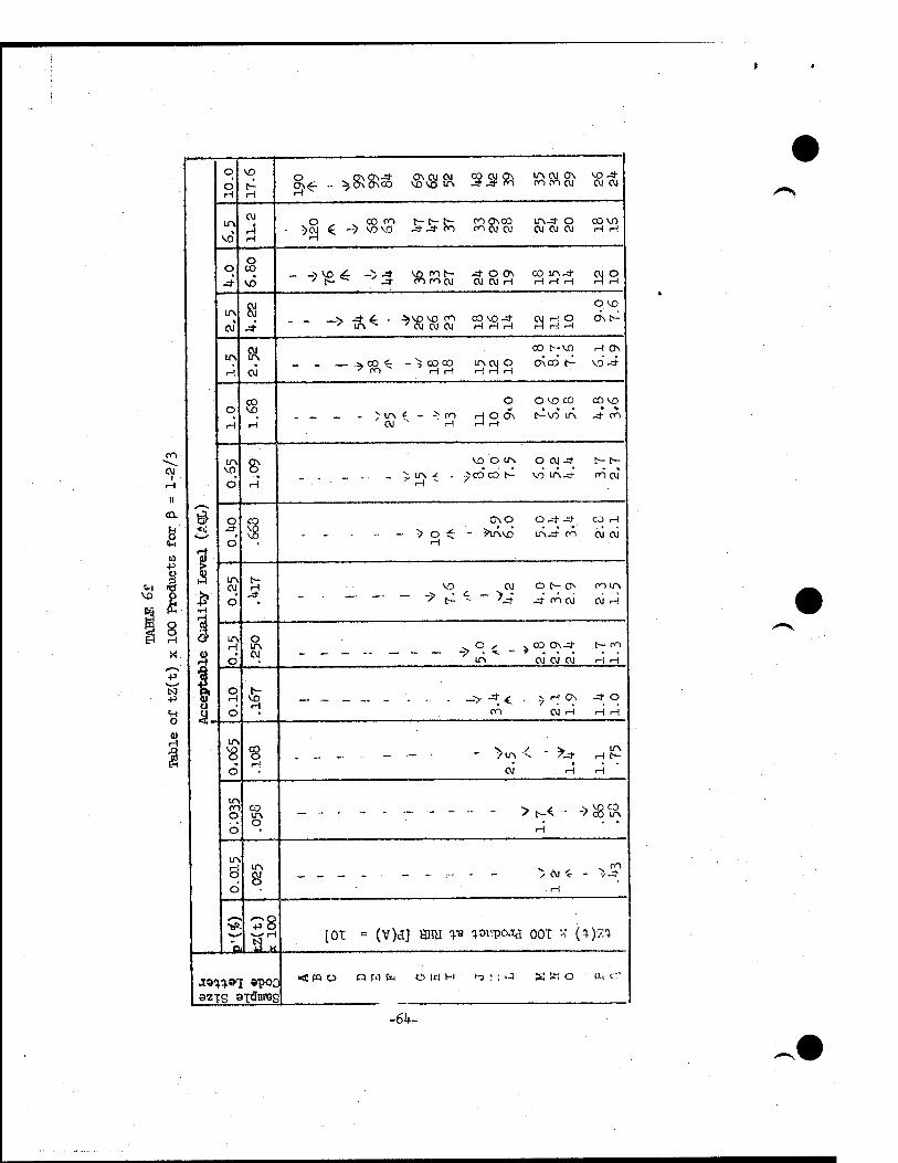
C\l I
H
II
ax
I' to •p
1-1 "Ö
8 H
•P
o
3
Ö
•H
0} H
8 3-
o
d VO
H
O _ CT\0\-=J- O\0J CM C\£- .- ^Ö\0\CO VOVO LA
CO CVJ CT\ IA OJ OS 4 4« o-itvScvj
V0 4 OJ OJ
in CM
t H H
,0, ^ co <n t-1-1>- - >Oj £ ~> VO VO -=f -* CO
m ONOO LA-* o en OJ OJ CVJ OJ OJ
covo H H
o s VO
- ->££ ->3 &££ -* o o\ oD IAJ- OJ OJ H H H H 3S
IA ft _ _. _>> -4 £ - >vo vo on CO VO^J- OJ H O H H r-i H H H
O VO
ONC^
IA
H OJ _ _ — >coi -^coco
7 m H H
CO t-VO
LA OJ O OÄCO t^ H H H
H ON
v6-=f
O
H
CO VO
H . _ _ - > IA £ - -^ CO
CVJ H
O O VO CO
rj O 6\ t^VO* lÄ
COVO • %
in VO
O H ' H ~
VO O IA O OJ -*
£co"cd i^- vo lÄ.*
t-1-
cncvj
O
d 58 VO - > O < - ^lAVo m-d- on
CO H
OJ OJ
LA
d 5
* - • — - -> ^ OJ O t-ffi
c _ > - ... '■4-. _4 oocvl
m LA
CVJ H
LA H
d o ir\ OJ _ _ _ .. — - — ^ O ^ -v CO 0\-=J
-^ . 1. - * . . .
LA CVJ OJ OJ
t— m
H H
o H d
VD H
___-..- . .. . ■
on CVJ i-H
-* o
1-i r-i
d . .- -. ■■ - - - - >LA < - >^
OJ H
LA
I-i
in on o d
CO in O
- ' - - - ->8&
LA
Ö 6
in
8 - - - - ■■ . ■- - ■- - - "> <M *
H
1 0 +»o
[01 = (V)d] SHU ** 1onpo.ta 0OT " ( i)zi
az-pg sxdnrec
, < PQ O O W fx O It! HI i-3 ' ; P X fc O dl cr
-64-

A.0
■ c
c H
r-i o o o o .* in ro
g?<r - ■> a a S g,^> 00 HCQ mm.2r Jf corn &£
» ro H
H
O ITiJ .* roro
O OWN CO CM CM
CM O CM CM
c H
00 - -> &«• ->&. 33 8 ONJ- ro
(M CM CVJ 8iS£ £9
i in '■ — "^ \$ * " "/ ro ro CM CM CVJ H £39 H
O ON H
i/
r-
N 8 H in - - - ~>^ *8I8I "339
H
38* -tf O • • t~-VD
c r
H > o H C\i ro H 3 218
Jt o o
oo co t—
co^t ITNJ*
CM
II
U
c
-\ O D ro
6 H H
CO o
■O ON ON
ro roro
t4vo in -* ro • • J- CO
U
e 10
s < < ? 8 " CO
H CM i-l -d- H
vo in-d-
J- ITN
rOCM
1 O
Ä .
1 ' A O
• UN o 0\"" lÄ
COJ- IfN
-=£.=£ CO
00 ON • • CM H
o H
•P
3* . ro
o >J- in ON
roro CM
H in • • CU H
in O
4>
■S " ■"& 57 u
V
8 8 6 °i
— - - - - vvo ro ' CM CM
t— OJ • • 3H
H
•Erl ■n O o ro
- H o
- - - •>o ro H
J- ON • • H
in ro o ..___._ - - .- ... ... O ^ _.
CM
O
/ • • H
in H O O CO ► o
o - - - - — •■ -
H - -? in
*—' v ' 1— - . N
[Or = (V)d] HHH VO q.onpOJy[ 001 - (q-)zq-
n spoo atcBtreg
<BO ficqb OtSH h> t-i J s a o f^ O'
-65-

<B
1 5
tn
S^ .._,-3 5-§ 8 ON? CO_t ON C—VO UN ßt _• _* UN_*_h
QVO _f CO
uN • VD
oo * 3 _> ON 4 ... ^ 8 ON fipK £3.2 fÖnft
00 UN CU CU
o • vg * t-
_ -§*_}£ ÄSNIV &&& CO COH cvi cvj cvl 33
irv t
cu
ro co
vo" -.- _>$<L - .^Po-ft C-UNCU
CVI CVJ CU SH"S 33
UN • H
• >£<-">$£ 8IS» _h COH HHH
o-t- - • ONt-
•S1
O • H
H UN
CU - - - ->^" -»A t—UNCO HHH
ONVO
o ONCO" H
H UN • • t-UN
CU
II
UN VD
d CO VO • ^ CO« "
CU ^sm OCO UN • • « ONt-VO
UNCU • • UN_*
£ 10
5 * o
8 • H
— .. _ - -> ^ H
00 ON N • •
- .V COCO
UNVO H • • - t-VD UN
COH
Jt CO
8
UN CU • o
UN
* ro ONUN-=j- • • •
UNI/N-t"
UNCO • • cocu
H
+>
UN H
V o co • - - - — - — ■-■■ -
t~ _r-=fco
VD ON '• • • CU H
•P
V H
* o
o CU * H.<-
UN
-->CVJ ON
CO CVI
CU UN • • CU H
irv
_ • o
CO
3 _______
CO ->H.
CU
t-H • • H H
ro O
• o
I- _ •
- - - - __..__ - - > CU
>. CO&T
>H '
UN
• °3L CO O
v0^ UN
' 'H *■
Pi
_5f = (V)__7 HHH VB q.onpo__ OOT x (q.)zq.
_9!p \&I apoo 3 ST-_~S
<|WÜ P fü) f-i _ W H h> « ^ S fe o PH G?
-66-

•rl
H I
co
II CO.
J> CO
I 1
H •9 0) O
3
- o
3 •
ir\ oo .ft*-*&S8 §§§ K3^ £$fc coco
irv3f
UN * -* si
O O O -* -* r»- .fcr ffiVft 'CVI ~ TH H
RS'ä t-CO roco
o • ft oo H
cOfOW »Si
IT» t
OJ
5 * co
o oocuvp *aQ5) ^ O <_ - > <rt ""»-* oo oo cvi
irvcvi o www 5S
ir\ r
3; ir\ — -^^. < — y oo fl*> ro (M CVJ ss»
ON CVI ON rH
o • H
co • oo 7 R - TCVI . CVI CO H «a
vo CO • ft 0\l>-
lf\ •
o CVJ _. _ -»a*- ^vguj
CO -tfVD « •
o oo • H »s)«~>ä°|
coco qcovo rH
t-CJ • •
IT« w * o
oo ro 00 • ■ — ■ — - - ■ - > m 4 — >oo
H
O -*0\ • • • CO t-irt
VO H • • Jt CO
• o 1 ^s<_
t-00 ON • • • lf\V0
row
3 • o
ro ro oo •
^0OO\ 7.tf CO
0\O • • w w
in
d s ft O
> ^ <-»s coin» • • CM H
in Or" o • o
^7 Pi •
____-.---•------ -««- T • • H H
IT
Ö c
O irv O • _.__-------
CVJ -A
•P *
[0T* = (V)<I] HHH V3 q-onpojy 00T x (q.)zq. i
■ ■"
) . <ii tq o fi H P* OWH bWhl a Wo & <y
.67-

II
<0L
S £
+»
O
3
3
!
I 5? o
3
o H ft £*--» ■RÄ8 www S5S 3§* £££ TO
UY » vo
OS
-*S* - »s§ 0 2Ä1
as* ÖFi^ SWR 3?3
o * 4 ->§ cocovo &S>£ IAOO.3- .* rn en Q IA tnevi
• CVJ
H • 3
_ v. §<- .. lA-tfvo ^ vovo IT»
.* O IA 3J* en
O t-lA meg CU
HCO «M H
IA • » VO
_ . ->SU ->#:$ vo OMA «neu CVI W cvl H 33
O • H
8! • —>v$ «-*a 00 tAH
eg cvj cvl vo IA'CO H H H
CO
vo • O
• >**- • *sias ^as
0O0O .ft • 00 VO
5 • o
o VD • " V _>33 3 300'
C\0 « » VO IA
IA Cvl
• o
8 • _. . _ _ H ■*9
IA00 O • • • CJsCO t-
V0 00 • • 1APO
IA H • o
8 VO • — . _ _ ---> h- ONO ON
•s. « • • ■J-VO t-lA
Cvl H • • .4- ro
a O
8 ■
— - - 00
IA-* • • CO cu
IA
• O
8 • - — — _ _ _ _ _ vo 00
co 00 • • Cvl H
iß & ff o 8 ■ • >2 * -
V.0.4- 7 ' •
Cvl H
• o
o • -»3* -4°.
H
Pi
438
9M I or = (V)cT| HHH q.« q.onpoja OOT x (%)2%
xsq.qa'i spoo < WO ft W 1* O W H
-68
bMri a BO On Gf I

O
4?
vo
CU
t*
CM
Vo en
O CM
n vo
o
«
o cu
IT» cvj
o
B
Jtaq48T; epoo
oös ^g\0\ir\ öS ITS -* § H öCNCö co t- irv CU CU CU CVIHHHHHH
^S4-^8S 332 8§ä ££$ RS> <n CU H H H H H
xO,/ sO OQ-* CUQCO «f\t-CO 00 CU 81 ~ ^ HP00 f^'® "^ ^v* •* «<^ H r4 H
— — - —r vox. 7o5f-t- ir\-*3- co<nv\ cu cu
--> §«->\RÄ S&rt gttSS? S3
>£*->& &äfc slSS 33
^ Näua 3S3 )«o
a
-Js. '<- ^ 00 O t-
CU 3 3 3" I--*
— ~? ir\ sVO00-=J- coos -r • • • • «
oooo t- ir\m
-> /
3 • • • •
VO *f\ Jt PO
- -»2« v o-> ir\cu / • • • -=)• cocu
JS H £ - ^VO I- ■ • • ir> CU H
CO H
69-
h)Wi4 SBO PHG?

3
9 Ö
ft S
I e
0)
§
o
to ID to
CO
4) H
CO
4
CO
ü
1
u 6)
■ä «
(D t) O M
m o
3
H
8 •H H cä
<§■
(U H
« 0)
ü
O
s 0+- -► H WM ir\t-a\ coco -=f H H OJ M4 VO ON 00
IA
••»*• o<- -»•■ H oj cimvo ÄSI& -* OJ o-| OJ m-tf
C0-* voo,
o .* ~* O*- -* H OJ f"»-* VOCOH t-O 0\
H CM OJ IA H -tfCO
IA
J-VD0O H H OJ 00 IA
IA
H ro.3- IA coo^ H H
O IA OJ co
O
H OJ m-tf iAt-q PH
IA IA H OJ
IA vq d H OJ m .* lAf- PI'S
o
d
IA OJ
d
••-» H OJ cn.* iA 00 ro H
-* H OJ cn-d- VO 0\
IT» H
d O ••*" -► rtWM -* b-
o H d
d
'•"♦ H OJ n-ilA o
■••-» H OJ m
CO o d o'•'♦" '"■"•"* H OJ
IA H O
d -"* H
1 i <u 3 H
CO ft
4> N ß
•H 10
OJ c-iiA t-g IA iOi^o H H CM OOIA
IAO O IAO O O O IAO t— IA
H
tu H ü & N
3 I» CO
O -P o <u
rH
<pqo P W I* OWH »iMrt S B O PH Cf
-70-

Appendix A
Instantaneous Failure Rate as a Life-quality Criterion.
Biis appendix describes the instantaneous failure or hazard rate
which is used as the life-quality criterion for iteos subject to the
testing procedures given in this report.
For an arbitrary lifelength distribution defined over 7- x < °°
(y is the threshold or location parameter) with c.d.f. = F(x), and
p.d.f. = f(x), the failure rate, G(x,T), at time x in proportion or
fraction (multiply by 100 if "percent" instead of "fraction" is desired)
per T time units is (see sketch),
fx. + 1!
G(X,T) = x f(y)dy _ F(x+T) -F(x) 1
T [ l-F(x) ] T R(:0 . (Al)
In Equation (Al): (i) Die integral represents the proportion of the
original items expected to fail from time x to time (x + T) and (ii)
1 - F(x) = R(x) represents the proportion of the original items expected
to survive to time x.
•71-

F(x+T) F(X)
Hence (i) /[(ii) • T Jgiven by Equation (Al) represents the expected
rate of failure at time x for the next T time units. When x = y, the
threshold or location parameter, G(/,T) is called the initial failure
rate. Since F( y) = 0, R( y) = 1,
G(?,T) = F(y + T) / T.
For 7 = 0, the initial failure rate is,
(A2)
0(0,T) = F(T) / T, (A3)
vhich is a very special kind of failure rate. But Equation (A3) is
used widely to define the failure rate. (Cf. e.g. Altm&n , Davis.;'",
-72-

Page 28
h-lOo11, Section 1 A3-2, p. 12, and Meyers12. However,this definition of
failure rate is correct if the underlying lifelcn^th distribution is
e::ponentiäl, and-incorrect for any other, distribution.
To show Jtw(ixv/e statement is so, Equation (Al) may be re-written as,
R(x) - R(s + T) 1 «(* + T) . G(x,T) = = - tl —- J- U«0
T • R(x) T R(x)
For the exponential case, R(x) = exp [-x/0 ], for x,e>0; then,
;Exponential, G(x,T) = [ l-e^* ] / T = F(T)/T, (A5)
which depends only on T and is independant of x. Furthermore, for
small values of T./0 , by use of the exponential series expansion and
neglecting terms of second and higher orders for T/ö , F(T) =
1 - e [ 'T/e ] S T/0. Tien Exponential, G(x,T) ? (T/0) / T =
l/p = X , which is often misquoted as the exponential failure rate.
(See comments on the instantaneous failure rate below).
The instantaneous failure or hazard rate (or simply hazard),
Z(".), also known as the intensity function,is the limiting value of
G(x,T) as T -» 0. Hence,
Z(x) = Lim G(::,T), (A6
)
T -► 0
which may be worked out for an arbitrary lifelength distribution by
taking such a limit. By recalling the definition of the first derivative
of a function,
Lim r F(x + T) - F(x) j = F.(x) = f(x). (A7) T - 0 T
-73-

Hence,
Z(::) = f(x)/R(x), for x £ 7 ;
= 0, otherwise. (A8)
Bie physical meaning of the instantaneous failure or hazard rate lies
in the fact that Z(;:) represents the relative failure-propensity or
failure density of an item at age x. In this report., it is adopted
as a measure of life-quality (Cf. Bo. (l)}. By its definition, Equation
(A8), since R(x) £ 1, z(x) s f(x) ft Ü for x & 7 . As U mutter of fuel,
it can be larger than unity. Thus the term hazard "rate" (uhLch implies
a proportion or fraction) given to Z(-) refers only to a "per unit
time figure, and is not necessarily a fractional number.
From Equation (A8), one may derive the original arbitrary life-
length distribution by the steps that follow [ Equations (A?) through
(A15) ] . Rewrite Equation (A8) into.-
Z(x) = F'(::) / R(:c) = - R'(x) / B(x) = - ^ [lnR(x)],
(A9)
which is,
d [In R(;0 ] = - Z(:0 dx. (/u.0)
Integrating both sides over the interval (-» , x) gives,
J7 d [In R(y) ] + ;x d [In R(y) ] = - f7 z(y) dy -
/" Z(y) dy. (All) 7
-7k-

Since for - °° < x £ 7, R(x) = 1 , or In R(:;) = 0 and Z(x) = 0,
Equation (Ail) becomes,
In R(x) = - /* Z(y) dy, for x g 7, (A12)
or,
R(x) = exp [ - t Z(y) dy J = l-F(x) for x a 7 . (A13) 7
Hence, the lifelength c.d.f. is,
F(x) = 1 - exp [ - /x Z(y) dy ] for x ä 7; y
= 0, otherwise, (Al1)-)
and its first derivative with respect to x,
f(x) = Z(x) exp [ - /z Z(y) dy ] for x fe y„ 7
= 0, otherwise. (A15)
The foregoing is true for all distributions including.
the exponential case. We now turn to our assumed mathematical model,
the Weibull distribution of the form:
ß F(x) = 1 - exp [ - (~) ] , K i 7; Ti,. ß >0;
= 0, otherwise, (Al6)
and its p.d.f.,
f(x) = ß («12 ) " eXp[-(H) ],x, 7, „,p > o;
= 0, otherwise. (A17)
In this report, since 7 is assumed to be known,Equation (AI6) and
(A17) are not used. Instead, Equations (AI8) and (A19) are referred to
-75-

throHgboirt this report. For 7 knows,there is no loes of generality by
assuming y = 0. In this case, the Weibull c.d.f. and p.d.f. are, for
x > 0, T), ß > 0,
- ß F(x) = 1 - exp t- (X/TI) ] , and (Al8)
f(x) = £ (x/n) exp [ - (X/T,) ] . (A19)
These were referred to earlier as Equations(ii) and (3) respectively. For this
Weibull model, the expression for the failure rate, by Equation (A4), is,
Weibull, G(X,T) = i B 1- 6XP K *'- )# (A2o)
The expression for the instantaneous failure or hazard rate, by
Equation (A8), is,
Weibull, Z(x) = £ (X/T1)P"1 , for x § 0, (A2l)
which was given before by Equation (5).
When toe shape parameter ß = 1, the Weibull distribution, Equation
(AI8), reduces to the exponential distribution, (see E;;uation(A5)) with
T! = 6. Also, Equation (A20) becomes Equation (A5) and Equation (A2l)
will be equal to l/S as remarked earlier. Furthermore, under the
Weibull case, both Equation (A20) for G(x,T) for any fixed T and Equation
(A21) for Z(x) can now be seen as increasing (decreasing) functions in
x when the shape parameter ß is greater (less) than unity.
-76-

Appendix B
Average Hazard Rate as a Life-quality Criterion
lhis appendix describes the average hazard rate which is useful
as the life-quality criterion for any arbitrary lifelength distribution
whether it be Weibull or otherwise.
The average hazard rate, m(x) is defined as M(x)/x where M(x) TO
is the cumulative hazard rate defined as, (Cf. Broadbent ),
M(x) = JX Z(y) dy. (Bl)
Suppose, as before, the arbitrary lifelength distribution is defined
over 7 s x < » , then the average hazard rate would be,
m(x) = - ' J* Z(y) dx for x > 7 , X y
= 0, otherwise. (B2)
Garvin made good use of m(x) for the Weibull case with 7, the
threshold or location parameter, equal to zero and devised a novel
graphical method for analysing among other things the failure data of
gas turbine blades for jet engines.
In acceptance sampling, the notion of average hazard rate is
particularly useful when the instantaneous failure or hazard rate,
Z(x), of the lifelength distribution changes monotonically in time-
such as doss a Weibull distribution with shape parameter ß other than
unity. This was seen in Example (8) of this report.
Combining Equation (Bl) with Equation (Alk), we have,
F(x) = 1 - exp [-M(x)] = 1 - exp [-x-m(x)]. (B3)
-77-

From Equation (A5), the exponential F(x) = 1-exp t-x/9] = 1-exp [-\x],
for x, B, \ > 0, one may interpret m(x) by comparing the exponential
c.a.f. with Equation (B3) and noting that m(x) is that average hazard
over the time period x such that,
m(x) = 1/6 = X. (BU)
Or inversely, we may define the hazard-breakeven time, t^ , as the
solution of Equation (Bh) for any specified value of \, thus,
T.X- = m_1(X), (95)
where m"1 is the usual inverse function of m. This was also illustrated
in Example (8).
Equation (B3) may also be re-written as Equation (B6), and Equation
(Bl) as Equation (B7), thus,
M(x) = -In [l-F(x) ] = - In R(x) (B6)
and,
Z(x) = gf- [M(x)l = m(x)+xidr [m(x)] (37)
These relationships facilitate the estimation of the cumulative hazard
rate, M(x), and hence the average hazard rate, m(x), as well as the
hazard rate, Z(x), from the failure data under any arbitrary lifelength
distribution by writing Equation (B6) in the following form:
x • m(x) = M(x) = exp [in M(x) ]
= e ln[-ln(l-F(x)) ] • (38)
-78-

The negative values for the exponent ln[-ln(l-p')] appearing in the
last member of Equation (B8) are tabulated in Table 2 of the National
Bureau of Standards Tables3 for p' = .0001 (.0001) .0050(.001) .9880
(.0001) .999to(.00001) .99999. Estimates for p' = F(x) from failure
data are discussed in Appendix B of Goode and Kao. A useful
approximation which can be derived from the logarithmic expansion of
Equation (B6), is M(x) = F(x) for small values of F(x), say 100 or
less, with two decimal places in accuracy.
A graphical method for estimating the average hazard rate, m(x)
as a function of x for any arbitrary lifelength distribution is avail-
able. The method will involve the use of Weibull probability paper of
15 the first kind mentioned in the reference (for 7 known) . After
having plotted the failure data (grouped or ungrouped) into the so-called
Weibull plot (not necessarily a straight line, since the distribution
is arbitrary)the graphical estimates of m(x) for any x may be obtained
in the manner to be described.
The reason that the Weibull probability paper can be used non-
par ametrically is the following:
. Equation (B3) giving the arbitrary lifelength c.a.f. in terms of
m(x), may be re-written as:
tol» [i^T] = -lnC-mTx7l+lnx (B9)
which is in the form of y = -a + z, an equation giving a straight
line with slope = 1 on the Weibull probability paper with the Y-intercept
being the estimate of -In t ^JJ- 1 . Since the slope of Equation (B9)
is unity, its X-intercept will also estimate In [ ^y I . Furthermore,
since the auxilliary bottom X-scale is calibrated in natural logarithms,
-79-

the estimate [l/m(x)] may be read off the auxilliary scale directly.
This procedure is illustrated by the following sketch.
= M(:0;' (if§10$)
The steps for getting the estimate of m(x) for a given value of
2 x are (Refer to Kao for scale designations of the Weibull probability
paper):
1) Choose a point X along the auxilliary (bottom) X-axis
and erect over it a vertical line cutting across the fitted
Weibull plot at point (x, F(x) ). The coordinates of
this point are in reference to the auxilliary scales.
2) Through this point pass a straight line parallel to a
line adjoining pts. = (0,1) and (1,0), both in reference
to the principal scales.
3) The X-intercept of the above straight line estimates
In (—r—y ), with values to be read off the top principal
scale. -80-

* »
♦
4) Dropping a vertical line from this X-intercept cutting A,
across the bottom auxilliary scale gives the value i/m(x),
which is the reciprocal of the estimate for m(x).
5) Repeat Steps (l) through (4) for each value of x for -which
m (x), the estimate of m(x) is desired.
It will be noted that if the Weibull plot happens to be a straight
line with slope equal to unity, i.e., the exponential case, then the
value m(x) produced by the above steps will be the same value independent
of x, a result which is to be expected of the exponential distribution.
Also the value l/m(x) read off the graph is the estimated mean life by
the interpretation given by Kao2. This latter result is also unique for
the exponential distribution. Figure 4 shows a Weibull plot given by
Dalman and Kaol6 which also appeared in Walsh and Tsao (p. 21), with
the estimate of l/m(x) for six values of x.
x^inhrs.) l/m^) (inhrs.) m(x) (^gj1^.
1 15 1,450 .6897
2 60 4,900 .2041
3 150 9,6oo .1042
4 750 16,000 .0625
5 2,450 9,600 .1042
6 4,900 4,900 .2041
Figure 5 shows a plot of m(x) vs. x for the four intermediate points.
It is interesting to note the "bath-tub" curve which is so characteristic
of the failure pattern of many electronic and mechanical components and
systems.
-81-

at CD ^ <o
I Finn T*Ti nfifn l3 i l i iTiiiilinffniiliiiffin i In i I?I i i i I i i i ill i i i^
< £ .' »'S
r- -J o
3WmiVJ XN3Dfci3d -82-

9 •*
•sm oooi / ssyrnivj NI oyvzw 39VU3AV
-83-
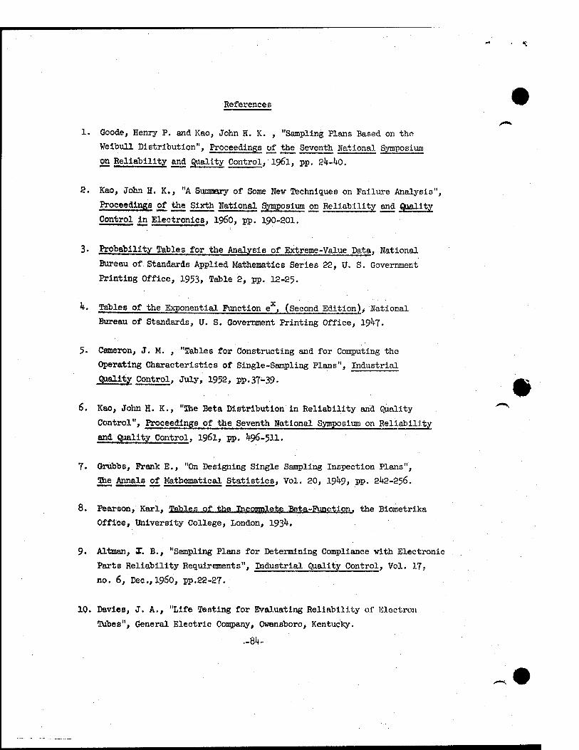
References
1. Goode, Henry P. and Kao, John H. K. , "Sampling Plans Based on the
Weibull Distribution", Proceedings of the Seventh National Symposium
22 Reliability and Quality Control, 1961, pp. 2^-UO.
2. Kao, John H. K., "A Summary of Some New Techniques on Failure Analysis",
Proceedings of the Sixth National Symposium on Reliability and Quality
Control in Electronics, i960, pp. 190-201.
3. Probability Tables for the Analysis of Extreme-Value Data, National
Bureau of Standards Applied Mathematics Series 22, U. S. Government
Printing Office, 1953, Table 2, pp. 12-25-
^. Tables of the Exponential Function ex, (Second Edition)> National
Bureau of Standards, U. S. Government Printing Office, 19U7.
5- Cameron, J. M. , "Tables for Constructing and for Computing the
Operating Characteristics of Single-Sampling Plans", Industrial
Quality Control, July, 1952, pp.37-39.
6. Kao, John H. K., "The Beta Distribution in Reliability and Quality
Control", Proceedings of the Seventh National Symposium on Reliability
and Quality Control, 1961, pp. 1*96-511.
7. Grubbs, Frank E., "On Designing Single Sampling Inspection Plans",
The Annals of Mathematical Statistics, Vol. 20, 19^9, pp. 21*2-256.
8. Pearson, Karl, Tables of ;bhe Inponrolete Beta-Function, the Biometrika
Office, University College, London, 193^.
9. Altaian, X. B., "Sampling Plans for Determining Compliance with Electronic
Parts Reliability Requirements", Industrial Quality Control, Vol. 17,
no. 6, Dec,i960, pp.22-27.
10. Davies, J. A., "Life Testing for Evaluating Reliability of Electron
Tubes", General Electric Company, Owensboro, Kentucky.
.-81+-

V
11. Quality Control and Reliability Handbook (Interim) H-108, Sampling
Procedures and Tables for Life and Reliability Testing (Based on
Exponential Distribution), Office of the Assistant Secretary of
Defense (Supply and Logistics). U. S. Government Printing Office, 196.I.
12. Myers, R. H., Reliability Testing Sampling Procedures and Tables
based on Acceptance Reliability Levals, R-56-5A, Hughes Aircraft
Company, October, 1956.
13. Broadbent, 8. R., "Simple Mortality Rates", Applied Statistics, Vol. 2,
1958, pp. 86-95-
Ik. Garvin, R. v., The Age-Dependence of Failure Rate, General Electric
Company Technical Information Series R6OFPD670, July, i960.
15. Department of Defense Technical Report No. 3> Sampling Procedures and Tab.~i.es for Life and Reliability Testing based on the Weibull Distribution
(Meanlife Criterion), Office of the Assistant Secretary of Defense.CIn- stalation and Logisticc), U. S. Government Printing Office, 196I.
16. Dalman, G. C, and Kao, J. H. K., "Determination of Vacuum Tube
Catastrophic and Wear-Out Failure Properties from Life-Testing Data",
Research Report EE Uo8, School of Electrical Engineering, Cornell
Uhiversitv, Ithaca, New York, October, 1958.
17. Walsh, C, and Tsao, T. C, (Editors), Electron Tube Life Factors,
Engineering Publishers, Division of the AC Book Compaaar, Elisabeth,
Hew Jersey, 1959«
18. Goods, Henry P., and Kao, John H. K., "Sampling Procedures and Tables
for Life and Reliability Testing Based on the Weibull Distribution (Hazard
Rate Criterion)", Proceedings of the Eighth National Symposium on Reli-
ability and Quality Control, 1962
19. Goode, Henry P., and Kao, Joh H. K., "Use of the Military Standard Plans
for Hazard Rate Under the Weibull Distribution", to be published in the
Transactions of the Sixteenth Annual Convention, American Society for
Quality Control, 1962
-85-

• «i «>•» <n
20. Military Standard - 105C, "Sampling Procedures and Tables for
Inspection by Attributes," United States Government Printing Office,
1961.
21. Goode, Henry P. and Kao, John H.K., "An Adaptation of the MIL-STD-105B
Plans to Reliabilit5r and Life Testing Applications," Transactions
of the Fifteenth Annual Convention, American Society for Quality
Control, 1961, pp. 245-259-
22. Kao, John H. K., "A Scale Estimator with Special Application to the
Weibull Distribution," Technical Report No. 6 under Office of Naval
Research Contract with the Department of Industrial And Engineering
Administration, Cornell University, 1961.
23. Keefe, G.J., "Military Standard 105 and its "C" Revision," Stimicorxiuctor
Reliability, Vol. II, scheduled for publication by Kntfinuorin^
Publishers, Elizabeth, N.J., 1961.
-86.
1 l.\ b. COVKRNWUNT PHIN'I ING OH'ICE; 1962 O-635B07