Effects of virtual reality-based planar motion exercises ...

Q
Technical Note BN-5_5 April 1968
L
ION MOTION IN ELECTROSTATIC DIPOLE FIELDS*
by
ThyagaraJa Chandrasekharan
University of Maryland
College Park, Maryland
Research supported primarily by NIH Grant NIGMS-13486, and in
early phase by NASA Grant NsG-283.
https://ntrs.nasa.gov/search.jsp?R=19680018213 2018-06-05T20:51:07+00:00Z

P£,_CEDII'4G PA_-'qE BLANK NOT FILMED.
it
TABLE OF CONTENTS
Chapter
ACKNOWLEDGEMENTS
I.
II.
Page
ii
INTRODUCTION• I
UNIQUE ASPECTS OF THE PROBLEM ................. 6
A. Transformation of Time Coordinate ............ 9
B. Minimum Distance of Approach .............. 12
C. Turning Points ............. • • • • • • • . 13
D. The Orbits ....................... 16
III. MOTION IN THE MERIDIAN PLANE .................. 20
A. Evaluation of Integrals for the Case p_ = o ...... 20
B. Different Cases of Magnitude of _/2mke ....... 25
C. The Orbit Equation ................... 30
D. Special Orbit Equations ................ 32
IV. NON PLANAR MOTION ....................... 37
A. Effect of p_ on the Roots of the Cubic Polynomial. . . 42
B. Determination of p_ .................. 44
C. _ as a Function of Time ................ 46
V. GRAPHICAL REPRESENTATION OF ORBITS AND DEFLECTION ANGLES• . . 52
A. Angular Dependence of Meridian Plane Orbits ....... 52
B. Dependence on the Sign of Initial Pe for MeridianPlane Orbits ..................... 59
C. One Case of Non Planar Motion .............. 65
VI. SUMMARY AND CRITIQUE ...................... 71
APPENDIX A. EFFECT OF ION ENERGY ON MOLECULAR ROTATION ....... 79
APPENDIX B. ELLIPTIC FUNCTIONS ................... 83
BIBLIOGRAPHY ............................. 91
iii
Figure
I.
2.
3.
4.
5.
o
7.
8.
LIST OF FIGURES
Page
Position of the Ion in Spherical Coordinates ........... 4
Translation of the Origin of Time ................ ii
Pictorial Representation of f(u) for Meridian Plane Motion. . . 23
Special Meridian Plane Orbits .................. 36
f(u) for Non-Planar Motion ................... 43
Meridian Plane Orbits for Different Values of 8 ....... 56
58Deflection Angle as a Function of Eb 2
Comparative Meridian Plane Orbits with
and Negative ..............Pe Initially Positive
62
9. Difference in Deflection Angle as a Function of Eb 2 • • • • • . 64
i0. Elliptic Coordinate Reference System ............... 74
ii. Coordinate System Used for Consideration of Rotational Effect .. 77
12. Rotational Effect of the Polar Molecule ......... 80
iv

LIST OFTABLES
Table
I. Orbit Data for Different Asymptotic Angles (MeridianPlane Orbits" p_ -- 0)
II. Variation of Deflection Angle @ with Eb 2 and e ....
III. Comparative Orbital Data for P6 Initially Positive
and Negative (Meridian Plane Orbits: p_ -- 0) .......
IV. Variation of B = (@_ - 0+) with Eb 2 and e__ .....
V. Variation of N with the Value of u3 ............
VI. Ratio of Semi-Natural Period of Rotation to Classical
Time of Action ........................
Page
54
57
60
63
70
82
V

CHAPTER I
INTRODUCTION
The motion of a charged particle in an anisotropic potential
field presents interesting features, such as non-planar scattering.
Certain aspects of this motion, eg., the bound state problem and the
scattering problem have been investigated both quantum mechanically and
to some extent classically. Before taking to our specific problem of
the classical unbound motion of an ion in the field of a fixed point
electrostatic dipole, we shall give a general background of what has
been investigated both quantum mechanically and classically for the
general problem of motion of charged particles in the field of an
electrostatic dipole.
The interaction between the charge of an electron and the
dipole moment of a polar molecule gives rise to a long distance force
which significantly modifies the electron scattering process. The
cross section for this process has been calculated for the case of a
point dipole scatterer by Altshuler I in the first Born approximation
and exactly by Mittleman and Von Holdt 2. Since the experimental
results for some polar molecules like water do not agree with these
theories,Turner 3 has tried to explain this discrepancy by considering
the possibility of a temporary capture of the electron with rotational
excitation of the molecule. Turner and Fox 4 have calculated
by a WKB method, the minimum dipole moment required for the
existence of bound states. Papers also have been published
about the problem of capture and bound states by Levy-Leblond 5, and

%
.%
2
Wallis et al 6. The cross section for slow electron scattering by a
strongly polar molecule has also been calculated recently by Itikawa 7.
A semiclassical theory of capture collisions between ions and polar
molecules has also been advanced by Dugan and Magge 8.
Turning to classical treatments, we find very few references.
The classical bound states of an electron in the field of a finite
dipole have been analyzed by Turner and Fox 9. Cross and Hershback I0
have studied the problem of classical scattering of an atom from a
diatomic rigid rotor due to an anisotropic potential consisting of a
Lennard-Jones function multiplied by [I + aP2(cos y)], where a is
an asymmetry parameter, y the angle between the axis of the molecule
and the radius vector to the atom, and P2 the second even Legendre
Polynomial. By closely following Whittaker II, and choosing appropriate
Coordinates and momenta, they have been able to reduce to seven the
number of differential equations of motion for this three body problem.
12Cross has also derived a method of calculating small angle scattering
from an arbitrary anisotropic potential, using either an impulse
approximation, or perturbation solution of Hamilton's equations of motion.
He has subsequently applied this to ion-dipole scattering, and shown
that the differential cross section in some sense approximates that
for a spherically symmetric potential given by ke___
2r 2 "
A special case of this analysis has very recently been
given by Fox 13, who has kindly supplied us with preprints of his work
14and that of Fox and Turner Aspects of the present treatment have
been given by Wilkerson 15. Suchy 16 and Spiegel 17 have separately
indicated how one might set up the Ramilton-Jacobi integrals, without
carrying out further steps. It turns out that additional insights

%
into the symmetry properties of the motion are required in order to
carry through the analysis. Aside from special cases in the books by
Loney18 and Corben and Stehle 19, our extensive literature search
has not uncovered any instance of this problem having been previously
considered to the extent that one might expect.
The problem seems to us to hold special interest because
of the fundamental and simple anisotropy of the potential, i.e. a
field having one attractive and one repulsive hemisphere with a
vanishingly small radial component at large distances. One intuitively
expects the features of this motion to be in a sense prototypical of
more general and complicatedmotions in anisotropic fields.
Thanks to the anisotropic nature of the interaction between
the ion and the dipole, the trajectory of the ion will not be confined
to a plane, except in special circumstances. In the following pages
we have developed a formalism, which we believe represents the first
analytical approach to this complex problem of the classical trajectory
of an ion in the field of an electrostatic dipole. With this
formalism, the entire trajectory of the ion can be traced.
Figure 1 surmnarizes the coordinates used in our analysis of the
problem. The proton with charge +e moves in the field of a fixed
point electrostatic dipole. As the potential takes a simple form,
when we use spherical coordinates, we represent the position of the
ion at the general time t by the spherical coordinates r, 8 and
$. The dipole moment of strength k is aligned along the z axis,
as the familiar limiting case of the finite dipole having its positive
charge on the positive side of the z axis, and its center coinciding
with the origin. The Hamiltonian H for such a system can be written as

4
Z
X
0
+e,m
Ir I
IiI
III
I\ I
\ I\ I
FIGURE I. POSITION OF THE IONCOORDINATES.
IN SPHERICAL

2 2 2
Pr P0 P_H + +
2mr 2 2mr2sin2e +
ke cos 0
2r
(i.i)
where m and e are the mass and charge of the ion respectively.
We are interested in the classical unbound motion of the
ion, as this has great significance to the general scattering problem.
For a specific problem -- the proton-water molecule interaction --
considering the polar molecule to be fixed in position and orientation
seems to be a reasonable approach. This is so, since, for the scattering
of sufficiently energetic ions, (energy E > I00 electron volts)
molecular rotation can be neglected. We believe a complete solution
of this restricted problem will prove important in treating the motion
of an ion in more general circumstances.
The scheme that we have followed in the presentation of
our calculation is as follows: Chapter II deals with the constants
of motion and certain aspects of this problem; Chapter III, with the
specific case of motion in the meridian plane; Chapter IV, with the
general case of non-planar motion; Chapter V, with a few specific
calculations of trajectories and a discussion about these trajectories;
and Chapter Vl, with a summary and critique of the dissertation.
Appendices A and B are concerned_respectively, with a review of
elliptic functions and an estimation of the ion energy above which
the turning of a free dipole (in response to the ion's presence) may
be neglected.
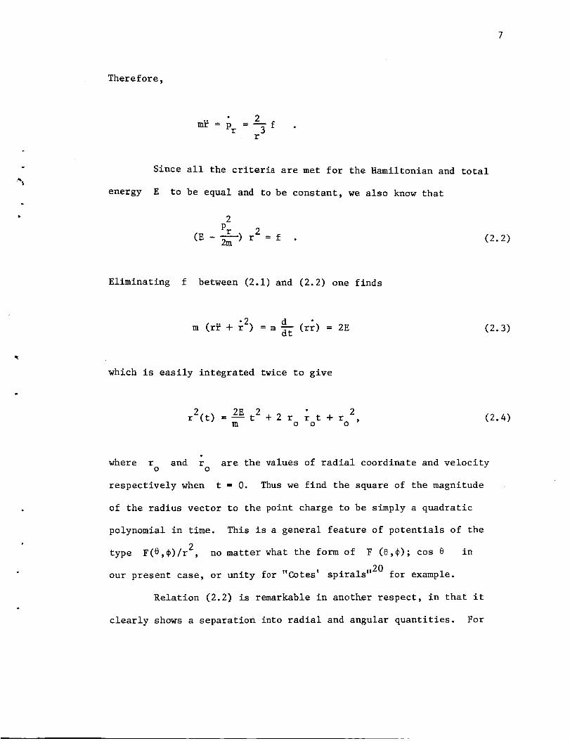
CHAPTERII
UNIQUEASPECTSOFTHEPROBLEM
b
In this Chapter we introduce the problem of ion motion in
the field of a fixed point electric dipole and discuss certain unique
features of this problem.
The Hamiltonian for the system is
I 2 . ]H = i 2 P8 P_. ke cos O2-_ Pr +_-- + + 2
r r2sin2e r
where m is the mass of the ion, e its charge, k the dipole
moment of the center of force, (e.g., a polar molecule fixed in
position and orientation) and r, e, and ¢ are the spherical
coordinates of the ion at the general time t, whose initial position
at time t = o is r , 8 and ¢ .o o o
It is clear that pc is a constant, since the Hamiltonian
is cyclic in _. We can group terms in the Hamiltonian by writing
mrH = "2_--+ f;
2 2
PS__ PC,f = 2m +
2m sin28+ ke cos 8
Hamilton's equations for the radial coordinate and momentum are
_H • Pr: _H "---- r =-- ; ---=_Pr m _r Pr = + r f
(2.1)
6
Therefore,
• 2m
m_ = Pr 3 fr
b
Since all the criteria are met for the Hamiltonian and total
to be equal and to be constant, we also know that
2
Pr r 2(E - 2_--) = f .
energy E
(2.2)
Eliminating f between (2.1) and (2.2) one finds
d (rr) = 2Em (r_ + r2) = m (2.3)
which is easily integrated twice to give
2(t ) 2E t 2 " 2r =-- +2r r t+rm o o o
(2.4)
where r and r are the values of radial coordinate and velocityo o
respectively when t = 0. Thus we find the square of the magnitude
of the radius vector to the point charge to be simply a quadratic
polynomial in time. This is a general feature of potentials of the
type F(O,_)/r 2, no matter what the form of F (8,_); cos O in
our present case, or unity for "Cotes' spirals ''20 for example.
Relation (2.2) is remarkable in another respect, in that it
clearly shows a separation into radial and angular quantities. For
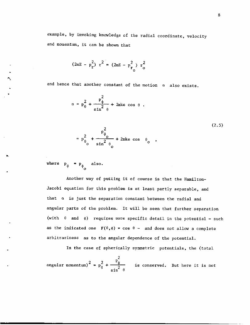
example, by invoking knowledgeof the radial coordinate, velocity
and momentum,it can he shownthat
u
2 r2(2mE - p_) r2 = (2mE - Pr ) o
o
and hence that another constant of the motion
2
2 P_= P8 + . 2 + 2rake cos e .
sln e
also exists.
2
2 P_o
= PO + 2 + 2mke cos e° ,o sin e
o
(2.5)
where p# = P#o also.
Another way of putting it of course is that the Hamilton-
Jacobi equation for this problem is at least partly separable, and
that e is just the separation constant between the radial and
angular parts of the problem. It will be seen that further separation
(with e and 4) requires more specific detail in the potential - such
as the indicated one F(8,_) = cos 8 - and does not allow a complete
arbitrariness as to the angular dependence of the potential.
In the case of spherically symmetric potentials, the (total
2
angular momentum) 2 2 _ is conserved. But here it is not= Pe + 2sin 8

%
2
2 P_conserved. Only the quantity P0 + -- + 2mke cos 0 is con-
sin20
served. As a result, the trajectory in general is not confined to
a plane.
The constants of motion are readily seen to be (i) Energy E,
2
2 P@(2) _ = Pe + 2 + 2mke cos 0
sin 9
the total angular momentum.
and (3) the z component, p_ _ of
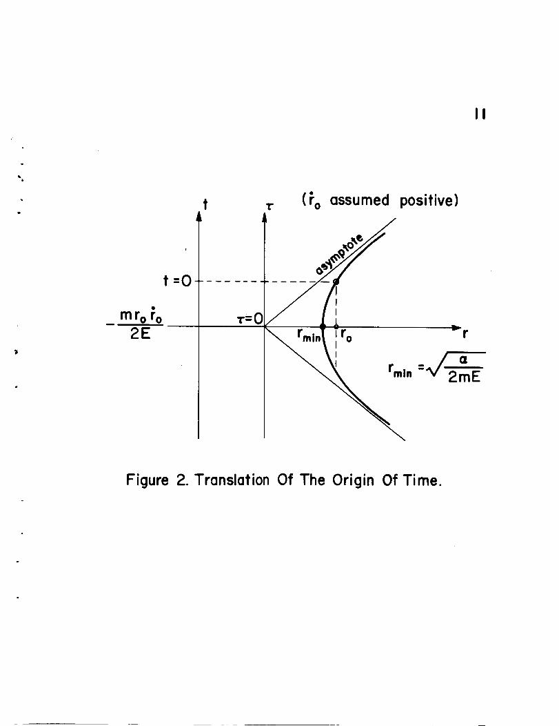
A. Transformation of Time Coordinate
2Though the expression for r (t) given in (2.4) is a very
simple and interesting one, its lack of time symmetry presents a small
barrier to several interesting conclusions.* This is easily removed
by a translation to a new time coordinate T, such that r is an
extremum (r = o) when • = 0. By simple calculations on a quadratic
2 at 2 bform r = + bt + c, one can show that t = T - --, whence thea
linear term drops out, and we have in this case
22 2E • + -- (2.6)
r (T) - m 2mE
where
T = t +
mr rO o
2E
It will be seen in Chapter 4 that this symmetrization is vital in
accomplishing the _ integration.

i0
and
o2 2= r (2mE-Pr )O
These relations immediately enable one to identify the
unbounded (i.e., scattering) orbits in terms of the constants E
and e. By a "scattering orbit", one means an orbit reaching
out to infinite distance in both time directions. In the (r,T)
plane, we require that (2.6) appear as.a hyperbola with focus onmr r
o o)the r-axis at time T = O (t = -- 2E . This is shown in Figure
2. The canonical fDrm for discussing (2.6) in this context is
2 2r T
i . 5) mfS)=I. (2.7)
from which it is clear that neither _ nor E can be negative and
still maintain the conditions for a scattering orbit. Fox 13 has
discussed the indeterminate case2 2
= E = o giving r = r . Foro
E strictly zero, and _ not necessarily zero_the earlier form (2.4)
demonstrates an inability of the orbits to reach infinity, either
in positive or negative time depending on the sign of r .o
In any
case, it is more fruitful to examine orbits for which _ > o and
E > o and let these parameters then become small in order to under-
stand the unusual cases of motion. More important, we must deal with
the entire classes of solutions for which both e and E are positive,
in order to deal with the scattering problem•
II
t
t-O
m roro2E
"L" (to assumed positive)
r o v r
rml n =,_2 almE
Figure 2. Translation Of The Origin Of Time.

12
B. Minimum Distance of Approach
From (2.5) we can write
where
= 2mE b2_ + 2mek cos ___ (2.8)
DDOO is the impact parameter
and
8__ the polar angle e at time t = -_.
From (2.6) we also know that
Therefore,
2
= 2Em r min " (2.9)
2 = b 2 + ekr min -_ _-- cos 6__ . (2.10)
This relation defines the minimum distance, rmin, in terms of
the initial impact parameter, energy, dipole strength and the angle
8_ . From (2.10), we can note the following:
(i) The minimum distance for the repulsive hemisphere,
i.e. o $ 8 < _, is always greater than zero, no matter
what the impact parameter is.
(2) It increases with increase in impact parameter, or dipole
moment k, and decreases with increase in energy.

13
(3) It is strongly angular dependent, and for a given choice
of k, E and b _, decreases from a maximum value for
O0 = o, to a minimum value for e = 180_
C. Turning Points
For the central force there is only one kind of turning point,
namely where the radial velocity r becomes zero. At this turning
point, we have for w = i/r,
dw
w = w(o), (_-_) = o for 0 = o •LLv
O
By contrast, the dipole problem possesses two types of turning
points. These are the radial turning point (r - o), and the angular
turning point for the polar angle 0 (0 = o). From (2.6), it follows
that the radial turning point is reached at zero time, and it corre-
sponds to minimum radial distance.
dr dOAt the radial turning point, (_) is zero and (_r) is infinite
dOexcept for d-_ = o.
Since
This can be shown as follows:
dr/dr = (dr/dO) (dO/dr),
it readily follows
dr dO=o if o (2.11)

14
From the Hamiltonian given in (i.i),
2 de
P0 = mr d_ '
which can be rewritten using (2.6) as
= dOP0 (_r) r (2 Emr 2 - _)
1/2(2.12)
Thus,
de PO
d-_ = r (2Emr 2 - _)1/2(2.13)
When the radial turning point is reached, r = rmin, and
(2mEr 2. - a) = o; whence (-_r8) becomes infinite, providedmln
P0
For the simple case of motion in the meridian plane i.e.,
p$ = const = o, the angular turning point can be found by using
equation (2.5). Thus,
O.
PO = ± (2rake)i/2 (2-_ke - cos 0)1/2 ; P_b = const = o (2.14)
so from equation (2.14), we can note that
o when 0 = cos -I a= (2--_7e) (2.15)
t

15
Equation (2.15) defines the angular turning point, and it can be
readily seen that no angular turning point exists when _/2mke > i.
For the more general case of non-planar motion, the angular
turning points can be found from the relation,
2 i/2
P8 = ± 2m/_e < _ p# 1 }2mke sin28 2mke cos 8(2.16)
with the substitution cos
PO = ±
8 = u, this reduces to
2mke u - u + 2mke 2mke)
(i - u2) I/2
1/2
(2.17)
which can be factored as
P0 = I(u (u - (u - I 1/2
+ 2m/_-ke - ul) u2) u3) 2; u # i (2.18)(i - u2)
where Ul, u 2 and u3 are the roots of the cubic polynomial in u.
As we shall show in the next Chapter, motion can take place only when the
value for u is between u2 and u3, the lower two of the three roots.
So equation (2.18) enables us to determine the angular turning points,
which are defined by the relation
-i -i02 = cos (u2) and 01 = cos (u3); Ul> u2 > u3

16
Wehave shownin Chapter 4, that
i > u2 > u3 and -i < u3 < u2 .
For p_ = const # o, we therefore have two angular turning points.
At the angular turning point, from (2.13), it is evident that (d0/dr)
is zero, and (dr/de) is infinity, except for (dr/dT) = o. If the
angular and radial turning points are both zero simultaneously, then
both
point.
(dr/d0), and (dO/dr) are indeterminate, at the commonturning
to the azimuthal angle
dipole potential has no
Finally we may add that there is no turning point corresponding
_, and this is due to the fact that the
dependence.
D. The Orbits
We shall now investigate how the differential orbital equation
for this anisotropic potential differs from its counterpart in the case
of a central potential.
case of motion with p_
next Chapter in detail.
For this purpose, we shall consider the simple
= const = o, which we will discuss in the
The advantage of choosing this subset of
orbits for the dipole problem is that, being entirely planar, these
orbits make the closest approach to the case of central force motion,
in which all orbits are planar. Morever, the (r,O) motion in a meridian
plane sees the full anisotropy of the dipole potential, whence we can
expect some of the differences from central force motion to emerge the

17
most strikingly. Our inquiry in this section extends to the question
of symmetry or asymmetry of spatial orbits under reflection about
the apsidal vector (vector from the origin to the radial turning
point.)
Writing the Hamiltonian for our problem as
2Pr i
H = 2-_--+_ a2mr 2
one finds from Hamilton's equations for the radial coordinate and
momentum,
m_ ---= 03
mr
Since mr2(de/d_) = ± (_ - 2mke cos 0) 1/2 ,
we write
for p_
(2.19)
= constant = o,
1/2d___ = _+ _ - 2mke cos 8) d__dr 2 dO
mr(2.20)
Therefore,
I± e)i/2 I
d2r ± qc_ - 2rake cos S)i/2 d__ ((_ - 2rake cos dr
- 2 dO 2dT 2 mr mr
(It may be observed, that though the sign of PO may change during
motion, this will not affect the second derivative of r with respect
to time). Defining w = i/r, we can rewrite this as

18
d2 0)112r _ _ (_ - 2mke cos2 2
dT m 2dI 012dw1w -_- (_- 2mke cos 7f
Simplifying and substituting into (2.19) yields the (u - O)
relation in differential form as
d2w
(_- cos e) --+--de 2 2mke
sin 8 dw
w + 2 de = o (2.21)
This relation indicates that only when e is zero at the
radial turning point, can we reflect the orbit about a vector which
will leave it invariant. Since the polar angle 8 in our problem
is already defined in relation to the dipole axis, the situation of
the radial turning point lying precisely on the dipole axis constitutes
a special case. So we may conclude, that for the dipole potential,
for this sub category i.e., p_ = const = o, we cannot generally
reflect the orbit, about the apsidal vector, except in very special
situations. On the other hand, we may note that in the case of
central force, we can always reflect the orbit about the apsidal vector,
and this is because of two reasons (i) the form of the (u - e) differ-
ential equation and (2) we can arbitrarily make the angle equal to zero,
at the turning point.
It is interesting to explore the special situations we have
referred to in the previous paragraph. When the radial turning point
occurs on the axial line, we can see from (2.21) that the orbit can be

19
°
reflected about the axial _ector._ Similarly it can be shown that
if the radial turning point occurs on the negative side of the z-axis,
we can reflect the orbit about the negative side._ For a given E
and _, there is only one such orbit; i.e., these orbits are
uniquely determined by two parameters E and _.
For the case _/2mek < i, there is an interesting possibi-
lity, that both the angular and radial turning points may occur
simultaneously. As we have shown above, this implies that dr/de
becomes indeterminate. For this case, a study of e as a function
of time, (given in Chapter 3) will establish that e(T) = O(-T).
As we know already that r(_) = r(-T), it follows that the radial
and angular coordinates are independent of the sign of time. It is
perhaps reasonable to conclude that the ion may describe some path
until it reaches the minimum distance, when both the radial and
angular velocities become zero, and then retrace its path. Since
we have assumed _ to be always positive, this common turning point,
if it exists at all, has to be in the repulsive hemisphere. We will
explore these cases in greater detail in Chapter III.
, dw d2w
Note that when e goes to -e, the terms sin e d-_ ' and cos ede 2
remain unaffected. Also we can redefine measurement of the angle e,
as the right side of the z-axis corresponding to angle e, from o to _,and the left side from o to -_. This redefinition is valid, since it does
not change the Hamiltonian.
This can be shown by redefining the z-axis. Now the potential term will
be ke cos e- 2 ; the constant _ will take a new value, but the form of
r
the equation (2.21) will be preserved.

CHAPTERIII
MOTIONIN THEMERIDIANPLANE
In this Chapter, we deal with motion in the meridian plane
i.e., p_ = const = o. This category will be comparatively simple
to understand, and we hopefully expect that one can get valuable in-
sight into certain interesting aspects of this problem, which can after-
wards be generalized to cover more general cases. Motion will always
take place in the meridian plane, whenever the initial velocity
vector and the dipole axis are in the sameplane.
A. Evaluation of Integrals for the Case p@ = o
From the Hamiltonian given in (i.i),
2 dO
P0 = mr d-_
which can be used to write the (0-_) integral" equation as
e(T)
Pe mr2(_)0 oo
(3.1)
we can change the integration variable
to rewrite (3.1) as
0 to U = COS 0 and use (2.16)
2O

21
Y
u I'2:u (2mke) I/2 lu 3 _--_ 2 _ __o 2mke u u + 2mke o
.(3,2)
q
The negative sign is to be taken when P0 is initially positive,
and the positive sign when P0 is initially negative. Though P0
may change sign, during motion, this will not affect the evaluation
of the 0 integral, and this has been shown in Appendix A.
The cubic polynomial in u can be factored so that
lu _ 2f(u) E 2mke u - u +-- > = (u2mke - 2-m_e )(u + l)(u - i)J
(3.3)
where a and -2mke ' + i i are the roots of f(u). So the (u - T)
integral equation can finally be written as
u
+ I" T
uO
du , 1/2
(2mke)i/2 _(u - a--9---)(u- l)(u + l)12mke
= It d!2E(T 2 + --_-_)
o 4E 2
(3.4)
where uT
at time T
and u are the cosines of the polar anglesO
and o respectively.
0 and 0T 0
All these roots are real, and in descending order
may be either (a/2mke, + I, - i) or (i, a/2mke, - i) according as
_/2mke is greater than or less than i. We can adopt a procedure
similar to discussions on the general motion of a spherical pendulum 21

22
I
22and the symmetrical top, for the dipole problem. As mentiened in the
last paragraph f(u) has three real zeros e/2mke, + i and - i.
With the roots arranged in descending order and labelled
as Ul, u2 and u3, the graph between u and f(u) will look as given
in Figure 3. Since f(u) has to be non negative during motion, we
conclude that _ can take only values between the two roots u 2 and
u3. Thus we see that while for the case e/2mke > i, e can take all
values from o to 7, for the case _/2mke < i, 8 can take only values
from _ to cos -I (_/2mke).
The u integral in (3.4) can be written in a standard form
I E u [lu 1I, du<> i ° du duu (2mke) I/2 f(u) 1/2 = (2mke)i/2 u3
(3.5)
The integral
so we get
I can be evaluated in terms of inverse elliptic functions 23
2
(uI - u 3)[ i/ J"?}1 Sn -I u° - u3 M sn_l/lUT - u 1/2, ,l
1/2 (2mke)i/2 u2 u3 - B_ M
(3.6)
where the notation Sn represents one of the Jacobian elliptic functions;
these functions are discussed in Appendix A. Here the arguments of
½ _ --
the functions are [(u ° - u3)/(u 2 - u3) } and {(u u 3)/(u 2 u3))½ and
the functional parameter is (u2 - u3)/(u I - u3), commonly denoted byM.

23
f(u)
a/2mek > I
a/2mek < I
II
I
-I + u
Figure 3. Pictorial Representation Of f(u) For MeridianPlane Motion.

24
The time integral in (3.4) is
z d!2E(T 2 +o 4E 2
1 -i 2E= /_--Tan (_7_ _)
So (u - T) integral fully evaluated on both sides gives
_ I/ { - u i/21 ;snl {{u u:) _M}, Sn I (u u:)/M} = ± c Tan-l(_ E T)
(3.7)
(3.8)
where
c _/mke: V2_ (Ul - u3) "
The positive sign is when P8 is initially positive, and the nega-
tive sign when P0 is initially negative.
From (3.8), we can see that the polar angle 0 can be
expressed as a function of time, provided e is known. The constant
e can be calculated from the initial conditions of the problem.
Thus we can write, as given in (2.8),
: 2mE b2 + 2me k cos 8__
where b__ is the impact parameter and 0__ is the polar angle 8 at
time T = - _. This expression enables us to calculate e, provided the
impact parameter b__ and the polar angle 8__ are known.

25
Further consequencesof our evaluation of the motion for
p_ = const = o, require someattention to the magnitude of _/2mke
relative to unity.
Case I.
B. Different Cases of Magnitude of _/2mke
_/2mke >> i.
The roots in descending order are:
u I = _/2mke >> i, u 2 = + i and u3 = - i.
Equation (3.8) with these substitutions becomes
SnI{(2rake + i
2 =c _p2 _ J
2-_e + 1
(3.9)
where •k_n_ °c is (2-'_-e'e+ 1)
As the parameter,
a/2mke >> i,
inverse sine
the constant
M = 2/(2-_eke + i), is very very small, when
we can approximate the above equation by substituting
functions, for inverse S__n_nelliptic functions. Also
c becomes equal to 1/2 so (3.9) can be rewritten as
uo+l} ilu+lSin [I" 2 - Sin-i _2 =
i Tan-i (2Ey 7_ T) (3.10)

26
Making the substitution T = -_, in (3.10) we get
(3. ii)
_°
We can use (3.11), to replace uo
U(T). Thus
in (3.10) and finally write
u : 2 Sin 2T S.n-II uI + Tan-i 2E I ]
7j_ T -1 (3.12)
We can also establish a relation between u__ and u+_ which repre-
sent the cosines of the polar angles at times r = -_ and +_
respectively. Thus from (3.10), and (3.11), we have
Sin- - 2 - 2 = ±11 / Sin- 1 .u+_ (3.13)
Application of (3.13) shows that deflection is zero for this case
i.e., _/2mek >> i. This is what we should expect, for a/2mek >> i
corresponds to very large impact parameters. Since the dipole
potential is weak, very large impact parameters will make the deflection
practically zero. By making explicit calculations using (3.12), we
can also show that the trajectory is nearly a straight line.
Case II a/2mke > i.
The roots arranged in descending order are
uI = _/2mke, u2 = 1 and u3 = -i.
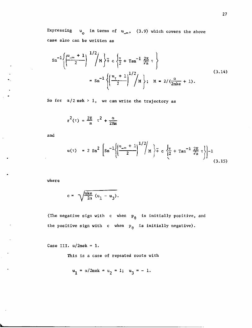
27
Expressing u in terms of u _,O
case also can be written as
(3.9) which covers the above
sn-llIU-_2 + I) i/_ 1 i_ 2E }M $ c 12 + Tan-i 7_e •
= Sn-i 2 M ; M -- 2/(2--_ + i).
So for _/2 mek > i, we can write the trajectory as
(3.14)
2(_) 2E 2 + er = --m "_
and
u(T) = 2 Sn 2 ISn- J_ -i 2E• _ -'2" M $ c ]2 + Tan 7_
k
(3.15)
where
= __ /mke
c V 2e (Ul - u3)"
(The negative sign with c when Pe is initially positive, and
the positive sign with c when Pe is initially negative).
Case III. _/2mek = i.
This is a case of repeated roots with
uI = a/2mek = u 2 = i; u3 = - i.

28
and
l( }1/2f(u) = u - l)2(u + l)
The (u - _) integral equation can be written as
uz du(u - i) _/i + uuo
._ke 2E= Tan-l-_-_-z (3.16)
By changing the variable u to u' where u', = u - i, the u
integral in (3.16) can be reduced to a standard form and readily
evaluated. Thus
j u du luz-i du'(u - i) V1 + u = u' Vu-_W'-fu o "Uo_ I
and we finally get using (3.16)
= Tanh-i 2 +_/'_ 12 + Tan-i _ z
(3.17)
So for this case of repeated roots, we have
2(_) 2E 2r : m _ + _12Em,m
and
u(T) = 2 Tanh 21 1/2_ lJ_
[Tanh-li{U-_'2+ ) , _ /_+ Tan-i 2E T!I_I
;Jc .18)
t.

29
This "degeneration" of the inverse Sn functions to inverse Tan
hyperbolic functions follows as a natural consequence of the relation
Sn(u/l) = Tanh(u) , and the parameter M = 2/(2--_ek + i) in the
above case is i. It should also be noted that (3.18) will not cover,
the very special case, where motion is only along the axial line.
For while (_/2mke) = i, in this case P8 is always zero, and we recall
from the (8 - _) integral equation, that Pe should not be always
zero, to evaluate the integral.
Case IV. _/2mek < i.
The roots arranged in descending order are
u I = i, u 2 = 2mke_ and u3 = - i.
As before expressing u in terms of u , (3.8) can beO --_
written as
sn-l, + 1 l/2/ ] (3.19)
where
a______+I )_m_e 2mekc = -- and M = 2 "
So for this case of _/2mek < i, we can write
U(T)
(3.20)

30
Wehave to note that, in this case, there is an upper bound for
u value given by _/2mke and also u__ has to be $ _/2mke.
Apart from the fact that an angular turning point given by-i
0 = cos (_/2mke) exists, the possibility of angular turnings
(occuring i or more times before u is reached) also exists.T
The number of times such angular turnings occur will depend upon
how small _/2mek is, and also when u(_) is calculated. Irrespective
of the occurence of such angular turning points, u(T) can be
correctly evaluated using (3.20).
A study of the expressions for r(_) and u(T) indicates
that for a given ion and given dipole strength, the trajectory can
be traced, provided three parameters are fully specified. These
are the energy E, the impact parameter _ and the asymptotic angle
e_ . (If b__ is known in magnitude and direction, the sign of
P8 (initial) can be fixed). Before we close this section, we can
make a passing reference to the case of /_ being negative. Since
the solution for the time integral is (i/_) Tan -I {(2E//_)_},
we find that the trajectory remains unaffected, whether /_ is
positive or negative.
C. The Orbit Equation
We can also write the orbit equation for motion in the
meridian plane. We know from (2.12) that
= d8 _ 1/2Pe (_)r (2Emr 2 _)
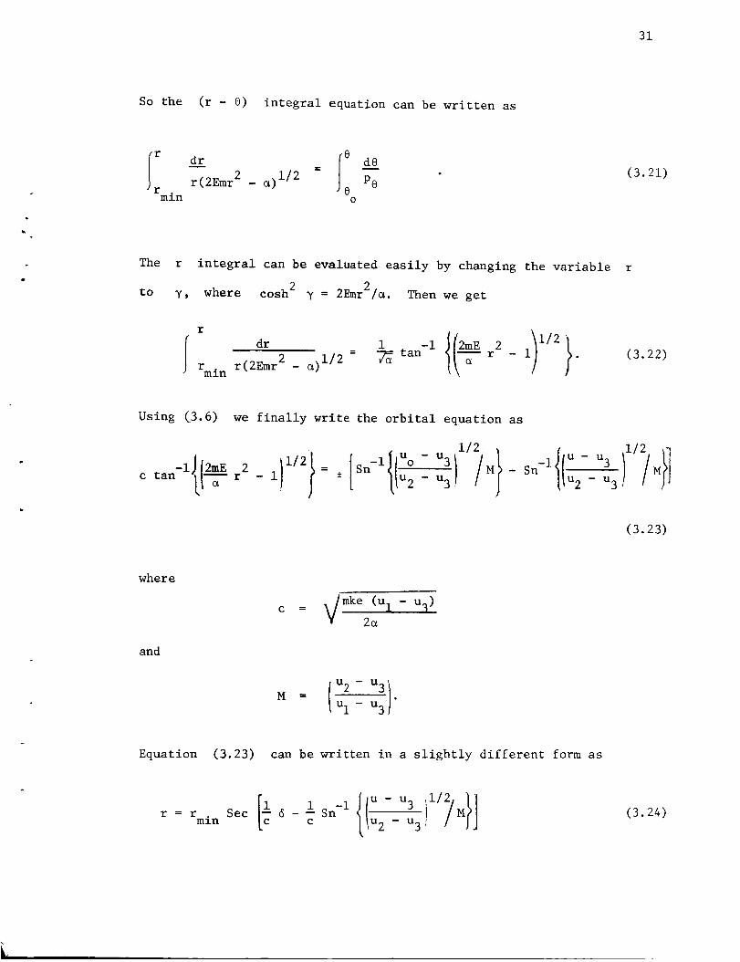
31
So the (r - e) integral equation can be written as
r dr I e d__eer(2Emr2 _ e)i/2 = Permin 80
(3.21)
o
The r integral can be evaluated easily by changing the variable r
to y, where cosh 2 y = 2Emr2/_. Then we get
r )}rmin r(2Emr 2 _ _)i/2 = 7_ tan-i r - i .(3.22)
Using (3.6) we finally write the orbital equation as
c r sn_lliUo _ u3 MI _l_lU- u3 )i/- i)i/2i= + [ [I_2 u311/i " -Sn flu2- u 3 iMl]
(3.23)
where
and
Vmkec = (Ul u3)
2_
M
Equation (3.23) can be written in a slightly different form as
r = rmin /.
c _u2 - u 3(3.24)
32
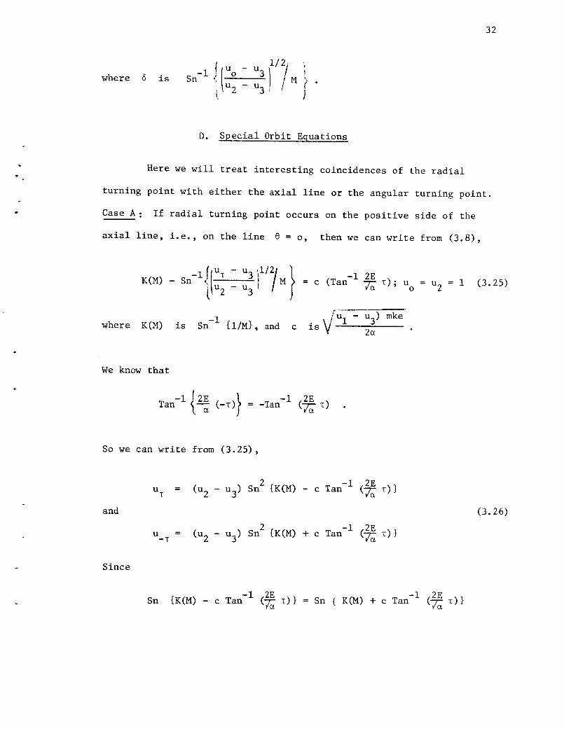
where 6 is -iSni u3 i• J
D. Special Orbit Equations
Here we will treat interesting coincidences of the radial
turning point with either the axial line or the angular turning point.
Case A : If radial turning point occurs on the positive side of the
axial line, i.e., on the line 0 = o, then we can write from (3.8),
where1 - u3)
K(M) is Sn -I {l/M}, and c isV u
mke
2_
=u2= 1 (3.25)
We know that
Tan-i { 2E (-T)} _Tan-i 2E-- =
So we can write from (3.25),
and
uT
= (u2 - u3) Sn 2 {K(M) - c Tan-i (2E7__)}
u__ = (u2 - u3) Sn 2 {K(M) + c Tan -I (2E7_T)}
(3.26)
Since
Sn {K(M) c Tan -I 2E (7_ _) }- (7_ _) } = Sn { K(M) + c Tan -I 2E

33
Wefinally get
u = u (3.27)T --T
Similarly when the radial turning point occurs on the negative side of
the axial line, we can write from (3.8),
= Tan-l( 2E T) u3 -iSn-i I__ M c 7_a ; u = =
/ °(3.28)
and from (3.28) it readily follows that
U _ UT -T
So we can conclude, that when the radial turning point lies on the axial
line, the orbit can be reflected about the axial vector. Figure 4a
illustrates these orbits. We can also write the orbit equations from
(3.24) as
1 Sn-i ; u = u 2r = rmi n Sec -c o= i.
(3.29)
and
mr Secl SniIr1 u31 <3.3O>min c ilu 2 - u 3 o
Case B: If the radial turning point coincides with the angular turning
point, then we have u = u 2 = a/2mek. We can find u__, from theo
(u - _) integral equation. Thus we can write;
U ---- U0
34
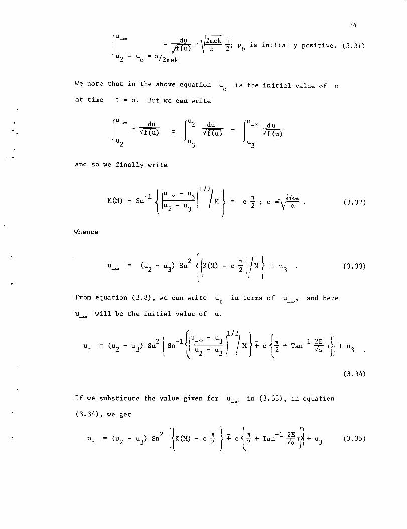
du _2_ek _-/--_ = 2' Pe is initially positive. (_°.31)
= a/2mek
We note that in the above equation
at time r = o. But we can write
u is the initial value of uo
u u 3 u
and so we finally write
- M = (3.32)lu2- u 3
Whence
ci; c --V-7-.
u_= = (u2 u 3) Sn 2 I,K(M) - c _ M + u 3 (3.33)
From equation (3.8), we can write u in terms of u and here
u__ will be the initial value of u.
uT = (u 2 -u3 ) Sn2 [Sn-i iu/__- u3 ____ 2E_ U2 _33 M $ C [2 + Tan-i 7_- T + u3
(3.34)
If we substitute the value given for u__ in (3.33), in equation
(3.34), we get
u r = (u 2 - u 3) Sn 2 K(M) - c_ $ c + Tan-1 2E-_a + u3 (3.35)

35
Only if P0 is initially negative, i.e., P8 at time
get
U% = U T
= -_ we
Also we know that r = r T. The only way in which these conditions
can be satisfied is that when the ion reaches the common turning point,
it should retrace its path. From (3.24), we can write the orbit equation
for the above case as
Sec [i K(m) i Sn-i u - u 3 (3.36)
r = rmin [ c - c u 2 _ u3)
where
Figure 4b illustrates these orbits. These retracing orbits are
curved because of the non-aentral nature of the dipole field; for
central field problems, one is familiar only with straight-line
retracing orbits (zero impact parameter) for the scattering problem.

o° 36
90 °
k
180 °
(a). Reflection Of Certain Meridian Plane Oribits By Dipole Axis.
90 °
90" I 90 °
180 °
(b). Meridian Plane Orbits Retracing T.heir Curved Path After Reaching TheirCommon Turning Points. (i.e. _=0,8-0).
Figure 4. SPECIAL MERIDIAN PLANE ORBITS.

CHAPTER IV
NON-PLANAR MOTION
In this Chapter we deal with the motion of the ion when
This means that, in general, the trajectory will not lie in a
To express e as a function of time, we have to evaluate
both sides of the integral
U±_
U0
$ du
(2mke)i/2 _ 3 ________ 2u 2mke u - u + 2mket
T=+oo= d_
2rake "_=o I
(4.1)
For this we have to factor the cubic polynomial
2P
{u3 a 2 _ 2___ke}f(u) = 2mke u - u + 2mke
We adopt the method given by Birkhoff and MacLane.
and u3 be the roots of f(u). Then
f(u) = {(u - Ul)(U - u2)(u- u3)} _ {u 3 2mke
24Let
2u -u+
uI , u2
2mke
2
_h_2mke }
(4.2)
37

38
Equating coefficients of like powers of u on both sides of the
equation (4.2), we get
-
c_
Ul + u2 + u3 = 2mke ;
u I u 2 + u 2 u3 + u 3 uI = -i
2
p_ -
Ul u2 u3 = 2mke
(4.3)
(4.4)
(4.5)
From (4.3), we have
u2 + u3 -- 2mke uI (4.6)
•Also from (4.5),
u 2 u 3 =
2
:P_- _ _,1
i_mk---_ ! uq(4.7)
Therefore
(u2 - u3) =
or
t
(u2 - u3) = 4m 2 2 + mke u I mke Ul + Ul mkee
Solving the two simultaneous equations in u and2 u3
1 }1/2uI(4.8)
given by (4.6)

39
and (4.8) we write,
u2 2 _- Ul + 2 4m2k2e2 mke uI mke
I 1/22 2p_ i
+ Ul mke uI (J
(4.9)
and
i I _ ! i{ _2 2_i _Ul- - -- + mk_e u I mkeU3 2 2m_e Ul _ 4m2k2e2
2 2p l1I12+ Ul mke Ul )
(4.10)
We can write it in the above way, because if the negative root in
(4.8) is taken, only u 2 and u 3 will get interchanged and this
is immaterial.
To complete the factorization we have to determine uI.
Since uI is one of the roots of the cubic polynomial f(u), we
can write
3 2 2
2 rake u I - au I - 2 mke u I + _ - p_ = 0 (4.11)
The square term in (4.11) can be eliminated by making the substitution,
u_ = d + (4.12)2mke 3±
With the above substitution, and rearrangement of terms (4.11) reduces
to
22 3
d3-d( _ +li - _ _12m2k2e 2 t 108m3k3e 3 3mke + 2mke(4.13)

40
Equation (4.13) can be transformed still further to obtain simple
trigonometric or hyperbolic solutions. To effect this transformation,
we substitute
he' = d ; h = ) 12m_ 2e2 +(4.14)
in (4.13) and then multiply both sides of the resulting equation by
n -
3/[ i
c_ +
12m2k2e 2
(4.15)
With these operations (4.13) reduces to
34e '2 - 3e' = f; f = _
108m3k3e 3 3mke
2
+_It2mke 2
12 3/2
. 12m2k2e 2
(4.16)
The solution for
given in (4.16).
Thus if
e' will depend upon the value of the constant f
f is >. i,
e' = cosh [(i) cosh-1 f ] (4.17)
If Ifl is less than i, the solution is
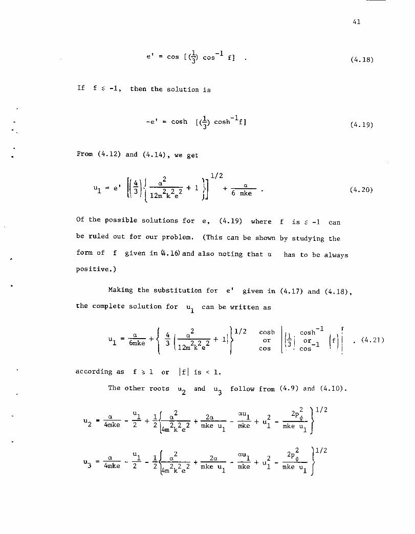
41
(_) -ie' = cos [ cos f] (4.18)
If f _<-i, then the solution is
-e' = cosh [(_) cosh-lf] (4.19)
From (4.12) and (4.14), we get
2 1/2
u 1 = e' _'. 12m2k2e2 6 rake(4.20)
Of the possible solutions for e, (4.19) where f is $ -i can
be ruled out for our problem. (This can be shown by studying the
form of f given in _.i_ and also noting that _ has to be always
positive.)
Making the substitution for e' given in (4.17) and (4.18),
the complete solution for u I can be written as
I ( 2 i}i12cosh4 _ + i or
Ul = 6mke + -3 12m2k2e 2 cos
cosh-i r
(li-3! °r-i fcos I
(4.21)
according as f _ i or Ifl is < i.
The other roots u2 and u 3 follow from (4.9) and (4.10).
u2 - 4mke
2 _Ul 2 ] 1/2Ul if _ 2e 2 2p_ ,
2 + 2 [4m2k2e 2 + mke uI mke + Ul mke uIJ
u3 - 4mke 2 }1/2Ul ! I 2 2_ _Ul 2 2p_mke u I2 2 m2k 2e2 + mke u 1 mke + Ul -

42
As a check, we can also show that
as p_ _ o, uI ÷--2mke '
u2 + 1 and
i
u 3 ÷ - i;
i.e., we obtain the very same roots that we got previously when we
considered motion in the meridian plane.
A. Effect of p_ on the Roots of the Cubic Polynomial
From (4.16) it is evident that for the case p_ # o, the value
of f will be more than for the case p_ = o. It follows easily from
(4.21) that u I will be greater than _/2mek, which is the value it
will take when p_ = o. Again regarding the roots for the case
p_ # o, it is evident from 4.22, that u 2 should decrease below the
value it will take when p# = o, and u 3 will increase above the
value it will take when p_ = o. So
u 2 < i; u3 > -i .
The cubic polynomial f(u) will look like Figure 5a or 5b or 5c,
p 2 is less than _, or equal to _ or greater than _.according as
For motion to take place f(u) must be positive, and one can see
from Figure 5, that u has to lie between u2 and u3. It is
evident from these figures that the effect of pC being non zero is
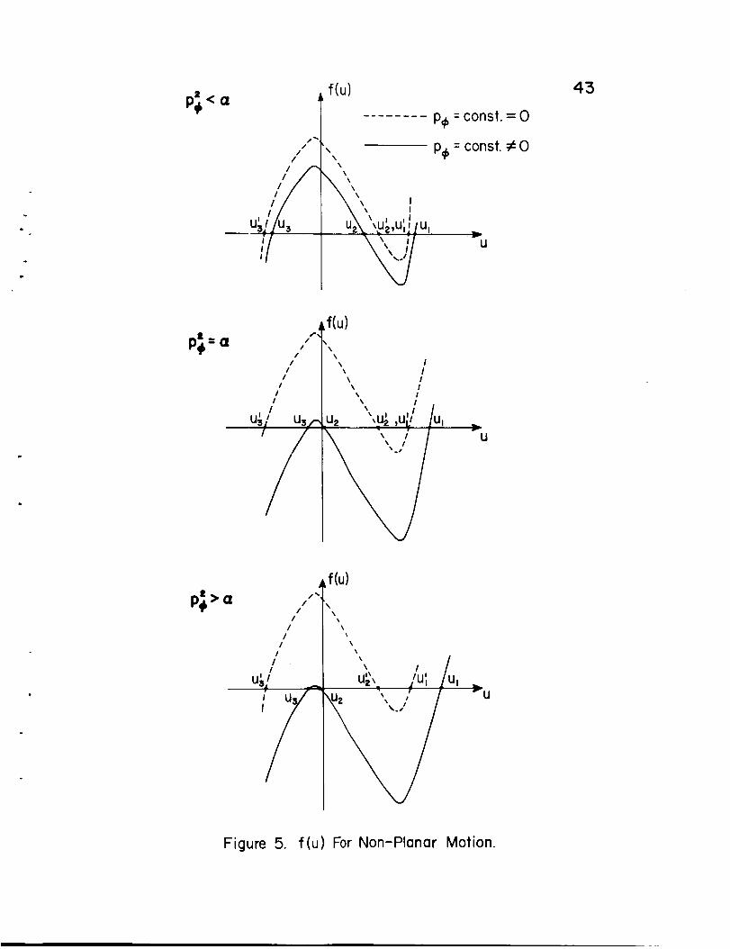
J
P÷f(u)
/ \/ \
\\
!
"u u,\,ul,u',
p@=const. = 0
p@= const. #=0
/UlU/
43
d
//
I/
/I
I/
I
/
,,[(u)\
,, /', I\ I
u, ',u_,,u;., /u,\ _', ,;I r
U
/%q
II
II
II
/I
I
f(u)
\
\
\
\
\
u_ ,/ui ijUl I
\u, , ,, / r u
Figure 5. f(u) For Non-PlanarMotion.

44
to restrict the range of value for 0. Thus
01 .< 0 .< 0 2 ; (01 = cos -I (u2)
-i
O2 = cos (u3)
and it is more than 0 °.
and it is less than 180°).
B. Determination of p_
The roots Ul, u 2 and u 3 can be determined provided p_
is known, p_ or the z component of the total angular momentum
is given by
P_ = _3 (r ×mv),
where _3 is unit vector in the direction of the dipole axis. We
can determine p_ from the initial conditions of the problem. Thus
if b be the initial impact parameter and V, the initial velocity
at time • = -_, then
p_ = E3 . (_ x m_). (4.22)
The components of-+
v at time T = -_ will be
where
y and
_ sin e__sin ^= _ sin 0_o° cos __oo_i,_-_) __ooE2and
(4.23)
_i' _2' and E3 are unit vectors along the coordinate axes x,
z respectively, ___ and ___ are the polar and the azimuthal

45
angles indicating the position of the ion at time • = -_. So-+
p_ can be determined if b, the impact parameter is fully
specified in addition to specifying e__ and
With the roots completely evaluated, e
as a function of time _.
can be expressed
u
where
I= (u2 u 3) Sn 2 Sn -I M $ _ + Tan-i 2E- c _ + u3 .
(4.24)
mke (u I - u3)c =, 2_
and
M
u 2 - u3
uI - u 3
and
Ul> u 2 > u3.
(The negative sign with c is for the case Pe positive initially
and the positive sign for the case Pe negative initially. Here
after for convenience we will consider only Pe positive case.)

46
C. 0 as a Function of Time
We have already seen that P¢ is conserved, and from the
Hamiltonian (i.i),
t
8H $ P¢
8P0 mr 2 sin28
Therefore,
2 sin28PO = mr (4.25)
So the (0 - T) integral equation becomes
10( ) ITd¢ =
Po0-=0
aT
mr2(T) sin2O(T)(4.26)
2sin O(T) required in (4.26) can be expressed in a simple form, by
making suitable substitutions.
Thus we note that,
2
sin 8(T) = (i - u )(i + u ) (4.27)
Let
-iSn
u - u3 I
M I - c_ be
J= y (4.28)

47
and
2ETan-i 7_ T = T (4.29)
With the substitutions given in (4.28) and (4.29), and using (4.24),
(4.27) can be rewritten as
sin28(T) ={ (I+u3) + (U2--U3)Sn2 (y-CT') } x
{(l-u 3) - (Uz-U3) Sn2 (y-cT')} .
(4.30)
The variable T can be changedto
integral equation (4.26) reduces to
T' defined in (4.29) and the
_(_) -- $__
-i 2E
aT v
{(l+u 3) + (u2-u3)snZ(y-cT ')}{(l-u 3) - (U2--u3)Sn2(y--CT ')}
(4.31)
The integration variable T' can be once more changed to T" where
y -- CT ! = T", (4.32)
and (4.31) can be rewritten as

48
_(_) = ___
-i 2E
y-c Tan 7_ _ d_"
I iluu¥+2- . J--u3 J , Ij- 3 )
(4.33)
Let
u2-u 3 u2-u 3-- = b (4.34)
l_u3 = a; l+u3
Then
_('r) = __oo
y c Tan -I 2E 1 Ii i d_" a + b .(4.35)
(l-u_) (a+b) c_ (i- 2z") (i+bSn2z'' )
_, + _--
With the substitutions for a and b given in (4.34), (4.35) can be re-
written as

49
b
P_ 1
_(_) = ___ - _ 2(i--u3)
y-c Tan -I 2E
(4.36)
2(i$-u3)
y- c Tan -I 2E
7f rc_
¥+ _
d_"
l+bSn2T ''
This is equivalent to writing
_(_) -- _ +__ 1- (l-u3) I
l-aSn2T") LZ(I+u3) J0 l+bSn2T'
-i 2E
c Tan 7_ Td_-a_n_"/_+u_Tan-i 2E T
l+bSn2T" J
(4.37)
The above integrals are of the form
Iul du0 l-B2Sn2u '
where B2 can take positive or negative value. These are known as

50
incomplete elliptic integrals of the third kind in Legendre's
canonical form, and the solution is
u
Iul - E (Ul,B 2) for [-_ < B2 _] (4.38)
du
0 l-_2Sn2u < "
The exact form which the function H(uI,B 2) will take will depend upon
which one of the six cases given underneath is valid.
Case i 0 < -B 2 < K
Case ii K < -B 2 <
2
Case iii 0 < < < B < 1
Case iv 0 _ K2 < 82 < K
82 2Case v 0 < < <
Case vi oo > B2 > i
1u2-u 3
Here K2(M) = (--).
ul-n3
So knowing the roots Ul, u 2 and u3 of the cubic polynomial,
(4.37) can be evaluated to give _ as a function of time _. Thus
[
P_ I i c_
_(T) = ___ + (l-u3){2(Ul-U3)mke}i/2 [ (l_u3) H(y +-_ , _2 = a)
1+
(l+u 3 )H(y+ _, - lq2 = b)
-p_
(l-u 3) _imke (Ul-U3)1(l-u 3)
-1 2E B2 = a)H(y- c Tan _ "c,
1 -1 2E
+ (l+u3) N(y- c Tan _ _,- _2 = b)
(4.39)

5]
The _ (uI, B2)
Byrd and Friedman.
functions for different cases are all _iven by25
o

CHAPTER V
GRAPHICAL REPRESENTATION OF ORBITS AND DEFLECTION ANGLES
P
In this Chapter we first discuss in sections A and B a few
specific calculations of trajectories for motion in the meridian plane
and then show in section C a special case of non-planar motion:
2
= p_ with Uo = 0.
A. Angular Dependence of Meridian Plane Orbits:
UT
We know that the equation
u3 M$ c _ + Tan -I -_ + u3
enables us to calculate uT, and consequently trace the trajectory,
provided u__ and the initial sign of Pe are known. The above
equation illustrates that for a given impact parameter the trajectory
is strongly angular dependent, in the sense that it depends upon tile
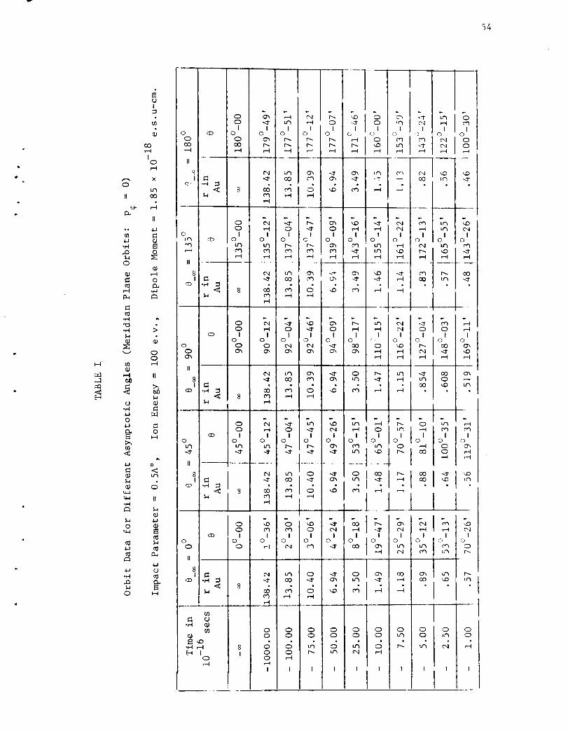
initial value u_ . Table I gives the values of r and 0 at differ-
ent times for different choices of 0__, for the case of motion in
O
the meridian plane. (We have chosen an impact parameter of 0.5 Angstrom
and an ion energy of i00 electron volts. The dipole moment of water
10 -18molecule has been taken to be 1.85 x e.s.u. - c.m. units; p@
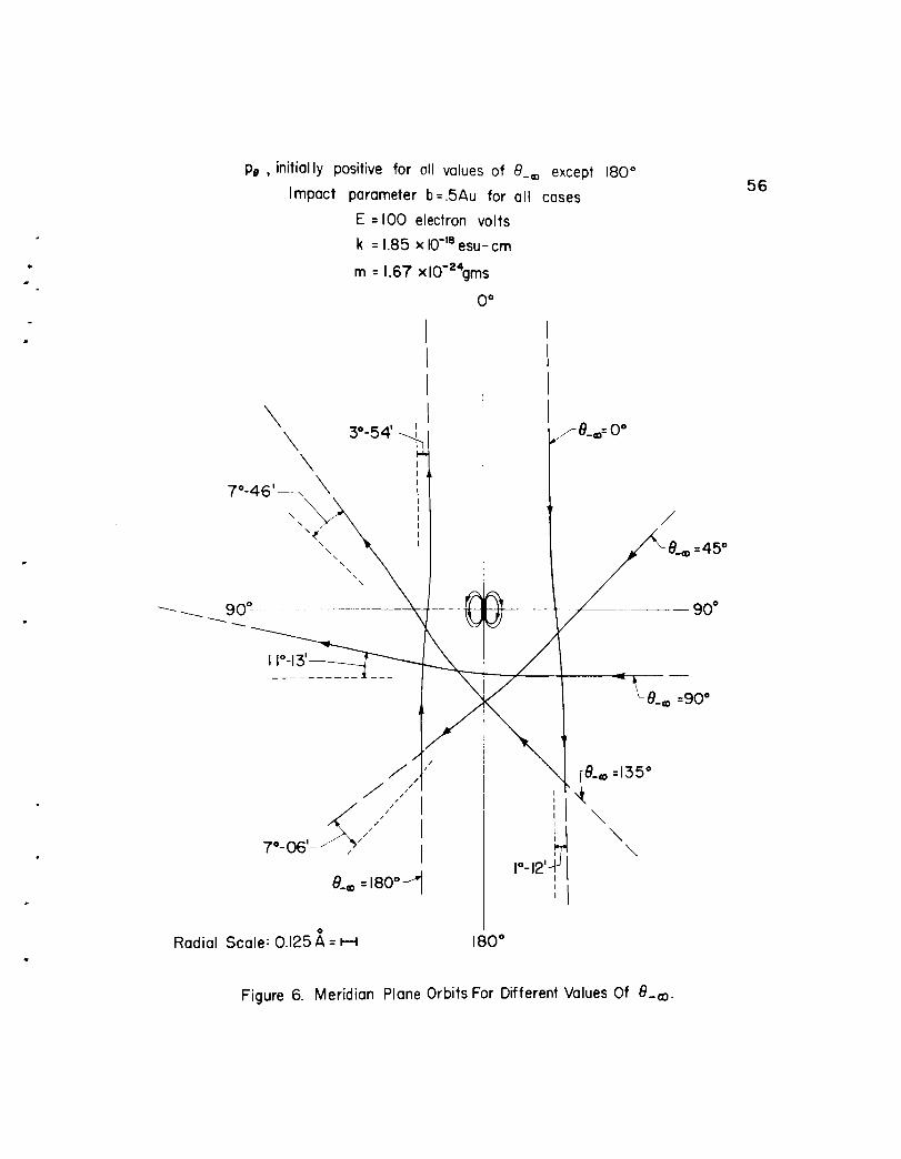
is initially positive for all @__ except for 180 °) Figure 6 gives
the meridian plane trajectories of the ion for these angles @
52

53
equal to 0 °, 45 ° , 90 o , 135 o and 180 °. One can see from figure 6
that, at large distances from the force center, the orbits are nearly
straight lines which is what one would expect. Also when the ion
is near the force center, it curves inwards, if it happens to be in
the attractive hemisphere, and curve outwards when it is in the repul-
sive hemisphere.
Table II gives the angles of deflection, @ = 180 ° - (9_o- 0+._),
for different values of Eb 2. (Pe is initially positive for every
case except for 9__ equal to 180°). A plot of deflection angle @
versus Eb 2, for different asymptotic angles e__, is given in Figure 7.
Both the figures 6 and 7 illustrate that, for a given Eb 2, the
deflection angle @ is maximum, when the ion is initially on the
equatorial line, and minimum when it is on the positive side of the
axial line, i.e., 9 is 0°.
of the ion is greater when e
It is also seen that the deflection
is 135 ° , than when it is 45 ° .
Similarly, @ is greater for 9 equal to 180 ° , than for
equal to 0°. Figure 7 also shows how the angle of deflection falls
with increase in Eb 2.
o
m
I
00;--I
IO
xO
II 00
U
H 4-1
O
cl o
_ 00
m ,--t
_-t U
•,-.t _
0
o
4-1
q-I
U,_ II
0 _
ml4-1
00
II
II
o
¢._
II
8_I
CP
OO
II
8I
OL_
II
8I
(D
OO
II
8I
CD
OO
IO
OCO
OO
IO O
OO
O IO
O
OO
CD I IO
U_
°l8
OO
CD IO
O
,_ 8
U•,-I Q.I
q,lEi,.o•,'_ ,-I 8
E.-I I I0
,----I
Oh
Io
Oh
c',l
cO
,--II
o
¢q,-.I
¢',I
oo("'l,-I
¢'.I
Io
0Oh
"-I"
00¢q,-'4
O,l,-II
0
u_
...I.
00¢q,-4
T_c,'l
Io
_q
o,I-.1"
crl
00
000,.-I
I
LqI
0
a0
D
o'Ir..-.c_,--4
LqO0
0I
0C_I
tr_O0
oq
0I
0
O0
c_
"oI
oc',l
LqO0
C_,--t
00
00
I
0 --.I" 0 .q
I I I I I I ° I I0 0 ) 0 0 0 0
°
•"1"1I I I I I I
O O O O O O
I _ _1 i
i
O '_O C_ _
, ioI I l , I ° IO O c_ O O
C_ 00 O _D r_ CO
i
O'_ _ O _ L_ ,-.1" 00C_ O'_ L_ ...1" _ U_ O
• • • ' • 00
O O O O O O
o °o
0 "...1" 0 CO
,-.-t
0 c,,I I N _ c'q o I
I I I I I IO O O O O O
I
O "--1" O I O'_ 00 O'_ U'_
,--t
0 0 0 0 0 0 0O O O O Lq O
• •
I I I I I I I I
Io
O_
,-4
?©
0",
,-4
,.0
I©
Cb
r-..Lt_
00

55
Zi-4
Zorj
o
oo0
II
8I
o
u'he_
i" p
8I
.,-4 _
CD
@
o
fl
?I
@
II .....
•_ _
@
o
II
8I
•,.-4 _
°,4
Io
o
Io_0
I0
oo
o
w
P0 , initially positive for oll values of 8__ except
Impact parameter b=.5Au for all cases
E =100 electron volts
k = 1.85 x 10-ueesu- cm
m = 1.67 xl0-_4gms
0 °
180°56
\I
3°-54' _
\
7°'46'_
"-.. \ '
90 °- "'"" "_
////
06 _, "
z //
//
I /
7 °-
8_®=180°-4
/
_/-e " °
_ °0GD
/
&® =45 °
90 °
/
-- f
//
\
1°.12'',_I
II
e._ =135°
\\
\
°
Radial Scale: 0.125 A = H 180 °
Figure 6. Meridian Plane Orbits For Different Values Of 8-_o.

57
TABLE II
Variation of Deflection Angle @ with Eb 2 and
Eb 2
ev-(Au 2)
units
f
i 8-oo=00
0+
8_=45 °
0+
12.25 3o-54 ' 11°-43 '
16.00 2o-32 ' 9o-52 '
20.25 l°-42 ' 8o-20 '
25.00 l°-12 ' 70-06 '
36.00 00-36 ' 5°-18 '
49.00 0°-18 4o-06 '
64.00
i00.00
144.00
3o_14,
2o-i0 '
lO-32 '
0_oo=90 °
0+
19°-53 '
16°-15 '
130-24 '
e_oo=135 °
0+
12°-15 '
i0°-24 '
90-06 '
8_=180 °
0+
17° -45
8°-00
5°-24 '
400.00
900.00
196.00 l°-09 '
256.00 0o-54 ' i°-18 ' 0o-55 '
324.00 0o-44 ' l°-03 ' 0o-44 '
3o-06 ' 2o-15 '
2o-12 ' io-35 '
io-40 ' io-ii '
11°-13 ' 7o-46 ' 3o-54 '
8o-09 ' 5o-45 ' l°-55 '
6o-08 ' 4o_22 ' 0o-33 '
4o-47 ' 3o-24 '

A
(/)
IJJnr
LLI
®
LLI-J(__Z
Z0
l--
bJ--ILLl,lC]
2O
18
16
14
12
I0
8
6-
4-
2-
0
=180 °
=45 °
p@,initally positive for all Jvalues of 8_=oexcept 180°
1 I I I I20 30 40 50 60 80 I00 200 30O 400
Energy x (impact parameter)=; --[Eb=] = eV
FIGURE 7. DEFLECTION ANGLE AS A FUNCTION OF Ebz.
58
I I I 1 I600 800 I000

59
B. Dependence on the Sign of Initial Pe for Meridian Plane Orbits
The expression for u indicates clearly that the value
of u depends on the initial sign of Pe " So for the same Eb 2
and e__, we will in general get two different trajectories, which
correspond to Pe being initially either positive or negative. It
should be noted that this is not so when e__ happens to be either
0° or 180 ° . When e_= is 0°, then Pe has to be initially posi-
tive, while for the case of e__ equal to 180°' Pe has to be
initially negative, and so for these cases there is only one orbit
for a given Eb 2. (There is also the trivial case of motion along
the axial line corresponding to Pe being always zero.) Table III
gives the (r-e) orbit data, both for Pe initially positive and
negative. Figure 8 gives both the trajectories for each one of the
asymptotic angles e_=, namely 45 ° , 90 ° and 135 ° . The orbits for
P0 initially negative also demonstrate the tendency to curve in-
wards when the ion is near the force center, in the attractive hemis-
phere, and curve outwards when the ion is near the force center on the
repulsive hemisphere.
6O
B
I--II--I
E_
O
II
oo
O
OC
,..-I
.H
.;-I
qJ
"H4-1
Z
_J
-H
O
,-I
.;-I.I.J._.1
Ou,q
4-1
4-1.;-I
O
QJ
.,-I
t_
0
0I
,-4I0_-4
x
II
Ill
O
Cl
d00
I
@
0
%u'3
II
0
Et
4-1Um
%
II
8I
o
U
8I
o
II
Q
0
o_
0
CL._U_OC_
_>_
08
U)O
O
,HcD4J
U_OC_
cJ
•_ 
61
t
ou_
II
8I
CD
CD
OD
.M
I_, -M
O
_ OI I I
o
o") _ _ -...1- _ i.c"1 0
I I ° I I i I I I I0 O 0 O _ O 0 O
[
m-.I C',I t.n O u'_ I._ OI I I I I I I
0 0 _} 0 0 0 0
C_l 0 CO _D I._ I._ ",1"
.... _ _
t'_ _ _ ,-'II I I I I
O) 0 0 0 0C_ (30 r-_ r_
C_ c_ oo
Z
Z0
c_ s,J I Ic_ o o
:> -.-ro "_ IO CD _ oO'_ O., .M c,_
II O ,'4
8I
1
-Hc_ 4-I
o _,
II 03O
q) l
.M
! Io o
u_
O O'_ o(3O I'-I O
O
o oO
T.n bI I I
o
i--I ,-4 r-I
I I I I .,.-ko o o o o
, ? mIo o o
c_ o_
° I Io
_ r,, _, ;., _ 7,, _, _,, ;.O c'_ r,_ c_ t._ c'_ _ _
I I I I I I I I I0 0 0 0 0 0 0 0 0
',_ CO _ _ I-'10 00 00
m-I ,.-I
t._ _ O
00• _ ,_
%.- _, , o
o o o
_0 (30 C_
C_ c_ 00
c_
0 c_ ,-_ 0
° I I ! I I Io,.o % _ T-., %
•,,4" ,--I o')
I I I
o o _u'3 t_
O O O OO _ O
m4 c',,I
7.. _ _•,-1" O ,-_
I I I I0 0 0 0
o
Io
_oI I
o o(30 r_
0 _ 0 0r_ 0 0
,-_ 0 8
0 -,.1" 0 t._ C_lO_ _ O0 -,.1"
,-.-t

Impact parameter b=.5Au for all cases
E =100 electron volts
k = 1.85 x IO-mesu-cm
m= 1.67 x I0 -24 gins
0
\
I 1°'56'__
\\
\\
\
//
78_® =45 °
p, init. neg.
8_® =90 °Po init neg.
62
90 °
/-8_= =90 °Pe init. pos.
8_© = 155°_Pe init. neg.
\\
0
Radial Scale: 0.125A= H
180 °
Figure 8. Comparative Meridian Plane Orbits With Pe Initially Positive
And Negative.
63
t
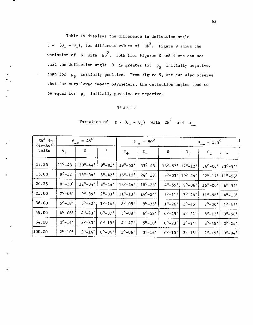
Table IV displays the difference in deflection angle
6 = (@_ - 0+), for different values of Eb 2. Figure 9 shows the
variation of 6 with Eb 2. Both from Figures 8 and 9 one can see
that the deflection angle @ is greater for Pe initially negative,
than for Pe initially positive. From Figure 9, one can also observe
that for very large impact parameters, the deflection angles tend to
be equal for P0 initially positive or negative.
TABLE IV
Variation of 6 = (@_ - @+) with Eb 2 and @_=
Eb 2 in
(ev-Au 2)
units
e__ = 45 °
6
12.25 9°-01 '
16.00 5°-42 '
20.25
i00.00
I
0+ } 0_
11°-43 ' 20o-44 '
9o-52 ' 15o-34 '
8o-20 ' 12o-04 '
7o-06 ' 9o-39 '
5o-18 ' 60-32 '
3o-44 '
e = 90 °--co
e__ = 135 °
@+ @_ O+
19°-53 ' 33o-45 ' 13o-52 ' 12o-12 ' 36o-06 '
16°-15 ' 24 o 18' 8o-03 '
4o-59 '
i0o-24 '
90-06 '13o-24 ' 18°-23 '
22o-17 '
16o-00 'I
11o-56 '
I
23°-54' i
4o-47 '
I 3o_06,
Iii°-53' i
I
6°-54'!
4o-10 '
l°-45't
I
25.00 2°-33 ' ii°-13 ' 14°-24 ' 3°-ii ' 7°-46 '
36.00 l°-14 ' 8o-09 ' 9o-35 ' l°-26 ' 5o-45 ' 7o-30 '
49.00 4o-06 ' 4o-43 ' 0°-37 ' 6o-08 ' 6o-53 ' 0o-45 ' 4o-22 ' 50-12 ' 0°-50'!
,-i
64.00 3°-14 ' 3o-33 ' 0°-19 ' 5°-10 ' 0o-23 ' 3°-24 '
2o-10 ' 2o-14 ' 0o-04 ' 30-16 ' 0o-i0 ' 2o-15 '
i i
3°-48 ' 0°-24 'i
2°-19' i 0°-04'i
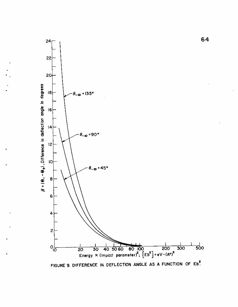
64
p
22
2O
¢/)(D
18"lO
e.-°w
(D_, 16e-
e'-0
14
'10
.C
12(3c-
t,.4)
IOA
4-
1
i 8®
II
mL
=135 °
8_ m =90 °
6- \
- \4--
2--
I-I0 20 30 40 50 60 80 I00 200 300 500
Energy x (impact parameter)=; [Eb =] =eV-(A°) =
FIGURE 9. DIFFERENCE IN DEFLECTION ANGLE AS A FUNCTION OF Eb =.

65
C. One Case of Non-Planar Motion:
In this section, we shall investigate the interesting case of
2
= p_ with Uo = O. Then
f(u) -- {u 3 _ 22mke u -u} - u(u - i) (u - u3) ; u 2 = 0. (5.1)
where
-._ 2
Ul = 4mke ÷ _16m2k2e 2+i
and
u3 = _- 6m2k2e 2 + 1
From (3.8), we can write
uT = - u3Sn2 K(M) - c Tan-i -_ / + u3 (5.2)
where
M = Ul _ u3 , K(M) = Sn -I / Ul _ u3 j
and
/!mkec = \ _ (uI - u3).

66
Onecan readily see from (5.2) that
Wecan also investigate the
= U •UT --T
motion for this special case.
When p_ is positive, from (4.35) we can write
_+= - ___ =i
2c (i - u3)
CTI
K(M) + _--
CTI
K(M) - _--
dT"
2 I!
(i -aSn • )
(5.3)
+2c (i + u3)
c__!
I K(M) + 2
K(M) - c--l_2
d_"
(i + bSn2_ '')
where
- u3a -
i - u 3
and
- u 3b =
l+u 3
For large impact parameters,
will be much smaller than i
u3 is approximately equal to 2 mke/_, and
in magnitude. So we can use the Binomial

67
approximation and write
i = I + aSn2_'' + a2Sn4T''i - aSn2T'' (5.4)
and
ii + bSn2_''
= 1 - bSn2T'' + b2Sn4T''
With the above substitutions (5.3) can be reduced to
c_K(M)+
f _
71 2¢+_ - ¢ _ = a !- 2 Sn2T"dT"
(i - u3) K(M) - c___2
(5.5)
c__l_
I K(M) + 2+ b' Sn4"r"d'r ''
KCM) - c_.._._2
where
!
2i 2u3
c (i - u32) 2
and
iDT _
c
2
u3
(i - u32) 3

68
Since the functional parameter, M equal to -u3/(u I - u3) , is very small,
we can write
and
MSn2 ,, = sin2 ,, _ M4 _" sin 2T" +_ sin2(2_ ")
Sn4T,, sin4_ '' - M(sin3T"COST")T'' - M sin4T '' cos2_''
(5.6)
where we neglect higher powers of M. Using the values given in (5.6)
for Sn2_'' and Sn4T'' and evaluating the integral on the right side of
(5.5), we finally get
_+_ - ___ = 21 - u3
- a' + _) _ - cos 2 K(M) sin c -_ cos 4 K(M) sin 2 c_
+ _ (M) + -- cos CK(M)- _)cos (2K(M)
+ b' - c_ - _ cos 2 K(M) sin c
M I<K <K(M) + _ __ sin4 c_ _}
+ _ in 3 c_) sin 3 _2K(M) c_
(5.7)

69
Applying (5.7), we can calculate the difference in azimuthal
angle _ = (_4_ - __=), for small values of u3. Table V gives
the difference for different values of u3. Wefind that this differ-
ence tends to 180°, when u3 decreases in magnitude. From table V,
we can infer that this difference is most probably 180°, and that
the departure from the value of 180° is most likely due to the
various approximations we have madein the evaluation of the integral
in (5.5). Wehave adopted the above method of evaluation, i.e. expanding
the Sn functions in terms of sine functions and the parameter M,
because exact evaluation of the integrals in (5.5) becomesdifficult.
For example the integral
IK(M) + _c_
2I - Sn2_'d _'
C_
K(M) - _--
can be evaluated* as
M c_ +
sin-i ISn (K(M)+ c_) 1
i - Ms in2 u du
o
I sin-If Sn(K(M) -_)I i- _ - Msin 2 u du
o
(5.8)
In Byrd and Friedman's "Handbook of Elliptic Integrals for Engineers and
Physicists", these integrals have been evaluated in page 191. Also see
page 18 of the same book.

70
Though
Sn K(M) + = Sn K(M) _-
it is not clear whether the two integrals in (5.8) will cancel out.
TABLEV
Variation of y with the Value of u3
u3
- .1926
- .1623
- .1231
.1615
.1396
.1096
.2385
.1937
.1404
yO : (_+_ _ ___)o
182 ° - 04'
181 ° - 28'
180 ° - 45'

CHAPTER6
SUMMARYANDCRITIQUE
In this Chapter, we summarizeour findings and propose possi-
ble avenues of further investigation of this problem.
Wehave first of all demonstrated that for all i/r 2
potentials, irrespective of their angular dependence, the square
of the radial vector is a quadratic in time.* For our specific
problem, we have identified an important constant of motion,2 2 2
= Pe + (p_/sin 8) + 2 mke cos 8, in addition to E and p_.
Wehave also shown, that by suitable translation of the origin
of time (i.e., the time T = 0 when the ion is closest to the
force center) we can obtain a symmetric quadratic expression in
2 T2time, r = (2E/m) + e/2Em .
Further, we have investigated in depth the comparatively
simple case of motion in the meridian plane with a view to under-
standing someof the complexities of the general problem. Wehave
expressed the polar angle O as a function of time, by meansof the
Jacobian elliptic function Sn. It has been shownthat the general
*This was first demonstrated by T. D. Wilkerson (15) and independentlygiven in a recent preprint sent to us by K. Fox (13).
71

72
meridian plane orbit can be defined in terms of three parameters: 0
(the asymptotic polar angle), energy E and the impact parameter b
A few representative figures corresponding to motion in the meridian
plane have been given. These figures exhibit such interesting details
as the angular dependenceof the orbits, the effect of the sign of
initial P0 on the orbits and deflection angles, the variation of
deflection angles with Eb2 and finally the expected tendency for the
trajectories to curve inwards in the attractive hemisphere and outwards
in the repulsive hemisphere.
Wehave also discussed another interesting aspect of this
problem, namely the turning points. Wehave shown that we have two
types of turning points, the radial and the angular, for the dipole
problem. For the case of motion in the meridian plane, we have
further shown that the orbits in general cannot be reflected about
apsidal vectors. (Special exceptions have been noted in Chapter 3.)
Wehave indicated that a particularly interesting exception arises when
the two turning points merge; the ion retraces its curved path after
reaching the commonturning point.
Wehave also solved the general case of non planar motion
and obtained an expression for (_+= - __=) in terms of H(u,B2)
functions which are types of incomplete elliptic integrals of the2
third kind. Finally we have discussed the interesting case of _ = p_
with u = O.o
This problem can be investigated further regarding certain
aspects like the effects of polarizability, finite size and rotation

73
of the polar molecule on the trajectory of the ion. Regarding polariza-
bility, we can regard the ion-polar molecule interaction as classical,
if the sumof the Van-der Waal'sradii of the ion molecule pair is less
than the impact parameters of interest. Then we can write the ion
molecule potential energy* as
2e
ke cos 8 oV(r, e) =
2 - -- (6.1)r 2r 4
where
r = ion-molecule separation distance
8 = angle between the positive end of the dipole axis and
the vector r.
= average electronic polarizability of the polar molecule.O
We note that (6.1) presupposes that the polarizability of the polar
molecule does not depend upon the relative orientation of the molecule
to the ! vector. (We assume that the polarization effect is isotropic).
We can conclude that the effect of this altered potential energy is to
cause less e deflection of the trajectory.
As regards the second effect, namely the finite size of the
dipole, we can choose elliptic coordinates** to describe the position of
the ion. Thus we can define two elliptic coordinates e, and q as
shown in Figure i0,
*J.V. Dugan, Jr. and J. L. Magee have used the above potential energy (8).
**K. Fox and J. E. Turner have analysed the bound state problem in the
field of a finite dipole, using elliptic coordinates (9).

74
\\
\\ ,.
.co.s_.T*y.___':CONSTANT--_I .._
_ -L_ -q\
17=+I _
.l-e
r,
T f'_ =o
Figure I0. Elliptic Coordinate Reference System.

75
where
rI + r 2
2£ ; (i .< _ ._ _)
and
and
and
and
rl=
r2=
2_ =
rI - r2
2£ ; (-i .<n .< i)
distance of the ion from charge +e
distance of the ion from charge -e
length of the dipole.
(6.2)
With these new coordinates the Hamiltonian is
H = e2- 2 2 _ i pen
1
+ (i - n2) p2 + p_ {e2_n i
--+
(6.3)
where pe, _ and p_ are all the momenta conjugate to the coordinates
e, n and _ respectively. The Hamiltonian given in (6.3) will serve as
a starting point to carry out analysis of unbound ion motion in the field
of finite dipole, particularly for orbits having small rmi n (_ .2A°).
We can deal with the rotational effect, by noting that rotational
excitation involves transfer of many quanta of rotational energy even
at large impact parameters. So we can use a classical description of the

76
molecular rotation. The rotational motion can be investigated by re-
writing the Hamiltonian as
H = TR + T.lon + V(r,Y)
where TR, T. and V(r,Y) are the rotational kinetic energy of thelon
dipole, the kinetic energy of the ion and the interaction potential
energy respectively. The interaction potential energy can be written
as
V(r,¥) = ke cosy2 (6.4)
r
where y is the angle between the dipole axis and the radial vector of
the ion and can be expressed by the following relation
cosy = cos9 cosg' + sin9 sing' cos(4 - 4') (6.5)
9' and 4' are the polar and the azimuthal angles of the dipole axis.
Let us assume for simplicity that the mass distribution of the
dipole body is such that two of the principal Moments of Inertia are
equal (I) and the third (about the body Z-axis) is zero. The familiar form
2 2 2 6EI (_E) + ($E) sinof rotational kinetic energy thus reduces to
where E denotes Euler angle. Figure Ii illustrates the simple trans-
formation required to then make use of the angles 9' and 4' employed
above;
= 4E 4'9E 9'; = 7/2 +
Therefore, the rotational kinetic energy becomes
TR 2 ( ) + ($' sin 2 (6.6)

77
3.I Z
\\\\_o
Y
Figure II. Coordinate System Used For Consideration OfRotational Effect.
78
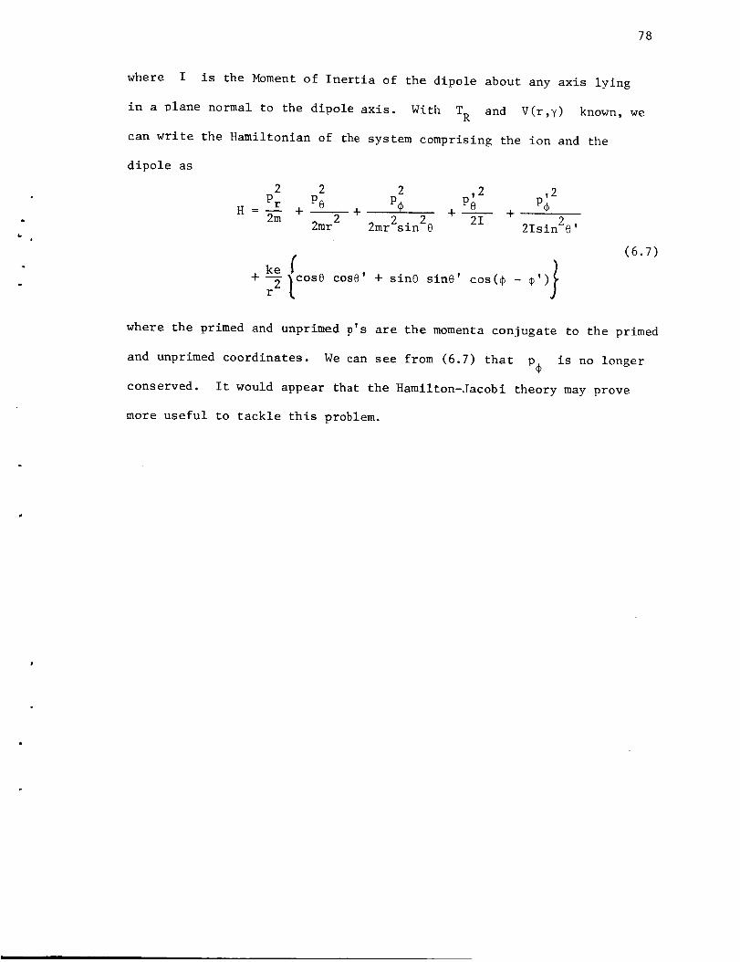
i
where I is the Moment of Inertia of the dipole about any axis lying
in a plane normal to the dipole axis. With TR and V(r,y) known, we
can write the Hamiltonian of the system comprising the ion and the
dipole as
2 2 2 2 ,2
Pr P@ P_, P@ P_H =-- +--+ " +-- +
2m 2mr 2 2mr2sin2@ 2I 2isin2@,
+-_ os@ cos@' + sin@ sin0'r
(6.7)
where the primed and unprimed p's are the momenta conjugate to the primed
and unprimed coordinates. We can see from (6.7) that p_ is no longer
conserved. It would appear that the Hamilton-Jacobi theory may prove
more useful to tackle this problem.

79
APPENDIXA
EFFECTOFION ENERGYONMOLECULARROTATION
Wecan estimate the ion energy above which the rotational
effect of the polar molecule can be neglected in the following way.
From Figure 12a,
c = e_E sin e (A.I)
where c is the couple acting on the dipole of length _ due to
an electric field E caused by the ion, e is the charge and e is
the angle of rotation of the dipole. The characteristic period of rotation
of the polar molecule can be found, by regarding the oscillation to
involve small angle only. Since
d2ec = I -- (A.2)
dt 2
where I is the Momentof Inertia of the polar molecule about its
axis of rotation, we have from (A.I) and (A.2)
__ e_Ed2e +-_- 0 = 0 (A.3)dt 2
whence the natural period P is given as
=_2IP ¥ egE (A.4)
From the figures of the orbits that we have drawn, we note
that the deflection of the ion from a nearly straight line trajectory
starts practically when the ion is at a distance of 1.5 times the min-
imum distance rmi n from the force center. So we can regard a distance

o
\_', B_
\
8O
(a). Couple Acting On The Polar Molecule.Field Lines Rougly Parallel From Ion.
2d dv
(b). Classical Path Of The Ion.
FIGURE 12. ROTATIONAL EFFECT OF THE POLARMOLECULE.

81
equal to 2rmi n as the effective range of E. (The electric
field will be down to a fourth of its maximum value, when the ion is
at 2rmin.) We can calculate P by substituting an average value
of E in (A.4).
eE ~
average 2r2.rain
• P -_
e2£
The classical period of action is given by T, where
W -_
4rmi n
V; v is the velocity of the ion.
(A. 5)
So we get
Moment of Inertia of the water molecule is I, where
(A. 6)
2I ~ i to 3 × 10-40 gms - cm .
10 -28The factor e2£ is roughly about 25 x . So we get
P i0-i-- -_ (6.5 x )VT
(A.7)
Since the velocity v is _2_m , we can calculate the
ratio _ for ions of different energy. Table 6 gives the value ofT
P/_._2 for ions of different energy. The ratio P]2 can be regardedT T
as a measure of the applicability of our formulation. The higher this
ratio, the greater is the justification for neglecting the rotational
effect of the polar molecule. Thus our calculations are well founded

82
for kilovolt protons in a molecular dipole field of this strength,
while molecular rotation would surely have to be considered for
proton energies of 10eV and below.
b
TABLE VI
Ratio of Semi-Natural Period of Rotation to
Classical Time of Action
P
Energy of the 2
v in cms ion in e.v. T
4.5 x 10⁷
1.4 x 10⁷
.45 x 107
i000
100
i0
15
~4.5
~1.5
83
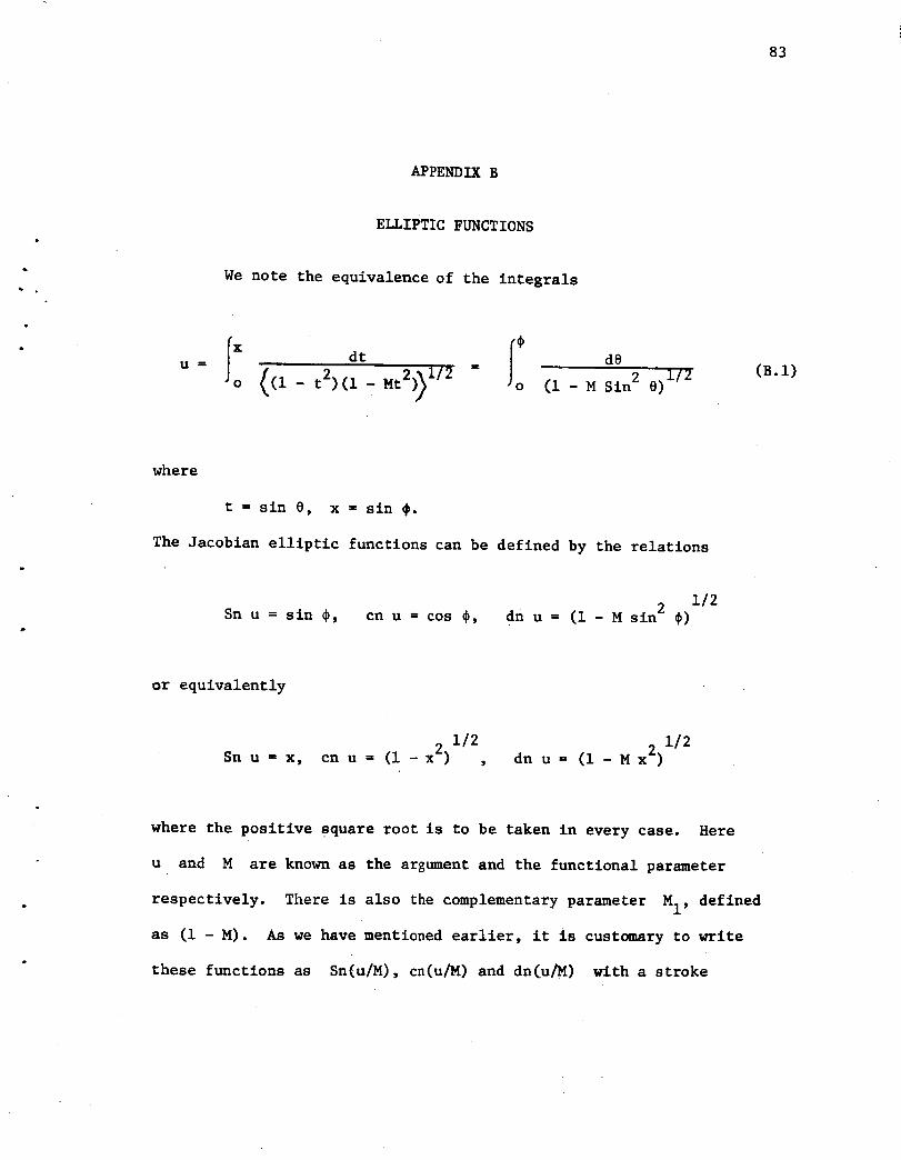
APPENDIXB
ELLIPTICFUNCTIONS
Wenote the equivalence of the integrals
I- i .I'x dt
o /_l - - Mt2_1/2 o%, -/
d8
(i - M Sin 2 8)1/2(B.I)
where
t = sin 8, x = sin #.
The Jacoblan elliptic functions can be defined by the relations
Sn u = sin _, cn u = cos _,
112dn u = (i - M sln 2 #)
or equivalently
1/2 1/2Sn u - x, cn u = (i - x2) , dn u = (i - M x 2)
where the positive square root is to be taken in every case. Here
u and M are known as the argument and the functional parameter
respectively. There is also the complementary parameter MI, defined
as (i - M). As we have mentioned earlier, it is customary to write
these functions as Sn(u_), cn(u/M) and dn(u_) with a stroke

84
separating the argument and the functional parameter. The three
Jacobian elliptic functions are single-valued functions of the
argument u and are doubly periodic. Wehave also two other quantities
called K(M) and K'(M) defined by the relations,
I IK(M) = _ dO(1- Msin 2 8)I/2 ; iK'(M) -- i _ d0
o o (i - Mlsin2 0)1/2
(B. 2)
These are the real and imaginary quarter periods.
We list some of the important properties of these functions
which we have used elsewhere.
Sn (u/o) = sin u, cn (u/o) = cos u, dn (u/o) = i.
Sn (u/l) = tanh u, cn (u/o) = dn (u/l) = sech u.
Sn (-u) = - Sn u.
Sn {2K(M) - u} = Sn u
cn{K_M)-u}Sn u = dn{K(M)-u}
iSn(u/M) = sin u - _ M cos u (u - sin u cos u) ;
'(B.3)
M very smallJ
Now we shall show that irrespective of the change in sign of
P8 during motion, the expression for
initial p@ .
u T will depend only on the sign of
Case 1 P8 is initially positive. Let us evaluate uT at some
time %, such that % < _3 i Then P8 will always remain positive. We
have already seen in Chapter 3, that we have to evaluate the integral I,

85
where
I - duI = + ,/2 mke _f(u)
and the negative sign should be taken when P0 is positive, and the
positive sign when P8 is negative. So we have
I By
U oo
-du i- _ 2E_2 mke Jf(u) = 7_e {2 + ran-i 7_ T}'
which can be rewritten as
lul Iudu T
J2 mke _f(u) -
u u 3
du i _ -i 2E
¢2 mke Ff(u) = 7_e {7 + tan 7_};
whence
uT = (u2 - u3) Sn 2 {(6 - c8)} + u3, (B.4)
where
sn_l u co - u3 u2 - u_
_3 ; M = Ul u3
and
-i 2E= {7 + Tan 7_e_}

86
and
mke (uI - u3)c = 2a
t
Let us evaluate u at time T > _3" Now P0
until u3 is reached, and afterwards negative.
I u3 I ur-du, du
/2mke /f(u) + /2mke Cf(u)u_= u3
will remain positive
So we have
(B.5)
1 _ 2E= 7_a { _+ tan-l_7_a x}
where we have reversed the sign of the second integral, to account
for the change in sign of P8 after u3 is reached. (B.5) can be
solved to yield
u z = (u 2 - u 3) Sn 2 (c8 - _) + u3 (B. 6)
As Sn(-u) is equal to -Sn(u), we note that
(u 2 - u3)Sn2 (c_ - 6) + u3 -= (u2 - u3) Sn2(_ - cB) + u3
Let us next evaluate uT at time r, such that
z 3 < z 2 < "t.
This means that Pe will be positive from u__ to u3, negative from

87
u3 to u2, and again positive from u2 to uT. So we have
i[(2mke) I/2
u3-du
+U co
u 2du
u3u du ']u2
i _ 2E
= _a (7 + Tan-l_a T)
(B.7)
This can be rewritten as
I lu2(2rake)i/2 +
u3 u3
i _ 1 2E- 7_a (_ + Tan- _a T)
Since
Iu2 du 2= u3)i/2u3 (uI -
K(M),
(B.7) reduces to
6 + 2K(M) - Sn-I u2 u3 M , = c(_ + Tan -I _a T)

88
whence
uT = (u2 - u3) Sn2 { 2 K(M) + (_ - cB)} + u3 , (B.8)
which can be still further reduced to
u t = (u 2 - u 3) Sn 2 (_ - cl3) + u 3
Thus we see that when Pe is initially positive, we always get
= (u -ux 2 u3) Sn2 _n-l_U_2_- u3 1/_ 1,-_-I I H 2E _-3 . c + an-l T + u 3
I
Case 2
We can show that the expression for u will remain unaffected,
for the other case i.e., P0 initially negative also.
Let us first evaluate u r at time x, with • < x2.
As P0 will always remain negative, we write
uT
U GO
du i _ 1 2E
¢2mke _f(U) = 7_ {2 + Tan- 7_T}
Rewriting the above equation as
ju du¢2mke Cf(u)u 3
uO0
¢_2mke Cf(_) = 7ff_u

89
we find
u = (u2 - u3) Sn 2 {_ + c8} + u3 . (B.9)
w
Let us finally consider that
32 < T3 <T.
For this case P0 will be negative at first, until u2 is reached,
then positive until u3 is reached, and then once again negative until
u is reached. So we have
Ifu2 lu3 lu 11 du du
(2mke) 1/2 u __ u 2 u3
(B. 10)
Rewriting the above equation, we get
I fUo °
1 du
- f_(2mke) I/2 u3
+u 2 u 2 u ]
f f7---_-_÷ _77T_'7÷ _ Ju 3 u 3 u 3
1
Whence
- 6 + 2 K(M) + Sn-I _3 M =cB

90
So we finally write
u = (u 2 - u 3) Sn2{6 + c_ - 2K(M)} + u 3 (B.II)
e
L
P
which can be reduced to
u = (u2 - u3) Sn 2 (6 + cB) + u3 .
Thus we see that when
uT
Pe is initially negative, we always get '
= (u 2 _ u3 ) Sn 2 Sn-1 )_ -1 2Eu2 _3 M + c L2 + Tan ,7_a T + u3 .

91
BIBLIOGRAPHY
I
i. Altshuler, S. Phys. Rev. 107. 114 (1957).
2. Mittleman, M. H. and Von Holdt, R. E. Phys. Rev. 140, 726 (1965).
3. Turner, J. E. Phys. Rev. 141, 21 (1966).
4. Turner, J. E. and Fox, K. Am. J. Phys. 34, 606 (1966).
5. Levy-Leblond, J. M. Phys. Rev. 153, 1 (1967).
6. Wallis, R., Herman, R. and Milnes, H. W. J. Mol. Spectry. _,
51 (1960.
7. Itikawa, Y. ISAS Report No. 412, 75 (Vol. 32, No. 5) Tokyo (1967).
8. Dugan, J. V., Jr. and Magee, J. L. NASA TND-3229.
9. Turner, J. E. and Fox, K. ORNL-3895 (1965).
i0. Cross, R. J., Jr. and Herschbach, D. R. J. Chem. Phys. 43,
3530 (1965).
ii. Whittaker, E. T. A Treatise on the Analytical Dynamicsof
Particles and Rigid Bodiesj 4th ed., p. 339 (Cambridge
University Press, 1937).
12. Cross, R. J., Jr. J. Chem. Phys. 46, 609 (1967).
13. Fox, K. J. Phys. AI, 124 (1968).
14. Turner, J. E. and Fox, K. J. Phys. AI, 118 (1968).
15. Wilkerson, T. D. Ph.D. Qual. Exam. Phys. U. of Md. (May, 1965),
Lectures in Classical Mechanics, U. of Md. (1965-1967).
16. Suchy. Private Communication
17. Spiegel, M. R. Theory and Problems of Theoretical Mechanics,
p. 330 (Schaum's Outline Series, Schaum Publishing Co.,
New York).
18. Loney, S. L. An Elementary Treatise on the Dynamics of a Particle
and of RiKid Bodies, p. 68 (Cambridge University Press, 1939).
19. Corben, H. C. and Stehle, P. Classical Mechanics, p. 209 (John
Wiley, 1960).
20. Cotes' Spirals, Ref. ill, p. 83.

92
L
21.
22.
23.
24.
25.
Synge, J. L. and Griffith, B. A. Principles of Mechanics
2nd ed., p. 376 (McGraw-Hill Book Company, Inc. _, 1949).
Goldstein, H. Classical Mechanics Ied., p. 167 (Addison-
Wesley Publishing Company, Inc., Reading, 1959).
Milne-Thomson, L. M. Jacobian Elliptic Function Tables, p. 29
(Dover Publications, Inc., New York, 1950).
Birkhoff and Maclane. A Survey of Modern AiKebra 3rd ed.,
p. 90 (The MacMillan Company, New York, 1965).
Byrd, P. F. and Friedman, M. D. Handbook of Elliptic Integrals
for Engineers and Physicists, p. 232 (Sprlnger-Verlag,
Berlin, 1954).