Technical Memorandum Number 777

Scheduling Multiple Types of Fractional Ownership Aircraft With Crew Duty Restrictions

by

Itir Karaesman Pinar Keskinocak

Sridhar Tayur Wei Yang

December 2003

Department of Operations Weatherhead School of Management

Case Western Reserve University 330 Peter B Lewis Building

Cleveland, Ohio 44106

Scheduling Multiple Types of Fractional Ownership Aircraft with

Crew Duty Restrictions

Itır Karaesmen ∗ Pınar Keskinocak † Sridhar Tayur ‡ Wei Yang §

December 2003

Abstract

Fractional aircraft ownership programs, where individuals or corporations own a fraction

of an aircraft, have revolutionized the corporate aviation industry. Fractional management

companies (FMCs) manage all aspects of aircraft operations enabling the owners to enjoy

the benefits of private aviation without the associated responsibilities. We describe here the

development of a decision support system for a leading FMC that considers multiple aircraft

types as well as incorporates crew constraints. We developed several mathematical models

and heuristics, and analyzed the models through a computational study using real data as

well as randomly generated data. Our results indicate that the models are quite effective in

finding optimal or near optimal solutions. The first phase of the implementation of one of

these models at the FMC has led to a significant improvement in effective utilization of the

aircraft (from 62% to over 70%), reduction of costs due to reduced empty moves, and hence

increased profits. The second phase incorporating some of the other models is in progress,

in large part due to the value created through the use of the phase 1 model.

∗Itır Karaesmen, Robert H. Smith School of Business, University of Maryland, College Park, MD,itir@umd.edu. Research supported by a grant from Division of Research and Graduate Studies at University ofMaryland.

†Pınar Keskinocak, Department of Industrial and Systems Engineering, Georgia Institute of Technology,Atlanta, GA, pinar@isye.gatech.edu. Pınar Keskinocak is supported by NSF Career Award DMI-0093844.

‡Sridhar Tayur, Graduate School of Industrial Administration, Carnegie Mellon University, Pittsburgh, PA,stayur@andrew.cmu.edu

§Wei Yang, Weatherhead School of Management, Case Western Reserve University, Cleveland, OH,wxy11@cwru.edu.

1 Introduction

Fractional ownership programs have revolutionized the corporate aviation industry and created

an exciting and rapidly growing market with a wide variety of customers, including celebrities,

athletes, small and mid-sized companies who need business travels but cannot afford an entire

aircraft. Some large corporations are also customers of these programs as they require sup-

plemental flight hours in addition to their own corporate jets. According to The Wall Street

Journal, the demand for fractional ownership programs has increased significantly over the past

few years, and even more since the tragic events of September 11, 2001 [4]. By Spring 2002, the

combined fleet of the three major fractional management companies (FMCs), NetJets, Flight

Options, and Flexjet reached to 642 aircraft and the total shareholders to 5,200 from a few

hundreds in late 1980s [5].

Travelers are often frustrated by commercial flights because of delays and disruptions, in-

flexible schedules, and safety concerns. For those looking for the convenience of a private jet

and the freedom to walk away after every flight without being responsible for the aircraft, the

crew, or any other aspect of aircraft operations, one option is to purchase a share of a specific

aircraft from a fractional management company [7]. Under this concept, a 1/8 share entitles

a customer to 100 hours of annual flight time and a 1/2 share licenses 400 hours [9] [19]. Re-

quested trips are guaranteed within as short as 4 hours of notice before the departure time with

access to about 5300 airports in the U.S. as opposed to only 563 served by scheduled carriers

[11]. Owners have the flexibility to visit three different cities within one day and save hotel

bills and overnight time away from home. This convenience and flexibility come at a price:

There is a one-time ownership fee, a monthly management fee to cover maintenance, insurance,

administrative and pilot expenses, and an hourly occupancy fee. For instance, in 2001 a 1/8

share of a Citation V Ultra which can seat up to 7 passengers was sold for $0.75 million, plus

$8,196 per month and $1,318 per hour whereas a 1/8 share of a Boeing Business Jet was sold

for $6 million plus $41,480 per month and $4,360 per hour [15].

2

Some regard FMCs as “unscheduled airlines” where the biggest challenge is orchestrating

the operational requirements to meet the customers needs [18]. The aircraft and crew schedules,

maintenance activities, and customer service all need to be coordinated for utmost customer

satisfaction. Hence, for effective and efficient management of the rapidly growing fractional

ownership programs, FMCs need to utilize computers and automated tools for their operational

decisions - including aircraft scheduling, aircraft, crew and maintenance tracking, and customer

support [18].

In this paper, we describe the models we developed to support the daily scheduling decisions

of a major FMC. Other researchers have addressed similar applications in recent years [8][10][12].

Our contributions are four-fold. First, we extend the work of [8] by considering multiple types of

aircraft as well as incorporating crew duty time constraints. Second, we complement the work

of [10] and [12] by presenting alternative mathematical models and heuristics for the combined

aircraft and crew scheduling problem. Third, we solve problems of significantly larger than

the ones presented in [8] and [12] to address the current and anticipated future needs of the

industry. Finally, the models we developed are tested on real world and randomly generated

problem instances, which provide guidelines on when a model should be preferred and how

effective each model is for an FMC. The first phase of the implementation at the FMC has

already improved the operations significantly.

The paper follows the time line of our implementation experience at one of the largest

FMCs, which does not have an internal Operations Research group. In fact, many of the

practitioners at this FMC were initially skeptical of a decision support tool that relied on

Operations Research, largely due their lack of experience with such tools. For this reason,

we decided to break the project into two phases: a first phase, where a model and solution

technique would be implemented rapidly at the production level for the schedulers to use. As

they became familiar with the tool, and the value created could be quantified, the skepticism

was replaced with enthusiasm for more advanced features. At the same time, the FMC merged

with another to double its size, thus requiring a superior formulation and solution technique.

3

The success of phase 1 has led to phase 2 analysis and implementation.

The paper is organized as follows: Section 2 describes the challenges in aircraft and crew

management. Section 3 introduces the decision support tool. We discuss the implementation

and present the mathematical models for solving the aircraft scheduling problem in Section

4. Section 5 introduces the combined aircraft and crew scheduling problem; a heuristic and

two exact models for the problem are discussed. The advantages and disadvantages of each

approach are analyzed with computational experiments. Finally, we conclude in Section 6 and

propose directions for future work.

2 Aircraft and Crew Management

To request a flight, a fractional owner calls the FMC and specifies the departure time, departure

location and destination. The FMC checks the aircraft and crew availability and arranges

transportation services. At any point in time, the aircraft in the fleet may be at several different

locations or airborne, and the ones ready for service may have to be repositioned from their

current locations to the trip departure locations to serve the customer. Although the customer

pays for the actual travel time, the FMC bears the repositioning cost.

There are multiple types of aircraft in the fleet differing in speed, seating capacity and

operational cost. Most customers own a particular type of aircraft together with other co-

owners. When the owners of an aircraft type request services within the same time window,

schedulers may have to “downgrade” or “upgrade” some customers to different types of aircraft

based on their preferences. However, downgrades undermine owners’ goodwill while upgrades

cost more for the FMC. Any trip request that cannot be met by company jets is satisfied by

subcontracting to charter companies. Using a charter is significantly more expensive than using

any of the company aircraft and the FMC bears the additional cost.

Not all the aircraft may be available to serve on a particular day because of periodic aircraft

4

maintenance. Each aircraft must go through maintenance every three to five days. Maintenance

takes place at specified locations and time periods determined by the FMC’s Maintenance

Department. In addition to maintenance, aircraft schedules must be coordinated with crew

duty time constraints under the Federal Aviation Administration (FAA) regulations. Therefore

managing the aircraft and crew is a multi-dimensional game for an FMC with the objectives of

(i) minimizing empty aircraft moves and subcontracts, (ii) satisfying maintenance restrictions,

(iii) meeting FAA regulations for the crew, and (iv) meeting customer requests on time. Note

that the scheduling problem faced by the FMC is “hard”: Even without any consideration of

the crew, scheduling the aircraft with maintenance restrictions is NP-complete [8].

In many FMCs, due to flight safety concerns and the operational convenience of rotating

the crew (see [10] for a detailed discussion), each aircraft and its crew are coupled together and

regarded as a single entity for scheduling purposes. Hence, an aircraft is one operational unit

that has to meet both maintenance restrictions and crew duty time limits. This approach is

accepted by the FMC we worked with because of its consistency with the current practices in

the industry and its simplicity in implementation.

Scheduling fractional ownership aircraft is first studied by [8]. The authors focus on a prob-

lem with only one type of aircraft that has maintenance and pre-scheduled trip restrictions.

They show that the scheduling problem without pre-scheduled trips and maintenance restric-

tions is polynomially solvable, and the problem is NP-complete when either of these exists.

They report computational results for problems with up to 30 aircraft and 100 trips and com-

pare the performance of a heuristic they developed to an exact mixed integer programming

(MIP) solution computed by ILOG CPLEX. They do not consider crew related issues.

In [12] a decision support tool is developed for scheduling charter aircraft considering crew

availability and multiple types of aircraft. The author proposes a set partitioning model to ob-

tain optimal schedules where the cost of flying company aircraft, subcontracts and the penalties

associated with idle company aircraft are to be minimized. To solve the problem, he generates

a large set of good feasible candidate schedules for each aircraft, and uses a customized set

5

partitioning solver. The effect of the length of the scheduling horizon is tested by solving prob-

lems for 24-hour, 36-hour and 48-hour long planning horizons, where 24-36 hours prove most

effective. Computation times for at most 48 aircraft and 98 trips are reported.

The authors of [10] describe a decision support tool for fractional aircraft and crew schedul-

ing where each aircraft and its crew are coupled. Schedules are restricted by crew daily work/rest

periods and maintenance requirements. They model the problem as a 0-1 integer program,

which, incorporated into a decision support tool, provides exact solutions using ILOG CPLEX.

They discuss how the tool can be used to resolve problems and/or do sensitivity analysis by

fixing aircraft-trip assignments. No computation times are reported.

3 Scheduling Decision Support Tool

Traditionally, the daily schedules for the aircraft were manually prepared by experienced sched-

ulers in the company. To meet the needs for future expansion and become more competitive

in the industry, the FMC decided to automate scheduling decisions and use an optimization

based approach. Without an internal Operations Research group, the company does not have

the ability to maintain sophisticated mathematical models and algorithms. A general purpose,

commercial solver is preferred along with flexible, module based scheduling solutions that can

be upgraded or enhanced easily when appropriate. The FMC focuses on simplicity in develop-

ment, implementation and maintenance, and wants to stay away, to the extent possible, from

customized, sophisticated heuristics.

A decision support tool – FlightOptimizer – has been developed for managing aircraft

scheduling, maintenance tracking, and flight release. FlightOptimizer can create a daily sched-

ule from scratch, manually modify an existing schedule to incorporate new trips and flight

changes, and evaluate the cost of a schedule and the utilization rate of the fleet. The archi-

tecture of FlightOptimizer, which is designed to be highly flexible for future enhancements, is

shown in Figure 1. FlightOptimizer consists of three modules – Optimizer Preparation Unit

6

System OperationsDatabase

OptimizerPreparation

Unit

OptimizerPreparation

Unit

Optimization EngineModel CreatorCPLEX Solver

Optimization EngineModel CreatorCPLEX Solver

OptimizerUser Interface

OptimizerUser Interface

FLIGHTOPTIMIZERFLIGHTOPTIMIZER

Server Client

Figure 1: Architecture of the scheduling decision support tool “FlightOptimizer”

(OPU), Optimization Engine (OE) and Optimizer User Interface (OUI). Our team designed

and developed OPU and OE. The OUI was developed by a boutique IT firm working closely

with us and the schedulers. To create a feasible schedule, FlightOptimizer needs to be able to

check the feasibility of including a requested trip or a group of trips into a schedule. OPU is

used to accomplish this function. It retrieves the trip information, aircraft status and other

related information from the central database server. It then processes the data and creates

all the feasible trip assignments for an aircraft considering the positioning legs and required

maintenance. Details of preprocessing are discussed in Section 3.1. Within OE there are two

separate units: Model Creator (MC) and ILOG CPLEX solver. MC retrieves the information

on feasible assignments from OPU and sets up the mathematical model for ILOG CPLEX. Af-

ter a model is created, MC calls the routines from ILOG CPLEX, retrieves the output from the

solver and passes the generated schedule to OUI. OUI presents the schedule via a user-friendly

interface to the schedulers and dispatchers through client computers in the central operation

7

control room. The interface shows the name of each aircraft in the fleet with its assigned trips

during the scheduling horizon. In case of emergencies such as flight cancellation and aircraft

breakdown, schedulers can manually change the schedules. They have the flexibility of trying

different scheduling scenarios before finalizing the most suitable one for the current situation.

A 24-hour planning horizon is adopted by the FMC due to the high uncertainty associated

with flight requests outside this horizon. The practice in the company is to create a Master

Schedule one day in advance since some airports need the flight and aircraft information at

least 24 hours before the airport is used. Last minute travel requests or cancellations, as well

as unexpected changes in the availability of aircraft due to mechanical problems all effect the

existing Master Schedule. In this application, the OE is used to create the Master Schedule for

a 24-hour period. The OUI, on the other hand, enables the schedulers to update the Master

Schedule during the course of the horizon as new information becomes available.

3.1 Data Preparation Unit

The OPU is designed to preprocess the data to determine feasible aircraft-trip assignments.

Each aircraft in the fleet is identified by its tail number. The earliest time a tail number is

ready for service, its initial location and scheduled maintenance activities during the planning

horizon are known a priori. For each trip we know (i) departure time, (ii) departure location,

(iii) destination, (iv) type of aircraft owned by the customer, (v) any aircraft type or tail

numbers that are incompatible with the requested trip, and (vi) whether or not the customer

accepts chartered flights. Travel times between each pair of locations by each type of aircraft

are also available.

Before formulating the scheduling problem, we first preprocess the input data to identify

the aircraft-trip compatibility and the availability of a tail number to take a trip or a pair of

trips back-to-back. We use index i to denote aircraft and j to represent trips. Assuming there

are N aircraft in the fleet with K ≥ 1 different types and M requested trips, we store the

8

preprocessed information in the matrices defined below.

AQ(i, j) =

0, if tail number i is incompatible with trip j given customer preferences;

−1, if i is compatible but is a downgrade for j;

1, if i is compatible and equal in type or an upgrade for trip j.

CQ(j) =

1, if the customer requesting trip j accepts a charter;

0, otherwise.

AT (i, j) =

1, if AQ(i, j) 6= 0 and tail number i can serve the requested trip j on time;

0, otherwise.

ATT (i, j, k) =

1, if tail number i can take trips j and k back-to-back;

0, otherwise.

Matrix AQ of size N ×M records the information regarding the compatibility of a tail number

with a requested trip. Vector CQ of size M contains the customer preferences with respect

to chartered flights. Matrix AT of size N ×M records the information regarding whether tail

number i can serve trip j. Matrix ATT of size N × M × M summarizes the information on

whether a tail number can serve two or more trips back-to-back. These matrices are passed

to the OE to setup the mathematical model. Preprocessing dramatically reduces the number

of decision variables by eliminating unacceptable/infeasible assignments. It can be completed

very easily and the computation time is polynomial in N and M .

As mentioned before, each aircraft has to undergo pre-scheduled maintenance. One approach

for modelling maintenance is to represent each maintenance actually as a “special trip” as in

[8] by defining the duration of the maintenance as travel time, and the maintenance location as

the origin and the destination of the trip. This special trip should be assigned to the specified

tail number. An alternative approach is to incorporate the maintenance information in the

preprocessing. Since each aircraft undergoes at most one scheduled maintenance in a 24-hour

period, and only a fraction of the fleet needs maintenance on the same day, we have chosen

the latter approach. The matrices AT and ATT are computed accordingly to ensure that an

9

aircraft-trip assignment is deemed feasible only if the aircraft can complete the trip in the

desired time frame without violating its scheduled maintenance.

We aim to minimize the total cost in a 24-hour period while ensuring that each trip is served

by either a tail number or a charter. Total cost consists of (i) repositioning costs, (ii) subcon-

tracting costs and (iii) “hidden costs” that are associated with the use of an aircraft. The hidden

costs represent the cost of flying the aircraft while serving a trip and the upgrade/downgrade

costs associated with that aircraft-trip assignment. We use the following notation.

ci0j = the cost of repositioning tail number i from its initial location to the

departure location of trip j, i = 1, ..., N , j = 1, ...,M .

cijk = the cost of repositioning tail number i from the destination of trip

j to the departure location of trip k, i = 1, ..., N , j, k = 1, ...,M .

bj = the cost of subcontracting trip j, j = 1, ...,M .

aij = the “hidden” cost while the customer occupies the aircraft, i = 1, ..., N , j = 1, ...,M .

l = the load factor, l = M/N .

For a trip (customer) that does not accept charters, i.e., CQ(j) = 0, we set bj = B∞ where

B∞ denotes a high penalty cost. If AQ(i, j) = 1, then aij equals to only the operational cost,

i.e., aij is the cost of flying tail number i while serving trip j. If AQ(i, j) = −1, then tail number

i is a downgrade for trip j. Hence, aij includes additional downgrade penalty and should be

higher than the operational cost; however, it is not as high as bj . Therefore, downgrades are

penalized, but are preferred over charters.

3.2 Models for the Optimization Engine

We developed four mathematical models. The first two models, called NETIP and MIPS, solve

the aircraft scheduling problem without consideration of the crew. NETIP is a minimum cost

network flow model with side constraints. It is easy to build and incorporate into ILOG CPLEX

because of the special structure of the constraint matrix, and can solve problems with small

10

fleet size and low load factor efficiently. However, the advantage in terms of computation time

diminishes as the fleet size increases. Therefore, as an alternative, we evaluate MIPS, a mixed

integer programming model. Both models are presented in Section 4.

We evaluate a heuristic and two exact mathematical models for the combined aircraft and

crew scheduling problem in Section 5. The heuristic - called RESTORE - enforces crew restric-

tions on the aircraft by adjusting a solution obtained by NETIP or MIPS. The first mathematical

model is a mixed integer programming model that creates feasible and optimal solutions for

both aircraft and crew by incorporating additional constraints to MIPS. We call this model

MIPS-CREW. Both RESTORE and MIPS-CREW assume that the crew need only one rest

during the planning horizon (which is the case for a 24-hour planning horizon). In addition,

the computation time of MIPS-CREW is usually higher than that of MIPS. With the goal

of overcoming the limitations of MIPS-CREW and RESTORE, we propose a set partitioning

model called BP, which is solved using branch-and-price. These models and methods provide

optimal or near-optimal solutions for the combined aircraft and crew scheduling problem.

We implemented NETIP for the FMC in the first phase because of its advantages in the

development of the OE, and its computational performance in practice. It has been used by

the company successfully since Spring 2002. A key performance indicator, measured carefully

both by schedulers as well as senior management is utilization, defined as

Utilization =Total flight time with passengers

Total flight time with and without passengers.

Since the implementation, the utilization has increased to over 70% from 62%. Since FlightOp-

timizer is designed to be a module-based decision support tool, alternatives models such as

MIPS, MIPS-CREW and BP can be easily incorporated into the OE to accommodate future

operational requirements.

11

4 Aircraft Scheduling

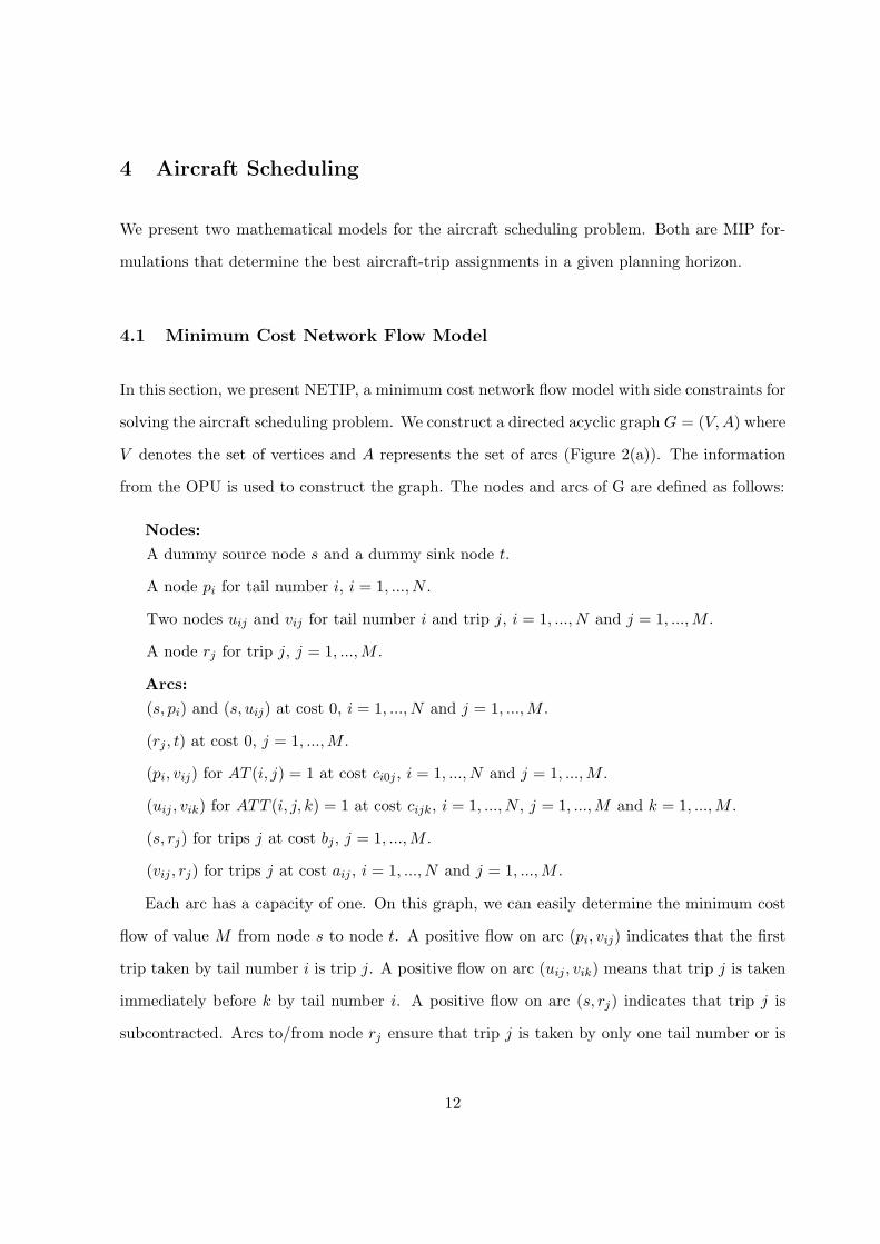
We present two mathematical models for the aircraft scheduling problem. Both are MIP for-

mulations that determine the best aircraft-trip assignments in a given planning horizon.

4.1 Minimum Cost Network Flow Model

In this section, we present NETIP, a minimum cost network flow model with side constraints for

solving the aircraft scheduling problem. We construct a directed acyclic graph G = (V,A) where

V denotes the set of vertices and A represents the set of arcs (Figure 2(a)). The information

from the OPU is used to construct the graph. The nodes and arcs of G are defined as follows:

Nodes:

A dummy source node s and a dummy sink node t.

A node pi for tail number i, i = 1, ..., N .

Two nodes uij and vij for tail number i and trip j, i = 1, ..., N and j = 1, ...,M .

A node rj for trip j, j = 1, ...,M .

Arcs:

(s, pi) and (s, uij) at cost 0, i = 1, ..., N and j = 1, ...,M .

(rj , t) at cost 0, j = 1, ...,M .

(pi, vij) for AT (i, j) = 1 at cost ci0j , i = 1, ..., N and j = 1, ...,M .

(uij , vik) for ATT (i, j, k) = 1 at cost cijk, i = 1, ..., N , j = 1, ...,M and k = 1, ...,M .

(s, rj) for trips j at cost bj , j = 1, ...,M .

(vij , rj) for trips j at cost aij , i = 1, ..., N and j = 1, ...,M .

Each arc has a capacity of one. On this graph, we can easily determine the minimum cost

flow of value M from node s to node t. A positive flow on arc (pi, vij) indicates that the first

trip taken by tail number i is trip j. A positive flow on arc (uij , vik) means that trip j is taken

immediately before k by tail number i. A positive flow on arc (s, rj) indicates that trip j is

subcontracted. Arcs to/from node rj ensure that trip j is taken by only one tail number or is

12

s

p1

t

r1

v11

u11

r3

p2

r2

v12

u12

v13

u13 v21

u21

v22

u22

v23

u23

(N=2)Aircraft

Feasible assignment

Outflow = 3

Chartered tripTrips(M=3)

Inflow = 3

1 2

2 3

1

2

1 2

3

1

2

Solution without side constraints:

Solution with side constraints:

Network Flow Graph A Possible Solution

(a) (b)

Figure 2: Illustration of the graph for the minimum cost network flow based formulation

subcontracted. Solving the minimum cost network flow problem on the given graph provides an

integer solution. Unfortunately, this solution does not correspond to a solution to the aircraft

scheduling problem unless side constraints are added. Consider the example shown in Figure 2

with 2 aircraft and 3 trips. Assume that the optimal solution to the minimum cost network flow

problem in Figure 2(a), is given by routes s → p1 → v11 → r1 → t, s → u11 → v12 → r2 → t

and s → u22 → v23 → r3 → t. Hence, all the trips are assigned to the aircraft. Interpreting

the solution in Figure 2(b), one sees that tail number 1 takes trip 1 as its first trip, followed

by trip 2. On the other hand, trip 3 is assigned to tail number 2. Although this is a feasible

schedule, it need not be optimal since the cost of the network flow solution is not the actual

cost of the schedule. In particular, the cost computation assumes that trip 2 precedes trip 3

(on tail number 2) but that is not the case. Therefore, such solutions need to be eliminated by

adding side constraints.

13

Side constraints are added to ensure that for each aircraft that serves trips j and k back-to-

back, trip j is either the first trip of that aircraft or it is preceded by another trip q. Unfortu-

nately, these side constraints destroy the total unimodularity of the constraint matrix, i.e., the

linear programming (LP) relaxation of the model is not guaranteed to have an integer solution.

Therefore, one has to work with a 0-1 integer programming formulation. Let x(e, f) to be the

flow from node e to node f on arc (e, f) of graph G. We provide the NETIP formulation below.

MinN∑

i=1

∑j:AT (i,j)=1

ci0j · x(pi, vij) +N∑

i=1

∑j:AT (i,j)=1

∑k:ATT (i,j,k)=1

cijk · x(uij , vik) (1)

+N∑

i=1

M∑j=1

aij · x(vij , rj) +M∑

j=1

bj · x(s, rj) (2)

s.t.N∑

i=1

x(s, pi) +M∑

j=1

x(s, rj) +N∑

i=1

M∑j=1

x(s, uij) = M (3)

M∑j=1

x(rj , t) = M (4)

x(s, pi)−∑

j:AT (i,j)=1x(pi, vij) = 0, i = 1, ..., N (5)

x(s, uij)−∑

k:ATT (i,j,k)=1x(uij , vik) = 0, ∀ i, j with AT (i, j) = 1 (6)

x(s, rj) +N∑

i=1

x(vij , rj)− x(rj , t) = 0, j = 1, ...,M (7)

x(pi, vik) +∑

j:ATT (i,j,k)=1x(uij , vik)− x(vik, rk) = 0,

k = 1, ...,M, ∀ i with AT (i, k) = 1 (8)

x(s, uij)− x(vij , rj) ≤ 0, i = 1, ..., N, j = 1, ...,M (9)

x(e, f) ∈ 0, 1, ∀ (e, f) ∈ A. (10)

The objective is to minimize total costs. The two terms in (1) are the repositioning costs,

whereas the first term in (2) represents the hidden costs of operation and the second one

represents the subcontracting cost. Constraints (3) - (8) ensure the flow balance of each node

14

in the network, and (9) are the side constraints. The side constraints ensure that there is no

flow from s to uij unless there is positive flow from vij to rj , i.e., trip j cannot precede another

trip on tail number i unless trip j is assigned to i.

Let ‖AT‖ and ‖ATT‖ denote the number of non-zero coefficients in the AT and ATT

matrixes respectively. NETIP has (N+2M+3‖AT‖+‖ATT‖) variables and (2+N+3M+‖AT‖)

constraints. The number of side constraints in (9) is NM , which increases with the fleet

size and the number of requested trips. The main advantages of NETIP are the ease of its

implementation using ILOG CPLEX and its underlying network structure. However, for large

fleet sizes and/or high load factors, side constraints dominate the network constraint matrix

and affect the solution time negatively. We present an alternative formulation to deal with this

issue.

4.2 Mixed Integer Programming Model

In this formulation (we call it MIPS) we use the following decision variables.

Sj =

1, if trip j is subcontracted

0, otherwise, j = 1, ...,M.

Zijk =

1, if tail number i serves trip j just before trip k

0, otherwise, ∀ i, j, k if ATT (i, j, k) = 1.

Zi00 =

1, if tail number i does not serve any trips

0, otherwise, i = 1, ..., N.

Zi0k =

1, if trip k is the first trip served by tail number i

0, otherwise, ∀ i, k if AT (i, k) = 1.

Zij0 =

1, if trip j is the last trip served by tail number i

0, otherwise, ∀ i, j if AT (i, j) = 1.

15

We provide the MIPS formulation below.

(MIPS) MinN∑

i=1

M∑j=1

ci0j · Zi0j +N∑

i=1

M∑j=1

M∑k=1

cijk · Zijk

+N∑

i=1

M∑j=1

M∑k=0

aij · Zijk +M∑

j=1

bj · Sj (11)

s.t. Sk +N∑

i=1

M∑j=0

Zijk = 1, k = 1, ...,M. (12)

M∑k=0

Zijk −M∑

q=0

Ziqj = 0, ∀i, j when AT (i, j) = 1. (13)

M∑k=0

Zi0k = 1, i = 1, ..., N. (14)

Zijk ∈ 0, 1, Sj ∈ 0, 1.

Similar to NETIP, the objective (equation (11)) is to minimize the total cost of repositioning

legs, hidden cost of operations, and subcontracting costs. Constraints (12) ensure that any

customer trip has to be served by a charter or by a company aircraft. Constraints (13) ensure

that if trip k is served right after trip j, then trip j is either the first trip of that tail number

or it is preceded by another trip q. Constraints (14) ensure that each tail number has a first

trip, or no trips at all. MIPS is related to the models presented in both [8] and [10]. MIPS

considers multiple types of aircraft and upgrade/downgrade, and hence generalizes the single

type aircraft model of [8]. However, as opposed to [8], MIPS does not consider maintenance

restrictions. On the other hand, the model in [10] considers scheduling multiple types of aircraft

subject to crew availability and MIPS is a special case of that model.

MIPS has (N +M +2‖AT‖+ ‖ATT‖) decision variables and (N +M + ‖AT‖) constraints,

significantly fewer than NETIP. Hence, it can potentially perform better especially in problems

with large fleet sizes and/or load factors.

16

Instance Load Factor (l) ‖AT‖ ‖ATT‖ Setup Time Solution Time(N,M) (M/N) NETIP MIPS NETIP MIPS

(40, 41) 1.02 519 294 0.02 0.03 0.05 0.02(44, 70) 1.59 1750 7330 0.19 0.58 1.16 0.42(51, 35) 0.69 977 1949 0.06 0.15 0.14 0.09(55, 71) 1.29 1354 2826 0.09 0.19 0.27 0.12(68, 135) 2.08 4295 23386 1.45 6.44 9.50 3.25(72, 62) 0.86 1564 4947 0.15 0.41 0.41 0.24(73, 90) 1.23 3056 12195 0.45 1.72 1.34 0.74(74, 49) 0.66 1441 3280 0.10 0.24 0.31 0.15(75, 105) 1.40 3764 19474 0.97 4.33 5.17 3.66(76, 100) 1.32 3683 11156 0.46 1.44 2.24 0.71

Table 1: Performance comparison of NETIP and MIPS on real data

4.3 Comparison of NETIP and MIPS

We have tested NETIP and MIPS using both real world and randomly generated data sets. The

results in Table 1 show the performance of the models on real data which was obtained during

the winter season of 2001. The load factors range from 0.66 to 2.08 for the given instances.

As we introduced in Sections 4.1 and 4.2 the number of decision variables and constraints

are functions of N, M, ‖AT‖ and ‖ATT‖. For instance, when (N,M) = (68, 135) there are

36,609 decision variables and 4,770 constraints in NETIP, and 32,179 decision variables and

4,498 constraints in MIPS. The column “Setup Time” denotes the time spent to retrieve the

preprocessed information and to prepare the formulations for CPLEX. The “Solution Time”

denotes the time for CPLEX solver to determine an optimal integer solution. The problems

are solved using ILOG CPLEX 7.5 on a PC with 1.13 GHz CPU and 512 MB memory, and

all computation times are reported in CPU seconds. The setup time of NETIP is shorter than

MIPS while NETIP requires longer solution time. The total computation time of NETIP (the

sum of setup time and solution time) during the trial period was no more than 12 seconds, and

in most cases less than 2 seconds, which is comparable to MIPS.

Although the results in Table 1 show that the run time of OE is satisfactory when either

NETIP or MIPS is used, this is not necessarily representative of the performance for future use.

17

With the expected growth of the fleet, the daily scheduling problems at the FMC will be of

significantly larger size. In addition, load factors can be as high as 2 to 3 during high seasons.

To examine the effect of fleet size and load factors on the computation time, we tested NETIP

and MIPS using randomly generated data sets.

The data is generated as follows: We first chose 100 cities that are uniformly distributed on

a 100 by 100 grid. The flight time between two adjacent points on the grid is assumed to be 3

minutes, therefore the longest flight is about 7 hours. Using the 100 cities, we randomly select

(i) the initial location of the aircraft and (ii) a departure location and destination location for

each trip with flight time greater than 30 minutes. The departure time for a trip is uniformly

distributed between 0 and 900 minutes. The earliest available time of each tail number is

uniformly selected between 0 and 600 minutes. There are 8 types of aircraft in the fleet and

an aircraft type is randomly selected for each trip. During the planning horizon a randomly

selected 20% of the fleet must go through maintenance services. Each maintenance service lasts

150 minutes. The data sets generated by this design mimic the FMC’s operations in a 24-hour

period.

We use five different fleet sizes N = 10, 30, 50, 70, 100 in our experiments. Each fleet size

is tested using load factors of 1, 2 and 3, yielding a total of 15 experiments. We generate 10

independent, random data sets for each experiment. We report the average performance with

respect to each experiment in Table 2.

The last two columns in Table 2 show the average number of nodes accessed by the branch-

and-bound (B&B) scheme used in ILOG CPLEX. Because of its special structure, NETIP

needs smaller number of nodes in a B&B tree in most cases. In 91% of the random data sets

tested, the LP relaxation of at least one of the formulations solves the problem optimally (i.e.,

zero B&B nodes). Among those data sets, there are a few cases where the LP relaxation of

MIPS yields the integer solution while NETIP fails to do so, and vice versa. We infer from our

experiments that neither formulation is tighter than the other.

The solution time varies dramatically with fleet size and load factor. With small fleet sizes

18

Experiment Load ‖AT‖ ‖ATT‖ Setup Time Solution Time B&B Nodes(N, M) Factor (l) NETIP MIPS NETIP MIPS NETIP MIPS(10, 10) 1 43 20 0.01 0.01 0.01 0.01 0 0(10, 20) 2 85 91 0.01 0.01 0.01 0.01 0 0(10, 30) 3 133 195 0.01 0.02 0.02 0.01 0 0(30, 30) 1 382 549 0.02 0.05 0.04 0.02 0 0(30, 60) 2 741 2013 0.04 0.16 0.17 0.09 0 0(30, 90) 3 1110 4315 0.08 0.36 0.95 0.34 0 0(50, 50) 1 1006 2117 0.05 0.18 0.17 0.11 0 0(50, 100) 2 2061 9093 0.22 1.17 2.93 1.08 1 1(50, 150) 3 3121 21128 0.71 4.05 31.95 8.42 2 5(70, 70) 1 2036 6181 0.17 0.71 0.59 0.35 0 0(70, 140) 2 4074 25429 1.17 5.89 29.54 8.70 4 4(70, 210) 3 6115 56023 4.07 18.82 246.21 55.28 27 14(100, 100) 1 4091 18560 0.90 4.07 2.56 1.75 0 0(100, 200) 2 8146 70823 6.82 28.79 212.07 46.48 12 2(100, 300) 3 12274 164320 28.22 101.79 2154.82 868.58 64 177

Table 2: Performance comparison between NETIP and MIPS on randomly generated data

and low load factors, NETIP is slightly faster than MIPS. When fleet size and load factor

increase, MIPS has a significantly faster solution time, and a better total computation time

overall even though its setup time is higher than NETIP. For example, when N = 100 and

M = 300, it takes around 16 minutes for MIPS to generate the optimal solution compared to

36 minutes by NETIP. Therefore, MIPS could be a better choice than NETIP for the FMC in

the future since the fleet size is expected to increase further.

5 Combined Aircraft and Crew Scheduling

Under FAA regulations the duty period of a crew cannot exceed more than 14 hours (we call it

DUTY ). Each duty period must be followed by a rest period of at least 10 consecutive hours.

The start time of a duty period is defined as when a crew serves its first flight of the day (which

can be a customer trip, or a repositioning flight), rather than the time a crew ends its previous

rest period and becomes ready for service. Therefore, while creating a schedule, only those trips

that can be served within DUTY hours since the first flight departure of an aircraft are eligible

19

to be assigned to that aircraft. This restriction can be easily handled at the preprocessing stage

if the duty start time of each crew is known. For instance, if a tail number starts its duty at 9

a.m. and DUTY = 14 hours, the information in matrix AT can be updated easily to make sure

that the tail number does not take any trips that require flying past 11 p.m. Unfortunately, the

only information that is available prior to creating a schedule is when the crew first becomes

available for service. The actual duty start time of a crew-aircraft pair depends on the first trip

assigned to that aircraft.

In this section, we present a heuristic and two exact models to solve the scheduling problem

when aircraft are subject to crew availability. First we present a heuristic based on the idea

that MIPS (or NETIP) solutions can be “corrected” in a simple manner. The first mathe-

matical model enhances MIPS by adding explicit constraints on crew duty time. The second

model is a set partitioning formulation. These enhanced approaches fit the architecture of the

FlightOptimizer and can easily be incorporated into the OE.

5.1 A Heuristic Based on Simple Correction to MIPS

The heuristic is based on the idea that the solution to MIPS (or NETIP) will more likely be

feasible for the combined aircraft and crew scheduling problem, if the crew availability can be

appropriately preprocessed in the OPU. Suppose there is a service period of DUTY hours for

each aircraft. This spans the period when the crew is “available”, i.e., it includes the duty time

as well as the idle time before duty, when the crew is available but not used for service. Matrix

AT can be updated accordingly: Starting from the earliest time a tail number is available, it

will remain in service for the next DUTY hours, and cannot take any trips that require flying

beyond this duty period. The main advantage of this heuristic is that it is easily incorporated

into NETIP and MIPS without affecting the computation times to create a Master Schedule.

The disadvantage is that the schedule obtained may violate the actual crew duty time limits or

impose tighter than necessary duty constraints on the aircraft. Choosing a conservative value

for DUTY , say DUTY = 14 hours, will ensure schedule feasibility, but possibly lead to lower

20

aircraft utilization and higher cost. On the other hand, longer DUTY results in a more cost-

efficient schedule, but at a higher risk of infeasibility. We tested different DUTY from 14 to 16

hours with increments of half an hour. Our computational results indicate that DUTY = 14.5

hours achieve the best tradeoff between schedule feasibility and schedule efficiency in terms of

total operational cost.

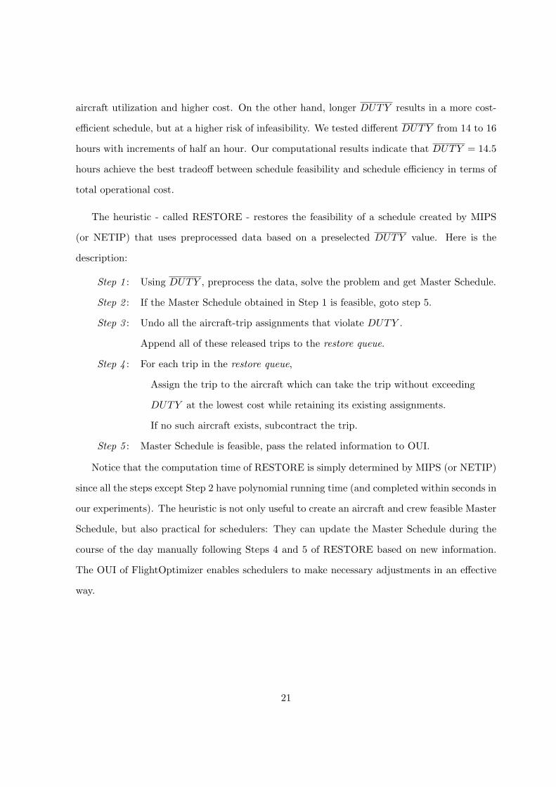
The heuristic - called RESTORE - restores the feasibility of a schedule created by MIPS

(or NETIP) that uses preprocessed data based on a preselected DUTY value. Here is the

description:

Step 1 : Using DUTY , preprocess the data, solve the problem and get Master Schedule.

Step 2 : If the Master Schedule obtained in Step 1 is feasible, goto step 5.

Step 3 : Undo all the aircraft-trip assignments that violate DUTY .

Append all of these released trips to the restore queue.

Step 4 : For each trip in the restore queue,

Assign the trip to the aircraft which can take the trip without exceeding

DUTY at the lowest cost while retaining its existing assignments.

If no such aircraft exists, subcontract the trip.

Step 5 : Master Schedule is feasible, pass the related information to OUI.

Notice that the computation time of RESTORE is simply determined by MIPS (or NETIP)

since all the steps except Step 2 have polynomial running time (and completed within seconds in

our experiments). The heuristic is not only useful to create an aircraft and crew feasible Master

Schedule, but also practical for schedulers: They can update the Master Schedule during the

course of the day manually following Steps 4 and 5 of RESTORE based on new information.

The OUI of FlightOptimizer enables schedulers to make necessary adjustments in an effective

way.

21

5.2 A MIP Model With Hard Constraints on Crew Duty Times

In a 24-hour planning horizon, there is only one duty period for the crew followed by a rest

period. Let stime(j) be the departure time of trip j, ttime(i, k) be the total travel time for

aircraft i taking trip k and atrepo(i, j) be the repositioning time from the location of aircraft i

to the departure of trip j. The constraints

∑k:AT (i,k)=1

[stime(k) + ttime(i, k)] · Zik0

−∑

j:AT (i,j)=1[stime(j)− atrepo(i, j)] · Zi0j ≤ DUTY (15)

are added to MIPS for each i = 1, ..., N to ensure that the time between the first departure

of the day (i.e., the time aircraft starts service) and the last landing of the day (i.e., the time

aircraft completes service) does not exceed DUTY hours. We call this new MIP formulation

MIPS-CREW.

5.3 A Set Partitioning Based Formulation

An alternative approach for solving the aircraft scheduling problem with crew duty time re-

strictions is to use a set partitioning formulation. The idea is to assign tail numbers to feasible

routes to ensure that each tail number is assigned to at most one route and each trip is assigned

to a tail number or a charter. The set partitioning approach is very appealing for problems

where costs are nonlinear and discrete, and complicated operational rules are imposed. One

such problem is crew scheduling by commercial airlines [2], which is similar to the combined

aircraft and crew scheduling problem faced by FMCs. In both cases, “resources” (aircraft in

case of FMCs and crew in case of commercial airlines) have to be assigned to a set of trips, and

all trips have to be covered. However, there are three major differences: (i) Each crew schedule

in commercial airlines starts and ends at the same crew base, which is the city where the crew

is stationed. In FMCs, even though the crew travel to their home bases periodically, they can

22

come on or off duty at any location because of the nature of the business. The travel from a

home base to the location where the duty is to start is usually provided by means other than

the company aircraft. (ii) Commercial airlines aim to minimize the costs related to long or

frequent layovers within a duty period, long overnight rests away from base, and repositioning.

FMCs minimize the repositioning cost, subcontracting cost and hidden costs. The repositioning

is rare in commercial airlines while it is common in FMCs. (iii) Subcontracting is not an option

in commercial airlines.

We use the following notation in our formulation:

Ωi = the set of feasible routes for tail number i, i = 1, ...,M + N .

p = a feasible route, p ∈ Ωi.

cip = the total cost of taking route p by tail number i, i = 1, ...,M + N and p ∈ Ωi.

aijp =

1, if trip j is on route p

0, otherwise, p ∈ Ωi, i = 1, ...,M + N and j = 1, ...,M .

θip =

1, if tail number i takes route p

0, otherwise, p ∈ Ωi and i = 1, ...,M + N .

Note the tail numbers are indexed from 1 to N + M where the last M tail numbers denote

charters as opposed to company aircraft. Each tail number N + i has only one feasible route

which is associated with trip i, and the cost of the route is the charter cost of that trip. Feasible

routes for the company aircraft can be determined using the same preprocessing rules used by

MIPS (see Section 3.1) ensuring that the crew duty limits are not exceeded when a number of

trips are assigned to an aircraft.

The Master Problem (MP) is

(MP ) MinM+N∑i=1

∑p∈Ωi

cipθip

M+N∑i=1

∑p∈Ωi

aijpθip = 1, j = 1, ...,M (16)

23

∑p∈Ωi

θip ≤ 1, i = 1, ...,M + N (17)

θip ∈ 0, 1, i = 1, ...,M + N, and p ∈ Ωi. (18)

where constraints (16) ensure that each trip is taken either by one tail number or by a charter

and constraints (17) ensure that a tail number is assigned to at most one route.

One possible approach (we call it SP) for solving MP is to generate all feasible routes and

then solve the model as a standard integer program. There are two drawbacks of this approach.

The number of feasible routes might be quite high, hence, generating all of them may not be

computationally feasible. Even if the routes could be generated, the resulting model might

not be solvable in a reasonable time with a commercial solver, given the high number of 0-1

variables. Given these drawbacks of SP, the author of [12] follows a slightly different approach

for solving the set partitioning model for charter aircraft scheduling problem. He generates only

a subset of the feasible routes, and then uses a customized solver. While it is computationally

more efficient than SP, this approach does not guarantee optimality. Another approach for

solving the (large scale) set partitioning problems is branch-and-price (BP), which combines

column generation and branch-and-bound (B&B). Next, we discuss the BP approach we used

for solving the combined aircraft and crew scheduling problem.

5.3.1 Branch and Price Method

The standard approach to solving integer programming problems is branch-and-bound (B&B).

At each branch of the B&B tree, we solve the LP relaxation of the integer problem. However,

given the large number of potential columns (variables) in the MP, generating all columns

upfront and solving the relaxation of MP exactly might be challenging. A computationally more

efficient approach is column generation. The general idea of column generation is to start with

a manageable subset of columns and generate new favorable columns to enter the basis. The

linear relaxation of MP over a subset of the variables is called the restricted master problem

24

(RMP). The BP method first solves the RMP for a given set of columns using the simplex

method. Then, dual variables αj and γi where i = 1, ...,M + N and j = 1, ...,M , associated

with constraints (16) and (17) respectively, are generated and passed to the following pricing

subproblem - called PP -

(PP ) Minp∈Ωi cip = cip −∑j

αjaijp − γi, i = 1, ..., N + M, (19)

to price out favorable columns. Let cip be the updated marginal cost for tail number i taking

route p. If cip ≥ 0 for all i = 1, ..., N + M , then there is no column with a negative reduced

cost and the current primal solution solves the RMP optimally. Otherwise, a subset of new

columns is selected and added to the RMP. This completes one iteration and the enlarged RMP

is re-optimized. The procedure continues until no column with negative reduced cost can be

found.

These ideas are combined with a B&B scheme in the following branch-and-price algorithm.

Step 1 : Determine an initial set of feasible columns, form the RMP, and go to Step 3.

Step 2 : Choose a variable (or node) to branch.

Step 3 : Solve the LP relaxation of the RMP and pass the dual variables to the PP.

Step 4 : If columns with negative reduced costs in the PP exist,

select a subset of those columns, add them to the RMP and go to Step 3.

Otherwise, go to Step 5.

Step 5 : If solution is integral, fathom. Otherwise, go to Step 2.

Branch-and-price approach has been used to solve large integer programs. For more infor-

mation about this approach and implementation issues see [16] and [14].

5.3.2 Implementing the Branch and Price Algorithm

In this section we discuss several important implementation issues involved in the BP.

25

Feasible Routes: The pricing problem is to select favorable feasible routes and add them

to the RMP. Filtering the input data via the OPU eases the creation of feasible routes. To

generate a feasible route for tail number i, we can simply start with its first trip, say j1 if

AT (i, j1) = 1. Its second trip j2 can be appended to the route if ATT (i, j1, j2) = 1, a third trip

j3 is appended if ATT (i, j2, j3) = 1 and so on. This procedure continues as long as crew duty

time restrictions for an aircraft are not violated.

Pricing Strategy: We need to decide which of the favorable columns to price out from the

PP to incorporate into the RMP. Detailed discussions are provided in [1] and [17] on selecting

favorable columns. Their computational experience suggests that if the pricing problem can

be solved to optimality in an efficient manner, then adding only the most profitable column

is the best strategy. The pricing subproblem in our application (the combined aircraft and

crew scheduling problem), i.e., generating the most profitable feasible column, is a constrained

shortest path problem, which is NP-complete. To solve the pricing subproblems exactly, we

generate all feasible routes once at the very beginning (using the filtered input data from

the OPU in the FlightOptimizer), and then select the most profitable feasible route at each

node of the branch-and-bound tree (and at each iteration of column generation) by complete

enumeration. For large problem instances, our computational results show that the BP approach

implemented in this fashion is more efficient than SP. Note that since we solve the pricing

subproblem exactly, our implementation of BP is an exact solution approach.

Branching Rule: Since the coefficients of the constraint matrix in our problem are all binary,

we use the branching idea introduced by [13], which leads to a general branching rule where

rows l and m should be covered by the same column on one branch and by different columns on

the other. Applied to our problem, it simply requires that trips l and m be covered by the same

feasible route on the left branch and by different feasible routes on the right branch. Columns

in the RMP violating the branching constraints are removed and only the columns satisfying

the branching constraints are priced out from the PP. Since the number of branching pairs is

finite, the algorithm terminates after a finite number of branches. When no more branching

26

0.00%

0.20%

0.40%

0.60%

0.80%

1.00%

1.20%

(50, 100) (50, 150) (70, 140) (70, 210) (100, 200) (100, 300)

Experiments

Co

st S

avin

g O

ver

RE

ST

OR

E

Average Maximum

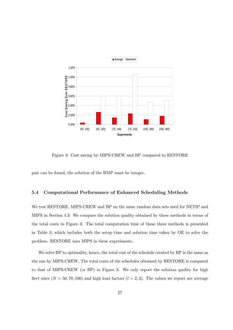
Figure 3: Cost saving by MIPS-CREW and BP compared to RESTORE

pair can be found, the solution of the RMP must be integer.

5.4 Computational Performance of Enhanced Scheduling Methods

We test RESTORE, MIPS-CREW and BP on the same random data sets used for NETIP and

MIPS in Section 4.3. We compare the solution quality obtained by these methods in terms of

the total costs in Figure 3. The total computation time of these three methods is presented

in Table 3, which includes both the setup time and solution time taken by OE to solve the

problem. RESTORE uses MIPS in these experiments.

We solve BP to optimality, hence, the total cost of the schedule created by BP is the same as

the one by MIPS-CREW. The total costs of the schedules obtained by RESTORE is compared

to that of MIPS-CREW (or BP) in Figure 3. We only report the solution quality for high

fleet sizes (N = 50, 70, 100) and high load factors (l = 2, 3). The values we report are average

27

Experiment Total Computation Time(N,M) RESTORE MIPS-CREW BP

(10, 10) 0.01 0.01 0.61(10, 20) 0.02 0.02 0.64(10, 30) 0.03 0.05 0.65(30, 30) 0.07 0.17 0.77(30, 60) 0.26 0.97 1.40(30, 90) 0.70 4.14 2.92(50, 50) 0.30 1.86 1.61(50, 100) 2.25 13.47 8.88(50, 150) 12.47 77.12 27.27(70, 70) 1.06 2.53 6.02(70, 140) 14.58 63.09 47.21(70, 210) 74.10 744.69 158.26(100, 100) 5.82 21.87 28.17(100, 200) 75.27 357.65 259.56(100, 300) 970.38 12709.20 1359.12

Table 3: Average computation time of RESTORE, MIPS-CREW and BP to solve randomlygenerated problems

and maximum values over all the ten instances randomly created in each experiment. The cost

savings (in percentage) achieved by MIPS-CREW and BP over RESTORE are represented in

Figure 3. RESTORE can obtain feasible schedules that have costs 0.27% (on average) higher

than the optimal solution. The maximum optimality gap for RESTORE is less than 1.1%.

MIPS-CREW generates optimal solutions at a cost of long computation time. MIPS-CREW

outperforms BP in small size problems. However, when N ≥ 50 and l ≥ 2, BP’s computational

advantage becomes visible. When (N,M) = (100, 300), it takes around 22 minutes for BP to

generate an optimal solution, which is nine times faster than MIPS-CREW. RESTORE is faster

than both MIPS-CREW and BP.

In general, although MIPS-CREW creates optimal schedules, it is too slow to be a practical

solution. RESTORE is a promising alternative for practical purposes in terms of simplicity,

solution quality and computation time. However, it is not flexible to handle longer planning

horizons with multiple duty periods. BP is potentially the best alternative for solving large

scale problems with high load factors and long planning horizons.

28

Aircraft Scheduling Combined Aircraft and Crew Scheduling

NETIP MIPS RESTORE MIPS-CREW BPComplexity in

Implementation Low Medium Medium Medium HighOptimality

Solution Quality Optimal Optimal gap range Optimal Optimal(0, 0.27%)

Flexibility Low Low Low Low HighAverage SL (0.02, 0.22) (0.02, 0.29) (0.02, 0.29) (0.01, 1.86) (0.61, 1.61)

Computation SH (0.02, 32.66) (0.02, 12.47) (0.02, 12.47) (0.02, 77.12) (0.64, 27.27)Time LL (0.22, 3.46) (0.29, 5.83) (0.29, 5.83) (1.86, 21.87) (1.61, 28.17)

(CPU seconds) LH (3.15, 2183) (2.25, 970) (2.25, 970) (13.47, 12709) (8.88, 1359)

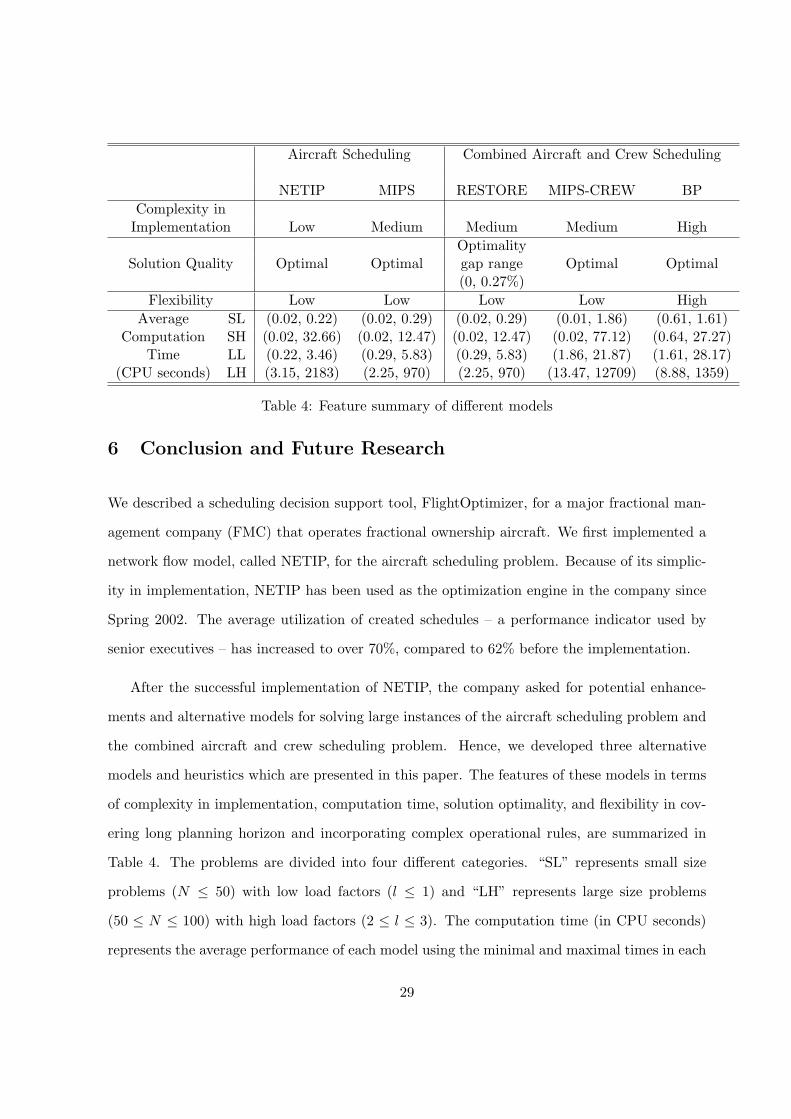
Table 4: Feature summary of different models

6 Conclusion and Future Research

We described a scheduling decision support tool, FlightOptimizer, for a major fractional man-

agement company (FMC) that operates fractional ownership aircraft. We first implemented a

network flow model, called NETIP, for the aircraft scheduling problem. Because of its simplic-

ity in implementation, NETIP has been used as the optimization engine in the company since

Spring 2002. The average utilization of created schedules – a performance indicator used by

senior executives – has increased to over 70%, compared to 62% before the implementation.

After the successful implementation of NETIP, the company asked for potential enhance-

ments and alternative models for solving large instances of the aircraft scheduling problem and

the combined aircraft and crew scheduling problem. Hence, we developed three alternative

models and heuristics which are presented in this paper. The features of these models in terms

of complexity in implementation, computation time, solution optimality, and flexibility in cov-

ering long planning horizon and incorporating complex operational rules, are summarized in

Table 4. The problems are divided into four different categories. “SL” represents small size

problems (N ≤ 50) with low load factors (l ≤ 1) and “LH” represents large size problems

(50 ≤ N ≤ 100) with high load factors (2 ≤ l ≤ 3). The computation time (in CPU seconds)

represents the average performance of each model using the minimal and maximal times in each

29

category.

For the aircraft scheduling problem, MIPS works better than NETIP, especially for the

problems in the “LH” category. Among the solutions for the combined aircraft and crew

scheduling problem, MIPS-CREW provides optimal solutions (for a 24-hour horizon) but is too

slow to be practical. On the other hand, RESTORE can generate schedules quickly with an

average optimality gap of 0.27%. Thus, RESTORE is a preferred quick add-on solution for a 24-

hour planning horizon. However, to solve large size problems covering longer planning horizons

and to incorporate complicated operational rules, we believe that BP is a better alternative.

With our flexible, module-based decision support tool, alternative optimization models can be

easily plugged into FlightOptimizer to accommodate different operational requirements.

Several extensions to our model are under investigation to address other practical challenges

faced by the FMC: (i) In fractional ownership programs both demand and aircraft supply change

dynamically over time. For instance in the FMC around 25% of the requested trips arrive after

the original schedule is created, and each day 10-12 aircraft require unplanned maintenance.

Current schedule optimization is done by assuming that the demand and supply information

is deterministic over the planning horizon. When there is a change on either side, the schedule

has to be modified, but has to remain close to the original one because of several practical

factors. A common complaint from managers when using optimization-based decision support

tools is that small changes in input often translate into dramatically different solutions that

sometimes are not managerially acceptable [3]. Therefore we aim to enhance FlightOptimizer

so that it can update the schedule to accommodate disruptions in real time while keeping it as

close to the original one as possible. (ii) All the models presented here are tested numerically

for a 24-hour planning horizon. RESTORE cannot be adjusted in a straightforward way to

solve problems with longer planning horizons that involve multiple duty periods. Alternative

models are presented in [6] for multiple day horizons. However, they are MIP models and likely

to have poor computation time with general purpose solvers. BP remains a promising solution

with only minor complications in determining feasible routes. (iii) Current scheduling solutions

30

consider all the trip requests as firm demand that must be satisfied by company aircraft or

charter aircraft. However, it is possible that some demand is optional, i.e., should be satisfied

only if it is profitable. The FMC currently sees at least two sources of optional demand: Charter

requests from other companies and special requests from customers in excess of their available

flight hours. We believe that enhancing the current models to incorporate optional demands is

an interesting and challenging extension.

References

[1] C. Barnhart, E.L. Johnson, G.L. Nemhauser, M.W.P. Savelsbergh, and P.H. Vance.

Branch-and-price: Column generation for solving huge integer programs. Operations Re-

search, 46(3):316–329, 1998.

[2] C. Barnhart, E.L. Johnson, G.L. Nemhauser, and P.H. Vance. Crew scheduling. In R.W.

Hall, editor, Handbook of Transportation Science, pages 493–521. Kluwer Scientific Pub-

lishers, 1999.

[3] G. Brown, R. Dell, and R. Wood. Optimization and persistence. Interfaces, 27(5):15–37,

1997.

[4] S. Carey. Ultimate upgrade: More fliers decide that 1st class just isn’t good enough. The

Wall Street Journal, page 1, April 23 2002.

[5] E. David. Outlook: Fractional ownership. Business& Commercial Aviation, 91(2):66,

August 2002.

[6] I. Karaesmen and P. Keskinocak. A note on scheduling time-shared aircraft: Alterna-

tive formulations for scheduling the aircraft subject to crew availability. Working paper,

University of Maryland, College Park, MD, 2003.

[7] P. Keskinocak. Corporate high flyers. OR/MS Today, December 1999.

31

[8] P. Keskinocak and S. Tayur. Scheduling of time-shared jet aircraft. Transportation Science,

32(3):277–294, 1998.

[9] J.L. Levere. Buying a share of a private jet. The New York Times, 1996.

[10] C. Martin, D. Jones, and P. Keskinocak. Optimizing on-demand aircraft schedules for

fractional aircraft operators. Interfaces, 33(3):22–35, September-October 2003.

[11] National Business Aviation Association, Washington DC. NBAA Business Aviation Fact-

book, 2002.

[12] D. Ronen. Scheduling charter aircraft. Journal of Operational Research Society, 51:258–

262, 2000.

[13] D.M. Ryan and B.A. Foster. An integer programming approach to scheduling. In

A. Wren, editor, Computer Scheduling of Public Transport Urban Passenger Vehicle and

Crew Scheduling, pages 269–280. North-Holland, 1981.

[14] M.W.P. Savelsbergh. A branch-and-price algorithm for the generalized assignment prob-

lem. Operations Research, 45(6):831–841, 1997.

[15] P. Sheridan. Some advantages of private aviation. Pittsburgh Post Gazette, January 21

2002.

[16] P.H. Vance, C. Barnhart, E.L. Johnson, and G.L. Nemhauser. Airline crew scheduling: A

new formulation and decomposition algorithm. Operations Research, 45(3):183–200, 1998.

[17] F. Vanderbeck. Decomposition and column generation for integer programs. Technical

report, Universite Catholique de Louvain, Belgium, 1994.

[18] A.L. Velocci, Jr. Fractional ownership programs finding new software essential. Aviation

Week & Space Technology, June 1 2002.

[19] A. Zagorin. Rent-a-jet cachet. Time Magazine, September 13 1999.

32