Technical Memorandum No. 26

PRODUCTION AUTOMATION PROJECT College of Engineering & Applied Science The University of Rochester Rochester, New York

14627

TM-26

BOOLEAN OPERATIONS IN SOLID MODELLING: BOUNDARY EVALUATION AND MERGING ALGORITHMS

by

Aristides A. G. Requicha Herbert B. Voelcker

January 1984

The work described in this document was supported primarily by the National Science Foundation under Grants ECS-8104646 and MEA-8211424, and by companies in the Production Automation Project's Industrial Associates Program. Any opinions, findings, conclusions or recommendations expressed in this publication are those of the authors and do not necessarily reflect the views of the National Science Foundation or the Industrial Associates of the P.A.P. An earlier version of this paper was presented orally in an Advanced Topics Seminar on Solid Modelling at SIGGRAPH '83, Detroit, MI, July 1983.

ABSTRACT Solid modelling plays a key role in electromechanical CAD/CAM

(Computer Aided Design and Manufacture), three-dimensional computer graphics, computer vision, robotics, and other disciplines and activities that deal with spatial phenomena. All of the twenty-or-so solid modellers currently available in the U.S. support Boolean operations akin to set intersection, union and difference on solid objects. Boundary representations, i.e., face/edge/vertex structures, for solids defined through Boolean operations are generated in these modellers by using so-

called boundary evaluation and merging procedures. These are the most complex and delicate software modules in a solid modeller.

This paper describes boundary evaluation algorithms used by the PADL solid modelling systems developed at the University of Rochester, and discusses other known approaches in terms of the concepts of set membership classification and neighborhood manipulation, which emerged from the PADL work.

TABLE OF CONTENTS

1. Introduction . . . . . . . . . . . . . . . . . . . . . . . 1 1.1 Solid Modelling . . . . . . . . . . . . . . . . . . . . 1 1.2 Boolean Operations . . . . . . . . . . . . . . . . 1 1.3 The Computational Problems . . . . . . . . . . . . . . 5 1.4 Goals and Organization of the Paper . . . . . . . . . . . . 8

2. Set Membership Classification . . . . . . . . . . . . . . . . 10

2.1 Definitions . . . . . . . . . . . . . . . . . . . . 10 2.2 Combining Classifications . . . . . . . . . . 11 2.3 Representing and Combining Neighborhoods . . . 16 2.4 The Divide-and-Conquer Paradigm for Classification on CSG . . 23 2.5 Classification Algorithms for BReps . . . . . . . . . . . . 25

3. Boundary Evaluation and Merging . . . . . . . . . . . . . 34

3.1 The Generate-and-Test Paradigm for Faces . . . . . . . . 34 3.2 The Generate-and-Test Paradigm for Edges . . . . . . . 36 3.3 Efficiency Improvements . . . . . . . . . . . . . . . 44 3.4 Brief Survey of Known Approaches . . . . . . . . . 48 3.5 Topics Not Addressed in This Paper . . . . . . . . . 48

4. Summary and Concluding Remarks . . . . . . . . . . . . 50

5. Acknowledgements and Historical Notes . . . . . . . . . . 51

References . . . . . . . . . . . . . . . 531. Introduction

1.1 Solid Modelling Geometric modelling is concerned with (1) computational representations

for geometric entities (solids, surfaces,...) and transformations (rigid motions, Boolean operations,...), (2) algorithms for geometric reasoning, and for computing geometric properties and the effects of transformations, (3) mathematical theories that underlie such representations and algorithms, and (4) hardware and software systems in which they are imbedded. Geometric modelling plays a key role in electromechanical computer-aided (or automatic) design and production, computer graphics, computer vision, robotics, and other disciplines and activities that deal with spatial phenomena.

Solid modelling encompasses an emerging body of theory, techniques and systems centered on "informationally complete" representations of solids --representations that permit (at least in principle) any well-defined geometric property of any represented solid to be calculated automatically. Research in solid modelling has been underway at academic and industrial laboratories throughout the industrialized world for more than a decade, and solid modelling technology reached the marketplace and entered industrial use recently. Some twenty solid modelling systems are commercially available in the U.S., and their number is growing rapidly. The technology is eliciting great interest because it promises to provide the tools for automating such tasks as drafting, mesh generation for finite element analysis, and verification of programs for computer-controlled machine tools and manipulators. These tasks traditionally were performed manually or through computer-aided systems that required much user interaction because they were based on incomplete geometric models. (The history of solid modelling is summarized in [Requicha and Voelcker 19821, which also contains a slightly obsolescent view of the field; an up-to-date assessment of its current status, and a survey of current western-world research may be found in [Requicha and Voelcker 19831.)

1.2 Boolean Operations: Virtually all the available solid modellers provide some form of support for

Boolean operations (akin to set-theoretic union, intersection and difference) on solid objects. Boolean operations are used in solid modelling in at least thefollowing three contexts. To define solid objects through "additions" and "subtractions" of parameterized solid primitives such as cuboids and cylinders (Figure 1). To model and simulate manufacturing processes such as milling and drilling (Figure 2). To detect spatial interferences and collisions (Figure 3).

Successive stages in the definition of a mechanical part in the PADL-1 modelling system by using Boolean operations.

Agure t

A straight-line milling operation can be modelled and simulated by subtracting the region of space swept by the cylindrical cutter from the initial workpiece.

Agure 8 The assembly shown in (a) is not physically realizable because the intersection of the rotor and the bracket is non-null, as shown by the solid lines in (b). It is essential that solids be algebraically closed under Boolean operations to

3 ensure that results can be used as inputs for further operations, and that (models of) physical manufacturing processes produce valid solids [Tilove and Requicha 1980]. The standard set operators do not preserve solidity and therefore must be replaced by their regularized versions to ensure closure - see Figure 4. The theory of so-called r-sets. (for modelling solids) and regularized set operators is well understood, and can be found in [Requicha 1977, Requicha and Tilove 1978,

Requicha 19801. For the purposes of this paper an intuitive understanding of the basic concepts is sufficient. R--sets can be viewed as "curved polyhedra" without "dangling" edges or faces. When applied to solids (r-sets) regularized union (0) coincides with standard union. The regularized difference ( *) ensures that a solid 5 = A ---.#B includes all of its boundary, portions of which may be missing in the standard difference A - B. Regularized intersection ((f) differs from its standard counterpart only when solids have overlapping boundaries. Regularized intersection may involve discarding extraneous ("dangling") faces and edges contained in the standard intersection Aft B, as shown in Figure 4. (Technically, an r--set is a topologically closed, regular, semi analytic subset of three-dimensional Euclidean space. Regularized intersection is defined as Af PB = ki(A n B), where k and ti denote, respectively, topological closure and interior; the other regularized operators are defined similarly. R-sets and regularized set operators form a Boolean algebra.)

E

Agure 4 The standard set theoretical intersection of the cuboid B and the L-shaped solid A (a) is not a solid

because it has "dangling faces" (b), and therefore must be regularized as shown in (c).

14 The Computations) Problems There are many computational versions of what one can call "the

mathematical problem of evaluating regularized set operations on solids". These versions differ primarily in the representations that are assumed for the input and output solids. For example, if the input and output solids are represented by octrees, Boolean operations can be performed by known and relatively straightforward algorithms [Meagher 1982]. We are concerned in this paper only with boundary representations (abbreviated BReps) and CSG (Constructive Solid Geometry) representations [Requicha 19801 - see Figure 5. CSG representations are trees whose internal nodes represent Boolean (i.e., regularized set) operators or rigid motions, and whose leaves represent instances of parameterized primitive solids, e.g., variably-sized and positioned cuboids and cylinders. (For simplicity

5 of exposition rigid motions are ignored in this paper, but they are easy to accommodate in the algorithms to be presented.) BReps are graphs whose nodes represent faces, edges and vertices, and whose links represent incidence and adjacency relations.

SOLM

FAI)

A COG -REPRESENTATION A BOUNDARY REPRESENTATION

Fiipure 5 A simple solid, and its associated CSG tree and BRep.

Specifically, the problems to be addressed in this paper are the following. (The problem designations are Rochester jargon; no universally accepted designations exist.) • Non-incremental boundary evaluation: Given a CSG representation for a solid

S, And a BRep for S. • Boundary merging: Given BReps for two solids A and B find a BRep for S =

A ® B, where ® denotes one of the regularized operators. • Incremental boundary evaluation: Given BReps and CSG representations for A

and B, find a BRep for S. (A CSG representation for S can be 6

generated trivially.) Boundary evaluation and merging procedures (called in Rochester jargon

boundary evaluators) are probably the most complex and delicate software modules in solid modelling systems. To understand the role of boundary evaluators, consider the two basic architectures used by current solid modellers and shown in Figure 6. Users of single-representation systems based on BReps (Figure 6a) define objects through Boolean operations on previously defined objects, and also by direct boundary manipulation and other means. CSG trees are not maintained by these systems - and indeed cannot be constructed for objects whose definitions include non-Boolean operations - and therefore boundary merging algorithms must be invoked to convert the user definitional data into internal BReps.

ARLIdQIOU ws WUMICS ~ssroors

ro WLIuria ws

Agure 6

Two basic architectures for solid modellers. Dual-representation systems (Figure 6b) derive BReps from CSG. Conversion

of CSG into a BRep can be accomplished by non-incremental boundary evaluation, or by either boundary merging or incremental boundary evaluation procedures used recursively. Non-incremental operation can be useful, for example when stored "library" objects are brought into a user's "workspace". (Modified non-incremental evaluators can also be used profitably for interference detection and related

7 problems [Tilove 1984].) However, human users of solid modellers normally interact with the systems by constructing objects progressively, typically by successively unioning and differencing primitives or library objects from a current object. BRep updating in this context can be accomplished most efficiently by boundary merging or incremental boundary evaluation procedures, which operate incrementally and use boundary information computed for previously defined objects. User feedback is provided in almost all solid modellers through calligraphic (line) displays, which are generated from BReps. Reasonable response times can only be achieved if BReps are updated rapidly, and therefore incremental algorithms (either for boundary merging or incremental boundary evaluation) must be used. (This' situation may change when VLSI chips for generating displays directly from CSG become available [Kedem and Ellis 19841.)

1.4 Goals and Organization of the Paper Almost all solid modellers support Boolean operations, as noted earlier, but

very few descriptions of the algorithms used are available, and these have appeared mainly in internal reports of limited circulation. <'>

In particular, the boundary evaluation algorithms used by the PADL-1 [Voelcker et al. 1978] and PADL-2 [Brown 1982] systems developed at the University of Rochester have never been published, although they were designed in the mid 1970's.

The main goals of this paper are (1) to describe a family of algorithms used for boundary evaluation in the PADL systems and (2) to use the concepts of set membership classification and neighborhood manipulation, which arose from the PADL work, to describe other approaches that have appeared in the literature.

<1> Some of these algorithms are considered proprietary by system developers, but the paucity of published material may be due also to a lack of suitable abstractions for describing such complex algorithms in a reasonably understandable form.

Geometric algorithms are best understood if they are first described at a high level, in terms of well-defined mathematical concepts. Reorganizing computations for efficiency, implementation considerations, and so forth, should come later, in lower-level or further-refined descriptions after the basic principles are established. To make the task of writing (and readings) this paper manageable we decided to focus on high-level descriptions, and therefore implementation al details and other practically important but unessential details are ignored in most of the algorithm descriptions presented in the remainder of the paper. (A few comments on issues not addressed in the paper are offered in Section 3.5.)

Three-dimensional algorithms are emphasized throughout the paper. Two dimensional versions of the algorithms can be designed easily, but there are also algorithms that apply exclusively to two-dimensions. Examples of these can be found in the computer graphics and design automation literature -see for example the Proceedings of recent ACM Siggraph and IEEE/ACM Design Automation Conferences.

The remainder of the paper begins bottom-up, by discussing in Section 2 the basic concepts and computational utilities needed, and then shifts to a topdown presentation in Section 3, which describes the known approaches to boundary evaluation and merging. 2. Set Membership Classification

2.1 Definitions

Set membership classification is a generalization of the familiar "clipping" operation of computer graphics [Newman and Sproull 1979, Foley and van Dam 1982]. The set membership classification (or simply the ciassification) M(X, S) of a candidate set X with respect to a reference set S is a segmentation of X into subsets X inS, X onS, X outs that are inside, on the boundary of, or outside S - see Figure 7.

Agure 7 Classification of a curve segment X with respect to a two-dimensional "solid" S.

Classification results have the same dimensionality as the candidate set because they are regularized (in the candidate's topology). Thus in Figure 8 the candidate line segment X intersects the boundary of the reference solid S in three points, but XonS is null because there is no one-dimensional subset of X on the boundary of S. (Technically, XinS = kxix(X (1 i,5), where kx and ix denote closure and interior in the candidate's relative topology, and ie denotes interior in the topology of S; XonS and XoutS are defined similarly.) The mathematical properties of set membership classification are well understood, and can be found in [Requicha and Tilove 1978, Tilove 19801.

10

Figure 8

Classification of a line segment X respect to a solid S.

2.2 Combinft Classifications The main problem addressed in this section can be stated as follows.

Combining classifications: Given (XinA,XonA,XoutA) and (X inB, X onB, X outB) find (X inS, X onS, X outS), where S = A (& B and ® denotes one of the regularized operators. Thus, we are given classifications with respect to two objects, and we want to infer a classification with respect to a Boolean combination of the objects. We shall see later that combining classifications is a fundamental algorithmic tool for boundary evaluation and merging. Theory and algorithms for combining classifications are discussed in [Tilove 1980]; here we summarize Tilove's results and provide additional information on neighborhood manipulation.

Figure 9 shows a very simple example. Observe that X 1nS = XinA U X1nB and XoutS = X *X1nS. Therefore the classification of X with respect to S can be obtained simply by performing Boolean operations on the line segments that result from classifying X with respect to the operand solids A and B.

S=AU•B

I - I o

I I

I I I I

I

I i

I I I

-

1 I~-! I 1

1I I I 1

I I I I I I

I out A i

i I I I

I I I I

( 1 ~ I

out A 1_ _

! out B I I

i I

in B I out B 1

I 1

I I

I I out S

I I !

I a I I

1 Iin S out S

Figure 9

Combining classifications: a very simple example.

Unfortunately the situation is not as simple when objects have overlapping boundaries. Figure 10 illustrates the difficulties, known in the jargon as "on/on ambiguities". The segment XonA (1 X onB classifies snS for the example shown at the top of the figure, but classifies onS for the example at the bottom. These examples demonstrate that the classifications of X with respect to A and B do not contain enough information for inferring the classification with respect to S = AUB.

12 S = A U B

X

, Q ~ } ~ o r w 5 j 77

?figure 10

On/on ambiguities.

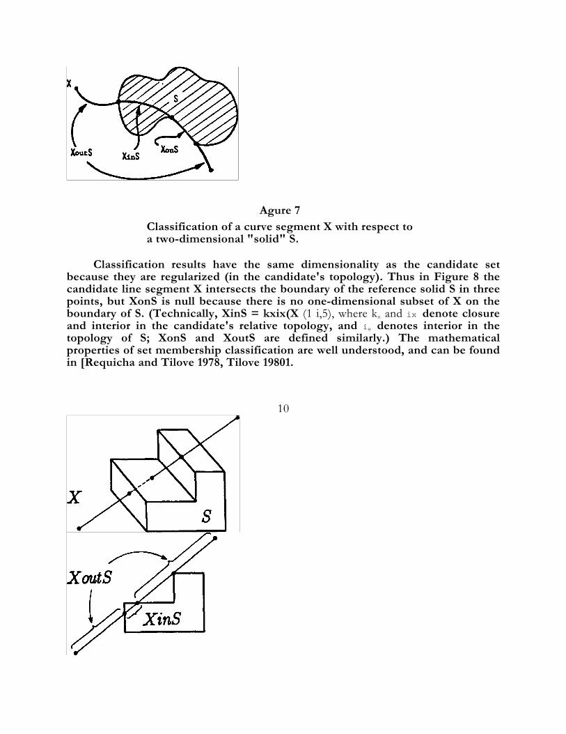
On/on ambiguities can be resolved by adding neighborhood information to the classifications. The neighborhood with radius R of a point p with respect to a solid S, denoted N(p, S; R), is the (regularized) intersection of a ball with radius R, centered at p, with the solid - see Figure 11. Applying regularized intersection with a ball B(p; R) to both sides of the expression S = A® B yields N(p, S; R) = N(p, A; R) ®N(p, B; R). Therefore the neighborhoods with respect to A and B can be combined to produce the neighborhood with respect to S. On/on ambiguities can be resolved by inspection of N(p, S; R), as shown in Figure 12. (It is shown in [Requicha and Tilove 1578] that to combine classifications it suffices to know the neighborhoods for almost all points of X - for example, the neighborhoods for all

but the endpoints of the segments in the examples above - and for small R; in the sequel we shall assume that R is sufficiently small and ignore it.)

13

N(p,s;R) = B(p;R) rrs

Agure 11 Neighborhood with radius R of point p with respect to solid S.

14

8 P N(RA) U

N(p,B) N(p,S)

N(p,A) N(p, S) U

N(pqB)

Figure 12 on Resolving on/on ambiguities by using neighborhood information.

The foregoing discussion shows that classifications cannot be combined because of on/on ambiguities, but that if one defines augmented classifications per XwrtS = (XinS, (XonS, N(XonS, S)),XoutS) by including neighborhood information for the boundary segments, these can be combined. (Henceforth we consider only augmented classifications, and drop the qualifier "augmented" for simplicity of language.)

The main computational requirements for combining classifications are the following. Representations for subsets of X, and for neighborhoods of points of X with respect to S. Algorithms for Boolean operations on subsets of X, and for Boolean 15

operations on neighborhoods. Representations and algorithms for subsets of X depend strongly on the

dimensionality of X. If X is a line or curve segment defined by a parametric equation p = p(t), it is convenient to represent subsets of X by sorted lists of parametric intervals (to, tl), (t2, t3), ... Boolean operations on lists of parametric intervals are easy to perform by using algorithms similar to the "merge" portion of the well-known "merge-sort" algorithm [Aho, Hopcroft and Ullman 1974]. For higher-dimensional candidates the situation is much more complicated. For example, if X is two-dimensional (a bounded subset of a surface) it can be represented by its bounding edges, but Boolean operations require two-dimensional versions of the boundary merging algorithms to be discussed in Section 3.

Neighborhood representations and algorithms are discussed in the following subsection.

2.3 Representing and Combining Neighborhoods

Two primary methods are known for representing neighborhoods: -

implicitly, through incidence and adjacency data in BReps, and -

explicitly, as explained below. In this paper we focus on explicit representations, which are used in the PADL-1, PADL-2 and GMSolid [Boyse and Gilchrist 1982] modellers but have not been discussed previously in the literature.

Neighborhoods for points that are in the interior or in the complement of a solid are "full" (a whole ball) or empty, and therefore can be represented easily. For points on the boundaries of solids it is useful to distinguish the following three cases. (Case designations are Rochester jargon.)

S -D Face ne i ghborhoods ( i . e . , neighborhoods for points in the interior of a solid's faces with respect to the 3-D solid). Observe in Figure 13 that the neighborhoods are specified completely by an answer to the question: On what side of the face is the solid's "material"? A simple representation can be constructed as follows. Associate with each surface (plane, cylinder, etc.), by convention a positive side; for example, convention that the "inside" of an unbounded cylindrical surface is its positive side. Then

16

represent the neighborhood of a face by a bit (or sign) that indicates whether the material is or is not in the positive side of the surface in which the face lies. an the jargon such a representation is sometimes called a "normal sign" or a "side bit".)

S -D Edge neighborhoods (i.e., neighborhoods for points in the interior of a solid's edges with respect to the 3-D solid). Figure 14 shows that neighborhoods can be represented by the "sectors" that contain material around the edge. Each sector can be represented in terms of the surfaces that bound it, plus normal and tangent signs. A surface separates 3space into two half-spaces, and a curve separates a surface into two halfsurfaces; the normal and tangent signs serve to distinguish between these half-spaces or half-surfaces. Note that edges shared by more than two faces (when a solid's boundary is not a 2-manifold [Requicha 1977]) can be accommodated by using lists of sectors rather than single sectors: (The representations just described are very similar to those used in GMSolid; PADL-2 uses slightly different representations, and PADL-1 uses another scheme that caters only to manifolds.)

S-.D Vertex neighborhoods (i.e., neighborhoods of vertices of a solid with respect to the 3-D solid). These can be represented by "generalized sectors", each usually bounded by at least three surfaces. Vertex representations are complex, difficult to manipulate, and not needed in most of the algorithms to be discussed later. < >

<2> For the representations just discussed to be useful, a solid's boundary must be segmented into faces and edges such that all interior points of a single face have the same neighborhood representation, and similarly for edges. This "constant neighborhood" condition is a subtlety that is satisfied in all BReps known to us, but potentially can cause problems for complicated, "sculptured" objects.

17 Neighborhoods with respect to faces, rather than solids, sometimes are

useful. The following two cases can be distinguished. • 8-D Edge neighborhoods (i.e., neighborhoods for points in the interior of edges

of a solid's face with respect to the face). These are the 2-D analogs of 3-D face neighborhoods, and can be represented by normal signs or side bits that indicate on which side of the edge is the face (Figure 15). Often this information is encoded by assigning an orientation to the edges.

• 2-D Vertez neighborhoods (i.e., neighborhoods of vertices of a face with respect to the face). These are the 2-D analogs of 3-D edge neighborhoods and can be represented by sectors, bounded by curves (Figure 16).

Agure 18

3-D Face neighborhoods.

~, - -Su rf (Fl )

P

-r - nl Surf ( F 2 )

t 2

< Surf (Fl)v ti 9 nl > , < Surf ( F ' 2 )q t 2 , n 2 > Moure 24 3-D Edge neighborhoods.

P

Figure 25 2-D Edge neighborhoods.

19

Agure 16

2-D Vertex neighborhoods.

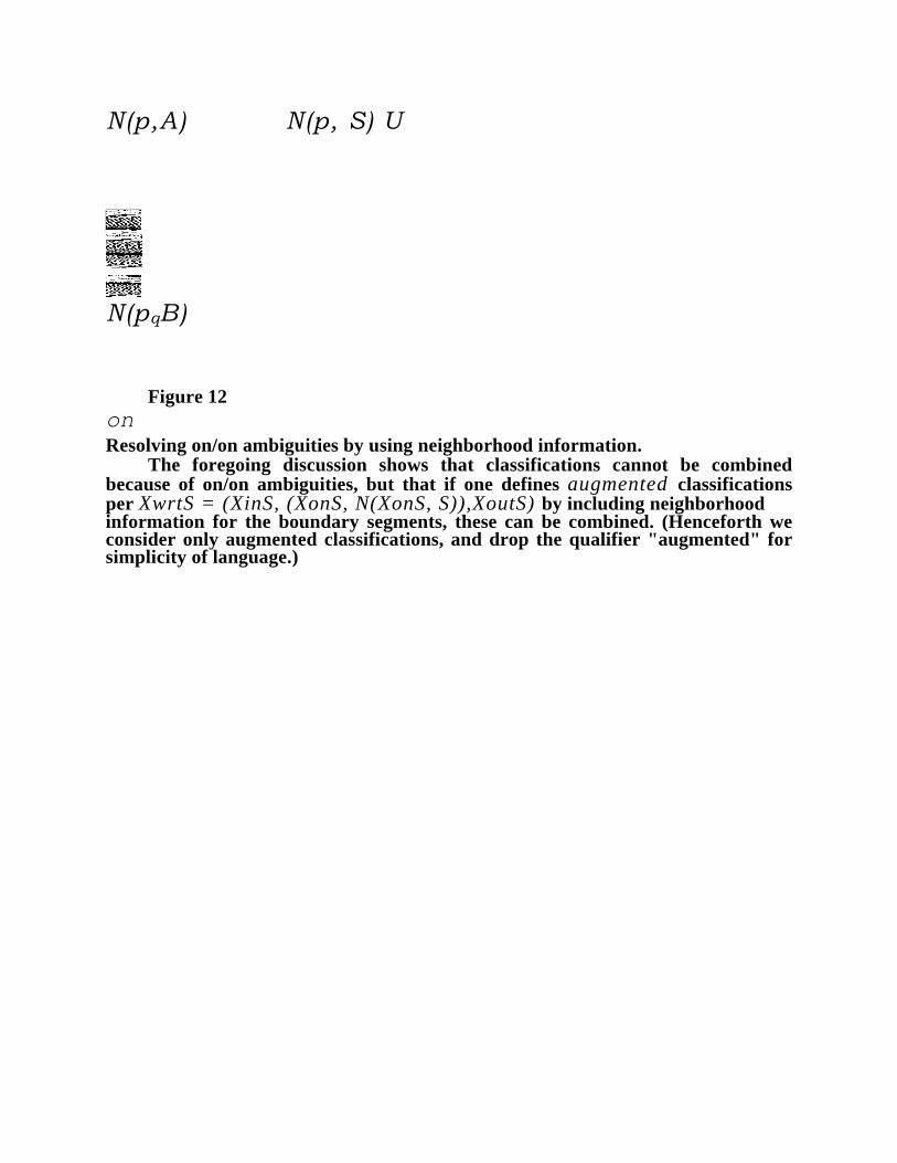
In the remainder of this paper it is assumed that BReps contain the explicit neighborhood representations required by the algorithms under discussion. It is worth noting that 2-D edge neighborhoods can be inferred from their 3D counterparts, as suggested in Figure 17, and that explicit neighborhood representations are computable from the incidence and adjacency information contained in "data-rich" BReps such as the winged-edge representations (Baumgart 1974).

20

3-D

Figure 27 Inferring 2-D neighborhoods from 3-D neighborhoods.

Combining 3-D face neighborhoods is straightforward. It amounts to performing logical operations (and, or, not and) on side bit representations, as shown in Figure 18. (Recall that two face neighborhoods only have to be combined when the faces overlap, and therefore there are only two possible cases, which are those shown in the figure.)

21

A l 1 ' ` B A f l ' ` B A - * B t p

o r and not and

Pygure 18 Combining 3-D face neighborhoods.

Combining edge neighborhoods is a relatively complex operation. Figure 19 shows a planar cross-section of the neighborhoods of an edge with respect to two solids A and B. The plane is normal to the edge, which is the intersection of four distinct surfaces and is normal to the paper. It should be clear from the figure that neighborhood combination amounts essentially to sorting (ordering) surfaces around the edge and selecting the appropriate sectors, according to the Boolean operation being performed. In PADL-2 the procedures for combining edge neighborhoods compute the curves of intersection of the relevant surfaces with a plane normal to the edge, and attempt to sort these curves by angle about the edge, by using straight-line (tangent) approximations; if this approach fails because several curves have the same tangent, higher-order information (curvature, etc.) is used for the sort. 22

Agure 19 Combining 3-D edge neighborhoods. 2.4 The Divide-and-Conquer Paradigm for Classification on CSG

Consider first the specific problem of classifying a line segment with respect to a solid represented by CSG, and assume that line segments are represented by parametric intervals and neighborhoods are represented explicitly, as described above. The divide-and-conquer paradigm, which has been found useful for many CSG-based algorithms, leads to the recursive classification procedure shown in Figure 20. (Algorithms in this paper are written in a dialect of pidgin Pascal;

23 procedures are assumed to return values.)

Le&S RighLS

procedure ClassLine3D(L,S) ff S is a primitive

then ClassLine3DwrtPrim (L,S)

she CombLine3D (C1assLine3D (L,Left.5), ClassLine3D (L,Right.S), OP.S)

Figure 20 Procedure for classifying a line with respect to a solid represented by CSG.

The procedure ClassLine3D of Figure 20 assumes that there are procedures for classifying lines with respective to primitives, and procedures for combining classifications. Primitive classifiers are easy to write when primitives are cuboids, cylinders and the like. More complex primitives require procedures for finding the common roots of the equations that define the line and the primitive's surfaces. CombLine3D is the procedure for combining classifications (and neighborhoods) discussed in Sections 2.2 and 2.3.

Observe that ClassLine3D will also classify curves with respect to solids, provided that the appropriate primitive classifiers and neighborhood combiners are available; the bulk of the CombLine3D procedure need not be changed if curve segments are represented by parametric intervals.

The divide-and-conquer paradigm can also be applied to face/solid 24

classification, and leads to a high-level algorithm very similar to that of Figure 20. However, the required CombFace3D procedure is complex because it must perform Boolean operations on face subsets, as noted earlier. This makes the approach less atractive than edge-based face classification, to be discussed in Section 3 in the context of boundary evaluation and merging.

2.5 Classification Algorithms for BReps Consider again line/solid classification, but assume now that the solid is

represented by its boundary. The basic algorithm intersects the line with the faces of the solid and determines the type of transition at each intersection point (e.g., out -i in, at point P3 of Figure 21) by examining the point's neighborhood. Classification status can change only at such intersection points, but need not change at all of them; for example, there is no change at point P5 in the figure (out -i out).

Intersections points are computed by a three-step procedure. First, intersect the unbounded line in which the segment L lies with the surface in which a face of S lies. This can be done by a numerical procedure, typically by substituting the parametric equation of the line in the implicit equation of the surface and solving for the parameter value t of the point(s) of intersection. The second step is point/segment classification to determine if an intersection point is within the line segment. The third step is point/face classification to determine if a point of intersection is within the face. (Note that faces can be very complex, e.g., polygons with many edges, concavities and holes.) PZ and Ps in Figure 21 are not points of intersection of the line segment L with the faces of S and therefore must be discarded, although they are the intersections of L with the surfaces in which the faces lie.

Figure 22 Classification of a line segment L with respect to a solid S represented by a BRep.

Transitions at intersection points are easy to determine for points in the interior of faces. For polyhedral solids it suffices to compare the direction of the line with the direction of the inward pointing normal at the intersection point, as shown in Figure 22. The inward normal is easy to obtain from the equation of the face's surface and the 3-D face neighborhood representation (normal sign).

26

o u t - + i n

Agure 22 Determining the type of transition at an intersection point in the interior of a face.

Intersection points, however, may lie within edges or be vertices of the solid. We refer to these cases as singularities, and to the operation of determining transition types by examining the points' neighborhoods as resolution o f singularities. (This terminology is borrowed from [Kalay 1982], which contains an extensive discussion of singularity resolution for polyhedra.) Edge singularities can be resolved by comparing the direction of the line with the 3-D edge neighborhood representation, as suggested in Figure 23.

27

out -+ out out -+ in

Resolving singularities for intersection points in the interior of edges. Vertex singularities are harder to resolve, but can be avoided, as shown in

Figure 24. To determine the type of transition at a vertex singularity simply classify the midpoints of the two line segments immediately adjacent to the vertex (or two other convenient points in the segments). The transition can be inferred trivially from these classifications. Observe that the midpoints cannot be vertices, although they may lie within edges. Classification of a point P with respect to a solid S represented by its boundary is illustrated in Figures 25 and 28. The algorithm is a simplified version of line/solid classification for a semi-infinite ray emanating from the point P. Intersections between the ray and the solid are computed through ray/face comparisons, as explained above. Because any ray through P will do, in the unlikely event that the closest intersection point Pe is a singularity (and is dintinct from P), simply select randomly another ray and try again. (We believe that the algorithm just described is numerically more robust than the better-known method, which consists of counting the number of intersections between a ray through P and the solid; other point/solid classification algorithms are described in (Kalay 1982].)

28

Classif)r midpoints

Agure 2 Avoiding vertex singularities by classifying segments' midpoints.

Agure 25

Point/solid classification by ray casting.

29 procedure ClassPoint3D(P,S)

R •- Ray through P

i f R n S = 0 then P is 'out'

she Pe • - Intersection R n S closest to P 1f P = P then P is 'on' e

doe i f P , is a singularity then select another ray fit re-start

she Examine Nbhd3D(P,, S) to determine transition type 8a infer classification for P.

Agure t6 An algorithm for classifying a point with respect to a solid represented by a BRep.

A complete algorithm for line/BRep classification is shown in Figure 27, For simplicity, it is assumed that the initial point of the line segment is out of $. (If this is not the case, extend the segment as needed, classify the extended segment, and infer the classification of the shorter, initial line segment.) The maim components of the procedure were described previously, and a few additional details are given here.

30 precedwe ClassL3ne3D(L,S)

fb ce F of S do (face loop) r ea& fait L 0 Surf(F) then P •- L

f1 Surf(F) MI •- ClassPoint2D (P,F)

if CVaj Z= 'outF' then Discard (P) she AddTolntList (P,Nbhd3D(P,S)) end (case)

the Do nothing end (face loop)

Sort IntList by t-value 8a merge coincident P's fbr each P{ do

Examine Nbhd3D(Pi, S) to determine transition type {Insert code to avoid vertex singularities} Wer classification for (P;, Pi+l) and (for)

Figure 27 Algorithm for classifying a line segment with respect to a solid represented by a BRep.

1) When L lies in the surface of some face F of the solid, the face is ignored in the face loop of Figure 27, because the required intersection points are obtained from intersections of L with other faces, as shown in Figure 28.

2) Point classification with respect to a face F is a 2-D analog of the ClassPoint3D procedure of Figure 26; briefly, cast through P a ray lying in the surface o f F, determine its intersection with the edges of F, and examine the 2-D neighborhood of the closest intersection.

3) Points of intersection of the line with the faces are added to an IntList 31

together with their neighborhoods with respect to S; these neighborhoods can simply be copied from the BRep of S.

P1 and P2 computed when L is tested against the hatched faces

Agure 88

Line lying in a face of S.

The main computational requirements for classification of line segments with respect to solids represented by BReps can be summarized as follows. Procedures to intersect the line with the surfaces of the solid. (These are equation solvers, which may exploit closed-form solutions or use iterative numerical methods.)

Procedures to intersect lines lying in the solid's surfaces with lines in which the edges lie, to classify the resulting intersection points with respect to the edges, and to examine 2-D neighborhoods. (All of these are needed to support point/face classification.) Procedures to examine 3-D neighborhoods and determine transition types.

32 The basic algorithm described in this section can also be used to classify

curves with respect to curved solids, but the required procedures analogous to those just listed are much more complex for curved entities than for lines and polyhedra.

It is easy to design by analogy with ClassLine3D a procedure ClassLine2D for classifying lines with respect to "faces" (i.e., bounded subsets of surfaces). Indeed, a simplified form of ClassLine2D was used above for point/face classification by ray casting.

C1assLine3D also generalizes to face/solid classification, at the expense of some added complexity. Recall that ClassLine3D operates by generating the intersection points of the candidate with the solid's faces, sorting these to produce subsets (segments) of the candidate that are guaranteed to have constant classification (e.g., to be wholly in), and inferring classifications for each subset by examining neighborhoods or by classifying a point within each segment (thereby avoiding singularities). The 3-D analog generates the line segments of intersection of the candidate with the solid's faces, organizes these segments so as to bound subsets ("regions") of the candidate, and infers classifications for the regions through neighborhood analysis or point classification. s. Boundary Evaluation and Merging

3.1 The Generate-and-Test Paradigm for Faces A boundary representation for a solid S can be computed by the algorithm

shown in Figure 29, which is an instance of the familiar generate-and-test paradigm of Computer Science.

Generate a sufficient set of tentative faces F

for each F do FwrtS f- ClassFace3D (F,S) AddToBRep (FonS) end {do}

Figure 29

Generate and classify tentative faces.

A set Fj of tentative f ace8 is 8u f f icient if U; Fi D 8S, Where 8S denotes the boundary of the solid S. The algorithm of Figure 29 starts with a set of faces that are guaranteed to include the solid's boundary, and discards those portions that are not on the solid.

Sufficient sets of tentative faces can be generated by using (recursively) the basic fact 8(A ® B) C (8A U 8B), which is intuitively plausible and easy to prove mathematically [Requicha and Tilove 1978]. The following are examples of sufficient sets.

1) The faces of A and the faces of B.

2) The surfaces in which the faces of A and B lie (or some convenient subsets

34 of such surfaces that include the faces of A and B).

3) The faces of all the primitives in a CSG representation of S.

4) The surfaces in which the faces of all the primitives of S lie. The first two of these sets lead to incremental algorithms, while the last two

lead to non-incremental algorithms. Tentative face generation, therefore, is straightforward. The main problem is to classify tentative faces with respect to S = A (& B. Several approaches can be used:

Classify faces with respect to S by divide and conquer on CSG. This involves face/solid classification on CSG, which is not very attractive as we saw in Section 2.4.

Classify faces with respect to A and B by algorithms that operate on BReps, and then combine the classifications. (This approach is very similar to the next one.)

Seek directly the bounding edges of FonS by using a generate-and-classify paradigm for edges.

The remainder of Section 3 focuses on the third of these approaches, which is the most common. Until now we have relied on intuition, and have not defined precisely what is meant by faces, edges and vertices. Before embarking on a discussion of edge-based algorithms, we must be more careful. The edges we seek must bound faces, and therefore depend on the definition of "face". Many definitions are possible [Silva 1981], but only so-called maximal faces are considered in this paper, because they are practically useful (essentially the faces of GMSolid and PADL-2 are maximal), and they simplify the discussion of boundary evaluation algorithms. They are defined informally as follows.

A maximal face is the largest 2-D subset of the boundary of a solid that lies in a single surface (plane, cylinder, etc.) and whose interior points have "constant

neighborhood". The constant neighborhood condition stipulates that the solid must be only on one side of the face's surface in the immediate vicinity of the face. For example, the hatched regions in Figure 30 correspond to two faces because the normal signs are not the same for the two regions. (Maximal faces need not be connected, and therefore the regions in the figure would constitute a single maximal face if they had constant neighborhood.)

35

Agure 90 Two subsets of a single surface that are not a

maximal face because their neighborhoods are not ' constant.

3.2 The Generate-and-Teat Paradigm, for Edges The basic algorithm is shown in Figure 31. In essence, it classifies the

tentative edges in a sufficient set and discards edge segments that are not on the solid's boundary. It also discards, through a "2-D test" (the SiugleSurf procedure), tentative edge subsets that are on 83 but are not boundaries of maximal faces. Figure 32 illustrates the 2-D test, and shows that edge segments to be discarded are characterized by neighborhoods containing a single surface.

36 Generate a sufficient set of tentative edges

for each tentative edge R do EwrtS •- ClassEdge3D (E, S) N SingleSnrf(Nbhd3D(RonS, S)) then Discard (E) she AddTbBRep(EonS) and (for)

Figure 92 Generate and classify tentative edges.

E = E on S, but not an edge o f A -*B Nbhd3D(E, S ) F

Agure 92 Tentative edge E is on 8S, where S = A *B, but does not bound a maximal face of S and is discarded by the 2-D test.

Two main problems remain: how to generate tentative edges, and how to classify them. The edges of a solid S = A ® B are subsets of edges of A and B - called self edges in Rochester jargon -- and of cross edges, i.e., intersections between faces of A and faces of B - see Figure 33.

38 face F

Solid A

Solid B face G

Agure 93

Self edges and cross edges are a sufficient set. Self edges are available in the BReps for A and B, and therefore self edge

generation is trivial. The classifications (including neighborhoods) of the self edges of a face F of solid A with respect to A are known. Therefore the edges of F can be classified with respect to S by classifying with respect to B, using either CSG or BRep algorithms, and combining with the known classifications with respect to A, as explained in Section 2. Similar remarks apply to the self edges of B.

Consider a face F of A and a face G of B, and assume that they do not overlap over a 2-D region. It is easy to see that (the closure of) the intersection of the (2-D) interior of F with the interior of G is either empty or it is an edge of S. Therefore cross edge classification is trivial if "minimal" cross edges are generated by intersecting the interiors of non-overlapping faces of A and B. Unfortunately, generation of minimal cross edges is difficult because the faces of A and B can be arbitrarily complex. The two common approaches to cross edge generation and classification both begin with "oversized" cross edges, generated by intersecting either the surfaces in which the faces lie or some convenient subsets of these surfaces that are guaranteed to enclose the faces.

The first approach consists simply of generating oversized cross edges and classifying them with respect to S either by divide-and-conquer on CSG or by using BRep algorithms, as explained in Section 2.

39 The second approach also generates oversized cross edges but "trims" them

through edge/face operations, as shown in Figures 34 and 35. Observe in Figure 35 that the segment EonS can be discarded because it is a self edge, and therefore will be processed in the self edge loops of the algorithm.

E •- F' n d (F, :> F, G' =) G} {Oversized cross edge}

E'wrtF ~- ClassEdge2D (E, F)

SwrtG ~- ClassEdge2D (Z, G) M-+-RimPrf jBinG (Minimal cross edge) Eons *-- M

{f?i : regularized intersection in 1-D}

Rgure 84 Algorithm for generating and classifying a cross edge through edge/face operations.

40

Agure 85 Edge/face operations.

Two complete algorithms are shown in Figures 36 and 37. The algorithm of Figure 36 is a simplified version of the incremental boundary evaluator of early versions of PADL-2. (Newer versions use algorithms that exploit spatial locality [Tilove et al. 1984].) It classifies all the tentative edges by divide and conquer on CSG (Section 2.4) and combines classifications by the CombEdge3D procedure of Section 2.3. (In PADL-2 the oversized cross edges are generated from faces of primitives, which are easy to intersect.) 41

for each face F of A do

fbr each self edge E of F do EwrtA •- E, Nbhd3D(E, A) EwrtB ~- CIsssEdge3D(E, B) EwrtS ~- CombEdge3D (EwrtA,EwrtB, Op.S)

V not SingleSnrf(Nbhd3D(EonS, S)) then AddToBRep(EonS) end (self-edges of A loop)

fbr each face G of B do (cross edges)

if Surf(G) 0 Surf (F) then

E +- F n G {F' D F, G' D G) SwrtS •- CLssEdge3D(E, S) if not SingleSurf (Nbhd3D(EonS, S)) then AddToBRep(EonS) end {first if}

end (cross edges loop) end (faces of A loop)

for each face G of B do . . . self edges

Agure 96

A simple PADIrstyle algorithm.

The algorithm of Figure 37 is a simple boundary merger, using edge/face operations. It classifies self edges by using the ClassEdge3D procedure for BReps discussed in Section 2.5, and processes cross edges through edge/face classification. ClassEdge2D is a 2-D analog of the 3-D procedure for BReps discussed in Section 2.5. It avoids vertex singularities and therefore does not require 2-D vertex neighborhoods, but requires 2-D edge neighborhoods. We assume that these exist in the BReps for A and B; the algorithm produces 2-D neighborhoods for the BRep of S by inferring them from their 3-D counterparts (see Section 2.3, especially Figure 17).

42

for each face F of A do

hr each self edge E of F do EwrtA ~- E, Nbhd3D(E, A) EwrtB ~- C1assEdge3D(E, B) EwrtS ~- CombEdge3D(EwrM, EwrtB,Op.S) V not SingleSurf(Nbhd3D(EonS, S)) then Infer Nbhd2D(EonS, NewF) AddTbBRep(EonS)

end (then)

and (self edges of A loop) fbr each face G of B do (cross edges)

if Surf(G) 0 Surf (F) then C *-- Surf(F) n Surf(G) CwrtF ~- ClassEdge2D(C, F) CwrtG C1assEdge2D(C, G) E +-- CsnF n* CinG Nbhd3D(E,Al ~- Copy from BRep(A) NbhdaD(E, B) •-- Copy form BRep(B) Nbhd3D(E, S) •- CombNbhd3D(Nbhd3D E,A), Nbhd3D(E, B),Op.S) EwrtS •- E, Nbhd3D(E, S) {E = EonS7 if not SingleSurf(Nbhd3D(E, S)) then

Induce Nbhd2D(E, NewF) AddToBRep(E) and (then)

end (top if) and (cross edges loop)

and (faces of A loop) for each face G of B do 0.. w1t edges

Agure 37 A simple algorithm using edge/face classification.

43 3.3 Efficiency Improvements

The simple algorithms of Figures 36 and 37 are slow. Their efficiency can be improved by several short cuts, which avoid unnecessary calculations, and by general performance enhancement techniques that exploit spatial locality in geometric computations.

A first short cut is fairy obvious. The face loops in the algorithms of Figures 36 and 37 traverse each self edge at least twice. This can be avoided by marking edges or by a similar "book keeping" technique.

A second short cut is more subtle. New vertices may be computed several times, as suggested in Figure 38, and these computations are expensive, especially for modellers that support objects with curved surfaces. Re-computation can be avoided simply by "remembering" that vertices have already been found, but vertex information can also be used to infer self edge classifications from cross edge classifications or vice-versa, as explained below.

V = (self edge El of F l) n G

V = (Cross edge E2 = Fl n G) n F2

V = (self edge El) n (cross edge E2)

V = SUFI) n SurqF2) n Surf(G)

Figure 88

The new vertex V may be computed several times.

Algorithms that classify cross edges by edge/face operations intersect each oversized cross edge C with all the edges of each face - see Figure 39. When a vertex V is found by intersecting the cross edge C with the self edge E, V can be added to the intersection lists (see Section 2.5) of C and also of E. After all cross edges have been classified, the intersection lists for all self edges are available, and

the classification of the self-edges can be inferred by sorting the intersection lists and examining neighborhoods as explained in Section 2.5. This short cut complicates the code considerably and has its subtleties. For example, generating cross edges by intersecting the interiors of faces is no longer sufficient, because there is no separate self edge loop to take into account faces that meet at a common edge and other similar situations.

45

Agure 88

Using cross edges to infer self edge classifications.

Conversely, classifications for cross edges can be inferred from self edge classifications because all vertices of a polyhedral S must lie in self edges of A or B. In fact, a vertex of S must lie in at least three faces of S, and these are subsets of either the faces of A or B; it follows that at least two of the faces must belong to one of the solids A or B and therefore V lies in the self edge defined by those two faces (see Figure 40). Observe that this argument is correct for polyhedral solids but may fail for curved objects; indeed, cross edge classifications may not be inferable from self edges for curved solid domains (think of spheres, for example).

46

Figure 40

Vertices of S must lie in self edges of either A or B.

The two short cuts just discussed cannot be expected to decrease running time by more than a factor of three or four. Order of magnitude improvements in the average performance of the algorithms are achievable through techniques that exploit the spatial locality inherent in most of the geometric computations required for boundary evaluation and merging [Tilove 1981b]. These techniques are based on the following simple observation. Boundary evaluation and merging algorithms must intersect many geometric entities; for example, all faces of A are compared with all faces of B in the algorithms of Figures 36 and 37 to generate tentative edges. But typically each face only has non-empty intersections with a few other faces that occupy a nearby region of space. Therefore most of the comparisons can be avoided by using disjointness information to cull faces that cannot possibly intersect. Disjointness information can be acquired by using spatial grids, hierarchical decompositions of space, scanning algorithms, and so forth. Discussion of these techniques is worth a separate paper. Here we simply want to emphasize their importance, because they are essential for achieving reasonable performance in current-technology solid modellers.

47 3.4 A Brief Survey of Known Approaches

The various approaches to boundary evaluation and merging that have appeared in the literature or are otherwise known to us can be characterized as follows, by using the concepts discussed earlier in this paper. < 8

1) Classify self and cross edges by divide and conquer on CSG - GMSolid [Boyse 1978], which avoids recomputing vertices, and early versions of PADL-2. (A non-incremental version of this algorithm is used by PADL1, and recent releases of PADL-2 use algorithms that combine non-incremental and "boundary editing" techniques [Tilove et at. 1984].) An interesting feature of the approach is that it relies only on two geometric

utilities: surface/surface intersection to generate tentative edges, and edge/solid classification on CSG.

2) Classify self edges via BRep algorithms, and cross edges by edge/face operations - GMSolid.

3) Classify faces by using surface/solid classification for BReps - [Putnam and Subrahmanyam 19821.

4) Classify faces by using BRep algorithms; specifically, generate cross edges, classify them with respect to faces, decompose faces into subsets, and infer classifications for the subsets avoiding singularities - [Franklin 1982, Turner 1978].

5) Classify cross edges and infer self edge classifications by BRep algorithms; resolve singularities and maintain BRep connectivity information - BUILD [Braid 1979] and GLIDE [Kalay and Eastman 1980].

fi) Classify self edges and infer cross edge classification by BRep algorithms - GWB [Mantyla 1982], Synthavision [Steinberg 1982].

<3> We apologize to authors for possible misinterpretations of their work.

48 Readers are referred to the original reports and articles for more details on the

approaches above. The literature tends to address algorithmic description at a lower level than in this paper, and to intersperse short cuts, efficiency "tricks", and implementational details through the basic algorithm description; some of the original articles gloss over important characteristics of the algorithms (e.g., whether they operate correctly on solids with overlapping boundaries).

3.5 Topics Not Addressed in this Paper For reasons of simplicity and space, several important topics were ignored in the foregoing exposition.

BRep structure. The algorithms described earlier produce BReps that may be "dirty" with repeated or overlapping edges, and that have no explicit connectivity information. BRep "cleaning" is easy to accomplish in a second stage, and connectivity links also can be computed after the boundary is evaluated. Maintaining connectivity during boundary evaluation or merging can also be done but seems to complicate the logic substantially.

Non-maximal faces. Non-maximal faces are preferred by many designers of BReps. The algorithms presented can be modified, primarily by using more elaborate 2-D tests, to produce non-maximal faces.

Computational complexity. The worst case complexity of the algorithms can be analyzed by techniques similar to those in [Tilove 1981a]. The algorithms run in polynomial time, of course, but the exponents are relatively high. Experimental data show that the worst case bounds are essentially worthless because they are very pessimistic. Unfortunately, the average complexities of the algorithms are unknown.

Implementation sand system integration. Successful implementation of the algorithms in a modelling system requires careful design. Two examples of issues that must be addressed are: (1) data sharing amongst BReps for subtree objects in dual CSG/BRep modellers, and (2) behavior of BReps when objects are edited. Related algorithms. Similar algorithms can be used to produce wireframes for display, to detect null objects - an important geometric utility for studying collisions and detecting object equality [Tilove 1981b, 1984] -and to update BReps or wireframes when CSG representations are edited [Tilove 1981b, Tilove et al. 10841.

49 4. Smeary and Concluding Remarks

This paper discusses algorithms for converting CSG representations into BReps, and for merging BReps of solids that are combined by Boolean operations (i.e., regularized set operations). These algorithms are amongst the most fundamental and delicate software components of state-of-the-art solid modellers.

Set membership classification and neighborhood manipulation are key unifying notions, which serve to explain the high level structure of known algorithms. Boundary evaluation and merging algorithms operate by classifying faces and edges with respect to solids, and by combining classification results. Because combining classifications involves Boolean operations, the algorithms essentially "recurse in dimension", i.e., compute Boolean operations on higher dimensional entities (solids) through Boolean operations on lower dimensional entities (faces, and especially edges because one-dimensional Boolean operations are computationally straightforward).

Several approaches are known, and undoubtedly others are possible. Unfortunately, data or theoretical analyses for assessing the relative merits of the different approaches do not exist, as far as we know. The following are some of the important but unresolved issues. Is classification on CSG simpler and numerically more robust' than on BReps? Is it less efficient? Is avoiding singularities simpler and more robust than resolving singularities? Is it less efficient? Do short cuts inherently complicate the logic of the algorithms? Are they worth implementing?

Are explicit neighborhood representations simpler to maintain and more amenable to parallel algorithms than implicit representations imbedded in BRep connectivity information? Which approach is more robust and efficient?

Our opinions (biases?) on these topics can be inferred from the design of the PADL-2 boundary evaluators, but they should be viewed as personal opinions based on insufficient data, and no more than that. Most of the issues listed above are concerned with efficiency and numerical stability. We suggest that boundary evaluation and merging algorithms would profit significantly from the attention of theoretical computational geometers and numerical analysts, who might find ways

50 to analyze current algorithms and design better ones.

5. Aclmowledgements and Historical Notes Additions and subtractions of "shapes" have long been recognized as

important for defining solid objects. Even traditional drafting texts (see e.g. [Schneerer, p. 761) state that mechanical parts are conceptually built by combining simple shapes such as blocks, cylinders, cones and spheres. Boolean operations on solids can be traced to the computing literature of the 1960's (e.g., [Roberts 1963, Gutterman 1964]). CSG representations were used in the early versions of Synthavision [Goldstein 1971] and TIPS [Okino, Kakazu and Kubo 19731, but these systems operated directly from CSG, without computing boundaries. The first boundary merging algorithms appear to be those of BUILD-1, a system designed and implemented by Ian Braid in a Cambridge Ph.D. thesis in the early 1970's [Braid 1973]. Braid's algorithms did not support Boolean operations in their full generality; they required that objects to be combined share faces in specific ways, and so forth. The first fully general boundary evaluation algorithms appear to be those in the version of PADL-1 demonstrated publicly in 1976. Since then many other such algorithms have been implemented, although the generality and correctness of some of them are unclear.

The view presented in this paper evolved over the past decade at the Production Automation Project of the University of Rochester. Point membership classification was introduced by Requicha in early 1975 as a didactic device to explain the then-mysterious notion of representation completeness (or unambiguity). Voelcker and Requicha posed the problem of classifying points with respect to CSG solids by divide and conquer to engineering students enrolled in the 1975 version of EE458 "Geometric modelling and engineering graphics". It was soon discovered that classifications could not be combined, and the problem was resolved by Requicha through the introduction of neighborhoods. Voelcker generalized the notion of classification and made the crucial observation that boundaries could be computed by tentative edge classification. The first boundary evaluator based on these notions was designed and implemented by Voelcker in the Summer of 1975, and was extended to curved objects (cylinders) by Tilove also in 1975. (Two earlier approaches to boundary evaluation had been attempted at

Rochester with limited success; one operated by symbolically expanding strings corresponding to the formulae for combining solid boundaries [Requicha and Tilove 1978], and the other used an algorithm related to what we now call face classification by divide and conquer.) The mathematics of set membership classification was worked out by Requicha and Tilove in 1975-1976. PADL-1's

51 boundary evaluator was (and is) non-incremental. An incremental algorithm was designed in 1976 by Voelcker, and a version of it was implemented in an early version of PADL-2 in the late 1970's. Recent versions of PADL-2 use algorithms that combine the incremental and non-incremental approaches and exploit spatial locality [Tilove et al. 1984].

REFERENCES

[Aho, Hopcroft and Ullman 1974] A. V. Aho, J. E. Hopcroft, and J. D. Ullman, The Design and Analysis of Computer Algorithms. Reading, MA: Addison-Wesley, 1974. [Baumgart 1974] B. G. Baumgart, "Geometric modelling for computer vision", Report STAN-CS-74-463, Stanford Artificial Intelligence Lab., Stanford Univ., 1974. [Boyse 1978] J. W. Boyse, "Preliminary design for a geometric modeller", Report GMR-2768, Computer Science Dept., General Motors Research Labs., July 1978. [Boyse and Gilchrist 1982] J. W. Boyse and J. E. Gilchrist, "GMSolid: Interactive modeling for design and analysis of solids", IEEE Computer Graphics PY Applications, vol. 2, no. 2, pp. 27-40, March 1982. [Braid 1973] I. C. Braid, "Designing with volumes", Ph.D. Dissertation, University of Cambridge, U.K., 1973. [Braid 1979] I. C. Braid, "Notes on a geometric modeller", C.A.D. Group Doe. No. 101, Computer Laboratory, Univ. of Cambridge, U.K., June 1979.

[Brown 1982] C. B. Brown, "PADL-2: A technical summary", IEEE Computer Graphics &Applications, vol. 2, no. 2, pp. 69-84, March 1982. [Foley and van Dam 1982] J. D. Foley and A. van Dam, Fundamentals of Interactive Computer Graphics. Reading, MA: Addison-Wesley, 1982. [Franklin 1982] W. R. Franklin, 'Efficient polyhedron intersection and union", Floc. Graphics Interface '82, pp. 73-80, Toronto, Canada, May 17-21, 1982. [Goldstein 1971] R. A. Goldstein and R. Nagel, "3-D visual simulation", Simulation, vol. 16, no. 1, pp. 25-31, 1971. [Gutterman 1964] M. M. Gutterman, "APT numerical description study", Report No. 578-T45-10, I.I.T. Research Inst., Sandia Corp., 1964. [Kalay and Eastman 1980] Y. E. Kalay and C. M. Eastman, "Shape operations: An algorithm for spatial-set manipulations of solid objects", CAD - Graphics Lab., Carnegie-Mellon Univ., July 1980.

53

[Kalay 1982] Y. E. Kalay, "Determining the spatial containment of a point in general polyhedra", Computer Graphics & Image Processing, vol. 19, no. 4, pp. 303-334, August 1982. [Kedem and Ellis 1984] G. Kedem and J. H. Ellis, "Computer structures for doing curve-solid classification in geometric modeling", Computer Science Dept. and Production Automation Project, Univ. of Rochester, 1984. [Mantyla 1982] M. Mantyla, "Set operation algorithm of GWB", Report--HTKKTKO B48, Lab. of Information Processing, Helsinki Univ. of Technology, 1982. [Meagher 1982] D. Meagher, "Geometric modeling using octree encoding", Computer Graphics & Image I~ocessing, vol. 19, no. 2, pp. 129-147, June 1982. [Newman and Sproull 1979] W. M. Newman and R. F. Sproull, FKnciples of Interactive Computer Graphics. New York: McGraw-Hill, 2nd ed., 1979. [Okino, Kakazu and Kubo 1973] N. Okino, Y. Kakazu, and H. Kubo, "TIPS--1: Technical processing system for computer-aided design, drawing and manufacturing", in J. Hatvany, Ed., Computer Languages for Numerical Control. Amsterdam: North-Holland Pub. Co., 1973, pp. 141-150. [Putnam and Subrahmanyam 1982] L. K. Putnam and P. A. Subrahmanyam, "Computation of the union, intersection and difference of n-dimensional objects", Dept. of Computer Science, Univ. of Utah, 1982. [Requicha 1977] A. A. G. Requicha, "Mathematical models of rigid solid objects", Tech. Memo. No. 28, Production Automation Project, Univ. of Rochester, November 1977. [Requicha and Tilove 1978] A. A. G. Requicha and R. B. Tilove, `Mathematical foundations of constructive solid geometry: General topology of closed regular sets", Tech. Memo. No. 27a, Production Automation Project, Univ. of Rochester, June 1978. [Requicha 1980] A. A. G. Requicha, "Representations for rigid solids: Theory, methods, and systems", ACM Computing Surveys, vol. 12, no. 4, pp. 437-464, December 1980. [Requicha and Voelcker 1982] A. A. G. Requicha and H. B. Voelcker, "Solid modelling: A historical summary and contemporary assessment", IEEE Computer Graphics &Applications, vol. 2, no. 2, pp. 9-24, March 1982.

54 [Requicha and Voelcker 1983] A. A. G. Requicha and H. B. Voelcker, "Solid modelling: Current status and research directions", IEEE Computer Graphics 8 Applications, vol. 3, no. 7, pp. 25-37, October 1983. [Roberts 1963] L. G. Roberts, "Machine perception of three dimensional solids", Tech. Report 315, M.I.T. Lincoln Lab., Lexington, MA, 1963. [Schneerer 1967] W. F. Schneerer, Fl-ogrammed Graphics. New York: McGraw-Hill, 1967. [Silva 1981] C. E. Silva, "Alternative definitions of faces in boundary representations of solid objects", Tech. Memo. No. 36, Production Automation Project, Univ. of Rochester, November 1981.

[Steinberg 1982] H. A. Steinberg, "Overlap and separation calculations using the SynthaVision three dimensional solid modeling system", Proc. Conf. on CADICAM Technology in Mechanical Engineering, Cambridge, MA, pp. 13-19, March 24-26, 1982. [Tilove and Requicha 1980] R. B. Tilove and A. A. G. Requicha, "Closure of Boolean operations on geometric entities", Computer Aided Design, vol. 12, no. 5, pp. 219-220, September 1980. [Tilove 1980] R. B. Tilove, "Set membership classification: A unified approach to geometric intersection problems", IEEE ?bans. on Computers, vol. C-29, no. 10, pp. 874-883, October 1980. [Tilove 1981a] R. B. Tilove, "Line/polygon classification: A study of the complexity of geometric computation", IEEE Computer Graphics &Applications, vol. 1, no. 2, pp. 75-88, April 1981. [Tilove 1981b] R. B. Tilove, "Exploiting spatial and structural locality in geometric modelling", Tech. Memo. No. 38, Production Automation Project, Univ. of Rochester, October 1981. [Tilove 1984] R. B. Tilove, "A null object detection algorithm for constructive solid geometry", to appear in Comm. ACM. [Tilove et al. 1984] R. B. Tilove et al., "Efficient editing of solid models by exploiting structural and spatial locality", Tech. Memo. No. 46, Production Automation Project, Univ. of Rochester, 1984.

[Turner 1978] J. A. Turner, "An efficient algorithm for doing set-operations on 55 two- and three--dimensional spatial objects", Architectural Research Lab., Univ. of Michigan, 1978. [Voelcker et al. 19781 H. B. Voelcker et al., "The PADL-1.0 f 2 system for defining and displaying solid objects", ACM Computer Graphics, vol. 12, no. 3, pp. 257283, August 1978. (Proceedings Siggraph '78).