Technical Memo and Attachement A and B- SCA and … · Settlement ... • U.S. Army Corps of...
142
-
Upload
truongmien -
Category
Documents
-
view
216 -
download
0
Transcript of Technical Memo and Attachement A and B- SCA and … · Settlement ... • U.S. Army Corps of...


P:\Honeywell -SYR\444853 - Lake Detail Design\09 Reports\9.6 SCA IDS\App A - Tech Memo\Tech Memo.doc
M E M O R A N D U M August 11, 2009
To: Tim Larson, NYSDEC
From: Ed Glaza, Parsons
Subject: Sediment Consolidation Area (SCA) Civil and Geotechnical Technical Memorandum
This Sediment Consolidation Area (SCA) Civil and Geotechnical Technical Memorandum (Technical Memorandum) has been prepared on behalf of Honeywell International Inc. in accordance with the Remedial Design Work Plan (RDWP) for the Onondaga Lake Bottom Subsite (Parsons, 2009). The RDWP presents the activities necessary to complete design of the remedy selected in the Record of Decision issued by the New York State Department of Environmental Conservation (NYSDEC) and the United States Environmental Protection Agency Region 2 in 2005, and as set forth in the Consent Decree (United States District Court, Northern District of New York, 2007) (89-CV-815).
This Technical Memorandum is being submitted in advance of the SCA Civil and Geotechnical Initial Design Submittal (IDS) to facilitate NYSDEC’s review of the IDS and achievement of the overall project schedule. Preparation and submission of this Technical Memorandum allows NYSDEC the opportunity to review and provide comments on the following documents prior to their inclusion in the IDS:
• Attachment A – Basis of Design
• Attachment B – Subsurface Stratigraphy Model of Wastebed 13 for the Design of Sediment Consolidation Area (i.e., the Data Package).
To further facilitate NYSDEC’s IDS Review, the SCA Dewatering Evaluation Report will be submitted in advance of the IDS. The content and submittal schedule for the IDS will be in accordance with the RDWP.
REFERENCES
NYSDEC and USEPA. 2005. Record of Decision Onondaga Lake Bottom Subsite of the Onondaga Lake Superfund Site. Town of Geddes and Salina, Villages of Solvay and Liverpool, and City of Syracuse, Onondaga County, New York.
Parsons, 2009. Remedial Design Work Plan for the Onondaga Lake Bottom Subsite Prepared for Honeywell. March 2009.
United States District Court, Northern District of New York. 2006. State of New York and Denise M. Sheehan against Honeywell International, Inc. Consent Decree Between the State of New York and Honeywell International, Inc. Senior Judge Scullin. Dated October 11, 2006. Filed January 4, 2007. Order Number 89-CV-815. Syracuse, New York.

ONONDAGA LAKESEDIMENT CONSOLIDATION AREA
CIVIL AND GEOTECHNICALBASIS OF DESIGN
PARSONS
C:\SedimentConsolidationArea\Attach A - Basis of Design.doc December 4, 2009
ATTACHMENT A
CIVIL AND GEOTECHNICAL BASIS OF DESIGN

ONONDAGA LAKE
SEDIMENT CONSOLIDATION AREA
CIVIL AND GEOTECHNICAL BASIS OF DESIGN
Prepared For:
5000 Brittonfield Parkway
Suite 700 East Syracuse, NY 13057
Prepared By:
Parsons
301 Plainfield Road, Suite 350 Syracuse, New York 13212
Phone: (315) 451-9560 Fax: (315) 451-9570
AUGUST 2009

ONONDAGA LAKESEDIMENT CONSOLIDATION AREA
CIVIL AND GEOTECHNICALBASIS OF DESIGN
C:\SedimentConsolidationArea\Attach A - Basis of Design.doc Parsons
December 4, 2009
i
TABLE OF CONTENTS
Page
1.0 PURPOSE AND ORGANIZATION .........................................................................1
2.0 REGULATORY REQUIREMENTS ........................................................................1
3.0 DESIGN OBJECTIVES .............................................................................................2
4.0 DESIGN CRITERIA ..................................................................................................2 SCA Purpose .............................................................................................................3 Location .....................................................................................................................3 Capacity .....................................................................................................................3 Cells and Phased Construction ..................................................................................3 Geotechnical Stability ...............................................................................................3 Settlement ..................................................................................................................4 Liquids Management and Liner System ....................................................................5 Surface Water Management ......................................................................................6 Final Cover System ...................................................................................................7
5.0 REFERENCES ............................................................................................................7

ONONDAGA LAKESEDIMENT CONSOLIDATION AREA
CIVIL AND GEOTECHNICALBASIS OF DESIGN
PARSONS
C:\SedimentConsolidationArea\Attach A - Basis of Design.doc December 4, 2009
1
ONONDAGA LAKE SEDIMENT CONSOLIDATION AREA
CIVIL AND GEOTECHNICAL
BASIS OF DESIGN
1.0 PURPOSE AND ORGANIZATION This Basis of Design (BOD) has been prepared on behalf of Honeywell International Inc.
(Honeywell). The purpose of this document is to define the requirements and criteria under which the civil and geotechnical aspects of the Onondaga Lake Sediment Consolidation Area (SCA) will be designed. Additionally, the SCA design will incorporate criteria from the dredging, SCA operations, and water treatment designs. As additional information is gained or project requirements change, this BOD will be revised accordingly.
The remainder of this document is organized as follows:
• Section 2: Regulatory Requirements
• Section 3: Design Objectives
• Section 4: Design Criteria
• Section 5: References
2.0 REGULATORY REQUIREMENTS The remedial design of the SCA will be executed in accordance with the Record of Decision
(ROD) issued by the New York State Department of Environmental Conservation (NYSDEC) and the United States Environmental Protection Agency (USEPA) Region 2 in 2005 for the Onondaga Lake Bottom subsite. The design requirements for the SCA are further set forth in the Consent Decree - United States District Court, Northern District of New York, 89-CV-815 (CD). Additional design considerations will be selected based on relevant guidance documents from the United States Army Corp of Engineers (USACE) and the USEPA.
The CD states, “Honeywell shall design, operate and maintain the SCA in accordance with the substantive requirements of NYSDEC Regulations Part 360, Section 2.14(a), (industrial monofills)”. In addition, the SCA will meet the requirements of NYSDEC Regulations Part 373-2.19 as set forth herein. The ROD identifies NAPL as the Principal Threat Waste and therefore any pooled NAPL encountered or collected as part of the water treatment process would be treated to meet the minimum treatment requirements defined in Part 373-2.19 or disposed at an off-site permitted facility. The CD and ROD state the following additional requirements related to the SCA design:

ONONDAGA LAKESEDIMENT CONSOLIDATION AREA
CIVIL AND GEOTECHNICALBASIS OF DESIGN
PARSONS
C:\SedimentConsolidationArea\Attach A - Basis of Design.doc December 4, 2009
2
• “The SCA shall be constructed on Solvay Wastebed 13, located south of Ninemile Creek and west of Geddes Brook.”
• “Impermeable Liner – Honeywell shall design and install an impermeable liner system. The grading design for the SCA shall utilize the existing surface topography of Wastebed 13 as much as possible so as to limit wastebed cut and fill requirements and the associated need for a large volume of imported soil fill. Preloading and stabilization of the wastebed shall only be required to the extent necessary to ensure the integrity of the SCA components and underlying Solvay waste foundations, based upon the remedial design.”
• “Leachate Collection – The impermeable liner shall be overlain by a leachate collection system. The type of system will be determined during Remedial Design. A laterally-transmissive sand or geosynthetic liquid collection layer may be considered by DEC for inclusion in the system. The system shall convey leachate by gravity drainage to collection sumps where the leachate will be pumped via force main to a water treatment plant.”
• “SCA Cover – The SCA cover shall be designed pursuant to applicable regulations and guidance including the U.S. EPA Alternative Cover Assessment Program (“ACAP”). If appropriate based upon the Remedial Design, the SCA cover may utilize a soil layer and ecological plant community to produce evapotranspiration rates sufficient to reduce precipitation infiltration rates to acceptably low levels.”
3.0 DESIGN OBJECTIVES The SCA design objectives are:
• Design the SCA for the efficient and secure containment of sediments dredged as part of the Onondaga Lake remedy in a manner protective of human health and the environment and consistent with applicable regulations and codes.
• Incorporate dredging, SCA operations, and water treatment into the SCA civil and geotechnical design.
• Incorporate stakeholder (i.e., regulatory agencies and the community) input in the process to identify design criteria (e.g., odor mitigation, groundwater monitoring, redundancy of operations, leachate containment, dewatering, traffic, beneficial use, etc.).
• Incorporate value engineering and constructability into the design process from the earliest stages to assure overall value in the facility.
4.0 DESIGN CRITERIA This section presents the criteria for the major aspects of the SCA civil and geotechnical
design. Design criteria for the SCA operations are addressed in a separate document.

ONONDAGA LAKESEDIMENT CONSOLIDATION AREA
CIVIL AND GEOTECHNICALBASIS OF DESIGN
PARSONS
C:\SedimentConsolidationArea\Attach A - Basis of Design.doc December 4, 2009
3
SCA Purpose
The purpose of the SCA is to receive dredged sediment from the Onondaga Lake remedial action. In addition to settling basins, alternate methods of dewatering were evaluated during the conceptual design of the SCA. As discussed in the Remedial Design Work Plan (RDWP), this evaluation included “the feasibility of using Geotube™ technology as both structural and containment elements in basin layout development.” Based on the evaluation presented in the SCA Dewatering Evaluation Report (Parsons, 2009), geotextile tubes were selected as the dewatering method for the dredged sediment within the SCA.
Location
The Onondaga Lake SCA Siting Evaluation (Parsons, 2006) was prepared to describe and evaluate potential locations for building and operating a SCA, which included Honeywell’s Wastebed B and Wastebeds 1 through 15. Based on that evaluation, Wastebed 13 was selected as the SCA location. Wastebed 13 occupies approximately 163 acres and is bordered to the north by Ninemile Creek and CSX Railroad tracks; to the west by an Onondaga County Garage property, a former gravel excavation owned by Honeywell, and residential properties; and to the east and south by Wastebeds 12 and 14, respectively. Because of off-site public access areas and residences, a 500-ft buffer between active SCA operations and the western limit of existing Wastebed 13 will be considered during SCA design.
Capacity
The required capacity of the SCA has not been determined yet. For preliminary design purposes, it is assumed that the SCA will contain up to 2,653,000 cubic yards (in-lake volume) of sediment. This may be revised as the design progresses and final dredge volumes are established. Capacity will be determined based on the following design assumptions:
• Dredged slurry will be 10% solids by weight on average.
• Sediment will achieve a 1.0 bulking factor following self-weight consolidation.
Phased Construction
The SCA design will consider the potential for phased construction to facilitate the dredging schedule, odor mitigation, underlying Solvay waste consolidation, and/or enhanced final closure. The SCA design will incorporate the construction schedule necessary to meet the remedial action timing requirements of the CD.
Geotechnical Stability
Static slope stability analyses will be performed as part of the SCA design. A series of analyses will be performed to evaluate the stability of the SCA and its components (e.g., stacked geotextile tubes, perimeter dikes, final cover) for interim (i.e., during SCA construction and operation) and long-term (i.e., post-closure) conditions. The degree of stability of a slope is

ONONDAGA LAKESEDIMENT CONSOLIDATION AREA
CIVIL AND GEOTECHNICALBASIS OF DESIGN
PARSONS
C:\SedimentConsolidationArea\Attach A - Basis of Design.doc December 4, 2009
4
reported in geotechnical engineering in terms of the slope stability factor of safety. A factor of safety of at least 1.0 is required for a slope to be stable. Due to the inherent variability in the engineering properties of soils, slopes are typically designed with a factor of safety greater than 1.0. Minimum acceptable factors of safety for a given set of conditions were developed for the SCA considering the criticality of the facility, the consequences of failure, and guidance provided by:
• U.S. Army Engineer Waterways Experiment Station Technical Report D-77-9 (Hammer and Blackburn, 1977); and
• U.S. Army Corps of Engineers Engineering Manual EM 1110-2-1902 (USACE, 2003).
Based on these guidance documents, a minimum acceptable factor of safety of 1.3 will be used for interim conditions (i.e., during construction and operation). In addition, a minimum acceptable factor of safety of 1.5 will be used for long-term conditions (i.e., post-closure). This factor of safety for long-term conditions is consistent with NYSDEC Regulations Section 360-2.7(b)(6), which indicates a minimum factor of safety of 1.50 for the final cover system under long-term conditions. The site is not located in a seismic impact zone; therefore, a seismic slope stability analysis is not necessary.
In terms of the dike stability analyses, both interim and long-term conditions will be evaluated using Spencer’s Method (Spencer, 1973). The critical case (e.g., cross section, water level, etc.) will be defined for each cross section, and the guidance provided in Holtz and Kovacs (1981), Duncan et al. (1987), and Kulhawy and Mayne (1990) will be followed when selecting between total-stress and effective-stress analysis approaches and between unconsolidated-undrained (UU), consolidated-undrained (CU), and consolidated-drained (CD) shear strength parameters. In establishing shear strength parameters for geosynthetic interfaces, the differences between peak and large-displacement shear strength values will be considered using proven approaches that are consistent with the requirements of NYSDEC and USEPA standards and guidelines. The resulting factors of safety from these analyses will be compared with the minimum acceptable values indicated previously. If the calculated values are not acceptable, the design will be modified as necessary to achieve the required factors of safety.
Settlement
Calculations will be performed to evaluate the magnitude of SCA foundation soil settlement. Dredged sediment loadings for these calculations will be developed based on sediment characteristics established from the pre-design investigation data. Since the consolidation of the compressible foundation soils (i.e., Solvay waste) may require significant periods to reach completion, the time rate of primary consolidation settlement will also be considered.
Conventional one-dimensional (1-D) small strain primary consolidation settlement and secondary compression settlement calculation methods, such as those presented by Holtz and

ONONDAGA LAKESEDIMENT CONSOLIDATION AREA
CIVIL AND GEOTECHNICALBASIS OF DESIGN
PARSONS
C:\SedimentConsolidationArea\Attach A - Basis of Design.doc December 4, 2009
5
Kovacs (1981), will be used to estimate settlement due to liner construction, geotextile tube placement and filling, and final cover installation in the SCA. Secondary settlement will be calculated for 30 years after closure of the SCA.
The time rate of primary consolidation settlement will be calculated using Terzaghi’s 1-D consolidation theory, as presented in Holtz and Kovacs (1981). The parameters required to perform these calculations will be established from laboratory 1-D consolidation tests, the settlement pilot study, and/or appropriate empirical correlations.
The primary settlement as a function of time and the secondary compression will be estimated. In addition, based on those settlements, the tensile strain in the geomembrane liner will be estimated and compared to the maximum recommended tensile strain of 5% (Berg and Bonaparte, 1993). If necessary, the design, construction schedule, construction methods, SCA operations, etc. will be adjusted to accommodate the settlement.
Liquids Management and Liner System
The SCA design will include a liner and a liquids management system to collect and convey liquids draining from the dredged sediment. This liner and liquids management system will be designed in accordance with the requirements of NYSDEC Regulations Part 360, Section 2.14(a).
The bottom of the SCA (i.e., bottom of the liner system) will overlie existing Solvay waste ranging in thickness from approximately 35 ft to 90 ft. Existing site topography indicates elevation changes of up to 10 ft within the Wastebed 13 limits (i.e., the SCA site). The SCA design will use the existing site topography, to the extent possible, in designing the liner and liquid management systems. The bottom of the SCA will be designed to maintain a positive post-settlement slope toward the liquid withdrawal sumps so that liquid may be effectively removed from the SCA during and following active operations.
Following the requirements of the NYSDEC regulations and the specific conditions encountered in the SCA, the liner and liquids collection system for the SCA will be designed with the following general considerations:
• The liner system will include a geomembrane compatible with the materials to be contained within the SCA. A 24-inch (on average) gravel layer will be used for drainage and geotextile tube bedding.
• Consistent with Part 360, Section 2.14a, the intent of the design is to achieve a head no greater than 1 ft in the liquids management system; however, the facility design may allow for heads greater than 1 ft for some interim periods if it can be demonstrated that the overall performance objectives are met.
• The liner system will include a low permeability soil component immediately underlying the geomembrane. This soil component will vary in thickness to achieve

ONONDAGA LAKESEDIMENT CONSOLIDATION AREA
CIVIL AND GEOTECHNICALBASIS OF DESIGN
PARSONS
C:\SedimentConsolidationArea\Attach A - Basis of Design.doc December 4, 2009
6
appropriate bottom slopes with the existing topography of the site, but it will not be less than 12 inches at any location and will be a minimum of 18 inches in critical areas such as sumps and drainage corridors. The soil component will exhibit a maximum hydraulic conductivity of 1 x 10⁻⁶ cm/sec in its uppermost layer (i.e., top 6 inches).
• If necessary, preloading will be used to establish or maintain positive drainage toward the sump areas. Preloading requirements will be developed using the results of the settlement evaluations.
The quantity and rate of liquids generated will be estimated for each representative step in the filling of the SCA cell, and each representative phase of the SCA development (i.e., construction, operation, closure, and post-closure). In addition, surface water run-off from active portions of the facility for the 25-year, 24-hour storm event will be considered in the liquids generation analysis. These estimates will be used to design the liquids collection system and the liquids transmission system.
Surface Water Management
Surface water management for the SCA includes the management of surface water flow over and around the SCA during construction, during operation, and after closure. The “New York State Standards and Specifications for Erosion and Sediment Control” (NYSDEC, 2005) shall be used as a guidance document for surface water design activities. Specifically, surface water management will include controlling runon, runoff, and wastewater (i.e., waters that must be contained, collected, and conveyed to the water treatment plant), as follows:
• route surface water to designated locations where it can be appropriately managed;
• protect the SCA from damage caused by precipitation and surface water runon and runoff;
• discharge surface water to existing watercourses in accordance with applicable regulatory requirements; and
• collect and route wastewater to the water treatment plant.
A surface water management system will be designed to meet the project requirements for both temporary conditions (i.e., during construction, filling, and closure of the SCA) and long-term conditions (i.e., after closure of the SCA). Design calculations for temporary and permanent surface water control structures will be performed using the 25-year, 24-hour storm event, as indicated in NYSDEC Regulations Section 360-2.7(b)(8)(ii). The system will be designed to control surface water runon to the SCA and uncontrolled surface water and wastewater runoff from the SCA, and will be integrated, to the extent possible, with existing topographic features and facilities.
Runon will be controlled and diverted away from and around the SCA using channels or diversion berms. If needed, calculations will be performed to size temporary sediment basins for

ONONDAGA LAKESEDIMENT CONSOLIDATION AREA
CIVIL AND GEOTECHNICALBASIS OF DESIGN
PARSONS
C:\SedimentConsolidationArea\Attach A - Basis of Design.doc December 4, 2009
7
each contributing drainage area during each representative phase of SCA development. As per the “New York State Standards and Specifications for Erosion and Sediment Control”, runoff shall be computed by the method outlined in:
• Chapter 2, Estimating Runoff, “Engineering Field Handbook” available in the Natural Resources Conservation Service offices, or
• TR-55, “Urban Hydrology for Small Watersheds” (USDA-SCS, 1986).
Runoff computations will be based upon the worst soil cover conditions expected to prevail in the contributing drainage area during the anticipated effective life of the structure. An acceptable tool for performing these calculations is the computer program “HydroCADTM Stormwater Modeling System” (1998).
Final Cover System
The final cover system will accommodate the final height of the dewatered dredged material in the SCA. Changes in dredged material volume and actual SCA layout will determine the final height of the SCA. The final cover system components and slopes will be designed to account for settlement of the subgrade material, to promote positive drainage, and to minimize erosion.
The SCA cover may utilize a soil layer and ecological plant community to reduce precipitation infiltration rates to acceptably low levels. The design of the final cover system will balance the infiltration rates with the hydraulic conductivity of the contained sediment and the liquid management system.
5.0 REFERENCES
Berg, R.R. and Bonaparte, R., Long-Term Allowable Tensile Stresses for Polyethylene Geomembranes, Geotextiles and Geomembranes, Vol. 12, 1993, pp. 287-306.
Bonaparte, R. and Giroud, J.P., Waste Containment Systems for Pollution Control: Part II-Hydraulic Design and Performance, Proceedings, NATO Advanced Study Institute, Recent Advances in Ground-Water Pollution Control and Remediation, Springer-Verlag, New York, 1995.
Duncan, J.M., Buchignani, A.L., and DeWet, M., An Engineering Manual for Slope Stability Studies, Department of Civil Engineering, Virginia Polytechnic Institute and State University, March 1987.
Hammer, D.P., and Blackburn, E.D., Design and Construction of Retaining Dikes for Containment of Dredged Material, Technical Report D-77-9, U.S. Army Engineer Water Experiment Station, Vicksburg, Mississippi, August 1977, pp. 93.

ONONDAGA LAKESEDIMENT CONSOLIDATION AREA
CIVIL AND GEOTECHNICALBASIS OF DESIGN
PARSONS
C:\SedimentConsolidationArea\Attach A - Basis of Design.doc December 4, 2009
8
Holtz, R.D., and Kovacs, W.D., An Introduction to Geotechnical Engineering, Prentice-Hall Inc., Englewood Cliffs, N.J., 1981.
HydroCAD. HydroCAD™: Stormwater Modeling System, Version 6, Applied Microcomputer Systems, Chocorua, New Hampshire, 1998.
Kulhawy, F.H., and Mayne, P.W., Manual on Estimating Soil Properties for Foundation Design, Report No. EL-6800 Electric Power Research Institute, Palo Alto, California, 1990.
NYSDEC and USEPA. 2005. Record of Decision Onondaga Lake Bottom Subsite of the Onondaga Lake Superfund Site. Town of Geddes and Salina, Villages of Solvay and Liverpool, and City of Syracuse, Onondaga County, New York.
NYSDEC, 2005. New York State Standards and Specifications for Erosion and Sediment Control.
Parsons, 2006. Onondaga Lake Sediment Consolidation Area (SCA) Siting Evaluation. Prepared for Honeywell.
Parsons, 2009. Remedial Design Work Plan for the Onondaga Lake Bottom Subsite Prepared for Honeywell.
Parsons, 2009. Onondaga Lake Sediment Consolidation Area (SCA) Dewatering Evaluation. Prepared for Honeywell.
Spencer, E., The Thrust Line Criterion in Embankment Stability Analysis, Géotechnique, Vol. 23, No.1, pp.85-100, March 1973.
United States District Court, Northern District of New York. 2006. State of New York and Denise M. Sheehan against Honeywell International, Inc. Consent Decree Between the State of New York and Honeywell International, Inc. Senior Judge Scullin. Dated October 11, 2006. Filed January 4, 2007. Order Number 89-CV-815. Syracuse, New York.
U.S. Army Corps of Engineers (USACE), Engineering and Design – Slope Stability, Engineering Manual EM 1110-2-1902, October 2003, pp. 3-2.
U.S. Army Corps of Engineers, Settlement Analysis, Engineer Manual 1110-1-1904, Washington, DC, September 1990.
U.S. Department of Agriculture-Soil Conservation Service (USDA-SCS), Urban Hydrology for Small Watersheds, Technical Release 55 (TR55), U.S. Department of Agriculture, Soil Conservation Service, Washington, D.C., 2nd Edition, 1986.

GA090382/Attach B - Data package_Final_071409.doc
ATTACHMENT B
SUBSURFACE STRATIGRAPHY MODEL OF WASTEBED 13 FOR THE DESIGN OF SEDIMENT CONSOLIDATION AREA

Page 2 of 129
Written by: Ming Zhu Date: 03/06/2008 Reviewed by: R. Kulasingam/Jay Beech Date: 03/06/2008
Client: Honeywell Project: Onondaga Lake SCA IDS Project/ Proposal No.: GD3944 Task No.: 04
GA090382/Attach B - Data package_Final_071409.doc
SUBSURFACE STRATIGRAPHY MODEL OF WASTEBED 13 FOR THE DESIGN OF SEDIMENT CONSOLIDATION AREA
1. INTRODUCTION
This Subsurface Stratigraphy Model of Wastebed 13 for the Design of Sediment Consolidation Area (SCA) (referred to as the Data Package) was prepared in support of the design of the SCA for the Onondaga Lake Bottom Site, which will be constructed on Honeywell’s Solvay Wastebed 13 (WB-13). Specifically, the purpose of the package is to provide:
a summary of the site investigation activities conducted in WB-13 to date;
interpretation of material characteristics and subsurface stratigraphy in WB-13 based on the results of the site investigations;
interpretation of material properties (i.e., index properties, shear strength, and compressibility) based on the results of the laboratory tests, the field test, and the empirical correlations;
recommendation on material properties to be used for the SCA design; and
verification of the interpreted subsurface model and compressibility of Solvay waste (SOLW) using the field settlement test results.
2. SITE INVESTIGATIONS
Historical information indicates that three large pits (i.e., Pits A, C, and D as shown in Figure 1) were excavated in the WB-13 area. These pits, along with the entire WB-13 area contained within constructed berms, were filled with Solvay waste during the period from 1973 to 1985. Numerous site investigations were conducted at WB-13 from 1985 to 2007. This section provides a brief summary of the recent site investigations between 2004 and 2007.
2.1 2004 Investigation Program
The 2004 investigation was performed in June and July 2004 to characterize the geotechnical properties of the subsurface materials within and surrounding WB-12 and WB-13. Activities relevant to WB-13 included 20 cone penetration tests (CPTs) and 17 borings with standard penetration tests (SPTs). Samples were taken during the investigation for laboratory testing of material properties (see Section 5). The locations of the CPTs and borings are shown in Figure 2. A detailed description of the investigation was presented in Appendix A – Data Summary Report Geotechnical Characterization of

Page 3 of 129
Written by: Ming Zhu Date: 03/06/2008 Reviewed by: R. Kulasingam/Jay Beech Date: 03/06/2008
Client: Honeywell Project: Onondaga Lake SCA IDS Project/ Proposal No.: GD3944 Task No.: 04
GA090382/Attach B - Data package_Final_071409.doc
Wastebed 13 of “Onondaga Lake Pre-Design Investigation: Wastebed 13 Settlement Pilot Study Data Summary Report” [Parsons and Geosyntec, 2008a]. For the remainder of this data package, this investigation will be referred to as the 2004 Investigation.
2.2 Phase I Investigation Program
The Phase I investigation was performed between August and October 2005 as a part of the pre-design investigation (PDI) program to support the WB-13 settlement pilot study. The purpose of the pilot study was to evaluate the settlement of SOLW under a constructed test fill. Activities performed during this investigation included 18 CPTs, 30 borings (10 of them with SPTs), and 2 test pits. Samples were taken during the investigation for laboratory testing of material properties (see Section 5). The locations of the CPTs and borings are shown in Figures 2 and 3. A detailed description of the investigation was presented in the report titled “Onondaga Lake Pre-Design Investigation: Wastebed 13 Settlement Pilot Study Data Summary Report, Onondaga County, New York” [Parsons and Geosyntec, 2008a]. Monitoring data for 2007 is provided in “Wastebed 13 Settlement Pilot Study Monitoring Data – Year 2” [Parsons, 2008b]. For the remainder of this data package, this investigation will be referred to as the Phase I Investigation.
2.3 Phase II Investigation Program
The Phase II investigation was performed between September and November 2006 as a part of the PDI program to further characterize the geotechnical properties of the subsurface materials at WB-13. Activities performed during this investigation included 113 CPTs and 30 borings with SPTs. Samples were taken during the investigation for laboratory testing of material properties (see Section 5). The locations of the CPTs and borings are shown in Figure 4. A detailed description of the investigation was presented in the report titled “Onondaga Lake Pre-Design Investigation: Phase II Data Summary Report” [Parsons, 2008c]. For the remainder of this data package, this investigation will be referred to as the Phase II Investigation.
2.4 Phase III Investigation Program
The Phase III investigation was performed in October 2007 as a part of the PDI program to further investigate the buried berms between Pits A, C, and D and to characterize the geotechnical properties of SOLW at WB-13. Activities performed during this investigation included 28 CPTs and 23 borings with SPTs. Samples were taken during the investigation for laboratory testing of material properties (see Section 5). The locations of the CPTs and borings are shown in Figure 5. A detailed description of the investigation was presented in Appendix E – Phase III SCA Data Summary Report of the “Onondaga Lake Pre-Design Investigation Phase III Data Summary Report” [Parsons, 2009]. For the remainder of this data package, this investigation will be referred to as the Phase III Investigation.

Page 4 of 129
Written by: Ming Zhu Date: 03/06/2008 Reviewed by: R. Kulasingam/Jay Beech Date: 03/06/2008
Client: Honeywell Project: Onondaga Lake SCA IDS Project/ Proposal No.: GD3944 Task No.: 04
GA090382/Attach B - Data package_Final_071409.doc
3. SUBSURFACE STRATIGRAPHY
Schematics of the subsurface profiles at four cross sections in WB-13 were developed based on the previous site investigation results. The locations of these cross sections are shown in Figure 6 and the subsurface profiles are illustrated in Figures 7, 8, 9, and 10. The subsurface stratigraphy consists primarily of three types of material: SOLW, the dike soil, and the foundation soil. The dike was determined to be approximately 40 ft high based on topographic contours for dikes and surrounding areas outside the dikes on the north and west sides. The eastern and southern dikes of WB-13 are also the northwestern and northern dikes of Wastebeds 12 and 14, respectively. The natural soil beneath the dike and the SOLW was considered as the foundation soil.
3.1 SOLW
SOLW is a by-product of sodium carbonate (soda ash) production via the Solvay process (i.e., process by which soda ash is formed from salt, limestone, carbon dioxide, and ammonia). It is a combination of process residuals, unreacted material, and mineral salts that was deposited in slurry exhibiting a very high pH. The thickness of SOLW varies across WB-13 and is related to the shape of the three original pits. The native materials that were left in place between the pits formed “berms” that were buried during wastebed filling activities. Figure 11 shows the bottom elevation contours of SOLW that were developed based on the estimated SOLW thickness from CPTs and borings presented in Attachment 1, as well as the additional information regarding the buried berms obtained from the Phase III investigation. The SOLW thickness ranges between approximately 50 ft and 90 ft in the central areas of the three original pits.
SOLW in WB-13 can be divided into three zones based on different characteristics indicated by the results of CPTs (Figures 12, 13, and 14) and SPT blow counts (N values) (Figure 15) in different areas of WB-13:
Zone 1 is defined as the “ring” area that is within approximately 150 ft from the inner edge of the WB-13 dike. SOLW in Zone 1 was generally described in the boring logs as gray, soft to medium dense, silt- and sand-sized particles in paste-like or semi-cemented matrix. CPT profiles of SOLW in Zone 1 show relatively high tip resistance, high sleeve friction, and small excess porewater pressure, which are characteristics of dense coarse grained material (Figure 12). Results of borings show much larger SPT N values for SOLW in Zone 1 than SOLW in the other two zones (Figure 15). During the operation of WB-13, SOLW was placed mainly from pipes placed along the dikes. The coarser particles of SOLW would have settled out first which can explain the observed matrix in Zone 1.
Zone 2 is defined as the original Pit D area and the top 40 ft of the original Pit A and Pit C areas that are beyond the limit of Zone 1. The depth of 40 ft is selected as the boundary of

Page 5 of 129
Written by: Ming Zhu Date: 03/06/2008 Reviewed by: R. Kulasingam/Jay Beech Date: 03/06/2008
Client: Honeywell Project: Onondaga Lake SCA IDS Project/ Proposal No.: GD3944 Task No.: 04
GA090382/Attach B - Data package_Final_071409.doc
Zone 2 in the Pit A and Pit C areas because the profiles of CPT (Figure 14) and SPT N values (Figure 15) generally show sudden increase at this depth. SOLW in Zone 2 was generally described in the boring logs as white to gray, very soft to soft, silt-sized particles in paste-like matrix. CPT profiles of SOLW in Zone 2 generally show relatively low tip resistance, low sleeve friction, and large excess porewater pressure, which are characteristics of soft fine grained material (Figures 13 and 14). Results of borings indicate zero to very small SPT N values for SOLW in Zone 2 (Figure 15).
Zone 3 is defined as the area from 40 ft below ground surface (bgs) to the top of foundation soil in the original Pit A and Pit C areas that are beyond the limit of Zone 1. Unlike SOLW in Zone 2 that is relatively uniform, SOLW in Zone 3 varied from very soft to dense silt-sized particles according to the boring logs. Inter-layered soft and hard layers of SOLW in Zone 3 result in a wider range of the tip resistance and the sleeve friction (Figure 14) and the SPT N values (Figure 15) than SOLW in Zone 2. The reason for the apparent absence of Zone 3 in Pit D is currently unknown. It is also unknown why Zone 3 material has unique characteristics as compared to Zone 2 material.
A summary of the SPT N values of SOLW in the three zones obtained from the site investigations between 2004 and 2007 is presented in Table 1. As indicated in the table, the SPT N value of SOLW in Zone 1 ranges from 0 to 74 with an average value of 17; the SPT N value of SOLW in Zone 2 ranges from 0 to 18 with an average value of 1; and the SPT N value of SOLW in Zone 3 ranges from 0 to 68 with an average value of 8. The SPT N values of SOLW in the three zones are also plotted in Figure 16 as a function of depth.
Using the correlations between the SPT N values and the consistency for cohesive soils shown in Table 2, SOLW in Zone 1, Zone 2, and Zone 3 can be classified as “very stiff”, “very soft”, and “medium stiff”, respectively, based on the calculated average SPT N values. The classification is consistent with the observations from the CPTs and the borings.
3.2 Dike Soil
Based on the observations during previous investigations, it appears that native material underneath the footprint of WB-13 was used to construct the dikes. Results of borings indicate that the dike soil consists of a mixture of clay, silt, sand, and gravel. Borings in the exterior dike of WB-13 indicate no SOLW underneath the dike. However, SOLW was encountered in borings drilled in the inter-cell dike between WB-13 and Wastebeds 12 and 14 at depths of approximately between 15 ft and 50 ft bgs as shown in Figure 17. It appears that part of the inter-cell dike was constructed on top of SOLW filled in Wastebeds 12 and 14.
Page 6 of 129
Written by: Ming Zhu Date: 03/06/2008 Reviewed by: R. Kulasingam/Jay Beech Date: 03/06/2008
Client: Honeywell Project: Onondaga Lake SCA IDS Project/ Proposal No.: GD3944 Task No.: 04
GA090382/Attach B - Data package_Final_071409.doc
A summary of the SPT N values of the dike soil (not including the SOLW under the inter-cell dike between WB-13 and Wastebeds 12 and 14) obtained from the site investigations between 2004 and 2007 is presented in Table 1. As indicated in the table, the SPT N value of the dike soil ranges from 5 to 127 with an average value of 36. The SPT N values of the dike soil are also plotted in Figure 18 as a function of depth.
Using the correlations between the SPT N values and the relative density for granular soils shown in Table 3, the dike soil can be classified as “dense” based on the calculated average SPT N value. The classification is consistent with the observations from the borings.
3.3 Foundation Soil
The foundation soil is the native material underneath the footprint of WB-13. Results of borings indicate that the foundation soil consists primarily of dense sand and gravel. A summary of the SPT N values of the foundation soil obtained from the site investigations between 2004 and 2007 is presented in Table 1. As indicated in the table, the SPT N value of the foundation soil ranges from 2 to 120 with an average value of 40, which is very similar to the value of the dike soil. The SPT N values of the foundation soil are plotted in Figure 18 as a function of depth along with the dike soil.
Using the same correlations shown in Table 3, the foundation soil can also be classified as “dense” based on the calculated average SPT N value. The classification is consistent with the observations from the borings.
4. GROUNDWATER TABLE
Information about the groundwater table (GWT) in WB-13 is available from: (i) piezometer measurements; (ii) CPT porewater dissipation tests, and (iii) borings.
4.1 GWT From Piezometers
The GWT has been monitored by the piezometers installed in November 2006. Figure 19 shows the locations of these piezometers. The data collected between November 30, 2006 and December 28, 2007 was provided to Geosyntec by Parsons and is presented in Attachment 2. The average GWT elevations and the average GWT depths during the monitoring period were calculated for each piezometer and the results are presented in Table 4. It is noted that the piezometers installed in the test pad area in September 2005 were not included in this evaluation, because the measured GWT has been affected by the excess water pressure generated due to the load of the test fill.
There are six locations inside WB-13 where the GWT has been monitored. At each location, 3 or

Page 7 of 129
Written by: Ming Zhu Date: 03/06/2008 Reviewed by: R. Kulasingam/Jay Beech Date: 03/06/2008
Client: Honeywell Project: Onondaga Lake SCA IDS Project/ Proposal No.: GD3944 Task No.: 04
GA090382/Attach B - Data package_Final_071409.doc
4 piezometers were installed and were screened at different depths ranging approximately from 15 ft to 64 ft bgs. Among these piezometers, 5 piezometers (i.e., SB915-PZ13-01N, -02N, -04N, -05N, and -06N) were screened in the natural soil underneath SOLW. The data collected from the piezometers indicate both shallow water levels recorded by the piezometers screened in SOLW and deep water levels recorded by the piezometers screened in the natural soil. Figure 20 presents the average measured groundwater table elevations with respect to the piezometer tip elevations. The average measured groundwater elevations along two cross sections shown on Figure 21 are plotted in Figures 22 and 23.
The results imply that “perched” groundwater exists in SOLW above the “real” GWT. The “perched” GWT is affected by precipitation and therefore fluctuates seasonally. In general, the seasonal high “perched” GWT occurs in April or May with depths of about 6 to 11 ft below the ground, except at the lowest point of WB-13 where the seasonal high “perched” GWT can be as high as 0.4 ft below the ground.
Three of the five piezometers screened in the natural soil indicate that the “real” GWT elevation in WB-13 is around 375 ft, while the other two (i.e., SB915-PZ13-02N and -05N, which are located near the WB-13 perimeter dike) indicate a relatively higher GWT elevation around 385 ft. A further review of the data from these two piezometers found that the measured groundwater levels by these two piezometers have experienced more fluctuation than the other three piezometers that were screened in the natural soil (See Table 4). Recently, the groundwater level at SB915-PZ13-02N has been below the piezometer tip elevation at 380.34 ft (Table 5) and the groundwater level at SB915-PZ13-05N has been below or very close to the piezometer tip elevation at 376.94 ft (Table 6). Based on the observations discussed above, the GWT in WB-13 was interpreted to be at the elevation of 375 ft. As compared to the interpreted GWT in WB-13, the water table in the adjacent Ninemile Creek is at approximately 372 ft.
The GWT in WB-13 has also been monitored by ten piezometers installed in or outside the WB-13 dike. However, the tip elevations of these piezometers are higher than the anticipated GWT elevation except for piezometer SB915-PZ13-10, which is located outside the WB-13 perimeter dike. The average GWT elevation measured by SB915-PZ13-10 is 373.2 ft, which confirms the interpretation of GWT presented in the preceding paragraph.
4.2 GWT From CPT Porewater Dissipation Tests
The GWT in WB-13 was estimated from the CPT porewater dissipation tests during the 2004, Phase I, and Phase II investigations. The test results are presented in Tables 7, 8, and 9. The GWT depth was estimated from the 2004 tests to range from 41.4 ft to 52.6 ft with an average depth of 50 ft bgs (excluding the test results at shallow depths of two CPT locations, PW-13A and PW-119). The

Page 8 of 129
Written by: Ming Zhu Date: 03/06/2008 Reviewed by: R. Kulasingam/Jay Beech Date: 03/06/2008
Client: Honeywell Project: Onondaga Lake SCA IDS Project/ Proposal No.: GD3944 Task No.: 04
GA090382/Attach B - Data package_Final_071409.doc
GWT depth was estimated from the Phase I tests to range from 41.2 ft to 59.4 ft with an average depth of 55 ft bgs (excluding the test results at shallow depths of one CPT location, SB915-CPT-A3). In the Phase II tests, only the tests with depth greater than 45 ft were considered for the estimation of the GWT. The GWT depth was estimated from the Phase II tests to range from 33.1 ft to 65.9 ft with an average depth of 51.8 ft bgs. The results of the CPT porewater dissipation tests are in general consistent with the monitoring data from the piezometers. A 50 to 55 ft depth corresponds to a GWT elevation of approximately 370 to 375 ft.
4.3 GWT From Borings
The GWT was measured during boring activities in the 2004 Investigation and the results are summarized in Table 10. Because of the existence of the “perched” groundwater in SOLW, some of the borings inside WB-13 and near the crest of WB-13 dike recorded shallow GWTs or several different GWTs. The GWTs measured in the borings at the toe of the WB-13 dike range from 44.5 ft to 63.3 ft below the WB-13 ground surface. The deep GWTs measured in the borings inside WB-13 and near the crest of WB-13 dike range between 38 ft and 73.5 ft bgs. The results are consistent with the GWTs estimated from the piezometers and the CPT pore water dissipation tests.
Based on the data collected from the piezometers, the results of the CPT porewater dissipation tests, and the measurements during borings, the “real” GWT was estimated to be at the elevation of approximately 375 ft in WB-13, which is equivalent to approximately 50 ft bgs assuming that the average elevation of the existing WB-13 ground is 425 ft, for the purpose of geotechnical analyses. The piezometer data indicates there are zones of perched water within the wastebed.
5. MATERIAL PROPERTIES
Material properties were obtained from laboratory tests or empirical correlations. Laboratory tests were performed on samples taken during the site investigations.
Laboratory tests include:
Index property tests (i.e., water content, grain size, Atterberg limits, specific gravity, and density); and
Performance tests (i.e., unconsolidated undrained (UU) triaxial compression tests, consolidated undrained (CU) triaxial compression tests with porewater pressure measurement, one-dimensional consolidation tests, and hydraulic conductivity tests).

Page 9 of 129
Written by: Ming Zhu Date: 03/06/2008 Reviewed by: R. Kulasingam/Jay Beech Date: 03/06/2008
Client: Honeywell Project: Onondaga Lake SCA IDS Project/ Proposal No.: GD3944 Task No.: 04
GA090382/Attach B - Data package_Final_071409.doc
Summary tables of the lab test results were provided to Geosyntec by Parsons and are presented in Attachment 3.
5.1 Index Properties
5.1.1 Water Content
Water contents were measured for the index property tests performed during the 2004, Phase I, Phase II, and Phase III investigations, and for the UU tests, and the CU tests performed during the 2004, Phase I, and Phase II investigations. The data is plotted with respect to depth in Figure 24 for SOLW in three zones and in Figure 25 for the dike soil and the foundation soil. The results of the measured water contents are summarized in Table 11. As indicated in the table, the water content of SOLW covers a wide range between 5% and 912%. The average water content was calculated to be 166%, 227%, and 172% for SOLW in Zone 1, Zone 2, and Zone 3, respectively. The dike soil and the foundation soil, which consist primarily of sand and gravel, have much lower water contents than SOLW. The average water content was calculated to be 13% and 16% for the dike soil and the foundation soil, respectively. The calculated average water content for each material is recommended to be used for design.
5.1.2 Grain Size
The fine size particle content (i.e., clay size and silt size particles) was measured as part of the laboratory index property tests during all four investigations. Hydrometer tests were performed during the Phase II and Phase III investigations to further measure the clay size particle content (i.e., particle size less than 0.002 mm). Based on the lab results, the average fine size particle content was calculated to be 50.5%, 83.6%, and 65.7% for SOLW in Zone 1, Zone 2, and Zone 3, respectively. The average clay size particle content was calculated to be 4.9%, 15.9%, and 8.7% for SOLW in Zone 1, Zone 2, and Zone 3, respectively. The average fine size particle content was calculated to be 63.1% and 33.3% for the dike soil and the foundation soil, respectively. The average clay size particles content was calculated to be 21.8% and 7.7% for the dike soil and the foundation soil, respectively.
5.1.3 Atterberg Limits
The Atterberg limits were measured from the index property tests performed during all four investigations. The results of the plastic limit, the liquid limit, and the plasticity index are summarized in Table 12.
As indicated in Table 12, the plastic limit of SOLW ranges from 62 to 245. The average plastic limit was calculated to be 109, 139, and 130 for SOLW in Zone 1, Zone 2, and Zone 3, respectively.

Page 10 of 129
Written by: Ming Zhu Date: 03/06/2008 Reviewed by: R. Kulasingam/Jay Beech Date: 03/06/2008
Client: Honeywell Project: Onondaga Lake SCA IDS Project/ Proposal No.: GD3944 Task No.: 04
GA090382/Attach B - Data package_Final_071409.doc
The plastic limit of the dike soil ranges from 11 to 49 with a calculated average value of 20. The plastic limit of the foundation soil ranges from 10 to 53 with a calculated average value of 26.
The liquid limit of SOLW ranges from 80 to 241. The average liquid limit was calculated to be 145, 168, and 150 for SOLW in Zone 1, Zone 2, and Zone 3, respectively. The liquid limit of the dike soil ranges from 10 to 66 with a calculated average value of 19. The liquid limit of the foundation soil ranges from 13 to 57 with a calculated average value of 29.
The results of the plasticity index (i.e., the difference between the liquid limit and the plastic limit) are plotted with respect to depth in Figure 26 for SOLW in three zones and in Figure 27 for the dike soil and the foundation soil. The plasticity index of SOLW ranges from 12 to 138. The average plasticity index was calculated to be 36, 55, and 69 for SOLW in Zone 1, Zone 2, and Zone 3, respectively. The dike soil and the foundation soil, which consist primarily of sand and gravel, have much lower plasticity indices than SOLW. The plasticity index of the dike soil ranges from 6 to17 with a calculated average of 10. The plasticity index of the foundation soil ranges from 3 to 30 with a calculated average of 11.
The calculated average plastic limit, liquid limit, and plasticity index for each material are recommended to be used for design.
5.1.4 Specific Gravity
The specific gravity was measured as part of the index property tests performed during all four investigations. The average specific gravity was calculated to be 2.57, 2.50, and 2.47 for SOLW in Zone 1, Zone 2, and Zone 3, respectively. Because these three average values are very close, a uniform specific gravity of 2.51 is recommended for design, which represents the average specific gravity of SOLW in all three zones. The average specific gravity was calculated to be 2.71 and 2.65 for the dike soil and the foundation soil, respectively. It is noted that the unit weights of the materials were measured from bulk density tests or calculated using measured water content and dry density. Therefore, the specific gravity values were not used to estimate any design parameters.
5.1.5 Unit Weight
The total unit weight of SOLW was measured from the index property tests performed during the 2004, Phase I, Phase II, and Phase III investigations or calculated using the initial water content and the dry density measured from the UU and CU tests performed during the 2004, Phase I, and Phase II investigations. The data is plotted with respect to depth in Figure 28. The results of the measured total unit weight are summarized in Table 13. As indicated in the table, the total unit weight of SOLW ranges from 55 pcf to 139 pcf. The average total unit weight was calculated to be 84 pcf, 82 pcf, and 82 pcf for SOLW in Zone 1, Zone 2, and Zone 3, respectively. Because these three average values are

Page 11 of 129
Written by: Ming Zhu Date: 03/06/2008 Reviewed by: R. Kulasingam/Jay Beech Date: 03/06/2008
Client: Honeywell Project: Onondaga Lake SCA IDS Project/ Proposal No.: GD3944 Task No.: 04
GA090382/Attach B - Data package_Final_071409.doc
very close, a uniform total unit weight of 82 pcf is recommended for design, which represents the average total unit weight of SOLW in all three zones.
The total unit weight of the foundation soil was calculated using the initial water content and the dry density measured from the Phase II CU tests. The results are presented in Table 13 and also plotted in Figure 28. The total unit weight of the foundation soil ranges from 118 to 124 with a calculated average of 121. A value of 120 pcf is recommended for design.
Since undisturbed samples of dike material could not be collected in the field, the total unit weight of the dike soil could not be measured in the lab. The total unit weight of the dike soil is assumed to be 120 pcf.
5.2 Compressibility Parameters
5.2.1 Preconsolidation Pressure and Overconsolidation Ratio
The preconsolidation pressure ( 'cp ) of SOLW was estimated from the 2004, Phase I, Phase II, and
Phase III one-dimensional consolidation test results. The results of 'cp (see Attachment 3) are plotted
with respect to depth in Figure 29. The profile of the in-situ vertical effective stress is also plotted in the same figure using the total unit weight of 82 pcf for SOLW and the GWT at 50 ft bgs as discussed in the previous sections. Figure 29 shows a wide scatter of '
cp values. However, the profiles of 'cp
and the in-situ vertical effective stress are consistent with overconsolidation of soil in shallow depths by desiccation.
The overconsolidation ratio (OCR), which is the ratio of 'cp to the in-situ vertical effective stress,
was calculated and is plotted in Figure 30 as a function of depth. Based on the plot, SOLW above 20 ft is considered to be overconsolidated and SOLW below 20 ft is considered to be normally consolidated. The average OCR above 10 ft was calculated to be 4.5. The average OCR between 10 ft and 20 ft was calculated to be 2.0. The OCR for the normally consolidated SOLW below 20 ft is 1.0. The recommended OCR for design is also plotted in Figure 30.
5.2.2 Modified Compression Index
The modified compression index ( εcC ) of SOLW was measured from the 2004, Phase I, Phase II
and Phase III one-dimensional consolidation test results. The results of εcC are plotted with respect to depth in Figure 31. A summary of the test results are presented in Table 14.

Page 12 of 129
Written by: Ming Zhu Date: 03/06/2008 Reviewed by: R. Kulasingam/Jay Beech Date: 03/06/2008
Client: Honeywell Project: Onondaga Lake SCA IDS Project/ Proposal No.: GD3944 Task No.: 04
GA090382/Attach B - Data package_Final_071409.doc
The εcC for SOLW in Zone 1 ranges between 0.15 and 0.50 with an average value of 0.34 based
on seven consolidation tests. The εcC for SOLW in Zone 2 ranges between 0.21 and 0.71 with an
average value of 0.46 based on twenty-five consolidation tests. The εcC for SOLW in Zone 3 ranges between 0.21 and 0.46 with an average value of 0.38 based on five consolidation tests. The results indicate the compressibility of SOLW in Zone 2 is in general greater than the compressibility of SOLW in Zone 1 and Zone 3.
The calculated average εcC of SOLW in each zone is recommended to be used for design.
5.2.3 Modified Recompression Index
The modified recompression index ( εrC ) of SOLW was measured from the 2004, Phase I, Phase
II, and Phase III one-dimensional consolidation tests. The results of εrC are plotted with respect to depth in Figure 32. A summary of the test results are presented in Table 15.
The εrC for SOLW in Zone 1 ranges between 0.01 and 0.02 with an average value of 0.015 based
on seven consolidation tests. The εrC for SOLW in Zone 2 ranges between 0.004 and 0.025 with an
average value of 0.014 based on twenty-five consolidation tests. The εrC for SOLW in Zone 3 ranges between 0.003 and 0.034 with an average value of 0.021 based on five consolidation tests.
The calculated average εrC of SOLW in each zone is recommended for SCA design.
5.2.4 Modified Secondary Compression Index
The modified secondary compression index ( εaC ) of SOLW was interpreted from the 2004, Phase
I, Phase II, and Phase III one-dimensional consolidation tests. The results of εaC are plotted as a
function of the stress ratio ''cv Pσ , where '
vσ is the vertical effective stress, in Figures 33, 34, and 35
for SOLW in Zone 1, Zone 2, and Zone 3, respectively. The plots indicate that the values of εaC are
affected by the stress history. Larger values of εaC were obtained for stress levels greater than 'cp
(i.e., at stresses corresponding to virgin compression).
The average value of εaC for SOLW in Zone 1 was calculated to be 0.13% for ''cv Pσ less than or
equal to 1 and 0.83% for ''cv Pσ greater than 1 based on seven consolidation tests. The average value
of εaC for SOLW in Zone 2 was calculated to be 0.11% for ''cv Pσ less than or equal to 1 and 0.91%

Page 13 of 129
Written by: Ming Zhu Date: 03/06/2008 Reviewed by: R. Kulasingam/Jay Beech Date: 03/06/2008
Client: Honeywell Project: Onondaga Lake SCA IDS Project/ Proposal No.: GD3944 Task No.: 04
GA090382/Attach B - Data package_Final_071409.doc
for ''cv Pσ greater than 1 based on twenty-five consolidation tests. The average value of εaC for
SOLW in Zone 3 was calculated to be 0.07% for ''cv Pσ less than or equal to 1 and 0.70% for ''
cv Pσ greater than 1 based on five consolidation tests.
The calculated average value of εaC for SOLW in each zone is recommended to be used for design. The final effective stress in SOLW after primary consolidation is completed should be evaluated in order to assess the value of εaC , because the εaC is dependent on the stress level.
5.2.5 Coefficient of Consolidation
The coefficient of consolidation ( vc ) of SOLW was interpreted from the 2004, Phase I, Phase II, and Phase III laboratory one-dimensional consolidation tests as well as the Phase I field settlement test.
vc from Laboratory Tests
The coefficient of consolidation ( vc ) of SOLW was interpreted from the 2004, Phase I, Phase II,
and Phase III one-dimensional consolidation tests. The results of vc are plotted as a function of the
stress ratio ''cv Pσ in Figures 36, 37, and 38 for SOLW in Zone 1, Zone 2, and Zone 3, respectively.
Similar to the εaC , the plots indicate that the values of vc are also affected by the stress history.
Larger values of vc were obtained for stress levels smaller than 'cp (i.e., at stresses corresponding to
recompression).
The average value of vc for SOLW in Zone 1 was calculated to be 0.047 cm2/s for ''cv Pσ less
than or equal to 1 and 0.029 cm2/s for ''cv Pσ greater than 1 based on seven consolidation tests. The
average value of vc for SOLW in Zone 2 was calculated to be 0.046 cm2/s for ''cv Pσ less than or
equal to 1 and 0.009 cm2/s for ''cv Pσ greater than 1 based on twenty-five consolidation tests. The
average value of vc for SOLW in Zone 3 was calculated to be 0.024 cm2/s for ''cv Pσ less than or
equal to 1 and 0.008 cm2/s for ''cv Pσ greater than 1 based on five consolidation tests.
The calculated average value of vc for SOLW in each zone is recommended to represent the vc from the lab test. The final effective stress in SOLW under the load should be evaluated in order to assess the value of vc , because the vc is dependent on the stress level.

Page 14 of 129
Written by: Ming Zhu Date: 03/06/2008 Reviewed by: R. Kulasingam/Jay Beech Date: 03/06/2008
Client: Honeywell Project: Onondaga Lake SCA IDS Project/ Proposal No.: GD3944 Task No.: 04
GA090382/Attach B - Data package_Final_071409.doc
vc from Field Settlement Test
The WB-13 settlement pilot study was conducted in 2005 to evaluate the settlement of SOLW under the constructed test fill. Field monitoring data collected by the piezometers and the settlement plates installed in the test pad were interpreted, and the results are presented in Attachment 4 of this package. The vc of SOLW obtained from the field settlement test is plotted in Figure 39 as a function
of time. The results indicate that the vc of SOLW decreases with time from an upper range of 0.2 to
0.76 cm2/s to a lower range of 0.06 to 0.13 cm2/s. The average value of the vc after 40 days, i.e., the relatively flat portion of the curve in Figure 39, was calculated to be 0.14 cm2/s and is recommended to represent the vc for SOLW in all three zones based on the field settlement test.
Comparison of vc from Field Settlement Test and Lab Test
The results of vc of SOLW from the field settlement test are about an order of magnitude higher than the lab values. The difference may be attributed to the fact that in the field test the drainage of water from SOLW may have been in both vertical and horizontal directions, while in the lab test the water was only allowed to drain vertically. The quicker the water was drained, the larger the value of
vc . Therefore, use of the vc from the field test or the lab test in design depends on the actual loading condition. If the footprint of the load is relatively large and the consolidation of SOLW under the load can be considered one-dimensional (i.e., vertical drainage only), the vc from the lab test is recommended for use in design. On the other hand, if the load is applied to a relatively small footprint and the drainage of water from SOLW can take place both vertically and horizontally, the vc from the field test is recommended for use in design.
5.3 Shear Strength Parameters
5.3.1 Undrained Shear Strength Ratio
The undrained shear strength ratio ( '3σuS ), where '
3σ is the effective confining stress, was
calculated based on the 2004, Phase I, and Phase II CU tests for SOLW. The results of '3σuS are
plotted with respect to '3σ measured from the lab in Figure 40. The lower bound of the '
3σuS is estimated to be approximately 0.3 and the upper bound is estimated to be approximately 0.8 for SOLW in the three zones.

Page 15 of 129
Written by: Ming Zhu Date: 03/06/2008 Reviewed by: R. Kulasingam/Jay Beech Date: 03/06/2008
Client: Honeywell Project: Onondaga Lake SCA IDS Project/ Proposal No.: GD3944 Task No.: 04
GA090382/Attach B - Data package_Final_071409.doc
5.3.2 Undrained Shear Strength
The undrained shear strength ( uS ) of SOLW was measured from the 2004, Phase I, and Phase II UU tests. The measured uS is plotted with respect to depth in Figure 41 for SOLW in the three zones. The results are summarized in Table 16.
The uS varies with depth. As indicated in Table 16, the average uS was calculated to be 592 psf and 633 psf for SOLW in Zone 1 and Zone 2, respectively, at depths above 20 ft. The average uS was calculated to be 1113 psf and 780 psf for SOLW in Zone 1 and Zone 2, respectively, at depths between 20 ft and 40 ft. The average uS was calculated to be 719 psf and 899 psf for SOLW in Zone 2 and Zone 3, respectively, at depths below 40 ft. It is noted that the uS values greater than 2000 psf were conservatively not included in the calculation of the average values.
An empirical correlation was also used to estimate the uS . The equation of this empirical correlation [Kulhawy and Mayne, 1990] can be written as:
'8.0' v
NCv
uu OCRSS σ
σ⋅⋅⎟⎟
⎠
⎞⎜⎜⎝
⎛=
where, NCv
uS⎟⎟⎠
⎞⎜⎜⎝
⎛'σ
is the undrained shear strength ratio for normally consolidated soil. Using the OCR
recommended in the previous section and NCv
uS⎟⎟⎠
⎞⎜⎜⎝
⎛'σ
equal to 0.3, it appears that this empirical correlation
predicts the measured uS well for SOLW above approximately 45 ft, but it over-predicts the uS below 45 ft.
Based on the measured uS from the UU tests and the estimated uS from the empirical correlation, the uS for design (as shown in Figure 41) is recommend to be 600 psf for SOLW above 20 ft and 700 psf for SOLW between 20 ft and 30 ft. The uS increases linearly to 1200 psf at a depth of 50 ft and 1400 psf at a depth of 80 ft.
5.3.3 Effective Stress Friction Angle
The effective stress friction angle ( 'φ ) was measured from the 2004, Phase I, and Phase II CU tests for SOLW. The calculated average 'φ based on the lab test results is presented in Table 17. The

Page 16 of 129
Written by: Ming Zhu Date: 03/06/2008 Reviewed by: R. Kulasingam/Jay Beech Date: 03/06/2008
Client: Honeywell Project: Onondaga Lake SCA IDS Project/ Proposal No.: GD3944 Task No.: 04
GA090382/Attach B - Data package_Final_071409.doc
effective stress cohesion 'c was conservatively considered to be zero for SOLW. Based on the calculated average 'φ , a uniform value of 'φ equal to 34º is conservatively recommended for design for SOLW in all three zones.
Only one CU test was performed on the foundation soil. The 'φ was reported to be 18º and the 'c was reported to be 1420 psf as shown in Table 17. As an alternative method, the empirical relationship between the 'φ and the SPT N value shown in Table 18 [Kulhawy and Mayne, 1990] was used to estimate the 'φ . Using an average SPT N value of 40 recommended in the previous section, the 'φ of the foundation soil was estimated to be approximately 37º.
The 'φ for the dike soil was also estimated by the same empirical relationship shown in Table 18. Using an average SPT N value of 36 recommended in the previous section, the 'φ of the dike soil was estimated to be approximately 37º.
5.4 Hydraulic Conductivity
Five laboratory hydraulic conductivity tests were performed on SOLW samples during the 2004 investigation. In addition, four in-situ permeability tests (slug tests) were conducted in WB-13 during the 2004 investigation. The lab and field test results are presented together in Table 19.
The measured hydraulic conductivities for SOLW in Zone 2 and Zone 3 vary from 1.30x10⁻⁶ cm/s to 1.83x10⁻⁵ cm/s and the values are within the typical range of hydraulic conductivity for silt and silty clay materials (i.e., 10-7 to 10-9 m/s or 10-5 to 10-7 cm/s) as shown in Table 20. The average hydraulic conductivity was calculated to be 4.3x10⁻⁶ cm/s and 2.2x10⁻⁶ cm/s for SOLW in Zone 2 and Zone 3, respectively, based on the test results. The hydraulic conductivity of SOLW in Zone 1 is not available. Based on the observation that SOLW in Zone 1 consists of coarse particles and the excess water pressure dissipates relatively quickly during CPT, its hydraulic conductivity was estimated to be 10-5 cm/s, which is the lower bound for the silty sand material as shown in Table 20.
5.5 Recommended Material Properties For Design
Based on the discussion of material properties presented above, the recommended index properties, compressibility parameters, shear strength parameters, and hydraulic conductivity of SOLW, the dike soil, and the foundation soil for the SCA design are summarized in Table 21.

Page 17 of 129
Written by: Ming Zhu Date: 03/06/2008 Reviewed by: R. Kulasingam/Jay Beech Date: 03/06/2008
Client: Honeywell Project: Onondaga Lake SCA IDS Project/ Proposal No.: GD3944 Task No.: 04
GA090382/Attach B - Data package_Final_071409.doc
6. VERIFICATION OF SUBSURFACE MODEL AND DESIGN PARAMETERS
The subsurface model and the design material properties (i.e., unit weight and compressibility parameters) of SOLW were verified using the results of the WB-13 settlement pilot test performed in 2005.
The predicted primary consolidation settlement is plotted in Figure 42 with respect to the settlement measured on January 10, 2008 (i.e., approximately 2.3 years after the placement of the test fill) from the field test as presented in Attachment 4. The plotted data points are in general close to the 45 degree line, indicating a good agreement between the predicted settlement and the settlement from the field test. In addition, the time rate of the consolidation settlement was also evaluated using the average vc value from the field measurements. It is noted that this value is an order of magnitude
higher than the vc values from lab tests. The results of the predicted primary settlement are plotted with respect to time and compared with the field monitoring data in Figures 43, 44, 45, and 46 at four different locations. The comparison also shows a good agreement between the predicted and field measured time rate of the consolidation settlement. Detailed descriptions of the methodology and the engineering calculation of the primary consolidation settlement and the time rate consolidation are presented in Attachment 4.

Page 18 of 129
Written by: Ming Zhu Date: 03/06/2008 Reviewed by: R. Kulasingam/Jay Beech Date: 03/06/2008
Client: Honeywell Project: Onondaga Lake SCA IDS Project/ Proposal No.: GD3944 Task No.: 04
GA090382/Attach B - Data package_Final_071409.doc
7. REFERENCE
AASHTO (1988). “Manual on Subsurface Investigations”, Washington, D.C., American Association of State Highway Transportation Officials.
Kulhawy, F.H. and Mayne, P.W. (1990). “Manual on Estimating Soil Properties for Foundation Design”, EPRI EL-6800, Project 1493-6, August 1990.
Parsons and Geosyntec (2008a). “Onondaga Lake Pre-Design Investigation: Wastebed 13 Settlement Pilot Study Data Summary Report”, Onondaga County, New York.
Parsons (2008b). “Wastebed 13 Settlement Pilot Study Monitoring Data – Year 2”.
Parsons (2008c). “Draft Onondaga Lake Pre-Design Investigation: Phase II Data Summary Report”.
Parsons (2009). “Draft Onondaga Lake Pre-Design Investigation Phase III Data Summary Report”.

Page 19 of 129
Written by: Ming Zhu Date: 03/06/2008 Reviewed by: R. Kulasingam/Jay Beech Date: 03/06/2008
Client: Honeywell Project: Onondaga Lake SCA IDS Project/ Proposal No.: GD3944 Task No.: 04
GA090382/Attach B - Data package_Final_071409.doc
Tables

Page 20 of 129
Written by: Ming Zhu Date: 03/06/2008 Reviewed by: R. Kulasingam/Jay Beech Date: 03/06/2008
Client: Honeywell Project: Onondaga Lake SCA IDS Project/ Proposal No.: GD3944 Task No.: 04
GA090382/Attach B - Data package_Final_071409.doc
Table 1. Summary of SPT N Values
Material
SPT N Values
Range AverageStandard Deviatio
n
SOLW Zone 1 0 - 74 17 16 Zone 2 0 - 18 1 2 Zone 3 0 - 68 8 11
Dike Soil 5 - 127 36 22 Foundation Soil 2 - 120 40 23

Page 21 of 129
Written by: Ming Zhu Date: 03/06/2008 Reviewed by: R. Kulasingam/Jay Beech Date: 03/06/2008
Client: Honeywell Project: Onondaga Lake SCA IDS Project/ Proposal No.: GD3944 Task No.: 04
GA090382/Attach B - Data package_Final_071409.doc
Table 2. Correlation of Consistency for Cohesive Soils [AASHTO, 1988]
SPT N Value Consistency 0~1 Very soft 2~4 Soft 5~8 Medium Stiff 9~15 Stiff 16~30 Very Stiff 31~60 Hard >60 Very hard

Page 22 of 129
Written by: Ming Zhu Date: 03/06/2008 Reviewed by: R. Kulasingam/Jay Beech Date: 03/06/2008
Client: Honeywell Project: Onondaga Lake SCA IDS Project/ Proposal No.: GD3944 Task No.: 04
GA090382/Attach B - Data package_Final_071409.doc
Table 3. Correlation of Relative Density for Granular Soils [AASHTO, 1988]
SPT N Value Relative Density 0~4 Very loose 5~10 Loose 11~24 Medium Dense 25~50 Dense >50 Very dense

Page 23 of 129
Written by: Ming Zhu Date: 03/06/2008 Reviewed by: R. Kulasingam/Jay Beech Date: 03/06/2008
Client: Honeywell Project: Onondaga Lake SCA IDS Project/ Proposal No.: GD3944 Task No.: 04
GA090382/Attach B - Data package_Final_071409.doc
Table 4. Summary of GWT Data from Piezometers [Based on data provided in Attachment 2]
Piezometer LocationSerial
NumberDate
Installed
Depth to Piezometer Tip from Ground
Surface (ft)Initial Ground Surface
Elevation (ft)Piezometer Tip Elevation (ft) Type
Average GWT Depth (ft, bgs)
Average GWT Elevation (ft)
GWT Variation (ft)
Wastebed PiezometersSB915-PZ13-01S 06-20309 11/10/2006 19.5 430.89 411.39 Typ VW 16.4 414.5 >9.5SB915-PZ13-01D 06-19784 11/10/2006 39.5 430.89 391.39 Typ VW 30.8 400.1 N/ASB915-PZ13-01N 06-19773 11/9/2006 63.5 430.89 367.39 Typ VW 57.4 373.5 3.6SB915-PZ13-02I 06-20310 11/8/2006 19.9 430.34 410.44 Typ VW 16.4 414.0 >11.4SB915-PZ13-02D 06-20305 11/8/2006 36.5 430.34 393.84 Typ VW 35.7 394.7 >1.5SB915-PZ13-02N 06-19778 11/7/2006 50 430.34 380.34 Typ VW 44.3 386.0 >10.6SB915-PZ13-03S 06-20308 11/14/2006 20.5 429.17 408.67 Typ VW 11.1 418.1 >12.3SB915-PZ13-03I 06-19786 11/13/2006 40.2 429.17 388.97 Typ VW 24.8 404.3 23.8SB915-PZ13-03D 06-19775 11/13/2006 59.5 429.17 369.67 Typ VW 28.8 400.3 29.2SB915-PZ13-04S 06-19781 11/20/2006 15.5 419.10 403.60 Typ VW 6.1 413.0 >14.1SB915-PZ13-04I 06-19774 11/20/2006 35.5 419.10 383.60 Typ VW 11.8 407.3 25.4SB915-PZ13-04D 06-19776 11/17/2006 52.5 419.10 366.60 Typ VW 14.2 404.9 24.6SB915-PZ13-04N NA 11/16/2006 113 418.6 305.6 SP 44.2 374.4 3.1SB915-PZ13-05S 06-20311 11/6/2006 14.8 432.94 418.14 Typ VW 11.8 421.1 N/ASB915-PZ13-05I 06-19785 11/3/2006 35 432.94 397.94 Typ VW 30.8 402.1 >6.8SB915-PZ13-05N 06-19772 11/3/2006 56 432.94 376.94 Typ VW 47.4 385.5 >13.4SB915-PZ13-06S 06-20307 11/7/2006 19.5 428.67 410.5 Typ VW 13.4 415.2 >9.1SB915-PZ13-06I 06-20306 11/6/2006 34.5 428.67 395.5 Typ VW 19.7 409.0 >10.7SB915-PZ13-06D 06-19771 11/6/2006 49.5 428.67 380.5 Typ VW 28.6 400.1 29.7SB915-PZ13-06N 06-19769 11/3/2006 64 428.67 366 Typ VW 53.8 374.8 4.6
Dike PiezometersSB915-PZ13-07 06-19782 11/14/2006 54 438.23 384.23 Typ VW 53.1 385.1 0.8SB915-PZ13-08 NA 11/27/2006 40 431.35 391.35 SP 39.8 391.5 >0.0SB915-PZ13-09 06-19783 11/16/2006 36.5 432.48 395.98 Typ VW 36.1 396.4 >0.8SB915-PZ13-10 NA 11/29/2006 32 397.45 365.45 SP 24.3 373.2 4.0SB915-PZ13-11 06-19787 11/17/2006 41 432.44 391.44 Typ VW 40.7 391.7 >0.4SB915-PZ13-12 NA 11/28/2006 25 431.51 406.51 SP 22.9 408.7 >9.9SB915-PZ13-13 06-19779 11/21/2006 30 434.26 404.26 Typ VW 26.2 408.0 5.2SB915-PZ13-14 06-19780 11/27/2006 30 443.67 413.67 Typ VW 19.8 423.9 15.1SB915-PZ13-15 06-19770 11/29/2006 30 446.56 416.56 Typ VW 22.6 423.9 13.1SB915-PZ13-16 NA 11/22/2006 30 441.08 411.08 SP 17.1 424.0 10.4
Notes:Typ VW = Typical Vibrating Wire Piezometer (GeoKon model 4500S)SP = StandpipeNA = Not Applicable
Notes:
1. Piezometers inside WB-13 that were screened in natural soil underneath SOLW are highlighted in the table.
2. Piezometers inside WB-13 with S (shallow), I (intermediate), and D (deep) at the end of their names were screened in SOLW and with N (native) at the end of their names were screened in the natural soil underneath SOLW.
3. Results of GWT depths and elevations presented in this table were calculated based on the piezometer data as of December 28, 2007.

Page 24 of 129
Written by: Ming Zhu Date: 03/06/2008 Reviewed by: R. Kulasingam/Jay Beech Date: 03/06/2008
Client: Honeywell Project: Onondaga Lake SCA IDS Project/ Proposal No.: GD3944 Task No.: 04
GA090382/Attach B - Data package_Final_071409.doc
Table 5. Record of Groundwater Level Elevations Measured at Piezometer SB915-PZ13-02N
SB915-PZ13-02N Serial # 06-19778Typical Vibrating Wire PiezometerDate Installed: 11/7/2006Bentonite Seal = 0 to 48.1 ftSandpack = 48.1 to 50.5 ftDepth to Piezometer Tip from Ground Surface = 50 ftRo = 8954.3To = 11.6 degrees Celsius
0.01583 psi/digitThermal Factor = 0.00182 psi/°CUnit Weight of Water = 62.4 pcfInitial Ground Surface Elevation = 430.34 ftPiezometer Tip Elevation = 380.34 ftNote:A blank entry in the piezometric elevation column indicates the calculated elevation is below the piezometer tip.
Date and Time R T (°C)Pressure
(psi) ft- water
Piezometric Level as Depth Below Original Ground Surface (ft)
Piezometric Elevation (ft)
12/7/06 13:16 8921 11.9 0.5 1.2 48.8 381.612/14/06 11:21 8900 11.9 0.9 2.0 48.0 382.312/21/06 12:01 8863.5 11.9 1.4 3.3 46.7 383.712/28/06 11:56 8839.3 11.9 1.8 4.2 45.8 384.51/11/07 13:08 8786.6 11.9 2.7 6.1 43.9 386.52/8/07 11:49 8807.4 11.9 2.3 5.4 44.6 385.73/9/07 9:48 8811.7 11.8 2.3 5.2 44.8 385.54/12/07 10:26 8643.3 11.8 4.9 11.4 38.6 391.75/10/07 14:41 8630.8 11.7 5.1 11.8 38.2 392.26/21/07 11:43 8755 11.7 3.2 7.3 42.7 387.67/12/07 11:24 8769.5 11.7 2.9 6.8 43.2 387.18/15/07 11:46 8847.2 11.7 1.7 3.9 46.1 384.29/21/07 11:31 8977.5 11.7 -0.4 -0.8 >=50 ft10/26/07 11:55 8981.5 11.7 -0.4 -1.0 >=50 ft11/28/07 10:16 8982.7 11.7 -0.4 -1.0 >=50 ft12/28/07 11:30 8966.1 11.7 -0.2 -0.4 >=50 ft
Linear Gage Factor (psi) =

Page 25 of 129
Written by: Ming Zhu Date: 03/06/2008 Reviewed by: R. Kulasingam/Jay Beech Date: 03/06/2008
Client: Honeywell Project: Onondaga Lake SCA IDS Project/ Proposal No.: GD3944 Task No.: 04
GA090382/Attach B - Data package_Final_071409.doc
Table 6. Record of Groundwater Level Elevations Measured at Piezometer SB915-PZ13-05N
SB915-PZ13-05N Serial # 06-19772Typical Vibrating Wire PiezometerDate Installed: 11/3/2006Bentonite Seal = 0 to 54 ftSandpack = 54 to 56.5 ftDepth to Piezometer Tip from Ground Surface = 56 ftRo = 9073.3To = 6 degrees Celsius
0.01666 psi/digitThermal Factor = 0.01085 psi/°CUnit Weight of Water = 62.4 pcfInitial Ground Surface Elevation = 432.94 ftPiezometer Tip Elevation = 376.94 ftNote:A blank entry in the piezometric elevation column indicates the calculated elevation is below the piezometer tip.
Date and Time R T (°C)Pressure
(psi) ft- water
Piezometric Level as Depth Below Original Ground Surface (ft)
Piezometric Elevation (ft)
12/7/06 14:03 8837.8 11.3 4.0 9.2 46.8 386.112/14/06 11:53 8814.6 11.3 4.4 10.1 45.9 387.012/21/06 12:44 8818.3 11.3 4.3 9.9 46.1 386.912/28/06 12:24 8797.6 11.3 4.7 10.7 45.3 387.71/11/07 13:42 8696 11.5 6.3 14.6 41.4 391.62/8/07 12:03 8713.2 11.3 6.1 14.0 42.0 390.93/9/07 10:04 9034.3 11.3 0.7 1.6 54.4 378.64/12/07 10:46 8735.7 11.3 5.7 13.1 42.9 390.15/10/07 15:05 8733 11.3 5.7 13.2 42.8 390.26/21/07 12:32 8978.9 11.3 1.6 3.8 52.2 380.77/12/07 12:27 9044.4 11.3 0.5 1.2 54.8 378.28/15/07 12:36 9118.5 11.3 -0.7 -1.6 >=56 ft9/21/07 12:02 9117 11.3 -0.7 -1.5 >=56 ft10/26/07 12:23 9121.3 11.1 -0.7 -1.7 >=56 ft11/28/07 10:46 9126.1 11.1 -0.8 -1.9 >=56 ft12/28/07 10:55 9034.2 11.1 0.7 1.6 54.4 378.6
Linear Gage Factor (psi) =

Page 26 of 129
Written by: Ming Zhu Date: 03/06/2008 Reviewed by: R. Kulasingam/Jay Beech Date: 03/06/2008
Client: Honeywell Project: Onondaga Lake SCA IDS Project/ Proposal No.: GD3944 Task No.: 04
GA090382/Attach B - Data package_Final_071409.doc
Table 7. Summary of 2004 CPT Porewater Dissipation Tests [Parsons and Geosyntec, 2008a]
ESTIMATED WATER TABLE ELEVATIONS FROM PORE WATER DISSIPATION TESTS
CPT Location
Measurement Depth
(ft below waste surface)
Estimated Water Table Depth
(ft below waste surface)
CPT Location
Measurement Depth
(ft below waste surface)
Estimated Water Table Depth
(ft below waste surface)
PW-128 68.9 49.6 PW-13D 86.5 49.6
PW-107 67.1 49.6 PW-12B 66.4 49.6
PW-140 49.4 49.6 PW-131 79.4 49.6
PW-13A 14.3 35.3 80.2
8 18.1 52.6
PW-12E 61.7 49.6
PW-11D 78.7 49.6 PW-113 Not Available Not Available
PW-10B Not Available Not Available PW-119 20.5 36.6 50.0 56.0
9.3 15.6 46.2 48.5
PW-122 52.8 41.4 PW-10A 64.0 52.1
PW-11F 64.6 50.4 PW-11C Not Available Not Available
PW-134 44.3 49.6 PW-125 75.1 50.8
PW-116 Not Available Not Available PW-137 80.2 51.9 Note: The water table depths listed were estimated by ConeTec, and at many locations the depth to water represents perched water, and not the regional water table.

Page 27 of 129
Written by: Ming Zhu Date: 03/06/2008 Reviewed by: R. Kulasingam/Jay Beech Date: 03/06/2008
Client: Honeywell Project: Onondaga Lake SCA IDS Project/ Proposal No.: GD3944 Task No.: 04
GA090382/Attach B - Data package_Final_071409.doc
Table 8. Summary of Phase I CPT Porewater Dissipation Tests [Parsons and Geosyntec, 2008a)]
Note:
Estimated Water Table Depth
(ft below waste surface)
SB915-CPT-2 80.05 58.59
CPTu Location
Measurement Depth
(ft below waste surface)
SB915-CPT-3 80.05 58.96
SB915-CPT-A3
15.0927.0730.0279.4
16.5821.93
SB915-CPT-A9 80.05 58.56
SB915-CPT-A5 45.44 41.27SB915-CPT-A7 73.82 59.37
Phase I Pre-Design InvestigationEstimated Water Table Levels from CPT Pore Water Pressure Dissipation Tests
SB915-CPT-A8 80.05 57.69
26.5458.98
SB915-CPT-A4 80.05 59.04
The water table depths listed were estimated by ConeTec, and at many locations the depth to water represents perched water, and not the regional water table.
SB915-CPT-A11 46.42 41.22

Page 28 of 129
Written by: Ming Zhu Date: 03/06/2008 Reviewed by: R. Kulasingam/Jay Beech Date: 03/06/2008
Client: Honeywell Project: Onondaga Lake SCA IDS Project/ Proposal No.: GD3944 Task No.: 04
GA090382/Attach B - Data package_Final_071409.doc
Table 9. Summary of Phase II CPT Porewater Dissipation Tests [Parsons, 2008c]
Location Dissipation Test Depth (ft)Estimated Water Head at
Equilibrium (ft)Estimated Water Table
Depth (ft)1
SB915-CPT-17 15.42 0.00 15.42SB915-CPT-17 30.68 0.00 30.68SB915-CPT-17 40.52 0.00 40.52SB915-CPT-22 15.09 0.83 14.26SB915-CPT-22 30.02 0.60 29.42SB915-CPT-22 45.11 4.73 40.38SB915-CPT-22 54.79 7.37 47.42SB915-CPT-27 15.09 0.61 14.48SB915-CPT-27 30.02 2.42 27.6SB915-CPT-27 41.5 NA2 NA2
SB915-CPT-28 16.57 0.00 16.57SB915-CPT-28 27.89 0.00 27.89SB915-CPT-33 15.09 0.00 15.09SB915-CPT-33 30.02 0.72 29.3SB915-CPT-33 45.11 NA2 NA2
SB915-CPT-33 54.63 0.30 54.33SB915-CPT-40 15.09 0.00 15.09SB915-CPT-40 30.02 NA2 NA2
SB915-CPT-40 46.1 NA2 NA2
SB915-CPT-45 15.09 NA2 NA2
SB915-CPT-45 30.02 1.06 28.96SB915-CPT-45 45.11 5.00 40.11SB915-CPT-45 65.29 3.60 61.69SB915-CPT-49 15.09 1.21 13.88SB915-CPT-49 30.02 4.00 26.02SB915-CPT-49 45.11 9.00 36.11SB915-CPT-49 73.98 16.06 57.92SB915-CPT-50 78.25 18.20 60.05SB915-CPT-51 15.58 NA2 NA2
SB915-CPT-51 31.17 1.05 30.12SB915-CPT-51 49.21 0.00 49.21SB915-CPT-51 55.77 NA2 NA2
SB915-CPT-51 65.62 7.58 58.04SB915-CPT-53 73.82 17.00 56.82SB915-CPT-55 91.86 32.76 59.1SB915-CPT-59 25.43 2.63 22.8SB915-CPT-59 40.35 6.00 34.35SB915-CPT-59 55.94 6.67 49.27SB915-CPT-59 89.73 24.09 65.64
SB915-CPT-59A 93.5 27.58 65.92SB915-CPT-64 15.09 0.60 14.49SB915-CPT-64 30.18 10.00 20.18SB915-CPT-64 45.11 12.00 33.11SB915-CPT-64 73.65 21.52 52.13SB915-CPT-71 15.09 0.00 15.09SB915-CPT-71 30.02 10.00 20.02SB915-CPT-71 45.11 NA2 NA2
SB915-CPT-71 67.42 21.82 45.6SB915-CPT-74 80.54 22.42 58.12SB915-CPT-78 15.09 1.43 13.66SB915-CPT-78 30.02 3.00 27.02SB915-CPT-78 45.11 8.00 37.11SB915-CPT-78 75.79 21.25 54.54SB915-CPT-80 63.16 13.75 49.41SB915-CPT-81 55.12 0.00 55.12SB915-CPT-82 15.09 NA2 NA2
SB915-CPT-82 30.02 1.52 28.5SB915-CPT-82 45.6 0.00 45.6SB915-CPT-82 62.01 8.40 53.61SB915-CPT-86 64.3 8.03 56.27SB915-CPT-87 74.31 17.27 57.04
Notes:
Estimated Water Table Elevations from Pore Water Pressure Dissipation Tests
1. The water table depths were estimated from the water heads at equilibrium, which were interpreted from the pore water dissipation tests. It should be noted that in many cases a perched water zone, not the regional water table, is identified through this interpretation process.2. NA indicates the water table depth is not available because the pore water pressure did not reach equilibrium within a reasonable timeframe (i.e., by the end of the test) or the water head at equilibrium was negative (i.e., the probe was above the water table).
Phase II Pre-Design Investigation

Page 29 of 129
Written by: Ming Zhu Date: 03/06/2008 Reviewed by: R. Kulasingam/Jay Beech Date: 03/06/2008
Client: Honeywell Project: Onondaga Lake SCA IDS Project/ Proposal No.: GD3944 Task No.: 04
GA090382/Attach B - Data package_Final_071409.doc
Table 10. Summary of GWT Data Measured from Borings in WB-13 during 2004 Investigation
Boring ID Boring Location Boring Depth (ft, bgs)
GWT Depth (ft, bgs)[1]
SB915-SB-01 Toe of WB-13 dike 30 4.5 SB915-SB-02 Crest of WB-13 dike 50 18, 28, 36, 38 SB915-SB-03 Toe of WB-13 dike 30 23.3 SB915-SB-04 Crest of WB-13 dike 66 4, 54 SB915-SB-05 Toe of WB-13 dike 62 N/A SB915-SB-06 Crest of WB-13 dike 68 38, 56 SB915-SB-07 Toe of WB-13 dike 30 6, 20 SB915-SB-08 Crest of WB-13 dike 68 28, 56.6 SB915-SB-09 Toe of WB-13 dike 30 18 SB915-SB-10 Crest of WB-13 dike 68 60 SB915-SB-21 In WB-13 52.4 N/A SB915-SB-22 In WB-13 76 1 SB915-SB-23 Crest of WB-13 dike 50 N/A SB915-SB-24 Crest of WB-13 dike 46 N/A SB915-SB-25 Crest of WB-13 dike 50 N/A SB915-PZ-01 In WB-13 60 10 SB915-PZ-02 In WB-13 86 10, 73.5
Note:
[1]. The GWT depth at the toe of WB-13 dike is measured with respect to the ground surface at the toe, which is approximately 40 ft lower than the ground surface at the crest of WB-13 and in WB-13. Therefore, for an example, the GWT depth measured at Boring SB915-SB-01 (i.e., 4.5 ft) would become 44.5 ft with respect to ground surface in WB-13.

Page 30 of 129
Written by: Ming Zhu Date: 03/06/2008 Reviewed by: R. Kulasingam/Jay Beech Date: 03/06/2008
Client: Honeywell Project: Onondaga Lake SCA IDS Project/ Proposal No.: GD3944 Task No.: 04
GA090382/Attach B - Data package_Final_071409.doc
Table 11. Summary of Water Content
Material
Water Content (%)
Range AverageStandard Deviatio
n
SOLW
Zone 1 64 - 367 166 80 Zone 2 10 - 912 227 103 Zone 3 5 - 294 172 63
All 3 Zones 5 - 912 212 99 Dike Soil 3 - 83 13 10
Foundation Soil 4 - 66 16 12
Note:
The water contents in this table include the water contents from the index property tests, the UU tests, and the CU tests.

Page 31 of 129
Written by: Ming Zhu Date: 03/06/2008 Reviewed by: R. Kulasingam/Jay Beech Date: 03/06/2008
Client: Honeywell Project: Onondaga Lake SCA IDS Project/ Proposal No.: GD3944 Task No.: 04
GA090382/Attach B - Data package_Final_071409.doc
Table 12. Summary of Atterberg Limits
Material
Plastic Limit Liquid Limit Plasticity Index
Range AverageStandardDeviatio
n Range Average
StandardDeviatio
n Range Average
StandardDeviatio
n
SOLW
Zone 1 68 - 167 109 27 80 - 241 145 41 12 -74 36 16 Zone 2 62 - 245 139 36 89 - 227 168 35 27 - 127 55 20 Zone 3 89 - 199 130 38 91 - 234 150 53 22 - 138 69 41
All 3 Zones 62 - 245 131 36 80 - 241 160 40 12 - 138 53 26 Dike Soil 11 - 49 20 8 10 - 66 19 11 6 - 17 10 3
Foundation Soil 10 - 53 26 11 13 - 57 29 15 3 - 30 11 7

Page 32 of 129
Written by: Ming Zhu Date: 03/06/2008 Reviewed by: R. Kulasingam/Jay Beech Date: 03/06/2008
Client: Honeywell Project: Onondaga Lake SCA IDS Project/ Proposal No.: GD3944 Task No.: 04
GA090382/Attach B - Data package_Final_071409.doc
Table 13. Summary of Total Unit Weight from Lab Tests
Soil
Total Unit Weight (pcf)
Range AverageStandard Deviatio
n
SOLW
Zone 1 69 - 108 84 10 Zone 2 55 - 139 82 13 Zone 3 68 - 101 82 8
All 3 Zones 55 - 139 82 12 Foundation Soil 118 - 124 121 3

Page 33 of 129
Written by: Ming Zhu Date: 03/06/2008 Reviewed by: R. Kulasingam/Jay Beech Date: 03/06/2008
Client: Honeywell Project: Onondaga Lake SCA IDS Project/ Proposal No.: GD3944 Task No.: 04
GA090382/Attach B - Data package_Final_071409.doc
Table 14. Summary of Modified Compression Index of SOLW ( εcC )
SOLW Modified Compression Index Number of tests Range Average
Zone 1 7 0.15~0.50 0.34 Zone 2 25 0.21~0.71 0.46 Zone 3 5 0.21~0.46 0.38

Page 34 of 129
Written by: Ming Zhu Date: 03/06/2008 Reviewed by: R. Kulasingam/Jay Beech Date: 03/06/2008
Client: Honeywell Project: Onondaga Lake SCA IDS Project/ Proposal No.: GD3944 Task No.: 04
GA090382/Attach B - Data package_Final_071409.doc
Table 15. Summary of Modified Recompression Index of SOLW ( εrC )
SOLW Modified Recompression Index Number of tests Range Average
Zone 1 7 0.010~0.020 0.015 Zone 2 25 0.004~0.025 0.014 Zone 3 5 0.003~0.034 0.021

Page 35 of 129
Written by: Ming Zhu Date: 03/06/2008 Reviewed by: R. Kulasingam/Jay Beech Date: 03/06/2008
Client: Honeywell Project: Onondaga Lake SCA IDS Project/ Proposal No.: GD3944 Task No.: 04
GA090382/Attach B - Data package_Final_071409.doc
Table 16. Summary of Undrained Shear Strength of SOLW from UU Tests
Depth Undrained Shear Strength of SOLW (psf)
Zone 1 Zone 2 Zone 3 Range Average Range Average Range Average
0~20 ft 444~767 592 527~748 633 N/A 20~40 ft 916~1431 1113 419~1353 780 N/A >40 ft N/A 719 719 320~1479 899
Note:
Undrained shear strength values that are greater than 2000 psf are not included in this table.

Page 36 of 129
Written by: Ming Zhu Date: 03/06/2008 Reviewed by: R. Kulasingam/Jay Beech Date: 03/06/2008
Client: Honeywell Project: Onondaga Lake SCA IDS Project/ Proposal No.: GD3944 Task No.: 04
GA090382/Attach B - Data package_Final_071409.doc
Table 17. Summary of Average Effective Stress Friction Angles
Material Effective Stress Friction Angle (degree)
Effective Stress Cohesion (psf)
SOLW (Lab Tests)
Zone 1 34 0 Zone 2 42 0 Zone 3 46 0
Foundation Soil Lab (one test) 18 1420 Correlation (SPT N) 37 (N=40) 0
Dike Soil Correlation (SPT N) 37 (N=36) 0

Page 37 of 129
Written by: Ming Zhu Date: 03/06/2008 Reviewed by: R. Kulasingam/Jay Beech Date: 03/06/2008
Client: Honeywell Project: Onondaga Lake SCA IDS Project/ Proposal No.: GD3944 Task No.: 04
GA090382/Attach B - Data package_Final_071409.doc
Table 18. Empirical Relationship Between 'φ and SPT N value [Kulhawy and Mayne, 1990]

Page 38 of 129
Written by: Ming Zhu Date: 03/06/2008 Reviewed by: R. Kulasingam/Jay Beech Date: 03/06/2008
Client: Honeywell Project: Onondaga Lake SCA IDS Project/ Proposal No.: GD3944 Task No.: 04
GA090382/Attach B - Data package_Final_071409.doc
Table 19. Hydraulic Conductivity of SOLW [Parsons and Geosyntec, 2008a]
Boring LocationSample Depth
(ft)
Hydraulic Conductivity
(cm/s)
Average Hydraulic Conductivity[1]
(cm/s)
PZ-01 10 - 12 1.54E-05PZ-02 56 - 58 3.34E-06SB-21 10 - 12 8.58E-06SB-22 20 - 22 1.83E-05PZ-02 I N/A 1.30E-06PZ-02 D N/A 1.30E-06
PZ-13 P3-1 N/A 1.40E-06PZ-13 C-1 N/A 6.30E-06
Zone 3 Lab Test PZ-01 44 - 46 2.24E-06 2.2E-06
Note:[1]. Logarithmic average value was calculated.
4.3E-06
Lab Test
Zone 2
Field Test

Page 39 of 129
Written by: Ming Zhu Date: 03/06/2008 Reviewed by: R. Kulasingam/Jay Beech Date: 03/06/2008
Client: Honeywell Project: Onondaga Lake SCA IDS Project/ Proposal No.: GD3944 Task No.: 04
GA090382/Attach B - Data package_Final_071409.doc
Table 20. Typical Value of Hydraulic Conductivity [Kulhawy and Mayne, 1990]
Note: The unit of hydraulic conductivity in this table is m/s.

Page 40 of 129
Written by: Ming Zhu Date: 03/06/2008 Reviewed by: R. Kulasingam/Jay Beech Date: 03/06/2008
Client: Honeywell Project: Onondaga Lake SCA IDS Project/ Proposal No.: GD3944 Task No.: 04
GA090382/Attach B - Data package_Final_071409.doc
Table 21. Recommended Material Properties for SCA Design
Material
Index Property Shear Strength Compressibility
SPT N Value
Hydraulic Conductivity
(cm/s) Water Content
(%)
Liquid Limit
Plastic Limit
Plasticity Index
Specific Gravity
Total Unit
Weight (pcf)
Effective Stress
Friction Angle
(degree)
Undrained Shear Strength (psf)
Overconsolidation Ratio
Modified Compression
Index
Modified Recompression
Index
Coefficient of Secondary
Compression
Coefficient of Consolidation (cm2/s) [1]
From Lab Tests From Field Test
SOLW
Zone 1 166 145 109 36
2.51 82 34
600 for D ≤ 20 ft 700 for D=20-30 ft Increases linearly
to 1,200 at D=50 ft and 1,400 at D=80
ft
4.5 for D=0~10 ft 2.0 for D=10~20 ft
1.0 for D>20 ft
0.34 0.015 0.13% for ''
cv Pσ ≤ 1.0
0.83% for ''cv Pσ >1.0
0.047 for ''cv Pσ ≤ 1.0
0.029 for ''cv Pσ >1.0
N/A 17 1.0x10⁻⁵ [2]
Zone 2 227 168 139 55 0.46 0.014 0.11% for ''
cv Pσ ≤ 1.0
0.91% for ''cv Pσ >1.0
0.046 for ''cv Pσ ≤ 1.0
0.009 for ''cv Pσ >1.0
0.14
1 4.3x10⁻⁶
Zone 3 172 150 130 69 0.38 0.021 0.07% for ''
cv Pσ ≤ 1.0
0.70% for ''cv Pσ >1.0
0.024 for ''cv Pσ ≤ 1.0
0.008 for ''cv Pσ >1.0
8 2.2x10⁻⁶
Dike Soil 13 19 20 10 2.71 120 37 N/A N/A N/A N/A N/A N/A 36 N/A
Foundation Soil 16 29 26 11 2.65 120 37 N/A N/A N/A N/A N/A N/A 40 N/A
Notes:
[1]. Coefficient of consolidation obtained from the lab tests are recommended to be used for loading with relatively large footprint compared to the thickness of SOLW, where consolidation of SOLW can be considered as one-dimensional (for example, under dredged material placed across the wastebed); Coefficient of consolidation obtained from the field tests are recommended to be used for loading with relatively small footprint compared to the thickness of SOLW, where consolidation of SOLW can be considered to take place in both vertical and horizontal directions (for examples, under berms and pre-load areas).
[2]. No test results are available for the hydraulic conductivity of SOLW in Zone 1. This value was estimated based on typical range of hydraulic conductivity for silty sand.

Page 41 of 129
Written by: Ming Zhu Date: 03/06/2008 Reviewed by: R. Kulasingam/Jay Beech Date: 03/06/2008
Client: Honeywell Project: Onondaga Lake SCA IDS Project/ Proposal No.: GD3944 Task No.: 04
GA090382/Attach B - Data package_Final_071409.doc
Figures

Page 42 of 129
Written by: Ming Zhu Date: 03/06/2008 Reviewed by: R. Kulasingam/Jay Beech Date: 03/06/2008
Client: Honeywell Project: Onondaga Lake SCA IDS Project/ Proposal No.: GD3944 Task No.: 04
GA090382/Attach B - Data package_Final_071409.doc
Figure 1. 1972 Aerial Photo Showing Three Pits
WB-14
WB-12
WB-13
Pit D
Pit C Pit A

Page 43 of 129
Written by: Ming Zhu Date: 03/06/2008 Reviewed by: R. Kulasingam/Jay Beech Date: 03/06/2008
Client: Honeywell Project: Onondaga Lake SCA IDS Project/ Proposal No.: GD3944 Task No.: 04
GA090382/Attach B - Data package_Final_071409.doc
Figure 2. Locations of CPTs and Borings in 2004 and Phase I Site Investigations [Parsons and Geosyntec, 2008a]

Page 44 of 129
Written by: Ming Zhu Date: 03/06/2008 Reviewed by: R. Kulasingam/Jay Beech Date: 03/06/2008
Client: Honeywell Project: Onondaga Lake SCA IDS Project/ Proposal No.: GD3944 Task No.: 04
GA090382/Attach B - Data package_Final_071409.doc
Figure 3. Locations of CPTs and Borings in Test Pad in Phase I Site Investigation [Parsons and Geosyntec, 2008a]

Page 45 of 129
Written by: Ming Zhu Date: 03/06/2008 Reviewed by: R. Kulasingam/Jay Beech Date: 03/06/2008
Client: Honeywell Project: Onondaga Lake SCA IDS Project/ Proposal No.: GD3944 Task No.: 04
GA090382/Attach B - Data package_Final_071409.doc
Figure 4. Locations of CPTs and Borings in Phase II Investigation [Parsons, 2008c]

Page 46 of 129
Written by: Ming Zhu Date: 03/06/2008 Reviewed by: R. Kulasingam/Jay Beech Date: 03/06/2008
Client: Honeywell Project: Onondaga Lake SCA IDS Project/ Proposal No.: GD3944 Task No.: 04
GA090382/Attach B - Data package_Final_071409.doc
Figure 5. Locations of CPTs and Borings in Phase III Site Investigation (in addition to the CPTs and borings from Phase I and II site investigations) [Parsons, 2009]

Page 47 of 129
Written by: Ming Zhu Date: 03/06/2008 Reviewed by: R. Kulasingam/Jay Beech Date: 03/06/2008
Client: Honeywell Project: Onondaga Lake SCA IDS Project/ Proposal No.: GD3944 Task No.: 04
GA090382/Attach B - Data package_Final_071409.doc
Figure 6. Locations of Cross Sections A-A’ to D-D’
D’
D
C’
C
B’
B
A
A’

Page 48 of 129
Written by: Ming Zhu Date: 03/06/2008 Reviewed by: R. Kulasingam/Jay Beech Date: 03/06/2008
Client: Honeywell Project: Onondaga Lake SCA IDS Project/ Proposal No.: GD3944 Task No.: 04
GA090382/Attach B - Data package_Final_071409.doc
Original “Pit C” Area Original “Pit A” Area Original “Pit D” Area
SOLW (Zone 2)
SOLW (Zone 3)
SOLW (Zone 3)
SOLW (Zone 1)
SOLW (Zone 1)
WB-13 Perimeter
Dike
Buried “Berm”
Buried “Berm”
Foundation Soil Foundation Soil
Existing Ground
Foundation Soil
Foundation Soil
Foundation Soil
WB-13 Perimeter
Dike
Figure 7. Schematic of Subsurface Profile at Cross Section A-A’
[Not to scale; for purpose of showing subsurface stratigraphy only]

Page 49 of 129
Written by: Ming Zhu Date: 03/06/2008 Reviewed by: R. Kulasingam/Jay Beech Date: 03/06/2008
Client: Honeywell Project: Onondaga Lake SCA IDS Project/ Proposal No.: GD3944 Task No.: 04
GA090382/Attach B - Data package_Final_071409.doc
Original “Pit D” Area
SOLW (Zone 2)
SOLW (Zone 1)
SOLW (Zone 1)
Inter-Cell Dike
Foundation Soil
Existing Ground
Foundation Soil
Foundation Soil
Foundation Soil
WB-13 Perimeter
Dike
Buried Interim Dike ?
WB-14 SOLW
Figure 8. Schematic of Subsurface Profile at Cross Section B-B’
[Not to scale; for purpose of showing subsurface stratigraphy only]

Page 50 of 129
Written by: Ming Zhu Date: 03/06/2008 Reviewed by: R. Kulasingam/Jay Beech Date: 03/06/2008
Client: Honeywell Project: Onondaga Lake SCA IDS Project/ Proposal No.: GD3944 Task No.: 04
GA090382/Attach B - Data package_Final_071409.doc
Original “Pit C” Area
SOLW (Zone 2)
SOLW (Zone 1)
SOLW (Zone 1)
Inter-Cell Dike
Foundation Soil
Existing Ground
Foundation Soil
Foundation Soil
Foundation Soil
WB-13 Perimeter
Dike
Buried Interim Dike ?
WB-14 SOLW
SOLW (Zone 3)
Figure 9. Schematic of Subsurface Profile at Cross Section C-C’
[Not to scale; for purpose of showing subsurface stratigraphy only]

Page 51 of 129
Written by: Ming Zhu Date: 03/06/2008 Reviewed by: R. Kulasingam/Jay Beech Date: 03/06/2008
Client: Honeywell Project: Onondaga Lake SCA IDS Project/ Proposal No.: GD3944 Task No.: 04
GA090382/Attach B - Data package_Final_071409.doc
Original “Pit A” Area
SOLW (Zone 2 )
SOLW (Zone 1)
SOLW (Zone 1)
Inter-Cell Dike
Foundation Soil
Existing Ground
Foundation Soil
Foundation Soil
WB-13 Perimeter
Dike
Buried Interim Dike ?
WB-12 SOLW
SOLW (Zone 3)
Figure 10. Schematic of Subsurface Profile at Cross Section D-D’
[Not to scale; for purpose of showing subsurface stratigraphy only]

Page 52 of 129
Written by: Ming Zhu Date: 03/06/2008 Reviewed by: R. Kulasingam/Jay Beech Date: 03/06/2008
Client: Honeywell Project: Onondaga Lake SCA IDS Project/ Proposal No.: GD3944 Task No.: 04
GA090382/Attach B - Data package_Final_071409.doc
Figure 11. Bottom Elevation Contours of SOLW in WB-13
Pit D
Pit C
Pit A

Page 53 of 129
Written by: Ming Zhu Date: 03/06/2008 Reviewed by: R. Kulasingam/Jay Beech Date: 03/06/2008
Client: Honeywell Project: Onondaga Lake SCA IDS Project/ Proposal No.: GD3944 Task No.: 04
GA090382/Attach B - Data package_Final_071409.doc
SOLW in Area adjacent to Perimeter Dike (Part I)(Zone 1)
-90
-80
-70
-60
-50
-40
-30
-20
-10
0
0 250 500 750
Corrected Tip Resistance (tsf)
Dep
th (f
t) CPT-8CPT-8ACPT-9CPT-9ACPT-10CPT-11CPT-12CPT-13CPT-13ACPT-13BCPT-13CCPT-14CPT-15CPT-15ACPT-16CPT-16ACPT-17CPT-18CPT-19CPT-20CPT-21CPT-22CPT-23CPT-23ACPT-23BCPT-24CPT-24ACPT-24BCPT-24CCPT-25
-90
-80
-70
-60
-50
-40
-30
-20
-10
0
0 5 10 15 20Sleeve Friction (tsf)
-90
-80
-70
-60
-50
-40
-30
-20
-10
0
0 5 10 15 20Friction Ratio (%)
-90
-80
-70
-60
-50
-40
-30
-20
-10
0
-200 0 200 400
Dynamic Pore Pressure (ft w.c.)
Figure 12. CPT Profiles of SOLW in Areas adjacent to the Perimeter Dikes of WB-13
[Based on CPT data provided in Parsons and Geosyntec (2008a), Parsons (2008c), and Parsons (2009)]

Page 54 of 129
Written by: Ming Zhu Date: 03/06/2008 Reviewed by: R. Kulasingam/Jay Beech Date: 03/06/2008
Client: Honeywell Project: Onondaga Lake SCA IDS Project/ Proposal No.: GD3944 Task No.: 04
GA090382/Attach B - Data package_Final_071409.doc
SOLW in Area adjacent to Perimeter Dike (Part II)(Zone 1)
-90
-80
-70
-60
-50
-40
-30
-20
-10
0
0 250 500 750
Corrected Tip Resistance (tsf)
Dep
th (f
t)
CPT-26CPT-27CPT-28CPT-29CPT-29ACPT-29BCPT-29CCPT-29DCPT-29ECPT-30CPT-30ACPT-30BCPT-30CCPT-31CPT-32CPT-32ACPT-33CPT-33ACPT-33BCPT-34CPT-35CPT-35ACPT-35BCPT-35CCPT-36CPT-37CPT-38CPT-38ACPT-39CPT-39ACPT-40CPT-41CPT-42CPT-43CPT-43ACPT-44CPT-44ACPT-45CPT-46CPT-47CPT 48 -90
-80
-70
-60
-50
-40
-30
-20
-10
0
0 5 10 15 20
Sleeve Friction (tsf)
-90
-80
-70
-60
-50
-40
-30
-20
-10
0
0 5 10 15 20Friction Ratio (%)
-90
-80
-70
-60
-50
-40
-30
-20
-10
0
-200 0 200 400
Dynamic Pore Pressure (ft w.c.)
Figure 12. CPT Profiles of SOLW in Areas adjacent to the Perimeter Dikes of WB-13 (continued) [Based on CPT data provided in Parsons and Geosyntec (2008a), Parsons (2008c), Parsons (2009)]

Page 55 of 129
Written by: Ming Zhu Date: 03/06/2008 Reviewed by: R. Kulasingam/Jay Beech Date: 03/06/2008
Client: Honeywell Project: Onondaga Lake SCA IDS Project/ Proposal No.: GD3944 Task No.: 04
GA090382/Attach B - Data package_Final_071409.doc
SOLW in Pit D Area(Zone 2)
-90
-80
-70
-60
-50
-40
-30
-20
-10
0
0 250 500 750
Corrected Tip Resistance (tsf)
Dep
th (f
t)
CPT-67CPT-68CPT-69CPT-70CPT-71CPT-72CPT-73CPT-74CPT-75CPT-76CPT-77CPT-78CPT-79CPT-80CPT-81CPT-82CPT-83CPT-84CPT-85CPT-86CPT-87PW-10ACPT-88CPT-89CPT-90CPT-91CPT-102CPT-103CPT-104CPT-105
-90
-80
-70
-60
-50
-40
-30
-20
-10
0
0 5 10 15 20Sleeve Friction (tsf)
-90
-80
-70
-60
-50
-40
-30
-20
-10
0
0 5 10 15 20Friction Ratio (%)
-90
-80
-70
-60
-50
-40
-30
-20
-10
0
-200 0 200 400
Dynamic Pore Pressure (ft w.c.)
Figure 13. CPT Profiles of SOLW in Pit D Area of WB-13 [Based on CPT data provided in Parsons and Geosyntec (2008a), Parsons (2008c), and Parsons (2009)]
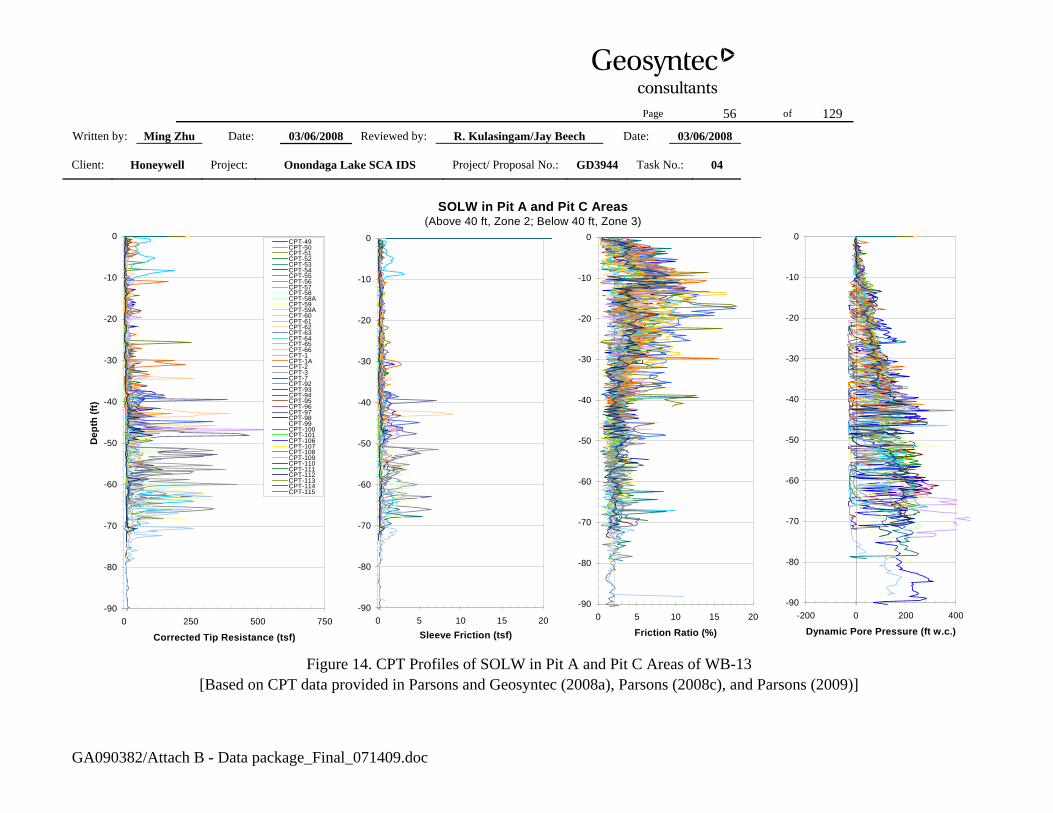
Page 56 of 129
Written by: Ming Zhu Date: 03/06/2008 Reviewed by: R. Kulasingam/Jay Beech Date: 03/06/2008
Client: Honeywell Project: Onondaga Lake SCA IDS Project/ Proposal No.: GD3944 Task No.: 04
GA090382/Attach B - Data package_Final_071409.doc
SOLW in Pit A and Pit C Areas(Above 40 ft, Zone 2; Below 40 ft, Zone 3)
-90
-80
-70
-60
-50
-40
-30
-20
-10
0
0 250 500 750
Corrected Tip Resistance (tsf)
Dep
th (f
t)
CPT-49CPT-50CPT-51CPT-52CPT-53CPT-54CPT-55CPT-56CPT-57CPT-58CPT-58ACPT-59CPT-59ACPT-60CPT-61CPT-62CPT-63CPT-64CPT-65CPT-66CPT-1CPT-1ACPT-2CPT-3CPT-7CPT-92CPT-93CPT-94CPT-95CPT-96CPT-97CPT-98CPT-99CPT-100CPT-101CPT-106CPT-107CPT-108CPT-109CPT-110CPT-111CPT-112CPT-113CPT-114CPT-115
-90
-80
-70
-60
-50
-40
-30
-20
-10
0
0 5 10 15 20Sleeve Friction (tsf)
-90
-80
-70
-60
-50
-40
-30
-20
-10
0
0 5 10 15 20
Friction Ratio (%)
-90
-80
-70
-60
-50
-40
-30
-20
-10
0
-200 0 200 400
Dynamic Pore Pressure (ft w.c.)
Figure 14. CPT Profiles of SOLW in Pit A and Pit C Areas of WB-13
[Based on CPT data provided in Parsons and Geosyntec (2008a), Parsons (2008c), and Parsons (2009)]

Page 57 of 129
Written by: Ming Zhu Date: 03/06/2008 Reviewed by: R. Kulasingam/Jay Beech Date: 03/06/2008
Client: Honeywell Project: Onondaga Lake SCA IDS Project/ Proposal No.: GD3944 Task No.: 04
GA090382/Attach B - Data package_Final_071409.doc
SOLW in "Pit D"
0
10
20
30
40
50
60
70
80
90
0 10 20 30 40SPT N Value
Dep
th (f
t)
SB915-PZ13-03
SB915-PZ13-04
SB915-PZ13-06
SB915-SB13-10
SB915-SB13-11
SB915-SB13-12
SOLW Near Dike
0
10
20
30
40
50
60
70
80
90
0 20 40 60 80SPT N Value
Dep
th (f
t)
SB915-PZ13-05SB915-PZ13-07SB915-PZ13-13SB915-SB13-01SB915-SB13-06SB915-SB13-08SB915-SB13-09SB915-SB13-13SB915-PZ13-02
SOLW in "Pit A" and "Pit C"
0
10
20
30
40
50
60
70
80
90
0 10 20 30 40SPT N Value
SB915-PZ13-01
SB915-SB13-02
SB915-SB13-03
SB915-SB13-04A
SB915-SB13-05
SB915-SB13-07
SB915-INEX-A7
SB915-INEX-A3 (Native)
SB915-INEX-A13
Figure 15. SPT N Value Profiles of SOLW at Selected Locations in WB-13
(Above 40 ft, Zone 2; Below 40 ft, Zone 3) (Zone 2) (Zone 1)

Page 58 of 129
Written by: Ming Zhu Date: 03/06/2008 Reviewed by: R. Kulasingam/Jay Beech Date: 03/06/2008
Client: Honeywell Project: Onondaga Lake SCA IDS Project/ Proposal No.: GD3944 Task No.: 04
GA090382/Attach B - Data package_Final_071409.doc
0
10
20
30
40
50
60
70
80
90
0 10 20 30 40 50 60 70 80
SPT N Value
Dep
th (f
t)
SOLW -- Zone 1
SOLW -- Zone 2
SOLW -- Zone 3
Range Average StandardDeviation
Zone 1 0 - 74 17 16Zone 2 0 - 18 1 2Zone 3 0 - 68 8 11
MaterialSPT Blow Counts (N)
SOLW
Figure 16. SPT N Value Versus Depth of SOLW
[based on boring logs presented in Parsons and Geosyntec (2008a), Parsons (2008c), and Parsons (2009)]

Page 59 of 129
Written by: Ming Zhu Date: 03/06/2008 Reviewed by: R. Kulasingam/Jay Beech Date: 03/06/2008
Client: Honeywell Project: Onondaga Lake SCA IDS Project/ Proposal No.: GD3944 Task No.: 04
GA090382/Attach B - Data package_Final_071409.doc
0
10
20
30
40
50
60
70
80
0 20 40 60 80 100 120SPT N Value
Dep
th (f
t)
SB915-PZ13-14SB915-PZ13-15SB915-PZ13-16SB915-SB13-28SB915-SB13-29SB915-SB13-30SB915-SB13-31
Gravel
SOLW
Gravel/Sand/Silt
Figure 17. SPT N Values from Borings in Inter-cell Dike between WB-13 and Wastebeds 12 and 14
[based on boring logs presented in Parsons (2008c) and Parsons (2009)]

Page 60 of 129
Written by: Ming Zhu Date: 03/06/2008 Reviewed by: R. Kulasingam/Jay Beech Date: 03/06/2008
Client: Honeywell Project: Onondaga Lake SCA IDS Project/ Proposal No.: GD3944 Task No.: 04
GA090382/Attach B - Data package_Final_071409.doc
0
20
40
60
80
100
120
140
160
0 20 40 60 80 100 120 140 160 180 200
SPT N Value
Dep
th (f
t)
Dike Soil
Foundation Soil Under Dike
Foundation Soil Under SOLW
Range Average StandardDeviation
5 - 127 36 222 - 120 40 23Foundation Soil
MaterialSPT Blow Counts (N)
Dike Soil
Figure 18. SPT N Values for Dike Soil and Foundation Soil
[based on boring logs presented in Parsons and Geosyntec (2008a), Parsons (2008c), Parsons (2009)]

Page 61 of 129
Written by: Ming Zhu Date: 03/06/2008 Reviewed by: R. Kulasingam/Jay Beech Date: 03/06/2008
Client: Honeywell Project: Onondaga Lake SCA IDS Project/ Proposal No.: GD3944 Task No.: 04
GA090382/Attach B - Data package_Final_071409.doc
Figure 19. Locations of Piezometers Monitored Since November 2006
Locations of monitored piezometers in circles

Page 62 of 129
Written by: Ming Zhu Date: 03/06/2008 Reviewed by: R. Kulasingam/Jay Beech Date: 03/06/2008
Client: Honeywell Project: Onondaga Lake SCA IDS Project/ Proposal No.: GD3944 Task No.: 04
GA090382/Attach B - Data package_Final_071409.doc
370.0
380.0
390.0
400.0
410.0
420.0
430.0
300.00320.00340.00360.00380.00400.00420.00440.00
Piezometer Tip Elevation (ft)
Ave
rage
GW
T El
evat
ion
(ft)
Piezometers Screened in SOLWPiezometers Screened in Natural Soil
SB915-PZ13-05N
SB915-PZ13-06N
SB915-PZ13-01NSB915-PZ13-10
SB915-PZ13-04N
SB915-PZ13-02N
Figure 20. Average GWT Elevation vs. Piezometer Tip Elevation

Page 63 of 129
Written by: Ming Zhu Date: 03/06/2008 Reviewed by: R. Kulasingam/Jay Beech Date: 03/06/2008
Client: Honeywell Project: Onondaga Lake SCA IDS Project/ Proposal No.: GD3944 Task No.: 04
GA090382/Attach B - Data package_Final_071409.doc
Figure 21. Locations of Cross Sections Showing Measured Groundwater Table Elevations

Page 64 of 129
Written by: Ming Zhu Date: 03/06/2008 Reviewed by: R. Kulasingam/Jay Beech Date: 03/06/2008
Client: Honeywell Project: Onondaga Lake SCA IDS Project/ Proposal No.: GD3944 Task No.: 04
GA090382/Attach B - Data package_Final_071409.doc
Figure 22. Measured Groundwater Table Elevations on Cross Section 1

Page 65 of 129
Written by: Ming Zhu Date: 03/06/2008 Reviewed by: R. Kulasingam/Jay Beech Date: 03/06/2008
Client: Honeywell Project: Onondaga Lake SCA IDS Project/ Proposal No.: GD3944 Task No.: 04
GA090382/Attach B - Data package_Final_071409.doc
Figure 23. Measured Groundwater Table Elevations on Cross Section 2

Page 66 of 129
Written by: Ming Zhu Date: 03/06/2008 Reviewed by: R. Kulasingam/Jay Beech Date: 03/06/2008
Client: Honeywell Project: Onondaga Lake SCA IDS Project/ Proposal No.: GD3944 Task No.: 04
GA090382/Attach B - Data package_Final_071409.doc
0
10
20
30
40
50
60
70
80
0 100 200 300 400 500 600 700 800 900 1000
Water Content (%)
Dep
th (f
t)
SOLW -- Zone 1SOLW -- Zone 2SOLW -- Zone 3
0
5
10
15
20
25
30
35
40
45
50
0 50 100
150
200
250
300
350
400
450
500
550
600
650
700
750
800
850
900
More
Water Content of SOLW (%)
Freq
uenc
y
Note: Data include the water contents measured from index property tests, UU tests, and CU tests during the 2004, Phase I, Phase II, and Phase III investigations.
SOLW (all 3 zones)
Range Average StandardDeviation
Zone 1 64 - 367 166 80Zone 2 10 - 912 227 103Zone 3 5 - 294 172 63
All 3 Zones 5 - 912 212 99
Water Content (%)
SOLW
Material
Figure 24. Water Content of SOLW
[Data from the summary tables provided in Attachment 3]

Page 67 of 129
Written by: Ming Zhu Date: 03/06/2008 Reviewed by: R. Kulasingam/Jay Beech Date: 03/06/2008
Client: Honeywell Project: Onondaga Lake SCA IDS Project/ Proposal No.: GD3944 Task No.: 04
GA090382/Attach B - Data package_Final_071409.doc
0.0
10.0
20.0
30.0
40.0
50.0
60.0
70.0
80.0
0.0 50.0 100.0 150.0 200.0 250.0 300.0 350.0 400.0
Water Content (%)
Dep
th (f
t)
Dike Soil
Foundation Soil
SOLW Underneath Inter-Cell Dikes
Notes:(1). Data include the water contents measured from index property tests, UU tests, and CU tests during the 2004, Phase I, Phase II, and Phase III investigations. (2). SOLW encountered underneath the inter-cell dikes between WB-13, WB12 and WB-14 were not considered in calculating the range, average value, and the standard deviation of the dike soil.
Range Average StandardDeviation
3 - 83 13 104 - 66 16 12
MaterialWater Content (%)
Dike SoilFoundation Soil
Figure 25. Water Content of Dike Soil and Foundation Soil [Data from the summary tables provided in Attachment 3]

Page 68 of 129
Written by: Ming Zhu Date: 03/06/2008 Reviewed by: R. Kulasingam/Jay Beech Date: 03/06/2008
Client: Honeywell Project: Onondaga Lake SCA IDS Project/ Proposal No.: GD3944 Task No.: 04
GA090382/Attach B - Data package_Final_071409.doc
0
10
20
30
40
50
60
70
80
0 50 100 150 200 250
Plasticity Index
Dep
th (f
t)
SOLW -- Zone 1SOLW -- Zone 2SOLW -- Zone 3
Note: Data include results of index property tests during the 2004, Phase I, Phase II, and Phase III investigations.
Range Average StandardDeviation
Zone 1 12 -74 36 16Zone 2 27 - 127 55 20Zone 3 22 - 138 69 41
All 3 Zones 12 - 138 53 26
Material
SOLW
Plasticity Index
Figure 26. Plasticity Index of SOLW
[Data from the summary tables provided in Attachment 3]

Page 69 of 129
Written by: Ming Zhu Date: 03/06/2008 Reviewed by: R. Kulasingam/Jay Beech Date: 03/06/2008
Client: Honeywell Project: Onondaga Lake SCA IDS Project/ Proposal No.: GD3944 Task No.: 04
GA090382/Attach B - Data package_Final_071409.doc
0
10
20
30
40
50
60
70
80
0 10 20 30 40 50 60 70 80
Plasticity Index
Dep
th (f
t)
Dike Soil
Foundation Soil
SOLW Underneath Inter-Cell Dikes
Notes:(1). Data include results of index property tests during the 2004, Phase I, Phase II, and Phase III investigations.(2). SOLW encountered underneath the inter-cell dike between WB-13 and WB-14 were not considered in calculating the range, average value, and the standard deviation of the dike soil.
Range Average StandardDeviation
6 - 17 10 33 - 30 11 7
MaterialPlasticity Index
Dike SoilFoundation Soil
Figure 27. Plasticity Index of Dike Soil and Foundation Soil [Data from the summary tables provided in Attachment 3]

Page 70 of 129
Written by: Ming Zhu Date: 03/06/2008 Reviewed by: R. Kulasingam/Jay Beech Date: 03/06/2008
Client: Honeywell Project: Onondaga Lake SCA IDS Project/ Proposal No.: GD3944 Task No.: 04
GA090382/Attach B - Data package_Final_071409.doc
0
10
20
30
40
50
60
70
80
50 70 90 110 130 150 170 190 210
Total Unit Weight (pcf)
Dep
th (f
t)
SOLW -- Zone 1
SOLW -- Zone 2
SOLW -- Zone 3
Foundation Soil
0
5
10
15
20
25
30
35
50 55 60 65 70 75 80 85 90 95 100
105
110
115
120
125
130
135
140
145
150
More
Total Unit Wight of SOLW (pcf)
Freq
uenc
y
Note: Data include the unit weights measured from index property tests, UU tests, and CU tests during the 2004, Phase I, Phase II, and Phase III investigations.
SOLW (all 3 zones)
Foundation Soil Range Average StandardDeviation
Zone 1 69 - 108 84 10Zone 2 55 - 139 82 13Zone 3 68 - 101 82 8
All 3 Zones 55 - 139 82 12118 - 124 121 3
SOLW
Soil
Foundation Soil
Total Unit Weight (pcf)
Figure 28. Total Unit Weight of SOLW and Foundation Soil [Data from the summary tables provided in Attachment 3]
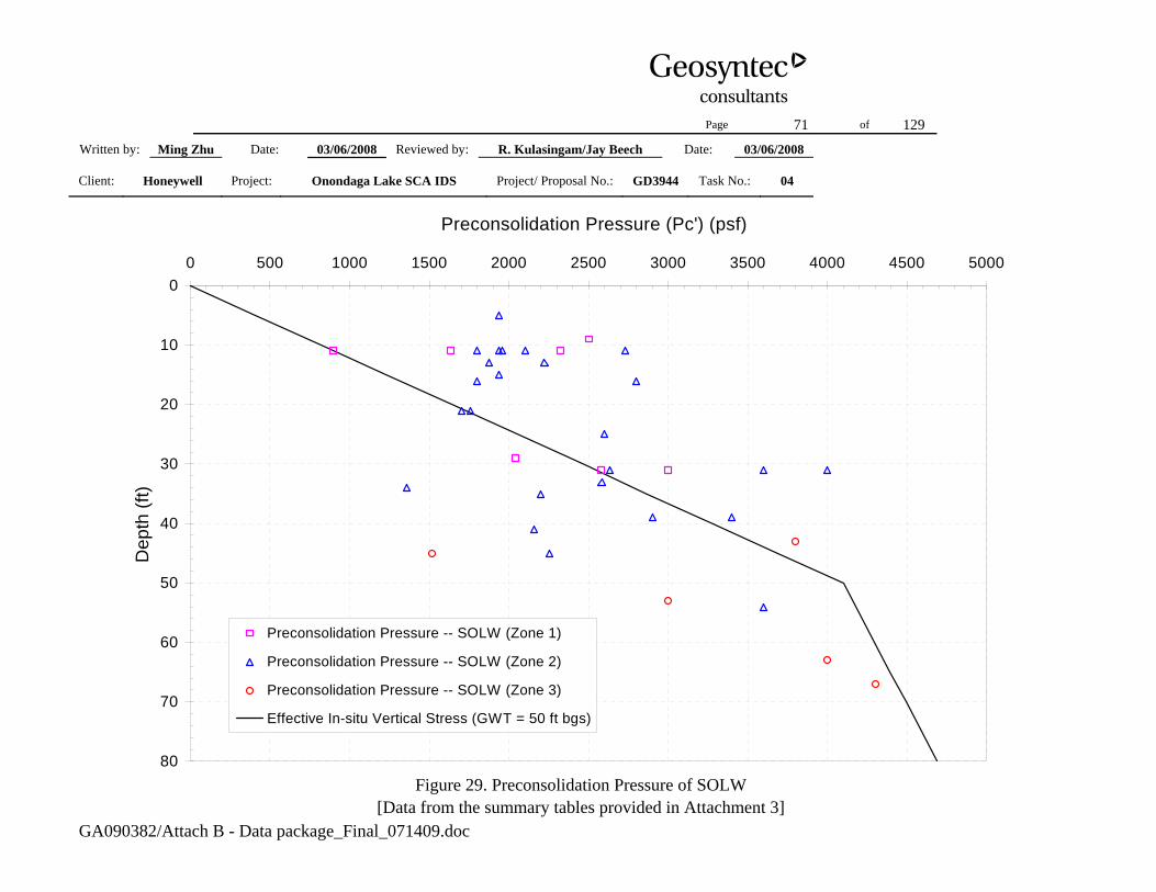
Page 71 of 129
Written by: Ming Zhu Date: 03/06/2008 Reviewed by: R. Kulasingam/Jay Beech Date: 03/06/2008
Client: Honeywell Project: Onondaga Lake SCA IDS Project/ Proposal No.: GD3944 Task No.: 04
GA090382/Attach B - Data package_Final_071409.doc
0
10
20
30
40
50
60
70
80
0 500 1000 1500 2000 2500 3000 3500 4000 4500 5000
Preconsolidation Pressure (Pc') (psf)
Dep
th (f
t)
Preconsolidation Pressure -- SOLW (Zone 1)
Preconsolidation Pressure -- SOLW (Zone 2)
Preconsolidation Pressure -- SOLW (Zone 3)
Effective In-situ Vertical Stress (GWT = 50 ft bgs)
Figure 29. Preconsolidation Pressure of SOLW
[Data from the summary tables provided in Attachment 3]

Page 72 of 129
Written by: Ming Zhu Date: 03/06/2008 Reviewed by: R. Kulasingam/Jay Beech Date: 03/06/2008
Client: Honeywell Project: Onondaga Lake SCA IDS Project/ Proposal No.: GD3944 Task No.: 04
GA090382/Attach B - Data package_Final_071409.doc
0
10
20
30
40
50
60
70
80
0 1 2 3 4 5 6
Overconsolidation Ratio (OCR)
Dep
th (f
t)
SOLW -- Zone 1SOLW -- Zone 2SOLW -- Zone 3OCR for Design
Recommended OCR for design: OCR = 4.5, for D = 0~10 ft OCR = 2.0, for D = 10~20 ft OCR = 1.0, for D > 20 ft
Figure 30. Overconsolidation Ratio of SOLW

Page 73 of 129
Written by: Ming Zhu Date: 03/06/2008 Reviewed by: R. Kulasingam/Jay Beech Date: 03/06/2008
Client: Honeywell Project: Onondaga Lake SCA IDS Project/ Proposal No.: GD3944 Task No.: 04
GA090382/Attach B - Data package_Final_071409.doc
0
10
20
30
40
50
60
70
80
0.00 0.10 0.20 0.30 0.40 0.50 0.60 0.70 0.80 0.90 1.00Modified Compression Index (Ccε)
Dep
th (f
t)
SOLW Zone 1 (Phase II Lab Tests)
SOLW Zone 2 (Phase II Lab Tests)SOLW Zone 2 (Phase I Lab Tests)
SOLW Zone 2 (2004 Lab Tests)SOLW Zone 3 (Phase III Lab Tests)
SOLW Zone 3 (2004 Lab Tests)
Number of tests Range AveragePhase III Lab Tests Zone 3 4 0.34~0.46 0.38
Zone 1 7 0.15~0.50 0.34Zone 2 14 0.27~0.71 0.47
Phase I Lab Tests Zone 2 6 0.40~0.61 0.50
Zone 2 5 0.21~0.65 0.37Zone 3 1 0.21 0.21
Phase II Lab Tests
Summary of Ccε
2004 Lab Tests
Number of tests Range AverageZone 1 7 0.15~0.50 0.34Zone 2 25 0.21~0.71 0.46Zone 3 5 0.21~0.46 0.38
SOLW Summary of Ccε
Figure 31. Modified Compression Index of SOLW
[Data from the summary tables provided in Attachment 3]

Page 74 of 129
Written by: Ming Zhu Date: 03/06/2008 Reviewed by: R. Kulasingam/Jay Beech Date: 03/06/2008
Client: Honeywell Project: Onondaga Lake SCA IDS Project/ Proposal No.: GD3944 Task No.: 04
GA090382/Attach B - Data package_Final_071409.doc
0
10
20
30
40
50
60
70
80
0.000 0.010 0.020 0.030 0.040 0.050 0.060 0.070
Modified Recompression Index (Crε)
Dep
th (f
t)
SOLW -- Zone 1 (Phase II Lab Tests)
SOLW -- Zone 2 (Phase II Lab Tests)
SOLW -- Zone 2 (Phase I Lab Tests)
SOLW -- Zone 2 (2004 Lab Tests)
SOLW -- Zone 3 (Phase III Lab Tests)
SOLW -- Zone 3 (2004 Lab Tests)
Number of tests Range AveragePhase III Lab Tests Zone 3 4 0.015~0.034 0.021
Zone 1 7 0.010~0.020 0.015Zone 2 14 0.011~0.025 0.018
Phase I Lab Tests Zone 2 6 0.004~0.010 0.007
Zone 2 5 0.005~0.018 0.010Zone 3 1 0.003 0.003
Summary of Crε
2004 Lab Tests
Phase II Lab Tests
Number of tests Range AverageZone 1 7 0.010~0.020 0.015Zone 2 25 0.004~0.025 0.014Zone 3 5 0.003~0.034 0.021
Summary of CrεSOLW
Figure 32. Modified Recompression Index of SOLW
[Data from the summary tables provided in Attachment 3]

Page 75 of 129
Written by: Ming Zhu Date: 03/06/2008 Reviewed by: R. Kulasingam/Jay Beech Date: 03/06/2008
Client: Honeywell Project: Onondaga Lake SCA IDS Project/ Proposal No.: GD3944 Task No.: 04
GA090382/Attach B - Data package_Final_071409.doc
0.00%
0.50%
1.00%
1.50%
2.00%
2.50%
0.01 0.1 1 10 100Stress Ratio (σ'v/p'c)
Mod
ified
Sec
onda
ry C
ompr
essi
on In
dex
(Cα
ε)
PZ13-02/0295-06/C-24 (Depth = 10-12 ft)SB13-01/0297-05/C-19 (Depth = 28-30 ft)SB13-06/0298-12/C-9 (Depth = 8-10 ft)SB13-06/0298-14/C-7 (Depth = 30-32 ft)SB13-09/0299-07/C-11 (Depth = 10-12 ft)SB13-09/0299-09/C-2 (Depth = 30-32 ft)SB13-13/0300-12/C-17 (Depth = 10-12 ft)For Design
SOLW (Zone 1)
Cαε = 0.13%, for σv'/Pc' <= 1.0Cαε = 0.83%, for σv'/Pc' > 1.0
Figure 33. Modified Secondary Compression Index for SOLW in Zone 1
[based on 1-D consolidation test reports provided in Parsons and Geosyntec (2008a) and Parsons (2008c)]

Page 76 of 129
Written by: Ming Zhu Date: 03/06/2008 Reviewed by: R. Kulasingam/Jay Beech Date: 03/06/2008
Client: Honeywell Project: Onondaga Lake SCA IDS Project/ Proposal No.: GD3944 Task No.: 04
GA090382/Attach B - Data package_Final_071409.doc
0.00%
0.50%
1.00%
1.50%
2.00%
2.50%
0.01 0.1 1 10 100
Stress Ratio (σ'v/p'c)
Mod
ified
Sec
onda
ry C
ompr
essi
on In
dex
(Cα
ε)
6001-01/A-2/C-9 (Depth = 10-12 ft)6000-10/A-2/C-1 (Depth = 34-36 ft)6001-04/A-2/C-8 (Depth = 38-40 ft)6000-02/A-7/C-3 (Depth = 15-17 ft)6000-02/A-7/C-4 (Depth = 15-17 ft)6000-07/A-10/C-2 (Depth = 24-26 ft)PZ13-03/0295-11/C-6 (Depth = 10-12 ft)PZ13-03/0295-13/C-20 (Depth = 30-32 ft)PZ13-04/0295-17/C-12 (Depth = 10-12 ft)PZ13-04/0295-19/C-21 (Depth = 33-35 ft)SB13-03/0297-13/C-4 (Depth = 4-6 ft)SB13-03/0297-15/C123 (Depth = 32-34 ft)SB13-04A/0297-18/C-15 (Depth = 12-14 ft)SB13-04A/0297-20/C-13 (Depth = 38-40 ft)SB13-05/0298-04/C-3 (Depth = 14-16 ft)SB13-05/0298-07/C-1A (Depth = 30-32 ft)SB13-12/0300-08/C-25 (Depth = 12-14 ft)SB13-12/0300-09/C-5A (Depth = 30-32 ft)SB13-12/0300-11/C-23 (Depth = 44-46 ft)PZ-02 (Depth = 20-22 ft)PZ-02 (Depth = 40-42 ft)SB-21 (Depth = 10-12 ft)SB-22 (Depth = 20-22 ft)PZ-01 (Depth = 10-12 ft)For Design
SOLW (Zone 2)
Cαε = 0.11%, for σv'/Pc' <= 1.0Cαε = 0.91%, for σv'/Pc' > 1.0
Figure 34. Modified Secondary Compression Index for SOLW in Zone 2
[based on 1-D consolidation test reports provided in Parsons and Geosyntec (2008a) and Parsons (2008c)]

Page 77 of 129
Written by: Ming Zhu Date: 03/06/2008 Reviewed by: R. Kulasingam/Jay Beech Date: 03/06/2008
Client: Honeywell Project: Onondaga Lake SCA IDS Project/ Proposal No.: GD3944 Task No.: 04
GA090382/Attach B - Data package_Final_071409.doc
0.00%
0.50%
1.00%
1.50%
2.00%
2.50%
0.01 0.1 1 10 100
Stress Ratio (σ'v/p'c)
Mod
ified
Sec
onda
ry C
ompr
essi
on In
dex
(Cα
ε)
PZ-01 (Depth = 44-46 ft)SB13-14/0465-04/C-1A (Depth = 62-64 ft)SB13-15/0465-08/C-4 (Depth = 42-44 ft)SB13-16/0465-16/C-3SB13-17/0465-22/C-2For Design
SOLW (Zone 3)
Cαε = 0.07%, for σv'/Pc' <= 1.0Cαε = 0.70%, for σv'/Pc' > 1.0
Figure 35. Modified Secondary Compression Index for SOLW in Zone 3
[based on 1-D consolidation test reports provided in Parsons and Geosyntec (2008a), Parsons (2008c;2009)]

Page 78 of 129
Written by: Ming Zhu Date: 03/06/2008 Reviewed by: R. Kulasingam/Jay Beech Date: 03/06/2008
Client: Honeywell Project: Onondaga Lake SCA IDS Project/ Proposal No.: GD3944 Task No.: 04
GA090382/Attach B - Data package_Final_071409.doc
0
0.05
0.1
0.15
0.2
0.25
0.3
0.01 0.1 1 10 100
Stress Ratio (σ'v/p'c)
Coe
ffici
ent o
f Con
solid
aton
(Cv)
(cm
2 /s)
PZ13-02/0295-06/C-24 (Depth = 10-12 ft)SB13-01/0297-05/C-19 (Depth = 28-30 ft)SB13-06/0298-12/C-9 (Depth = 8-10 ft)SB13-06/0298-14/C-7 (Depth = 30-32 ft)SB13-09/0299-07/C-11 (Depth = 10-12 ft)SB13-09/0299-09/C-2 (Depth = 30-32 ft)SB13-13/0300-12/C-17 (Depth = 10-12 ft)For Design
SOLW (Zone 1)
Cv = 0.047 cm2/s, for σv'/Pc' <= 1.0Cv = 0.029 cm2/s, for σv'/Pc' > 1.0
Figure 36. Coefficient of Consolidation for SOLW in Zone 1
[based on 1-D consolidation test reports provided in Parsons and Geosyntec (2008a) and Parsons (2008c)]
Note: Seven data points above the dashed-line boxes were not used to calculate the average value.

Page 79 of 129
Written by: Ming Zhu Date: 03/06/2008 Reviewed by: R. Kulasingam/Jay Beech Date: 03/06/2008
Client: Honeywell Project: Onondaga Lake SCA IDS Project/ Proposal No.: GD3944 Task No.: 04
GA090382/Attach B - Data package_Final_071409.doc
0
0.05
0.1
0.15
0.2
0.25
0.3
0.01 0.1 1 10 100
Stress Ratio (σ'v/p'c)
Coe
ffici
ent o
f Con
solid
aton
(Cv)
(cm
2 /s)
6001-01/A-2/C-9 (Depth = 10-12 ft)6000-10/A-2/C-1 (Depth = 34-36 ft)6001-04/A-2/C-8 (Depth = 38-40 ft)6000-02/A-7/C-3 (Depth = 15-17 ft)6000-02/A-7/C-4 (Depth = 15-17 ft)6000-07/A-10/C-2 (Depth = 24-26 ft)PZ13-03/0295-11/C-6 (Depth = 10-12 ft)PZ13-03/0295-13/C-20 (Depth = 30-32 ft)PZ13-04/0295-17/C-12 (Depth = 10-12 ft)PZ13-04/0295-19/C-21 (Depth = 33-35 ft)SB13-03/0297-13/C-4 (Depth = 4-6 ft)SB13-03/0297-15/C123 (Depth = 32-34 ft)SB13-04A/0297-18/C-15 (Depth = 12-14 ft)SB13-04A/0297-20/C-13 (Depth = 38-40 ft)SB13-05/0298-04/C-3 (Depth = 14-16 ft)SB13-05/0298-07/C-1A (Depth = 30-32 ft)SB13-12/0300-08/C-25 (Depth = 12-14 ft)SB13-12/0300-09/C-5A (Depth = 30-32 ft)SB13-12/0300-11/C-23 (Depth = 44-46 ft)PZ-01 (Depth = 10-12 ft)PZ-02 (Depth = 20-22 ft)PZ-02 (Depth = 40-42 ft)SB-21 (Depth = 10-12 ft)SB-22 (Depth = 20-22 ft)For Design
SOLW (Zone 2)
Cv = 0.046 cm2/s, for σv'/Pc' <= 1.0Cv = 0.009 cm2/s, for σv'/Pc' > 1.0
Figure 37. Coefficient of Consolidation for SOLW in Zone 2
[based on 1-D consolidation test reports provided in Parsons and Geosyntec (2008a) and Parsons (2008c)]
Note: Three data points above the dashed-line boxes were not used to calculate the average

Page 80 of 129
Written by: Ming Zhu Date: 03/06/2008 Reviewed by: R. Kulasingam/Jay Beech Date: 03/06/2008
Client: Honeywell Project: Onondaga Lake SCA IDS Project/ Proposal No.: GD3944 Task No.: 04
GA090382/Attach B - Data package_Final_071409.doc
0
0.05
0.1
0.15
0.2
0.25
0.3
0.01 0.1 1 10 100
Stress Ratio (σ'v/p'c)
Coe
ffici
ent o
f Con
solid
aton
(Cv)
(cm
2 /s)
PZ-01 (Depth = 44-46 ft)SB13-14/0465-04/C-1A (Depth = 62-64 ft)SB13-15/0465-08/C-4 (Depth = 42-44 ft)SB13-16/0465-16/C-3SBSB13-17/0465-22/C-2For Design
SOLW (Zone 3)
Cv = 0.024 cm2/s, for σv'/Pc' <= 1.0Cv = 0.008 cm2/s, for σv'/Pc' > 1.0
Figure 38. Coefficient of Consolidation for SOLW in Zone 3
[based on 1-D consolidation test reports provided in Parsons and Geosyntec (2008a) and Parsons (2008c;2009)]

Page 81 of 129
Written by: Ming Zhu Date: 03/06/2008 Reviewed by: R. Kulasingam/Jay Beech Date: 03/06/2008
Client: Honeywell Project: Onondaga Lake SCA IDS Project/ Proposal No.: GD3944 Task No.: 04
GA090382/Attach B - Data package_Final_071409.doc
0.00
0.10
0.20
0.30
0.40
0.50
0.60
0.70
0.80
0.90
0 20 40 60 80 100 120
Time (days)
Coe
ffici
ent o
f Con
solid
atio
n (C
v) (c
m2 /s
)
A-1A-2A-3A-4A-5A-6A-7A-8A-9A-10A-11
Figure 39. Coefficient of Consolidation from Phase I Pilot Study

Page 82 of 129
Written by: Ming Zhu Date: 03/06/2008 Reviewed by: R. Kulasingam/Jay Beech Date: 03/06/2008
Client: Honeywell Project: Onondaga Lake SCA IDS Project/ Proposal No.: GD3944 Task No.: 04
GA090382/Attach B - Data package_Final_071409.doc
0.00
0.10
0.20
0.30
0.40
0.50
0.60
0.70
0.80
0.90
1.00
1.10
1.20
1.30
1.40
1.50
1.60
0 2000 4000 6000 8000 10000 12000 14000
σ3' (psf)
Su/ σ
3'
SOLW -- Zone 1 (Phase II Lab Tests)
SOLW -- Zone 2 (Phase II Lab Tests)
SOLW -- Zone 2 (Phase I Lab Tests)
SOLW -- Zone 2 (2004 Lab Tests)
SOLW -- Zone 3 (Phase II Lab Tests)
SOLW -- Zone 3 (2004 Lab Tests)
Figure 40. Undrained Strength Ratio of SOLW
[Data from the summary tables provided in Attachment 3]

Page 83 of 129
Written by: Ming Zhu Date: 03/06/2008 Reviewed by: R. Kulasingam/Jay Beech Date: 03/06/2008
Client: Honeywell Project: Onondaga Lake SCA IDS Project/ Proposal No.: GD3944 Task No.: 04
GA090382/Attach B - Data package_Final_071409.doc
0
10
20
30
40
50
60
70
80
0 1000 2000 3000 4000 5000 6000
Undrained Shear Strength (Su) (psf)
Dep
th (f
t)
SOLW -- Zone 1 (Phase II Lab Tests)SOLW -- Zone 2 (Phase II Lab Tests)SOLW -- Zone 2 (Phase I Lab Tests)SOLW -- Zone 2 (2004 Lab Tests)SOLW -- Zone 3 (Phase II Lab Tests)SOLW -- Zone 3 (2004 Lab Tests)Correlation: Su=0.3OCR^0.8Sv'For Design
Note: (1). Outlying data points that are greater than 2000 psf were not considered in calculation of the average Su of SOLW.(2). Discontinuity of Su from the empirical correlation is due to the changes of OCR at 10 ft and 20 ft, and the water table at 50 ft.
Range Average Range Average Range Average0 - 20 ft 444 - 767 592 527 - 748 63320 - 40 ft 916 - 1431 1113 419 - 1353 780
>40 ft 719 719 320 - 1479 899
Depth
N/A
N/AN/A
Su of SOLW (psf)Zone 1 Zone 2 Zone 3
Figure 41. Undrained Shear Strength of SOLW
[Data from the summary tables provided in Attachment 3]

Page 84 of 129
Written by: Ming Zhu Date: 03/06/2008 Reviewed by: R. Kulasingam/Jay Beech Date: 03/06/2008
Client: Honeywell Project: Onondaga Lake SCA IDS Project/ Proposal No.: GD3944 Task No.: 04
GA090382/Attach B - Data package_Final_071409.doc
0
5
10
15
20
25
30
35
40
45
50
0 5 10 15 20 25 30 35 40 45 50
Settlement Measured on January 10, 2008 (inches)
Prim
ary
Set
tlem
ent P
redi
cted
U
sing
Lab
Dat
a (in
ches
)
A-1A-2A-3A-4A-5A-6A-7A-9A-11A-8A-10
Point 3
Point 4
Point 2Point 1
Figure 42. Comparison of Predicted Settlement with Settlement from Phase I Pilot Study

Page 85 of 129
Written by: Ming Zhu Date: 03/06/2008 Reviewed by: R. Kulasingam/Jay Beech Date: 03/06/2008
Client: Honeywell Project: Onondaga Lake SCA IDS Project/ Proposal No.: GD3944 Task No.: 04
GA090382/Attach B - Data package_Final_071409.doc
0
10
20
30
40
50
0.00 100.00 200.00 300.00 400.00 500.00 600.00 700.00 800.00 900.00
Time (days)
Set
tlem
ent (
inch
)
Field Monitoring at A-1
Field Monitoring at A-2
Prediction at Point 1
Figure 43. Prediction of Time Rate of Consolidation at Point 1

Page 86 of 129
Written by: Ming Zhu Date: 03/06/2008 Reviewed by: R. Kulasingam/Jay Beech Date: 03/06/2008
Client: Honeywell Project: Onondaga Lake SCA IDS Project/ Proposal No.: GD3944 Task No.: 04
GA090382/Attach B - Data package_Final_071409.doc
0
10
20
30
40
50
0.00 100.00 200.00 300.00 400.00 500.00 600.00 700.00 800.00 900.00
Time (days)
Set
tlem
ent (
inch
)
Field Monitoring at A-3Field Monitoring at A-4Field Monitoring at A-5Field Monitoring at A-6Prediction at Point 2
Figure 44. Prediction of Time Rate of Consolidation at Point 2

Page 87 of 129
Written by: Ming Zhu Date: 03/06/2008 Reviewed by: R. Kulasingam/Jay Beech Date: 03/06/2008
Client: Honeywell Project: Onondaga Lake SCA IDS Project/ Proposal No.: GD3944 Task No.: 04
GA090382/Attach B - Data package_Final_071409.doc
0
10
20
30
40
50
0.00 100.00 200.00 300.00 400.00 500.00 600.00 700.00 800.00 900.00
Time (days)
Set
tlem
ent (
inch
)
Field Monitoring at A-7
Field Monitoring at A-9
Field Monitoring at A-11
Prediction at Point 3
Figure 45. Prediction of Time Rate of Consolidation at Point 3

Page 88 of 129
Written by: Ming Zhu Date: 03/06/2008 Reviewed by: R. Kulasingam/Jay Beech Date: 03/06/2008
Client: Honeywell Project: Onondaga Lake SCA IDS Project/ Proposal No.: GD3944 Task No.: 04
GA090382/Attach B - Data package_Final_071409.doc
0
10
20
30
40
50
0.00 100.00 200.00 300.00 400.00 500.00 600.00 700.00 800.00 900.00
Time (days)
Set
tlem
ent (
inch
)
Field Monitoring at A-8Field Monitoring at A-10Prediction at Point 4
Figure 46. Prediction of Time Rate of Consolidation at Point 4
Abnormal Data Point

Page 89 of 129
Written by: Ming Zhu Date: 03/06/2008 Reviewed by: R. Kulasingam/Jay Beech Date: 03/06/2008
Client: Honeywell Project: Onondaga Lake SCA IDS Project/ Proposal No.: GD3944 Task No.: 04
GA090382/Attach B - Data package_Final_071409.doc
Attachment 1
Estimated Solvay Waste Thickness
(Provided to Geosyntec by Parsons; Phase III Thicknesses were added by Geosyntec)

Page 90 of 129
Written by: Ming Zhu Date: 03/06/2008 Reviewed by: R. Kulasingam/Jay Beech Date: 03/06/2008
Client: Honeywell Project: Onondaga Lake SCA IDS Project/ Proposal No.: GD3944 Task No.: 04
GA090382/Attach B - Data package_Final_071409.doc
Attachment 2
Piezometer Data Collected Between November 2006 and December 2007
(Provided to Geosyntec by Parsons)

Page 91 of 129
Written by: Ming Zhu Date: 03/06/2008 Reviewed by: R. Kulasingam/Jay Beech Date: 03/06/2008
Client: Honeywell Project: Onondaga Lake SCA IDS Project/ Proposal No.: GD3944 Task No.: 04
GA090382/Attach B - Data package_Final_071409.doc
Attachment 3
Summary Tables of Lab Test Results

Page 92 of 129
Written by: Ming Zhu Date: 03/06/2008 Reviewed by: R. Kulasingam/Jay Beech Date: 03/06/2008
Client: Honeywell Project: Onondaga Lake SCA IDS Project/ Proposal No.: GD3944 Task No.: 04
GA090382/Attach B - Data package_Final_071409.doc
2004 Lab Results
(Presented in Appendix A of the report titled “Onondaga Lake Pre-Design Investigation: Wastebed 13 Settlement Pilot Study Data Summary Report” prepared by Parsons and Geosyntec
2008a)

Page 93 of 129
Written by: Ming Zhu Date: 03/06/2008 Reviewed by: R. Kulasingam/Jay Beech Date: 03/06/2008
Client: Honeywell Project: Onondaga Lake SCA IDS Project/ Proposal No.: GD3944 Task No.: 04
GA090382/Attach B - Data package_Final_071409.doc
Phase I Lab Results
(Presented in the report titled “Onondaga Lake Pre-Design Investigation: Wastebed 13 Settlement Pilot Study Data Summary Report, Onondaga County, New York” prepared by Parsons and Geosyntec
[2008a])

Page 94 of 129
Written by: Ming Zhu Date: 03/06/2008 Reviewed by: R. Kulasingam/Jay Beech Date: 03/06/2008
Client: Honeywell Project: Onondaga Lake SCA IDS Project/ Proposal No.: GD3944 Task No.: 04
GA090382/Attach B - Data package_Final_071409.doc
Phase II Lab Results
(Provided to Geosyntec by Parsons and included in the report “Onondaga Lake Pre-Design Investigation: Phase II Data Summary Report” prepared by Parsons [2008c])

Page 95 of 129
Written by: Ming Zhu Date: 03/06/2008 Reviewed by: R. Kulasingam/Jay Beech Date: 03/06/2008
Client: Honeywell Project: Onondaga Lake SCA IDS Project/ Proposal No.: GD3944 Task No.: 04
GA090382/Attach B - Data package_Final_071409.doc
Phase III Lab Results
(Provided to Geosyntec by Parsons and included in Appendix E of “Onondaga Lake Pre-Design Investigation Phase III Data Summary Report” prepared by Parsons in 2008)

Page 96 of 129
Written by: Ming Zhu Date: 03/06/2008 Reviewed by: R. Kulasingam/Jay Beech Date: 03/06/2008
Client: Honeywell Project: Onondaga Lake SCA IDS Project/ Proposal No.: GD3944 Task No.: 04
GA090382/Attach B - Data package_Final_071409.doc
Attachment 4
Verification of Subsurface Model and Compressibility of SOLW Based on Test Pad Results

Page 97 of 129
Written by: Ming Zhu Date: 03/06/2008 Reviewed by: R. Kulasingam/Jay Beech Date: 03/06/2008
Client: Honeywell Project: Onondaga Lake SCA IDS Project/ Proposal No.: GD3944 Task No.: 04
GA090382/Attach B - Data package_Final_071409.doc
Part I: Prediction of Primary Consolidation Settlement Based on Field Test Data
Introduction
Terzaghi’s one dimensional (1-D) consolidation theory was used to interpret the field test results from the Phase I Settlement Pilot Study and to predict the primary consolidation settlement. The initial excess pore water pressure was assumed to be constant throughout the SOLW layer and two-way drainage was assumed (i.e., at top and bottom of the waste). The average thickness of the SOLW layer under the test fill is calculated to be 72 ft. Hence, the longest drainage path drH is equal to one-half of the layer thickness (i.e., 36 ft). The major calculation steps included the following.
1. Use the excess pore water pressure measured in the field to develop the excess pore water pressure profile at each piezometer location for each time period that piezometers were monitored. The location of piezometers A-1 through A-11 are presented in Figure 4-1 of this attachment.
2. Use the excess pore water pressure profile at each piezometer to calculate the average degree of consolidation for the entire depth of the compressible SOLW layer at each monitoring time period.
3. Use the calculated average degree of consolidation for the SOLW layer at each monitoring time period to calculate the coefficient of consolidation.
4. Use the measured settlements and the calculated average degree of consolidation at each time period for each piezometer location to predict the primary consolidation settlement at that location.
Piezometer and settlement data that was recorded during the time period between October 15, 2005 and January 5, 2006 (i.e., approximately 100 days after the placement of test fill) was considered in prediction of the primary consolidation settlement. The predicted primary settlement is compared to field data measured on January 10, 2008 (i.e., approximately 2.3 years after the placement of test fill) in Part III of this attachment.
Calculation of Degree of consolidation
The degree of consolidation at any depth was calculated by
0
1),(uutzU z−=
where

Page 98 of 129
Written by: Ming Zhu Date: 03/06/2008 Reviewed by: R. Kulasingam/Jay Beech Date: 03/06/2008
Client: Honeywell Project: Onondaga Lake SCA IDS Project/ Proposal No.: GD3944 Task No.: 04
GA090382/Attach B - Data package_Final_071409.doc
zu = excess pore water pressure at any depth at a given time t.
0u = initial excess pore water pressure Measured excess pore water pressures were recorded in the field by Parsons as the equivalent water pressure (i.e., piezometric) head. Based on the fill loading process and the stress distribution below the test fill (see Part II of this attachment for discussion regarding stress distribution), the initial excess pore water pressure head used in subsequent analyses was assumed to be the measured excess pore water pressure after the end of fill placement. Based on the data provided by Parsons, these values were assumed to be: (i) 18 ft for locations A-1 through A-6; and (ii) 14.4 ft for locations A-7 through A-11. The typical piezometer response to loading that shows these initial excess pore water pressure heads after the end of fill placement as well as the excess pore water pressures at other monitoring periods is presented in Figure 4-2. Using these field monitoring results and the referenced equation, the degree of consolidation for each piezometer at selected monitoring time periods was calculated. Results from each piezometer location are presented in Figure 4-3. It is noted that rainfall and snowmelt in late December 2005 and early January 2006 combined to locally increase the water levels in most piezometers, resulting in a decrease in the calculated degree of consolidation in the SOLW layer relative to the previous time period.
Calculation of Average Degree of Consolidation
The average degree of consolidation for the entire depth of the compressible waste layer at any time can be determined by the following equation and shown schematically in Figure 4-4.
AreaTotalAreadzztU
HtU drH
dr
1),(2
1)(2
0== ∫
Using the data plotted in Figure 4-3 explicitly, the area “Area 1” was calculated, and the average degree of consolidation at the selected monitoring time periods was evaluated. Results are shown in Figure 4-5.
Calculation of Coefficient of consolidation
The coefficient of consolidation was calculated by
tHTC drv
v
2
=
where, drH is the longest drainage path and was assumed to be 36 ft for the SOLW under the test fill.
vT is the time factor and was determined according to the calculated average degree of consolidation
(U ). The tabulated values of the time factors and their corresponding average degrees of

Page 99 of 129
Written by: Ming Zhu Date: 03/06/2008 Reviewed by: R. Kulasingam/Jay Beech Date: 03/06/2008
Client: Honeywell Project: Onondaga Lake SCA IDS Project/ Proposal No.: GD3944 Task No.: 04
GA090382/Attach B - Data package_Final_071409.doc
consolidation can be found in most geotechnical engineering textbooks, or they may be approximated by the following relationship:
2
4UTv
π= for U = 0 to 0.60
)100100log(933.0781.1 UTv −−= for U > 0.6
The calculated Cv are plotted in Figure 4-6 as a function of time.
Prediction of Primary Consolidation Settlement
The primary consolidation settlement (S) was calculated by
USS t=
where, tS is the settlement measured by the settlement plates in the field at time t. U is the corresponding average degree of consolidation at that time. The calculation results for the primary consolidation settlement are presented in Table 4-1 and are plotted in Figure 4-7. The average of the values presented in column 3 (i.e., S at time t = 45 days) to column 7 (i.e., S at time t = 104 days) was calculated and recorded in the last column of Table 4-1. The values presented in the last column are subsequently referenced as the predicted primary consolidation settlement based on the field monitoring data at each piezometer location.

Page 100 of 129
Written by: Ming Zhu Date: 03/06/2008 Reviewed by: R. Kulasingam/Jay Beech Date: 03/06/2008
Client: Honeywell Project: Onondaga Lake SCA IDS Project/ Proposal No.: GD3944 Task No.: 04
GA090382/Attach B - Data package_Final_071409.doc
Part II. Prediction of Primary Consolidation Settlement Based on Laboratory Test Data
Introduction
The ultimate primary consolidation settlement was calculated based on the compression parameters derived from laboratory testing results. The calculation steps included the following:
1. Use the laboratory test results to derive the waste compression properties.
2. Calculate the initial stress distribution in the waste.
3. Apply the Boussinesq solution for elastic stress distribution to calculate the vertical stress increase caused by the loading from the test fill.
4. Break the waste profile into sub-layers and calculate the primary consolidation settlement of each sub-layer.
5. Add the calculated settlement of each sub-layer to obtain the total primary consolidation settlement.
The predicted primary settlement is compared to measurement on January 2008 in Part III of this attachment.
Material Properties
The recommended design parameters summarized in Table 21 in this package were used to calculate the primary consolidation settlement of SOLW under the load from the test fill.
Subsurface Geometry
As mentioned before, the average thickness of SOLW under the test fill was calculated to be 72 ft. The groundwater table was considered to be 50 ft bgs as discussed in this package.
Locations of Selected Calculation Points
Four locations were selected for the settlement calculation as shown in Figure 4-8. These four points coincide with the relative locations of settlement plates in the test fill. The calculation Point 1 represents the settlement plates A-1 and A-2; Point 2 represents A-3 to A-6; Point 3 represents A-7, A-9, and A-11; and Point 4 represents A-8 and A-10.

Page 101 of 129
Written by: Ming Zhu Date: 03/06/2008 Reviewed by: R. Kulasingam/Jay Beech Date: 03/06/2008
Client: Honeywell Project: Onondaga Lake SCA IDS Project/ Proposal No.: GD3944 Task No.: 04
GA090382/Attach B - Data package_Final_071409.doc
Loading
Loading from the 10-ft high test fill was simplified to be rectangular as shown in Figure 4-9. According to the Boussinesq solution for a rectangular loading, the vertical stress increase at depth z below the corner of a rectangular area is
3qI=Δσ where
⎥⎥⎦
⎤
⎢⎢⎣
⎡
⎟⎟⎠
⎞⎜⎜⎝
⎛
+−+++
+⎟⎟⎠
⎞⎜⎜⎝
⎛++++
+++++
= −
112tan
12
112
41
2222
221
22
22
2222
22
3 nmnmnmmn
nmnm
nmnmnmmnI
π
zBm = ,
zLn =
The calculated stress increases at these four locations are plotted in Figure 4-10 with respect of depth.
Calculation of Primary Consolidation Settlement
The primary consolidation settlement was calculated using the conventional 1-D consolidation theory as expressed in the following equations (Figure 4-11):
'0
''0log
σσσ
εΔ+
= HCS r for '''0 cp<Δ+ σσ
'
''0
'0
'
loglogc
cc
r pHCpHCS σσ
σ εεΔ+
+= for ''0 cp<σ and '''
0 cp>Δ+ σσ
'0
''0log
σσσ
εΔ+
= HCS c for ''0 cp>σ
where,
S = primary consolidation settlement H = thickness of compressible layer
'0σ = initial effective stress
'σΔ = effective stress increase due to fill placement 'cp = pre-consolidation pressure
εrC = modified recompression index εcC = modified compression index The primary settlement was calculated using the Excel spreadsheet as presented in Table 4-2 at the
four selected locations.

Page 102 of 129
Written by: Ming Zhu Date: 03/06/2008 Reviewed by: R. Kulasingam/Jay Beech Date: 03/06/2008
Client: Honeywell Project: Onondaga Lake SCA IDS Project/ Proposal No.: GD3944 Task No.: 04
GA090382/Attach B - Data package_Final_071409.doc
Part III. Comparison of Predicted Settlement with Measured Settlement on January 10, 2008
Table 4-3 summarizes the predicted primary consolidation settlement based on the field monitoring data and the laboratory testing data discussed in Part I and Part II, respectively, of this attachment. The settlement measured on January 10, 2008 is also presented in this table.
The predicted settlements are compared to the measured settlements as shown in Figures 4-12 and 4-13. The plotted data points are in general close to the 45 degree line, indicating a good agreement between the predicted settlement and the settlement measured from the field test on January 10, 2008.
There are several factors that may contribute to the slight difference between the predicted settlement and the measured settlement:
1. The shape of the test fill: The constructed test fill has an irregular shape (Figure 4-14); while in the stress distribution calculation it was idealized to have a 200 ft by 200 ft square footprint.
2. The thickness of SOLW: Under the footprint of the test fill, the thickness of SOLW varies slightly as presented in Table 4-4; while in the prediction calculation a uniform thickness of 72 ft was used.
3. Material properties: The SOLW beneath the test fill is heterogeneous with inter-layered hard and soft zones; while in the prediction calculation the SOLW was divided into two zones and within each zone the SOLW was assumed homogeneous.
4. Secondary consolidation settlement: The predicted settlement includes only the primary settlement; while the measured settlement on January 10, 2008 includes the primary settlement and part of the secondary consolidation settlement. The total secondary consolidation settlement was estimated to be about 10 inches over 30 years based on the lab consolidation test data.
5. Limitation of the 1-D consolidation theory: Consolidation of the SOLW material under the test fill is a 3-D process; while the 1-D consolidation theory, which has been widely accepted in typical engineering practice, was used to predict the consolidation settlement.

Page 103 of 129
Written by: Ming Zhu Date: 03/06/2008 Reviewed by: R. Kulasingam/Jay Beech Date: 03/06/2008
Client: Honeywell Project: Onondaga Lake SCA IDS Project/ Proposal No.: GD3944 Task No.: 04
GA090382/Attach B - Data package_Final_071409.doc
Part IV. Calculation of Time Rate of Consolidation for Test Pad
Methodology Terzaghi’s 1-D consolidation theory was used to calculate the time rate of the consolidation. The
consolidation time t can be calculated using
v
drv
cHTt
2
=
where, drH is the longest drainage path and equals 36 ft for SOLW in the test pad area (assuming two-way drainage). vT is the time factor and determined according to the degree of consolidation (U) using the following relationship
2
4UTv
π= for U = 0 to 60%
)100100log(933.0781.1 UTv −−= for U > 60%
vc is the coefficient of consolidation. The recommended value of vc is presented in Table 21 of this package. Using the above equations, the time t corresponding to a certain degree of consolidation U(t) can be calculated.
The settlement at the time t, i.e., S(t), can be calculated using
pStUtS ⋅= )()(
where, the pS is the predicted primary consolidation settlement as presented in Part I of this attachment.
Results of Time Rate of Consolidation
The time rate of consolidation was calculated using the Excel spreadsheet as presented in Table 4-5 at the four selected locations. It is noted that the value of vc interpreted from the field piezometer data was used in the calculation. The calculated consolidation settlement is plotted with respect to time in Figures 4-15 to 4-18 together with the field monitoring data at the four selected locations, respectively. The results indicate a good agreement between the predicted and measured time rate of consolidation.

Page 104 of 129
Written by: Ming Zhu Date: 03/06/2008 Reviewed by: R. Kulasingam/Jay Beech Date: 03/06/2008
Client: Honeywell Project: Onondaga Lake SCA IDS Project/ Proposal No.: GD3944 Task No.: 04
GA090382/Attach B - Data package_Final_071409.doc
Part V. Summary
The subsurface model and the design material properties (i.e., unit weight and compressibility parameters) of SOLW were verified using the results of the WB-13 settlement pilot test performed in 2005. The results indicate a good agreement between the prediction and the measurement for both the primary consolidation settlement and the time rate of settlement.

Page 105 of 129
Written by: Ming Zhu Date: 03/06/2008 Reviewed by: R. Kulasingam/Jay Beech Date: 03/06/2008
Client: Honeywell Project: Onondaga Lake SCA IDS Project/ Proposal No.: GD3944 Task No.: 04
GA090382/Attach B - Data package_Final_071409.doc
A-15
A-14
A-13
A-8 (30’)
A-7 (15’) A-9 (15’)
(15’, 30’, Native) A-3
(15’, 30’, 55’) A-4
(15’, 45’, Native) A-1
A-2 (15’, 30’, 45’)
CPT-6 A-10
(45’)
A-17
A-18
A-19
A-5 (15’, 30’, 55’)
A-6 (15’, 30’, 45’)
A-11 (30’)
A-20
A-12 (45’)
CPT-5
CPT-4 A-16
Figure 4-1. Locations of Monitoring Instruments Across Test Fill

Page 106 of 129
Written by: Ming Zhu Date: 03/06/2008 Reviewed by: R. Kulasingam/Jay Beech Date: 03/06/2008
Client: Honeywell Project: Onondaga Lake SCA IDS Project/ Proposal No.: GD3944 Task No.: 04
GA090382/Attach B - Data package_Final_071409.doc
Wastebed 13 Pilot StudyAll 30 ft Deep Piezometers
Change in Piezometric Level with Time
-1
0
1
2
3
4
5
6
7
8
9
10
11
12
13
14
15
16
17
18
0 20 40 60 80 100 120
Time (Days)
Cha
nge
in P
iezo
met
ric L
evel
(ft)
-0.1
0.3
0.7
1.1
1.5
Prec
ipita
tion
(inch
es)
A-2 (30')A-3 (30')A-4 (30')A-5 (30')A-6 (30')A-8 (30')A-11 (30')Start of Fill PlacementEnd of Fill PlacementPrecipitation
Figure 4-2. Typical Piezometer Response (Data provided electronically by Parsons)
Note: Fill placement began at time t=0 (October 7, 2005)

Page 107 of 129
Written by: Ming Zhu Date: 03/06/2008 Reviewed by: R. Kulasingam/Jay Beech Date: 03/06/2008
Client: Honeywell Project: Onondaga Lake SCA IDS Project/ Proposal No.: GD3944 Task No.: 04
GA090382/Attach B - Data package_Final_071409.doc
A-1
0.00
10.00
20.00
30.00
40.00
50.00
60.00
70.00
80.00
0.000.200.400.600.801.00
Degree of consolidation
Dep
th (f
t)
t=12 dayst=20 dayst=31 dayst=41 dayst=56 dayst=90 dayst=104 days
A-2
0.00
10.00
20.00
30.00
40.00
50.00
60.00
70.00
80.00
0.000.200.400.600.801.00
Degree of consolidation
Dep
th (f
t)
t=12 dayst=20 dayst=31 dayst=41 dayst=56 dayst=90 dayst=104 days
A-3
0.00
10.00
20.00
30.00
40.00
50.00
60.00
70.00
80.00
0.000.200.400.600.801.00
Degree of consolidation
Dep
th (f
t)
t=12 dayst=20 dayst=31 dayst=41 dayst=56 dayst=90 dayst=104 days
A-4
0.00
10.00
20.00
30.00
40.00
50.00
60.00
70.00
80.00
0.000.200.400.600.801.00
Degree of consolidation
Dep
th (f
t)
t=12 dayst=20 dayst=31 dayst=41 dayst=56 dayst=90 dayst=104 days
A-5
0.00
10.00
20.00
30.00
40.00
50.00
60.00
70.00
80.00
0.000.200.400.600.801.00
Degree of consolidation
Dep
th (f
t)
t=12 dayst=20 dayst=31 dayst=41 dayst=56 dayst=90 dayst=104 days
A-6
0.00
10.00
20.00
30.00
40.00
50.00
60.00
70.00
80.00
0.000.200.400.600.801.00
Degree of consolidation
Dep
th (f
t)
t=12 dayst=20 dayst=31 dayst=41 dayst=56 dayst=90 dayst=104 days
Figure 4-3. Calculation Results for Degree of Consolidation

Page 108 of 129
Written by: Ming Zhu Date: 03/06/2008 Reviewed by: R. Kulasingam/Jay Beech Date: 03/06/2008
Client: Honeywell Project: Onondaga Lake SCA IDS Project/ Proposal No.: GD3944 Task No.: 04
GA090382/Attach B - Data package_Final_071409.doc
A-7
0.00
10.00
20.00
30.00
40.00
50.00
60.00
70.00
80.00
0.000.200.400.600.801.00
Degree of consolidation
Dep
th (f
t)
t=12 dayst=20 dayst=31 dayst=41 dayst=56 dayst=90 dayst=104 days
A-8
0.00
10.00
20.00
30.00
40.00
50.00
60.00
70.00
80.00
0.000.200.400.600.801.00
Degree of consolidation
Dep
th (f
t)
t=12 dayst=20 dayst=31 dayst=41 dayst=56 dayst=90 dayst=104 days
A-9
0.00
10.00
20.00
30.00
40.00
50.00
60.00
70.00
80.00
0.000.200.400.600.801.00
Degree of consolidation
Dep
th (f
t)
t=12 dayst=20 dayst=31 dayst=41 dayst=56 dayst=90 dayst=104 days
A-10
0.00
10.00
20.00
30.00
40.00
50.00
60.00
70.00
80.00
0.000.200.400.600.801.00
Degree of consolidation
Dep
th (f
t)
t=12 dayst=20 dayst=31 dayst=41 dayst=56 dayst=90 dayst=104 days
A-11
0.00
10.00
20.00
30.00
40.00
50.00
60.00
70.00
80.00
0.000.200.400.600.801.00
Degree of consolidation
Dep
th (f
t)
t=12 dayst=20 dayst=31 dayst=41 dayst=56 dayst=90 dayst=104 days
Figure 4-3. Calculation Results for Degree of Consolidation (Continued)

Page 109 of 129
Written by: Ming Zhu Date: 03/06/2008 Reviewed by: R. Kulasingam/Jay Beech Date: 03/06/2008
Client: Honeywell Project: Onondaga Lake SCA IDS Project/ Proposal No.: GD3944 Task No.: 04
GA090382/Attach B - Data package_Final_071409.doc
Figure 4-4. Calculation of Average Degree of Consolidation

Page 110 of 129
Written by: Ming Zhu Date: 03/06/2008 Reviewed by: R. Kulasingam/Jay Beech Date: 03/06/2008
Client: Honeywell Project: Onondaga Lake SCA IDS Project/ Proposal No.: GD3944 Task No.: 04
GA090382/Attach B - Data package_Final_071409.doc
0.00
0.10
0.20
0.30
0.40
0.50
0.60
0.70
0.80
0.90
1.00
0.00 20.00 40.00 60.00 80.00 100.00 120.00
Time (days)A
vera
ge d
egre
e of
con
solid
atio
n A-1A-2A-3A-4A-5A-6
0.00
0.10
0.20
0.30
0.40
0.50
0.60
0.70
0.80
0.90
1.00
0.00 20.00 40.00 60.00 80.00 100.00 120.00
Time (days)
Ave
rage
deg
ree
of c
onso
lidat
ion
A-7A-8A-9A-10A-11
Figure 4-5. Calculated Average Degree of Consolidation

Page 111 of 129
Written by: Ming Zhu Date: 03/06/2008 Reviewed by: R. Kulasingam/Jay Beech Date: 03/06/2008
Client: Honeywell Project: Onondaga Lake SCA IDS Project/ Proposal No.: GD3944 Task No.: 04
GA090382/Attach B - Data package_Final_071409.doc
0.0
10.0
20.0
30.0
40.0
50.0
60.0
70.0
80.0
0 20 40 60 80 100 120
Time (days)
Coe
ffici
ent o
f con
solid
atio
n C
v (ft
2 /day
) A-1A-2A-3A-4A-5A-6A-6A-7A-8A-9A-10A-11
Figure 4-6. Calculated Coefficient of Consolidation

Page 112 of 129
Written by: Ming Zhu Date: 03/06/2008 Reviewed by: R. Kulasingam/Jay Beech Date: 03/06/2008
Client: Honeywell Project: Onondaga Lake SCA IDS Project/ Proposal No.: GD3944 Task No.: 04
GA090382/Attach B - Data package_Final_071409.doc
0.0
5.0
10.0
15.0
20.0
25.0
30.0
35.0
40.0
45.0
0 20 40 60 80 100 120
Time (days)
Cal
cula
ted
prim
ary
cons
olid
atio
n se
ttlem
ent
(inch
es)
A-1 A-2A-3 A-4A-5 A-6A-7 A-8A-9 A-10A-11
Figure 4-7. Predicted Primary Consolidation Settlement
Note: This figure shows the predicted primary consolidation settlement at a given time using the measured settlement and the corresponding calculated average degree of consolidation at this time.

Page 113 of 129
Written by: Ming Zhu Date: 03/06/2008 Reviewed by: R. Kulasingam/Jay Beech Date: 03/06/2008
Client: Honeywell Project: Onondaga Lake SCA IDS Project/ Proposal No.: GD3944 Task No.: 04
GA090382/Attach B - Data package_Final_071409.doc
Point 1
Point 2
Point 3
Point 4
200 ft
200 ft
Figure 4-8. Location of Calculation Points

Page 114 of 129
Written by: Ming Zhu Date: 03/06/2008 Reviewed by: R. Kulasingam/Jay Beech Date: 03/06/2008
Client: Honeywell Project: Onondaga Lake SCA IDS Project/ Proposal No.: GD3944 Task No.: 04
GA090382/Attach B - Data package_Final_071409.doc
Height of test fill = 10 ft; Side length of bottom surface =200 ft; Side length of top surface = 160 ft; Sideslope = 2H:1V; Total unit weight of test fill = 120 pcf
12001012021 =×=+= qqq psf
Total volume = ( ) 3253332002001601602002001601601031
=×××+×+××× ft3
578160160200200
101601603253331202 =×−×
××−×=q psf
622578120021 =−=−= qqq psf
Figure 4-9. Calculation of Test Fill Loading
1q
2q

Page 115 of 129
Written by: Ming Zhu Date: 03/06/2008 Reviewed by: R. Kulasingam/Jay Beech Date: 03/06/2008
Client: Honeywell Project: Onondaga Lake SCA IDS Project/ Proposal No.: GD3944 Task No.: 04
GA090382/Attach B - Data package_Final_071409.doc
0
10
20
30
40
50
60
70
80
0 200 400 600 800 1000 1200
Stress increase due to test fill (psf)
Dep
th (f
t)
Point 1 -- Center
Point 2 -- Intermediates
Point 3 -- CornerPoint 4 -- Center of side
Figure 4-10. Calculated Stress Increase with Depth due to Loading from Test Fill

Page 116 of 129
Written by: Ming Zhu Date: 03/06/2008 Reviewed by: R. Kulasingam/Jay Beech Date: 03/06/2008
Client: Honeywell Project: Onondaga Lake SCA IDS Project/ Proposal No.: GD3944 Task No.: 04
GA090382/Attach B - Data package_Final_071409.doc
Figure 4-11. 1-D consolidation curve
εrC
εcC
'cp
Stra
in
Effective stress (log scale)

Page 117 of 129
Written by: Ming Zhu Date: 03/06/2008 Reviewed by: R. Kulasingam/Jay Beech Date: 03/06/2008
Client: Honeywell Project: Onondaga Lake SCA IDS Project/ Proposal No.: GD3944 Task No.: 04
GA090382/Attach B - Data package_Final_071409.doc
0
5
10
15
20
25
30
35
40
45
50
0 5 10 15 20 25 30 35 40 45 50
Settlement Measured on January 10, 2008 (inches)
Prim
ary
Set
tlem
ent P
redi
cted
U
sing
Fie
ld D
ata
(inch
es)
A-1A-2A-3A-4A-5A-6A-7A-9A-11A-8A-10
Figure 4-12. Comparison of Predicted Primary Settlement Based on Field Data with Measured
Settlement

Page 118 of 129
Written by: Ming Zhu Date: 03/06/2008 Reviewed by: R. Kulasingam/Jay Beech Date: 03/06/2008
Client: Honeywell Project: Onondaga Lake SCA IDS Project/ Proposal No.: GD3944 Task No.: 04
GA090382/Attach B - Data package_Final_071409.doc
0
5
10
15
20
25
30
35
40
45
50
0 5 10 15 20 25 30 35 40 45 50
Settlement Measured on January 10, 2008 (inches)
Prim
ary
Set
tlem
ent P
redi
cted
U
sing
Lab
Dat
a (in
ches
)
A-1A-2A-3A-4A-5A-6A-7A-9A-11A-8A-10
Point 3
Point 4
Point 2Point 1
Figure 4-13. Comparison of Predicted Primary Settlement Based on Lab Data with Measured
Settlement

Page 119 of 129
Written by: Ming Zhu Date: 03/06/2008 Reviewed by: R. Kulasingam/Jay Beech Date: 03/06/2008
Client: Honeywell Project: Onondaga Lake SCA IDS Project/ Proposal No.: GD3944 Task No.: 04
GA090382/Attach B - Data package_Final_071409.doc
Figure 4-14. Constructed Test Fill

Page 120 of 129
Written by: Ming Zhu Date: 03/06/2008 Reviewed by: R. Kulasingam/Jay Beech Date: 03/06/2008
Client: Honeywell Project: Onondaga Lake SCA IDS Project/ Proposal No.: GD3944 Task No.: 04
GA090382/Attach B - Data package_Final_071409.doc
0
10
20
30
40
50
0.00 100.00 200.00 300.00 400.00 500.00 600.00 700.00 800.00 900.00
Time (days)
Set
tlem
ent (
inch
)
Field Monitoring at A-1
Field Monitoring at A-2
Prediction at Point 1
Figure 4-15. Calculation of Time Rate of Consolidation at Point 1

Page 121 of 129
Written by: Ming Zhu Date: 03/06/2008 Reviewed by: R. Kulasingam/Jay Beech Date: 03/06/2008
Client: Honeywell Project: Onondaga Lake SCA IDS Project/ Proposal No.: GD3944 Task No.: 04
GA090382/Attach B - Data package_Final_071409.doc
0
10
20
30
40
50
0.00 100.00 200.00 300.00 400.00 500.00 600.00 700.00 800.00 900.00
Time (days)
Set
tlem
ent (
inch
)
Field Monitoring at A-3Field Monitoring at A-4Field Monitoring at A-5Field Monitoring at A-6Prediction at Point 2
Figure 4-16. Calculation of Time Rate of Consolidation at Point 2

Page 122 of 129
Written by: Ming Zhu Date: 03/06/2008 Reviewed by: R. Kulasingam/Jay Beech Date: 03/06/2008
Client: Honeywell Project: Onondaga Lake SCA IDS Project/ Proposal No.: GD3944 Task No.: 04
GA090382/Attach B - Data package_Final_071409.doc
0
10
20
30
40
50
0.00 100.00 200.00 300.00 400.00 500.00 600.00 700.00 800.00 900.00
Time (days)
Set
tlem
ent (
inch
)
Field Monitoring at A-7
Field Monitoring at A-9
Field Monitoring at A-11
Prediction at Point 3
Figure 4-17. Calculation of Time Rate of Consolidation at Point 3

Page 123 of 129
Written by: Ming Zhu Date: 03/06/2008 Reviewed by: R. Kulasingam/Jay Beech Date: 03/06/2008
Client: Honeywell Project: Onondaga Lake SCA IDS Project/ Proposal No.: GD3944 Task No.: 04
GA090382/Attach B - Data package_Final_071409.doc
0
10
20
30
40
50
0.00 100.00 200.00 300.00 400.00 500.00 600.00 700.00 800.00 900.00
Time (days)
Set
tlem
ent (
inch
)
Field Monitoring at A-8Field Monitoring at A-10Prediction at Point 4
Figure 4-18. Calculation of Time Rate of Consolidation at Point 4
Abnormal Data Point

Page 124 of 129
Written by: Ming Zhu Date: 03/06/2008 Reviewed by: R. Kulasingam/Jay Beech Date: 03/06/2008
Client: Honeywell Project: Onondaga Lake SCA IDS Project/ Proposal No.: GD3944 Task No.: 04
GA090382/Attach B - Data package_Final_071409.doc
Table 4-1. Predicted Primary Consolidation Settlement Based on Calculated Average Degree of Consolidation
Piezometer ID
Time (days) Average Settlement
[1](ft) 18 45 60 77 89 104
A-1 30.5 37.1 37.1 38.4 38.2 40.1 38.2 A-2 31.4 35.4 35.8 35.6 35.2 36.9 35.8 A-3 26.2 30.0 30.5 31.7 31.5 31.7 31.1 A-4 28.0 32.6 33.3 34.2 34.0 35.3 33.9 A-5 23.8 27.9 27.7 28.2 27.9 29.7 28.3 A-6 26.7 30.2 30.1 29.9 29.9 31.6 30.3 A-7 13.7 18.2 18.7 19.0 19.2 18.8 18.8 A-8 25.0 28.6 28.2 28.8 28.9 30.2 28.9 A-9 15.0 18.4 19.2 20.2 20.7 20.3 19.7
A-10 21.0 --- 26.5 27.5 27.7 28.9 27.7 A-11 8.9 11.5 12.7 12.4 12.1 13.2 12.4
Note:
[1]. The predicted primary consolidation settlements at time = 18 days were not considered in calculating the average settlement.

Page 125 of 129
Written by: Ming Zhu Date: 03/06/2008 Reviewed by: R. Kulasingam/Jay Beech Date: 03/06/2008
Client: Honeywell Project: Onondaga Lake SCA IDS Project/ Proposal No.: GD3944 Task No.: 04
GA090382/Attach B - Data package_Final_071409.doc
Table 4-2. Calculation of Primary Consolidation Settlement SOLW Density (pcf) 82Ccε Zone 2 0.46 Zone 3 0.38Crε Zone 2 0.014 Zone 3 0.021
Point 1Depth (ft) Mid-point S_initial S_increment S_final water_pressure effective_ini Effective_final OCR Pc' (psf) a1 a2 Strain Settlement(ft)
0 2.5 205.00 1199.98 1404.98 0 205.00 1404.98 4.5 923 0.653213 0.182703 0.093189 0.475 7.5 615.00 1199.44 1814.44 0 615.00 1814.44 4.5 2768 0.469867 0 0.006578 0.03
10 12.5 1025.00 1197.44 2222.44 0 1025.00 2222.44 2.0 2050 0.30103 0.035077 0.02035 0.1015 17.5 1435.00 1193.17 2628.17 0 1435.00 2628.17 2.0 2870 0.262801 0 0.003679 0.0220 22.5 1845.00 1185.96 3030.96 0 1845.00 3030.96 1.0 1845 0 0.215584 0.099168 0.5025 27.5 2255.00 1175.39 3430.39 0 2255.00 3430.39 1.0 2255 0 0.182197 0.083811 0.4230 32.5 2665.00 1161.27 3826.27 0 2665.00 3826.27 1.0 2665 0 0.157078 0.072256 0.3635 37.5 3075.00 1143.60 4218.60 0 3075.00 4218.60 1.0 3075 0 0.137323 0.063169 0.3240 42.5 3485.00 1122.57 4607.57 0 3485.00 4607.57 1.0 3485 0 0.121269 0.046082 0.2345 47.5 3895.00 1098.49 4993.49 0 3895.00 4993.49 1.0 3895 0 0.107897 0.041001 0.2150 52.5 4305.00 1071.79 5376.79 0 4305.00 5376.79 1.0 4305 0 0.09655 0.036689 0.1855 57.5 4715.00 1042.91 5757.91 468 4247.00 5289.91 1.0 4247 0 0.095366 0.036239 0.1860 62.5 5125.00 1012.32 6137.32 780 4345.00 5357.32 1.0 4345 0 0.090958 0.034564 0.1765 67.5 5535.00 980.50 6515.50 1092 4443.00 5423.50 1.0 4443 0 0.086603 0.032909 0.1670 71 5822.00 957.71 6779.71 1310 4511.60 5469.31 1.0 4512 0 0.083602 0.031769 0.0672
Total = 3.4 ft40.9 in
Zone 2
Zone 3
Point 2
Depth (ft) Mid-point S_initial S_increment S_final water_pressure effective_ini Effective_final OCR Pc' (psf) a1 a2 Strain Settlement(ft)0 2.5 205.00 1199.92 1404.92 0 205.00 1404.92 4.5 923 0.653213 0.182685 0.09318 0.475 7.5 615.00 1197.92 1812.92 0 615.00 1812.92 4.5 2768 0.469504 0 0.006573 0.03
10 12.5 1025.00 1190.97 2215.97 0 1025.00 2215.97 2.0 2050 0.30103 0.033809 0.019767 0.1015 17.5 1435.00 1177.29 2612.29 0 1435.00 2612.29 2.0 2870 0.260169 0 0.003642 0.0220 22.5 1845.00 1156.63 3001.63 0 1845.00 3001.63 1.0 1845 0 0.211361 0.097226 0.4925 27.5 2255.00 1129.83 3384.83 0 2255.00 3384.83 1.0 2255 0 0.176391 0.08114 0.4130 32.5 2665.00 1098.28 3763.28 0 2665.00 3763.28 1.0 2665 0 0.149869 0.06894 0.3435 37.5 3075.00 1063.46 4138.46 0 3075.00 4138.46 1.0 3075 0 0.128994 0.059337 0.3040 42.5 3485.00 1026.70 4511.70 0 3485.00 4511.70 1.0 3485 0 0.112137 0.042612 0.2145 47.5 3895.00 989.06 4884.06 0 3895.00 4884.06 1.0 3895 0 0.098274 0.037344 0.1950 52.5 4305.00 951.34 5256.34 0 4305.00 5256.34 1.0 4305 0 0.08671 0.03295 0.1655 57.5 4715.00 914.11 5629.11 468 4247.00 5161.11 1.0 4247 0 0.08466 0.032171 0.1660 62.5 5125.00 877.74 6002.74 780 4345.00 5222.74 1.0 4345 0 0.079908 0.030365 0.1565 67.5 5535.00 842.48 6377.48 1092 4443.00 5285.48 1.0 4443 0 0.075408 0.028655 0.1470 71 5822.00 818.53 6640.53 1310 4511.60 5330.13 1.0 4512 0 0.072407 0.027515 0.0672
Total = 3.2 ft38.7 in
Zone 2
Zone 3

Page 126 of 129
Written by: Ming Zhu Date: 03/06/2008 Reviewed by: R. Kulasingam/Jay Beech Date: 03/06/2008
Client: Honeywell Project: Onondaga Lake SCA IDS Project/ Proposal No.: GD3944 Task No.: 04
GA090382/Attach B - Data package_Final_071409.doc
Table 4-2. Calculation of Primary Consolidation Settlement (Continued)
Point 3Depth (ft) Mid-point S_initial S_increment S_final water_pressure effective_ini Effective_final OCR Pc' (psf) a1 a2 Strain Settlement(ft)
0 2.5 205.00 733.06 938.06 0 205.00 938.06 4.5 923 0.653213 0.007263 0.012486 0.065 7.5 615.00 723.14 1338.14 0 615.00 1338.14 4.5 2768 0.337626 0 0.004727 0.02
10 12.5 1025.00 696.12 1721.12 0 1025.00 1721.12 2.0 2050 0.225088 0 0.003151 0.0215 17.5 1435.00 657.88 2092.88 0 1435.00 2092.88 2.0 2870 0.163892 0 0.002294 0.0120 22.5 1845.00 617.10 2462.10 0 1845.00 2462.10 1.0 1845 0 0.12531 0.057642 0.2925 27.5 2255.00 579.07 2834.07 0 2255.00 2834.07 1.0 2255 0 0.099264 0.045662 0.2330 32.5 2665.00 545.71 3210.71 0 2665.00 3210.71 1.0 2665 0 0.080904 0.037216 0.1935 37.5 3075.00 517.15 3592.15 0 3075.00 3592.15 1.0 3075 0 0.067509 0.031054 0.1640 42.5 3485.00 492.83 3977.83 0 3485.00 3977.83 1.0 3485 0 0.057444 0.021829 0.1145 47.5 3895.00 472.02 4367.02 0 3895.00 4367.02 1.0 3895 0 0.049678 0.018878 0.0950 52.5 4305.00 454.03 4759.03 0 4305.00 4759.03 1.0 4305 0 0.043545 0.016547 0.0855 57.5 4715.00 438.27 5153.27 468 4247.00 4685.27 1.0 4247 0 0.042653 0.016208 0.0860 62.5 5125.00 424.29 5549.29 780 4345.00 4769.29 1.0 4345 0 0.040464 0.015376 0.0865 67.5 5535.00 411.69 5946.69 1092 4443.00 4854.69 1.0 4443 0 0.038485 0.014624 0.0770 71 5822.00 403.55 6225.55 1310 4511.60 4915.15 1.0 4512 0 0.037206 0.014138 0.0372
Total = 1.5 ft18.2 in
Zone 2
Zone 3
Point 4
Depth (ft) Mid-point S_initial S_increment S_final water_pressure effective_ini Effective_final OCR Pc' (psf) a1 a2 Strain Settlement(ft)0 2.5 205.00 888.76 1093.76 0 205.00 1093.76 4.5 923 0.653213 0.073955 0.043164 0.225 7.5 615.00 883.30 1498.30 0 615.00 1498.30 4.5 2768 0.386723 0 0.005414 0.03
10 12.5 1025.00 868.09 1893.09 0 1025.00 1893.09 2.0 2050 0.266447 0 0.00373 0.0215 17.5 1435.00 845.70 2280.70 0 1435.00 2280.70 2.0 2870 0.201217 0 0.002817 0.0120 22.5 1845.00 820.46 2665.46 0 1845.00 2665.46 1.0 1845 0 0.159777 0.073497 0.3725 27.5 2255.00 795.14 3050.14 0 2255.00 3050.14 1.0 2255 0 0.131173 0.060339 0.3030 32.5 2665.00 770.85 3435.85 0 2665.00 3435.85 1.0 2665 0 0.110337 0.050755 0.2535 37.5 3075.00 747.84 3822.84 0 3075.00 3822.84 1.0 3075 0 0.094541 0.043489 0.2240 42.5 3485.00 725.97 4210.97 0 3485.00 4210.97 1.0 3485 0 0.082179 0.031228 0.1645 47.5 3895.00 705.01 4600.01 0 3895.00 4600.01 1.0 3895 0 0.072251 0.027455 0.1450 52.5 4305.00 684.75 4989.75 0 4305.00 4989.75 1.0 4305 0 0.064106 0.02436 0.1255 57.5 4715.00 665.05 5380.05 468 4247.00 4912.05 1.0 4247 0 0.06318 0.024009 0.1260 62.5 5125.00 645.79 5770.79 780 4345.00 4990.79 1.0 4345 0 0.06018 0.022868 0.1165 67.5 5535.00 626.91 6161.91 1092 4443.00 5069.91 1.0 4443 0 0.057324 0.021783 0.1170 71 5822.00 613.91 6435.91 1310 4511.60 5125.51 1.0 4512 0 0.055407 0.021055 0.0472
Total = 2.2 ft26.6 in
Zone 2
Zone 3

Page 127 of 129
Written by: Ming Zhu Date: 03/06/2008 Reviewed by: R. Kulasingam/Jay Beech Date: 03/06/2008
Client: Honeywell Project: Onondaga Lake SCA IDS Project/ Proposal No.: GD3944 Task No.: 04
GA090382/Attach B - Data package_Final_071409.doc
Table 4-3. Summary of Predicted and Measured Consolidation Settlement
A-1 A-2 A-3 A-4 A-5 A-6 A-7 A-9 A-11 A-8 A-1039.79 35.78 31.09 33.9 28.29 30.32 18.82 19.75 12.37 28.95 27.66
37.12 35.6 35.31 34.78 27.98 31.33 20.46 22.54 12.48 30.43 30.03Measurement on 1/10/2008
Point 3
18.20
Point 4
26.60
Consolidation Settlement (inches)
Prediction based on lab dataPrediction based on field data
40.94 38.69
Point 1 Point 2

Page 128 of 129
Written by: Ming Zhu Date: 03/06/2008 Reviewed by: R. Kulasingam/Jay Beech Date: 03/06/2008
Client: Honeywell Project: Onondaga Lake SCA IDS Project/ Proposal No.: GD3944 Task No.: 04
GA090382/Attach B - Data package_Final_071409.doc
Table 4-4. Thickness of SOLW Beneath Test Fill
Piezometer Location
Thickness of SOLW (ft)
A-1 74 A-2 74 A-3 73 A-4 70 A-5 71 A-6 75 A-7 74 A-8 74 A-9 74 A-10 76 A-11 67

Page 129 of 129
Written by: Ming Zhu Date: 03/06/2008 Reviewed by: R. Kulasingam/Jay Beech Date: 03/06/2008
Client: Honeywell Project: Onondaga Lake SCA IDS Project/ Proposal No.: GD3944 Task No.: 04
GA090382/Attach B - Data package_Final_071409.doc
Table 4-5. Summary of Consolidation Settlement
Thickness of SOLW 72 ftDrainage distance 36 ft
Cv of SOLW 0.14 cm^2/s
Predicted settlementPoint 1 40.9 inchPoint 2 38.7 inchPoint 3 18.2 inchPoint 4 26.6 inch
Point 1 Point 2 Point 3 Point 40% 0.0000 0 0.00 0.00 0.00 0.005% 0.0020 0 2.05 1.93 0.91 1.3310% 0.0079 1 4.09 3.87 1.82 2.6615% 0.0177 2 6.14 5.80 2.73 3.9920% 0.0314 3 8.19 7.74 3.64 5.3225% 0.0491 5 10.24 9.67 4.55 6.6530% 0.0707 7 12.28 11.61 5.46 7.9835% 0.0962 10 14.33 13.54 6.37 9.3140% 0.126 13 16.38 15.48 7.28 10.6445% 0.159 16 18.42 17.41 8.19 11.9750% 0.196 20 20.47 19.35 9.10 13.3055% 0.238 24 22.52 21.28 10.01 14.6360% 0.286 28 24.57 23.22 10.92 15.9665% 0.340 34 26.61 25.15 11.83 17.2970% 0.403 40 28.66 27.09 12.74 18.6275% 0.477 47 30.71 29.02 13.65 19.9580% 0.567 56 32.75 30.96 14.56 21.2885% 0.684 68 34.80 32.89 15.47 22.6190% 0.848 84 36.85 34.83 16.38 23.9495% 1.129 112 38.90 36.76 17.29 25.2799% 1.781 177 40.53 38.31 18.02 26.33
99.5% 2.062 205 40.74 38.50 18.11 26.4799.8% 2.433 242 40.86 38.62 18.16 26.5599.9% 2.714 270 40.90 38.66 18.18 26.57
99.99% 3.647 363 40.94 38.69 18.20 26.60
Predicted Settlement (S(t), ft)Degree of Consolidation (U(t)) Time Factor (Tv) Time (t, days)
v
drv
CHT
t2
=