
Technical and Economic Feasibility Survey for Wind … · wind speed, temperature ... A solar&wind...
33
Contemporary Engineering Sciences, Vol. 11, 2018, no. 42, 2073 - 2105 HIKARI Ltd, www.m-hikari.com https://doi.org/10.12988/ces.2018.84175 Technical and Economic Feasibility Survey for Wind and Photovoltaic Hybrid Renewable Energy System. A Case Study in Neiva-Huila, Colombia Arnold Ferney Torres Ome 1 , Ana lucia Paque Salazar 2 , July González López 1 and Ruthber Rodriguez Serrezuela 2 1 Environmental Engineering, Corporation University of Huila CORHUILA Neiva, Republic of Colombia 2 Industrial Engineering, Corporation University of Huila CORHUILA, Neiva Republic of Colombia Copyright © 2018 Arnold Ferney Torres Ome et al. This article is distributed under the Creative Commons Attribution License, which permits unrestricted use, distribution, and reproduction in any medium, provided the original work is properly cited. Abstract This research presents a design and techno-economic assessment for implementation of wind & solar hybrid renewable energy system in Neiva city. The study performed an analysis of meteorological variables trend related, for a five years period (2010- 2016) supplied by the Instituto de Hidrología, Meteorología y Estudios Ambientales de Colombia – IDEAM with the purpose to identify resources potential, beside of electrical requirements summary and energy cost for a node in the residential area. Sizing and evaluation were made by four architectures according to portion of each renewable source. For optimization and sensitive cases simulation were used the Hybrid Optimization Model for Multiple Energy Resources – HOMER software. The most reliable option was just for a photovoltaic solar source and no-available one the wind option due to the resources boundaries (wind speed less than 2 m/s). The results showed a major reliability from solar energy with an output power in 7475 kWh-year, cost of energy in 0,14 $USD/kWh and the less total cost in $1956 USD giving participation of 65% in daily consumption. Keywords. Wind & solar renewable system, photovoltaic module, reliability analysis, HOMER simulation, cost of energy, electrical daily requirement
Transcript of Technical and Economic Feasibility Survey for Wind … · wind speed, temperature ... A solar&wind...
Contemporary Engineering Sciences, Vol. 11, 2018, no. 42, 2073 - 2105
HIKARI Ltd, www.m-hikari.com
https://doi.org/10.12988/ces.2018.84175
Technical and Economic Feasibility Survey for
Wind and Photovoltaic Hybrid Renewable Energy
System. A Case Study in Neiva-Huila, Colombia
Arnold Ferney Torres Ome1, Ana lucia Paque Salazar2,
July González López1 and Ruthber Rodriguez Serrezuela2
1 Environmental Engineering, Corporation University of Huila
CORHUILA Neiva, Republic of Colombia
2 Industrial Engineering, Corporation University of Huila
CORHUILA, Neiva Republic of Colombia
Copyright © 2018 Arnold Ferney Torres Ome et al. This article is distributed under the Creative
Commons Attribution License, which permits unrestricted use, distribution, and reproduction in any
medium, provided the original work is properly cited.
Abstract
This research presents a design and techno-economic assessment for implementation
of wind & solar hybrid renewable energy system in Neiva city. The study performed
an analysis of meteorological variables trend related, for a five years period (2010-
2016) supplied by the Instituto de Hidrología, Meteorología y Estudios Ambientales
de Colombia – IDEAM with the purpose to identify resources potential, beside of
electrical requirements summary and energy cost for a node in the residential area.
Sizing and evaluation were made by four architectures according to portion of each
renewable source. For optimization and sensitive cases simulation were used the
Hybrid Optimization Model for Multiple Energy Resources – HOMER software. The
most reliable option was just for a photovoltaic solar source and no-available one the
wind option due to the resources boundaries (wind speed less than 2 m/s). The results
showed a major reliability from solar energy with an output power in 7475 kWh-year,
cost of energy in 0,14 $USD/kWh and the less total cost in $1956 USD giving
participation of 65% in daily consumption.
Keywords. Wind & solar renewable system, photovoltaic module, reliability
analysis, HOMER simulation, cost of energy, electrical daily requirement
2074 Arnold Ferney Torres Ome et al.
Nomenclature
G is the monthly radiation
𝐴𝑝𝑣 is the area of the photovoltaic module
𝜂𝑃𝑉 is the efficiency of the photovoltaic module
𝜂𝑚 is nominal efficiency of the module
𝜂𝑃𝐶 is the efficiency of the power equipment
𝛽 is the temperature coefficient
𝑇𝑐 is the temperature of the cell
𝑇𝑟 is the reference temperature
𝐸𝐿 is the daily energy consumed
𝐺𝑖𝑛𝑝𝑢𝑡 is the daily solar energy W/m2
𝜂𝑃𝑉 is the efficiency of the photovoltaic module
𝜂𝑜𝑢𝑡 is the inverter output efficiency
𝑇𝐶𝐹 is the temperature correction factor
𝐸𝑤𝑝: Wind energy
𝑃𝑡 : Turbine power
ℎ𝑟 : Average hours of resource availability
𝐶𝑝 : Capacity factor 20 - 50%, maximum 59%
𝑁𝐶 is the maximum number of days of autonomy
𝐸𝐿 is the energy required daily
𝐷𝑂𝐷 is the depth of discharge of the battery
𝜂𝑜𝑢𝑡, is the output efficiency calculated from
𝜂𝑜𝑢𝑡 = 𝜂𝐵 ∗ 𝜂𝐼𝑁𝑉
𝜂𝐵 is the efficiency of the battery
𝜂𝐼𝑁𝑉 is the efficiency of the investor
𝐸𝐿 is the load demand (W)
𝐸𝐺𝐴 is the total energy generated (Wh)
𝐸𝐵 the battery charge in Wh
𝐸𝐵𝑚𝑖𝑛 is the minimum battery bank charge in Wh.
Introduction
There are several current concerns of the Colombian population such as climate
change and the environmental consequences that it brings to the different planet
earth ecosystems. In contrast, government entities are joining efforts to include
activities in their development plans in favour of contributing to the greenhouse gas
emissions (GHG) reduction associated with the energy generation that cause an
increase in global average annual temperature.
Thus in Huila, a department located in southern Colombia, the Government and
the Regional Autonomous Corporation of Alto Magdalena-CAM came together to
create a program named HUILA 2050 CLIMATE CHANGE PLAN, which
incorporates actions to be carried out in sectors such as energy, industrial,
agricultural and final disposal of waste; with the objective of implementing
strategies that reduce GHG [1]. Similarly, the internal Agenda-Regional Plan for
Technical and economic feasibility survey 2075
Competitiveness of Huila [2] and Law 1715 of 2014 by the Ministry of Mines &
Energy [3], promote the conventional energy matrix diversification with the
implementation of renewable energy sources known as Non-Conventional Sources
of Energy or Renewable Energies, where it is pertinent to mention solar, wind and
biomass use.
Although according to the studies reported in the radiation atlas conducted by the
Institute of Hydrology, Meteorology and Environmental Studies IDEAM [4], the
department has an abundance of solar resources ranging between 4.5 and 5.0 kW/m2
average daily monthly availability of energy, there are no known feasibility studies
to determine whether solar energy is favourable or not for Huila's diversified energy
market and whether it contributes to mitigate environmental impact. The same
situation arises for wind energy and biomass, as well as for hybrid or combined
systems between these energy sources.
Some studies in the international field have carried out revisions related to the
technical and economic feasibility of the wind-solar hybrid energy systems
implementation, providing optimal sizing techniques that consider changes in local
meteorological conditions such as solar radiation, temperature and wind speed.
Economic and technical evaluation methods include Reliability Analysis, analysis
of the Loss Power Supply Probability - LPSP, Annualized Cost Analysis - ACA,
cost analysis Level of energy and iterative optimization techniques; they have been
used for evaluation and simulation [5]–[12]. In Colombia, researchers have studied
the feasibility of implementing energy systems of this type in isolated areas to
identify the resource potential and the limits on its use [13]–[15].
This study presents the process to evaluate the potential of the renewable
resource and the technical and economic feasibility of a residential hybrid energy
system in Neiva. Statistics was applied for a period of 5 years (2010-2016), an
integrated methodology resulting from the synthesis of the most relevant techniques
analysed in the literature and simulations of optimization cases with the HOMER
software, were carried out to identify the most viable setting.
Methodology
The methodology used was constructed based on techniques and research
expressions in the area that correlated with the study area. The availability
identification of the resource as the energy requirements was carried out initially;
followed by system dimensioning and financial evaluation; later a reliability
analysis and finally an optimization simulation.
1.1 Scope study
The city of Neiva, capital of the department of Huila is located at coordinates 2 °
55 '39 " N and 75 ° 17' 15" W, at a height of 442 meters above sea level with a
population of 345,911 inhabitants and an area of 1,557 km2 [16].
For the climatological variables analysis, the information provided by the
Institute of Hydrology, Meteorology and Environmental Studies of Colombia –
2076 Arnold Ferney Torres Ome et al.
IDEAM, supplied from the monitoring stations closest to the research node. Table
1 shows the coordinates of the points examined in the investigation.
Table 1. Points examined in research.
Node of study Latitude Longitude Altitude
Hacienda Manila Station 3.1301 -75.0812 566.8
La plata automática Station 2.3333 -75.8335 2114
Benito Salas Station 2.9493 -75.2936 446
Study node 2.9509 -75.2957 442
1.2 Renewable resource potential
The availability assessment of natural resources from a renewable source to
generate electric power was carried out using descriptive statistics. Information
processing was done for the following meteorological variables: solar radiation,
wind speed, temperature, precipitation and solar brightness. Study area patterns
were identified, as well as useful average trends for the sizing of the hybrid system.
1.3 Energy requirement
For the study node, a characterization of the trends related to electricity
consumption, the tariff and the cost paid for the same concept was made. Based on
this, a monthly average consumption was established, and a daily electric charge
profile was defined.
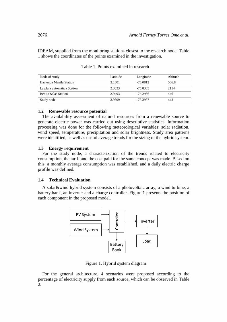
1.4 Technical Evaluation
A solar&wind hybrid system consists of a photovoltaic array, a wind turbine, a
battery bank, an inverter and a charge controller. Figure 1 presents the position of
each component in the proposed model.
Figure 1. Hybrid system diagram
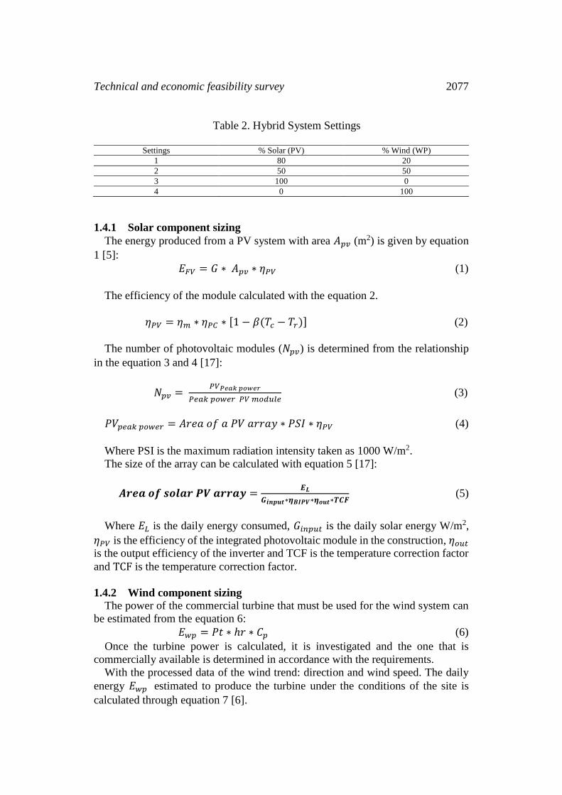
For the general architecture, 4 scenarios were proposed according to the
percentage of electricity supply from each source, which can be observed in Table
2.
Technical and economic feasibility survey 2077
Table 2. Hybrid System Settings
Settings % Solar (PV) % Wind (WP)
1 80 20
2 50 50
3 100 0
4 0 100
1.4.1 Solar component sizing
The energy produced from a PV system with area 𝐴𝑝𝑣 (m2) is given by equation
1 [5]:
𝐸𝐹𝑉 = 𝐺 ∗ 𝐴𝑝𝑣 ∗ 𝜂𝑃𝑉 (1)
The efficiency of the module calculated with the equation 2.
𝜂𝑃𝑉 = 𝜂𝑚 ∗ 𝜂𝑃𝐶 ∗ [1 − 𝛽(𝑇𝑐 − 𝑇𝑟)] (2)
The number of photovoltaic modules (𝑁𝑝𝑣) is determined from the relationship
in the equation 3 and 4 [17]:
𝑁𝑝𝑣 = 𝑃𝑉𝑃𝑒𝑎𝑘 𝑝𝑜𝑤𝑒𝑟
𝑃𝑒𝑎𝑘 𝑝𝑜𝑤𝑒𝑟 𝑃𝑉 𝑚𝑜𝑑𝑢𝑙𝑒 (3)
𝑃𝑉𝑝𝑒𝑎𝑘 𝑝𝑜𝑤𝑒𝑟 = 𝐴𝑟𝑒𝑎 𝑜𝑓 𝑎 𝑃𝑉 𝑎𝑟𝑟𝑎𝑦 ∗ 𝑃𝑆𝐼 ∗ 𝜂𝑃𝑉 (4)
Where PSI is the maximum radiation intensity taken as 1000 W/m2.
The size of the array can be calculated with equation 5 [17]:
𝑨𝒓𝒆𝒂 𝒐𝒇 𝒔𝒐𝒍𝒂𝒓 𝑷𝑽 𝒂𝒓𝒓𝒂𝒚 =𝑬𝑳
𝑮𝒊𝒏𝒑𝒖𝒕∗𝜼𝑩𝑰𝑷𝑽∗𝜼𝒐𝒖𝒕∗𝑻𝑪𝑭 (5)
Where 𝐸𝐿 is the daily energy consumed, 𝐺𝑖𝑛𝑝𝑢𝑡 is the daily solar energy W/m2,
𝜂𝑃𝑉 is the efficiency of the integrated photovoltaic module in the construction, 𝜂𝑜𝑢𝑡
is the output efficiency of the inverter and TCF is the temperature correction factor
and TCF is the temperature correction factor.
1.4.2 Wind component sizing
The power of the commercial turbine that must be used for the wind system can
be estimated from the equation 6:
𝐸𝑤𝑝 = 𝑃𝑡 ∗ ℎ𝑟 ∗ 𝐶𝑝 (6)
Once the turbine power is calculated, it is investigated and the one that is
commercially available is determined in accordance with the requirements.
With the processed data of the wind trend: direction and wind speed. The daily
energy 𝐸𝑤𝑝 estimated to produce the turbine under the conditions of the site is
calculated through equation 7 [6].
2078 Arnold Ferney Torres Ome et al.
𝐸𝑤𝑝 =1
2𝜌𝐴𝑉3 (7)
Where 𝜌 is the air density, A is the flow area and V is the average wind speed.
1.4.3 Inverter sizing
The selected inverter should be able to withstand the maximum expected energy
of DC loads. The output capacity of the inverter must be greater than the power of
the total DC loads. The conversion efficiency to the minimum load should be at
least 80% [17].
The nominal power of the inverter is calculated from the expression 8, where the
power factor is normally provided by the manufacturer.
𝑃𝑘𝑉𝐴 =𝑃ℎ𝑤𝑓𝑣
𝑃𝑜𝑤𝑒𝑟 𝑓𝑎𝑐𝑡𝑜𝑟 (8)
The input energy per day to the inverter 𝐸𝐼𝑁𝑉, where the efficiency 𝜂𝐼𝑁𝑉 is given
by the manufacturer as shown in equation 9:
𝐸𝐼𝑁𝑉 =𝐸ℎ𝑤𝑓𝑣
𝜂𝐼𝑁𝑉 (9)
1.4.4 Storage sizing
The storage capacity of the battery can be calculated according to equation 10:
[6]:
𝑆𝑡𝑜𝑟𝑎𝑔𝑒 𝑐𝑎𝑝𝑎𝑐𝑖𝑡𝑦 =𝑁𝐶∗𝐸𝐿
𝐷𝑂𝐷∗𝜂𝑜𝑢𝑡 (10)
The battery life is a function of the maximum depth of discharge, taken as 0.8.
The method for storage design is based on the energy supply concept during the
number of autonomous days; during these days the demand for energy is satisfied
only with the energy storage system.
If Nc is the largest number of autonomous days, then the minimum hourly
amperes of the battery are determined by equation 11:
𝐴ℎ𝑡𝑜𝑡𝐵 =𝑆𝑡𝑜𝑟𝑎𝑔𝑒 𝑐𝑎𝑝𝑎𝑐𝑖𝑡𝑦
𝐷𝐶 𝑛𝑜𝑚𝑖𝑛𝑎𝑙 𝑣𝑜𝑙𝑡𝑎𝑔𝑒 (11)
The energy storage capacity of the battery (𝐵𝐴𝐴ℎ) is determined by the daily
energy requirement (𝐸𝑖𝑛𝑣) and by the number of days of backup (𝑀𝐵𝑎𝑐𝑘𝑢𝑝) using
equation 12, [14]:
𝐵𝐴𝐴ℎ =𝐸𝑖𝑛𝑣 ∗ 𝑀𝐵𝑎𝑐𝑘𝑢𝑝
𝑉𝑖𝑛,𝐷𝐶 ∗ 𝐷𝑂𝐷 (12)
1.4.5 Design of the battery charge controller
The primary function of a charge controller in an independent power system is to
keep the battery in the highest possible state of charge, protecting it from
overloading the network and overloading.

Technical and economic feasibility survey 2079
The charge controller is generally dimensioned in such a way that it performs its
control function. A suitable charge controller must be able to withstand the set
current, as well as the total load current and it must be designed to match the voltage
of the photovoltaic solar module, wind turbine, as well as that of the battery bank.
The MPPT charge controller is specified according to the voltage handling
capacity. Nowadays, the charge controller usually comes with the inverter. There is
a recommended voltage range, within which must choose the DC voltage of the
power generating system.
1.5 Total Cost of Hybrid System
The first step in the economic evaluation was the determination of costs. These
were divided into components, installation and others.
The costs of the components were evaluated including photovoltaic and wind. A
synthesis of the cost in dollars was made according to the information availability.
The installation costs are related to construction, civil works, engineering and
contingencies; which were calculated from 30% of the cost of each panel and
turbine respectively [13].
For other components such as wiring, metal structure, grounding, protection
systems, small distribution towers and lifting services; they were estimated with
10% of the global cost [13].
During operation and maintenance, equation 13 was considered to calculate the
related costs during such period, taking as an initial point 1% for the photovoltaic
component and 3% for the turbines, a value equivalent to the maintenance of the
first year.
𝐶𝑎𝑚𝑎𝑖𝑛(𝑛) = 𝐶𝑎𝑚𝑎𝑖𝑛(1) ∗ (1 + 𝑓)𝑛 (13)
The dismantling was determined from the methodology of level costs of the
International Energy Agency (IEA), where they are estimated at 5% of the cost of
installing panels and turbines respectively [13].
Thus, the total cost is determined as the sum of each of the mentioned aspects as
can be seen in expression 14.
𝐶ℎ𝑤𝑓𝑣 = 𝐶𝑓𝑣 + 𝐶𝑤𝑝 + 𝐶𝑖𝑛𝑠𝑡 + 𝐶𝑂&𝑀 + 𝐶𝑑𝑒𝑠𝑚 (14)
1.6 Economic evaluation
1.6.1 Levelized cost of energy
The system costs analysis also plays an important role in the analysis of a hybrid
system. There are several ways to perform a cost analysis for the system. The
analysis of the levelized cost of energy (LCE) can be one of them, defined as the
relation of the cost of the total annual system 𝐶𝐴_𝑡𝑜𝑡𝑎𝑙 and the energy generated by
the system 𝐸𝑡𝑜𝑡𝑎𝑙, given by the expression 15, [9].
𝐿𝐶𝐸 = 𝐶𝐴_𝑡𝑜𝑡𝑎𝑙
𝐸𝑡𝑜𝑡𝑎𝑙 (15)
2080 Arnold Ferney Torres Ome et al.
Another important factor that they have studied in [10], is the Annual Life Cycle
Cost – ALCC, which includes the Life Cycle Cost – LCC, equation 16: [9].
𝐴𝐿𝐶𝐶 = 𝐶𝑅𝐹 ∗ 𝐿𝐶𝐶 (16)
Considering the influence of the increase in the cost of annual maintenance and
operating costs, the capital recovery factor CRF was used, as shown in equation 17
[9].
𝐶𝑅𝐹 = 𝑑(1+𝑑)𝑡
[(1+𝑑)𝑡−1] (17)
Where d is the discount rate that is the profitability that the financial entities offer
for capital investment (2.7% taken for this case) and t is the life time of the Project.
1.6.2 Net Present Value – NPV
The net present value as the total present value, which includes the initial cost of
the system, the repair and maintenance cost [11]. The NPV compares the present
value with the future value, so that inflation is considered (Inflation for the study of
3.17%).
The NPV can be defined with the equation 18 [11]:
NPV = [(1 + (P
A))
1
q− 1]
q
− 1 (18)
Where 𝑞 =𝑙𝑜𝑔[1+(
1
𝑁)]
log 2, P is the amount to pay, A is the initial cost and N is the
number of payments 𝑁 = 𝑛 ∗ 12.
1.6.3 Payback period
The Payback Period - PBP is calculated by means of the total investment cost
divided by the income of the first year by the energy saved, displaced or produced.
In the period analysis of investment recovery, the unit of measure is the number of
years to recover the investment from the total cost of the system. Projects with short
periods are perceived as having low risk [17].
1.6.4 Savings to investment ratio
The savings to investment ratio can be used to compare the savings with the costs
of the relative energy system with the alternative energy system. For positive net
savings, the SIR must be greater than one. High values of SIR present greater
savings relative to investment [17].
1.7 Reliability analysis
The reliability analysis consists in evaluating the system economically and
technically at the same time to determine if it is adequate and sufficient for the load
requirements that it will make subjected during its period of operation. For this

Technical and economic feasibility survey 2081
process, the LCE evaluation and Loss Power Supply Probability - LPSP are
sometimes used.
There are several methodologies for this purpose: probabilistic, analytical,
iterative, graphic, technical optimization and multi-objective, and in general using
computerized tools [5]–[9].
1.7.1 LPSP Analysis
Due to the variation of climatic conditions, sometimes the energy produced from
renewable sources cannot be estimated correctly, in these cases it is common to use
a reliability analysis for the designed hybrid system, which consists in evaluating
the Loss power supply probability. This parameter has been studied in [9], [10],
[18].
Some studies propose expression 18 for the calculation of LPSP [19], [20]:
𝐿𝑃𝑆𝑃 =∑ 𝐿𝑃𝑆(𝑡)𝑇
𝑡=1
∑ 𝐸𝐿(𝑡)𝑇𝑡=1
(19)
Where LPS (t) is determined with the expression 19.
𝐿𝑃𝑆(𝑡) = 𝐸𝐿(𝑡) − (𝐸𝐺𝐴(𝑡) + 𝐸𝐵(𝑡 − 1) − 𝐸𝐵𝑚𝑖𝑛) ∗ 𝜂𝑖𝑛𝑣 (20)
1.8 Optimization and sensitivity cases
With the information about the meteorological data, the electric charge required
and the technical-economic design of the system, it was proceeded to model the
hybrid system with all its components in the software Hybrid Optimization Model
of Electric Renewable - HOMER, which is commonly used for the modelling of
processes and energy systems, especially renewable energy systems.
Results
1.9 Electrical requirements
Figure 2 shows the trend of the kWh consumed by the residence object of study
in the period between 2012 and 2016.
Figure 2 Monthly electricity consumption
2082 Arnold Ferney Torres Ome et al.
It was possible to identify that the months with the highest consumption were
April (478 kWh) followed by the month of February (476 kWh), January (469 kWh)
and July (469 kWh). The months with the lowest consumption were June (430 kWh)
and December (428 kWh). The latter could be due to holidays and/or periods of
recess that the inhabitants of the residence have in common.
In general, the descriptive analysis showed that the electric power consumption
in kWh ranged from 375 kWh (minimum value) to 566 kWh (maximum value),
obtaining an average value of 458 kWh.
On the other hand, based on Figure 2 it can be inferred that the rates are not
constant. Since 2013, there has been an increase in rates, which becomes more
noticeable between 2015 and 2016. It is then that between 2013 and 2014 the rate
increased by 6%, between 2014 and 2015 a value of 4%, but between 2015 and
2016 it increased by 10% considering only the annual change, because if it is
evaluated between 2013 and 2016 an increase of 25% is presented.
The average monthly rate ranged between a minimum value of $ 0.135 USD/kWh
and a maximum value of $ 0.144 USD/ kWh. It also has that the average value in
the years studied is 0.139 USD/kWh per month. The costs paid presented an average
value of $ 63.69 USD, with a maximum of $ 84.37 USD in the month of July 2014.
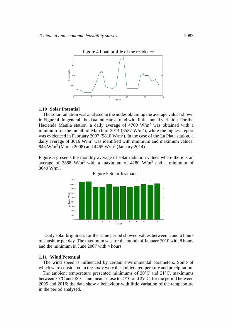
1.9.1 Load requirement estimations
Based on the history of the bills and a daily analysis made during a month to the
consumption that occurs in the house. It was determined that the average value of
the consumption on the day was 15.62 kWh-day considering the peak hours where
the highest consumption is generated (Figure 3), which is at 6 am, at noon between
12 and 2 pm, and at night at 6 pm.
Figure 3 Electricity rate History
Technical and economic feasibility survey 2083
Figure 4 Load profile of the residence
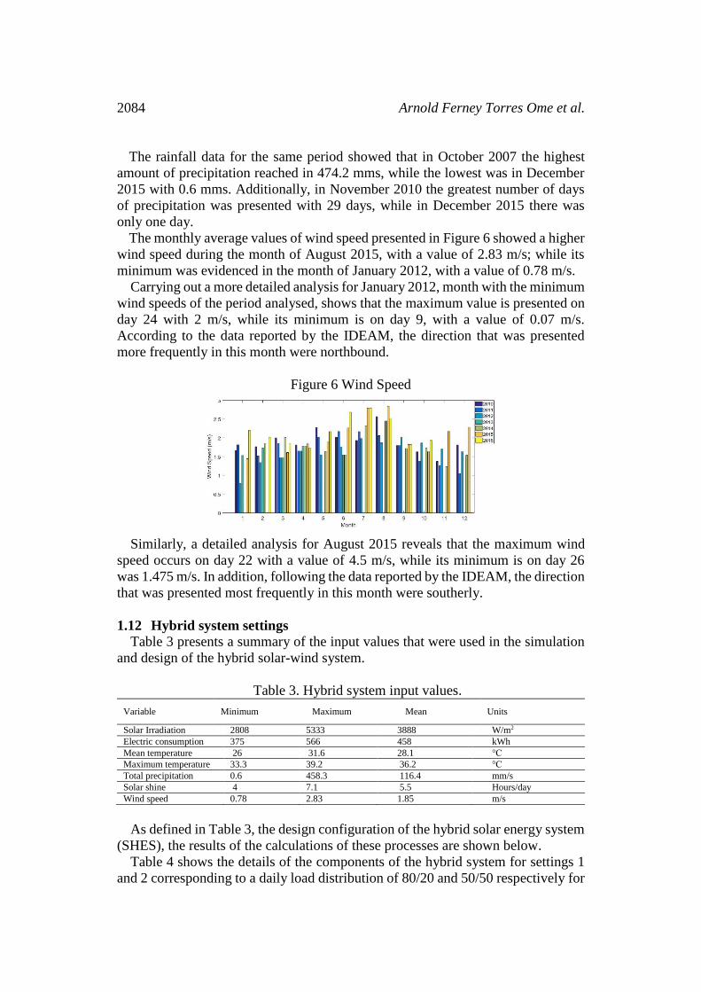
1.10 Solar Potential
The solar radiation was analysed in the nodes obtaining the average values shown
in Figure 4. In general, the data indicate a trend with little annual variation. For the
Hacienda Manila station, a daily average of 4760 W/m2 was obtained with a
minimum for the month of March of 2014 (3537 W/m2), while the highest report
was evidenced in February 2007 (5810 W/m2). In the case of the La Plata station, a
daily average of 3016 W/m2 was identified with minimum and maximum values:
843 W/m2 (March 2008) and 4465 W/m2 (January 2014).
Figure 5 presents the monthly average of solar radiation values where there is an
average of 3888 W/m2 with a maximum of 4280 W/m2 and a minimum of
3640 W/m2.
Figure 5 Solar Irradiance
Daily solar brightness for the same period showed values between 5 and 6 hours
of sunshine per day. The maximum was for the month of January 2010 with 8 hours
and the minimum in June 2007 with 4 hours.
1.11 Wind Potential
The wind speed is influenced by certain environmental parameters. Some of
which were considered in the study were the ambient temperature and precipitation.
The ambient temperature presented minimums of 20°C and 21°C, maximums
between 35°C and 38°C; and means close to 27°C and 29°C, for the period between
2005 and 2016; the data show a behaviour with little variation of the temperature
in the period analysed.
2084 Arnold Ferney Torres Ome et al.
The rainfall data for the same period showed that in October 2007 the highest
amount of precipitation reached in 474.2 mms, while the lowest was in December
2015 with 0.6 mms. Additionally, in November 2010 the greatest number of days
of precipitation was presented with 29 days, while in December 2015 there was
only one day.
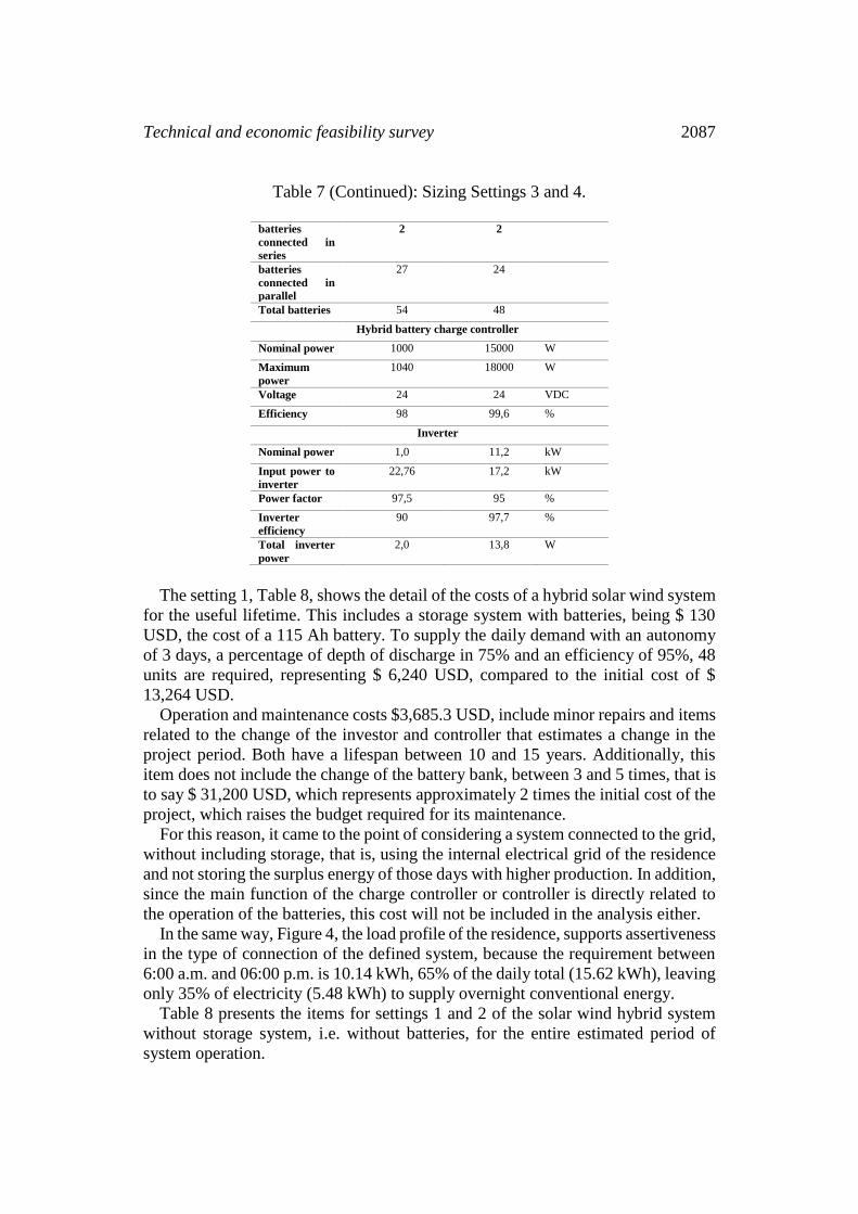
The monthly average values of wind speed presented in Figure 6 showed a higher
wind speed during the month of August 2015, with a value of 2.83 m/s; while its
minimum was evidenced in the month of January 2012, with a value of 0.78 m/s.
Carrying out a more detailed analysis for January 2012, month with the minimum
wind speeds of the period analysed, shows that the maximum value is presented on
day 24 with 2 m/s, while its minimum is on day 9, with a value of 0.07 m/s.
According to the data reported by the IDEAM, the direction that was presented
more frequently in this month were northbound.
Figure 6 Wind Speed
Similarly, a detailed analysis for August 2015 reveals that the maximum wind
speed occurs on day 22 with a value of 4.5 m/s, while its minimum is on day 26
was 1.475 m/s. In addition, following the data reported by the IDEAM, the direction
that was presented most frequently in this month were southerly.
1.12 Hybrid system settings
Table 3 presents a summary of the input values that were used in the simulation
and design of the hybrid solar-wind system.
Table 3. Hybrid system input values.
Variable Minimum Maximum Mean Units
Solar Irradiation 2808 5333 3888 W/m2
Electric consumption 375 566 458 kWh
Mean temperature 26 31.6 28.1 °C
Maximum temperature 33.3 39.2 36.2 °C
Total precipitation 0.6 458.3 116.4 mm/s
Solar shine 4 7.1 5.5 Hours/day
Wind speed 0.78 2.83 1.85 m/s
As defined in Table 3, the design configuration of the hybrid solar energy system
(SHES), the results of the calculations of these processes are shown below.
Table 4 shows the details of the components of the hybrid system for settings 1
and 2 corresponding to a daily load distribution of 80/20 and 50/50 respectively for

Technical and economic feasibility survey 2085
the PV/WP ratio. Setting 1 presents a system of 3.18 kW of installation power while
the second a system of 6.12 kW. Additionally, it could be found that the
performance for a photovoltaic system according to the module used and the Neiva
conditions was 19.69 kWh/kWp and for the wind resource 1.5 kWh/kWp
considering a turbine of 800W of power and average winds between 1.85 m/s and
2.39 m/s. It can be observed in the same way that the setting 1 that has the largest
number of photovoltaic modules has a higher energy generated.
Because of the solar conditions, the setting 3 that considers a system formed only
by photovoltaic modules, presents a greater generation of energy compared to the
setting 4 that considers a system only with turbines. Table 6 shows the details of
settings 3 and 4, where it is important to highlight 4 photovoltaic modules and 14
wind turbines, which shows a great difference in units that, will later influence a
representative difference in cost.
1.13 Hybrid system costs
The costs of the hybrid solar wind system were obtained from information
supplied by three national suppliers, one international supplier, considering the
availability of shipment to Colombia and the stock. A synthesis of the costs of each
component was made and at the end the lowest values were selected.
Table 4 Sizing Settings 1 and 2. Setting 1 2
Technology PV WP PV WP Units
Daily load 12,496 3,124 7,81 7,81 kWh-day
Nominal power 260 800 260 800 W
Quantity 3 3 2 7
Installed power 780 2400 520 5600 W
Performance 19,69 1,5 19,6 1,5 kWh/kWp
Output power 15,36 3,6 10,2 8,4 kWh-day
SHES total
power
3,18 6,12 kW
SHES output
power
18,96 18,64 kWh-day
Performance 5,96 3,05 kWh/kWp
Batteries
Voltage single
battery
12 12 VDC
Battery
capacity
115 115 Ah
Performance
battery bank
67455 69230 Wh
batteries
connected in
series
2 2
batteries
connected in
parallel
24 26
Total batteries 48 52

2086 Arnold Ferney Torres Ome et al.
Table 5 (Continued): Sizing Settings 1 and 2.
Hybrid battery charge controller
Nominal power 3200 10000 W
Maximum
power
6000 20000 W
Voltage 24 24 VDC
Efficiency 85 90 %
Inverter
Nominal power 3,21 6,18 kW
Input power to
inverter
19,45 19,12 kW
Power factor 99 95 %
Inverter
efficiency
97.5 95 %
Total inverter
power
3300 18000 W
It is important to mention that the inclusion of batteries or not to the hybrid
system, determines in large percentage an increase in the total cost of the system,
since it represents 47% of the initial cost and more than 100% of the operation and
maintenance costs due to the number of spare parts that must be carried out in the
25 years of the project. The batteries are designed to work in cycles of loading and
unloading, the greater the number of cycles the shorter the life time. Considering
that the battery bank operates every day under normal conditions, it would be
speaking of an approximate duration between 5 and 8 years, therefore, the number
of changes that must be made in the project period is between 3 and 5 times.
Table 6 Sizing Settings 3 and 4.
Settings 3 4
Technology PV WP PV WP Units
Daily load 15,62 15,62 kWh-day
Nominal power 260 800 W
Quantity 4 14
Installed power 1040 11200 W
Performance 19,69 1,5 kWh/kWp
Output power 20,48 16,8 kWh-day
SHES total
power
1,04 11,2
SHES output
power
20,48 16,8
Performance 19,69 1,5
Batteries
Voltage single
battery
12 12 VDC
Battery
capacity
115 115 Ah
Performance
battery bank
73076 67317 Wh
Technical and economic feasibility survey 2087
Table 7 (Continued): Sizing Settings 3 and 4.
batteries
connected in
series
2 2
batteries
connected in
parallel
27 24
Total batteries 54 48
Hybrid battery charge controller
Nominal power 1000 15000 W
Maximum
power
1040 18000 W
Voltage 24 24 VDC
Efficiency 98 99,6 %
Inverter
Nominal power 1,0 11,2 kW
Input power to
inverter
22,76 17,2 kW
Power factor 97,5 95 %
Inverter
efficiency
90 97,7 %
Total inverter
power
2,0 13,8 W
The setting 1, Table 8, shows the detail of the costs of a hybrid solar wind system
for the useful lifetime. This includes a storage system with batteries, being $ 130
USD, the cost of a 115 Ah battery. To supply the daily demand with an autonomy
of 3 days, a percentage of depth of discharge in 75% and an efficiency of 95%, 48
units are required, representing $ 6,240 USD, compared to the initial cost of $
13,264 USD.
Operation and maintenance costs $3,685.3 USD, include minor repairs and items
related to the change of the investor and controller that estimates a change in the
project period. Both have a lifespan between 10 and 15 years. Additionally, this
item does not include the change of the battery bank, between 3 and 5 times, that is
to say $ 31,200 USD, which represents approximately 2 times the initial cost of the
project, which raises the budget required for its maintenance.
For this reason, it came to the point of considering a system connected to the grid,
without including storage, that is, using the internal electrical grid of the residence
and not storing the surplus energy of those days with higher production. In addition,
since the main function of the charge controller or controller is directly related to
the operation of the batteries, this cost will not be included in the analysis either.
In the same way, Figure 4, the load profile of the residence, supports assertiveness
in the type of connection of the defined system, because the requirement between
6:00 a.m. and 06:00 p.m. is 10.14 kWh, 65% of the daily total (15.62 kWh), leaving
only 35% of electricity (5.48 kWh) to supply overnight conventional energy.
Table 8 presents the items for settings 1 and 2 of the solar wind hybrid system
without storage system, i.e. without batteries, for the entire estimated period of
system operation.
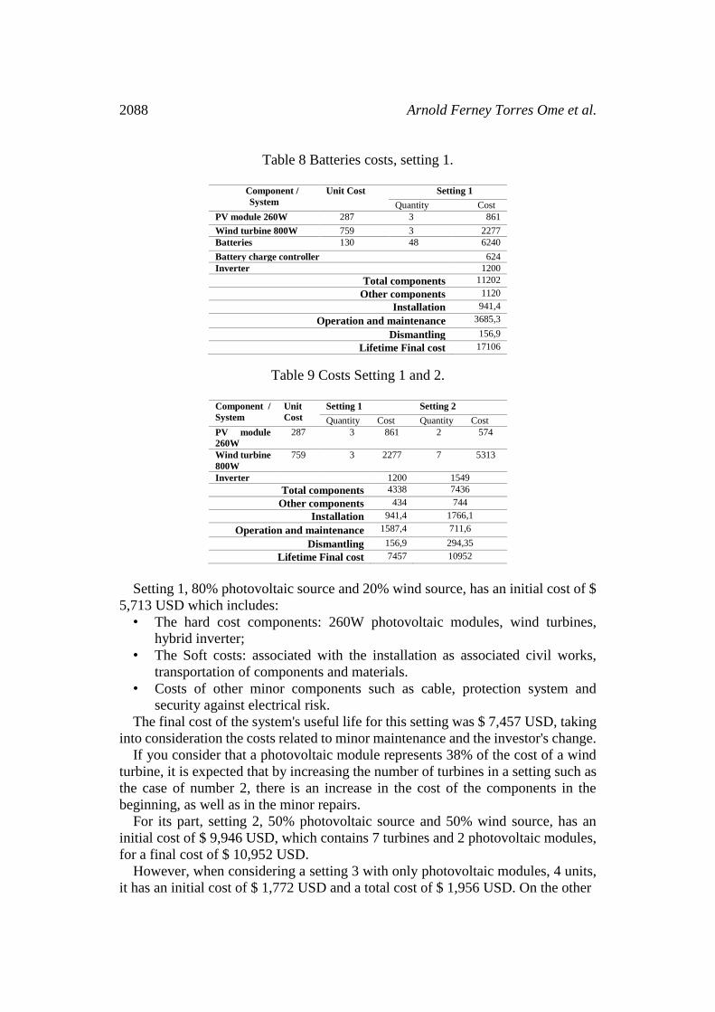
2088 Arnold Ferney Torres Ome et al.
Table 8 Batteries costs, setting 1.
Component /
System
Unit Cost Setting 1
Quantity Cost
PV module 260W 287 3 861
Wind turbine 800W 759 3 2277
Batteries 130 48 6240
Battery charge controller 624
Inverter 1200
Total components 11202
Other components 1120
Installation 941,4
Operation and maintenance 3685,3
Dismantling 156,9
Lifetime Final cost 17106
Table 9 Costs Setting 1 and 2.
Component /
System
Unit
Cost
Setting 1 Setting 2
Quantity Cost Quantity Cost
PV module
260W
287 3 861 2 574
Wind turbine
800W
759 3 2277 7 5313
Inverter 1200 1549
Total components 4338 7436
Other components 434 744
Installation 941,4 1766,1
Operation and maintenance 1587,4 711,6
Dismantling 156,9 294,35
Lifetime Final cost 7457 10952
Setting 1, 80% photovoltaic source and 20% wind source, has an initial cost of $
5,713 USD which includes:
• The hard cost components: 260W photovoltaic modules, wind turbines,
hybrid inverter;
• The Soft costs: associated with the installation as associated civil works,
transportation of components and materials.
• Costs of other minor components such as cable, protection system and
security against electrical risk.
The final cost of the system's useful life for this setting was $ 7,457 USD, taking
into consideration the costs related to minor maintenance and the investor's change.
If you consider that a photovoltaic module represents 38% of the cost of a wind
turbine, it is expected that by increasing the number of turbines in a setting such as
the case of number 2, there is an increase in the cost of the components in the
beginning, as well as in the minor repairs.
For its part, setting 2, 50% photovoltaic source and 50% wind source, has an
initial cost of $ 9,946 USD, which contains 7 turbines and 2 photovoltaic modules,
for a final cost of $ 10,952 USD.
However, when considering a setting 3 with only photovoltaic modules, 4 units,
it has an initial cost of $ 1,772 USD and a total cost of $ 1,956 USD. On the other
Technical and economic feasibility survey 2089
hand, a system based 100% on wind power has an initial cost of $ 19,069 USD
which includes the use of 14 turbines of 800W to supply the energy demand,
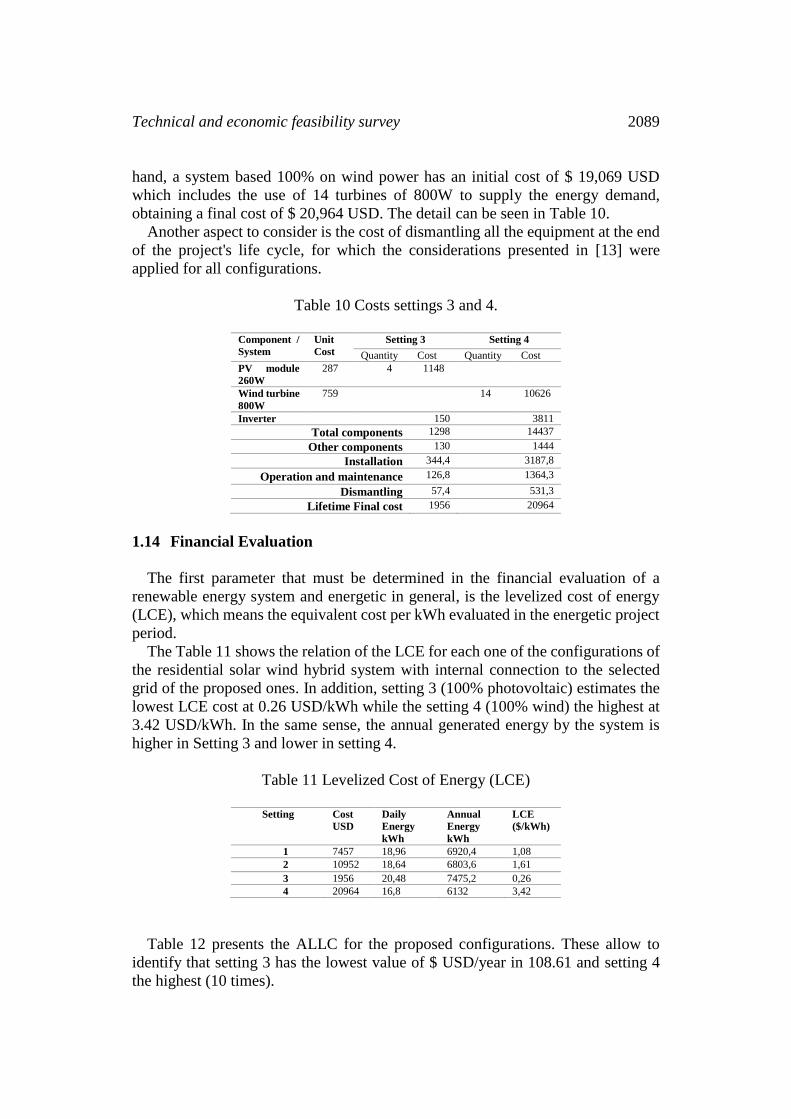
obtaining a final cost of $ 20,964 USD. The detail can be seen in Table 10.
Another aspect to consider is the cost of dismantling all the equipment at the end
of the project's life cycle, for which the considerations presented in [13] were
applied for all configurations.
Table 10 Costs settings 3 and 4.
Component /
System
Unit
Cost
Setting 3 Setting 4
Quantity Cost Quantity Cost
PV module
260W
287 4 1148
Wind turbine
800W
759
14 10626
Inverter 150 3811
Total components 1298 14437
Other components 130 1444
Installation 344,4 3187,8
Operation and maintenance 126,8 1364,3
Dismantling 57,4 531,3
Lifetime Final cost 1956 20964
1.14 Financial Evaluation
The first parameter that must be determined in the financial evaluation of a
renewable energy system and energetic in general, is the levelized cost of energy
(LCE), which means the equivalent cost per kWh evaluated in the energetic project
period.
The Table 11 shows the relation of the LCE for each one of the configurations of
the residential solar wind hybrid system with internal connection to the selected
grid of the proposed ones. In addition, setting 3 (100% photovoltaic) estimates the
lowest LCE cost at 0.26 USD/kWh while the setting 4 (100% wind) the highest at
3.42 USD/kWh. In the same sense, the annual generated energy by the system is
higher in Setting 3 and lower in setting 4.
Table 11 Levelized Cost of Energy (LCE)
Setting Cost
USD
Daily
Energy
kWh
Annual
Energy
kWh
LCE
($/kWh)
1 7457 18,96 6920,4 1,08
2 10952 18,64 6803,6 1,61
3 1956 20,48 7475,2 0,26
4 20964 16,8 6132 3,42
Table 12 presents the ALLC for the proposed configurations. These allow to
identify that setting 3 has the lowest value of $ USD/year in 108.61 and setting 4
the highest (10 times).

2090 Arnold Ferney Torres Ome et al.
Table 12 Annual Life Cycle Cost
Setting Cost USD Annual
Energy
kWh
ALCC
($/year)
1 7457 6920,4 414,05
2 10952 6803,6 608,11
3 1956 7475,2 108,61
4 20964 6132 1164,03
The next step with LCE or ALCC values is to evaluate the net present value NPV,
which corresponds to the total cost of the project in the future. Table 13 shows the
values for the proposed options and highlights the setting 3 as the one with the
lowest cost in the future.
Table 13 Net Present Value
Setting Total
Cost
Initial
Cost
Net Present Value
(NPV)
1 7457 5713 9733,4
2 10952 9946 12059,8
3 1956 1772 2159,1
4 20964 19069 23047,3
Another important factor to consider in this section is the economic benefit that
the State grants to those who invest in projects that involve the use of renewable
energy technologies. According to the law 1715 of May 3, 2014, those who invest
in unconventional sources of energy will be able to access to a series of tax
incentives, the most outstanding is the exception of the payment of VAT and the
reduction of the declaration of income up to 50 %. Being the latest one interest and
predominant to those taxpayers who must pay their taxes by income statement, due
to, according to the tax reform of the law 1819 from December 29, 2016 that started
into rigor from January 1, 2017, all-natural people or legal entities that own real
property by proper noun that exceed $ 47,572 USD must pay taxes for this concept.
In view of the foregoing, considering that the objective residence of the project
design exceeds the stipulated value, that is, that the owner must pay taxes to the
State for exceeding these values, it is pertinent to propose a scenario where the
second benefit is included in the economic evaluation of the project, since it
presents indirectly a saving to the owner of the real property.
Table 14 shows the detail of the calculations that consider the tax benefit of the
discount of 50% of the initial investment, can be detailed in the column headed
"Desc 1715 Law" as well as the new final total cost of each of the proposed
configurations. On the other hand, Table 15 shows the new calculation of the LCE
with the new defined costs. It shows that configuration 3 continues taking the lowest
value followed by setting 1.
Technical and economic feasibility survey 2091
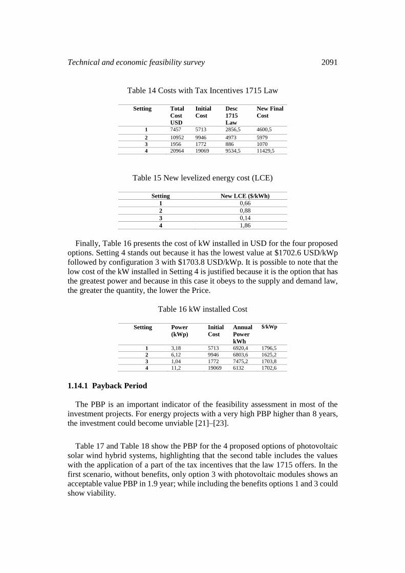
Table 14 Costs with Tax Incentives 1715 Law
Setting Total
Cost
USD
Initial
Cost
Desc
1715
Law
New Final
Cost
1 7457 5713 2856,5 4600,5
2 10952 9946 4973 5979
3 1956 1772 886 1070
4 20964 19069 9534,5 11429,5
Table 15 New levelized energy cost (LCE)
Setting New LCE ($/kWh)
1 0,66
2 0,88
3 0,14
4 1,86
Finally, Table 16 presents the cost of kW installed in USD for the four proposed
options. Setting 4 stands out because it has the lowest value at $1702.6 USD/kWp
followed by configuration 3 with $1703.8 USD/kWp. It is possible to note that the
low cost of the kW installed in Setting 4 is justified because it is the option that has
the greatest power and because in this case it obeys to the supply and demand law,
the greater the quantity, the lower the Price.
Table 16 kW installed Cost
Setting Power
(kWp)
Initial
Cost
Annual
Power
kWh
$/kWp
1 3,18 5713 6920,4 1796,5
2 6,12 9946 6803,6 1625,2
3 1,04 1772 7475,2 1703,8
4 11,2 19069 6132 1702,6
1.14.1 Payback Period
The PBP is an important indicator of the feasibility assessment in most of the
investment projects. For energy projects with a very high PBP higher than 8 years,
the investment could become unviable [21]–[23].
Table 17 and Table 18 show the PBP for the 4 proposed options of photovoltaic
solar wind hybrid systems, highlighting that the second table includes the values
with the application of a part of the tax incentives that the law 1715 offers. In the
first scenario, without benefits, only option 3 with photovoltaic modules shows an
acceptable value PBP in 1.9 year; while including the benefits options 1 and 3 could
show viability.

2092 Arnold Ferney Torres Ome et al.
Table 17 Payback period
Setting Total
Cost (P)
Annual
Power
kWh
Saving per
Generated
energy in 1
year (USD)
PBP
1 7457 6920,4 967 7,7
2 10952 6803,6 950 11,5
3 1956 7475,2 1044 1,9
4 20964 6132 856 24,5
Table 18 PBP with Law 1715 Benefits
Setting Total
Cost (P)
Annual
Power
kWh
Saving per
Generated
energy in 1
year (USD)
PBP
1 4600 6920 967 4,8
2 5979 6803 950 6,3
3 1070 7475 1044 1,0
4 11429 6132 856 13,3
The saving-investment ratio, Table 19 shows that in common all the values are
higher than 1, which is the expected positive behaviour, due to one of the aims of a
renewable energy system is the search for economic savings and this value
represents this trend. Option 3 stands out for having a high SIR.
Table 19 Savings and investment ratio (SIR)
Setting Total
Cost
Saving per
generated energy in
25 years
SIR
1 7457 24.164 3,2
2 10952 23.756 2,2
3 1956 26.101 13,3
4 20964 21.411 1,0
1.15 Reliability analysis
1.15.1 LPSP analysis
The calculations for the 4 proposed configurations show that the systems, despite
the variations of the wind and solar resource during the year, fulfil with the energy
supply, since it presents values between 0 and 0.25, highlighting that the setting 3
presented the lower value.

Technical and economic feasibility survey 2093
1.16 Optimization and sensitivity cases
Thanks to the versatilities that HOMER presents, variations of energy sources in
the different sensitivity scenarios, only 3 cases were considered. The first where the
settings 1 and 2 are evaluated, the second for setting 4 and the third for setting 3.
1.16.1 Case 1: Settings 1 and 2.
In this scenario, the hybrid combinations between the wind and solar resource are
considered, in addition the contribution of the grid and a diesel generator are
considered. Some of the initial economic conditions are a real discount rate of
2.74%, inflation rate of 3.17%, project life 25 years and an initial capital cost of $
4338 USD.
The simulation was carried out by finding 86,322 solutions of which 86,313 were
omitted due to financial infeasibility or minimum renewable fraction. The basic
simulation scheme in Figure 7 shows the components included in the calculations
made.
Figure 7 HOMER Diagram for Setting 1
Table 20 HOMER Simulation. Setting 1
Wind Scaled
Aver (m/s)
COE (USD) NPC
(USD)
Ren Fracc
(%)
CO2
(kg/yr)
1,85 $0,190 $12.588 50 1.170
3,0 $0,190 $12.588 50 1.170
8,0 $0,179 $11.878 62,3 881
1,85 $0,190 $12.588 50 1.170
3,0 $0,190 $12.588 50 1.170
8,0 $0,179 $11.878 62,3 881
1,85 $0,190 $12.588 50 1.170
3,0 $0,190 $12.588 50 1.170
8,0 $0,179 $11.878 62,3 881
Table 20 shows the 9 solutions selected for having the lowest cost of energy COE
and the largest fraction of renewable sources, presents combinations that include
2094 Arnold Ferney Torres Ome et al.
random groups among turbines, photovoltaic modules, batteries, grid connection
and diesel generator. Although the latest was excluded from the selection. There
are 3 combinations with a lower COE of $ 0.179 USD / kWh, a NPC of $ 11,878
USD and a renewable fraction of 62.3%.
It can be observed that the CO2 produced by the same solution in 881 Kg/yr as
well as inverse trends between the COE, NPC and the renewable fraction, because
as the fraction decreases, the other two variables increase. On the other hand, if it
is analyse the wind speed average scale considered for each case, we can deduce
that it is proportional to the renewable fraction and for the solution presented and it
has a value of 8 m/s, a value that according to the analysis of the Wind energy
resource does not occur in Neiva since the average is 1.85 m/s and in the months
with the highest speed it is 2.85 m/s. Which makes the solution 1 is the closest to
the proposed configuration where the COE is at $ 0.190 USD/kWh, NPC at $
12.588 USD and a renewable fraction of 50%.
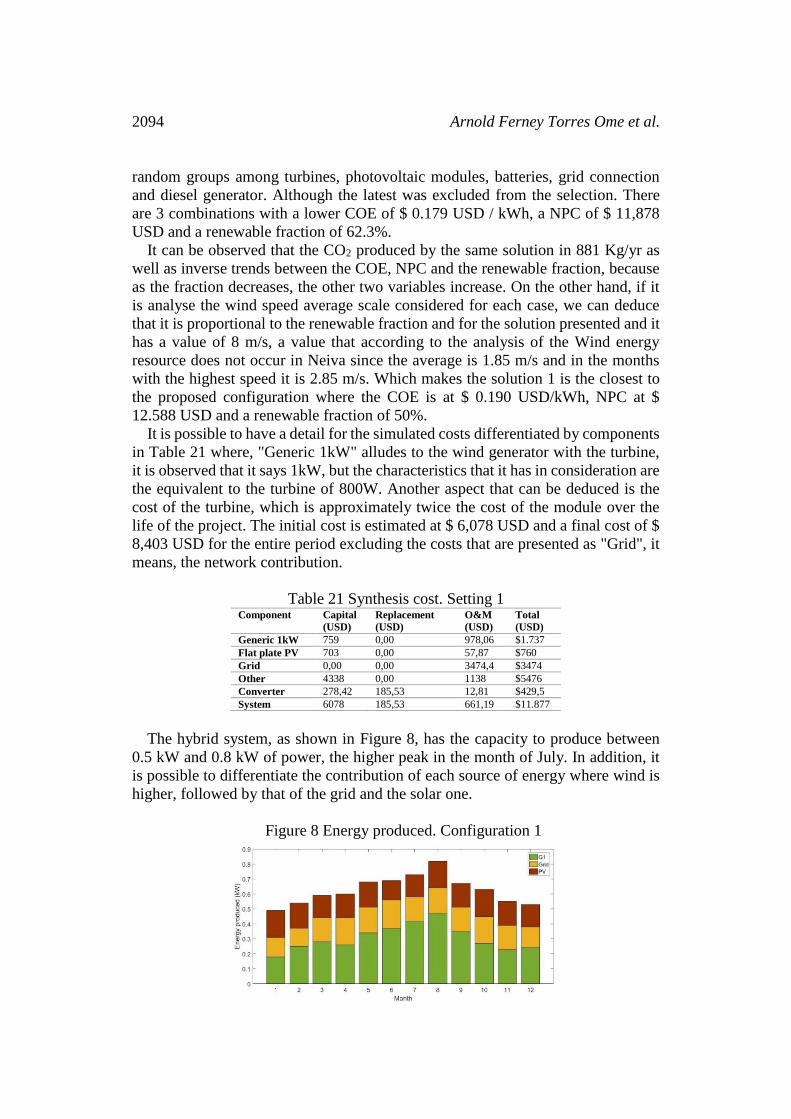
It is possible to have a detail for the simulated costs differentiated by components
in Table 21 where, "Generic 1kW" alludes to the wind generator with the turbine,
it is observed that it says 1kW, but the characteristics that it has in consideration are
the equivalent to the turbine of 800W. Another aspect that can be deduced is the
cost of the turbine, which is approximately twice the cost of the module over the
life of the project. The initial cost is estimated at $ 6,078 USD and a final cost of $
8,403 USD for the entire period excluding the costs that are presented as "Grid", it
means, the network contribution.
Table 21 Synthesis cost. Setting 1 Component Capital
(USD)
Replacement
(USD)
O&M
(USD)
Total
(USD)
Generic 1kW 759 0,00 978,06 $1.737
Flat plate PV 703 0,00 57,87 $760
Grid 0,00 0,00 3474,4 $3474
Other 4338 0,00 1138 $5476
Converter 278,42 185,53 12,81 $429,5
System 6078 185,53 661,19 $11.877
The hybrid system, as shown in Figure 8, has the capacity to produce between
0.5 kW and 0.8 kW of power, the higher peak in the month of July. In addition, it
is possible to differentiate the contribution of each source of energy where wind is
higher, followed by that of the grid and the solar one.
Figure 8 Energy produced. Configuration 1
Technical and economic feasibility survey 2095
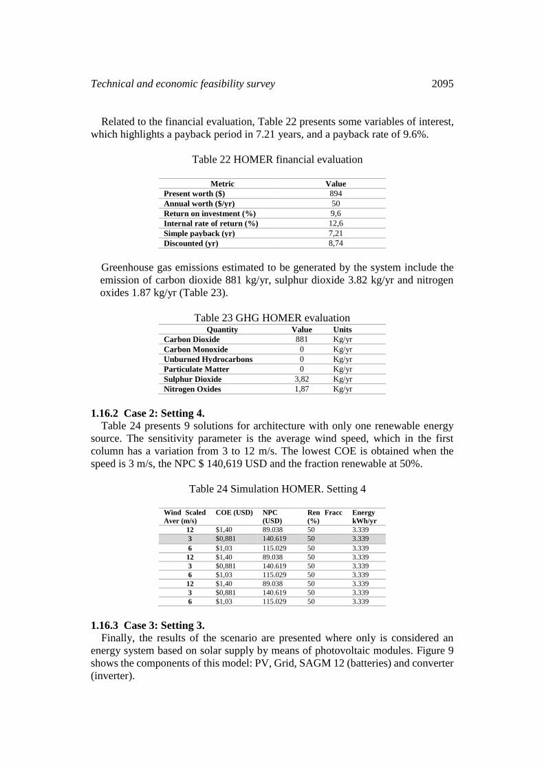
Related to the financial evaluation, Table 22 presents some variables of interest,
which highlights a payback period in 7.21 years, and a payback rate of 9.6%.
Table 22 HOMER financial evaluation
Metric Value
Present worth ($) 894
Annual worth ($/yr) 50
Return on investment (%) 9,6
Internal rate of return (%) 12,6
Simple payback (yr) 7,21
Discounted (yr) 8,74
Greenhouse gas emissions estimated to be generated by the system include the
emission of carbon dioxide 881 kg/yr, sulphur dioxide 3.82 kg/yr and nitrogen
oxides 1.87 kg/yr (Table 23).
Table 23 GHG HOMER evaluation Quantity Value Units
Carbon Dioxide 881 Kg/yr
Carbon Monoxide 0 Kg/yr
Unburned Hydrocarbons 0 Kg/yr
Particulate Matter 0 Kg/yr
Sulphur Dioxide 3,82 Kg/yr
Nitrogen Oxides 1,87 Kg/yr
1.16.2 Case 2: Setting 4.
Table 24 presents 9 solutions for architecture with only one renewable energy
source. The sensitivity parameter is the average wind speed, which in the first
column has a variation from 3 to 12 m/s. The lowest COE is obtained when the
speed is 3 m/s, the NPC $ 140,619 USD and the fraction renewable at 50%.
Table 24 Simulation HOMER. Setting 4
Wind Scaled
Aver (m/s)
COE (USD) NPC
(USD)
Ren Fracc
(%)
Energy
kWh/yr
12 $1,40 89.038 50 3.339
3 $0,881 140.619 50 3.339
6 $1,03 115.029 50 3.339
12 $1,40 89.038 50 3.339
3 $0,881 140.619 50 3.339
6 $1,03 115.029 50 3.339
12 $1,40 89.038 50 3.339
3 $0,881 140.619 50 3.339
6 $1,03 115.029 50 3.339
1.16.3 Case 3: Setting 3.
Finally, the results of the scenario are presented where only is considered an
energy system based on solar supply by means of photovoltaic modules. Figure 9
shows the components of this model: PV, Grid, SAGM 12 (batteries) and converter
(inverter).

2096 Arnold Ferney Torres Ome et al.
Figure 9 HOMER Diagram for Setting 3
4668 simulations were made of which only 9 presented one greater than 50%
renewable fraction. The parameter for cases of sensitivity was the nominal discount
rate, because while he was one of the initial values entered, the software used it to
obtain the solutions presented in Table 25. These are arranged in descending order,
where the last COE value of $0,0515 USD/kWh represents the best solution for
being the lowest cost of energy. In addition to this, has minor NPC in $8.537 USD
and a renewable fraction of 65.2%, the highest. The energy produced per year is
6.207 kWh to 3,309 kWh purchased the electric company to supply the
consumption during the hours of the night for a year. Two cases of optimization in
Table 26, presented correspondence with this trend, one without considering the
incorporation of batteries.
Table 25 Simulation HOMER. Setting 3
Nominal
Discount (%)
COE
(USD)
NPC
(USD)
Ren Fracc
(%)
Energy
kWh/yr
12 0,135 7.874 50 3.716
12 0,135 7.874 50 3.716
12 0,135 7.874 50 3.716
6 0,0738 8.421 62 5.537
6 0,0738 8.421 62 5.537
6 0,0738 8.421 62 5.537
3 0,0515 8.537 65,2 6.207
3 0,0515 8.537 65,2 6.207
3 0,0515 8.537 65,2 6.207
Table 26 Optimization HOMER. Setting 3
Nominal
Discount (%)
COE
(USD)
NPC
(USD)
Ren Fracc
(%)
Energy
kWh/yr)
3 0,0515 8.537 65,2 6.207
3 0,0530 8.781 65,2 6.209
The electricity produced per year is listed by source in Figure 10, where the
greatest contribution is from photovoltaic source 0.8 kW followed the night the
network supply approximate 0.4 kW.
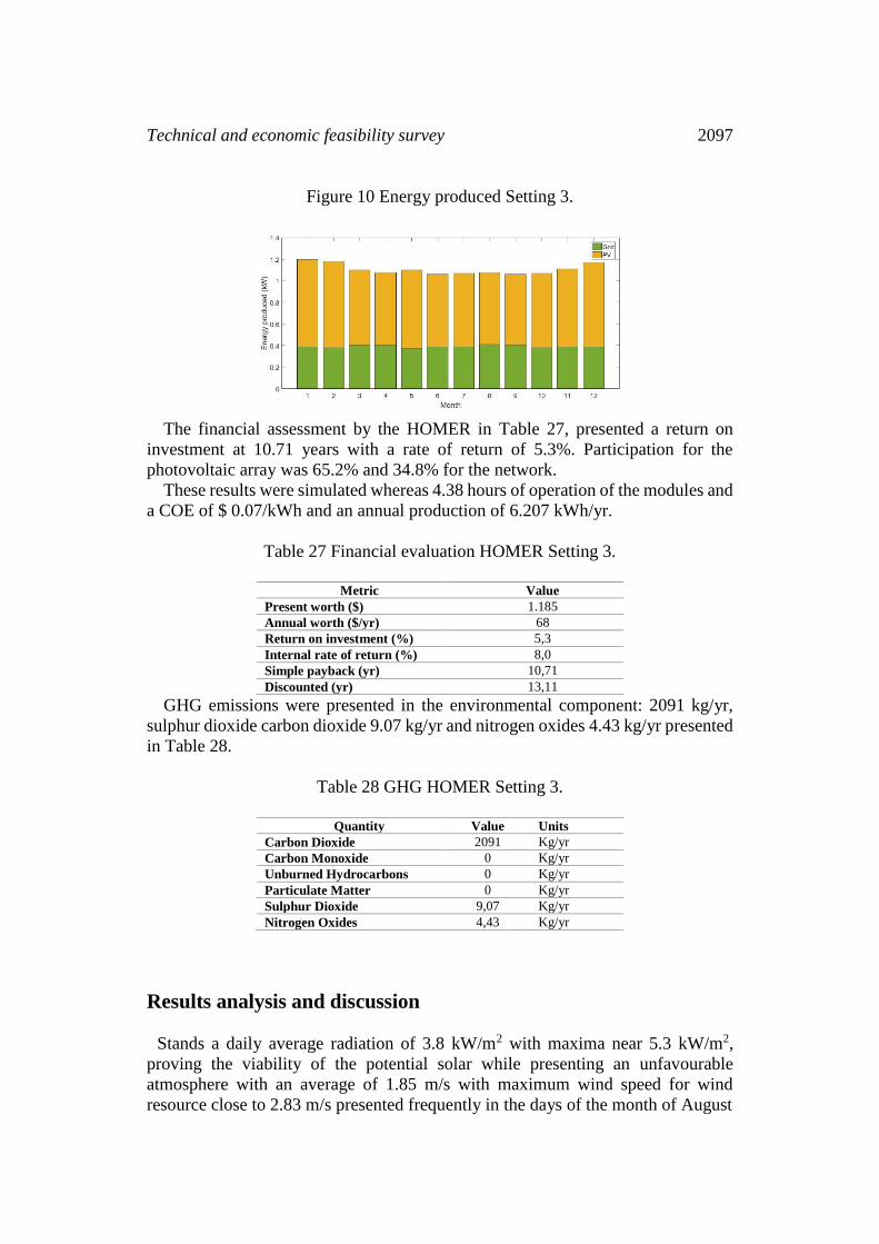
Technical and economic feasibility survey 2097
Figure 10 Energy produced Setting 3.
The financial assessment by the HOMER in Table 27, presented a return on
investment at 10.71 years with a rate of return of 5.3%. Participation for the
photovoltaic array was 65.2% and 34.8% for the network.
These results were simulated whereas 4.38 hours of operation of the modules and
a COE of $ 0.07/kWh and an annual production of 6.207 kWh/yr.
Table 27 Financial evaluation HOMER Setting 3.
Metric Value
Present worth ($) 1.185
Annual worth ($/yr) 68
Return on investment (%) 5,3
Internal rate of return (%) 8,0
Simple payback (yr) 10,71
Discounted (yr) 13,11
GHG emissions were presented in the environmental component: 2091 kg/yr,
sulphur dioxide carbon dioxide 9.07 kg/yr and nitrogen oxides 4.43 kg/yr presented
in Table 28.
Table 28 GHG HOMER Setting 3.
Quantity Value Units
Carbon Dioxide 2091 Kg/yr
Carbon Monoxide 0 Kg/yr
Unburned Hydrocarbons 0 Kg/yr
Particulate Matter 0 Kg/yr
Sulphur Dioxide 9,07 Kg/yr
Nitrogen Oxides 4,43 Kg/yr
Results analysis and discussion
Stands a daily average radiation of 3.8 kW/m2 with maxima near 5.3 kW/m2,
proving the viability of the potential solar while presenting an unfavourable
atmosphere with an average of 1.85 m/s with maximum wind speed for wind
resource close to 2.83 m/s presented frequently in the days of the month of August
2098 Arnold Ferney Torres Ome et al.
of the period studied. It is considered negative because the minimum speed required
to have any conventional turbine start to turn is at 3 m/s, which makes that he arises
a first statement about the technical infeasibility of a stand-alone wind power
system.
There are some turbines designed by ICEWIND for extreme conditions where
they consider minimum wind speed of 2 m/s. That case was not considered in the
evaluation because of unavailable any kind of technical information to perform the
exercise.
The power consumption of the node's study showed values between 375 and 566
with an average of 458 kWh kWh. At this point the profile load and a daily energy
requirement identified consumption of 15.62 kWh-day for a monthly total of 468
kWh.
Knowing the panorama of renewable energy sources: Sun and wind; as well as
the hypothesis of the wind resource was determined important to define 4
configurations of hybrid systems with the addition of an option for 100% PV and
the other to 100% wind energy.
Up now it had been considered standalone settings, i.e. isolated from
conventional electrical network, but due to the high amount of batteries requiring
every architectural design, between 48 and 54 units without considering the
replacement. According the costs related to the life cycle of batteries which means
a minimal change of 3 times the amount mentioned. It was decided to opt for a
system connected to grid providing a 65% of energy supply for electrical demand
during the hours of the day.
For configuration 1, System hybrid without replacement batteries had a cost of
$17.106 USD compared with $7.457 USD for Setup with connection to the grid, a
savings of 44% with respect to the first cost. For other configurations, the cost can
be seen in Table 29.
Moreover, technical feasibility is presented for settings 3 and 1 as they are those
that have lower costs and greater annual energy produced, if not evidenced when
the fraction of wind resource, WP is increased.
Table 29 Settings and costs.
Settings Fraction
(PV /WP)
Cost
USD
Daily Energy
kWh
Annual
Energy kWh
1 0,8 / 0,2 7457 18,96 6920,4
2 0,5 / 0,5 10952 18,64 6803,6
3 1,0 / 0 1956 20,48 7475,2
4 0 / 1,0 20964 16,8 6132
The financial evaluation, a sensitive but crucial topic at the time of an investment
of large sums of money was done by independent and correlated analysis of the
following economic parameters: the Levelized Cost of Energy LCE/COE, the
Technical and economic feasibility survey 2099
Annual Life Cycle Cost - ALCC, the net present value NPV, the payback period -
PBP, saving and investment – SIR and installed kW, within the most representative
patterns.
The setting 3 presented the best solution with a favourable for implementing
economic scenario, as it had the lowest LCE in 0.26 $USD/kWh, an allocation in
108,61 $USD/year and a future cost of $2.159,1 USD. The option with 100% wind
showed the reverse behaviour with high values. The lower cost of installed kW was
setting 4 as this presented the greatest power installed in 11.2 kW (wind turbines).
Having into account the tax incentives of Law 1715 as a reduction of income
taxes for the owner of the system and the residence. They presented a reduction of
50% of the initial cost and an additional 5% on the total cost of the project. The new
estimated cost of energy was 0.14 $USD/kWh for PV setting and 1.86 $USD/kWh
for wind power.
Additionally, the lower PBP was 1.9 years for the photovoltaic array and a pretty
good SIR in 13.3 which makes this configuration considered most appropriate for
the study area.
Conclusions
Weather conditions in the city of Neiva have favourable for harnessing energy
from solar resource as alternates to the hydroelectric plant. In contrast, the wind
resource is not suitable for use since there is wind speeds high and consistent to
consider their use and inclusion in the energy matrix of the Neiva area.
Architecture hybrid optima found, although it does not correspond to source
100% renewable, includes photovoltaic&solar resource and connection to grid to
supply the energy consumption with a distribution 65% and 35% respectively.
A System consideration of storage batteries in any configuration of hybrid
systems showed a non-viability of the residential projects due to the number of
spare parts because of the short time of life.
The inclusion of tax benefits reflects a relative advantage of a solar system
against the hydroelectric power as that present in 0,0515 $USD/kWh energy cost
values below the average cost of the energetic company in 0,139 $USD/kWh,
excluding the rate of annual increase that presented between 6% and 7%.
Due to the higher electrical consumption occurs between 6 am and 6 pm, allowed
that the load profile was favourable for the technical and economic calculations.
The results of optimization software HOMER proved to be very relevant to the
exercise because they provided solid tools for financial and environmental
assessment of the proposed settings.
2100 Arnold Ferney Torres Ome et al.
Future scope
The evaluation system of hybrid wind-solar performed identifies its infeasibility
in Neiva due to low wind speed presenting, but the behaviour of the wind resource
in the Department of Huila does not address what might be considered as a subject
of study for further research.
The load profile analysed in the study was that corresponding to the residential
area. Further studies could evaluate systems for the industrial zone of the city of
Neiva considering that most of the buildings in this area are its high-power
consumption during the hours of sunshine.
For the economic and financial evaluation were presented in a superficial manner
one of the benefits of the 1715 law for the promotion of renewable energy projects
but does not consider the impact of including all the benefits provided by the State
standard. An analysis of economic feasibility including all the deductions that can
be applied, could be considered as a target for a later work.
The energy matrix of the Department can be expanded by incorporating the
participation of non-conventional sources of energy. The region has other resources
such as groundwater, regions with agricultural and forest biomass, biogas,
geothermal reservoirs, municipal solid waste and some natural water currents. They
could both be considered to evaluate its potential in the region as to the
determination of the best configuration for an independent energy system or hybrid
to provide energy consumption of some population.
Acknowledgements. The authors are grateful to National Renewable Energy
Laboratory's - NREL in the United States for providing free license software
HOMER for the evaluation of the system and the Institute of hydrology,
meteorology and Environmental Studies - IDEAM by providing information of
meteorological variables, since thanks to the contributions made possible the
development of this work.
References
[1] Gobernación del Huila, CAM, E3, USAID, and FCMC, Plan cambio
climático Huila 2050: Preparándose para el cambio climático, 2014, 151.
[2] Gobernación del Huila and Cámara de Comercio de Neiva, Agenda Interna-
Plan Regional de Competitividad del Huila, 2015, 305.
[3] Congreso de Colombia, “Ley N° 1715 del 13 de mayo de 2014,” Upme, no.
May, 2014, 26.
Technical and economic feasibility survey 2101
[4] Instituto de hidrología meteorologia y estudios ambientales (IDEAM),
catálogo nacional de estaciones del IDEAM, 2017.
[5] S. Sinha and S. S. Chandel, Review of recent trends in optimization
techniques for solar photovoltaic-wind based hybrid energy systems, Renew.
Sustain. Energy Rev., 50 (2015), 755–769.
https://doi.org/10.1016/j.rser.2015.05.040
[6] V. Khare, S. Nema and P. Baredar, Solar-wind hybrid renewable energy
system: A review, Renew. Sustain. Energy Rev., 58 (2016), 23–33.
https://doi.org/10.1016/j.rser.2015.12.223
[7] T. Ma, H. Yang and L. Lu, A feasibility study of a stand-alone hybrid solar-
wind-battery system for a remote island, Appl. Energy, 121 (2014), 149–158.
https://doi.org/10.1016/j.apenergy.2014.01.090
[8] Y. Devrim and L. Bilir, Performance investigation of a wind turbine–solar
photovoltaic panels–fuel cell hybrid system installed at İncek region –
Ankara, Turkey, Energy Convers. Manag., 126 (2016), 759–766.
https://doi.org/10.1016/j.enconman.2016.08.062
[9] A. Mahesh and K. S. Sandhu, Hybrid wind/photovoltaic energy system
developments: Critical review and findings, Renew. Sustain. Energy Rev., 52
(2015), 1135–1147. https://doi.org/10.1016/j.rser.2015.08.008
[10] S. Diaf, M. Belhamel, M. Haddadi and A. Louche, Technical and economic
assessment of hybrid photovoltaic/wind system with battery storage in
Corsica island, Energy Policy, 36 (2008), no. 2, 743–754.
https://doi.org/10.1016/j.enpol.2007.10.028
[11] M. Esen and T. Yuksel, Experimental evaluation of using various renewable
energy sources for heating a greenhouse, Energy Build., 65 (2013), 340–351.
https://doi.org/10.1016/j.enbuild.2013.06.018
[12] A. Al-Sharafi, A. Z. Sahin, T. Ayar and B. S. Yilbas, Techno-economic
analysis and optimization of solar and wind energy systems for power
generation and hydrogen production in Saudi Arabia, Renew. Sustain. Energy
Rev., 69 (2017), 33–49. https://doi.org/10.1016/j.rser.2016.11.157
[13] A. Castillo, F. Villada and J. Valencia, Diseño multiobjetivo de un sistema

2102 Arnold Ferney Torres Ome et al.
híbrido eólico-solar con baterías para zonas no interconectadas, Revista
Tecnura, 18 (2014), no. 39, 77–93.
https://doi.org/10.14483/udistrital.jour.tecnura.2014.1.a06
[14] Y. Muñoz, J. Guerrero and A. Ospino, Evaluation of a hybrid system of
renewable electricity generation for a remote area of Colombia using homer
software, Tecciencia, 9 (2014), no. 17, 57–67.
https://doi.org/10.18180/tecciencia.2014.17.6
[15] L. M. Carrillo Medrano, Generación de energía con un sistema híbrido
renovable para abastecimiento básico en vereda sin energización de Yopal -
Casanare, 2015.
[16] I. G. A. C.- IGAC, Mapas de Colombia, Geoportal, 2016. [Online].
Available: http://www.igac.gov.co/
[17] A. K. Shukla, K. Sudhakar and P. Baredar, Design, simulation and economic
analysis of standalone roof top solar PV system in India, Sol. Energy, 136
(2016), 437–449. https://doi.org/10.1016/j.solener.2016.07.009
[18] G. Bekele and B. Palm, Feasibility study for a standalone solar-wind-based
hybrid energy system for application in Ethiopia, Appl. Energy, 87 (2010),
no. 2, 487–495. https://doi.org/10.1016/j.apenergy.2009.06.006
[19] M. Al-Addous, Z. Dalala, C. B. Class, F. Alawneh and H. Al-Taani,
Performance analysis of off-grid PV systems in the Jordan Valley, Renew.
Energy, 113 (2017), 930–941. https://doi.org/10.1016/j.renene.2017.06.034
[20] K. Bataineh and D. Dalalah, Optimal Configuration for Design of Stand-
Alone PV System, Smart Grid Renew. Energy, 3 (2012), no. 2, 139–147.
https://doi.org/10.4236/sgre.2012.32020
[21] R. H. E. M. Koppelaar, Solar-PV energy payback and net energy: Meta-
assessment of study quality, reproducibility, and results harmonization,
Renew. Sustain. Energy Rev., 72 (2017), 1241–1255.
https://doi.org/10.1016/j.rser.2016.10.077
[22] M. Raugei, S. Sgouridis, D. Murphy, V. Fthenakis, R. Frischknecht, C.
Breyer, U. Bardi et al., Energy Return on Energy Invested (ERoEI) for photovoltaic solar systems in regions of moderate insolation: A comprehensive

Technical and economic feasibility survey 2103
response, Energy Policy, 102 (2017), 377–384.
https://doi.org/10.1016/j.enpol.2016.12.042
[23] K. P. Bhandari, J. M. Collier, R. J. Ellingson and D. S. Apul, Energy payback
time (EPBT) and energy return on energy invested (EROI) of solar
photovoltaic systems: A systematic review and meta-analysis, Renew.
Sustain. Energy Rev., 47 (2015), 133–141.
https://doi.org/10.1016/j.rser.2015.02.057
[24] N. A. P. Pedraza, J. I. P. Montealegre, R. R. Serrezuela, Feasibility Analysis
for Creating a Metrology Laboratory Serving the Agribusiness and
Hydrocarbons in the Department of Huila, Colombia, International Journal
of Applied Engineering Research, 13 (2018), no. 6, 3373-3378.
[25] J. E. M. Orrego, J. L. L. Burgos, J. B. R. Zarta, R. R. Serrezuela,
Implementation of a Model of Inventories in Five Mipymes in the City of
Neiva, Republic of Colombia, International Journal of Applied Engineering
Research, 13 (2018), no. 6, 3742-3747.
[26] N. C. Sánchez, A. L. P. Salazar, A. M. N. Ramos, Y. M. Calderón, R. R.
Serrezuela, Optimization of the Paddy Rice Husking Process, Increasing the
useful Life of the Rollers in Florhuila Plant Campoalegre Mills, International
Journal of Applied Engineering Research, 13 (2018), no. 6, 3343-3349.
[27] J. L. A. Trujillo, J. B. R. Zarta, R. R. Serrezuela, Embedded system generating
trajectories of a robot manipulator of five degrees of freedom (DOF), KnE
Engineering, 3 (2018), no. 1, 512-522.
https://doi.org/10.18502/keg.v3i1.1455
[28] J. L. A. Trujillo, R. R. Serrezuela, V. Azhmyakov, R. S. Zamora, Kinematic
Model of the Scorbot 4PC Manipulator Implemented in Matlab’s Guide,
Contemporary Engineering Sciences, 11 (2018), 183-199.
https://doi.org/10.12988/ces.2018.8112
[29] A. M. N. Ramos, J. L. A. Trujillo, R. R. Serrezuela, J. B. R. Zarta,. A Review
of the Hotel Sector in the City of Neiva and the Improvement of its
Competitiveness through Quality Management Systems, Chapter in
Advanced Engineering Research and Applications, Nueva Deli, India,
Research India Publication, 2018, 439-452.

2104 Arnold Ferney Torres Ome et al.
[30] J. B. R. Zarta, F. O. Villar, R. R. Serrezuela, J. L. A. Trujillo, R-Deformed
Mathematics, International Journal of Mathematical Analysis, 12 (2018), no.
3, 121-135. https://doi.org/10.12988/ijma.2018.829
[31] R. R. Serrezuela, J. A. Trujillo, A. N. Ramos, J. R. Zarta, Applications
Alternatives of Multivariable Control in the Tower Distillation and
Evaporation Plant, Advanced Engineering Research and Applications, BS
Ajaykumar and D. Sarkar Eds., Nueva Deli, India, Research India
Publication, 2018, 452-465.
[32] J. L. A. Trujillo, R. R. Serrezuela, J. R. Zarta, A. M. N. Ramos, Direct and
Inverse Kinematics of a Manipulator Robot of Five Degrees of Freedom
Implemented in Embedded System-CompactRIO, Advanced Engineering
Research and Applications, B. S. Ajaykumar and D. Sarkar Eds., Nueva Deli,
India, Research India Publication, 2018, 405-419.
[33] L. C. L. Benavides, L. A. C. Pinilla, J. S. G. López, R. R. Serrezuela,
Electrogenic Biodegradation Study of the Carbofuran Insecticide in Soil,
International Journal of Applied Engineering Research, 13 (2018), no. 3,
1776-1783.
[34] L. C. L. Benavides, L. A. C. Pinilla, R. R. Serrezuela, W. F. R. Serrezuela,
Extraction in Laboratory of Heavy Metals Through Rhizofiltration using the
Plant Zea Mays (maize), International Journal of Applied Environmental
Sciences, 13 (2018), no. 1, 9-26.
[35] R. R. Serrezuela, M. Á. T. Cardozo, D. L. Ardila, C. A. C. Perdomo, A
consistent methodology for the development of inverse and direct kinematics
of robust industrial robots, ARPN Journal of Engineering and Applied
Sciences, 13 (2018), no. 1, 293-301.
[36] E. G. Perdomo, M. A. T. Cardozo, A Revieew of the User Based Web Design:
Usability and Information Architecture, International Journal of Applied
Engineering Research, 12 (2017), no. 21, 11685-11690.
[37] R. R. Serrezuela, A. F. C. Chavarro, M. A. T. Cardozo, A. L. Toquica, L. F.
O.Martinez, Kinematic modelling of a robotic arm manipulator using matlab,
(2006).
[38] J. J. G. Montiel, R. R. Serrezuela, E. A. Aranda, Applied mathematics and
demonstrations to the theory of optimal filters, Global Journal of Pure and
Technical and economic feasibility survey 2105
Applied Mathematics, 13 (2017), no. 2, 475-492.
[39] R. R. Serrezuela, N. C. Sánchez, J. B. R. Zarta, D. L. Ardila, A. L. P. Salazar,
Case Study of Energy Management Model in the Threshing System for the
Production of White Rice, International Journal of Applied Engineering
Research, 12 (2017), no. 19, 8245-8251.
[40] R. R. Serrezuela, A. F. Chavarro, M. A. Cardozo, A. G. R. Caicedo, C. A.
Cabrera, Audio signals processing with digital filters implementation using
MyD. SP, Journal of Engineering and Applied Sciences, 12 (2017), no. 1.
Received: April 27, 2018; Published: June 11, 2018