TECH + AND BUILDING SERVICES DESIGN

. . . E V O L V I N G C A L C O . . .

214

CHAPTER V: TECHNOLOGICAL AND BUILDING SERVICES DESIGN

1. INTRODUCTION

1.1 PROJECT LOCALIZATION The main facilities considered for this project are located at an average altitude of 286 m.a.s.l. and coordinates 45°43'32"25 N, 09°24'42"28 E.

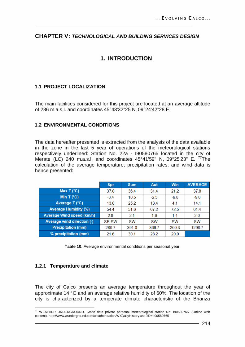
1.2 ENVIRONMENTAL CONDITIONS The data hereafter presented is extracted from the analysis of the data available in the zone in the last 5 year of operations of the meteorological stations respectively underlined: Station No. 22a - I90580765 located in the city of Merate (LC) 240 m.a.s.l, and coordinates 45°41'59" N, 09°25'23" E. 77The calculation of the average temperature, precipitation rates, and wind data is hence presented:

Table 10. Average environmental conditions per seasonal year.

1.2.1 Temperature and climate

The city of Calco presents an average temperature throughout the year of

approximate 14 C and an average relative humidity of 60%. The location of the city is characterized by a temperate climate characteristic of the Brianza

77

WEATHER UNDERGROUND. Storic data private personal meteorological station No. I90580765. (Online web

content). http://www.wunderground.com/weatherstation/WXDailyHistory.asp?ID= I90580765

http://www.wunderground.com/weatherstation/WXDailyHistory.asp?ID=%20I90580765

. . . E V O L V I N G C A L C O . . .

215

Lecchese, where winters trend to be rainy and to hold a temperature down to -

5C. Mid-seasons are wet (50% of year’s precipitation occurrence) and mild. In the last years during these seasons, the weather has been relatively temperate

presenting average temperatures of 13C as it can be seen in the table 0.2 During summer, day time is in average warm-hot with temperatures oscillating

among 20C and 25C, however nights are particularly fresh-cold presenting

temperatures close to 10C. summers are particularly also wet, presenting in average 30% of the total yearly precipitation.

Graphic 63. Maximum, minimum and average temperature.

Table 11. Seasonal and average yearly temperature and humidity conditions.

Spr Sum Aut Win AVERAGE

Max T (°C) 37.8 36.4 31.4 21.2 37.8

Min T (°C) -3.4 10.5 -2.5 -9.8 -9.8

Average T (°C) 13.8 25.2 13.4 4.1 14.1

Average Humidity (%) 54.4 51.6 67.2 72.5 61.4

. . . E V O L V I N G C A L C O . . .

216

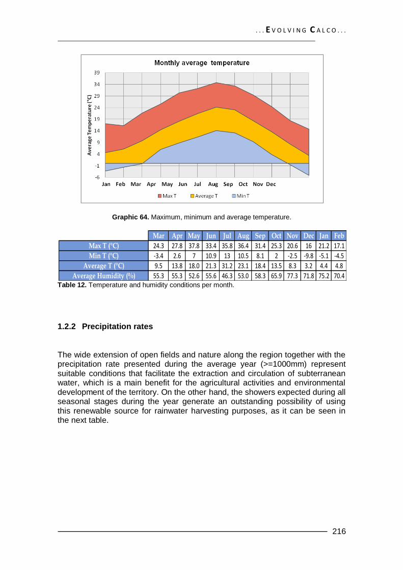
Graphic 64. Maximum, minimum and average temperature.

Table 12. Temperature and humidity conditions per month.

1.2.2 Precipitation rates

The wide extension of open fields and nature along the region together with the precipitation rate presented during the average year (>=1000mm) represent suitable conditions that facilitate the extraction and circulation of subterranean water, which is a main benefit for the agricultural activities and environmental development of the territory. On the other hand, the showers expected during all seasonal stages during the year generate an outstanding possibility of using this renewable source for rainwater harvesting purposes, as it can be seen in the next table.

Mar Apr May Jun Jul Aug Sep Oct Nov Dec Jan Feb

Max T (°C) 24.3 27.8 37.8 33.4 35.8 36.4 31.4 25.3 20.6 16 21.2 17.1

Min T (°C) -3.4 2.6 7 10.9 13 10.5 8.1 2 -2.5 -9.8 -5.1 -4.5

Average T (°C) 9.5 13.8 18.0 21.3 31.2 23.1 18.4 13.5 8.3 3.2 4.4 4.8

Average Humidity (%) 55.3 55.3 52.6 55.6 46.3 53.0 58.3 65.9 77.3 71.8 75.2 70.4

. . . E V O L V I N G C A L C O . . .

217

Graphic 65. Precipitation rate according to season.

Table 13. Seasonal and total precipitation rates.

Graphic 66. Precipitation rate according to month.

Table 14. Monthly precipitation rates.

0

50

100

150

200

250

300

350

400

450 P

reci

pit

atio

n (

mm

) Seasonal precipitation rates

Spring Summer Autumn Winter

Spr Sum Aut Win TOTAL

Precipitation (mm) 280.7 391.0 366.7 260.3 1298.7

% precipitation (mm) 21.6 30.1 28.2 20.0

0

20

40

60

80

100

120

140

160

180

Pre

cip

itat

ion

(m

m)

Monthly precipitation rates

Jan Feb Mar Apr May Jun Jul Aug Sep Oct Nov Dec


Precipitation (mm) 59.4 90.4 131.0 135.6 96.0 159.5 134.0 77.5 155.3 98.1 88.7 73.6

% precipitation (mm) 4.6 7.0 10.1 10.4 7.4 12.3 10.3 6.0 12.0 7.6 6.8 5.7

. . . E V O L V I N G C A L C O . . .

218

1.2.3 Wind characteristics

According to the data available, the region is characterized by the presence of ―light winds or calm wind condition‖ 78 (Beaufort scale) having an average velocity of 2.0 kmh and an orientation mainly towards South (S).

Graphic 67. Wind rose per season.

In the next list of tables and graphics it is represented the wind average velocities measured in the region at 25 and 50 m.a.t.l. 79

Table 15. Seasonal and year average wind velocities and orientation.

Table 16. Monthly wind velocities and orientation

1.2.4 Solar radiation

The monthly solar radiation parameters disposed for the area of the project are

calculated from the data base SAF-PVGIS of the European Joint Research

78

YEANG, Ken. Eco design: a manual for economical design. 2006. p. 213. 79

RICERCA SISTEMA ENERGETICFO. Atlante Eolico Italiano. 2011. (Online web content). http://atlanteeolico.rse-

web.it/viewer.htm

0

0.5

1

1.5

2

2.5

3 N

NE

E

SE

S

SW

W

NW

Wind velocities and orientation

Spring

Summer

Autum

Winter

Spr Sum Aut Win AVERAGE

Average Wind speed (km/h) 2.8 2.1 1.6 1.4 2.0

Average wind direction (-) SE-SW SW SW SW SW


Average Wind speed (km/h) 3.0 2.8 2.6 2.2 2.5 1.7 1.9 1.4 1.6 1.2 1.7 1.3

Average wind direction (-) S SSE SE SW SW SW SW SW SE SE SW SW

http://atlanteeolico.rse-web.it/viewer.htm


. . . E V O L V I N G C A L C O . . .

219

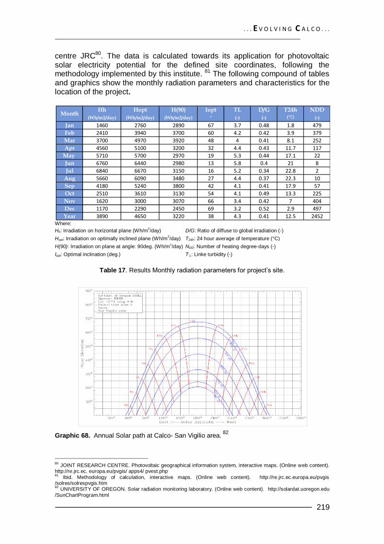
centre JRC80. The data is calculated towards its application for photovoltaic solar electricity potential for the defined site coordinates, following the methodology implemented by this institute. 81 The following compound of tables and graphics show the monthly radiation parameters and characteristics for the location of the project.

Where:

Hh: Irradiation on horizontal plane (Wh/m2/day) D/G: Ratio of diffuse to global irradiation (-)

Hopt: Irradiation on optimally inclined plane (Wh/m2/day) T24h: 24 hour average of temperature (°C)

H(90): Irradiation on plane at angle: 90deg. (Wh/m2/day) NDD: Number of heating degree-days (-)

Iopt: Optimal inclination (deg.) T L: Linke turbidity (-)

Table 17. Results Monthly radiation parameters for project’s site.

Graphic 68. Annual Solar path at Calco- San Vigilio area. 82

80

JOINT RESEARCH CENTRE. Photovoltaic geographical information system, interactive maps. (Online web content). http://re.jrc.ec. europa.eu/pvgis/ apps4/ pvest.php 81

Ibid. Methodology of calculation, interactive maps. (Online web content). http://re.jrc.ec.europa.eu/pvgis /solres/solrespvgis.htm 82

UNIVERSITY OF OREGON. Solar radiation monitoring laboratory. (Online web content). http://solardat.uoregon.edu

/SunChartProgram.html

Hh Hopt H(90) Iopt TL D/G T24h NDD

(Wh/m2/day) (Wh/m2/day) (Wh/m2/day) ° (-) (-) (°C) (-)

Jan 1460 2760 2890 67 3.7 0.48 1.8 479

Feb 2410 3940 3700 60 4.2 0.42 3.9 379

Mar 3700 4970 3920 48 4 0.41 8.1 252

Apr 4560 5100 3200 32 4.4 0.43 11.7 117

May 5710 5700 2970 19 5.3 0.44 17.1 22

Jun 6760 6440 2980 13 5.8 0.4 21 8

Jul 6840 6670 3150 16 5.2 0.34 22.8 2

Aug 5660 6090 3480 27 4.4 0.37 22.3 10

Sep 4180 5240 3800 42 4.1 0.41 17.9 57

Oct 2510 3610 3130 54 4.1 0.49 13.3 225

Nov 1620 3000 3070 66 3.4 0.42 7 404

Dec 1170 2290 2450 69 3.2 0.52 2.9 497

Year 3890 4650 3220 38 4.3 0.41 12.5 2452

Month

http://solardat.uoregon.edu/SunChartProgram.html


. . . E V O L V I N G C A L C O . . .

220

1.2.4.1 Irradiation on horizontal plane: This value is the monthly/yearly average of the sum of the solar radiation energy that hits one square meter in a horizontal plane in one day. This is measured in kWh/m2/day.

Graphic 69. Horizontal Irradiation, Optimal Irradiation, and Irradiation in a vertical surface

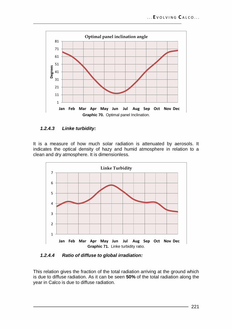
1.2.4.2 Optimal inclination angle:

It is the angle, in order to receive the maximum amount of solar energy on a flat plate facing south (I.e Solar panels). For this case the calculated optimal angle

is 38 for all the year, if the flat plate remains still along the year; however, this surface can be oriented month by month to the optimum angles described below.

1

1,001

2,001

3,001

4,001

5,001

6,001

7,001

8,001

Irra

dia

tio

n K

Wh

/m2/

day

Monthly Irradiation

Hh Hopt H(90)


. . . E V O L V I N G C A L C O . . .

221

Graphic 70. Optimal panel Inclination.

1.2.4.3 Linke turbidity:

It is a measure of how much solar radiation is attenuated by aerosols. It indicates the optical density of hazy and humid atmosphere in relation to a clean and dry atmosphere. It is dimensionless.

Graphic 71. Linke turbidity ratio.

1.2.4.4 Ratio of diffuse to global irradiation: This relation gives the fraction of the total radiation arriving at the ground which is due to diffuse radiation. As it can be seen 50% of the total radiation along the

year in Calco is due to diffuse radiation.

1

11

21

31

41

51

61

71

81

De

gre

es

Optimal panel inclination angle


1

2

3

4

5

6

7 Linke Turbidity


. . . E V O L V I N G C A L C O . . .

222

Graphic 72. Ratio of diffuse to global irradiation

1.2.4.5 Number of heating degree-days:

Considering an average comfort temperature of 18C for buildings, the heating degree-days are a measurement that reflects the demand of heat needed to satisfy this comfort temperature; besides, it can describe how cold the climate is. These values are calculated from daily average values of temperature reported in the table 3. As an example, if the average outside temperature for a day is 1 degree less

than the inside base temperature (18C), then it will be accumulated 1 degree day on that day and so on. The higher the number of degree days for the climate, the colder the climate it is., the ranges vary from 140 HDD per year (warm hot climate) up to 14000 per year (Cold climate) 83. Calco accumulates around 2500 heating days throughout the year.

83

NOAA satellite and information site. HDD locations united states. (Online web content).

http://www.ncdc.noaa.gov/oa/climate/online/ccd/nrmhdd.txt

0.0

0.1

0.2

0.3

0.4

0.5

0.6

0.7

0.8

0.9

1.0 Ratio of diffuse to global irradiation


. . . E V O L V I N G C A L C O . . .

223

Graphic 73. Number of heating degree-days per month.

1.3 POLICIES AND GUIDELINES The Energy plan of the Lecco province promotes the execution of projects and initiatives related to the use of new forms of energy in the province, but also directed to the general enhancement of the energy network in the territory. Following, there are listed the most important projects that directly or indirectly concern Calco’s territory and this thesis proposal.

- Promotion of wind farms of small size (maximum 20 kW) in areas of Alto Lario and Valsassina.

- Construction of small hydroelectric water systems for a power generation of not less than 0.5 MW. Saving between 3.500 and 4.500 MWh per year.

- Explore the possibility of use of biomass energy from forests existent along the territory.

- Use of solar energy to produce hot water for public buildings or of public use.

- Use of the governmental economical support system ―Conto energia‖ for the implementation of photovoltaic panels, Expected future application of the expired regulation.

0.0

100.0

200.0

300.0

400.0

500.0

600.0 Number heating degree - days


. . . E V O L V I N G C A L C O . . .

224

2 INFORMATION ANALYSIS

2.1 SWOT ANALYSIS

STRENGHTS

▪ Allowance to provide free orientation of the main building and facilities. ▪ Temperate climate, does not present extreme temperatures variations

among seasons. ▪ Precipitation rates suitable for rainwater harvesting purposes.

WEAKNESSES

▪ 90% of the territory uses nowadays metanol gas, 6% regular fuel vs. 1% coming from renewable sources for mainly heating purposes. 84

▪ Main current electrical consumption in residential buildings due to illumination (15%), refrigeration systems (19%) and use of Audio/video devices (17%).85

▪ Main current electrical consumption in public buildings due to illumination (35%), AHVC (18%) and use of Audio/video devices (12%).86

▪ Average Low annual wind velocities (<3m/s) measured at 25m a.t.l and 50m a.t.l, make unpractical the use of wind power.

OPPORTUNITIES

▪ Promotion to construct small hydroelectric water systems applied to existing network of water supply.

▪ 30% of Calco’s area is composed by forest87, the policies regarding exploration of use of Biomass from these areas is considered an opportunity to apply this renewable source of energy in the project.

▪ Governmental economical support for the implementation of Photovoltaic panels.

84

PROVINCIA DI LECCO. Piano Energetico Territoriale Provinciale(PETP): VolIIscenari. 2008. p. 33. 85



PROVINCIA DI LECCO. Piano Energetico Territoriale Provinciale(PETP): VolIIscenari. 2008. p. 92.

. . . E V O L V I N G C A L C O . . .

225

THREATS

▪ The not inclusion of Calco’s territory inside the plan of wind Energy

promotion. ▪ Goal to guarantee 50% coverage of the total consumption due to water

heating in all the year using solar heating systems.

. . . E V O L V I N G C A L C O . . .

226

3 STRATEGY

3.1 RENEWABLE-ENERGY TECHNOLOGIES AND ENERGY EFFICIENCY MEASURES

3.1.1 Small Hydropower generation:

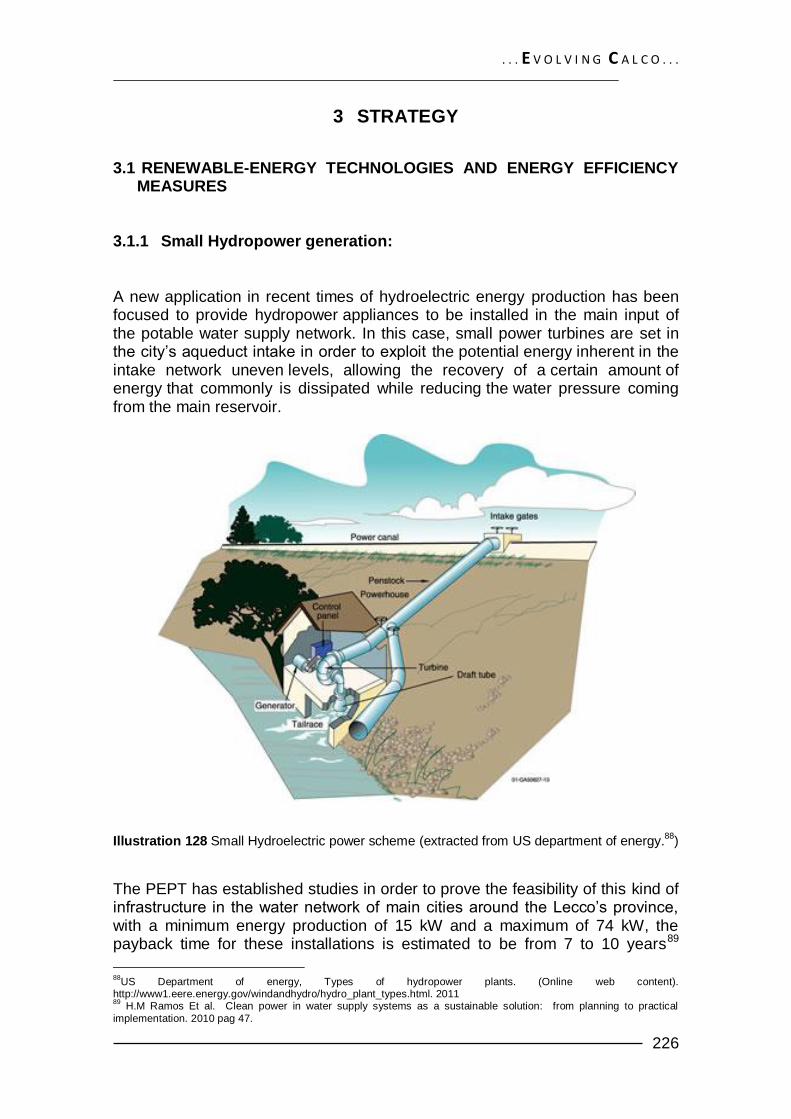
A new application in recent times of hydroelectric energy production has been focused to provide hydropower appliances to be installed in the main input of the potable water supply network. In this case, small power turbines are set in the city’s aqueduct intake in order to exploit the potential energy inherent in the intake network uneven levels, allowing the recovery of a certain amount of energy that commonly is dissipated while reducing the water pressure coming from the main reservoir.

Illustration 128 Small Hydroelectric power scheme (extracted from US department of energy.88

)

The PEPT has established studies in order to prove the feasibility of this kind of infrastructure in the water network of main cities around the Lecco’s province, with a minimum energy production of 15 kW and a maximum of 74 kW, the payback time for these installations is estimated to be from 7 to 10 years89

88

US Department of energy, Types of hydropower plants. (Online web content). http://www1.eere.energy.gov/windandhydro/hydro_plant_types.html. 2011 89

H.M Ramos Et al. Clean power in water supply systems as a sustainable solution: from planning to practical

implementation. 2010 pag 47.

. . . E V O L V I N G C A L C O . . .

227

depending on the estimated production of energy which ranges from 127 to 637 MWh/year in individual cities. 90 If we consider a mean value (360 MW/year) for Calco’s energy production from this energy source, but also mean values of projected electric consumption 0.9MW/inhb91 and population growth of 5132 inhb92 by the year 2020, it can be calculated in average the percentage of energy that a hydropower plant located in the municipality would be able to meet with respect to the consumption in the residential sector of the town itself. As a result a possible small hydropower plant located in Calco can satisfy the 8% of the electric demand of the resident population by 2020, when the total investment payback will be generated already. This value is given only for projection matters, and it does not demonstrate a real quantity of the energy intake to be generated from Calco’s possible potable water network system. 3.1.2 Biomass production

The implementation of Biomass use in the zone of Calco, lies in the idea of recollection, processing (chipping/pelleting) and supply of residues derivative of forests and agricultural fields, such as fallen leafs, cut down stems due to coppicing93 and natural tree life cycle, dried tree branches etc… residues which are considered not only to be a potential source of energy, but also to be responsible of a probable risk of fire.

Illustration 129 Biomass power generation and coppicing schemes (extracted from ISIS94) The wide extension of agricultural and forest areas disposed inside and at the vicinity of the city as it is presented in the ANNEX 1 PTCP brief, makes Calco a

90

PROVINCIA DI LECCO. Piano Energetico Territoriale Provinciale(PETP): VolIIscenari. 2008. p. 120-121 91

Ibid. Piano Energetico Territoriale Provinciale(PETP): VolIIscenari. 2008. p. 120-121 92

ISAT. Calco 2020 demographic measurement http://demo.istat.it/bil2010/index02_e.html 93

Copicing: is a traditional method of woodland management which takes advantage of the fact that many trees make new growth from the stump or roots if cut down. 94

ISIS Arturo Malignani Udine. Alternative power sources at different latitudes in Europe (Online web content).

http://www.malignani.ud.it/webenis/northwind-southsun/power/Biomass.htm

http://demo.istat.it/bil2010/index02_e.html

http://en.wikipedia.org/wiki/Woodland_management

http://en.wikipedia.org/wiki/Tree

. . . E V O L V I N G C A L C O . . .

228

suitable place for the implementation of action plans that lead in the future, to the use of Biomass as a main source of energy for combined heat and power applications CHP (other outcomes such as fertilizers, concrete fillers, electrical energy can be considered), as well as an alternative for economical growth in the region. The province of Lecco establishes that around 80%95 of the area of the forests in the region is constituted by shoots or suckers (kind of tree capable to be specially subjected to Coppicing).

Due to the aspects before presented, the Lecco province promotes redundantly the inclusion on local systems of supply and consumption of residual Biomass aimed to the production of small-medium size heat network for public & private facilities, and small industries. However systems for direct supply of chipping/pelleting for domestic internal heating purposes should be considered as part of the general approach of this source of energy. It has to be taken into consideration that the province of Lecco has supported feasibility studies (€ 50.000 for each potential locality) of this kind of projects in the region.96

Illustration 130. Calco’s north-oriental forest and agricultural fields

3.1.3 Solar photovoltaic energy

Solar energy can be converted into electric energy by the use of photovoltaic cells’ systems. These systems can be designed and developed to satisfy the needs and requirements of the operations given by the building or facility. The power generated from this type of energy can be used to satisfy internal demand as well as external demand (See scheme below).

95

PROVINCIA DI LECCO. Piano Energetico Territoriale Provinciale(PETP): VolII scenari. 2008. p. 94 96

Ibid. Piano Energetico Territoriale Provinciale(PETP): VolII scenari. 2008. p. 89

http://en.wikipedia.org/wiki/Euro_sign

. . . E V O L V I N G C A L C O . . .

229

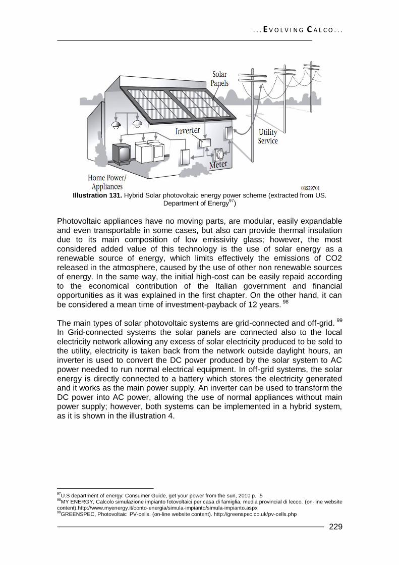
Illustration 131. Hybrid Solar photovoltaic energy power scheme (extracted from US.

Department of Energy97

)

Photovoltaic appliances have no moving parts, are modular, easily expandable and even transportable in some cases, but also can provide thermal insulation due to its main composition of low emissivity glass; however, the most considered added value of this technology is the use of solar energy as a renewable source of energy, which limits effectively the emissions of CO2 released in the atmosphere, caused by the use of other non renewable sources of energy. In the same way, the initial high-cost can be easily repaid according to the economical contribution of the Italian government and financial opportunities as it was explained in the first chapter. On the other hand, it can be considered a mean time of investment-payback of 12 years. 98 The main types of solar photovoltaic systems are grid-connected and off-grid. 99 In Grid-connected systems the solar panels are connected also to the local electricity network allowing any excess of solar electricity produced to be sold to the utility, electricity is taken back from the network outside daylight hours, an inverter is used to convert the DC power produced by the solar system to AC power needed to run normal electrical equipment. In off-grid systems, the solar energy is directly connected to a battery which stores the electricity generated and it works as the main power supply. An inverter can be used to transform the DC power into AC power, allowing the use of normal appliances without main power supply; however, both systems can be implemented in a hybrid system, as it is shown in the illustration 4.

97

U.S department of energy: Consumer Guide, get your power from the sun, 2010 p. 5 98

MY ENERGY, Calcolo simulazione impianto fotovoltaici per casa di famiglia, media provincial di lecco. (on-line website content).http://www.myenergy.it/conto-energia/simula-impianto/simula-impianto.aspx 99

GREENSPEC, Photovoltaic PV-cells. (on-line website content). http://greenspec.co.uk/pv-cells.php

http://www.myenergy.it/conto-energia/simula-impianto/simula-impianto.aspx

. . . E V O L V I N G C A L C O . . .

230

3.1.4 Geothermal energy systems

The Ground Source Heat Pump (GSHP) systems work by extracting heat from de ground during winter seasons, and reciprocally, by releasing heat during summer into the ground, taking advantage of the almost constant temperature

of the soil during the year (12C for Milan - Italy) 100. One type of systems is the closed Loop systems: These systems circulate a mixture of water and antifreeze liquid throughout a loop of pipe buried in the ground; the loop absorbs heat from the soil and transports it to a heat exchanger powered by an electric pump and compressor.

Illustration 132. GSHP closed loop systems scheme (extracted from US department of energy

101)

The other main category of ground source heating pump systems is the so called open loop system. It uses well or surface body water as the heat exchange fluid that circulates directly through the GHP system. Once it has circulated through the system, the water returns to the ground through the well, a recharge well, or surface discharge. This option is obviously practical only where there is an adequate supply of relatively clean water102, which is assumed to be the San Vigilio area in Calco (project area).

Illustration 133. GSHP Open loop systems scheme (extracted from US department of

energy103

)

100

U.S department of energy: Consumer Guide, get your energy from the sun, 2001, p. 4, 101

US. DEPARTMENT OF ENERGY. Types of geothermal Heat pump system. (on-line website content). http://www.energysavers.gov/your_home/space_heating_cooling/index.cfm/mytopic=12650.2011 102

Ibid, Types of geothermal Heat pump system. (on-line website content). http://www.energysavers.gov/your_home/space_heating_cooling/index.cfm/mytopic=12650.2011 103

Ibid, Types of geothermal Heat pump system. (on-line website content).

http://www.energysavers.gov/your_home/space_heating_cooling/index.cfm/mytopic=12650.2011

. . . E V O L V I N G C A L C O . . .

231

Although there is no geothermal energy plan contemplated in the PETP, the use of this technology can be a complementary source of energy to the solar water heating systems, in the production of hot water and cold water for the air conditioning units to be supplied into the project. On the other hand the sources of energy needed to activate the pumping systems can be extracted from solar photovoltaic energy; by combining this approach it can be achieved a 400% of efficiency of the GSHP, generating 0.00 CO2 emissions. 104

3.1.5 Rain water recollection and application to services.

Rainwater has been during centuries one of the most common sources of water needed to meet agricultural requirements, and in some case, potable water as well. Most rainwater collection systems are designed to capture rainwater from the roofs of buildings; however systems of recollection of rainwater once it has been drained through natural surfaces are considered also. The water is then transported through gutters and other pipes into cisterns or tanks, where it is stored until needed. The water collected can be used for irrigation, laundry, hygiene, or even potable water, depending upon the materials used and the treatments undertaken. In most cases when the water is not treated, the rain water is used for irrigation, toilets, flushing water, and in some limited cases for laundry.

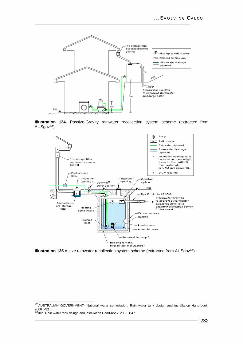
The recollected water can supply different fixtures in the building in two ways. A passive way can take advantage of gravity and head of pressure obtained by locating the storage tank in a higher level from the fixtures to be used; this system has as main disadvantage the need of continuous and elevated collocation of the storage tanks, which can be constrained according to the general aspect, space conditions, configuration of the building, and main water supply network level (which provides a backup for the water supply).

The other type of systems store collected water in a ground tank, from which it is pumped back to the fixtures for its later use. The main disadvantages of this systems is the need of electricity for pumping (which can be satisfied by PV solar panels) and the need of a second storage tank in each fixture (specially toilets) that can maintain the needed flux of water.

104

GREEN SPEC, Ground source heating pumps. (on-line website content ). http://greenspec.co.uk /ground-source-

heat-pumps.php

. . . E V O L V I N G C A L C O . . .

232

Illustration 134. Passive-Gravity rainwater recollection system scheme (extracted from AUSgov105)

Illustration 135 Active rainwater recollection system scheme (extracted from AUSgov106)

105

AUSTRALIAN GOVERNMENT- National water commission. Rain water tank design and installation Hand-book. 2008. P21 106

Ibid Rain water tank design and installation Hand-book. 2008. P47

. . . E V O L V I N G C A L C O . . .

233

3.1.6 Appliances for electrical consumption reduction.

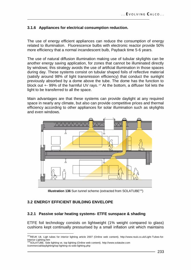
The use of energy efficient appliances can reduce the consumption of energy related to illumination. Fluorescence bulbs with electronic reactor provide 50% more efficiency that a normal incandescent bulb, Payback time 5-6 years. The use of natural diffusion illumination making use of tubular skylights can be another energy saving application, for zones that cannot be illuminated directly by windows; this strategy avoids the use of artificial illumination in those spaces during day. These systems consist on tubular shaped foils of reflective material (satisfy around 98% of light transmission efficiency) that conduct the sunlight previously absorbed by a dome above the tube. The dome has the function to block out +- 99% of the harmful UV rays. 107

At the bottom, a diffuser foil lets the light to be transferred to all the space. Main advantages are that these systems can provide daylight at any required space in nearly any climate, but also can provide competitive prices and thermal efficiency according to other appliances for solar illumination such as skylights and even windows.

Illustration 136 Sun tunnel scheme (extracted from SOLATUBE108)

3.2 ENERGY EFFICIENT BUILDING ENVELOPE

3.2.1 Passive solar heating systems- ETFE sunspace & shading ETFE foil technology consists on lightweight (1% weight compared to glass) cushions kept continually pressurised by a small inflation unit which maintains

107

REUK Uk. Ligh tubes for interior lighting article 2007 (Online web content). http://www.reuk.co.uk/Light-Tubes-for-Interior-Lighting.htm 108

SOLATUBE. Side lighting vs. top lighting (Online web content). http://www.solatube.com

/commercial/daylighting/top-lighting-vs-side-lighting.php

http://www.solatube.com/

. . . E V O L V I N G C A L C O . . .

234

the pressure at approx. 220 Pa and gives the compound of two or more foils inside the cushions a structural stability while providing also high efficient

insulation performance (3 foils, U = 1.96 W*m2/K)109

Illustration 137. sun shading system system. Open and closed configuration (extracted from VECTORFOILTEC

110)

High technological advanced systems can provide full controlled shading by means of alteration between the pressure of the foils and the pattern of them, as it can be shown in the next figure. Basically a foil in between the two chambers can be blown to the top of the surface, creating an enclosed penetration of sun rays, according by the pattern inked into its surface; in order to let the light go in, the foil is unpressurised.

Illustration 138 Configuration of three foils with sun shading system foil (extracted from VECTORFOILTEC

111)

A classical system is composed of a series of pneumatic cushions made up of between two and five layers of a modified copolymer called Ethylene Tetra

109

VECTORFOILTEC. Texlon technical specifications. http://www.vector-foiltec.com/cms /gb/ technical/ randd.php.

2011. 110

VECTORFOILTEC. Variable skins. http://www.vector-foiltec.com/cms/gb/technical /variableskins.php 111

VECTORFOILTEC. Texlon technical specifications. http://www.vector-foiltec.com/cms /gb/ technical/ randd.php.

2011.

. . . E V O L V I N G C A L C O . . .

235

Flouro Ethylene (ETFE), is supported by basic circular or extruded aluminum profiles that can be connected to any common structural system made out of cables or steel profiles.

Illustration 139 Typical structural system and connections of the system (extracted from ARCHITEN112)

The use of a secondary ETFE skin will generate a controlled green-house effect on winter, while a free release of internal loads on summer, when this secondary façade can be wide open. (Indirect diffusion gain) or some openings can generate the natural ventilation required.

Illustration 140 Ventilation systems for ETFE pneumatic cushions (extracted from VECTORFOILTEC

113)

By effectively adding another layer to the building envelope, the sunspace becomes a thermal buffer of air within a cavity wall. A further effect of the sunspace is to shelter the envelope from wind chill and rain which are factors that affect the area of the project precisely in North-south direction where wind permanently blows.

112

ARCHITEN. ETFE foil: A guide to design. 2011 p 14. 113

VECTORFOILTEC. Ventilation systems. http://www.vector-foiltec.com/cms/gb /technical/ ventilation.php

. . . E V O L V I N G C A L C O . . .

236

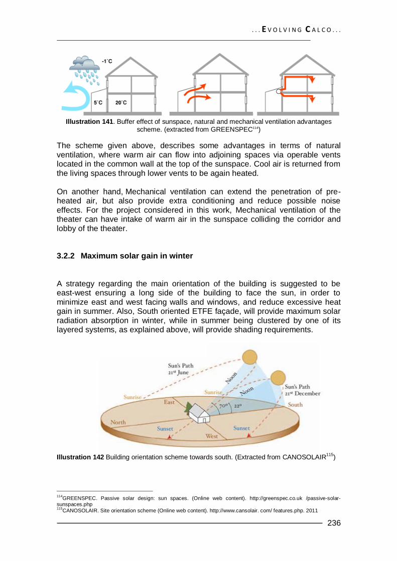
Illustration 141. Buffer effect of sunspace, natural and mechanical ventilation advantages

scheme. (extracted from GREENSPEC114)

The scheme given above, describes some advantages in terms of natural ventilation, where warm air can flow into adjoining spaces via operable vents located in the common wall at the top of the sunspace. Cool air is returned from the living spaces through lower vents to be again heated. On another hand, Mechanical ventilation can extend the penetration of pre-heated air, but also provide extra conditioning and reduce possible noise effects. For the project considered in this work, Mechanical ventilation of the theater can have intake of warm air in the sunspace colliding the corridor and lobby of the theater. 3.2.2 Maximum solar gain in winter

A strategy regarding the main orientation of the building is suggested to be east-west ensuring a long side of the building to face the sun, in order to minimize east and west facing walls and windows, and reduce excessive heat gain in summer. Also, South oriented ETFE façade, will provide maximum solar radiation absorption in winter, while in summer being clustered by one of its layered systems, as explained above, will provide shading requirements.

Illustration 142 Building orientation scheme towards south. (Extracted from CANOSOLAIR

115)

114

GREENSPEC. Passive solar design: sun spaces. (Online web content). http://greenspec.co.uk /passive-solar-sunspaces.php 115

CANOSOLAIR. Site orientation scheme (Online web content). http://www.cansolair. com/ features.php. 2011

. . . E V O L V I N G C A L C O . . .

237

3.2.3 Efficient ventilation

Efficient ventilation in the building can be provided by using the advantages of both natural and mechanical ventilation. Due to the need of regulation of air quality, sound quality and possible draughts in the theater/auditorium, the best solution is to provide mechanical ventilation with heat-recovery systems, and probable air tightness; in the same way, the mechanical system to be proposed, can take advantage of solar air heating collectors and/or ground water pump, technology that has been newly implemented in commercial and industrial uses as it was described before.

Natural ventilation is generally suitable only for selective areas such as lobbies, staircases and toilets, which can have operable windows or air gaps to the exterior. Due to the one-floor configuration and its height, it becomes not useful the use of stack effect, which can generate thermal bridges with low effect in ventilation performance, as a result its application is limited to bathrooms and restaurant kitchens. However a crucial strategy has been chosen in order to provide the best performance of the building in terms of HAVC system efficiency, points that will be further discussed in the chapter 6. HVAC SYSTEMS.

3.2.4 Air tightness

Building an airtight thermal consists on arranging the structure of the building in order to avoid infiltration or too high losses of latent heat during winter. Satisfying air tightness ensures the efficacy of the mechanical ventilation system chosen for the project to control the humidity in the environment and satisfy easily the needs of thermal comfort while the moisture is kept away of causing deterioration of the structure. 3.2.5 Super Insulation In zones with relative low temperatures such as the north of Italy and central Europe, the R-Values set on external walls, slab foundation and roofs ranges among 38 and 52 reduces the heating losses and gains throughout the seasons, keeping the house at a balanced temperature and humidity level with a lower use of energy. 3.2.6 Thermal Bridging Reduction In addition to the use of high insulation levels, the removal of thermal bridges from inside to the outside of the house would avoid the heat flow through the least resistance paths (wool, metal, etc.), empowering the insulation effect. This thermal bridging reduction is avoided by considering a total a construction detailing in which the insulation path can enclose entirely all the building envelope avoiding insulation offsets in joints and connections.

. . . E V O L V I N G C A L C O . . .

238

3.3 ACUSTICAL SUITABLE PERFORMANCE Another topic that the theater/auditorium in concern should satisfy is level of acoustical performance that can be acquired by following simple but effective strategies in terms of internal shape, materials, and distribution. 116 The quality of sound for a theater can be given by three main aspects, sonority, reflection and reverberation time. 3.3.1 Criteria for direct sound generation It is suitable to have any receptor to a distance no more than 20 m from the source in order to avoid a misinterpretation of the message, however, this fact depends on the attenuation given by the room or the amplification of the source. 3.3.2 Criteria for first reflection generation Even when there was made a careful choice of the materials in order to obtain the recommended values of reverberation time for any space, it does not guarantee the complete the recognition of the message and an optimum sonority in all the points of the place. It s needed to avoid certain phenomena such as echo, flutter echo and focalization with the implementation of practical shapes. In terms of shape, the sonority and a graceful first reflection should be satisfied in order to avoid certain phenomena to be discussed here after;

Illustration 143 Ceiling and wall convex and reflective surfaces (extracted from CARRION117)

3.3.3 Echo reduction Every sound reflection that arrives to a receptor in between the first 50 ms after the arrival of the direct sound is recognized by the human ear as a single sound. When the sound is emitted from any oral source the existence of those reflections help to improve the comprehension of the sound; on the other hand, the appearance of certain reflections of sound with a delay higher than 50ms,

116

CARRION Antoni. Diseño acústico de espacios architectonicos. 1998. P. 137 117

Ibid. Diseño acústico de espacios architectonicos. 1998. p. 198-201

. . . E V O L V I N G C A L C O . . .

239

recreates a repetition of the first sound emitted called echo. Two main solutions can be given to avoid echo.

a. Use absorption material or Helmotz selective absorption type in the surfaces with a proportion of not more than 10% of the total area covered. Further absorption material could affect the reverberation time of the room.

b. Use convex surfaces. c. Use of tilted surfaces.

Illustration 144 Solutions to avoid echo (extracted from CARRION118)

3.3.4 Flutter Echo reduction The flutter echo consists on the multiple repetitions in a small period of time of a sound generated by any source in an space enclosed by mainly highly reflective and smooth. This phenomenon can be prevented by avoiding de use of large reflecting parallel walls; a reflective wall is composed mainly by sound reflective material such as wood.

The solution relies on either incline one of the walls at least 5 inclined, or a less effective alternative, absorption material. 3.3.5 Focalization In cases when the surfaces are concave such as domes or circular plans, the energy emitted by a source will be focalized into a single point, forming unbalance in the level of sound reception between different points with of the room. The solution is to avoid these circular shapes in walls and ceilings.

118

Ibid. Diseño acústico de espacios architectonicos. 1998. p. 209

. . . E V O L V I N G C A L C O . . .

240

4 THERMAL DESIGN OF BUILDING ENVELOPE

4.1 TECHNICAL ENVIRONMENTAL DATA The present environmental data is analyzed in order to obtain the conditions at which the system will run during the average summer and winter season.

Table 18. Technical environmental data Calco –Lecco province (extracted from UNI13049)

Table 19. Materials thermal and permeability properties

. . . E V O L V I N G C A L C O . . .

241

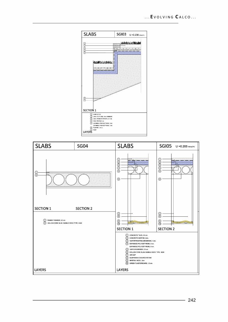
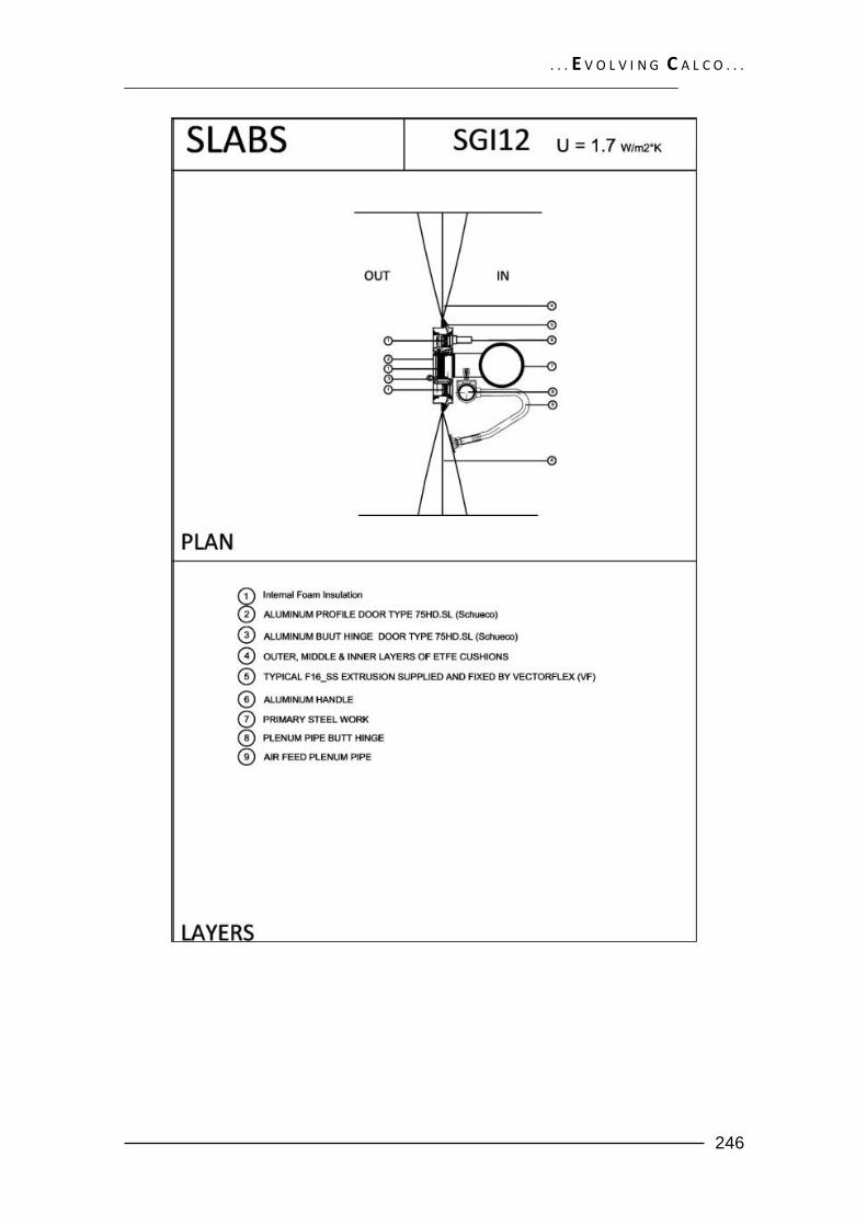
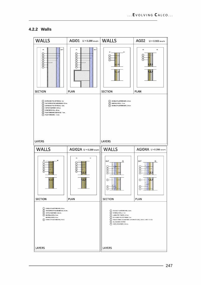
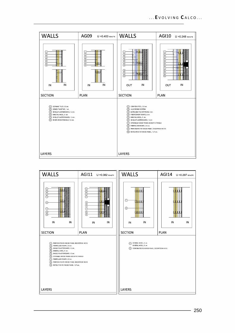
4.2 TECHNOLOGICAL CHOICES A detail abacus was created compiling all the different material solutions and layers for the range of walls and slabs proposed as technological solution in our project, taking into account into the design of the thermal efficient envelope. Based on these we started the calculations of the U values for each one of the elements and its components.

4.2.1 Slabs

. . . E V O L V I N G C A L C O . . .

242

. . . E V O L V I N G C A L C O . . .

243

. . . E V O L V I N G C A L C O . . .

244

. . . E V O L V I N G C A L C O . . .

245

. . . E V O L V I N G C A L C O . . .

246

. . . E V O L V I N G C A L C O . . .

247

4.2.2 Walls

. . . E V O L V I N G C A L C O . . .

248

. . . E V O L V I N G C A L C O . . .

249

. . . E V O L V I N G C A L C O . . .

250

. . . E V O L V I N G C A L C O . . .

251

4.3 METHODOLOGY The methodology for the analysis of the building envelope is done by assessing the performance of the building during winter and summer in terms of energy needs for heating or cooling. The boundary of the building has been designed in order to offer the energy efficiency needed to satisfy the requirements of a zero foot print building, (less energy consumption, higher the possibilities to obtain the highest part of the energy from renewable sources exclusively). In order to assess numerically the performance of the building envelope, the considerations and guidelines of the standard UNI 10351 – and ISO 1007-1:2007 are carried out as follows:

4.4 CONDENSATION RISK: U-VALUES AND GLAZER DIAGRAM. The condensation risk measures numerically the direct probability in which a multilayered system can suffer from interstitial condensation, phenomena that leads commonly to accumulation of high amounts of water carried by the air. The phenomenon has to be avoided in order to guarantee the reliability of the components used during the entire service life of the structure, which can be compromised by biological growth, efflorescence and general deterioration of the layer or compound of layers in which this phenomenon can happen.

. . . E V O L V I N G C A L C O . . .

252

When condensation occurs the only possibility to avoid it (other than changing the composition of the multilayered component) is to employ a Vapor barrier in the layer where condensation is more likely to occur. As a result, the next calculation for each type of wall, and slab is generated aiming to know if the inclusion of a vapor barrier is needed or not. In numerical terms, the need of vapor barrier can be obtained by making a comparison between the diagram of saturation pressure and vapor pressure (Glaser diagram) at every intersection between parallel layers for a flux of thermal energy, both during winter and during summer. Steps:

1. The temperatures at each interface of the wall can be calculated using the next formula:

Where:

Ti = Temperature of the interface i. C Ti-1 = Temperature of the precedent interface in the flux direction. Tin = Temperature inside. Tout = Temperature Outside. Ri = Thermal resistance of the interface i RT = Total thermal resistance of the component

2. By knowing the temperatures through each wall, saturation pressure can be approximated to:

3. The vapor pressure at each interface can be calculated from the next formula:

Where: Ti = Vapor pressure at the interface i Ti-1 = Vapor pressure of the precedent interface in the flux direction. Tin = Vapor pressure inside. Tout = Vapor pressure Outside. Ri = Vapor flow resistance of the interface i RT = Vapor flow resistance of the component

The ANNEX 2 shows the calculation and results of the condensation risk for each type of wall and then the inclusion of a water vapor barrier according to

. . . E V O L V I N G C A L C O . . .

253

the outcome of the analysis can be seen in the list of abacus presented above. However an example of the analysis developed is hereafter presented:

Illustration 145 Slab SG-02 Condensation risk analysis

4.5 THERMAL COMFORT ASSESSMENT In order to understand the comfort levels that could be achieved at our spaces we analyzed the mean radiant temperatures for 5 of the main spaces in our project with the aim of understanding what the overall thermal sensation in our building would be considering the different layers of the envelope. We also considered calculating the buffer area in the entrance of the theater to understand the effect the radiation of the different surfaces affecting the space even though we understand the comfort levels for this kind of spaces are more flexible due to the fact that it is a transition zone. The results and process of

. . . E V O L V I N G C A L C O . . .

254

these calculations are plotted in the tables following, which give as a result acceptable comfort levels in all the spaces except, of course for the buffer area. The main 5 Spaces studied were: The Bar and its Kitchen, the restaurant, the exposition gallery and the theater, each for a different specific location and situation (sitting or standing). The process we followed to assess the effects of radiation in terms of the mean radiant temperature for each space were as follows: In every room of the building studied we calculated:

Where Ti is the surface indoor temperatures of the enclosure surfaces and Fvi are the shape factors of the surfaces with respect to a specific point within the space. The calculation of the shape factors are done considering the division of the surfaces with respect to the subject inside the space. Depending of different cases (whether the user is standing or sitting different tables are available for the calculations of these factors through the formula:

Considering the values are taken from the relationship with the reference table where they can be calculated as:

The view factors can then be summed up to obtain the total Mean radiant temperature. After this we can calculate the operating temperature which will indicate us the thermal comfort level in the space. Operative temperature is approximated as the average of the dry bulb temperature and the mean radiant temperature. If the operative temperature is greater than 19 degrees there is an acceptable thermal comfort level.119 For the sake of simplicity it has been studied particular spaces that are assumed to drive the comfort conditions in all the building area. The results of the analysis and zones are here presented:

119

MASERA GABRIELE. Thermal Comfort Presentation. (Available online) http://corsi.metid.polimi.it/col/data/contenuti/base_gruppi/078263_5597/allegati/LS01c%20TD%20-

%20thermal%20comfort.pdf. 2010

. . . E V O L V I N G C A L C O . . .

255

Table 20 summary of results of comfort assessment

The next illustration shows the results of the analysis for one particular case as an example of the process realized; however the ANNEX 4 shows the entire calculation tables and results for all the cases analyzed. Surface

. . . E V O L V I N G C A L C O . . .

256

Results

Illustration 146 Kitchen Bar – Viewer in the Middle and Standing – thermal comfort analysis

. . . E V O L V I N G C A L C O . . .

257

5 LIGHTING DESIGN

5.1 INTRODUCTION:

“The objective of architectural lighting design is to obtain sufficient light for the purposes of the building, balancing factors of initial and operating cost, appearance, and energy efficiency”120

Lighting design is an important aspect in the technological characteristics of a building. It requires consideration of the amount of functional light provided, the energy consumed, as well as the aesthetic impact supplied by the lighting system. Some buildings are primarily concerned with providing the appropriate amount of light for the associated task (such as sports facilities). Some buildings are primarily concerned with saving money through the energy efficiency of the lighting system (office and commercial buildings). Other buildings are primarily concerned with enhancing the appearance and emotional impact of architecture through lighting systems (theatres). Therefore, it is important that the lighting design process to be balanced with both, the artistic application of light as a medium in our built environment, as well as the impacts of day-lighting systems and be integrated with them in order to reach a holistic design/energy conservation approach. This methodology of analysis employed in this chapter aims to simulate the sun path in the most important days in the four seasons of the year and its effect in terms of shading on the project building masses and their surroundings. This allows the understanding of the level of sunlight accessibility throughout the whole project and whether the orientation is well fixed or not.

5.2 SOLAR LOCAL PATH:

By using the environmental and geo-reference data of the Wheater station Bergamo-orio al serio, the program Ecotect generates the following sun-paths around the project masses during winter and during summer.

120

GARY R. Steffy Architectural lighting design. 2002. p 24.

. . . E V O L V I N G C A L C O . . .

258

WINTER SOLSTICE: DECEMBER 21 Local Correction: -19.1 mins Equation of Time: 2.1 mins

Sunrise: 08:04 Sunset: 16:33 Declination: -23.5°

Illustration 147 Graphical representation of the solar path in winter

Table 21 Winter Solar path and time

Summer looks like the usual days, but rather short in terms of time. The day with the lowest sun altitude is the same as that of the whole year; this corresponds to 20.8° at 12:30p.m.

. . . E V O L V I N G C A L C O . . .

259

INVERNAL EQUINOX: March 21 Local Correction: -28.4 mins Equation of Time: -7.2 mins

Sunrise: 06:29 Sunset: 18:27 Declination: -0.3°

Illustration 148 Graphical Representation of the Solar Path in spring

Table 22 Spring Solar path and time

. . . E V O L V I N G C A L C O . . .

260

The spring equinox works as a transitional period between winter and summer. In this regard it is noted that the highest point of the sun in the sky is: 44.0 °; at 12:30p.m.

SUMMER SOLSTICE: JUNE 21 Local Correction: -22.8 mins Equation of Time: -1.6 mins

Sunrise: 04:37 Sunset: 20:08 Declination: 23.4°

Illustration 149 Graphical Representation of the Solar Path in summer

Table 23 Summer Solar Path and time

. . . E V O L V I N G C A L C O . . .

261

Summer looks like the usual days, but rather long in terms of time. The day with the highest sun altitude is the same as that of the whole year; this corresponds to 67.7° at 12:30p.m.

AUTUMNAL EQUINOX: SEPTEMBER 21 Local Correction: -14.3 mins Equation of Time: 6.9 mins

Sunrise: 06:10 Sunset: 18:18 Declination: 1.0°

Illustration 150 Graphical Representation of the Solar Path in autumn

Table 24 Autumn Solar Path and time

. . . E V O L V I N G C A L C O . . .

262

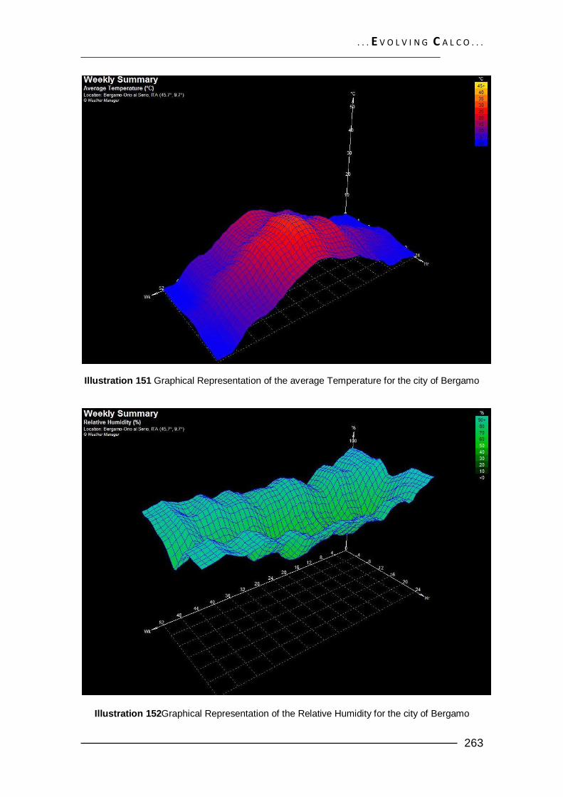
The autumnal equinox has values substantially equal to those of spring days. The discrepancies between the two days are somehow little. The altitude of the Day is: 45.2° at 12:00 & 12:30. CONCLUSION (NOTE): From the lighting simulation of the project area and the context around it, it’s notable that the building has good access to sunlight in each of the cases seen. Also, the orientation of the main openings (glazed areas) is well positioned (towards the south). However, spaces such as the bars and restaurants depths could lead to problems in the lighting levels within the spaces. The daylight factor analysis will host different alternatives for solving such a potential issue in the next part of this chapter. The shadows reach the context in later times of the day. The shape of the building and its inclusion in the site identifies two main fronts; South and Western facades. The eastern part is covered with earth, since the mass is emerging from it due to the difference in levels between the San Vigilio church and the park level; the same goes for the North façade. Another fact to consider is the analysis of local weather conditions that define the average situation of the local cloud. In this case, we used the data for the city of Milano, since the data for Calco or Bergamo wasn’t available, and the differences in the results are not expected to be of major significance. All the other results are based on the weather data of the city of Bergamo.

. . . E V O L V I N G C A L C O . . .

263

Illustration 151 Graphical Representation of the average Temperature for the city of Bergamo

Illustration 152Graphical Representation of the Relative Humidity for the city of Bergamo

. . . E V O L V I N G C A L C O . . .

264

Illustration 153 Graphical Representation of the average Cloud Cover for the city of Milano

It is obvious that a clear day is not on the agenda and that the average trend of the weather, settles down on a condition of partial cloudiness.

5.3 NATURAL LIGHTING ANALYSIS The management of the natural light is designed to optimize its use to obtain better living conditions inside the environment. In addition to its use may reduce the artificial light in terms of quantity and time to obtain the benefits of economic power consumption. In our case, due to the size of the south windows, and in order to obtain the maximum glass area clean, we tried the horizontal development in accordance with the will to give to the prospectus in horizontal planes integrated within the window (Okalux glazing systems) above the base on the south, west and east façade; some parts of the south and west façade are made of ETFE, which is difficult to model with their characteristics in terms of shading, in this case recommendations from the manufacturers have been taken as the determining factor. The solution to optimize for the wide clear south windows will be addressed in the thermal analysis part in terms of discomfort degree hours and heating/cooling loads; and that is in order to have optimal behavior in both fields.In order to obtain a good natural lighting design, two requirements need to be taken into consideration:

. . . E V O L V I N G C A L C O . . .

265

a) Provide enough light to satisfy a visual task (Social activity, eating,

drinking). For daylight, this means tuning the aperture designs to

minimize solar heat gain while achieving the illumination levels required.

b) The contrast and brightness of the other objects within the field of vision

must not be excessive in order to minimize the glare effect.

As mentioned earlier, in order to provide daylight in the deep parts of the leisure spaces located far from any window, we designed different shapes of skylights. The shape is rectangular, with the glazed part sometimes facing south, and in one case is located on the top of the geometry. In this case, this could lead to overheating in the below area, that’s why a diffusing translucent fiber glass will be mounted at the bottom of this specific skylight. Following are the analysis grids showing the amount of daylight factor and daylight autonomy for the spaces dedicated to leisure and social activities, the calculations have been performed using the software Ecotect. The daylight factor is used to calculate the illuminance level at each analysis point at any time of the day, for any day of the year. Thus it is clearly important to determine how often the illuminance at each point will be above a certain value; this is determined by calculating the daylight autonomy, which is given as the percentage of time throughout the year that each point will need no additional light to maintain the selected level. The vernacular approach for the solution of the windows mentioned above has been optimized by introducing the appropriate shading devices, and control of incoming light. The use of sun protection has been explored through a series of tests which prove their effectiveness.

5.3.1 ZONE: BAR

The comparable situation in the simulation is as follows: ▪ Case (A): Double glazing window system without shading. ▪ Case (B): Double glazing window system with a type of screening; which

includes a shading plane on top of the window with a depth of 2m, and Okalux glazing system which incorporates aluminum blades within the double glazing, these blades have been chosen with a spacing of 30cm. The horizontal type of sunscreen is best for meeting needs of natural lighting along the southern side as the sun when it occurs at its maximum efficiency is high in the sky during the summer.

The simulation regarding the lighting survey determines that the daylight factor is performed on the bar space with dimensions of 7m x 19.6m, with a clear height of 5.4 m located precisely on the south facade. The reflection coefficients of the walls are 0.753 as well as 0.749 for the ceiling and 0.4 for floors. The glazed area covers an area of 32.64 m2 for a total height of 5.1m. The glass has a light transmission factor equal to 0.61. The reference planes to read these values are placed lighting at a height of 0.8m covering the

. . . E V O L V I N G C A L C O . . .

266

whole area of the. The following reduction is assumed that band-pass and turned into space for circulation in depth confining work space.

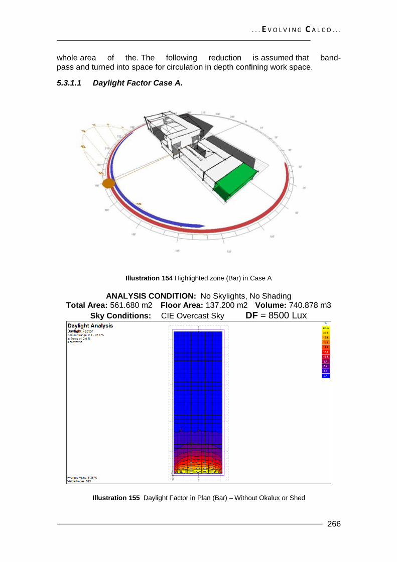
5.3.1.1 Daylight Factor Case A.

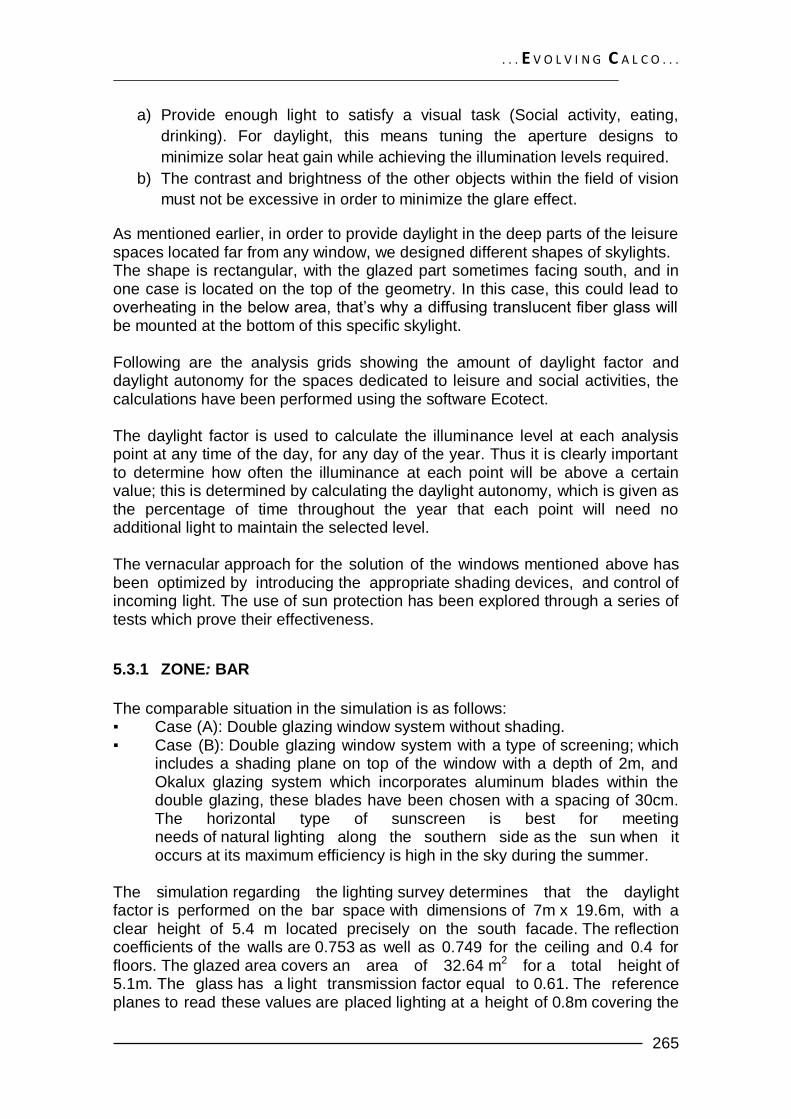
Illustration 154 Highlighted zone (Bar) in Case A

ANALYSIS CONDITION: No Skylights, No Shading

Total Area: 561.680 m2 Floor Area: 137.200 m2 Volume: 740.878 m3

Sky Conditions: CIE Overcast Sky DF = 8500 Lux

Illustration 155 Daylight Factor in Plan (Bar) – Without Okalux or Shed

. . . E V O L V I N G C A L C O . . .

267

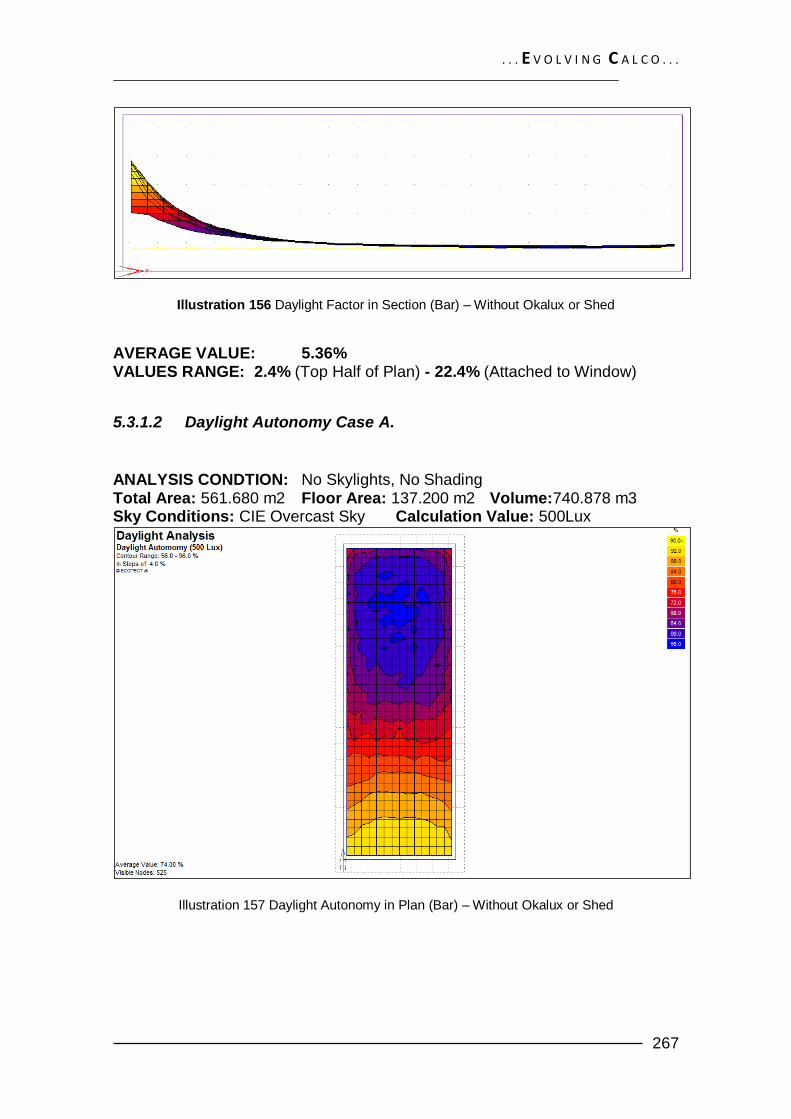
Illustration 156 Daylight Factor in Section (Bar) – Without Okalux or Shed

AVERAGE VALUE: 5.36% VALUES RANGE: 2.4% (Top Half of Plan) - 22.4% (Attached to Window)

5.3.1.2 Daylight Autonomy Case A.

ANALYSIS CONDTION: No Skylights, No Shading Total Area: 561.680 m2 Floor Area: 137.200 m2 Volume:740.878 m3 Sky Conditions: CIE Overcast Sky Calculation Value: 500Lux

Illustration 157 Daylight Autonomy in Plan (Bar) – Without Okalux or Shed

. . . E V O L V I N G C A L C O . . .

268

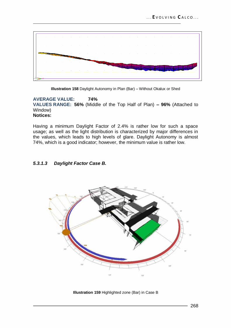
Illustration 158 Daylight Autonomy in Plan (Bar) – Without Okalux or Shed

AVERAGE VALUE: 74% VALUES RANGE: 56% (Middle of the Top Half of Plan) – 96% (Attached to

Window) Notices: Having a minimum Daylight Factor of 2.4% is rather low for such a space usage; as well as the light distribution is characterized by major differences in the values, which leads to high levels of glare. Daylight Autonomy is almost 74%, which is a good indicator; however, the minimum value is rather low.

5.3.1.3 Daylight Factor Case B.

Illustration 159 Highlighted zone (Bar) in Case B

. . . E V O L V I N G C A L C O . . .

269

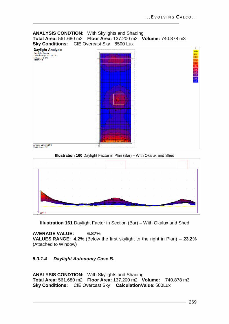
ANALYSIS CONDTION: With Skylights and Shading Total Area: 561.680 m2 Floor Area: 137.200 m2 Volume: 740.878 m3 Sky Conditions: CIE Overcast Sky 8500 Lux

Illustration 160 Daylight Factor in Plan (Bar) – With Okalux and Shed

Illustration 161 Daylight Factor in Section (Bar) – With Okalux and Shed

AVERAGE VALUE: 6.87% VALUES RANGE: 4.2% (Below the first skylight to the right in Plan) – 23.2% (Attached to Window)

5.3.1.4 Daylight Autonomy Case B. ANALYSIS CONDTION: With Skylights and Shading Total Area: 561.680 m2 Floor Area: 137.200 m2 Volume: 740.878 m3 Sky Conditions: CIE Overcast Sky CalculationValue: 500Lux

. . . E V O L V I N G C A L C O . . .

270

Illustration 162 Daylight Autonomy in Plan (Bar) – With Okalux and Shed

Illustration 163 Daylight Autonomy in Section (Bar) – With Okalux and Shed

AVERAGE VALUE: 86.65% VALUES RANGE: 72% (Below the first skylight to the left in Plan) – 92%

(Attached to Window)

Notices:

The minimum value is higher than that of the alternative without Shed or Okalux system. 4.2% is regarded as the minimum for a good visibility in the space with this specific use. Other than that fact, the lighting levels distribution is obviously more coherent. Daylight Autonomy has a higher value as well (87%), which is a good indicator.

. . . E V O L V I N G C A L C O . . .

271

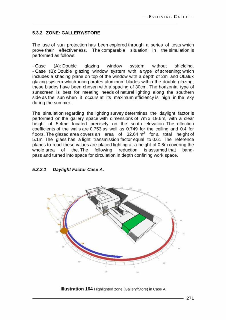
5.3.2 ZONE: GALLERY/STORE

The use of sun protection has been explored through a series of tests which prove their effectiveness. The comparable situation in the simulation is performed as follows: - Case (A): Double glazing window system without shielding. - Case (B): Double glazing window system with a type of screening; which includes a shading plane on top of the window with a depth of 2m, and Okalux glazing system which incorporates aluminum blades within the double glazing, these blades have been chosen with a spacing of 30cm. The horizontal type of sunscreen is best for meeting needs of natural lighting along the southern side as the sun when it occurs at its maximum efficiency is high in the sky during the summer. The simulation regarding the lighting survey determines the daylight factor is performed on the gallery space with dimensions of 7m x 19.6m, with a clear height of 5.4me located precisely on the south elevation. The reflection coefficients of the walls are 0.753 as well as 0.749 for the ceiling and 0.4 for floors. The glazed area covers an area of 32.64 m2 for a total height of 5.1m. The glass has a light transmission factor equal to 0.61. The reference planes to read these values are placed lighting at a height of 0.8m covering the whole area of the. The following reduction is assumed that band-pass and turned into space for circulation in depth confining work space.


Illustration 164 Highlighted zone (Gallery/Store) in Case A

. . . E V O L V I N G C A L C O . . .

272

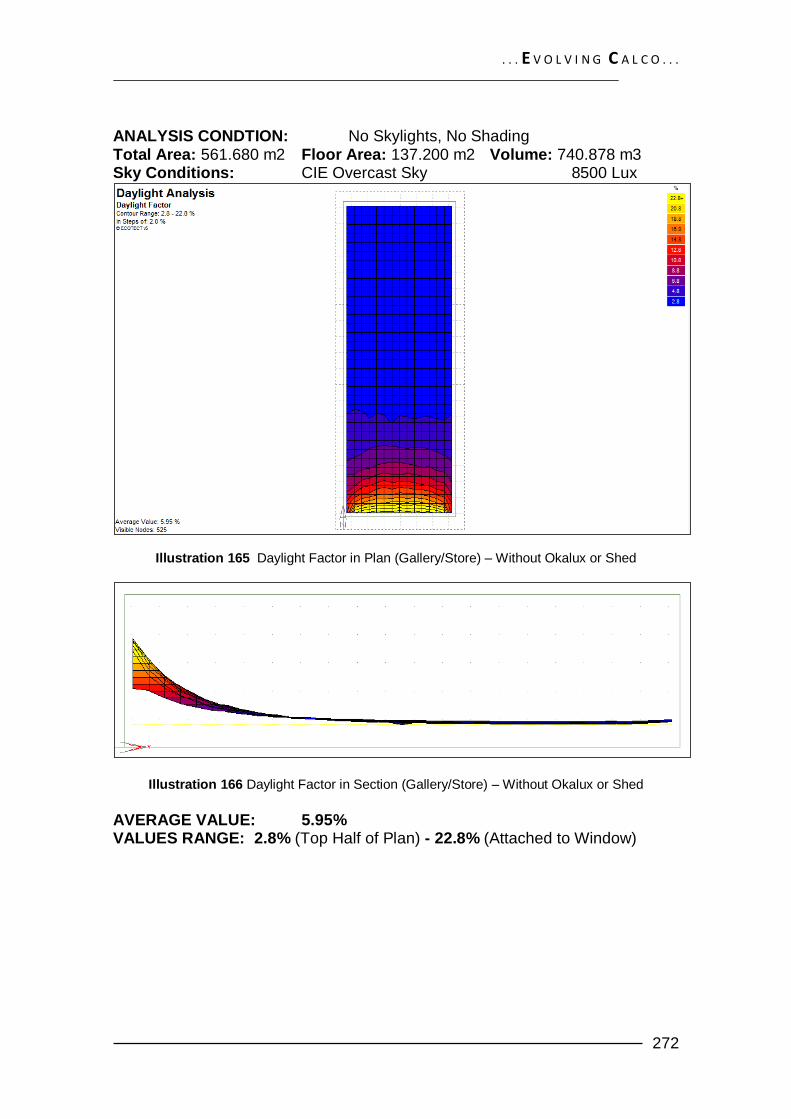
ANALYSIS CONDTION: No Skylights, No Shading Total Area: 561.680 m2 Floor Area: 137.200 m2 Volume: 740.878 m3 Sky Conditions: CIE Overcast Sky 8500 Lux

Illustration 165 Daylight Factor in Plan (Gallery/Store) – Without Okalux or Shed

Illustration 166 Daylight Factor in Section (Gallery/Store) – Without Okalux or Shed

AVERAGE VALUE: 5.95% VALUES RANGE: 2.8% (Top Half of Plan) - 22.8% (Attached to Window)

. . . E V O L V I N G C A L C O . . .

273

5.3.2.2 Daylight Autonomy Case A.

ANALYSIS CONDTION: No Skylights, No Shading Total Area: 561.680 m2 Floor Area: 137.200 m2 Volume: 740.878 m3 Sky Conditions: CIE Overcast Sky 8500 Lux Calculation Value: 500Lux

Illustration 167 Daylight Autonomy in Plan (Gallery/Store) – Without Okalux or

Shed

Illustration 168 Daylight Autonomy in Plan (Gallery/Store) – Without Okalux or Shed

AVERAGE VALUE: 79.41% VALUES RANGE: 63% (Middle of the Top Half) – 103% (Attached to Window)

Notices: Having a minimum Daylight Factor of 2.8% is rather low for such a

space usage; as well as the light distribution is characterized by major differences in the values, which leads to high levels of glare. Daylight Autonomy

. . . E V O L V I N G C A L C O . . .

274

is almost 80%, which is a good indicator; however, the minimum value is rather low.

5.3.2.3 Daylight Factor Case B.

Illustration 169 Highlighted zone (Gallery/Store) in Case B


Illustration 170 Daylight Factor in Plan (Gallery/Store) – With Okalux and Shed

. . . E V O L V I N G C A L C O . . .

275

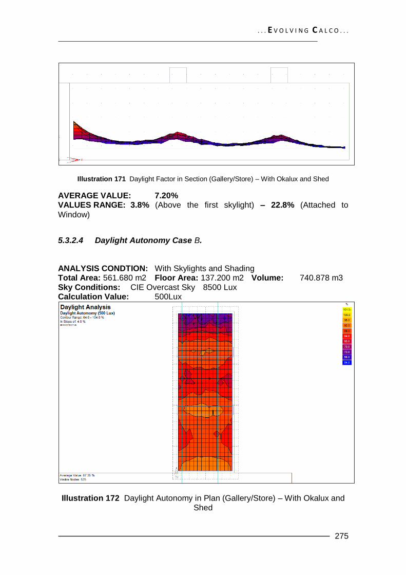
Illustration 171 Daylight Factor in Section (Gallery/Store) – With Okalux and Shed

AVERAGE VALUE: 7.20% VALUES RANGE: 3.8% (Above the first skylight) – 22.8% (Attached to

Window)

5.3.2.4 Daylight Autonomy Case B. ANALYSIS CONDTION: With Skylights and Shading Total Area: 561.680 m2 Floor Area: 137.200 m2 Volume: 740.878 m3 Sky Conditions: CIE Overcast Sky 8500 Lux Calculation Value: 500Lux

Illustration 172 Daylight Autonomy in Plan (Gallery/Store) – With Okalux and Shed

. . . E V O L V I N G C A L C O . . .

276

Illustration 173 Daylight Autonomy in Section (Gallery/Store) – With Okalux and Shed

AVERAGE VALUE: 87.35% VALUES RANGE: 64% (Top of the first skylight) – 97% (Attached to Window)

Notices:

The minimum value is higher than that of the alternative with Shed or Okalux system, 3.8% is regarded a bit less than the minimum for a good visibility in this space, however, the average value is quite good. the increase in lighting due to the skylights contributes much in saving energy within the space. Other than that fact, the lighting levels distribution is obviously more coherent. Daylight Autonomy is 87%, which is a good indicator.

5.3.3 ZONE: Restaurant

The use of sun protection has been explored through a series of tests which prove their effectiveness. The comparable situation in the simulations is as follows: - Case (A): Double glazing window system without shielding. - Case (B): Double glazing window system with a type of screening; which includes a shading plane on top of the window with a depth of 2m, and Okalux glazing system which incorporates aluminum blades within the double glazing, these blades have been chosen with a spacing of 30cm. however, on the western façade, a normal glazing system has been used, since it already incorporates a big shading that covers the whole area (see incident radiation in the next division). The horizontal type of sunscreen is best for meeting needs of natural lighting along the southern side as the sun when it occurs at its maximum efficiency is high in the sky during the summer. The simulation regarding the lighting survey determines the daylight factor are performed on the restaurant space with a floor area of 245.700 m2, with a clear height of 5.4me located precisely on the south and west elevation. The reflection coefficients of the walls are 0.753 as well as 0.749 for the ceiling and 0.4 for floors. The glazed area covers an area of 104.04 m2 for a

. . . E V O L V I N G C A L C O . . .

277

total height of 5.1m. The glass has a light transmission factor equal to 0.61. The reference planes to read these values are placed lighting at a height of 0.8m covering the whole area of the. The following reduction is assumed that band-pass and turned into space for circulation in depth confining work space.


Illustration 174 Highlighted zone (Restaurant) in Case A

Illustration 175 Highlighted zone (Restaurant) in Case B

. . . E V O L V I N G C A L C O . . .

278

ANALYSIS CONDTION: No Skylights, No Shading Total Area: 712.369 m2 Floor Area: 245.700 m2 Volume: 1256.346 m3 Sky Conditions: CIE Overcast Sky 8500 Lux

Illustration 176 Daylight Factor in Plan (Restaurant) – Without Okalux or Shed

Illustration 177 Daylight Factor in Section (Restaurant) – Without Okalux or Shed

AVERAGE VALUE: 13.34% VALUES RANGE: 4.8% (Top Right part of Plan) - 44.8% (Attached to Windows)

. . . E V O L V I N G C A L C O . . .

279

5.3.3.2 Daylight Autonomy Case A. ANALYSIS CONDTION: No Skylights, No Shading Total Area: 712.369 m2 Floor Area: 245.700 m2 Volume: 1256.346 m3 Sky Conditions: CIE Overcast Sky 8500 Lux Calculation Value: 500Lux

Illustration 178 Daylight Autonomy in Plan (Restaurant) – Without Okalux or Shed

Illustration 179 Daylight Autonomy in Plan (Restaurant) – Without Okalux or

Shed

AVERAGE VALUE: 90.45% VALUES RANGE: 81% (Top Right part of Plan) – 97% (Attached to Window)

. . . E V O L V I N G C A L C O . . .

280

Notices: Having a minimum Daylight Factor of 4.8% is quite good for such a

space usage; as for the light distribution, it is characterized by major differences in the values, which leads to high levels of glare. Daylight Autonomy is almost 90%, which is a good indicator.

5.3.3.3 Daylight Factor Case B. ANALYSIS CONDTION: With Skylights and Shading Total Area: 712.369 m2 Floor Area: 245.700 m2 Volume: 1256.346 m3 Sky Conditions: CIE Overcast Sky 8500 Lux

Illustration 180 Daylight Factor in Plan (Restaurant) – With Okalux and Shed

Illustration 181 Daylight Factor in Section (Restaurant) – With Okalux and Shed

. . . E V O L V I N G C A L C O . . .

281

AVERAGE VALUE: 10.45% VALUES RANGE: 4% (Top Right part of Plan) – 24% (Attached to Windows)

5.3.3.4 Daylight Autonomy Case B.

ANALYSIS CONDTION: With Skylights and Shading Total Area: 712.369 m2 Floor Area: 245.700 m2 Volume:

1256.346 m3 Sky Conditions: CIE Overcast Sky 8500 Lux Calculation Calculation Value: 500Lux

Illustration 182 Daylight Autonomy in Plan (Restaurant) – With Okalux and Shed

Illustration 183 Daylight Autonomy in Section (Restaurant) – With Okalux and Shed

. . . E V O L V I N G C A L C O . . .

282

AVERAGE VALUE: 88.64% VALUES RANGE: 78% (Top Right part of Plan) – 97% (Attached to Windows)

Notices:

The minimum is higher than that of this alternative 4% is regarded the minimum for a good visibility in this space, however, the average DF value is quite good. The lighting levels distribution is obviously more coherent. Daylight Autonomy is 89%, which is a good indicator.

5.3.4 ZONE: TRANSITIONAL ZONE

The values used in the test are extracted from the manufacturers’ information. The situation in the simulations is as follows: - Case (A): 3-layer ETFE cushions. The system allows for a change in the shading due to the air pressure. This can be useful to acquire more shade in the summer to reduce the heat gains, and vice versa in the winter. The ETFE system include panels with dimensions of 3mx25m, 3mx9m, and 3mx6m… the fixed 3m width of the panels is intentionally the same in order to have an effective depth to thermal behavior ratio. The simulation regarding the lighting survey determines the daylight factor are performed on the transitional zone with a floor area of 61.346 m2, with a clear height of 9m from zero level, and 14m from basement, located precisely on the south and west elevation. The reflection coefficients of the walls are 0.753 as well as 0.749 for the ceiling and 0.4 for floors. The glazed area covers an area of 891.945 m2 for a total height of 8.7m from zero level. The glass has a light transmission factor equal to 0.8. The reference planes to read these values are placed lighting at a height of 0.8m covering the whole area of the. The following reduction is assumed that band-pass and turned into space for circulation in depth confining work space.

. . . E V O L V I N G C A L C O . . .

283

5.3.4.1 Daylight Factor Case A

Illustration 184 Highlighted zone (Transitional zone) in Case A


Illustration 185 Daylight Factor in Plan (T.Z.(A)) – With ETFE

. . . E V O L V I N G C A L C O . . .

284

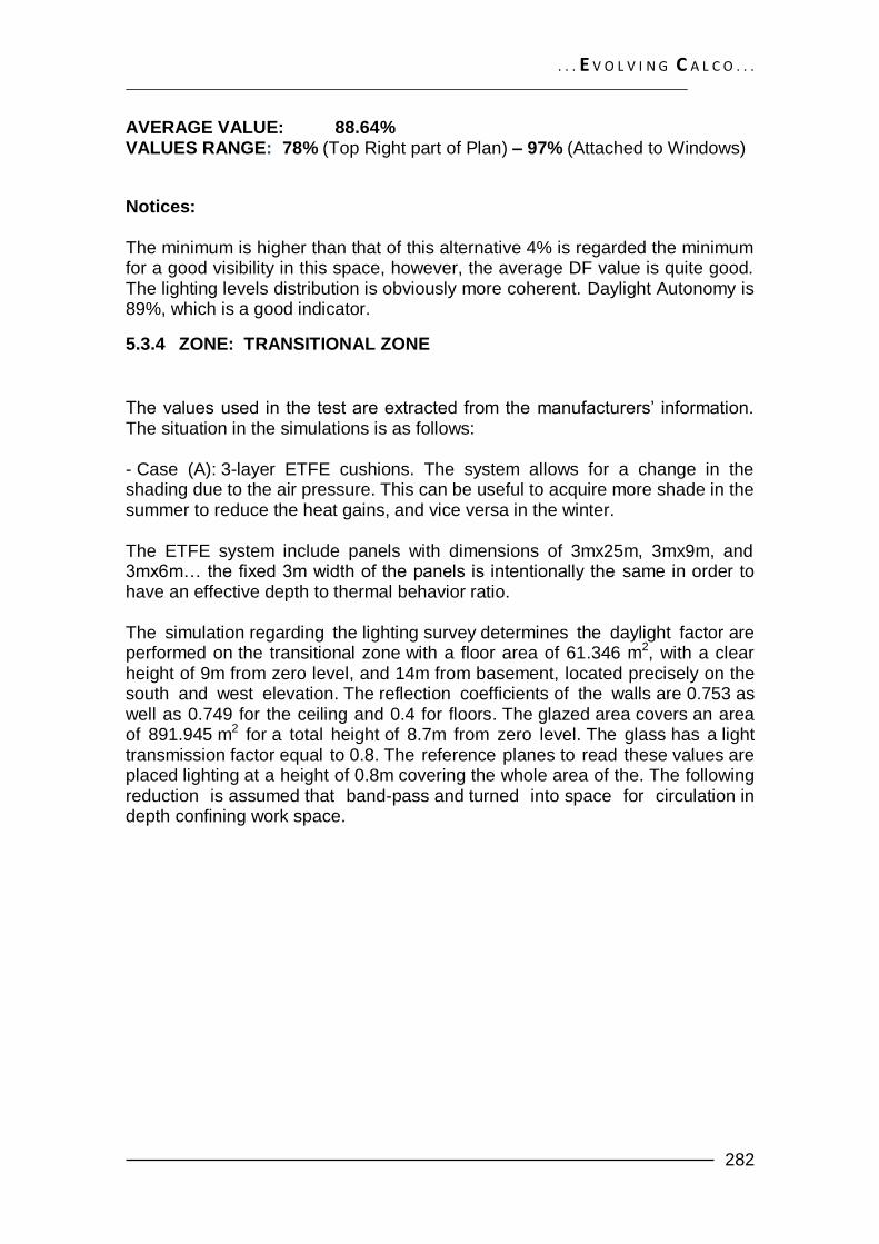
Illustration 186 Daylight Factor in Section (T.Z.(A)) – With ETFE

AVERAGE VALUE: 48.35% VALUES RANGE: 6.9% (Top of Plan) – 67% (Attached to Windows)

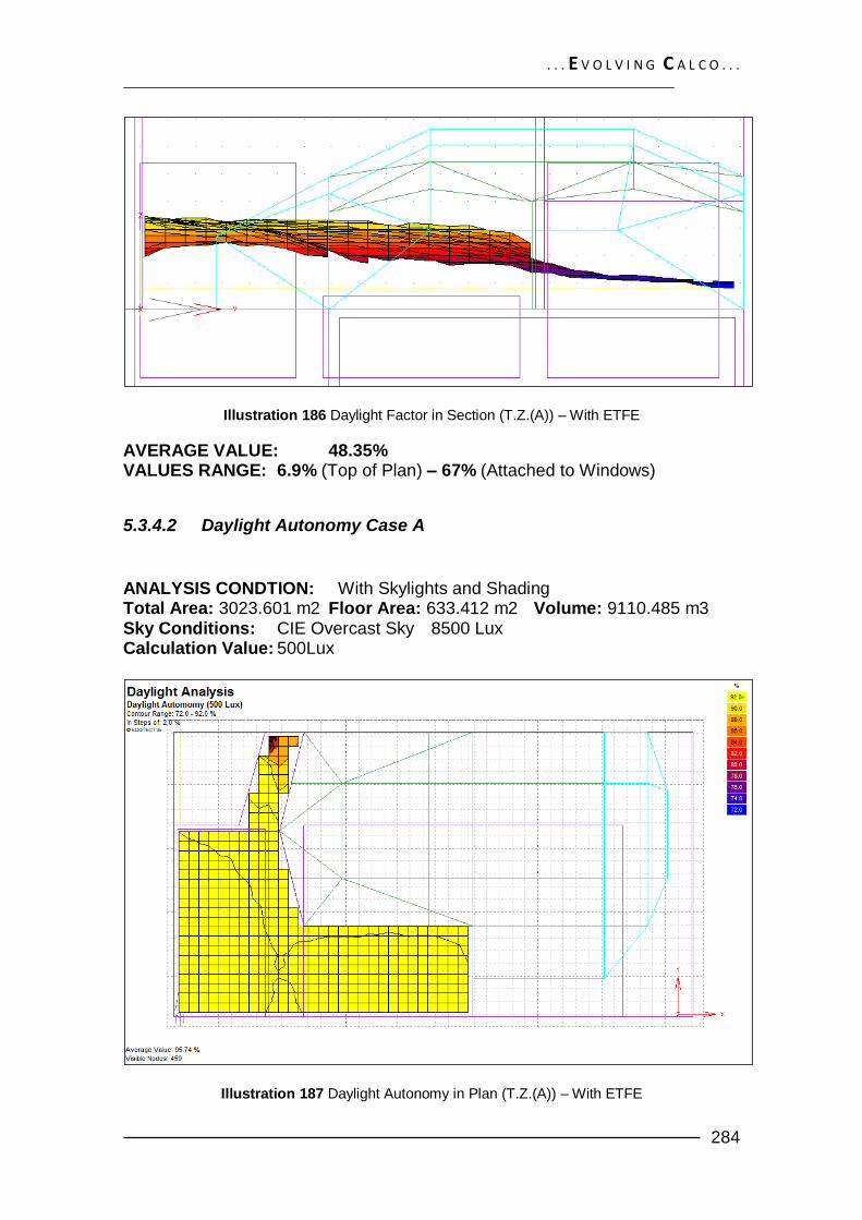
5.3.4.2 Daylight Autonomy Case A

ANALYSIS CONDTION: With Skylights and Shading Total Area: 3023.601 m2 Floor Area: 633.412 m2 Volume: 9110.485 m3 Sky Conditions: CIE Overcast Sky 8500 Lux Calculation Value: 500Lux

Illustration 187 Daylight Autonomy in Plan (T.Z.(A)) – With ETFE

. . . E V O L V I N G C A L C O . . .

285

Illustration 188 Daylight Autonomy in Section (T.Z.(A)) – With ETFE

AVERAGE VALUE: 95.74% VALUES RANGE: 72% (Top of Plan) – 92% (Attached to Windows) Notices: In this space, on the zero level, with a clear height of 9m; daylight factor minimum value is 6.9% which is good. The average DF value is very good for such a space usage, on the bright days; the ETFE air pressure mechanism can change the shading value to reach better results.

5.3.4.3 Daylight Factor Case B

Illustration 189 Highlighted zone (Transitional zone) in Case B

. . . E V O L V I N G C A L C O . . .

286


Illustration 190 Daylight Factor in Plan (T.Z.(B)) – With ETFE

Illustration 191 Daylight Factor in Section (T.Z.(B)) – With ETFE

AVERAGE VALUE: 15.01% VALUES RANGE: 7% (Under the stairs) – 25% (Close to Windows)

. . . E V O L V I N G C A L C O . . .

287

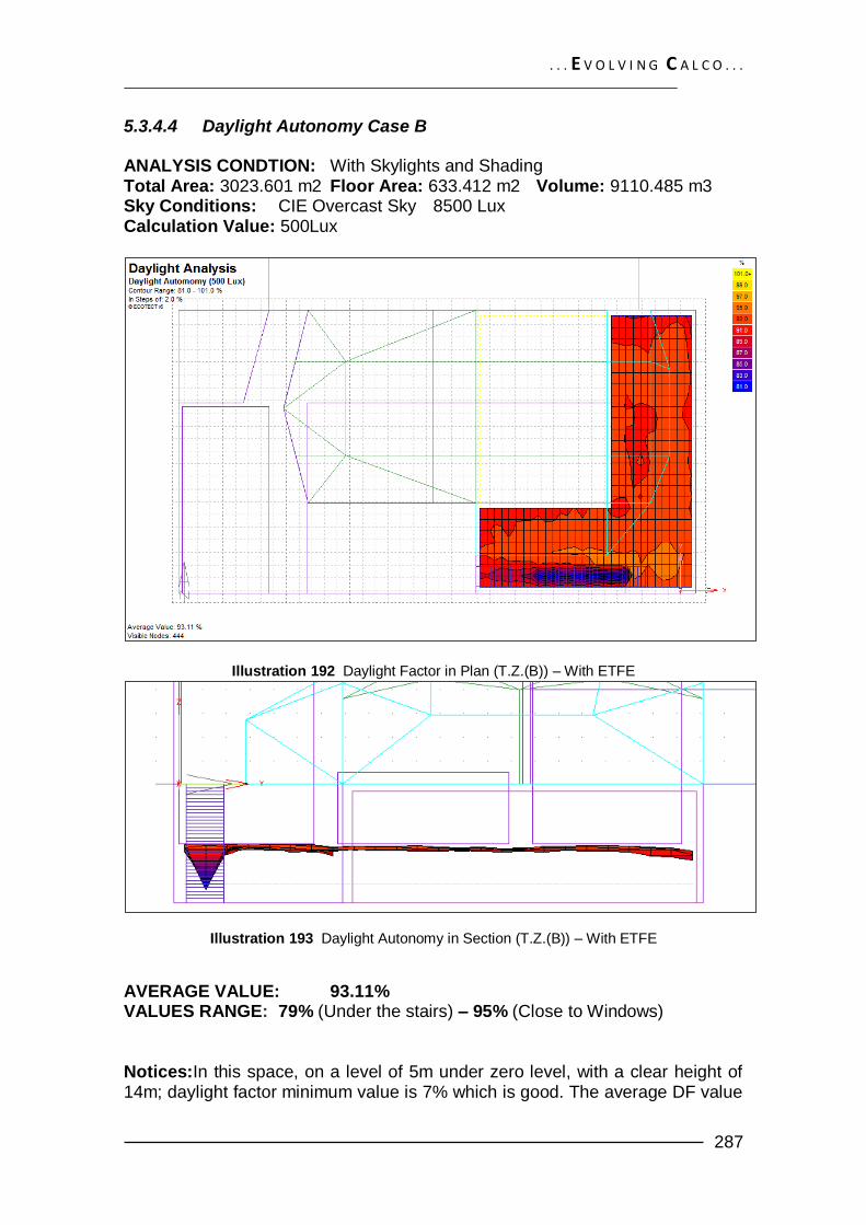
5.3.4.4 Daylight Autonomy Case B ANALYSIS CONDTION: With Skylights and Shading Total Area: 3023.601 m2 Floor Area: 633.412 m2 Volume: 9110.485 m3 Sky Conditions: CIE Overcast Sky 8500 Lux Calculation Value: 500Lux

Illustration 192 Daylight Factor in Plan (T.Z.(B)) – With ETFE

Illustration 193 Daylight Autonomy in Section (T.Z.(B)) – With ETFE

AVERAGE VALUE: 93.11% VALUES RANGE: 79% (Under the stairs) – 95% (Close to Windows) Notices:In this space, on a level of 5m under zero level, with a clear height of 14m; daylight factor minimum value is 7% which is good. The average DF value

. . . E V O L V I N G C A L C O . . .

288

is acceptable. The lighting levels distribution is coherent. Daylight Autonomy is 93%, which is a very good indicator.

5.3.5 ZONE: EXHIBITION HALL

5.3.5.1 Daylight Factor Case A ANALYSIS CONDTION: With Skylights and Shading Total Area: 692.220 m2 Floor Area: 207.810 m2 Volume: 1039.043 m3 Sky Conditions: CIE Overcast Sky 8500 Lux

Illustration 194 Daylight Factor in Plan (Exhibition)

Illustration 195 Daylight Factor in Section (Exhibition)

AVERAGE VALUE: 6.07% VALUES RANGE: 3.8% (Upper left part of Plan) – 20.63% (Close to Windows)

. . . E V O L V I N G C A L C O . . .

289

5.3.5.2 Daylight Autonomy Case A ANALYSIS CONDTION: With Skylights and Shading Total Area: 692.220 m2 Floor Area: 207.810 m2 Volume: 1039.043 m3 Sky Conditions: CIE Overcast Sky 8500 Lux Calculation Value: 500Lux

Illustration 196 Daylight Factor in Plan (Exhibition)

Illustration 197 Daylight Autonomy in Section (Exhibition)

AVERAGE VALUE: 83.12% VALUES RANGE: 72% (Upper left part of Plan) – 92% (Close to Windows)

Notices:

In this space, on a level of 5m under zero level, with a clear height of 4m; it’s clear that in order to have a clear vision, an adequate amount of artificial lighting needs to be installed, not only for the fact that the minimum daylight factor value

. . . E V O L V I N G C A L C O . . .

290

is 3.8% (which is lower than the minimum preferable value, but also due to the function. The average DF value is acceptable. The lighting levels distribution is coherent. Daylight Autonomy is 83%, which is a good indicator. CONCLUSION

As we can see from these graphs, the interior of the inner parts of the bar and gallery is trend to present high opacity and although it has a minimum of 4% which is considered sufficient as a minimum value for such an use, outside of a one which requires lighting for activities that involve concentration, such as in a school. The restaurant on the other hand presents fairly homogeneous lighting values, a factor which increases the sense of comfort within the space. The Theater use determines the fact that natural lighting will not be of importance. The rectangular lines visible in the graphs represent the roof skylights above the bar, gallery and restaurent, which increase the lighting levels within the spaces, their contribution is specifically important in the deep parts of these spaces. As for the layout of the furniture, obviously it will affect the distribution of light in different areas, important to avoid creating shade; it was decided to use the model Okalux RETRO which is an insulating glass which contains specially shaped reflective blades in the cavity perpendicular to the direction of the glazed surface; that allows sunlight to guarantee better illumination and penetration of the light to the interior of the building.

. . . E V O L V I N G C A L C O . . .

291

5.4 SOLAR EXPOSURE ANALYSIS (Incident Solar Radiation) Incident solar radiation, also termed ―insolation‖, refers to the wide spectrum radiant energy from the Sun which strikes an object or surface within the building. This includes both a direct component from the Sun itself (sunshine) and a diffuse component from the visible sky (skylight).

The direct component (Edirect) is given as a value in W/m² and is measured on a

surface directly facing the Sun. As the Sun moves through the sky, this measurement surface tracks it so that the direction of incident radiation is always normal (straight on) to it.

The diffuse component (Ediffuse) is also given in W/m² and is taken as the

energy available from the entire sky dome, minus the direct radiation value, as measured on a flat horizontal surface. Once this value is known, it can be moderated by the tilt angle of each surface in the model. For example a vertical surface, no matter which way it faces, will only ever see at best one half of the sky dome - meaning that will only ever receive half of the available diffuse component. A horizontal surface that faces upwards, however, it will see it all. It is important to note that ―insolation‖ refers only to the amount of energy actually falling on a surface, which is not affected in any way by the surface properties of materials or by any internal refractive effects. Material properties only affect the amount of solar radiation absorbed and/or transmitted by a surface, which are idle in this case.

Insolation (Eincident) is therefore affected only by the angle of incidence of the

radiation (A), the fraction of the surface currently in shadow from other

surrounding geometry (Fshad), the fraction of the diffuse sky actually visible from

the surface (Fsky) and, if a surface is partially adjacent to another zone, the area

of surface actually exposed to solar radiation (ExposedArea). These factors

affect the beam normal (Ebeam) and diffuse sky (Ediffuse) radiation differently,

such that:

Eincident = [(Ebeam x cos(A) x Fshad) + (Ediffuse x Fsky)] x ExposedArea

. . . E V O L V I N G C A L C O . . .

292

5.4.1 South Elevation

Illustration 198 Total Monthly Solar Exposure – SOUTH ELEV – Without Okalux or Shed

Illustration 199 Total Monthly Solar Exposure – SOUTH ELEV – With Okalux

. . . E V O L V I N G C A L C O . . .

293

Table 25 Shading Contribution Due to Okalux

Illustration 200 Total Monthly Solar Exposure – SOUTH ELEV – With Okalux+Shed

. . . E V O L V I N G C A L C O . . .

294

Table 26 Shading Contribution Due to Okalux+SHED

5.4.2 West Elevation

Illustration 201 Total Monthly Solar Exposure – WEST ELEV – Without Shed

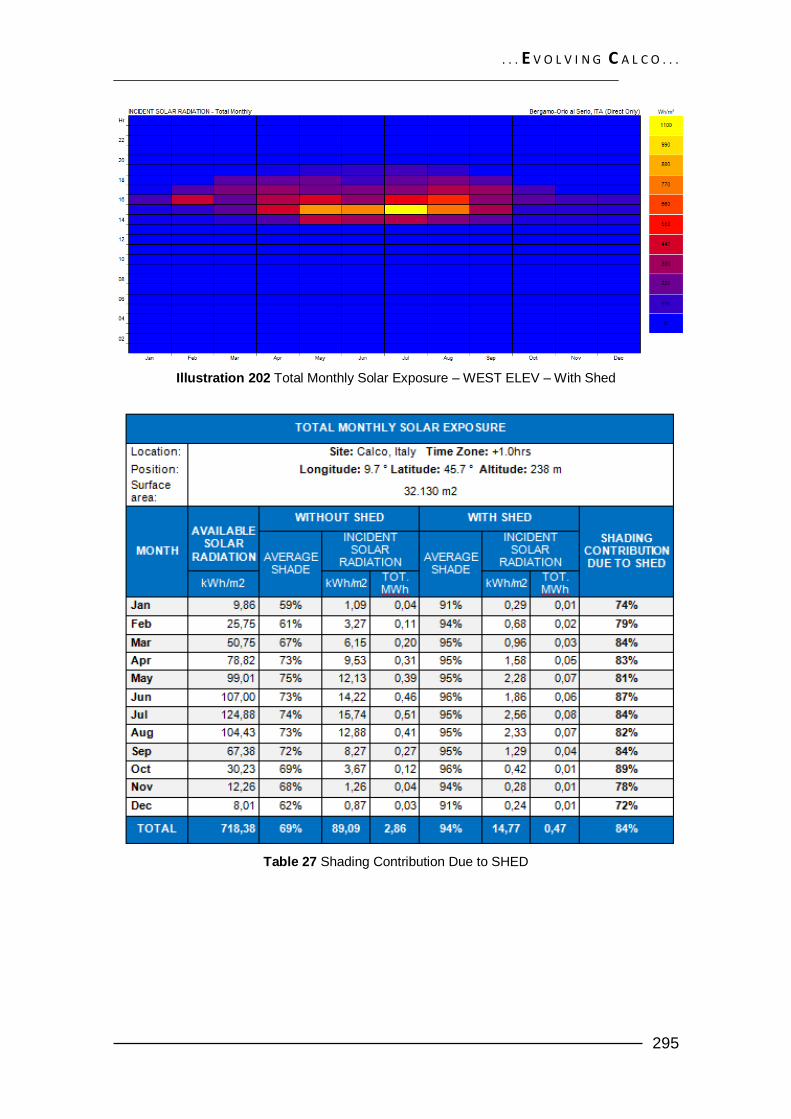
. . . E V O L V I N G C A L C O . . .

295

Illustration 202 Total Monthly Solar Exposure – WEST ELEV – With Shed

Table 27 Shading Contribution Due to SHED

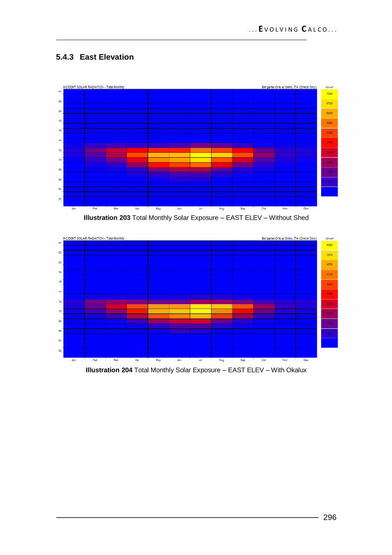
. . . E V O L V I N G C A L C O . . .

296

5.4.3 East Elevation

Illustration 203 Total Monthly Solar Exposure – EAST ELEV – Without Shed

Illustration 204 Total Monthly Solar Exposure – EAST ELEV – With Okalux

. . . E V O L V I N G C A L C O . . .

297

Table 28 Shading Contribution Due to OKALUX

Illustration 205 Total Monthly Solar Exposure – EAST ELEV – With Okalux + Shed

. . . E V O L V I N G C A L C O . . .

298

Table 29 Shading Contribution Due to OKALUX+SHED

CONCLUSION

This section determines the period over which solar radiation values will be calculated monthly, and how the results will be displayed in each graph. All such calculations are based on the hourly beam normal and diffuse horizontal solar radiation values in the currently loaded climate data set.

. . . E V O L V I N G C A L C O . . .

299

6 THERMAL ANALYSIS

6.1 INTRODUCTION:

Buildings are usually designed to provide shelter as well as thermal comfort in the occupied space, backed up by mechanical heating and air-conditioning systems as necessary. The envelope of the building is a transition space through which interaction between indoor and outdoor environment takes place. The selection and arrangement of building envelope components can significantly impact its thermal performance which is a determining factor in its consumption of energy. In dealing with the building as a thermal system, the proper selection of its components and their relationships is of great importance in order to optimize its performance. The aim of this chapter of the thesis is to describe the basic building thermal design optimization model of the proposed project by defining building design variables, a criterion of optimality, constraints, and a suitable thermal simulation model integrated into the optimization technique. This leads to the general aim of the thesis, which is to design a thermally optimum building with minimum reliance upon mechanical systems, in order not to sacrifice neither aesthetics nor function of the building. Building design is a decision making process in which decisions are made on the shape, orientation and selection of the physical components of the building and their arrangements to achieve certain objectives. These decisions are usually limited by certain constraints some of which are outside the control of the designer. The framework of input, process and output approach is influenced by many factors in the building design process: 121 Inputs:

Design know-how (professional and Technical:

Climatic conditions Energysources

Objectives:

Human needs Social needs Environmental objectives Technical objectives

Constraints: Cost Technology Human characteristics

121

DEGELMAN, Legel et allTthe framework of an optimization model for the thermal design of building envelopes.

Proceedings of the Ninth Symposium on Improving Building Systems in Hot and Humid Climate. Argton texas.1994 p

105

. . . E V O L V I N G C A L C O . . .

300

Physical environment Aesthetics Practicality

6.2 OBJECTIVE FUNCTION

The ultimate goal of building design is to provide occupants with a comfortable environment. In order to determine an optimum thermal design performance based on occupant comfort, it is necessary to establish a relationship between thermal comfort and the factors that have an impact on the thermal performance of buildings. The relationship can then be used to select an optimum combination of building design parameters that achieve the desired objectives. In order to control the design process in a systematic approach, it is necessary to formulate a criterion that can be used to compare the process outputs to objectives. Building thermal design can be optimized with the objective of minimizing building capital and operating cost, minimizing thermal load or minimizing thermal discomfort in the occupied space.

6.3 BUILDING THERMAL PERFORMANCE SIMULATION:

Ecotect was found to adequately represent the specified building thermal design parameters with accuracy while maintaining simplicity of simulation. The simulation program will be used to evaluate the annual heating/cooling loads depending on which type of system used to provide them, in this case, a Mixed Mode Ventilation system is used. This system has been chosen in the analysis, since it’s similar to that of the one used in the research. It is a combination of air-conditioning and natural ventilation where the HVAC system shuts down whenever outside conditions are within the defined thermostat range. It should be noted that Ecotect assumes that either the system continues running on an supplying mechanical ventilation or the windows are opened. In either case, the air change rate increases as described above. Note also that Ecotect does not consider energy used in the ducting of air when it calculates heating and cooling loads - these are both given as space loads not plant loads. The analysis will be made considering two cases:

- Case A: in which the wall layers and U-Values are the ones designed by the researchers in Chapter 5

- Case B: in which a standard walls, roofs and slabs systems have been assigned to the building. The chosen systems are described in details in table 30

This comparison will show the difference in performance tested results for air-conditioned buildings between the two cases, as will be shown later on. This difference will determine the enhancement or degradation in the building thermal performance.

. . . E V O L V I N G C A L C O . . .

301

6.3.1 Considerations for the demand of the various zones:

6.3.1.1 Skin layers and U-values CASE A:

Details are explained in Chapter 5 CASE B:

SKIN TYPE LAYERS U-VALUE

Outer Walls

(Brick Timber Frame) 110mm external brick plus, 75mm timber frame with 10mm plasterboard inside.

1.77

W/m2.K

Inner Partitions

(Framed Plasterboard) 80mm framed wall as air gap, with 10mm plaster board either side.

2.2 W/m2.K

Roof Slab

(Concrete Roof Asphalt)

6mm asphalt cover, with 150mm concrete lightweight, and 10mm Plaster Building (Molded Dry).

0.896

W/m2.K

Floor Slab

(Concrete Slab On Ground)

100mm thick concrete slab on ground, with 1500mm Soil layer (Avg. Properties)

0.88 W/m2.K

Table 30 Input data for calculation case B

6.3.1.2 System occupancy (for both cases A and B) BAR The number of users of the bar expecting 1.5 rotations in average per day during the day = 1.5 * 40 = 60 people. AUDITORIUM The number of users for the Auditorium/Hall will be equal to its maximum capacity (300 people). GALLERY (STORE)

Te number of sellers is considered to be 2 for the gallery/store. RESTAURANT: The number of users for the restaurant/bar is considered to take into account 1.5 average rotations in the capacity of the tables per day = 1.5 * 70 = 105 people All the facilities (except the Auditorium/hall) will be considered to run for a total period of labor = 365 days - 12 celebrations days – 15 days Ferr-August – 5 days Eastern - 50 Sundays = 283 days.

. . . E V O L V I N G C A L C O . . .

302

The Auditorium/hall is considered to be used for an average of 3 times per week without taking into account holidays, in this way, the number of days of usage is = 156 – 6 days Ferr-August – 3 days Eastern = 147 days. For the sake of simplificity it is considered a constant demand of users throughout the year represented as an average of the possible number of users per month.

6.3.2 Heating & Cooling Loads

6.3.2.1 Auditorium / Hall

CASE A

Analyzed Zone: All thermal Zones within the Auditorium / Hall

Active System: Mixed Mode Ventilation. Comfort band/thermostat range: Varies depending on Zone Operation: Varies depending on Zone Occupancy: Varies depending on Zone

Illustration 206 Total monthly Heating/Cooling Loads Auditorium Hall building (CASE A)

MONTHLY HEATING & COOLING LOADS MONTH HEATING (Wh) COOLING (Wh) TOTAL (Wh)

Jan 5,659,496 0 5,659,496 Feb 3,700,882 0 3,700,882 Mar 2,811,215 165,634 2,976,848 Apr 1,309,480 720,398 2,029,878 May 265,568 918,046 1,183,613 Jun 27,842 475,559 503,401

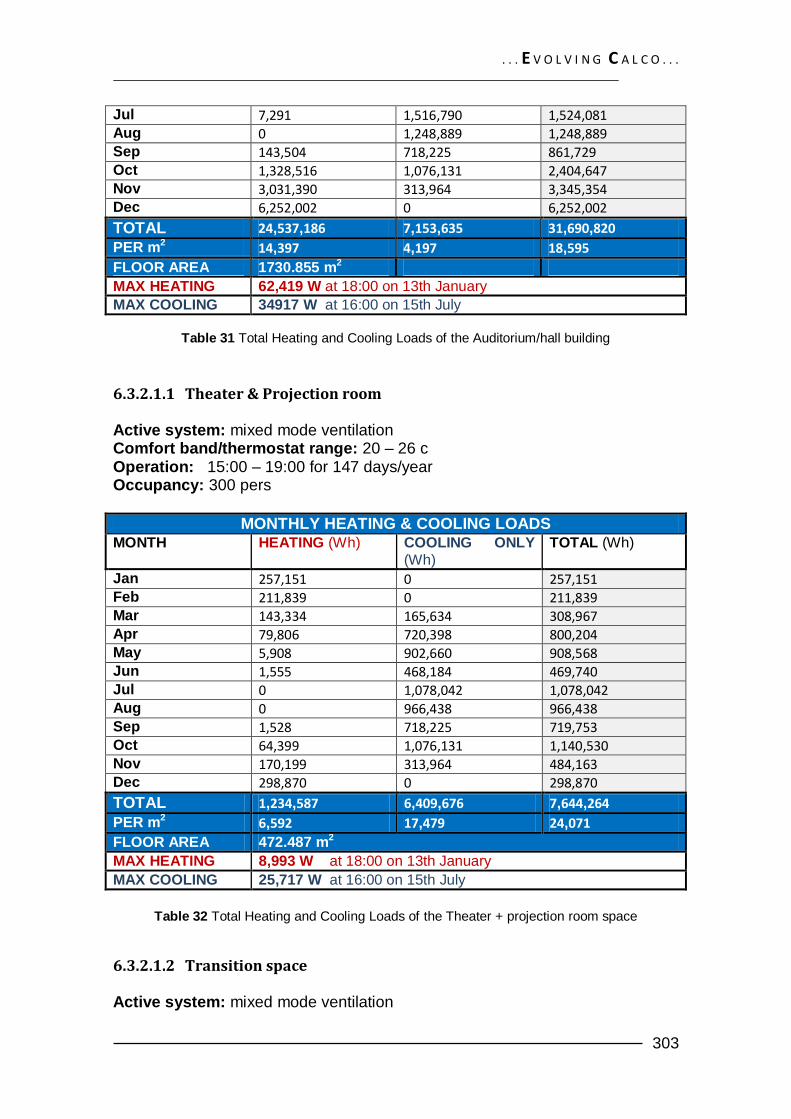
. . . E V O L V I N G C A L C O . . .

303

Jul 7,291 1,516,790 1,524,081 Aug 0 1,248,889 1,248,889 Sep 143,504 718,225 861,729 Oct 1,328,516 1,076,131 2,404,647 Nov 3,031,390 313,964 3,345,354 Dec 6,252,002 0 6,252,002

TOTAL 24,537,186 7,153,635 31,690,820

PER m2 14,397 4,197 18,595

FLOOR AREA 1730.855 m2

MAX HEATING 62,419 W at 18:00 on 13th January

MAX COOLING 34917 W at 16:00 on 15th July

Table 31 Total Heating and Cooling Loads of the Auditorium/hall building

6.3.2.1.1 Theater & Projection room Active system: mixed mode ventilation Comfort band/thermostat range: 20 – 26 c Operation: 15:00 – 19:00 for 147 days/year Occupancy: 300 pers

MONTHLY HEATING & COOLING LOADS MONTH HEATING (Wh) COOLING ONLY

(Wh)

TOTAL (Wh)

Jan 257,151 0 257,151 Feb 211,839 0 211,839 Mar 143,334 165,634 308,967 Apr 79,806 720,398 800,204 May 5,908 902,660 908,568 Jun 1,555 468,184 469,740 Jul 0 1,078,042 1,078,042 Aug 0 966,438 966,438 Sep 1,528 718,225 719,753 Oct 64,399 1,076,131 1,140,530 Nov 170,199 313,964 484,163 Dec 298,870 0 298,870

TOTAL 1,234,587 6,409,676 7,644,264

PER m2 6,592 17,479 24,071



MAX COOLING 25,717 W at 16:00 on 15th July

Table 32 Total Heating and Cooling Loads of the Theater + projection room space

6.3.2.1.2 Transition space Active system: mixed mode ventilation

. . . E V O L V I N G C A L C O . . .

304

Comfort band/thermostat range: 16 – 31 c Operation: 09:00 – 21:00 for 147 days/year Occupancy: 30 pers


Jan 4,079,970 0 4,079,970 Feb 2,454,666 0 2,454,666 Mar 1,819,071 0 1,819,071 Apr 734,683 0 734,683 May 145,224 0 145,224 Jun 8,720 0 8,720 Jul 7,291 0 7,291 Aug 0 0 0 Sep 89,948 0 89,948 Oct 916,089 0 916,089 Nov 2,032,064 0 2,032,064 Dec 4,537,832 0 4,537,832

TOTAL 16,825,558 0 16,825,558

PER m2 26,563 0 26,563


MAX HEATING 52,073 W at 21:00 on 17th December

MAX COOLING NO COOLING

Table 33 Total Heating and Cooling Loads of the Transition space

6.3.2.1.3 Gallery/exhibition hall Active system: mixed mode ventilation Comfort band/thermostat range: 20 – 26 c Operation: 09:00 – 21:00 for 147 days/year Occupancy: 20 pers


Jan 978,193 0 978,193 Feb 780,504 0 780,504 Mar 662,147 0 662,147 Apr 403,620 0 403,620 May 105,065 12776 117,841 Jun 16,225 7374 23,599 Jul 0 285452 285,452 Aug 0 174520 174,520 Sep 48,095 0 48,095 Oct 284,592 0 284,592 Nov 646,863 0 646,863 Dec 1,034,996 0 1,034,996

. . . E V O L V I N G C A L C O . . .

305

TOTAL 4,960,300 480,122 5,440,422

PER m2 23,869 2,310 26,180


MAX HEATING 6,737 W at 21:00 on 17th December

MAX COOLING 3,664 W at 16:00 on 15th July

Table 34 Total Heating and Cooling Loads of the Gallery/exhibition space

6.3.2.1.4 Services Active system: mixed mode ventilation

Comfort band/thermostat range: 20 – 26 c

Operation: 15:00 – 19:00 for 147 days/year

Occupancy: 30 pers


Jan 344,182 0 344,182 Feb 253,875 0 253,875 Mar 186,664 0 186,664 Apr 91,373 0 91,373 May 9,370 2,609 11,980 Jun 1,342 0 1,342 Jul 0 153,296 153,296 Aug 0 107,932 107,932 Sep 3,932 0 3,932 Oct 63,436 0 63,436 Nov 182,265 0 182,265 Dec 380,304 0 380,304

TOTAL 1,516,744 263,837 1,780,581

PER m2 16,001 2,876 18,878



MAX COOLING 5,491 W at 17:00 on 3rd of August

Table 35 Total Heating and Cooling Loads of the Services spaces

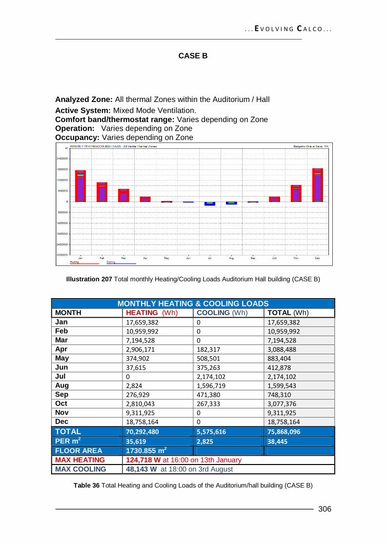
. . . E V O L V I N G C A L C O . . .

306

CASE B

Analyzed Zone: All thermal Zones within the Auditorium / Hall

Active System: Mixed Mode Ventilation. Comfort band/thermostat range: Varies depending on Zone Operation: Varies depending on Zone Occupancy: Varies depending on Zone

Illustration 207 Total monthly Heating/Cooling Loads Auditorium Hall building (CASE B)


Jan 17,659,382 0 17,659,382 Feb 10,959,992 0 10,959,992 Mar 7,194,528 0 7,194,528 Apr 2,906,171 182,317 3,088,488 May 374,902 508,501 883,404 Jun 37,615 375,263 412,878 Jul 0 2,174,102 2,174,102 Aug 2,824 1,596,719 1,599,543 Sep 276,929 471,380 748,310 Oct 2,810,043 267,333 3,077,376 Nov 9,311,925 0 9,311,925 Dec 18,758,164 0 18,758,164

TOTAL 70,292,480 5,575,616 75,868,096

PER m2 35,619 2,825 38,445



MAX COOLING 48,143 W at 18:00 on 3rd August

Table 36 Total Heating and Cooling Loads of the Auditorium/hall building (CASE B)

. . . E V O L V I N G C A L C O . . .

307

6.3.2.2 Restaurant/ bars

CASE A

Analyzed Zone: All thermal Zones within the Restaurant, Bar and Gallery Zone

Active System: Mixed Mode Ventilation. Comfort band/thermostat range: 20 – 26 c Operation: 09:00 – 21:00 for 283 days/year Occupancy: Varies depending on Zone

Illustration 208 Total monthly Heating/Cooling Loads Restaurant/bar building (CASE A)


Jan 3,314,371 0 3,314,371 Feb 2,209,749 0 2,209,749 Mar 1,655,612 0 1,655,612 Apr 862,115 0 862,115 May 184,992 0 184,992 Jun 49,837 0 49,837 Jul 7,342 598,876 606,217 Aug 1,000 537,051 538,051 Sep 125,353 0 125,353 Oct 759,421 0 759,421 Nov 1,950,652 0 1,950,652 Dec 3,417,294 0 3,417,294

TOTAL 14,537,738 1,135,926 15,673,664

PER m2 22,872 1,787 24,660

FLOOR AREA 635,6 m2

MAX HEATING 19,827 W at 21:00 on 17th of December

. . . E V O L V I N G C A L C O . . .

308

MAX COOLING 11,855 W at 13:00 on 2ND of August

Table 37 Total Heating and Cooling Loads of the Restaurant/bar building

6.3.2.2.1 Bar Active system: Natural Ventilation and radiant floor

Comfort band/thermostat range: 20– 26 c


Occupancy: 60 pers


Jan 593,867 0 593,867 Feb 391,676 0 391,676 Mar 285,002 0 285,002 Apr 141,673 0 141,673 May 24,268 0 24,268 Jun 6,122 0 6,122 Jul 776 73,416 74,192 Aug 0 82,509 82,509 Sep 15,691 0 15,691 Oct 122,948 0 122,948 Nov 336,766 0 336,766 Dec 610,110 0 610,110

TOTAL 2,528,898 155,925 2,684,823

PER m2 18,432 1,136 19,569

FLOOR AREA 137.2 m2



Table 38 Total Heating and Cooling Loads of the Bar space

6.3.2.2.2 Gallery/store Active system: Natural ventilation and radiant floor



Occupancy: 20 pers


Jan 566,662 0 566,662 Feb 371,637 0 371,637 Mar 274,289 0 274,289

. . . E V O L V I N G C A L C O . . .

309

Apr 139,337 0 139,337 May 26,665 0 26,665 Jun 6,845 0 6,845 Jul 876 90,947 91,824 Aug 0 91,044 91,044 Sep 16,221 0 16,221 Oct 120,296 0 120,296 Nov 320,607 0 320,607 Dec 582,564 0 582,564

TOTAL 2,426,000 181,991 2,607,992

PER m2 17,682 1,326 19,009

FLOOR AREA 137.2 m2



Table 39 Total Heating and Cooling Loads of the Gallery/store space

6.3.2.2.3 Restaurant Active system: natural ventilation and radiant floor



Occupancy: 105pers


Jan 1,736,677 0 1,736,677 Feb 1,138,797 0 1,138,797 Mar 856,002 0 856,002 Apr 446,015 0 446,015 May 109,712 0 109,712 Jun 31,118 0 31,118 Jul 5,472 403,268 408,740 Aug 1,000 328,631 329,631 Sep 83,014 0 83,014 Oct 425,626 0 425,626 Nov 1,051,534 0 1,051,534 Dec 1,798,819 0 1,798,819

TOTAL 7,683,787 731,899 8,415,686

PER m2 31,273 2,979 34,252

FLOOR AREA 245.7 m2



Table 40 Total Heating and Cooling Loads of the Restaurant space

. . . E V O L V I N G C A L C O . . .

310

6.3.2.2.4 Services Active system: mixed mode ventilation



Occupancy: 10 pers


Jan 417,164 0 417,164 Feb 307,639 0 307,639 Mar 240,319 0 240,319 Apr 135,091 0 135,091 May 24,346 0 24,346 Jun 5,752 0 5,752 Jul 217 31,245 31,462 Aug 0 34,866 34,866 Sep 10,427 0 10,427 Oct 90,552 0 90,552 Nov 241,746 0 241,746 Dec 425,803 0 425,803

TOTAL 1,899,055 66,111 1,965,166

PER m2 16,442 572 17,014

FLOOR AREA 115.5 m2


MAX COOLING 892 W at 15:00 on 15th of July

Table 41 Total Heating and Cooling Loads of the Services space

. . . E V O L V I N G C A L C O . . .

311

CASE B

Analyzed Zone: All thermal Zones within the Restaurant, Bar and Gallery Zone

Active System: Mixed Mode Ventilation. Comfort band/thermostat range: 20 – 26 c Operation: 09:00 – 21:00 for 283 days/year Occupancy: Varies depending on Zone

Illustration 209 Total monthly Heating/Cooling Loads Restaurant/bar building (CASE B)


Jan 8,766,994 0 8,766,994 Feb 6,186,578 0 6,186,578 Mar 4,382,331 0 4,382,331 Apr 2,007,613 0 2,007,613 May 269,307 0 269,307 Jun 70,063 0 70,063 Jul 0 1,855,594 1,855,594 Aug 10,122 1,060,693 1,070,815 Sep 298,994 0 298,994 Oct 2,064,421 0 2,064,421 Nov 5,388,829 0 5,388,829 Dec 8,983,939 0 8,983,939

TOTAL 38,429,192 2,916,287 41,345,480

PER m2 60,461 4,588 65,050

FLOOR AREA 635,6 m2


MAX COOLING 19,187 W at 17:00 on 15th of July

Table 42 Total Heating and Cooling Loads of the Restaurant/bar building (CASE B)

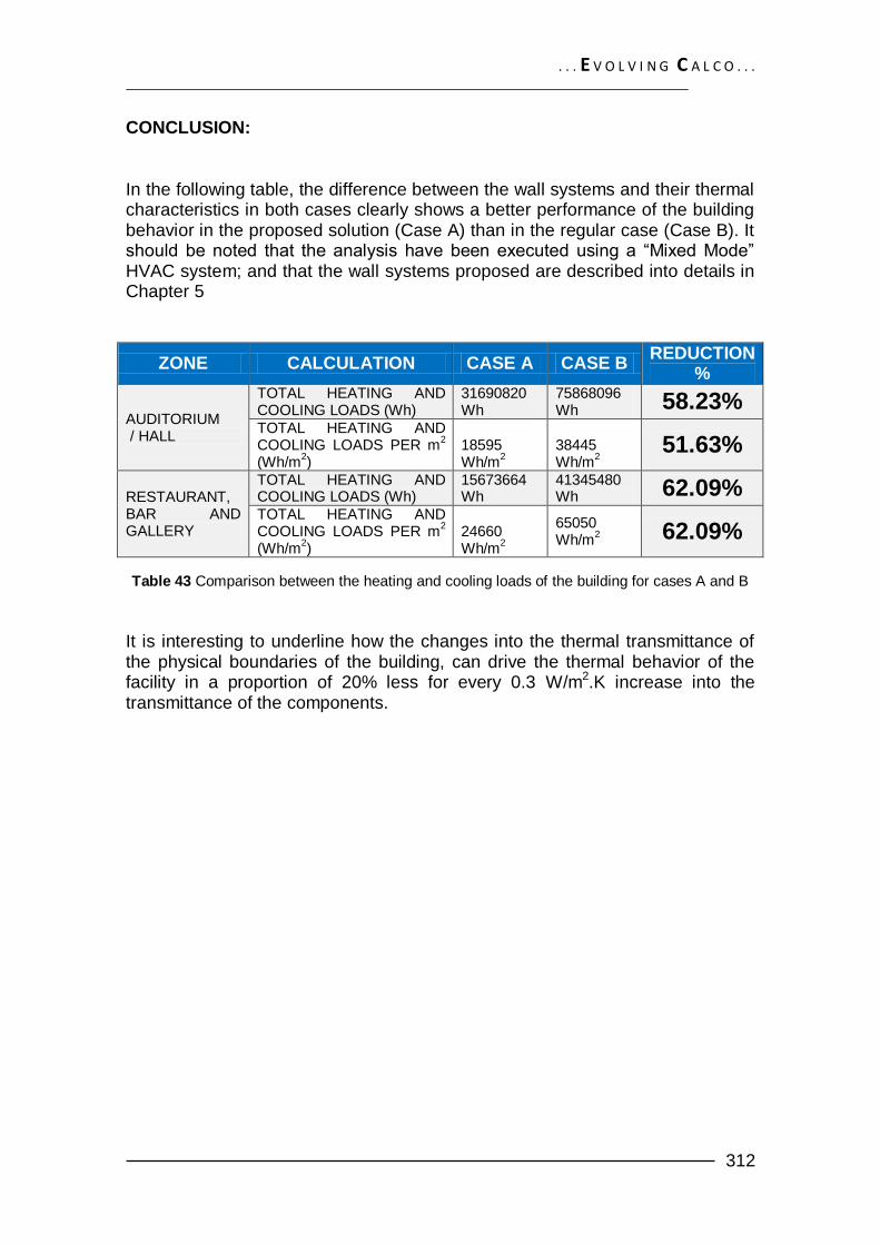
. . . E V O L V I N G C A L C O . . .

312

CONCLUSION:

In the following table, the difference between the wall systems and their thermal characteristics in both cases clearly shows a better performance of the building behavior in the proposed solution (Case A) than in the regular case (Case B). It should be noted that the analysis have been executed using a ―Mixed Mode‖ HVAC system; and that the wall systems proposed are described into details in Chapter 5

ZONE CALCULATION CASE A CASE B REDUCTION

%

AUDITORIUM / HALL

TOTAL HEATING AND COOLING LOADS (Wh)

31690820 Wh

75868096 Wh 58.23%

TOTAL HEATING AND COOLING LOADS PER m

2

(Wh/m2)

18595 Wh/m

2

38445 Wh/m

2

51.63%

RESTAURANT, BAR AND GALLERY

TOTAL HEATING AND COOLING LOADS (Wh)

15673664 Wh

41345480 Wh 62.09%

TOTAL HEATING AND COOLING LOADS PER m

2

(Wh/m2)

24660 Wh/m

2

65050 Wh/m

2 62.09%

Table 43 Comparison between the heating and cooling loads of the building for cases A and B

It is interesting to underline how the changes into the thermal transmittance of the physical boundaries of the building, can drive the thermal behavior of the facility in a proportion of 20% less for every 0.3 W/m2.K increase into the transmittance of the components.

. . . E V O L V I N G C A L C O . . .

313

7 HVAC SYSTEMS

7.1 METHODOLOGY The methodology for the estimation of the Heating, cooling loads and the system power is the one described by the ASHRAE (American Society of Heating, Refrigerating and Air-Conditioning Engineers).

7.2 SYSTEM SELECTION

The wide amount of uses that the structures will be holding, as well as the different internal loads and building envelope provided, makes indispensable the division of the project into two or more zones, which will have probably different ventilation systems that can satisfy the best solution in terms of energy saving. As a result, there are considered 5 heating zones distributed in two main buildings as follows: 7.2.1 Zone 1: Auditorium/hall

The solution consists on an HYBRID SYSTEM that comprises an all-air conditioning system supplying both heating and cooling needs for the space and natural ventilation powered by the fans of the air handling units. The system consists on an AHU that supplies the air conditioned into a cavity below the floor of the theater, which will regulate the velocity of air supply to the zone by means of floor-diffusers located approximately below the audience. According to the season and heating or cooling demands, the system will run by natural ventilation or air conditioning conditions. The system will consist on the next stages.

1. Intake and Air conditioning: the air handling unit at first will condition the external air to indoor temperature and humidity as required.

2. Supply: the air is supplied to a transition chamber right underneath the theater, reducing the velocity of the main duct supply needed for the correct ventilation and to avoid draughts or high velocities inside the conditioned zone.

3. Displacement ventilation: the air supplied to the zone will be heated up by the internal loads, being its density lower than the original fresh air coming from the bottom of the theater; the air will circulate to the top of the room where it will be extracted.

4. Extraction & recycling: the already preheated air by action of the sunspace cavity, outside the auditorium, will be mixed with the exhausted air coming from the space; a fan will redirect the mixed-air to the system after passing it by a heat exchanger, which will provide a profitable heat ―recycle‖ into the air conditioning system.

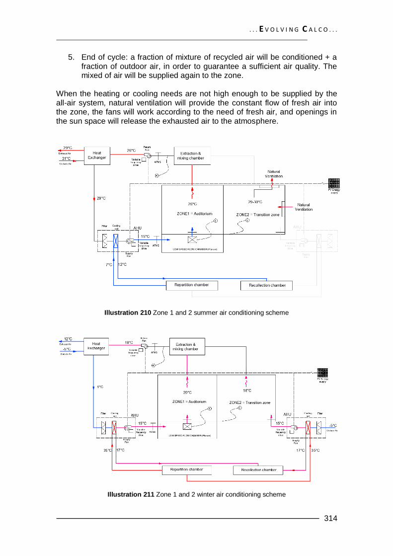
. . . E V O L V I N G C A L C O . . .

314

5. End of cycle: a fraction of mixture of recycled air will be conditioned + a fraction of outdoor air, in order to guarantee a sufficient air quality. The mixed of air will be supplied again to the zone.

When the heating or cooling needs are not high enough to be supplied by the all-air system, natural ventilation will provide the constant flow of fresh air into the zone, the fans will work according to the need of fresh air, and openings in the sun space will release the exhausted air to the atmosphere.

Illustration 210 Zone 1 and 2 summer air conditioning scheme

Illustration 211 Zone 1 and 2 winter air conditioning scheme

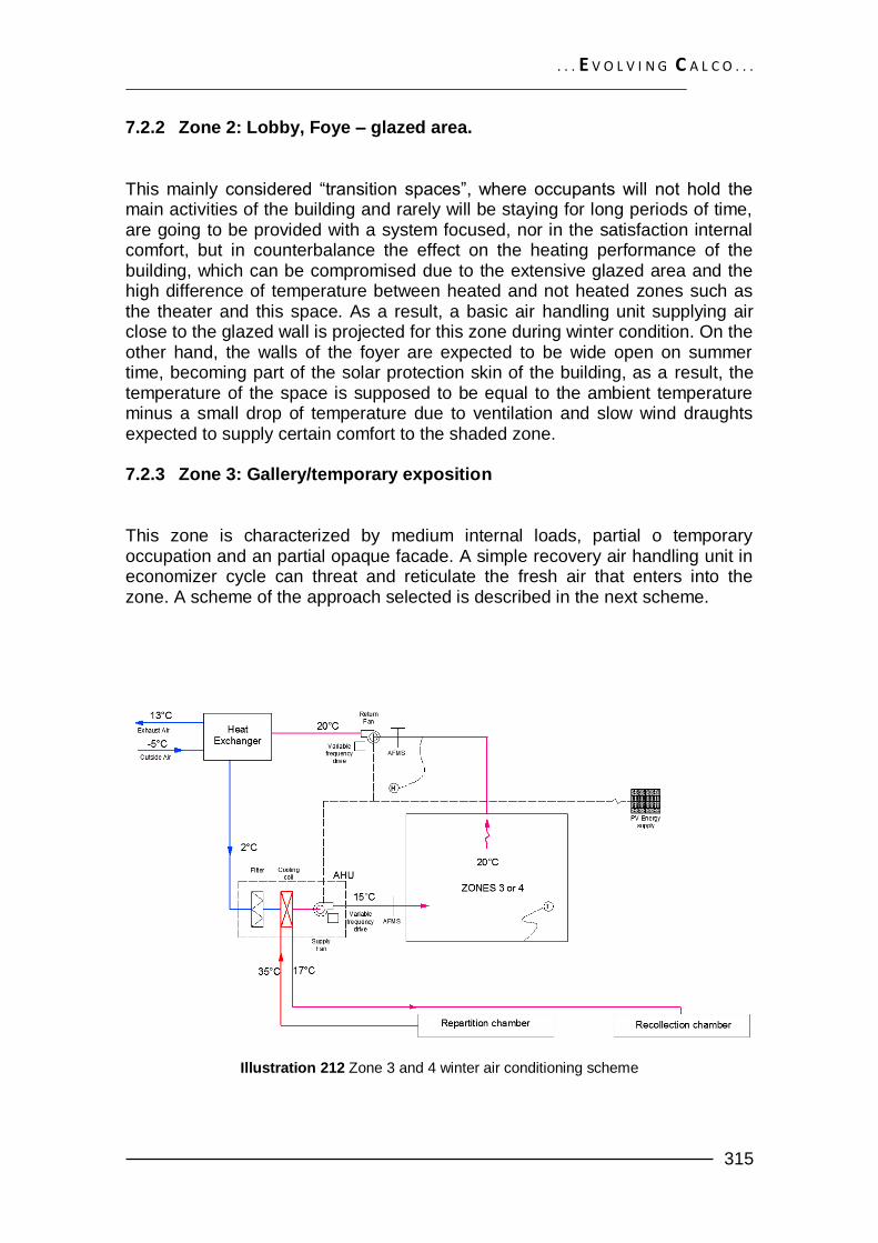
. . . E V O L V I N G C A L C O . . .

315

7.2.2 Zone 2: Lobby, Foye – glazed area.

This mainly considered ―transition spaces‖, where occupants will not hold the main activities of the building and rarely will be staying for long periods of time, are going to be provided with a system focused, nor in the satisfaction internal comfort, but in counterbalance the effect on the heating performance of the building, which can be compromised due to the extensive glazed area and the high difference of temperature between heated and not heated zones such as the theater and this space. As a result, a basic air handling unit supplying air close to the glazed wall is projected for this zone during winter condition. On the other hand, the walls of the foyer are expected to be wide open on summer time, becoming part of the solar protection skin of the building, as a result, the temperature of the space is supposed to be equal to the ambient temperature minus a small drop of temperature due to ventilation and slow wind draughts expected to supply certain comfort to the shaded zone. 7.2.3 Zone 3: Gallery/temporary exposition This zone is characterized by medium internal loads, partial o temporary occupation and an partial opaque facade. A simple recovery air handling unit in economizer cycle can threat and reticulate the fresh air that enters into the zone. A scheme of the approach selected is described in the next scheme.

Illustration 212 Zone 3 and 4 winter air conditioning scheme

. . . E V O L V I N G C A L C O . . .

316

Illustration 213 Zone 3 and 4 summer air conditioning scheme

7.2.4 Zone 4: Auditorium services areas. This zone is characterized by low internal loads, occupation and an entirely opaque façade. The same approach described above can be applied for this zone. 7.2.5 Zone 5: Restaurant/bars

This zone is characterized by medium to high constant occupancy in a partial- opaque façade. Different to the other zones, the restaurant and bars have a constant 8 hours per day running period, for which a system such as floor radiant panels can give the constant heating and cooling demand needed without long interrupting periods of operation. Natural ventilation will provide the air changes needed to maintain the air quality of the space

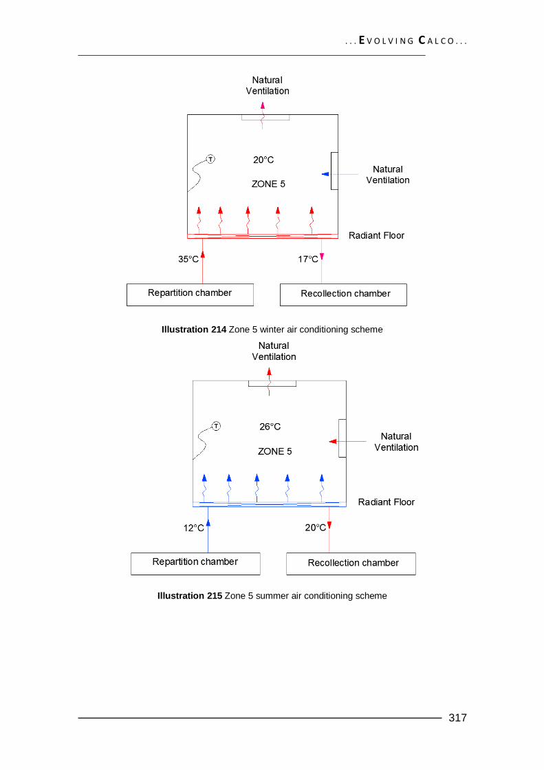
. . . E V O L V I N G C A L C O . . .

317

Illustration 214 Zone 5 winter air conditioning scheme

Illustration 215 Zone 5 summer air conditioning scheme

. . . E V O L V I N G C A L C O . . .

318

7.3 HVAC SYSTEM SIZING 7.3.1 Zone 1: Auditorium hall

People: 300 Approximated air volume: 2900 m3 considering an air tight building with minimum air infiltration rate According to the scheme established above, the size of the system will consist on getting the air flow rate passing throughout all the ducts and chambers, and then computing the area needed for a maximum velocity of 5 m/s for main ducts, and 0.5 m/s for the flow coming out through floor diffuser located above the low speed flow chamber. For air quality reasons it is considered a minimum air flow rate needed of Qmin =10 l/s per person and a Number of volume change rate between 6 and 10 ach.

122

So the flow should be increased:

As a result the main duct going out from the AHU will have the next dimensions:

Graphic 74 Main duct sizing and dimensions zone 1

122

GREENO, Roger; HALL, Fred. Building services handbook. 2007. P 159

. . . E V O L V I N G C A L C O . . .

319

On the other hand, the size of the plenum or low flow chamber can be obtained considering 0.4 m available of space under the floor of the theater (height) and the air flow intake to be equal to 0.5 m/s.

As a result, it has been decided to select parallel hanging rectangular ducts, interconnected to each other in order to achieve all the area needed.

Graphic 75 Plenum ducts system zone 1

Once the flow and diameters are obtained it is calculated the heating and cooling demands of energy due to ventilation. For Heating:

Equation 12 Heating load due to ventilation zone 1

For Cooling:

Equation 13 Cooling load due to ventilation zone 1

7.3.2 Zone 2: Lobby, Foye – glazed area.

People: 30 Approximated air volume: 4200 m3 considering an air tight building with minimum air infiltration rate For air quality reasons it is considered a minimum air flow rate needed of Qmin =10 l/s per person and a Number of volume change rate between 2 and 4 ach.

123

123


. . . E V O L V I N G C A L C O . . .

320

So the air flow should be increased:



Once the flow and section size are obtained it is calculated the heating and cooling demands of energy due to ventilation. For Heating:


7.3.3 Zone 3: Gallery/temporary exposition

People: 20 Approximated air volume: 1000 m3 considering an air tight building with minimum air infiltration rate For air quality reasons it is considered a minimum air flow rate needed of Qmin =10 l/s per person and a Number of volume change rate between 3 and 6 ach.124

124


. . . E V O L V I N G C A L C O . . .

321






For Cooling:


7.3.4 Zone 4: Auditorium Services areas People: 30

. . . E V O L V I N G C A L C O . . .

322

Approximated air volume: 1100 m3 considering an air tight building with minimum air infiltration rate. For air quality reasons it is considered a minimum air flow rate needed of Qmin =10 l/s per person and a Number of volume change rate between 3 and 6 ach.125






For Cooling:

125


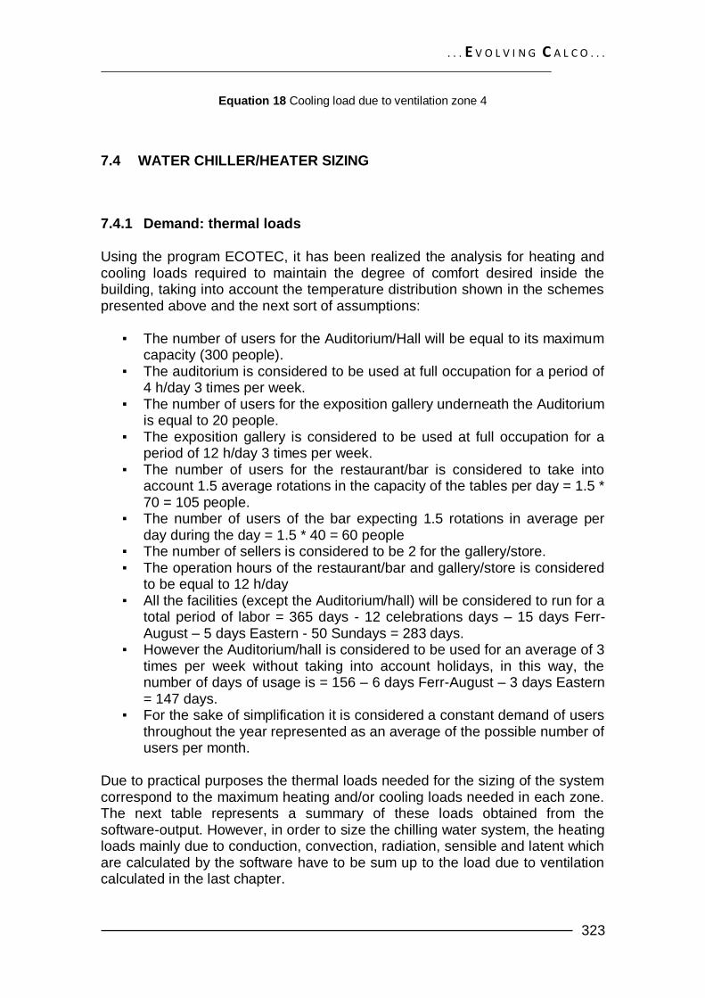
. . . E V O L V I N G C A L C O . . .

323


7.4 WATER CHILLER/HEATER SIZING

7.4.1 Demand: thermal loads

Using the program ECOTEC, it has been realized the analysis for heating and cooling loads required to maintain the degree of comfort desired inside the building, taking into account the temperature distribution shown in the schemes presented above and the next sort of assumptions:

▪ The number of users for the Auditorium/Hall will be equal to its maximum capacity (300 people).

▪ The auditorium is considered to be used at full occupation for a period of 4 h/day 3 times per week.

▪ The number of users for the exposition gallery underneath the Auditorium is equal to 20 people.

▪ The exposition gallery is considered to be used at full occupation for a period of 12 h/day 3 times per week.

▪ The number of users for the restaurant/bar is considered to take into account 1.5 average rotations in the capacity of the tables per day = 1.5 * 70 = 105 people.

▪ The number of users of the bar expecting 1.5 rotations in average per day during the day = 1.5 * 40 = 60 people

▪ The number of sellers is considered to be 2 for the gallery/store. ▪ The operation hours of the restaurant/bar and gallery/store is considered

to be equal to 12 h/day ▪ All the facilities (except the Auditorium/hall) will be considered to run for a

total period of labor = 365 days - 12 celebrations days – 15 days Ferr-August – 5 days Eastern - 50 Sundays = 283 days.

▪ However the Auditorium/hall is considered to be used for an average of 3 times per week without taking into account holidays, in this way, the number of days of usage is = 156 – 6 days Ferr-August – 3 days Eastern = 147 days.

▪ For the sake of simplification it is considered a constant demand of users throughout the year represented as an average of the possible number of users per month.

Due to practical purposes the thermal loads needed for the sizing of the system correspond to the maximum heating and/or cooling loads needed in each zone. The next table represents a summary of these loads obtained from the software-output. However, in order to size the chilling water system, the heating loads mainly due to conduction, convection, radiation, sensible and latent which are calculated by the software have to be sum up to the load due to ventilation calculated in the last chapter.

. . . E V O L V I N G C A L C O . . .

324

It is supposed (as it was previously stated) that the system will chill and store the dairy cold water demand running at full capacity during night (when the electrical fees are lower) and during day.

Table 44 Summary of diary peak thermal loads

7.4.2 Sizing The sizing of the chilled water tank storage is done by calculating the chilling capacity needed in order to attend the cooling demand. The next equation is employed to attain this scope considering that the chiller will be running in off-peak periods at full capacity. (12h.day). For cooling:

For heating:

In these order of ideas, the chilled water storage is sized according to the heat capacity of the water and the considered efficiency of the system (in this case, a simple insulated water tank storage), thus:

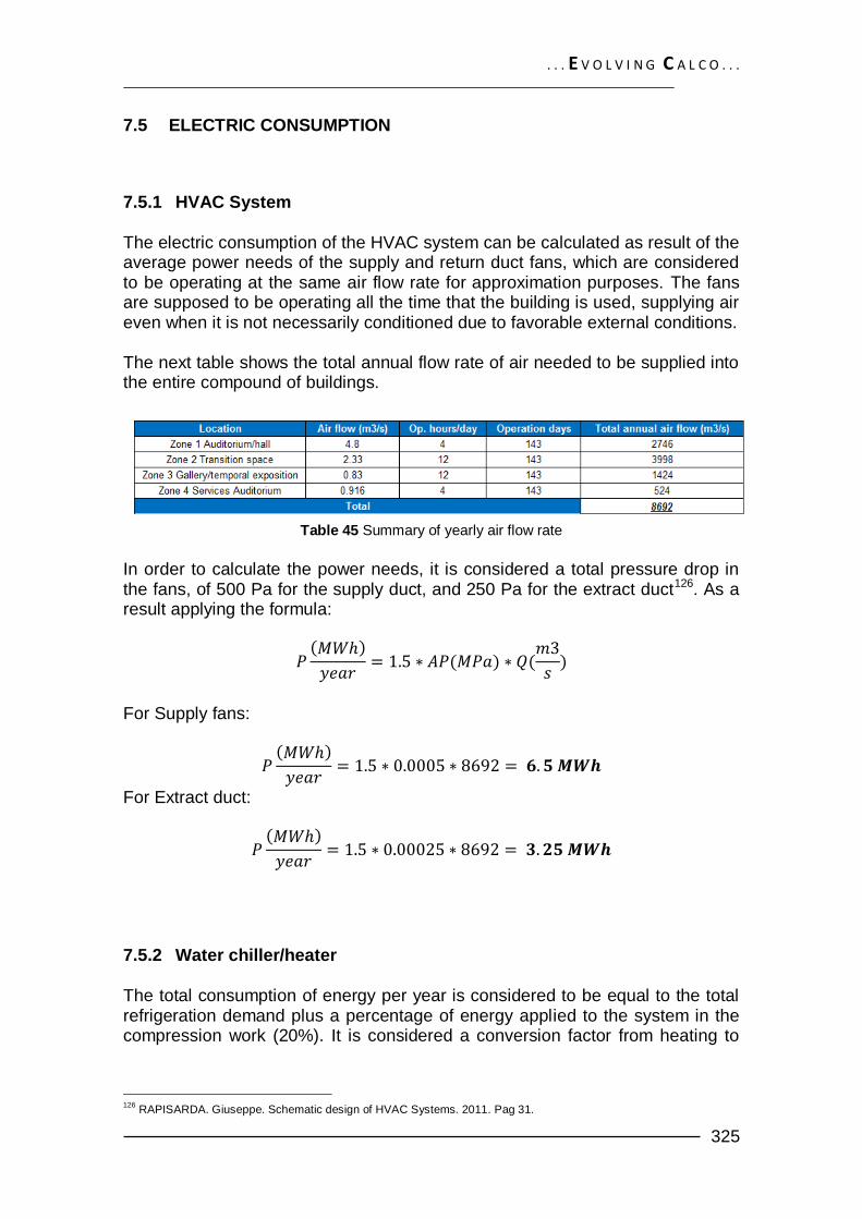
. . . E V O L V I N G C A L C O . . .

325

7.5 ELECTRIC CONSUMPTION

7.5.1 HVAC System The electric consumption of the HVAC system can be calculated as result of the average power needs of the supply and return duct fans, which are considered to be operating at the same air flow rate for approximation purposes. The fans are supposed to be operating all the time that the building is used, supplying air even when it is not necessarily conditioned due to favorable external conditions. The next table shows the total annual flow rate of air needed to be supplied into the entire compound of buildings.

Table 45 Summary of yearly air flow rate

In order to calculate the power needs, it is considered a total pressure drop in the fans, of 500 Pa for the supply duct, and 250 Pa for the extract duct126. As a result applying the formula:

For Supply fans:

For Extract duct:

7.5.2 Water chiller/heater

The total consumption of energy per year is considered to be equal to the total refrigeration demand plus a percentage of energy applied to the system in the compression work (20%). It is considered a conversion factor from heating to

126

RAPISARDA. Giuseppe. Schematic design of HVAC Systems. 2011. Pag 31.

. . . E V O L V I N G C A L C O . . .

326

electrical energy needs equal to 0.4. The next table shows the total refrigeration demand per year in the compound of buildings.

Table 46 Summary of annual thermal loads

As a result the electrical consumption of the water chiller/heater is equal to

49*1.2*0.4 = 24 MWh/year

. . . E V O L V I N G C A L C O . . .

327

8 GEOTHERMAL HEAT PUMP ENERGY

8.1 METHODOLOGY The selection and design of the system is oriented to obtain the flow rate of ground water needed in order to supply the heating and cooling demand of the building. Once the flow rate is obtained, it can be sized the number of wells, piping size and the electrical energy needed for pumping.

8.2 SYSTEM SELECTION According to historical and geomorpholic data available for the area of San Vigilio, the project’s zone is characterized by the presence of a constant running water body located at 2 m below ground level. The presence of a water body right in the boundaries of the project, constitute a high opportunity to apply an OPEN LOOP SYSTEM which requires basically an intake minimum of 10 m in order to avoid freezing or changes in the temperature of ground according to the season; other systems such as the closed loop systems will required more area (horizontal systems) or drilling depth (vertical systems) which would increase considerably the initial cost of installation and subsequent operation costs due to maintenance. Due to the size of the building and zones distribution, it has been decided to use (2) two independent open loop systems to supply ground heat to the project, 1 for the zones 1,2,3 and another one for the zones 3 and 4. On more important consideration is the inclusion of a chilled water storage system for the zones 3 and 4, knowing that a saving energy strategy in the case of high cooling loads can be achieved by cooling the on-day demand of chilled water in non-peak times (at night) running the system at full capacity, when the electrical fees are lower.

Illustration 216. Winter Heating energy system supply

. . . E V O L V I N G C A L C O . . .

328

Illustration 217. Summer cooling energy system supply

On the other hand, the use of ground heating pumping for supplying the needs of hot water to the restaurant can be established as it is indicated in the next scheme: 8.2.1 Water heating pump wells The system will be composed by a production well and injection well, in which

running water at a constant temperature of 12C127 will be extracted from the water body and then released to it after a heat exchange process is run throughout the system. In order to avoid serious problems caused by circulating groundwater directly to the building, the energy provided by the well pumping is extracted by a heat exchanger where ―Clean water‖ will absorb (Heating cycle) or release energy (Cooling cycle) towards and/or from the main system circuit. In the next set of graphics it is shown a basic plan of the water heat pump wells connection to the main heating and cooling system of the building.

127

MCQUAY International. Geothermal Heat pump design manual. Application guide. Appendix 1: Ground

temperatures. Heating and cooling with a heat pump. 2011. p 38

. . . E V O L V I N G C A L C O . . .

329

Illustration 218. Winter water heating source plan

Illustration 219. Summer water heating source plan

8.2.2 Ground water heating/chilling units128

In the heating cycle, the water/refrigerant which has absorbed heat energy form the ground water is transported to the (GWHU) existing in each one of the zones of the building, the water boils to become a low-temperature vapor; a reversing valve then sends the refrigerant vapor to the compressor. The vapor is then compressed which reduces its volume, causing it to heat up, the excess of heat is taken by a desuperheater. A desuperheater is a small, auxiliary heat exchanger that uses superheated gases from the heat pump's compressor to heat water, this hot water then circulates through a pipe to the storage water heater tank. Finally, the reversing valve sends the now-hot gas to the condenser coil, where it gives up its heat. Water passes across the coil, heated, and supplied to the air handling units or under floor panels. Given up its heat, the refrigerant passes through the expansion valve, where its temperature and

128

NATURAL RESOURCES OF CANADA. Heating and cooling with a heat pump. 2011 (Available on-line),

ttp://oee.nrcan.gc.ca/publications/infosource/pub/home/ Heating_and_Cooling _with_a_Heat_Pump_Section4.cfm

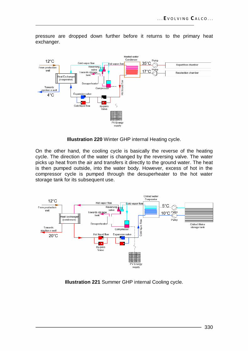
. . . E V O L V I N G C A L C O . . .

330

pressure are dropped down further before it returns to the primary heat exchanger.

Illustration 220 Winter GHP internal Heating cycle.

On the other hand, the cooling cycle is basically the reverse of the heating cycle. The direction of the water is changed by the reversing valve. The water picks up heat from the air and transfers it directly to the ground water. The heat is then pumped outside, into the water body. However, excess of hot in the compressor cycle is pumped through the desuperheater to the hot water storage tank for its subsequent use.

Illustration 221 Summer GHP internal Cooling cycle.

. . . E V O L V I N G C A L C O . . .

331

8.3 SIZING The sizing of the systems consists basically on the capacity of the appliances to pump the required flow of energy of the chiller/heater. This value can be obtained by means of computation between the energy flow throughout the system, and the difference in temperatures of the process intake and outtake. For this application, the peak value of chilling/heating water capacity will drive the size of the geothermal pump. Hence, taking into consideration the water heater/chilling unit maximum capacity = 40 kW. (as it was presented in the last chapter) , and a difference of

temperature between the extraction and injection wells of 8C, the total pumping flow required is equal to:

Thus, a heating pump that can supply water to 8434 l/h is used for the described application.

8.4 ELECTRICAL CONSUMPTION The electrical consumption of the open loop ground heating pump can be estimated by calculating the flow demand of the pump and its consequent electric consumption throughout the year. As a result, taking into consideration an annual heating and cooling load requirement of 40.4 MWh and 8.33 MWh, (as it was presented in the last chapter) , and a difference of temperature between the extraction and injection

wells of 8C, the total pumping flow per year required is equal to: During heating season:

During cooling season:

. . . E V O L V I N G C A L C O . . .

332

With these results the electrical consumption of the pumping unit can be approximated considering an average 0.6 efficiency along the year, and a head of pressure equal to the height of the perforation well (10m) plus 20% for losses due to friction:

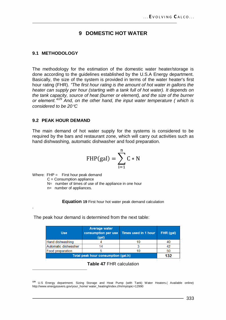
. . . E V O L V I N G C A L C O . . .

333

9 DOMESTIC HOT WATER

9.1 METHODOLOGY The methodology for the estimation of the domestic water heater/storage is done according to the guidelines established by the U.S.A Energy department. Basically, the size of the system is provided in terms of the water heater's first hour rating (FHR). “The first hour rating is the amount of hot water in gallons the heater can supply per hour (starting with a tank full of hot water). It depends on the tank capacity, source of heat (burner or element), and the size of the burner or element.”129 And, on the other hand, the input water temperature ( which is

considered to be 20C

9.2 PEAK HOUR DEMAND The main demand of hot water supply for the systems is considered to be required by the bars and restaurant zone, which will carry out activities such as hand dishwashing, automatic dishwasher and food preparation.

Where: FHP = First hour peak demand C = Consumption appliance N= number of times of use of the appliance in one hour n= number of appliances.

Equation 19 First hour hot water peak demand calculation

. The peak hour demand is determined from the next table:

Table 47 FHR calculation

129 U.S Energy department. Sizing Storage and Heat Pump (with Tank) Water Heaters.( Available online)

http://www.energysavers.gov/your_home/ water_heating/index.cfm/mytopic=12990

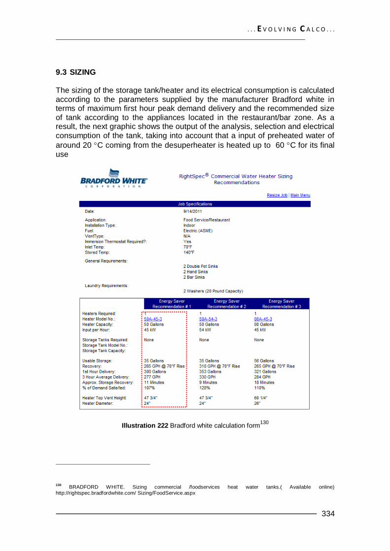
. . . E V O L V I N G C A L C O . . .

334

9.3 SIZING The sizing of the storage tank/heater and its electrical consumption is calculated according to the parameters supplied by the manufacturer Bradford white in terms of maximum first hour peak demand delivery and the recommended size of tank according to the appliances located in the restaurant/bar zone. As a result, the next graphic shows the output of the analysis, selection and electrical consumption of the tank, taking into account that a input of preheated water of

around 20 C coming from the desuperheater is heated up to 60 C for its final use

Illustration 222 Bradford white calculation form130

130 BRADFORD WHITE. Sizing commercial /foodservices heat water tanks.( Available online)

http://rightspec.bradfordwhite.com/ Sizing/FoodService.aspx

http://rightspec.bradfordwhite.com/

. . . E V O L V I N G C A L C O . . .

335

9.4 ELECTRICAL CONSUMPTION Choosing a water storage/heater electric tank with an input power of 45 kWh used half an hour per day to produce the total heating need, during operation time of the bar/restaurant facilities (283 days) a total electrical consumption per year equal to 45*0.5*283 = 6.2 MWh/year.

On the other hand, if we analyze the behavior of the system in terms of energy consumption by considering the no use of a desuperheater, and thus having a

typical intake of water at 5C. we would obtain a consumption equal to 57*0.5*283 = 8 MWh/year. Hence it can be inferred an electrical energy saving of 1.8 Mwh/year only using a desuperheater appliance.

. . . E V O L V I N G C A L C O . . .

336

Illustration 223 Bradford white calculation form without desuperheater

131

131 BRADFORD WHITE. Sizing commercial /foodservices heat water tanks.( Available online)

http://rightspec.bradfordwhite.com/ Sizing/FoodService.aspx


. . . E V O L V I N G C A L C O . . .

337

10 SOLAR PHOTOVOLTAIC SYSTEM

10.1 METHODOLOGY The methodology for the estimation of the electrical energy production given by the system is the one indicated by the Joint Research center of the European commission. In general the system is planned to produce equal but not more than the energy required, in order to be able to consume all the energy needed, and sell the less possible to the electrical grid (which payback is less than the obtained by consuming energy).

10.2 SYSTEM SELECTION According to facts analyzed in the chapter ―strategies‖, and the areas available for the positioning array of solar photovoltaic panels, it has be chosen a system of free-standing monocrystalline silicon PV panels that can be projected for the areas over the roof of the Auditorium/Hall and the parking spaces at an

optimum inclination angle of 39 towards south. The photovoltaic arrange will provide the electric demand to the appliances throughout the all building. Taking into account the low reliability of the system to be able to accumulate and supply the whole energy to the building constantly, a grid-connected system is proposed in order to obtain the necessary energy from the grid in winter conditions (out of the one utilized from solar radiation), and export the overflow of energy in summer when solar radiation is higher and the battery storage is full.

. . . E V O L V I N G C A L C O . . .

338

Illustration 224 Photovoltaic system scheme.

The maximum energy that can be produced by this kind of panels is considered to be 1kWp per every 8 m2.

10.3 ENERGY DEMANDS

The electrical energy demands considered are obtained from the results presented in the last chapters. However, electrical consumptions that are not measured and are outside of the scope of the present analysis (I.e lighting, electrical appliances) are hence estimated:

Table 48 Miscellaneous and lighting electrical energy estimated consumption

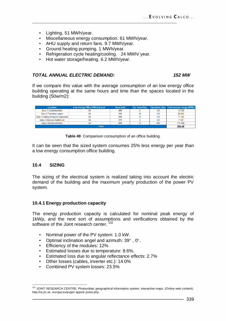
. . . E V O L V I N G C A L C O . . .

339

▪ Lighting. 51 MWh/year. ▪ Miscellaneous energy consumption. 61 MWh/year. ▪ AHU supply and return fans. 9.7 MWh/year. ▪ Ground heating pumping. 1 MWh/year. ▪ Refrigeration cycle heating/cooling. 24 MWh/ year. ▪ Hot water storage/heating. 6.2 MWh/year.

TOTAL ANNUAL ELECTRIC DEMAND: 152 MW If we compare this value with the average consumption of an low energy office building operating at the same hours and time than the spaces located in the building (50w/m2):

Table 49 Comparison consumption of an office building.

It can be seen that the sized system consumes 25% less energy per year than a low energy consumption office building.

10.4 SIZING

The sizing of the electrical system is realized taking into account the electric demand of the building and the maximum yearly production of the power PV system. 10.4.1 Energy production capacity

The energy production capacity is calculated for nominal peak energy of 1kWp, and the next sort of assumptions and verifications obtained by the software of the Joint research center. 132

▪ Nominal power of the PV system: 1.0 kW.

▪ Optimal inclination angel and azimuth: 39 , 0. ▪ Efficiency of the modules: 12% ▪ Estimated losses due to temperature: 8.6%. ▪ Estimated loss due to angular reflectance effects: 2.7% ▪ Other losses (cables, inverter etc.): 14.0% ▪ Combined PV system losses: 23.5%

132

JOINT RESEARCH CENTRE. Photovoltaic geographical information system, interactive maps. (Online web content).

http://re.jrc.ec. europa.eu/pvgis/ apps4/ pvest.php

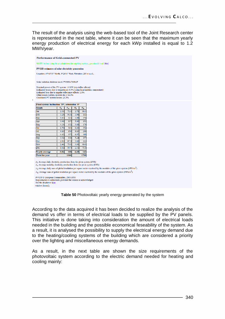
. . . E V O L V I N G C A L C O . . .

340

The result of the analysis using the web-based tool of the Joint Research center is represented in the next table, where it can be seen that the maximum yearly energy production of electrical energy for each kWp installed is equal to 1.2 MWh/year.

,

Table 50 Photovoltaic yearly energy generated by the system

According to the data acquired it has been decided to realize the analysis of the demand vs offer in terms of electrical loads to be supplied by the PV panels. This initiative is done taking into consideration the amount of electrical loads needed in the building and the possible economical feseability of the system. As a result, it is analysed the possibility to supply the electrical energy demand due to the heating/cooling systems of the building which are considered a priority over the lighting and miscellaneous energy demands. As a result, in the next table are shown the size requirements of the photovoltaic system according to the electric demand needed for heating and cooling mainly:

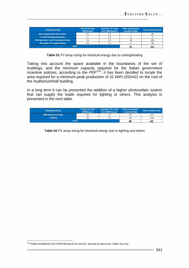
. . . E V O L V I N G C A L C O . . .

341

Table 51 PV array sizing for electrical energy due to cooling/heating Taking into account the space available in the boundaries of the set of buildings, and the minimum capacity required for the Italian government incentive policies, according to the PEP133. it has been decided to locate the area required for a minimum peak production of 31 kWh (252m2) on the roof of the Auditorium/hall building. In a long term it can be presented the addition of a higher photovoltaic system that can supply the loads required for lighting or others. This analysis is presented in the next table.

Table 52 PV array sizing for electrical energy due to lighting and others

133

PIANO ENERGETICO PROVINCIALE DI LECCO. Scheda di Intervento. 2009. Pg 4:44.

. . . E V O L V I N G C A L C O . . .

342

11 ACOUSTICAL SYSTEM

11.1 METHODOLOGY The calculation process has been done taking into account the instances and material properties obtained from different manufacturers of panels and the standard UNI 12354. For the sake of simplicity, and taking into account the expected use and size of the theater/ auditorium, it has been considered to evaluate the reverberation time of the space as a measurement of the quality of sound that the space will present in a concert, speech-theater or any other multipurpose activity at small scale.

11.2 SYSTEM SELECTION

Multi-purpose uses, demands that auditorium acoustics satisfy acoustical needs for theatrical performances, concerts, speeches, assemblies, and public gatherings equally well. The auditorium context designed for a capacity of 300 seats can be seen as a minimum area to realize high efficient acoustical performance, however, some considerations about internal acoustic insulation and straight perforated panels on roof and walls can enhance the brightness and warmth of the sound around the hall. It has to be considered that in most of the cases conflicting requirements can occur between the different activities for which the room is conditioned, due to the main objectives that a concert or on the other hand a speech are trying to attain in the room. In particular terms, the acoustics of a space designed for mainly speech activities must ensure basically the intelligibility, definition and understanding in the gestural and vocal communication process carried out in the room, as a result, it can be considered that the quality of the speech signal is not too critical, as long as the speaker’s voice and accent are recognizable. On the other hand, music audiences are expecting for good qualities of sound for various styles of music, while the clarity and recognition is not influent considered influent in the performance and it is considered to give the impression of brittleness or dryness in the act, by also giving low levels of brightness, which is required in a concert. Another crucial difference between this two activities is that music can consist of a great range of frequencies (20 Hz – 20 kHz) while speech mainly occurs at a narrow band signal (500 Hz – 4kHz). Taking into account the conditions stated above, it has been considered to use the next compound of systems to produce the dynamic behavior of the multipurpose auditorium/hall. 11.2.1 Absorbers

. . . E V O L V I N G C A L C O . . .

343

In order to provide the necessary sound absorption for the multipurpose auditorium/hall, it has been proposed a layered scheme of the main absorbing walls, giving the flexibility to the inclusion or exclusion of absorptive material ( fiberglass) depending on the need of the design, while keeping the architectural finishing of the room. The location of the absorbers in the room will be around all the perimeter of the vertical walls of the room.

Graphic 79 Absorber-wall scheme- with and without fiberglass layer. (Extracted from Wiener)

134

11.2.2 Reflectors

The hanging reflectors to be located into the auditorium are meant to produce the maximum reflection of the first waves produced to the audience form and to all the parts of the room. The reflectors will be mainly located in the ceiling of the auditorium starting from the end line of the stage towards the end line of the backseats. 11.2.3 Rotating panels Being one of the simplest types of appliances that can be used and fit into the design of the building, it has been chosen a dynamic system that can reproduce the levels of reflection and absorption desired during each activity to be performed. As a result, the operation of the panels will generate the required reverberation times for a theatrical/recital/musical activity when the absorber face is close, letting a maximum reflection that can enhance the sound quality of these activities. On the other hand, when the rotating panels are wide open, (absorber face open) the level of absorption will rise, lowering the reverberation time of the room, which is a need in order to obtain the balance sound in the narrow band signal of a speech activity. The location of these panels will be on

134

Wiener, Ethan. Acoustic treatment and design for listening rooms and recording studios. A [ Available online]. http://www.ethanwiner.com/acoustics.html

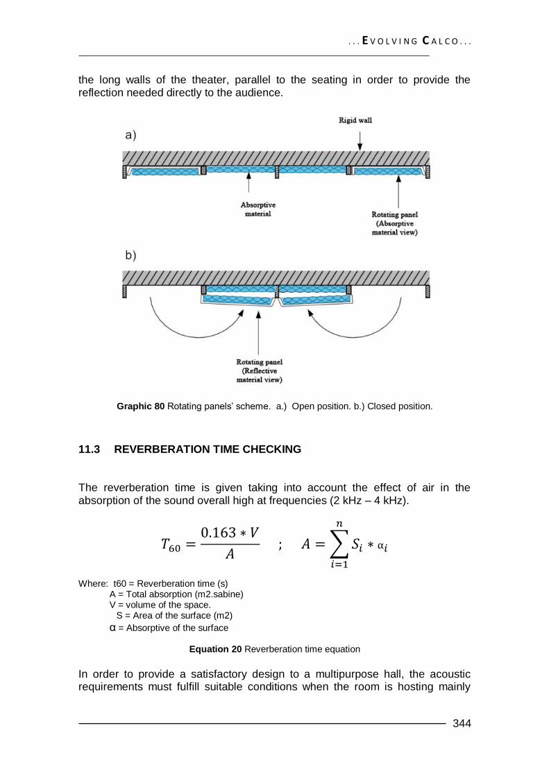
. . . E V O L V I N G C A L C O . . .

344

the long walls of the theater, parallel to the seating in order to provide the reflection needed directly to the audience.

Graphic 80 Rotating panels’ scheme. a.) Open position. b.) Closed position.

11.3 REVERBERATION TIME CHECKING The reverberation time is given taking into account the effect of air in the absorption of the sound overall high at frequencies (2 kHz – 4 kHz).

Where: t60 = Reverberation time (s) A = Total absorption (m2.sabine) V = volume of the space.

S = Area of the surface (m2)

α = Absorptive of the surface

Equation 20 Reverberation time equation

In order to provide a satisfactory design to a multipurpose hall, the acoustic requirements must fulfill suitable conditions when the room is hosting mainly

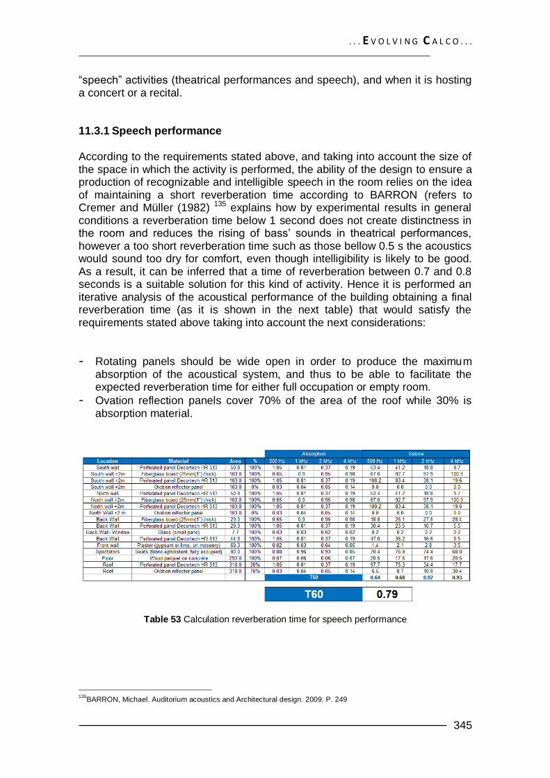
. . . E V O L V I N G C A L C O . . .

345

―speech‖ activities (theatrical performances and speech), and when it is hosting a concert or a recital. 11.3.1 Speech performance

According to the requirements stated above, and taking into account the size of the space in which the activity is performed, the ability of the design to ensure a production of recognizable and intelligible speech in the room relies on the idea of maintaining a short reverberation time according to BARRON (refers to Cremer and Müller (1982) 135 explains how by experimental results in general conditions a reverberation time below 1 second does not create distinctness in the room and reduces the rising of bass’ sounds in theatrical performances, however a too short reverberation time such as those bellow 0.5 s the acoustics would sound too dry for comfort, even though intelligibility is likely to be good. As a result, it can be inferred that a time of reverberation between 0.7 and 0.8 seconds is a suitable solution for this kind of activity. Hence it is performed an iterative analysis of the acoustical performance of the building obtaining a final reverberation time (as it is shown in the next table) that would satisfy the requirements stated above taking into account the next considerations:

- Rotating panels should be wide open in order to produce the maximum absorption of the acoustical system, and thus to be able to facilitate the expected reverberation time for either full occupation or empty room.

- Ovation reflection panels cover 70% of the area of the roof while 30% is absorption material.

Table 53 Calculation reverberation time for speech performance

135

BARRON, Michael. Auditorium acoustics and Architectural design. 2009. P. 249

. . . E V O L V I N G C A L C O . . .

346

11.3.2 Musical performance

The reverberation time of spaces such as the one considered in the present project can be considered to be similar to the one required for a small recital hall which can differ from the one needed for a big opera house/theater or concert halls basically on its capacity. As an example, the reverberation time for symphony concert halls is a function of the ―programme‖ only, while smaller halls depend directly, or are more sensitive to the volume of the space as a result of an empirical application. Recommendations in the design of small halls find suitable the use of a reverberation time between 1.4 – 1.7 for a volume of up to 3000 m3. Hence it is performed an iterative analysis of the acoustical performance of the building obtaining a final reverberation time (as it is shown in the next table) that would satisfy the requirements stated above taking into account the next considerations:

- Rotating panels should be closed in order to produce the minimum absorption of the acoustical system, and thus to be able to facilitate the expected reverberation time for either full occupation or empty room.

- Ovation reflection panels cover 70% of the area of the roof while 30% is absorption material.

Table 54 Calculation reverberation time for speech performance

. . . E V O L V I N G C A L C O . . .

347

12 RAIN WATER RECOLLECTION SYSTEM

12.1 METHODOLOGY The following calculation is made according to the data presented in the last chapter regarding characteristic monthly average precipitation rates for the zone of the project, and following the methodology described in the Rainwater tank harvesting anual136 and the Texas137 rain water harvesting manuals. For

simplification purposes, and given the level of detail to be produced at the end of this work, the theory is assumed to be concise for feasibility purposes, although factors such as evaporation rates, wind velocity and other parameters are not estimated as an influence in the design, but however it has been demonstrated that can influence real efficiency of a system. For estimating demands it has been decided to use the instances purposed by the Water System design Manual.138 On the other hand, the design of gutters has been done following the instances given by the standard UNI EN 12056 – 3 – Sistemi per l’evacuazione delle acque meteoriche, progettazione e calcolo.

12.2 SCHEMATIC DESIGN

The design of the rain water recollection systems consists of 2 parts: a catching system composed by a series of gutters that recollect the rain water coming from the available roof area, a second part consist on an storage system that will supply the water by means of gravity to each one of the toilet rooms existing in the compound of buildings. In the next series of graphic it is shown the system complexity.

136

THE CABELL BRAN CENTER Virginia Rainwater tank harvesting manual. 2007. P33. 137

TEXAS WATER DEVELOPMENT BOARD. The texas Manual on rainwater harvesting. 2005. P32. 138

WASHINGTON STATE DEPARTMENT OF HEALTH. Water System design Manual. 2009. P37-38

. . . E V O L V I N G C A L C O . . .

348

Illustration 225 Auditorium/hall water catching system - gutters and channels

scheme

Illustration 226 Restaurant/bar water catching system - gutters and channels scheme

According to the area of the building, it has been estimated that the water catching area available be reduced up to the point in which it can be satisfied

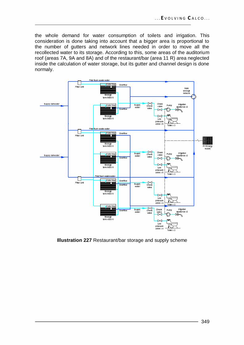
. . . E V O L V I N G C A L C O . . .

349

the whole demand for water consumption of toilets and irrigation. This consideration is done taking into account that a bigger area is proportional to the number of gutters and network lines needed in order to move all the recollected water to its storage. According to this, some areas of the auditorium roof (areas 7A, 9A and 8A) and of the restaurant/bar (area 11 R) area neglected inside the calculation of water storage, but its gutter and channel design is done normaly.

Illustration 227 Restaurant/bar storage and supply scheme

. . . E V O L V I N G C A L C O . . .

350

Illustration 228 Auditorium/hall storage and supply scheme

12.3 CHANNELS DESIGN 12.3.1 Sizing: The sizing of channels is given according to the different geometry and distribution water catching areas throughout the roof of the compound of buildings. In the next graphic it is shown the catchment areas which are adjacent to the channels for its sizing.

Illustration 229 channels distribution in the building (roof - plan view)

. . . E V O L V I N G C A L C O . . .

351

Graphic 81. Sizing of rainfall catching channels.

12.3.2 Rainwater demand

The demand of rainfall water for the gutters and channels is calculated independently for each one of the buildings that compose the project (Auditorium/hall, Restaurant/bar) as well as it has been done for the storage capacity calculation. The value obtained of the demand should be assessed against the capacity of the channels in order to obtain its size and specific dimensions:

Where: Q = demand of the system to transport r = Raining intensity. (l/s*m2), k = risk coefficient ( when r’ cannot be calculated by statistical methods. A= Effective roof area (m2) C= runoff coefficient = 1

Equation 21 Expected demand of the system.

Taking into account the impossibility to calculate for statistical methods the rainfall intensity, it has been chosen a conservative value of rainfall intensity r = 0.05 l/m2.s times a k coefficient = 2, due to the high amount of channels inside the boundaries of the building. However, for the channels of the roof in ETFE which are considered to be outside of the structure, k = 1.

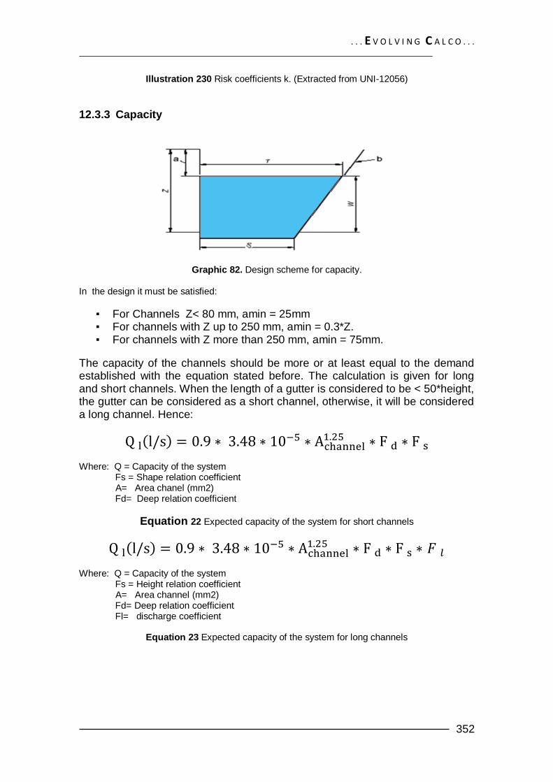
. . . E V O L V I N G C A L C O . . .

352

Illustration 230 Risk coefficients k. (Extracted from UNI-12056)

12.3.3 Capacity

Graphic 82. Design scheme for capacity.

In the design it must be satisfied:

▪ For Channels Z< 80 mm, amin = 25mm ▪ For channels with Z up to 250 mm, amin = 0.3*Z. ▪ For channels with Z more than 250 mm, amin = 75mm.

The capacity of the channels should be more or at least equal to the demand established with the equation stated before. The calculation is given for long and short channels. When the length of a gutter is considered to be < 50*height, the gutter can be considered as a short channel, otherwise, it will be considered a long channel. Hence:

Where: Q = Capacity of the system Fs = Shape relation coefficient A= Area chanel (mm2) Fd= Deep relation coefficient

Equation 22 Expected capacity of the system for short channels

Where: Q = Capacity of the system Fs = Height relation coefficient A= Area channel (mm2) Fd= Deep relation coefficient Fl= discharge coefficient

Equation 23 Expected capacity of the system for long channels

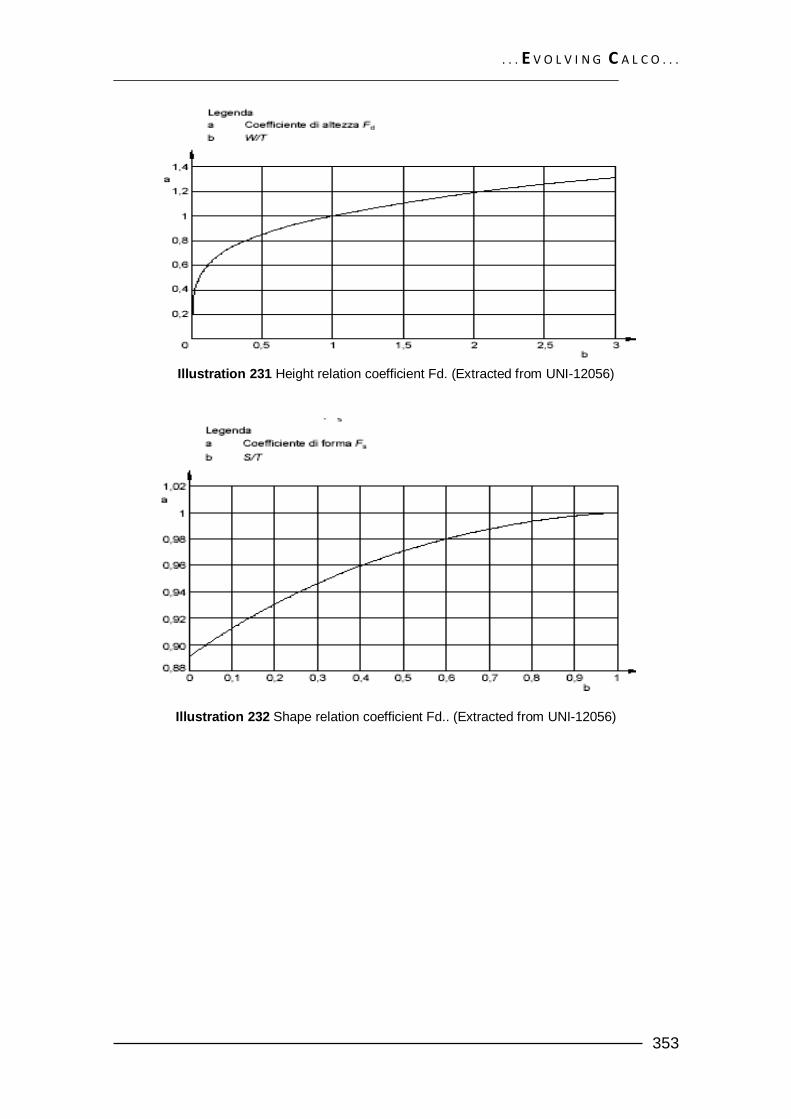
. . . E V O L V I N G C A L C O . . .

353

Illustration 231 Height relation coefficient Fd. (Extracted from UNI-12056)

Illustration 232 Shape relation coefficient Fd.. (Extracted from UNI-12056)

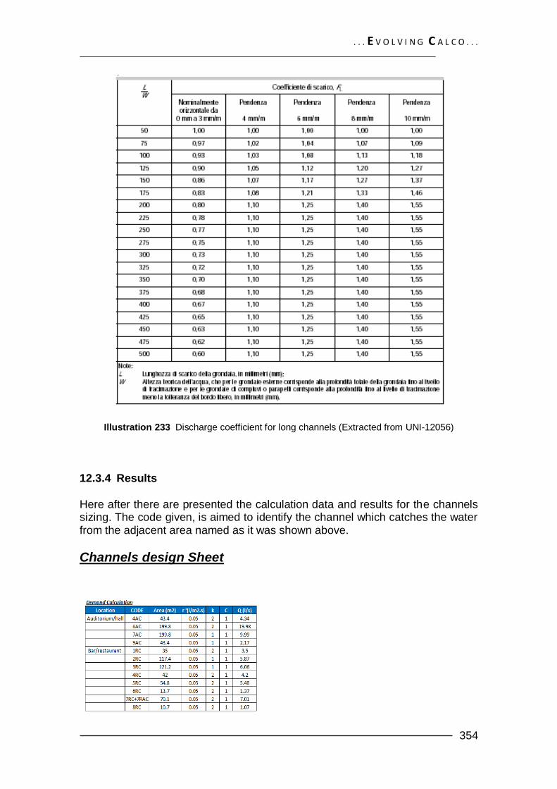
. . . E V O L V I N G C A L C O . . .

354

Illustration 233 Discharge coefficient for long channels (Extracted from UNI-12056)

12.3.4 Results Here after there are presented the calculation data and results for the channels sizing. The code given, is aimed to identify the channel which catches the water from the adjacent area named as it was shown above.

Channels design Sheet

. . . E V O L V I N G C A L C O . . .

355

12.4 GUTTERS DESIGN 12.4.1 Sizing: The sizing of vertical gutters is given according to the different geometry and distribution of the water catching areas throughout the roof. In the next graphic it is shown the catchment areas which supply the water demand to the gutter. For simplification purposes the gutters nomenclature will be given according to its adjacent area.

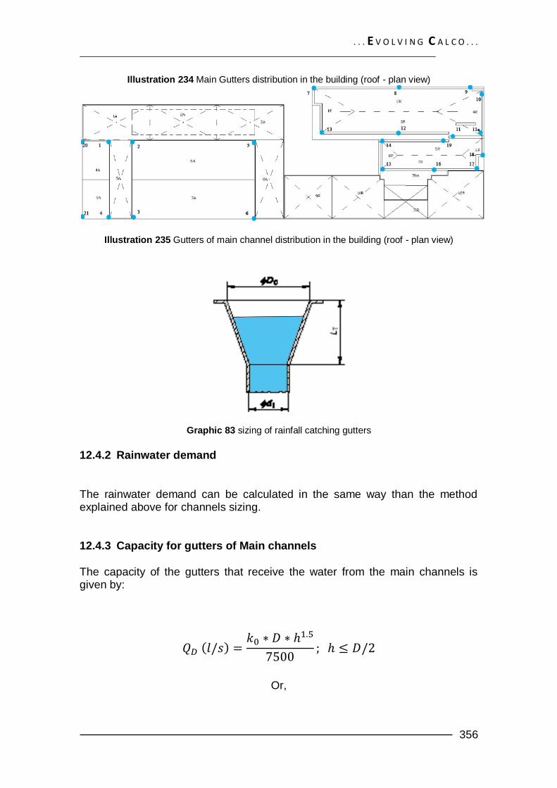
. . . E V O L V I N G C A L C O . . .

356

Illustration 234 Main Gutters distribution in the building (roof - plan view)

Illustration 235 Gutters of main channel distribution in the building (roof - plan view)

Graphic 83 sizing of rainfall catching gutters

12.4.2 Rainwater demand

The rainwater demand can be calculated in the same way than the method explained above for channels sizing. 12.4.3 Capacity for gutters of Main channels The capacity of the gutters that receive the water from the main channels is given by:

Or,

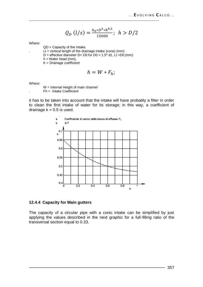
. . . E V O L V I N G C A L C O . . .

357

Where: QD = Capacity of the Intake. . Lt = vertical length of the drainage intake (cone) (mm) D = effective diameter D= D0 for D0 > 1.5* d1, Lt >D0 (mm) h = Water head (mm), K = Drainage coefficient

Where: W = Internal Height of main channel . Fh = Intake Coefficient

it has to be taken into account that the intake will have probably a filter in order to clean the first intake of water for its storage; in this way, a coefficient of drainage k = 0.5 is used.

12.4.4 Capacity for Main gutters

The capacity of a circular pipe with a conic intake can be simplified by just applying the values described in the next graphic for a full-filling ratio of the transversal section equal to 0.33.

. . . E V O L V I N G C A L C O . . .

358

Illustration 236 Wyly-Eaton hydraulic capacity calculation (Extracted from UNI-12056)

12.4.5 Results

Main gutters design Sheet

. . . E V O L V I N G C A L C O . . .

359

Gutters of the main Channels design Sheet

12.5 STORAGE TANK DESIGN 12.5.1 Monthly water catching

The expected monthly water catching rate is calculated according to the next equation:

. . . E V O L V I N G C A L C O . . .

360

Where: P = Average monthly rainfall (mm/month) A = Catchment area (m2) r = Rainoff coefficient n = system efficiency

Equation 24 Expected monthly water catching rate equation

For calculation purposes, it is considered an 85% of efficiency of the system, where 5 % of the water recollected is lost in the first flush and 15% for assumed evaporation rate. The runoff coefficient depends on the capacity of a surface to recollect water, taking into account the possible absorption and roughness properties that affect the final catchment of water.

Table 55 Rainoff coefficients (Extracted from H. Waterfall)

139

139

WATERFALL PATRICIA harvesting rainwater for landscape use. 2006. P 20

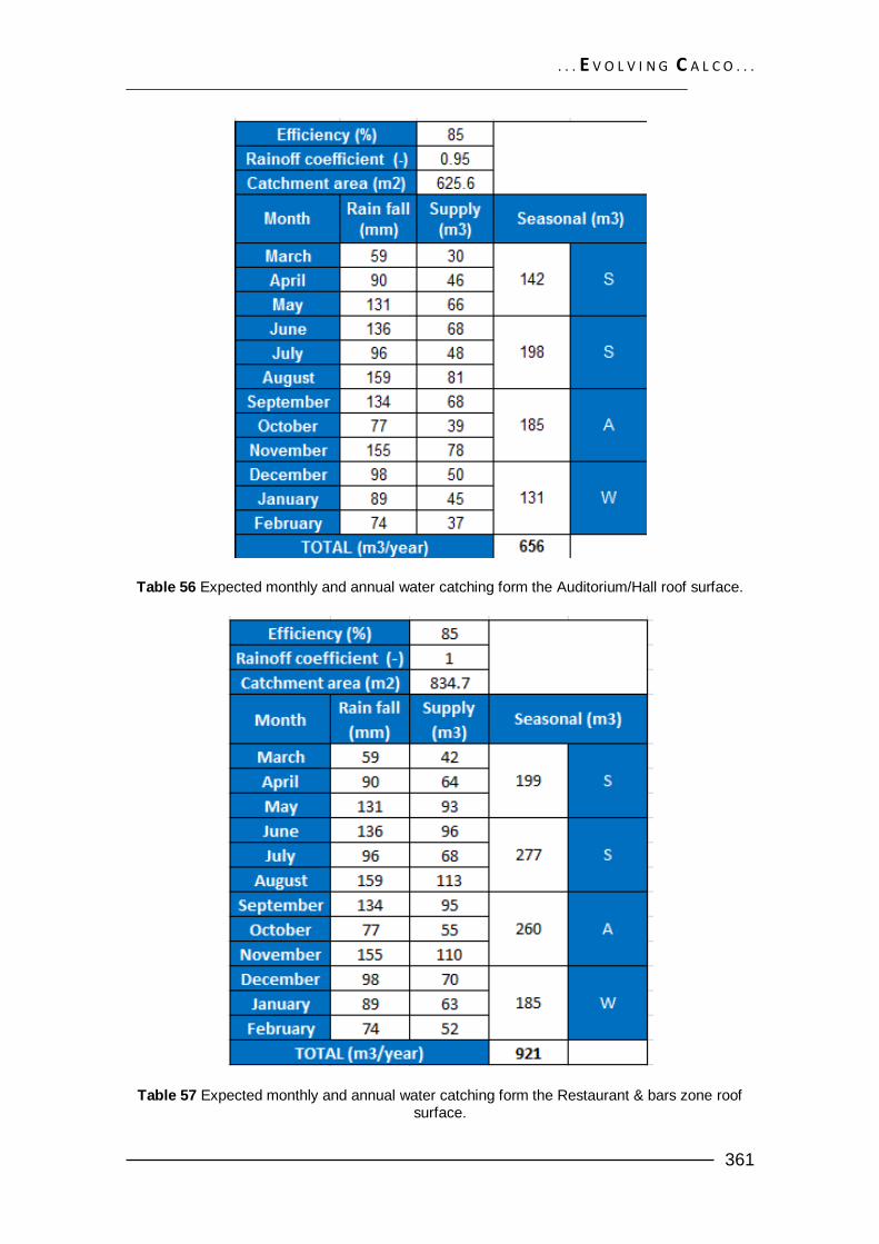
. . . E V O L V I N G C A L C O . . .

361

Table 56 Expected monthly and annual water catching form the Auditorium/Hall roof surface.

Table 57 Expected monthly and annual water catching form the Restaurant & bars zone roof surface.

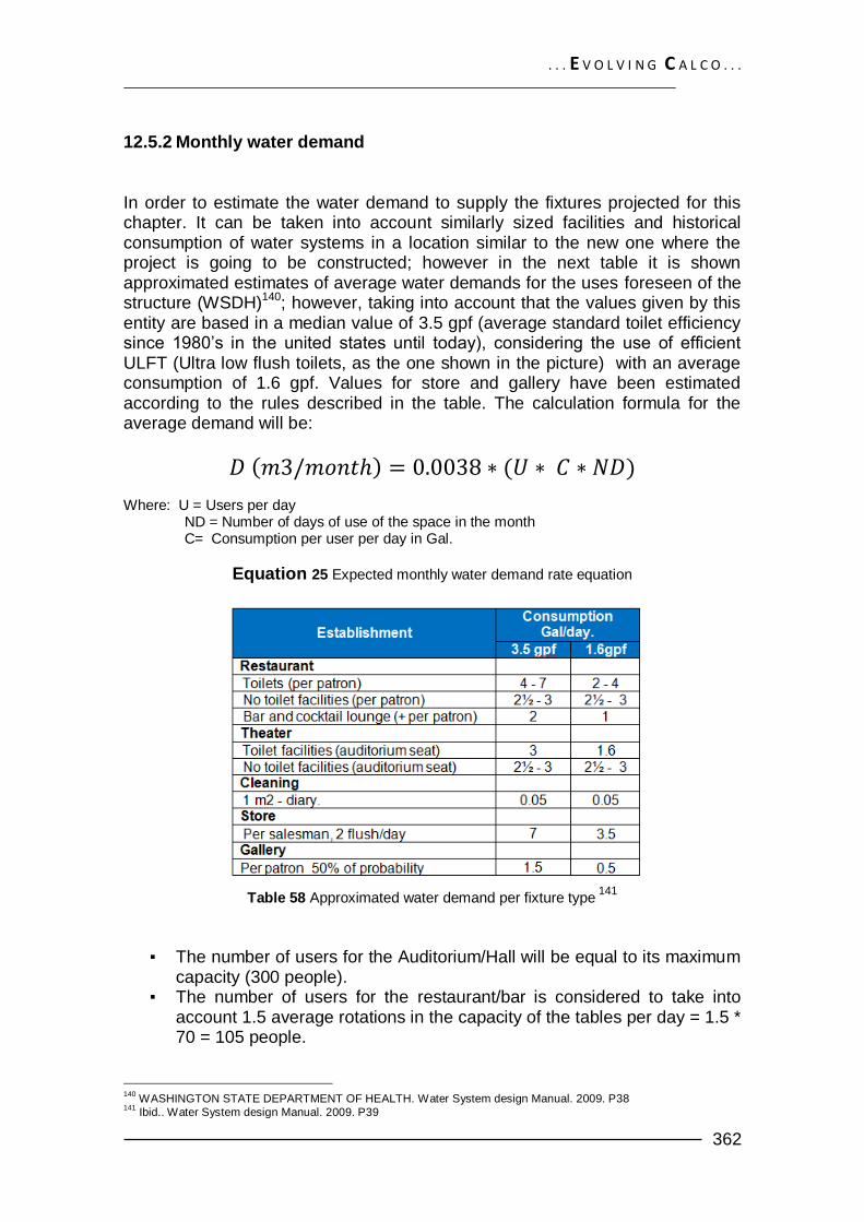
. . . E V O L V I N G C A L C O . . .

362

12.5.2 Monthly water demand

In order to estimate the water demand to supply the fixtures projected for this chapter. It can be taken into account similarly sized facilities and historical consumption of water systems in a location similar to the new one where the project is going to be constructed; however in the next table it is shown approximated estimates of average water demands for the uses foreseen of the structure (WSDH)140; however, taking into account that the values given by this entity are based in a median value of 3.5 gpf (average standard toilet efficiency since 1980’s in the united states until today), considering the use of efficient ULFT (Ultra low flush toilets, as the one shown in the picture) with an average consumption of 1.6 gpf. Values for store and gallery have been estimated according to the rules described in the table. The calculation formula for the average demand will be:

Where: U = Users per day ND = Number of days of use of the space in the month C= Consumption per user per day in Gal.

Equation 25 Expected monthly water demand rate equation

Table 58 Approximated water demand per fixture type

141

▪ The number of users for the Auditorium/Hall will be equal to its maximum

capacity (300 people). ▪ The number of users for the restaurant/bar is considered to take into

account 1.5 average rotations in the capacity of the tables per day = 1.5 * 70 = 105 people.

140

WASHINGTON STATE DEPARTMENT OF HEALTH. Water System design Manual. 2009. P38 141

Ibid.. Water System design Manual. 2009. P39

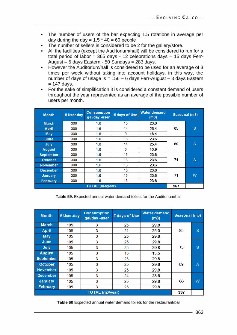
. . . E V O L V I N G C A L C O . . .

363

▪ The number of users of the bar expecting 1.5 rotations in average per day during the day = 1.5 * 40 = 60 people

▪ The number of sellers is considered to be 2 for the gallery/store. ▪ All the facilities (except the Auditorium/hall) will be considered to run for a

total period of labor = 365 days - 12 celebrations days – 15 days Ferr-August – 5 days Eastern - 50 Sundays = 283 days.

▪ However the Auditorium/hall is considered to be used for an average of 3 times per week without taking into account holidays, in this way, the number of days of usage is = 156 – 6 days Ferr-August – 3 days Eastern = 147 days.

▪ For the sake of simplification it is considered a constant demand of users throughout the year represented as an average of the possible number of users per month.

Table 59. Expected annual water demand toilets for the Auditorium/hall

Table 60 Expected annual water demand toilets for the restaurant/bar

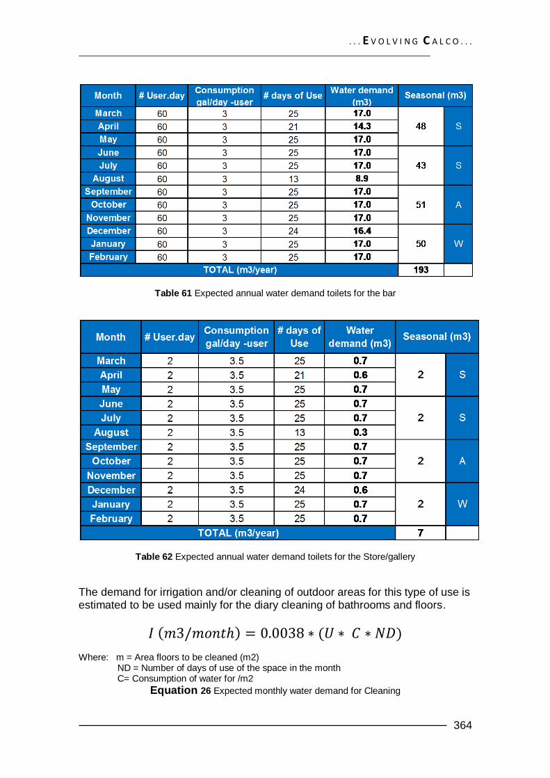
. . . E V O L V I N G C A L C O . . .

364

Table 61 Expected annual water demand toilets for the bar

Table 62 Expected annual water demand toilets for the Store/gallery

The demand for irrigation and/or cleaning of outdoor areas for this type of use is estimated to be used mainly for the diary cleaning of bathrooms and floors.

Where: m = Area floors to be cleaned (m2) ND = Number of days of use of the space in the month C= Consumption of water for /m2

Equation 26 Expected monthly water demand for Cleaning

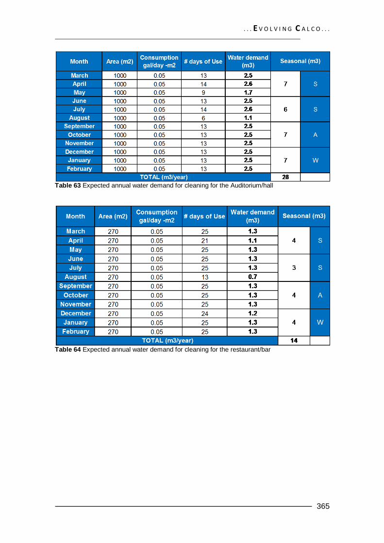
. . . E V O L V I N G C A L C O . . .

365

Table 63 Expected annual water demand for cleaning for the Auditorium/hall

Table 64 Expected annual water demand for cleaning for the restaurant/bar

. . . E V O L V I N G C A L C O . . .

366

Table 65 Expected annual water demand for cleaning for the bar and store/gallery (same area)

According to the expected supply of water from the recollection system, and the expected demand, it has been decided to satisfy 100% of the total demand due to the low needs of irrigation and toilets fixtures water demands 12.5.3 Storage capacity

For this purpose, the methodology suggested by the Texas water development board called the ―water balance method” consists on starting the calculation with an assumed volume of water already in the tanks, the volume captured each month is added to the previous balance and the demand is subtracted. The initial volume of water in the tanks would be provided by hauling or capturing water prior to withdrawing water from the system. The efficiency of the storage system will be assessed according to the final capacity given by the tank according to the total potential capacity given by a full storage system. Due to the values and demands obtained from the studies done before, it is decided to dimension a tank working at full storage capacity all the time.

Table 66 Calculation of storage needed for Auditorium/hall

. . . E V O L V I N G C A L C O . . .

367

The storage capacity is finally given in order to satisfy the total demand per month without incurring in high costs (due to storage capacity) or too low, but a high quantity of water wasted. For this aim, it has been decided to work with a efficiency of the water storage system close to the 40%, respect to the availability of water and the real storage.

Table 67. Calculation of storage needed for the restaurant/bars zone

In order to check the feasibility of the systems under dry conditions, it is assessed the capability of the storage tanks to not run out of water after a 21-days (3 weeks) dry period, which can occur usually in the month with less precipitation rate (March).

Table 68 Verification dry period capacity for Auditorium/Hall storage tank

. . . E V O L V I N G C A L C O . . .

368

Table 69 Verification dry period capacity for Restaurant/bar zone storage tank

12.5.4 Results: As a result of the analysis, there are considered:

▪ 2 storage tanks of a capacity equal to 9000 l/each and one of a capacity equal to 3000 lt to supply the Auditorium/hall system.

▪ On the other hand, for the Restaurant/bar zone, there are considered 5

storage tanks with a capacity of 9000 l/each + one with a capacity of 4500 l.

▪ The tanks must be located at a height (Base level) at least equal to + 2

m, in order to satisfy a minimum pressure in the appliances of around 20 kPa, when a low pressure valve is applied, or 50 kPa for other type and in order to satisfy better functioning of the fixture.

. . . E V O L V I N G C A L C O . . .

369

13 NET ZERO FOOT PRINT STANDARD

In order to achieve a Net zero foot print standard it is hereafter assessed the capacity of the system to produce or purchase renewable energy.

Illustration 237 NZEB Classification guide (Extracted from U.S Energy department) 142

142 Torcellini, Paul. Pless, Shanti. – U.S Department of Energy. Net Zero Energy Buildings: A Classification System

Based on Renewable Energy Supply Option. Pag 13. 2010.

. . . E V O L V I N G C A L C O . . .

370

1. Does the building have an annual Net zero balance for any of the NSEB definitions. ( Site, Source, Cost).

R: Yes!!, by sizing the photovoltaic system to supply the electric demand needed to run completely the building, the system would be able to generate and export to the grid as much energy as it is generated, even if the electrical energy storage is not enough on the site. A Net SITE zero balance can be achieved. 2. Does the building have Fossil-fuel powered generation equipment, and is

any of this energy exported to the grid part of the NZEB energy balance. R: No!!, al the systems that generate energy in the building does not operate with fossil fuels or another non-renewable type of combustible.

3. If the renewable sources required for NZEB status are sold as part of the

renewable energy system, are those credits purchased back? R: Yes! As a matter of fact, in case that the the electrical power would not be able to supply all the demand due to constant changing environmental conditions or unexpected energy consumptions, the system backup will rely on the idea of importing off-site electrical energy, which can be produced from hydroelectric available in the zone of the project. 4. Is any of the Renewable energy required for NSEB status purchased

from off-site sources?

R: Yes, as it was explained above. 5. Is capital equipment located on-site to convert all Renewable energy to a

useful form for the building?

R: Yes, it can be seen that all the systems designed into the building are powered by electric energy which are able to generate heat and cooling energy, operate ventilation systems, generate light, and other more uses. As a result the building can be categorized as:

NZEB: C

. . . E V O L V I N G C A L C O . . .

371

CONCLUSIONS By leaving behind the almost unified typological and historical references to Calco’s past, the project is seeking a contemporary authentic expression of Calco’s current and future ambitions, adding a new layer to Calco’s future. By the same token, leveled open spaces and green areas explore a new balance between urbanism and landscape. The subordination of ground and landscape by buildings has been reversed to offer a unique symbiotic experience. The building relates to the surroundings in scale, proportion and in the way it adds to the established rhythm of leveling masses along the back path. Yet, our aim is to create some kind of contrast, to express characteristic clarity, but most importantly to highlight the beauty of the surroundings. On aim achieved is also the use small means to create an array of different spatial experiences in this small project. TECHNOLOGICAL DESIGN The inclusion of renewable energy strategies such as small hydropower plants constitutes from the projection point of view, a profitable opportunity for the city of Calco which according to the data obtained, it could generate up to 8% of the total electrical consumption of the population with a payback time of 7 to 10 years of the infrastructure investment. On the other hand, it has to be underlined that the system configuration presented in the present project has attained the requirements of a net zero foot print building, acquiring a classification C. Achievement of 0.00 CO2 emissions for both heating and cooling systems by using renewable energy supply (PV panels and ground heat pumping), and a combination of energy saving strategies in matter of thermal behavior of the building and ventilation. The use of ETFE foils with integrated shading system connected to the building heating-cooling system constitutes a technical approach that can control the amount of radiation entering into the building, and, thus, reduce the cooling and heating demands throughout the whole year of operation. Characteristics considered in the building envelope components such as low thermal coefficients, but also the strategies considered in terms of solar orientation, operable glazed transition spaces and hybrid ventilation, have resulted into the reduction of the expected heating and cooling consumption of the building, (compared to traditional materials and heating/cooling systems) in a percentage of 60%

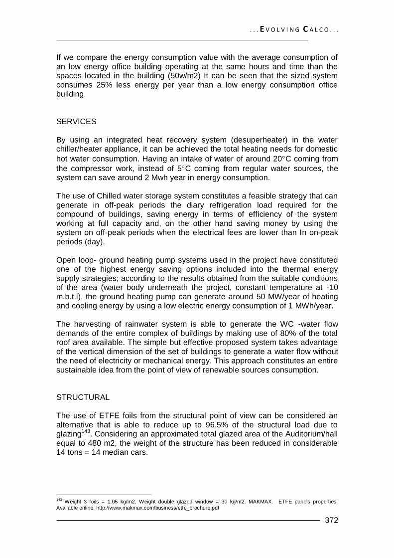
. . . E V O L V I N G C A L C O . . .

372

If we compare the energy consumption value with the average consumption of an low energy office building operating at the same hours and time than the spaces located in the building (50w/m2) It can be seen that the sized system consumes 25% less energy per year than a low energy consumption office building. SERVICES By using an integrated heat recovery system (desuperheater) in the water chiller/heater appliance, it can be achieved the total heating needs for domestic

hot water consumption. Having an intake of water of around 20C coming from

the compressor work, instead of 5C coming from regular water sources, the system can save around 2 Mwh year in energy consumption. The use of Chilled water storage system constitutes a feasible strategy that can generate in off-peak periods the diary refrigeration load required for the compound of buildings, saving energy in terms of efficiency of the system working at full capacity and, on the other hand saving money by using the system on off-peak periods when the electrical fees are lower than In on-peak periods (day). Open loop- ground heating pump systems used in the project have constituted one of the highest energy saving options included into the thermal energy supply strategies; according to the results obtained from the suitable conditions of the area (water body underneath the project, constant temperature at -10 m.b.t.l), the ground heating pump can generate around 50 MW/year of heating and cooling energy by using a low electric energy consumption of 1 MWh/year. The harvesting of rainwater system is able to generate the WC -water flow demands of the entire complex of buildings by making use of 80% of the total roof area available. The simple but effective proposed system takes advantage of the vertical dimension of the set of buildings to generate a water flow without the need of electricity or mechanical energy. This approach constitutes an entire sustainable idea from the point of view of renewable sources consumption. STRUCTURAL The use of ETFE foils from the structural point of view can be considered an alternative that is able to reduce up to 96.5% of the structural load due to glazing143. Considering an approximated total glazed area of the Auditorium/hall equal to 480 m2, the weight of the structure has been reduced in considerable 14 tons = 14 median cars.

143

Weight 3 foils = 1.05 kg/m2, Weight double glazed window = 30 kg/m2. MAKMAX. ETFE panels properties.

Available online. http://www.makmax.com/business/etfe_brochure.pdf

. . . E V O L V I N G C A L C O . . .

373

. . . E V O L V I N G C A L C O . . .

374

BIBLIOGRAPHY Books:

▪ AMERICAN STEEL JOIST INSTITUTE. Steel joists and joist girders: 5th

edition: VULCRAFT, Illinois – U.S.A. 2001. 130 p.

▪ ARCHITEN LANDRELL. ETFE foil: A guide to design. Chepstow – U.K. 2011. 14 P.

▪ AUSTRALIAN GOVERNMENT- National water commission. Rain water tank design and installation Hand-book. Australia. 2008. 21, 47 P.

▪ BARRON, Michael. Auditorium acoustics and Architectural design. 2d

Edition: SPON PRESS, New York – U.S.A. 2009. 249 P.

▪ CARRION Antoni. Diseño acústico de espacios architectonicos. 1st Edition: Universidad Politécnica de Catalunya, Barcelona – España, 1998. 137, 198-201, 209 P.

▪ GREENO, Roger; HALL, Fred. Building services handbook. 4th Edition:

ELSEVIER, Oxford – England, 2007.159 p.

▪ JACOBS, J. Death and Life of Great American Cities. Modern Library Edition, NewYork – U.S.A. 466 p.

▪ LYNCH, K., The Image of the City. Cambridge MA: The MIT Press: 2nd

edition. London-England. 1960. 194 p.

▪ ____________Good city form. Cambridge MA: The MIT Press: London-England. 1981. 194 p.

▪ MCQUAY International. Geothermal Heat pump design manual.

Application guide AG 31 -008. Appendix 1: Ground temperatures. Heating and cooling with a heat pump. Minnesota -U.S.A. 2011. 38 P.

▪ MINISTERIO DELLO SVILUPPO ECONOMICO. Decreto Legislativo 3

marzo 2011 N28. sulla promozione dell’uso dell’energia da fonti rinnovabili. Italia. 2011.

▪ MOSLEY Bill et al. Reinforced Concrete design to Eurocode 2. 6th

edition: Palgrave Macmillan, London – England, 2007. 420 p.

▪ PROVINCIA DI LECCO. Piano Energetico Territoriale Provinciale (PETP): Vol 2 Scenari, Obiettivi e Strumenti da Attuazione. Lecco - Italia. 2009. 4-44,120-121 P.

▪ SHAFTOE, Henry. Convivial urban spaces: creating effective public;

Sterling : Earthscan, London – England. 2008. 154 p.

. . . E V O L V I N G C A L C O . . .

375

▪ STRUCTURAL BUILDING COMPONENT ASSOCIATION. Guide for

good practice for specifying & applying loads to structural building components. Version 1.03. 2009. 212 p.

▪ TEXAS WATER DEVELOPMENT BOARD. The Texas Manual on

Rainwater harvesting. 3rd Edition: Austin – Texas, 2005. 32 p.

▪ THE CABELL BRAN CENTER Virginia Rainwater tank design and installation handbook. Salem – U.S.A. 2007. 33 P.

▪ THE INSTITUTION OF STRUCTURAL ENGINEERS, THE

INSTITUTION OF CIVIL ENGINEER. Manual for the design of steelwork building structures to Eurocode 3. 2nd edition: SETO, London - England, 2000. 138 p.

▪ THE STEEL CONSTRUCTION INSTITUTE. Section properties and

member resistances to Eurocode 3 (UB, UC and hollow sections): THE STEEL CONSTRUCTION INSTITUTE, London – England, 1997. 140 p.

▪ UNIRAC. Solar Mount. U.S.A. Des patent No. D496,248S. Code

compliant installation manual 227.3: UNIRAC, 2010. 26 p.

▪ UNITED STATES DEPARTMENT OF ENERGY. Consumer Guide, get your power from the sun. The National Renewable Energy Laboratory. Washington - U.S.A. 2010. 4-5 P.

▪ WASHINGTON STATE DEPARTMENT OF HEALTH. Water System

design Manual. Olympia – U.S.A. 2009. 37-39 P.

▪ WATERFALL, Patricia. Harvesting rainwater for Landscape use. 2nd Edition: COLLEGE OF AGRICULTIRE AND LIFE SCIENCES UNIVERSITY OF ARIZONA, Arizona – U.S.A. 2006. 20 P.

▪ WHYTE, H.W, the Social Life of Small Urban Spaces. New York: Project

for Public Spaces. Newyork- U.S.A. 1980. 128 p.

▪ YEANG, Ken. Eco-design: a manual for economical design. 2nd Edition: Wiley academy, London - England, 2006. 477 P.

Projects:

▪ PENATI Maurizio, TODESCHINI, Marialuisa. Indagine geologia tecnica ai sensi del D.M. 11.3 nel comune di Calco (Lc). 2003. 32 p.

▪ BRUI, Anne. Future proofing late postwar Neighbothoods: Urban

patterns for a socially sustainable Zevenkamp. Msc. In Architecture Thesis. TU Delft, faculty of architecture. Delft –Holland. 2010 249 p.

Standards:

. . . E V O L V I N G C A L C O . . .

376

▪ ENTE NAZIONALE ITALIANO DI UNIFICAZIONE. UNI EN ISO 10077-

1:2007 Prestazione termica di finestre, porte e chiusure oscuranti - Calcolo della trasmittanza termica - Parte 1: Generalità (EN 1994-03-31)

▪ __________________________________________. UNI 10351:1994

Materiali da costruzione. Conduttività termica e permeabilità al vapore. (EN 1994-03-31)

▪ EUROPEAN COMETEE FOR STANDARDIZATION. EUROCODE 2:

Design of concrete structures – Part 1: General rules and rules for buildings. Brussels, 2002. 226 p. (EN 1992-1-1)

▪ ______. EUROCODE 2: Design of concrete structures – Part 1.1:

General rules and rules for buildings. Brussels, 2004. 225 p. (EN 1992-1-1)


General actions – Snow load. Brussels, 2003. 56 p. (EN 1992-1-3)

▪ ______. EUROCODE 2: Design of concrete structures – Part 1.4: Lightweight aggregate concrete with closed structure. Brussels, 1996. 26 p. (EN 1996-1-4)


General rules - Plain concrete structures. Brussels, 1994. 24 p. (EN 1996-1-6)

▪ ______. EUROCODE 3: Design of steel structures – Part 1.1: General

structural rules. Brussels, 2001. 61 p. (EN 1993-1-1) ▪ ______. EUROCODE 8: Design of structures for earthquake resistance –

Part 1: General rules, seismic actions and rules for buildings. Brussels, 2003. 61 p. (EN 1998-1-1)

Articles:

▪ ACAA U.S.A. Advancing the management and use of coal combustion products. ECOBA 2006 CCP production & survey Europe. [on-line]. U.S.A: ACCA, 2011. [Reviewed on the 06 Jun. 2011]. Available at: http://www.acaa-usa.org/associations/8003/files/ECOBA_Stat_2006_ EU15.pdf.

▪ _____. Sustainable construction with coal combustion products. ECOBA

2006 CCP production & survey Europe. [on-line]. U.S.A: ACCA, 2011. [Reviewed on the 06 Jun. 2011]. Available at: http://www.acaa-usa.org/associations/8003/files/Sustainability_Construction_w_CCPs%28 Consolidated%29.pdf.

. . . E V O L V I N G C A L C O . . .

377

▪ BRADFORD WHITE. Sizing Commercial/Food services Heat water tanks [on-line]. U.S.A. [Reviewed on the 28 Jul. 2011] http://rightspec.bradfordwhite.com/ Sizing/FoodService.aspx

▪ BUBBLEDECK. The biaxial Hollow deck - design guide. [on-line].

England: BUBBLEDECK, 2011. [Reviewed on the 18 Aug. 2011]. Available at: http://www.bubbledeck.com/download/BD _INT_DesignGuide.pdf.

▪ CANOSOLAIR. Site orientation scheme [on-line]. U.S.A. [Reviewed on

the 14 Jul. 2011] Available at: http://www.cansolair. com/ features.php.

▪ CENTER FOR CIVIL ENGINEERING RESEARCH CODES. Bubble deck floors, supplementary regulations to NEN 6720:1995. CUR, Leiden - the Netherlands. 2003. CUR R-86.

▪ COBIAX. Benefits of the Cobiax slab technology. [on-line]. Switzeland:

COBIAX, 2011. [Reviewed on the 25 JuL. 2011]. Available at: http://www.cobiax.ch/downloads/english/Cobiax_Brochure_ E_2010.pdf.

▪ DEGELMAN, Legel et allTthe framework of an optimization model for the

thermal design of building envelopes. Proceedings of the Ninth Symposium on Improving Building Systems in Hot and Humid Climate. Arlington texas.1994 p 254.

▪ GREENSPEC., Photo Voltaic (PV) Cells. [on-line]. Italy. [Reviewed on

the 21 Jul. 2011] Available at: http://greenspec.co.uk/pv-cells.php

▪ __________. Ground source heating pumps. [on-line]. Italy. [Reviewed on the 19 Jul. 2011] Available at: http://greenspec.co.uk /ground-source-heat-pumps.php

▪ __________. Passive solar design: sun spaces. [on-line]. Italy.

[Reviewed on the 21 Jul. 2011] Available at: http://greenspec.co.uk /passive-solar-sunspaces.php

▪ __________. Passive solar design: sitting and orientation. [on-line]. Italy.

[Reviewed on the 22 Jul. 2011] Available at: http://greenspec.co.uk/solar-siting-orientation.php

▪ H.M, RAMOS Et al. Clean power in water supply systems as a

sustainable solution: from planning to practical implementation. Magazine Water Science & Technology: Water Supply—WSTWS. E.U. 2010. Volume 10, Number 1, 47 P.

▪ ISIS Arturo Malignani Udine. Alternative power sources at different

latitudes in Europe [on-line]. Italy. [Reviewed on the 14 Jul. 2011] Available at: http://www.malignani.ud.it/webenis/northwind-southsun/power/Biomass.htm


. . . E V O L V I N G C A L C O . . .

378

▪ INSTITUTO NAZIONALE DI GEOFISICA E VULCANOLOGIA. Zone sismiche regionali Italia. [on-line]. Italia: INDGEV, 201. [Reviewed on the 25 Jul. 2011]. Available at: http://zonesismiche.mi.ingv.it/

▪ ISTITUTO NAZIONALE DI STATISTICA. Demographic Balance for the

year 2010 and resident population on 31th December, Calco. [on-line]. Italy. [Reviewed on the 29 May. 2011] Available at: http://demo.istat.it/bil2010/index02_e.html

▪ JOINT RESEARCH CENTRE. Photovoltaic geographical information

system, interactive maps. [on-line]. E.U. [Reviewed on the 31 Jul. 2011] Available at: http://re.jrc.ec. europa.eu/pvgis/ apps4/ pvest.php

▪ MAKMAX. [on-line]. ETFE Panels solutions. Japan: MAKMAX, 2011.

[Reviewed on the 8 Aug. 2011]. Available at: http://www.makmax.com/business /etfe_brochure.pdf.

▪ MY ENERGY, Calcolo simulazione impianto fotovoltaici per casa di

famiglia, media provincial di Lecco. [on-line]. Italy. [Reviewed on the 21 Jul. 2011] Available at: http://www.myenergy.it/conto-energia/simula-impianto/simula-impianto.aspx

▪ NATIONAL READY MIXED CONCRETE ASSOCIATION. NRCMA.

Concrete in practice [on-line]. U.S.A: NRMCA, 2011. [Reviewed on the 30 Jul. 2011]. Available at: http://www.nrmca.org/ aboutconcrete/cips/33p.pdf.

▪ NATURAL RESOURCES OF CANADA. Heating and cooling with a heat

pump. [on-line]. Canada. [Reviewed on the 06 Ago. 2011] http://oee.nrcan.gc.ca/publications/infosource/pub/home/Heating_and_Cooling _with_a_Heat_Pump_Section4.cfm

▪ NOAA satellite and information site. HDD locations United States

Department of Commerce. [on-line]. U.S.A. [Reviewed on the 27 Jul. 2011]. Available at. http://www.ncdc.noaa.gov/oa/climate/online/ccd/nrmhdd.txt

▪ REUK Uk. Ligh tubes for interior lighting article 2007 [on-line]. U.S.A.

[Reviewed on the 26 May. 2011]. Available at: http://www.reuk.co.uk/Light-Tubes-for-Interior-Lighting.htm

▪ RICERCA SISTEMA ENERGETICFO. Atlante Eolico Italiano. 2011. [on-

line]. ITALY. [Reviewed on the 23 of May. 2011]. Available at: http://atlanteeolico.rse-web.it/viewer.htm

▪ SOLATUBE. Side lighting vs. Top lighting [on-line]. U.S.A. [Reviewed on

the 25 May. 2011].http://www.solatube.com/commercial/daylighting/top-lighting-vs-side-lighting.php

http://demo.istat.it/bil2010/index02_e.html



http://www.ncdc.noaa.gov/oa/climate/online/ccd/nrmhdd.txt


http://www.solatube.com/

. . . E V O L V I N G C A L C O . . .

379

▪ SUSTAINABLE SOURCES. Flyash concrete. [on-line]. U.S.A: SOUSTAINABLE SOURCES, 2011. [Reviewed on the 10 Jun. 2011]. Available at: http://flyash.sustainablesource s.com/#USE.

▪ THE STRUCTURAL BUILDING COMPONENTS INDUSTRY Cold-

formed steel building development safety information: edition 2008 COLD FORMED STEEL COUNCIL, 2008, 85 P.

▪ UNITED STATES DEPARTMENT OF ENERGY. Types of Geothermal

Heat Pump Systems. [on-line]. U.S.A. [Reviewed on the 03 Ago. 2011]. Available at: http://www.energysavers.gov/your_home/space_heating_cooling/index.cfm/mytopic=12650.2011

▪ ________________________________________. Types of Hydropower

Plants. [on-line]. U.S.A. [Reviewed on the 02 Ago. 2011]. Available at: http://www1.eere.energy.gov/windandhydro/hydro_plant_types.html. 2011

▪ ________________________________________. Sizing Storage and

Heat Pump (with Tank) Water Heaters. on-line]. U.S.A. [Reviewed on the 02 Ago. 2011]. Available at: http://www.energysavers.gov/your_home/ water_heating/index.cfm/mytopic=12990

▪ UNIVERSITY OF OREGON. Solar radiation monitoring laboratory. [on-

line]. U.S.A. [Reviewed on the 25 Jul. 2011]. Available at: http://solardat.uoregon.edu/SunChartProgram.html

▪ VECTORFOILTEC. Texlon technical specifications. [on-line]. U.S.A.

[Reviewed on the 02 May. 2011]. Available at: http://www.vector-foiltec.com/cms /gb/ technical/ randd.php

▪ _______________. Variable skins. [on-line]. U.S.A. [Reviewed on the 03

May. 2011]. Available at: http://www.vector-foiltec.com/cms/gb/technical /variableskins.php

▪ _______________. Ventilation systems. [on-line]. U.S.A. [Reviewed on

the 02 May. 2011]. Available at: http://www.vector-foiltec.com/cms/gb /technical/ ventilation.php

▪ WIENER, Ethan. Acoustic treatment and design for listening rooms and

recording studios. [on-line]. U.S.A. [Reviewed on the 10 Ago. 2011]. http://www.ethanwiner.com/acoustics.html

▪ WEATHER UNDERGROUND. Historical data private meteorological

station No. I90580765. [on-line]. U.S.A. [Reviewed on the 30 Jul. 2011]. Available at: http://www.wunderground.com/weatherstation/WXDailyHistory.asp?ID= I90580765.




. . . E V O L V I N G C A L C O . . .

380

ACKNOWLEDGEMENT The authors express their more sincere thanks to the Architect & professor Massimo Tadi for his support and remarkable guidance throughout the development of this project. Special gratitude is presented to professors Danilo Palazzo, Gabriele Masera, Liberato Ferrara and Giuseppe Rapisarda for the help given by their immense knowledge and inspiration in the Urban, Technological, Structural and Building services’ design areas respectively. Acknowledgement is directed to the companies Vector Foiltec and Clima size for their interest and support on the project technologies employed. We also thank gratefully to our families and beloved friends for their unconditional love and support. Thank you all.

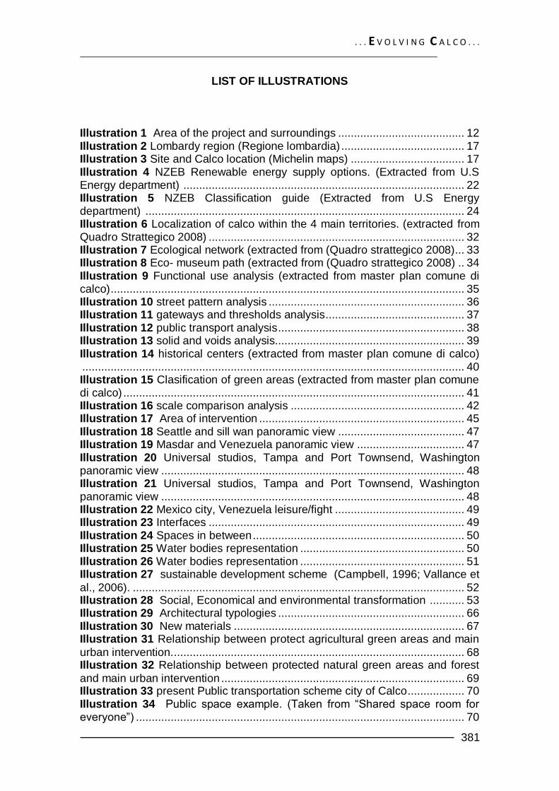
. . . E V O L V I N G C A L C O . . .

381

LIST OF ILLUSTRATIONS

Illustration 1 Area of the project and surroundings ........................................ 12

Illustration 2 Lombardy region (Regione lombardia) ....................................... 17 Illustration 3 Site and Calco location (Michelin maps) .................................... 17

Illustration 4 NZEB Renewable energy supply options. (Extracted from U.S Energy department) ......................................................................................... 22 Illustration 5 NZEB Classification guide (Extracted from U.S Energy department) ..................................................................................................... 24 Illustration 6 Localization of calco within the 4 main territories. (extracted from Quadro Strattegico 2008) ................................................................................. 32 Illustration 7 Ecological network (extracted from (Quadro strattegico 2008)... 33 Illustration 8 Eco- museum path (extracted from (Quadro strattegico 2008) .. 34

Illustration 9 Functional use analysis (extracted from master plan comune di calco) ................................................................................................................ 35 Illustration 10 street pattern analysis .............................................................. 36 Illustration 11 gateways and thresholds analysis ............................................ 37

Illustration 12 public transport analysis ........................................................... 38 Illustration 13 solid and voids analysis............................................................ 39

Illustration 14 historical centers (extracted from master plan comune di calco) ......................................................................................................................... 40 Illustration 15 Clasification of green areas (extracted from master plan comune di calco) ............................................................................................................ 41 Illustration 16 scale comparison analysis ....................................................... 42 Illustration 17 Area of intervention ................................................................. 45

Illustration 18 Seattle and sill wan panoramic view ........................................ 47 Illustration 19 Masdar and Venezuela panoramic view .................................. 47

Illustration 20 Universal studios, Tampa and Port Townsend, Washington panoramic view ................................................................................................ 48 Illustration 21 Universal studios, Tampa and Port Townsend, Washington panoramic view ................................................................................................ 48 Illustration 22 Mexico city, Venezuela leisure/fight ......................................... 49 Illustration 23 Interfaces ................................................................................. 49

Illustration 24 Spaces in between ................................................................... 50 Illustration 25 Water bodies representation .................................................... 50

Illustration 26 Water bodies representation .................................................... 51 Illustration 27 sustainable development scheme (Campbell, 1996; Vallance et

al., 2006). ......................................................................................................... 52 Illustration 28 Social, Economical and environmental transformation ........... 53 Illustration 29 Architectural typologies ........................................................... 66

Illustration 30 New materials ......................................................................... 67 Illustration 31 Relationship between protect agricultural green areas and main

urban intervention. ............................................................................................ 68 Illustration 32 Relationship between protected natural green areas and forest

and main urban intervention ............................................................................. 69 Illustration 33 present Public transportation scheme city of Calco .................. 70

Illustration 34 Public space example. (Taken from ―Shared space room for everyone‖) ........................................................................................................ 70

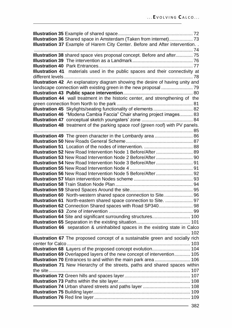
. . . E V O L V I N G C A L C O . . .

382

Illustration 35 Example of shared space ......................................................... 72

Illustration 36 Shared space in Amsterdam (Taken from internet) .................. 73 Illustration 37 Example of Harem City Center. Before and After intervention. .

......................................................................................................................... 74 Illustration 38 shared space vies proposal concept. Before and after............. 75

Illustration 39 The intervention as a Landmark .............................................. 76 Illustration 40 Park Entrances ........................................................................ 77

Illustration 41 materials used in the public spaces and their connectivity at different levels .................................................................................................. 78 Illustration 42 An explanatory diagram showing the desire of having unity and landscape connection with existing green in the new proposal ........................ 79 Illustration 43 Public space intervention ..................................................... 80 Illustration 44 wall treatment in the historic center, and strengthening of the

green connection from North to the park .......................................................... 81 Illustration 45 Skylights/seating functionality of elements .............................. 82

Illustration 46 ―Modena Cambia Faccia‖ Chair sharing project images.......... 83 Illustration 47 conceptual sketch youngsters’ zone ....................................... 84

Illustration 48 treatment of the parking space roof (green roof) with PV panels. ......................................................................................................................... 85 Illustration 49 The green character in the Lombardy area ............................. 86 Illustration 50 New Roads General Scheme ................................................... 87

Illustration 51 Location of the nodes of intervention. ..................................... 88 Illustration 52 New Road Intervention Node 1 Before/After ............................ 89

Illustration 53 New Road Intervention Node 2 Before/After ............................ 90 Illustration 54 New Road Intervention Node 3 Before/After ............................ 91

Illustration 55 New Road Intervention Node 4 ................................................ 91 Illustration 56 New Road Intervention Node 5 Before/After ............................ 92

Illustration 57 Main intervention Nodes scheme ............................................. 93 Illustration 58 Train Station Node Plan ........................................................... 94

Illustration 59 Shared Spaces Around the site ................................................ 95 Illustration 60 North-western shared space connection to Site. ..................... 96

Illustration 61 North-eastern shared space connection to Site. ..................... 97 Illustration 62 Connection Shared spaces with Road SP340 .......................... 98

Illustration 63 Zone of intervention ................................................................ 99 Illustration 64 Site and significant surrounding structures............................. 100

Illustration 65 Separation in the existing situation ......................................... 101 Illustration 66 separation & uninhabited spaces in the existing state in Calco

....................................................................................................................... 102 Illustration 67 The proposed concept of a sustainable green and socially rich

center for Calco .............................................................................................. 103 Illustration 68 Layers of the proposed concept evolution............................. 104 Illustration 69 Overlapped layers of the new concept of intervention ............ 105

Illustration 70 Entrances to and within the main park area ........................... 106 Illustration 71 New Hierarchy of the streets, paths and shared spaces within

the site ............................................................................................................ 107 Illustration 72 Green hills and spaces layer .................................................. 107

Illustration 73 Paths within the site layer....................................................... 108 Illustration 74 Urban shared streets and paths layer .................................... 108

Illustration 75 Building layer .......................................................................... 109 Illustration 76 Red line layer ......................................................................... 109

. . . E V O L V I N G C A L C O . . .

383

Illustration 77 conceptual final outcome of the new proposal ....................... 111

Illustration 78 The Urban Zone (Shared spaces) cutting through the site ..... 112 Illustration 79 The Park Zone within the site ................................................. 113

Illustration 80 The Mass Zone emerging from the site .................................. 114 Illustration 81 The three zones overlapped, showing the final result ............ 115

Illustration 82 Final layout proposal integrated within the context ................. 116 Illustration 83 Final layout proposal integrated within the context ................. 117

Illustration 84 Main zoning areas in relation with the site.............................. 118 Illustration 85 Detailed zoning of the intervention area ................................. 119

Illustration 86 Project’s View. ........................................................................ 119 Illustration 87 Accessibility diagram .............................................................. 121

Illustration 88 Study of the whole structure morphology ............................... 122 Illustration 89 Study of the blow up of all the masses design within the site . 122

Illustration 90 Study of the blow up of the main two buildings (MPH / Auditorium and the Restaurant, Bar and Gallery Zones) ................................ 123 Illustration 91 Study of the blow up of the main space in the project (MPH / Auditorium) ..................................................................................................... 123 Illustration 92 relation between the groundline, skyline and greenlines in various sections in the project ........................................................................ 124 Illustration 93 Final Proposed Layout ........................................................... 125 Illustration 94 Final Proposal Plan ................................................................ 126

Illustration 95 Horizontal Section Lines......................................................... 127 Illustration 96 Final Proposal South Elevation .............................................. 127

Illustration 97 Final Proposal Section AA01 .................................................. 127 Illustration 98 Final Proposal Section AA02 .................................................. 127

Illustration 99 Vertical Section Lines ............................................................ 128 Illustration 100 Final Proposal Section BB01 ............................................... 128

Illustration 101 Final Proposal Section BB02 / West Elevation 01 ............... 128 Illustration 102 Final Proposal Section BB03 ............................................... 128

Illustration 103 Final Proposal Section BB04 ............................................... 129 Illustration 104 Final Proposal Section BB05 / West Elevation 02 ............... 129

Illustration 105 Full San Vigilio Intervention Proposal .................................. 129 Illustration 106 Shot showing the relation between the project and the existing

context ............................................................................................................ 130 Illustration 107 View from the Church (Bird’s Eye) ....................................... 131

Illustration 108 View from the West end of the project, highlighting the visual relation between the back path and the church, as well as the functional relation with the rest of the project .............................................................................. 131 Illustration 109 Shot from the San Vigilio Church Entrance .......................... 133

Illustration 110 interconnection in accessibility and functional relations ....... 134 Illustration 111 back path and main entrances to the site ............................ 134 Illustration 112 relation between the children zone and the catering zone .. 135

Illustration 113 relation of the youngsters zone with the palazzo dello sport and the Auditorium Zone ....................................................................................... 136 Illustration 114 relation between the back path, bar and the palazzo .......... 136 Illustration 115 A view from the linear park (Facing North – San Vigilio on the

right) ............................................................................................................... 137 Illustration 116 A view from the linear park (Facing South – San Vigilio on the

left) ................................................................................................................. 137

. . . E V O L V I N G C A L C O . . .

384

Illustration 117 Green walls and Red Line treatment in the small historic center

street .............................................................................................................. 138 Illustration 118 abstraction of the prevailing materials in the existing situation

and the new proposal ..................................................................................... 139 Illustration 119 Interior shot of the Multi-purpose Auditorium/Hall Zone ....... 139

Illustration 120 Project expected ground stratigraphy (Extracted from PENATI) ....................................................................................................................... 144 Illustration 121 Comparison conventional system/hollow slab (Extracted from COBIAX)......................................................................................................... 147 Illustration 122 Maximum span according to open web steel joist classification (Extracted from VULCRAFT) .......................................................................... 148 Illustration 123 Open web steel joist conventional configuration (Extracted from VULCRAFT) ................................................................................................... 148 llustration 124 European snow map (Extracted from EUROCODE1-3) ........ 165 Illustration 125 Snow load at sea level for Alpide zone (Extracted from

EUROCODE1-3) ............................................................................................ 165

Illustration 126 partial safety factor at ultimate limit state, g and Q values. (Extracted from Mosley et al) .......................................................................... 171

Illustration 127 0, 1 and 2 values for different load combinations (Extracted from Mosley et al) ........................................................................................... 171 Illustration 128 Small Hydroelectric power scheme (extracted from US department of energy.) ................................................................................... 226 Illustration 129 Biomass power generation and coppicing schemes (extracted from ISIS) ....................................................................................................... 227 Illustration 130. Calco’s north-oriental forest and agricultural fields .............. 228 Illustration 131. Hybrid Solar photovoltaic energy power scheme (extracted

from US. Department of Energy) .................................................................... 229 Illustration 132. GSHP closed loop systems scheme (extracted from US

department of energy) .................................................................................... 230 Illustration 133. GSHP Open loop systems scheme (extracted from US

department of energy) .................................................................................... 230 Illustration 134. Passive-Gravity rainwater recollection system scheme

(extracted from AUSgov) ................................................................................ 232 Illustration 135 Active rainwater recollection system scheme (extracted from

AUSgov) ......................................................................................................... 232 Illustration 136 Sun tunnel scheme (extracted from SOLATUBE) ................ 233

Illustration 137. sun shading system system. Open and closed configuration (extracted from VECTORFOILTEC) ............................................................... 234 Illustration 138 Configuration of three foils with sun shading system foil (extracted from VECTORFOILTEC) ............................................................... 234 Illustration 139 Typical structural system and connections of the system (extracted from ARCHITEN) ........................................................................... 235 Illustration 140 Ventilation systems for ETFE pneumatic cushions (extracted from VECTORFOILTEC) ................................................................................ 235 Illustration 141. Buffer effect of sunspace, natural and mechanical ventilation advantages scheme. (extracted from GREENSPEC) ..................................... 236 Illustration 142 Building orientation scheme towards south. (Extracted from

CANOSOLAIR) ............................................................................................... 236

. . . E V O L V I N G C A L C O . . .

385

Illustration 143 Ceiling and wall convex and reflective surfaces (extracted from

CARRION) ...................................................................................................... 238 Illustration 144 Solutions to avoid echo (extracted from CARRION) ............ 239

Illustration 145 Slab SG-02 Condensation risk analysis ............................... 253 Illustration 146 Kitchen Bar – Viewer in the Middle and Standing – thermal

comfort analysis ............................................................................................. 256 Illustration 147 Graphical representation of the solar path in winter ............. 258

Illustration 148 Graphical Representation of the Solar Path in spring .......... 259 Illustration 149 Graphical Representation of the Solar Path in summer ....... 260

Illustration 150 Graphical Representation of the Solar Path in autumn ........ 261 Illustration 151 Graphical Representation of the average Temperature for the

city of Bergamo .............................................................................................. 263 Illustration 152Graphical Representation of the Relative Humidity for the city of

Bergamo ......................................................................................................... 263 Illustration 153 Graphical Representation of the average Cloud Cover for the

city of Milano .................................................................................................. 264 Illustration 154 Highlighted zone (Bar) in Case A ......................................... 266

Illustration 155 Daylight Factor in Plan (Bar) – Without Okalux or Shed...... 266 Illustration 156 Daylight Factor in Section (Bar) – Without Okalux or Shed .. 267

Illustration 157 Daylight Autonomy in Plan (Bar) – Without Okalux or Shed... 267 Illustration 158 Daylight Autonomy in Plan (Bar) – Without Okalux or Shed. 268

Illustration 159 Highlighted zone (Bar) in Case B ......................................... 268 Illustration 160 Daylight Factor in Plan (Bar) – With Okalux and Shed ......... 269

Illustration 161 Daylight Factor in Section (Bar) – With Okalux and Shed .... 269 Illustration 162 Daylight Autonomy in Plan (Bar) – With Okalux and Shed .. 270

Illustration 163 Daylight Autonomy in Section (Bar) – With Okalux and Shed ....................................................................................................................... 270 Illustration 164 Highlighted zone (Gallery/Store) in Case A .......................... 271 Illustration 165 Daylight Factor in Plan (Gallery/Store) – Without Okalux or

Shed ............................................................................................................... 272 Illustration 166 Daylight Factor in Section (Gallery/Store) – Without Okalux or

Shed ............................................................................................................... 272 Illustration 167 Daylight Autonomy in Plan (Gallery/Store) – Without Okalux or

Shed ............................................................................................................... 273 Illustration 168 Daylight Autonomy in Plan (Gallery/Store) – Without Okalux or

Shed ............................................................................................................... 273 Illustration 169 Highlighted zone (Gallery/Store) in Case B .......................... 274

Illustration 170 Daylight Factor in Plan (Gallery/Store) – With Okalux and Shed ............................................................................................................... 274 Illustration 171 Daylight Factor in Section (Gallery/Store) – With Okalux and Shed ............................................................................................................... 275 Illustration 172 Daylight Autonomy in Plan (Gallery/Store) – With Okalux and

Shed ............................................................................................................... 275 Illustration 173 Daylight Autonomy in Section (Gallery/Store) – With Okalux

and Shed ........................................................................................................ 276 Illustration 174 Highlighted zone (Restaurant) in Case A ............................. 277

Illustration 175 Highlighted zone (Restaurant) in Case B ............................. 277 Illustration 176 Daylight Factor in Plan (Restaurant) – Without Okalux or Shed

....................................................................................................................... 278

. . . E V O L V I N G C A L C O . . .

386

Illustration 177 Daylight Factor in Section (Restaurant) – Without Okalux or

Shed ............................................................................................................... 278 Illustration 178 Daylight Autonomy in Plan (Restaurant) – Without Okalux or

Shed ............................................................................................................... 279 Illustration 179 Daylight Autonomy in Plan (Restaurant) – Without Okalux or

Shed ............................................................................................................... 279 Illustration 180 Daylight Factor in Plan (Restaurant) – With Okalux and Shed

....................................................................................................................... 280 Illustration 181 Daylight Factor in Section (Restaurant) – With Okalux and

Shed ............................................................................................................... 280 Illustration 182 Daylight Autonomy in Plan (Restaurant) – With Okalux and

Shed ............................................................................................................... 281 Illustration 183 Daylight Autonomy in Section (Restaurant) – With Okalux and

Shed ............................................................................................................... 281 Illustration 184 Highlighted zone (Transitional zone) in Case A ................... 283

Illustration 185 Daylight Factor in Plan (T.Z.(A)) – With ETFE ..................... 283 Illustration 186 Daylight Factor in Section (T.Z.(A)) – With ETFE ................. 284

Illustration 187 Daylight Autonomy in Plan (T.Z.(A)) – With ETFE ............... 284 Illustration 188 Daylight Autonomy in Section (T.Z.(A)) – With ETFE .......... 285

Illustration 189 Highlighted zone (Transitional zone) in Case B ................... 285 Illustration 190 Daylight Factor in Plan (T.Z.(B)) – With ETFE .................... 286

Illustration 191 Daylight Factor in Section (T.Z.(B)) – With ETFE ................ 286 Illustration 192 Daylight Factor in Plan (T.Z.(B)) – With ETFE .................... 287

Illustration 193 Daylight Autonomy in Section (T.Z.(B)) – With ETFE .......... 287 Illustration 194 Daylight Factor in Plan (Exhibition) ...................................... 288

Illustration 195 Daylight Factor in Section (Exhibition).................................. 288 Illustration 196 Daylight Factor in Plan (Exhibition) ..................................... 289

Illustration 197 Daylight Autonomy in Section (Exhibition)........................... 289 Illustration 198 Total Monthly Solar Exposure – SOUTH ELEV – Without

Okalux or Shed ............................................................................................... 292 Illustration 199 Total Monthly Solar Exposure – SOUTH ELEV – With Okalux

....................................................................................................................... 292 Illustration 200 Total Monthly Solar Exposure – SOUTH ELEV – With

Okalux+Shed .................................................................................................. 293 Illustration 201 Total Monthly Solar Exposure – WEST ELEV – Without Shed

....................................................................................................................... 294 Illustration 202 Total Monthly Solar Exposure – WEST ELEV – With Shed . 295

Illustration 203 Total Monthly Solar Exposure – EAST ELEV – Without Shed ....................................................................................................................... 296 Illustration 204 Total Monthly Solar Exposure – EAST ELEV – With Okalux 296 Illustration 205 Total Monthly Solar Exposure – EAST ELEV – With Okalux + Shed ............................................................................................................... 297 Illustration 206 Total monthly Heating/Cooling Loads Auditorium Hall building (CASE A) ........................................................................................................ 302 Illustration 207 Total monthly Heating/Cooling Loads Auditorium Hall building (CASE B) ........................................................................................................ 306 Illustration 208 Total monthly Heating/Cooling Loads Restaurant/bar building (CASE A) ........................................................................................................ 307 Illustration 209 Total monthly Heating/Cooling Loads Restaurant/bar building (CASE B) ........................................................................................................ 311

. . . E V O L V I N G C A L C O . . .

387

Illustration 210 Zone 1 and 2 summer air conditioning scheme .................... 314

Illustration 211 Zone 1 and 2 winter air conditioning scheme ....................... 314 Illustration 212 Zone 3 and 4 winter air conditioning scheme ....................... 315

Illustration 213 Zone 3 and 4 summer air conditioning scheme .................... 316 Illustration 214 Zone 5 winter air conditioning scheme ................................. 317

Illustration 215 Zone 5 summer air conditioning scheme.............................. 317 Illustration 216. Winter Heating energy system supply ................................. 327

Illustration 217. Summer cooling energy system supply ............................... 328 Illustration 218. Winter water heating source plan ........................................ 329

Illustration 219. Summer water heating source plan ..................................... 329 Illustration 220 Winter GHP internal Heating cycle. ...................................... 330

Illustration 221 Summer GHP internal Cooling cycle. ................................... 330 Illustration 222 Bradford white calculation form ............................................ 334

Illustration 223 Bradford white calculation form without desuperheater ........ 336 Illustration 224 Photovoltaic system scheme. ............................................... 338

Illustration 225 Auditorium/hall water catching system - gutters and channels scheme ........................................................................................................... 348 Illustration 226 Restaurant/bar water catching system - gutters and channels scheme ........................................................................................................... 348 Illustration 227 Restaurant/bar storage and supply scheme ......................... 349 Illustration 228 Auditorium/hall storage and supply scheme ......................... 350

Illustration 229 channels distribution in the building (roof - plan view) ......... 350 Illustration 230 Risk coefficients k. (Extracted from UNI-12056) ................... 352

Illustration 231 Height relation coefficient Fd. (Extracted from UNI-12056) .. 353 Illustration 232 Shape relation coefficient Fd.. (Extracted from UNI-12056) . 353

Illustration 233 Discharge coefficient for long channels (Extracted from UNI-12056) ............................................................................................................ 354 Illustration 234 Main Gutters distribution in the building (roof - plan view) .... 356 Illustration 235 Gutters of main channel distribution in the building (roof - plan

view) ............................................................................................................... 356 Illustration 236 Wyly-Eaton hydraulic capacity calculation (Extracted from UNI-

12056) ............................................................................................................ 358 Illustration 237 NZEB Classification guide (Extracted from U.S Energy

department) ................................................................................................... 369

LIST OF GRAPHICS Graphic 1 Population compared to the main cities of the Brianza Lechesse region and Lecco (Istat 2010) ........................................................................... 16 Graphic 2 growing rate compared to the main cities of the Brianza Lechesse region and Lecco (Istat 2010) ........................................................................... 16 Graphic 3 Buildings structural distribution and uses ...................................... 142 Graphic 4 Analytical model Restaurant/bar in SAP 2000. ............................. 149

Graphic 5 Analytical model Auditorium/hall in SAP 2000. ............................. 152 Graphic 6 Restaurant/bar beams loaded by the Staircase model G2 first

loading (kN/m2) and reactions (kN/m) ............................................................ 155 Graphic 7 Restaurant/bar ceiling slab G2 loading (kN/m2)............................ 155

. . . E V O L V I N G C A L C O . . .

388

Graphic 8 Auditorium/hall Slabs G2 loading (kN/m2) .................................... 156

Graphic 9 Auditorium/hall External Ceiling – G2 Machinery loading (kN/m2)156 Graphic 10 Auditorium/hall Internal Ceiling truss G2 loading (kN) ................. 157

Graphic 11 Auditorium/hall External Ceiling – ETFE G2 first loading (kN/m2), reactions (kN) and second loading. ................................................................ 158 Graphic 12 Restaurant/bar Footing G3 loading (ton/m2) .............................. 159 Graphic 13 Auditorium/hall Footing G3 loading (kN/m2) .............................. 159

Graphic 14 Restaurant/bar retaining wall G3 loading (Ton/m2) .................... 159 Graphic 15 Auditorium/hall retaining wall G3 loading (Ton/m2) .................... 160

Graphic 16 Auditorium/hall slabs Q1 loading (kN/m2) ................................... 160 Graphic 17 Auditorium/hall internal ceiling truss Q1 loading (kN) .................. 161

Graphic 18 Auditorium/hall External Ceiling – ETFE Q1 first loading (kN/m2), reactions (kN) and second loading. ................................................................ 162 Graphic 19 Restaurant/bar beams loaded by the Staircase model Q1 first loading (kN/m2) and reactions (kN/m) ............................................................ 162 Graphic 20 Restaurant/bar ceiling slab Q1 loading (kN/m2).......................... 163 Graphic 21 Auditorium/ hall first floor slab Q2 loading (x10^-3 kN/m2) ......... 163

Graphic 22 Restaurant/bar beams loaded by the Staircase model Q2 first loading (x10^-3kN/m2) and reactions (kN/m) ................................................. 164 Graphic 23 Restaurant/bar ceiling slab Q2 loading (x10^-3 kN/m2) .............. 164 Graphic 24 Restaurant/bar beams loaded by the Staircase model Q3 first

loading (kN/m2) and reactions (kN/m) ............................................................ 166 Graphic 25 Restaurant/bar ceiling slab Q3 loading (kN/m2).......................... 166

Graphic 26 Auditorium/Hall External ceiling and slabs Q3 loading (kN/m2) .. 166 Graphic 27 Auditorium/hall External Ceiling – ETFE Q3 first loading (kN/m2),

reactions (kN) and second loading. ................................................................ 167 Graphic 28 Auditorium/ hall retaining wall Q4 loading (Ton/m2) .................... 168

Graphic 29 Restaurant/bar retaining wall Q5 loading (Ton/m2) .................... 168 Graphic 30 Restaurant/bar retaining wall Q5 loading (x10^-3Ton/m2) ......... 169

Graphic 31 Restaurant/bar elements restrictions and supports ..................... 169 Graphic 32 Auditorium/hall foundation restrictions and supports of internal

ceiling structure .............................................................................................. 170 Graphic 33 Manufacturer proposed dimensions for slabs ............................. 172

Graphic 34 Restaurant/bar – ceiling slab dimensioning................................. 172 Graphic 35 Flexion requirements (Extracted from Bubble deck) .................. 172

Graphic 36 Restaurant/bar –ceiling slab effective area punching model ....... 175 Graphic 37 Restaurant/bar – Reactions M11 ceiling slab ENV-ULS. ............ 177

Graphic 38 Restaurant/bar – Reactions M22 ceiling slab ENV-ULS. ............ 177 Graphic 39 Restaurant/bar – Reactions V12 ceiling slab ENV-ULS. ............. 177

Graphic 40 Restaurant/bar – Reactions V23 ceiling slab ENV-ULS. ............. 178 Graphic 41 Restaurant/bar – Minimum axial Reactions F11 ceiling slab ENV-ULS. ............................................................................................................... 178 Graphic 42 Restaurant/bar – Minimum axial Reactions F22 ceiling slab ENV-ULS. ............................................................................................................... 178 Graphic 43 Restaurant/bar – Maximum deflections slab ENV-SLS. .............. 179 Graphic 44 Restaurant/bar – Reactions M11 retaining wall ENV-ULS. ......... 183

Graphic 45 Restaurant/bar – Reactions M22 ceiling slab ENV-ULS. ............ 183 Graphic 46 Restaurant/bar – Reactions V12 ceiling slab ENV-ULS. ............. 183

Graphic 47 Restaurant/bar – Reactions V23 ceiling slab ENV-ULS. ............. 184 Graphic 48 Restaurant/bar – Reactions F11 ceiling slab ENV-ULS. ............. 184

. . . E V O L V I N G C A L C O . . .

389

Graphic 49 Restaurant/bar – Reactions F22 ceiling slab ENV-ULS. ............. 184

Graphic 50– Internal and external column section of characteristic columns. 186 Graphic 51 Restaurant/bar –Characteristic column internal forces at ULS and

SLS (view of M22 and Axial loads) ................................................................. 190 Graphic 52 Auditorium/hall – Characteristic column internal forces at ULS (view

of Axial loads and M22) .................................................................................. 191 Graphic 53 Restaurant/bar – Footing of Internal column section .................. 200

Graphic 54 Restaurant/bar – Reactions M11 Footing critical internal column ENV-ULS. ....................................................................................................... 203 Graphic 55 Restaurant/bar – Reactions M22 Footing critical internal column ENV-ULS. ....................................................................................................... 204 Graphic 56 Restaurant/bar – Reactions V12 Footing critical internal column ENV-ULS. ....................................................................................................... 204 Graphic 57 Restaurant/bar – Reactions V23 Footing critical internal column ENV-ULS. ....................................................................................................... 204 Graphic 58 Manufacturer proposed dimensions for Steel open web joist. ..... 206 Graphic 59 Auditorium/hall – Open web joist external ceiling sizing. ............ 207

Graphic 60 External roof –Critical Internal forces at ULS and SLS (view of axial internal forces) ................................................................................................ 208 Graphic 61 Auditorium/hall – Internal ceiling sizing ...................................... 210 Graphic 62 Internal roof –Critical Internal forces at ULS and SLS (view of axial

internal forces) ................................................................................................ 211 Graphic 63. Maximum, minimum and average temperature. ......................... 215

Graphic 64. Maximum, minimum and average temperature. ......................... 216 Graphic 65. Precipitation rate according to season. ..................................... 217

Graphic 66. Precipitation rate according to month. ....................................... 217 Graphic 67. Wind rose per season. ............................................................... 218

Graphic 68. Annual Solar path at Calco- San Vigilio area. ........................... 219 Graphic 69. Horizontal Irradiation, Optimal Irradiation, and Irradiation in a

vertical surface ............................................................................................... 220 Graphic 70. Optimal panel Inclination. .......................................................... 221

Graphic 71. Linke turbidity ratio. ................................................................... 221 Graphic 72. Ratio of diffuse to global irradiation ............................................ 222

Graphic 73. Number of heating degree-days per month................................ 223 Graphic 74 Main duct sizing and dimensions zone 1 .................................... 318

Graphic 75 Plenum ducts system zone 1 ...................................................... 319 Graphic 76 Main duct sizing and dimensions zone 2 .................................... 320

Graphic 77 Main duct sizing and dimensions zone 3 .................................... 321 Graphic 78 Main duct sizing and dimensions zone 4 .................................... 322

Graphic 79 Absorber-wall scheme- with and without fiberglass layer. (Extracted from Wiener) ................................................................................................... 343 Graphic 80 Rotating panels’ scheme. a.) Open position. b.) Closed position.

....................................................................................................................... 344 Graphic 81. Sizing of rainfall catching channels. ........................................... 351

Graphic 82. Design scheme for capacity. ...................................................... 352 Graphic 83 sizing of rainfall catching gutters ................................................. 356

. . . E V O L V I N G C A L C O . . .

390

LIST OF TABLES

Table 1 Urban SWOT analysis matrix ............................................................. 44

Table 2 Proposed footing dimensions according to bearing load for foundations levels at -2.0 a.t.l and - 2.7 a.t.l (Extracted from PENATI) ............................. 144 Table 3 Proposed piling dimensions according to bearing load for foundation level at -2.0 a.t.l (Extracted from PENATI)...................................................... 145 Table 4 Restaurant/bar Staircase model G2 loading ..................................... 155 Table 5 Restaurant/bar and Auditorium/hall slabs G2 load. ........................... 156

Table 6 Auditorium/hall External Ceiling – Machinery loads (Extracted form UNIRAC) ........................................................................................................ 156 Table 7 Auditorium/hall Internal Ceiling – Metal ............................................. 157 Table 8 Auditorium/hall External Ceiling – ETFE (Extracted form MAKMAX) 158

Table 9 Proposed footing dimensions according to bearing load for foundations levels at -2.0 a.t.l (Extracted from PENATI) .................................................... 201 Table 10. Average environmental conditions per seasonal year. ................... 214 Table 11. Seasonal and average yearly temperature and humidity conditions.

....................................................................................................................... 215 Table 12. Temperature and humidity conditions per month. .......................... 216

Table 13. Seasonal and total precipitation rates. ........................................... 217 Table 14. Monthly precipitation rates. ............................................................ 217

Table 15. Seasonal and year average wind velocities and orientation. .......... 218 Table 16. Monthly wind velocities and orientation .......................................... 218

Table 17. Results Monthly radiation parameters for project’s site. ................. 219 Table 18. Technical environmental data Calco –Lecco province (extracted from

UNI13049) ...................................................................................................... 240 Table 19. Materials thermal and permeability properties................................ 240

Table 20 summary of results of comfort assessment ..................................... 255 Table 21 Winter Solar path and time .............................................................. 258

Table 22 Spring Solar path and time .............................................................. 259 Table 23 Summer Solar Path and time .......................................................... 260

Table 24 Autumn Solar Path and time .......................................................... 261 Table 25 Shading Contribution Due to Okalux ............................................... 293

Table 26 Shading Contribution Due to Okalux+SHED .................................. 294 Table 27 Shading Contribution Due to SHED ................................................ 295

Table 28 Shading Contribution Due to OKALUX ............................................ 297 Table 29 Shading Contribution Due to OKALUX+SHED ................................ 298

Table 30 Input data for calculation case B ..................................................... 301 Table 31 Total Heating and Cooling Loads of the Auditorium/hall building .... 303 Table 32 Total Heating and Cooling Loads of the Theater + projection room

space .............................................................................................................. 303 Table 33 Total Heating and Cooling Loads of the Transition space ............... 304

Table 34 Total Heating and Cooling Loads of the Gallery/exhibition space ... 305 Table 35 Total Heating and Cooling Loads of the Services spaces ............... 305

Table 36 Total Heating and Cooling Loads of the Auditorium/hall building (CASE B) ........................................................................................................ 306 Table 37 Total Heating and Cooling Loads of the Restaurant/bar building .... 308 Table 38 Total Heating and Cooling Loads of the Bar space ......................... 308

. . . E V O L V I N G C A L C O . . .

391

Table 39 Total Heating and Cooling Loads of the Gallery/store space .......... 309

Table 40 Total Heating and Cooling Loads of the Restaurant space ............. 309 Table 41 Total Heating and Cooling Loads of the Services space ................. 310

Table 42 Total Heating and Cooling Loads of the Restaurant/bar building (CASE B) ........................................................................................................ 311 Table 43 Comparison between the heating and cooling loads of the building for cases A and B ................................................................................................ 312 Table 44 Summary of diary peak thermal loads ............................................. 324 Table 45 Summary of yearly air flow rate ....................................................... 325

Table 46 Summary of annual thermal loads ................................................... 326 Table 47 FHR calculation ............................................................................... 333

Table 48 Miscellaneous and lighting electrical energy estimated consumption ....................................................................................................................... 338 Table 49 Comparison consumption of an office building. .............................. 339 Table 50 Photovoltaic yearly energy generated by the system ...................... 340

Table 51 PV array sizing for electrical energy due to cooling/heating ............ 341 Table 52 PV array sizing for electrical energy due to lighting and others ....... 341

Table 53 Calculation reverberation time for speech performance .................. 345 Table 54 Calculation reverberation time for speech performance ................. 346

Table 55 Rainoff coefficients (Extracted from H. Waterfall)............................ 360 Table 56 Expected monthly and annual water catching form the Auditorium/Hall

roof surface. ................................................................................................... 361 Table 57 Expected monthly and annual water catching form the Restaurant &

bars zone roof surface. ................................................................................... 361 Table 58 Approximated water demand per fixture type .................................. 362

Table 59. Expected annual water demand toilets for the Auditorium/hall ....... 363 Table 60 Expected annual water demand toilets for the restaurant/bar ......... 363

Table 61 Expected annual water demand toilets for the bar .......................... 364 Table 62 Expected annual water demand toilets for the Store/gallery ........... 364

Table 63 Expected annual water demand for cleaning for the Auditorium/hall ....................................................................................................................... 365 Table 64 Expected annual water demand for cleaning for the restaurant/bar 365 Table 65 Expected annual water demand for cleaning for the bar and

store/gallery (same area)................................................................................ 366 Table 66 Calculation of storage needed for Auditorium/hall ........................... 366

Table 67. Calculation of storage needed for the restaurant/bars zone ........... 367 Table 68 Verification dry period capacity for Auditorium/Hall storage tank .... 367

Table 69 Verification dry period capacity for Restaurant/bar zone storage tank ....................................................................................................................... 368

TECH + AND BUILDING SERVICES DESIGN - POLITesi

Documents

Transcript of TECH + AND BUILDING SERVICES DESIGN - POLITesi