Teams, Location, and Productivity · Teams, Location, and Productivity ... The motivation for this...

Teams, Location, and Productivity*

Saurin Patel Sergei Sarkissian University of Western Ontario McGill University

April 15, 2016

* Patel is from the University of Western Ontario Ivey Business School, London, ON N6G0N1, Canada. Sarkissian is from the McGill University Faculty of Management, Montreal, QC H3A1G5, Canada, and Yerevan State University, Yerevan, Armenia (visiting). Patel may be reached at [email protected]. Sarkissian may be reached at [email protected]. The authors acknowledge financial support from the Social Sciences and Humanities Research Council (SSHRC).

1

Teams, Location, and Productivity

ABSTRACT

The economics literature highlights a substantial influence of larger cities in improving worker skills and productivity, in particular, due to better means of information dissemination and learning. Studies in a variety of disciplines also reveal a positive role of team management for firm performance that results from diversified knowledge and skill sets of the team members. This suggests a positive relation between performance gains associated with team management and city size. Indeed, using U.S. equity mutual fund and demographic data, we show that team-based managerial approach leads to drastically different gains across different locations. We find that on average team-managed funds significantly outperform single-managed ones only in larger metropolitan areas. This result holds for an array of fund performance metrics and is robust to the inclusion of fund and manager characteristics controls. The effect, however, is concentrated among portfolio managers that survive several years of collaboration with the same team members. We interpret our findings as evidence of the enhancement of information and knowledge spillover in larger cities within team-based organizational structures. JEL classifications: D70, G23, J24 Keywords: Agglomeration, Networks, Portfolio holdings, Risk-adjusted returns

2

1. Introduction

This paper links urban economics to organizational structure. Specifically, it examines

the performance of team-managed and single-managed mutual funds across U.S. metropolitan

areas. The motivation for this project is two-fold and is based on the current developments in

economics and organizations.

The urban agglomeration literature generally finds strong empirical evidence of higher

worker productivity in larger cities relative to small ones (e.g., see Wheeler, 2001; Rosenthal and

Strange, 2004; Chrisoffersen and Sarkissian, 2009; Combes, et al., 2012).1 One theory that

supports this finding is proposed by Helsley and Strange (1990, 1991) who consider larger cities

as being more attractive for skilled workers, because their skills can be better matched with jobs

in more populous areas. Another theory, proposed by Jacobs (1969) and further developed by

Lucas (1988), Glaeser, Kallal, Scheinkman, and Shleifer (1992), and Glaeser (1999), considers

large cities to be more conductive for learning and knowledge transfers that help enhance firm

productivity.2

Academic sources also discuss possible benefits of group decision-making for firm

output. For instance, Sharpe (1981), Barry and Starks (1984), and Sah and Stiglitz (1986, 1991)

argue that portfolio management teams achieve diversification of style and judgment, thus

reducing portfolio risk and improving performance. Many empirical studies support the opinion

and risk diversification theories in groups.3 However, only a couple of papers find direct

evidence that teams improve on firm productivity. Hamilton, Nickerson, and Owan (2003) find

that teams increase productivity, and that this increase is more apparent among high-ability

workers. Patel and Sarkissian (2016) show that team-managed mutual funds outperform their

1 The earliest reference to this phenomenon can be found in Adam Smith (1776). 2 An alternative explanation for higher productivity in large cities, due to Melitz (2003), uses the premise that larger number of firms in the area increases competition and, therefore, drives less productive firms out. However, mutual funds compete with each other far beyond their respective locations. In addition, Combes, et al. (2012) find no support for this explanation. 3 Studies in this area are based on signaling games experiments, such as Cooper and Kagel (2004), Blinder and Morgan (2005), Feri, Irlenbusch, and Sutter (2010), as well as on work of Barber, Heath, and Odean (2003), Adams and Ferreira (2010), Bar, Kempf, and Ruenzi (2011), and many others.

3

single-managed peers across a variety of performance evaluation measures. Yet, other studies

point out to certain negative consequences of collective decision-making, such as the problems

of moral hazard and free-riding (e.g., Alchian and Demsetz, 1972; Holmstrom, 1982; Nalbantian

and Schotter, 1997).

Thus, since urban agglomeration theories suggest the existence of more knowledgeable

individuals and means for information acquisition and dissemination in more populous places,

we expect the positive impact of large cities on firm productivity to be especially profound in

team-based organizational structures. Indeed, teams in such places could benefit from a larger

pool of skilled workers and/or from better information that each team member may possess,

acquire, and disseminate among other group members. Therefore, the environment of large cities

may have a compounding effect on the performance of firms operating under a collective

decision-making.

Mutual fund data is ideal for analyzing links between urban geography, organizational

structure, and productivity, since fund industry provides the most comprehensive source of

occupational data with both team-managed and single-managed funds, follows the task of

maximizing performance, and has presence in various locations around the country. Our fund

and fund manager data comes from Morningstar Direct covering the 1992-2010 period. We

account for actively managed U.S. domestic equity funds with four investment objectives:

aggressive growth, growth, growth & income, and equity income. Our set of U.S. metropolitan

areas includes 91 cities, out of which 80 have team-managed fund operations, 76 single-managed

ones, and 65 localities record both team-managed and single-managed funds. The sub-sample of

the most populous metro areas consists of the top seven areas based on the 2000 U.S. Census

data. It includes Boston, Chicago, Los Angeles, New York, Philadelphia, San Francisco, and

Washington, D.C.

We first examine fund performance with different managerial structures in relation to

metro area population while controlling for two other relevant demographic variables: per capita

income and education level (proportion of people with university degree) in each metro area. We

4

find that team-managed funds post a positive and significant relation between area population

and fund returns adjusted for investment objective. There is limited or no evidence on the

relation of funds returns to other demographic variables.

Then, we move to our main tests and show that team-managed funds outperform single-

managed funds in the largest metro areas but not in other places. This result is present

irrespective of the fund performance evaluation metrics, robust to the inclusion of fund and

manager controls, and exists in both the first and second parts of our sample period. In economic

terms, the average contribution of team management to fund performance in large cities is at

least 50 basis points (bps) per year higher than that of single-managed funds or team-managed

funds in smaller metro areas. Furthermore, we obtain similar results when splitting the sample

based on the median education level in urban areas: team-managed funds in more educated cities

add value to fund performance, but those in less educated places do not. Yet, the primary

contributors to this result are still large metro areas of Atlanta, Denver, and Minneapolis, with

well-developed fund industry that replace Chicago, Philadelphia, and Los Angeles. Across

investment objectives, we observe the lowest contribution of team-management to funds returns

for aggressive growth and growth funds in small metro areas.

In addition, we look how the experience working in a team affects fund performance. We

find that in large metro areas the outperformance of team-managed funds is driven by those

funds whose managers have longer fund tenure. Their risk-adjusted returns can exceed 53 bps

per year those with shorter tenure in larger metro areas; they also exceed those of similar team-

managed funds in smaller localities. Moreover, we obtain a similar, yet stronger picture when we

account not only for the same number of managers within the team but also for the same

individuals comprising the team after its formation. The difference in risk-adjusted and

characteristic-adjusted returns between fund teams located in the largest areas that are formed

four or more years ago and those formed three or less while marinating the same managers, is

between 44 bps and 70 bps per year.

5

Finally, we also consider portfolio holdings data and evaluate differences between team-

managed and single-managed funds across metro areas in terms of the average proportion of

holdings and active share investing. We observe that team-managed funds in large metro areas

hold significantly more concentrated portfolios and active share than their peers in smaller cities.

These results are consistent with Kacperczyk, Sialm, and Zheng (2004) and Cremers and

Petajisto (2009) who show that funds holding more concentrated portfolios or those having a

high active share achieve better performance.

Thus, we make two contributions to the literature. First, our results provide a novel piece

of evidence in support of the learning theory of urban agglomeration of Jacobs (1969), Lucas

(1988), Glaeser, Kallal, Scheinkman, and Shleifer (1992), and Glaeser (1999). Had initial skills

of fund managers in larger metro areas were the dominant factor, one would have expected to see

the outperformance of team-managed funds across all teams, irrespective of the team formation

time. Yet, the teams of mutual fund managers in the largest metro areas are unable to outperform

single-managed funds until after their members gain some experience of working together.

Second, our findings also add to the recent studies that are able to detect superior performance of

team-managed organizations in an empirical setting (e.g., Hamilton, Nickerson, and Owan,

2003). Our contribution here is in showing that the benefits of more information flows and

diversity of opinions in teams are more profound in an environment which itself is more

conductive to information generation and dissemination.

The rest of the article is organized as follows. Section 2 describes the fund data as well as

U.S. demographic variables. Section 3 gives preliminary evidence of the differences in team-

managed fund performance across U.S. metro areas. Section 4 presents the main empirical

findings of our paper. Section 5 examines the relation between team performance and team

working experience as well as the amount of time since team formation. Section 6 repeats our

main empirical estimations with three alternative fund performance measures. Section 7

concludes.

6

2. Data

2.1. Fund and Manager Characteristics

Our mutual fund data comes from Morningstar Direct and covers a period from 1992 to

2010. At present, it provides the most accurate data source for U.S. mutual funds (see

comparison with CRSP and Morningstar Principia datasets in Patel and Sarkissian, 2016). We

consider all actively managed U.S. diversified domestic equity funds that fall into the four

investment objectives: aggressive growth, growth, growth & income, and equity income. All

index and sector funds are excluded from our analysis. Morningstar Direct reports all data at the

fund share class level, including the names of the fund managers. To avoid multiple counting of

fund management information from different share classes of the same fund, we aggregate share

class level observations to one fund level observation.

For each fund we obtain information on the following characteristics: fund size,

measured by the total net assets under management of the fund at the end of calendar year; fund

age, defined as the difference between the fund’s inception year and the current year; expenses,

measured by the annual net expense ratio of the fund; turnover, measured by the turnover ratio of

the fund; fund family size, measured by the total net assets under management of the fund

complex to which the fund belongs at the end of calendar year; fund return volatility, measured

by standard deviation of raw net returns of funds over the past year. We also include net fund

flows, defined as the net growth in the total net assets of funds, as a percentage of their total net

assets, adjusted for prior year returns. To minimize the effect of outliers on our analysis, expense

ratios, turnover, and annual fund flow are winsorized at 1% and 99% levels.

We classify a fund as single- or team-managed based on the number of fund managers

with the fund at the end of calendar year. When only one fund manager is named at the end of

calendar year, we classify that fund as sole-managed for that year. Similarly, when two or more

fund managers are named with the fund, we classify the fund as team-managed. We remove all

fund-years which have missing or anonymous fund manager names or tenure dates from our

7

sample.4 Our final sample covers 3,008 unique funds with 29,166 manager-fund-year

observations.

Chevalier and Ellison (1999) show the importance of managerial characteristics for fund

returns. Moreover, since our goal is to see whether group decision-making has across

contribution to fund performance in various locations, it is necessary to control for other possible

manager-specific characteristics. Therefore, following Chevalier and Ellison (1999), Barber and

Odean (2001), and others, we create three manager characteristics variables: tenure, average

MBA and female variables.5 We define the manager tenure as the difference between the year

when a fund manager started as a portfolio manager for a given fund and the current year. We

define the MBA variable as the proportion of fund managers in a team with an MBA degree.

Likewise, we define the Female variable as the proportion of female fund managers. To create a

managerial team characteristic, we simply assume equal contribution of each team member as in

Patel and Sarkissian (2016). Therefore, manager tenure of the team is simply the equally-

weighted average of manager tenure of each fund manager in the team, respectively.

2.2. Demographic variables

Our main demographic variable is the total population of U.S. metropolitan areas as

defined by the 2000 U.S. Census. Christoffersen and Sarkissian (2009) show that fund managers

located in financial centers earn higher returns than their peers located in smaller towns. To

account for this effect, we obtain the location information of fund advisors. It is important note

that our location variable differs from the previous studies. Instead of using the headquarter

4 The proportion of blank or anonymous entries for fund manager information in our initial data sample is only 7%. This stark difference with the percentage of anonymous funds reported in Massa, Reuter, and Zitzewitz (2010), which was reaching 18% in some years is due to the fact that Morningstar Direct has filled in names of managers for almost all funds (retroactively) after 2006. 5 Unlike Chevalier and Ellison (1999), we do not use manager age variable for three reasons. First, it is based on indirect information on undergraduate degree year information. Second, it is available for a much smaller set of funds. Third, it is sizably correlated with manager tenure variable. Also, we do not consider the average SAT scores of managers, since this data again greatly reduces our sample. In unreported results, we find very little impact of the SAT score inclusion on our estimations.

8

location of the fund company or fund sponsor, we use the headquarter location of the fund

advisor company. For majority of funds, the fund advisor and the fund sponsor (the company

that offers the mutual fund to public) might be the same company (Chen, Hong, and Kubik,

2013). But for few funds they might be different because these funds choose to outsource their

portfolio management to third-party fund advisor companies. By choosing the fund advisor

location, we make analysis immune to the possibility of any bias due to third-party fund

management outsourcing.

There are 91 metro areas with the population between 66 thousand and 21 million people

that have fund advisors in our sample. The median metro area for all our fund-year observations

is Boston with the total population of 6 million people. Therefore, the largest U.S. urban

agglomerations in descending order based on the 2000 U.S. Census are New York, Los Angeles,

Chicago, Washington, D.C., Philadelphia, San Francisco, and Boston. These agglomerations,

with the exception of Washington, D.C., are the same as in Hong, Kubik, and Stein (2005) and

Christoffersen and Sarkissian (2009): in those studies they constitute the largest U.S. mutual

fund or financial centers. If the fund advisor company is headquartered within a 50-mile radius

of any of these seven cities, we classify such fund as located in the large metro area.

We also collect information from the same Census on two other demographic variables

for each metro area: the per capita income and the proportion of people with a university degree.

The per capita income ranges between $15,000 (Fresno, CA) and $31,000 (Naples, FL), while

the proportion of bachelor degree holders – between 14.6% (Wheeling, WV) and 40.6%

(Madison, WI). These two variables can be considered as proxies for more skilled on average

metro areas. If initial set of skills is important for better collective decision-making, one could

expect to see a positive relation between team-managed funds and one or both of these variables.

2.3. Fund Performance Measures

In our main estimations, we use three different performance metrics: a four-factor alpha,

(4F), using Carhart (1997) model, a five-factor alpha, (5F), coming from the addition of the

9

Pastor and Stambaugh (2003) liquidity factor to the Carhart (1997) model, and the characteristic

selectivity measure, CS, of Daniel, Grinblatt, Titman, and Wermers (1997). That is, we estimate

each fund’s (4F), and (5F), using the following two equations:

tititititmiiti eUMDmHMLhSMBsrF)r ,,, 4( (1)

and

t,ititititit,miit,i eLIQlUMDmHMLhSMBsrFr )5( , (2)

respectively, where ri,t is the monthly gross fund return less the risk-free rate (the one-month

U.S. T-bill rate), rm,t is the monthly U.S. excess market return (the return on the CRSP value-

weighted NYSE/AMEX/Nasdaq composite index less the one-month U.S. T-bill rate), while i

is the risk-adjusted return. SMB, HML, and UMD are returns on the size, book-to-market, and

momentum portfolios, respectively.6 LIQ is the liquidity factor of Pastor-Stambaugh (2003). The

CS measure for fund i is computed as follows:

N

j

bttjtjti

tjRRwCS1

,1,,1, , (3)

where 1, tjw is the portfolio weight on stock j at the end of month t-1, tjR , is the stock return in

month t. 1, tjbtR is the characteristic-based benchmark portfolio return in month t that is matched

to stock j in month t-1.7 The matching is done on a basis of size, book-to-market-ratio, and

momentum.

The managerial structure of funds changes annually. Therefore, we remove all fund-years

that have less than twelve monthly return observations and estimate the fund performance

metrics using their prior twelve monthly returns. This procedure is immune to the reverse

survivorship bias of Linnainmaa (2013) and does not introduce bias by incorrectly attributing

6 This data is from Ken French’s site: http://mba.tuck.dartmouth.edu/pages/faculty/ ken.french/data_library.html. 7 Characteristic-based benchmarks are from Russ Wermer’s site: http://alex2.umd.edu/wermers.

10

fund performance to a certain type management structure. To reduce the influence of outliers

coming from our short fund performance estimation windows, we trim (4F), and (5F), which,

unlike the CS measure, are regression-based, at the top and bottom 1% of the distribution.8 We

also define objective-adjusted return, OAR, as the difference between the average monthly gross

return of a fund in the year minus the mean fund returns across all funds for a given fund

investment objective and year.

2.4. Summary Statistics

First, Figure 1 shows the distribution of the average number of fund managers across 65

U.S. metro areas that have both team-managed and single-managed funds. The horizontal axis

shows the metro population in millions. The leftmost observation belongs to Casper, Wyoming,

while rightmost observation to New York. The team size here is the average number of fund

managers in each location. The fund team size in excess of four managers is assumed to consist

of four members. Bars closer to one and zero indicate localities with predominance of small team

and single-managed funds. We can observe that team-managed funds are common across the

entire sample of metro areas without any visible relation to population size. In fact, the average

number of fund managers is 2.02 both for the smallest 33 areas and the largest 32 areas.

However, it is not clear whether having multiple portfolio managers is beneficial to fund

performance in all locations.

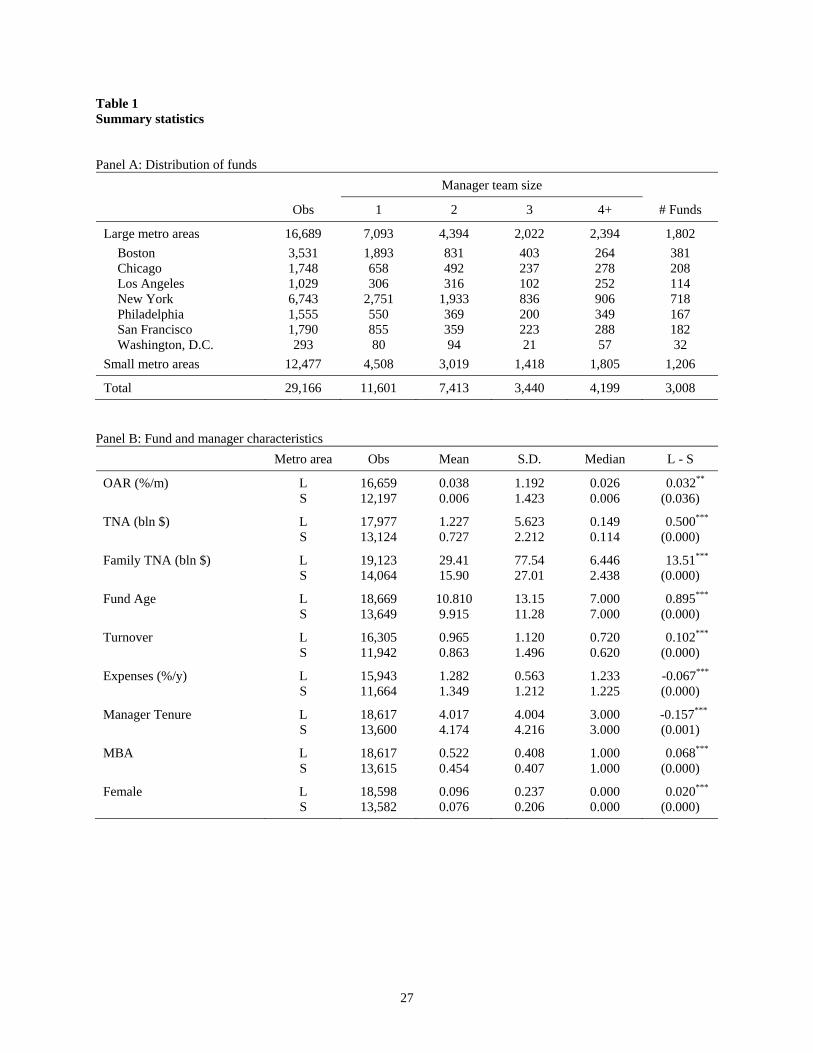
Table 1 provides the detailed summary statistics. Panel A shows the distribution of funds

and fund managerial structure across each of the seven largest U.S. metro areas and other

locations. Large population metro areas (LPAs) include 1,802 distinct funds; small population

metro areas (SPAs) – 1,206 funds. New York has the largest number of funds – 718, while

Washington, D.C. the smallest – only 32. Across funds with manager team sizes, we can note

that single-managed funds constitute the majority in most of the locations except Los Angeles 8 Smoothing of twelve-month fund returns is common in the literature (e.g., Cassar and Gerakos, 2011; Aiken, Clifford, and Ellis, 2013; Chen, Hong, Jiang, and Kubik, 2013). Our test results based on winsorized risk-adjusted returns, which are similar to those in this study, are available on request.

11

and Washington, D.C., where the most common form of managerial structure is two-manager

teams. Boston appears to have the largest fraction of single-managed funds among all other

largest metro areas: it exceeds 50% of all fund observations.

Panel B of Table 1 shows basic statistics, such as the mean, standard deviation, median,

and the difference in the means test, for fund and manager characteristics in large and small

metro areas. Consistent with Christoffersen and Sarkissian (2009), we find that objective-

adjusted returns (OARs) in larger metro areas are on average significantly higher than in smaller

locations. Large metro area funds also tend to be larger and older, belong to larger fund families,

have much higher annual turnover, but lower expense ratio than small metro area funds. There

are significant differences in managerial characteristics across locations as well. The manager

tenure with the same fund in large metro areas is significantly lower than that in smaller metro

areas, although the median of three years is the same across all locations. Also, on average, funds

in larger cities have more managers with an MBA degree and more females.

3. Preliminary Evidence

In the fund management industry, skills, knowledge, as well as networking ability of each

team member can be of great importance to fund performance. That is, if teams in the financial

industry are able to achieve diversification of style and judgment, as argued by Barry and Starks

(1984), and Sah and Stiglitz (1986, 1991), then the value of having a team must be larger when

each individual has a higher potential to enhance the overall knowledge and resource base of the

group. Numerous studies have shown that those conditions are more readily available in larger

urban agglomerations. This could be due to a more vibrant pool of skilled workers, who find

appropriate jobs easier in larger metro areas, as argued by Helsley and Strange (1990, 1991).

Alternatively, it could be due to an easier knowledge transfer, faster and more diverse business

and social connections, and potential access to private information found in larger cities, as

12

argued by Jacobs (1969), Glaeser (1999), and Christoffersen and Sarkissian (2009). These two

explanations are not mutually exclusive, and our task is to provide sufficient evidence for one or

both potential reasons.

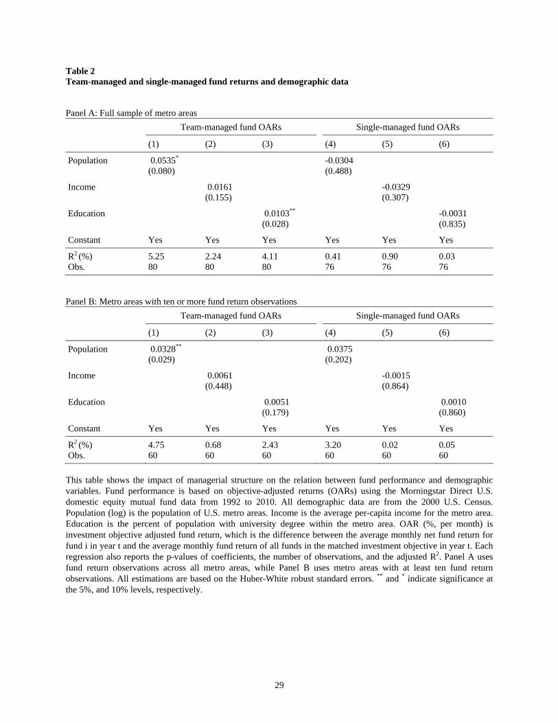
In Table 2 we regress objective-adjusted returns of team-managed and single-managed

funds on the metro area population as well as on the two other demographic variables: average

per capita income (in thousand U.S. dollars) and education level (the percent of population with

a university degree) in each metropolitan area. In regressions, the population data are

transformed logarithmically. All estimations are based on the Huber-White robust standard

errors. Panel A uses fund returns across all metro areas with team-managed and single-managed

fund return observations. There are 80 locations with team-managed fund returns and 76 single-

managed. In Panel B we include only those metro areas that have at least ten fund return

observations. The main conclusion from these two panels is that, indeed, there is a positive and

significant relation between fund performance and metro area population size. Yet, there is no

any relation between fund returns and the average income. There is also some indication that

education level of the metro area may be conductive to team-managed fund performance. The

performance of single-managed funds shows no relation to any of the three demographic

variables. Thus, Table 2 results highlight a distinct impact of metro areas with different

population sizes and, to some extent, average education level to the performance of team-

managed funds.

In general, larger cities are associated with larger educational opportunities. Indeed,

Table 2 shows a positive relation between the log of population and percent of university degree

holders in 91 U.S. metro areas that have domestic equity mutual fund data in our 1992-2010

sample period. This relation is significant at the 5% level. In our data, the median percent of

university degree holders across 91 cities is 30.5%. We denote cities with education level

exceeding (not exceeding) the sample median as high (low) education areas, HEA (LEA).

Among our sample of seven large metro areas, four, namely: Boston, New York, Washington,

D.C., and San Francisco also have above median education level. Among cities with high

13

education level but outside our set of the largest metro areas, Atlanta, Denver, and Minneapolis,

also provide substantial number of fund return observations. In fact, these cities also belong to

the largest urban areas in the United States – more precisely, the top 20% in our sample of 91

areas with mutual fund companies. Therefore, in some of the follow-up tests, we perform

estimation on metro area sub-sample splits by both population size and education level.

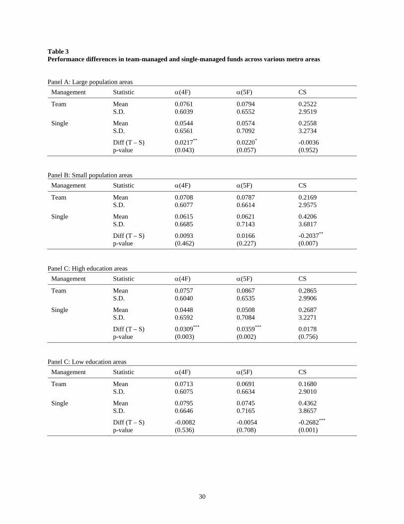
In Table 3 provides the first formal tests of the differences in team-managed fund

performance across locations using our three performance measures, (4F), (5F), and CS. It

shows the means and standard deviations of these metrics and the difference in means test

between team-managed and single-managed funds returns for each location set. Panels A and B

report these statistics for large and small metro areas, respectively. We can see that the

differences in (4F) and (5F) between team-managed and single-managed funds are significant

in large metro areas. In economic terms, in large metro areas the risk-adjusted returns of team-

managed funds are 26 bps (0.0217×12 or 0.220×12) per year higher than similar returns of

single-managed funds. However, we observe no differences in (4F) and (5F) between team-

managed and single-managed funds in small cities. In addition, while the difference in CS

measure is negligible in large cities, team-managed funds significantly underperform their

single-managed counterparts in smaller metro areas.

Panels C and D in Table 3 report our performance statistics for high and low education

metro areas, respectively. The overall picture is similar to that in Panels A and B. Again, the

differences in (4F) and (5F) between team-managed and single-managed funds are

economically and statistically significant in large metro areas but not small ones. The magnitude

of the two risk-adjusted returns of team-managed funds in high education areas is 37-43 bps per

year higher than that for similar returns of single-managed funds. The difference in CS measure

is insignificant in Panel C, yet is negative and highly significant in Panel D, indicating

underperformance of team-managed funds in low education metro areas. Thus, Table 3 shows

directly, albeit without accounting for fund and manager characteristics, that team management

14

in the fund industry is associated with better performance only in large and more educated metro

areas but not in smaller and low education cities.

4. Main Empirical Tests

We now move to examining the relation between fund performance and team

management in large and small metro areas while controlling for the full set of lagged fund and

managerial characteristics.9 The regression model is as follows:

t,it,it,it,it,it,i eFEControls_MgrControls_FundTeamccPerf 31211110 , (4)

where Perfi,t is one of our three measures of fund performance, Team is the dummy for team-

manager funds, Fund_Controls and Mgr_Controls are fund- and manager-specific characteristics,

respectively. The fixed effects, FE, include the year times the investment objective effects, fund

family fixed effects, as well as the metro area dummies.10 The fund characteristics are lagged by

one period to exclude their contemporaneous influence on fund alphas. We also use an

alternative specification to Eq. (4) to estimate directly the impact of the team management

between large and small metro areas and between metro areas with high and low average

education level. These regressions are:

t,iit,iit,it,i eFEandControlsSPATeamcLPATeamccPerf δ12110 , (5)

and

t,iit,iit,it,i eFEandControlsLEATeamcHEATeamccPerf δ12110 , (6)

9 Lagging the Team dummy precludes the look-ahead bias in our estimations. 10 Metropolitan area fixed effects are included given the evidence that mutual fund returns are different across geographic locations (see Coval and Moskowitz, 2001; Christoffersen and Sarkissian, 2009).

15

where Team×LPA and Team×SPA are the interactive variables of the team dummy with

dummies for large and small population metro areas, while Team×HEA and Team×LEA are

those for high and low education areas. In models (5) and (6) the sets of control variables and

fixed effects are the same as in model (4).

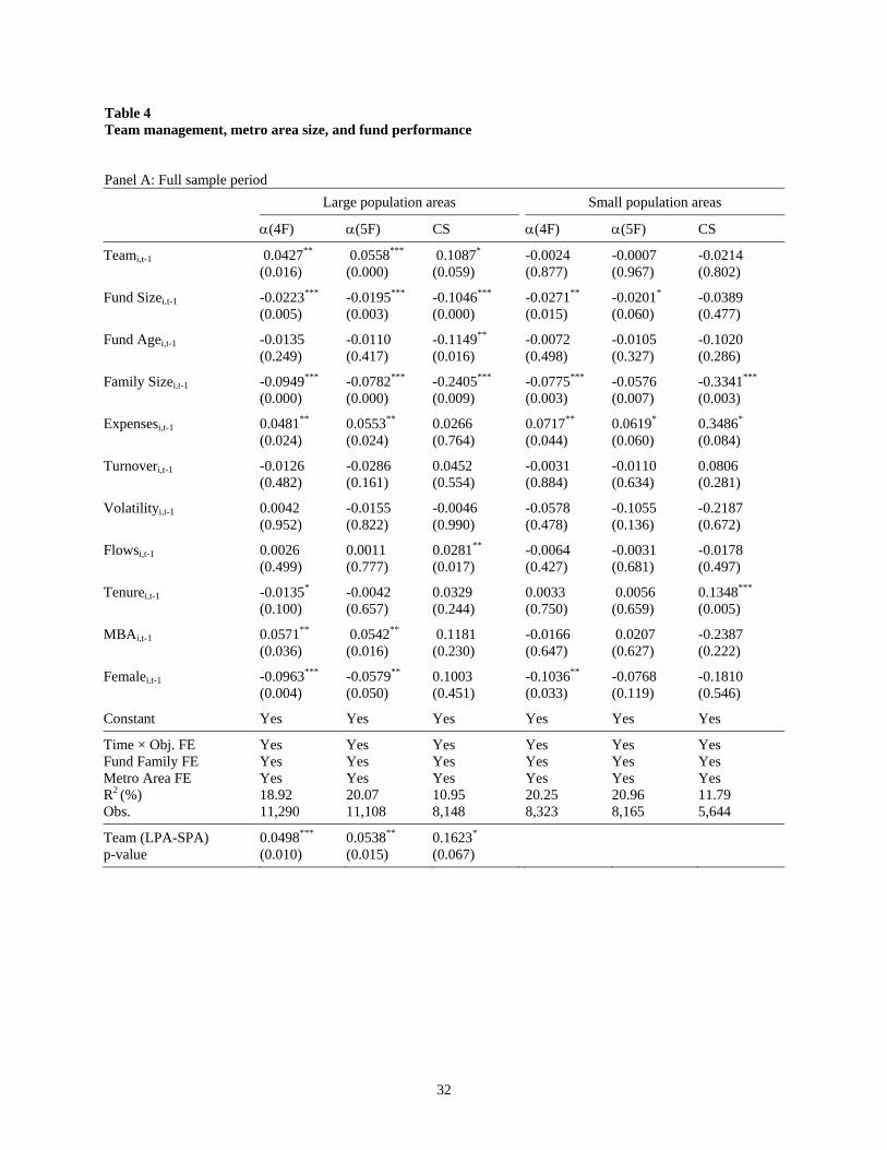
4.1. Teams, location, and fund performance

Table 4 shows the estimates from panel regressions of (4F), (5F), and CS on Team

dummy and other controls using Eq. (4) across locations based on metro area population size. It

also reports the p-values of coefficients, the number of observations, and the R-squared. The

standard errors are clustered by fund and year. Panel A shows the full sample period results. The

first three columns show the regression estimates for the largest seven metro areas. The Team

coefficient is positive and highly significant in all three specifications. In economic terms, in

large metro areas team-managed funds outperform their single-managed counterparts by 51-67

bps per year based on fund alphas and 130 bps per year based on the characteristic selectivity. In

the last thee columns of Panel A, which show regression estimates for smaller metro areas, we

can see that across all specifications the coefficient on Team is statistically zero and

economically very small as well. This implies that on average teams add no gains to performance

for funds located outside the largest seven U.S. metro areas. Moreover, the last two lines in the

panel give the difference in the Team coefficient across metro areas, Team (LPA-SPA), and the

corresponding p-value of the F-test for the equality of estimates. Here, we see that the risk-

adjusted return difference between team-managed funds located in large metro areas and those in

small metro is again economically and statistically significant at the 5% level. The difference in

the corresponding CS measures is significant at the 10% level.

It is worthwhile to note that out of the eleven independent variables in regression model

(4), the impact of the Team dummy is the most different one between large and small metro

areas. All other variables have very similar influence on three fund performance metrics,

16

irrespective of the location of fund advisors. We also note that the overall fit of the regression

with CS as a dependent variable is much lower than that with risk-adjusted returns.

Panel B of Table 4 shows the results for the 1992-2004 and 2005-2010 sub-periods. This

unequal time period split yields comparable number of fund-year observations in both sub-

samples. In this panel, we use estimations based on Eq. (5). For conciseness, we do not report the

estimates on fund and manager controls. Our results are very similar to those over the whole

sample period in Panel A. As before, in large metro areas, irrespective of the performance

measure and the time period, the Team coefficient is always positive and significant both

economically and statistically, except for the CS measure prior to 2005. Note that the reduction

in statistical significance in this case is largely due to the smaller sample size. Yet, again similar

to the full sample results, there is no any evidence of performance benefits among team-managed

funds in small metro areas.

Recall that in Table 3 we observe that the impact of team management on fund returns

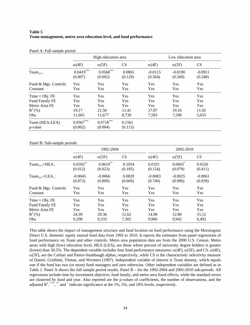
varies also across cities’ education levels. Therefore, in Table 5 we conduct tests, similar to those

in Table 4, but splitting the sample by high and low education metro areas. In this Table, we

report only the coefficients on the variables involving the Team dummy, although all controls are

similar to those in Table 4. Panel A reports the full sample period results. Consistent with Table

3 findings, team-managed funds show significant outperformance only in high education areas.

The economic impact of team management for risk-adjusted returns is 50-68 bps, which is

remarkably similar to the corresponding estimates in Panel A of Table 4. The CS measure is

significant economically, but not statistically. In contrast, the Team dummy is not only

statistically insignificant for low education level areas but also takes economically non-trivial

negative values in these locations for all three performance metrics. The last two lines in the

panel, show that team-managed funds in high education areas outperform their peers in low

education areas by as much as 68-86 bps per year based on (4F) and (5F).

Panel B of Table 5 shows the regression results using Eq. (6) for the 1992-2004 and

2005-2010 sub-periods. The format of this panel is identical to that of Panel B of Table 4. The

17

outcome of estimations is also similar to previous findings. In both sub-periods, the coefficient

on the interactive term, Team×HEA, is positive and significant for all three measures of fund

performance (except for the CS measure statistically), while that on Team×LEA is small and

insignificant. This again reflects the fact that teams provide no additional value to fund

performance outside a very select group of cities with highly educated average workforce. Since

these metro areas are still large urban agglomerations, all our subsequent sample splits are done

using only metro area population size.

While our finding on the outperformance of team-managed funds in large or highly

educated metro areas withstands sub-period tests, it is also necessary to observe whether this

outcome is concentrated in certain types of funds. One can expect that the significance of team

management should be positively related to the ability of funds collect information on hard-to-

value assets. Since teams indeed add to fund returns in larger cities, team-managed funds located

in these metro areas should be in a relatively better positioned in dealing with growth stocks than

those with steady dividend income.

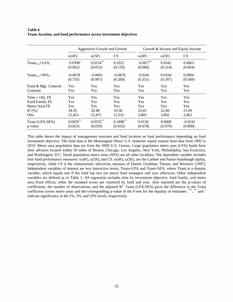
To examine this, in Table 6 we show tests on how managerial structure impacts funds

returns in different locations across two funds groups composed from four original funds

investment objectives. The first group, which we call Growth funds, contains aggressive growth

and growth funds; the second group, which we call Income funds, contains growth & income and

income funds. All the econometric specifications of regressions are the same as in Table 4, Panel

B, that is are based on Eq. (5). The table also reports the difference in the Team coefficient

across the two metro area groups and the corresponding p-value of the F-test for the equality of

estimates. We can see that team management is uniformly more profound in large metro areas

for Growth funds only. The coefficients on Team×LPA is positive and statistically significant for

all three performance metrics (except statistically for the CS measure). Its economic importance

for risk-adjusted returns exceeds 48 bps per year. The coefficient on Team×SPA is effectively

zero. In contrast, for the Income group of funds, the team-managed funds in both large and small

metro areas show comparable performance relative to the corresponding single-managed funds.

18

Thus, Tables 4-6 provide comprehensive statistical evidence that the benefits of team

management are widely different across urban agglomerations with different population size.

The gain in risk-adjusted returns from the team-based approach in portfolio management is

significantly higher among those funds, whose advisors are located in larger and more educated

metro areas. This result holds in both the earlier and the later sample periods and is manifests

itself more profoundly among funds with growth investment objectives. Our findings support

Sharpe (1981) arguments and provide novel evidence that group decision-making is more

beneficial in such environments where their members are more likely to acquire and use

knowledge, skills, and establish business connections. In the finance industry in general and fund

industry in particular, this becomes more achievable in larger and more affluent cities.

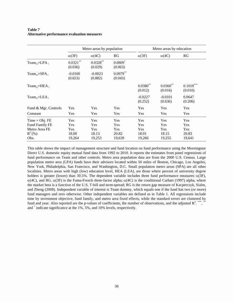
4.2. Alternative Performance Measures

In this section, we repeat our main estimations using alternative performance evaluation

models. We consider three new metrics. The first one is the Fama-French three-factor alpha

(3F), computed from

titititmiiti eHMLhSMBsrF)r ,,, 3( , (7)

where, as before, ri,t is the monthly gross fund return less the risk-free rate.

The second alternative is the conditional Carhart (1997) alpha, (4C). We use a

specification, where market beta is modeled as a linear function of instruments, as in Ferson and

Schadt (1996), namely:

tiTermttm

Termi

Tbillttm

Tbillititititmiiti eZrbZrbUMDmHMLhSMBsrCr ,1,1,,, )4( . (8)

In Eq. (8), TbilltZ 1 and Term

tZ 1 are the two lagged (demeaned) public information variables: the one-

month U.S. Treasury bill rate (T-bill) and the term-structure spread (Term), defined as the

19

difference in yields on the 10-year U.S. government bond and three-month U.S. T-bill. We again

trim the top and bottom 1% of distribution of both risk-adjusted returns.

The third alternative is the return gap, RG, of Kacperczyk, Sialm, and Zheng (2008).

Return gap is which is defined as the difference between the reported fund return and the return

of a portfolio that invests in the previously disclosed holdings net of expenses. Table 7 shows the

estimation results with alternative performance measures. In the first three columns of the table

the estimations are based on Eq. (5), where team-management impact is compared between large

and small population size metro areas. In the last three columns of the table the estimations are

based on Eq. (6), where team-management impact is compared between high and low education

metro areas. Our results are very similar to previous findings for (3F) and (4C). We see highly

positive and significant coefficients on Team×LPA and Team×HEA but not Team×SPA and

Team×LEA for these performance measures. Moreover, a similar pattern is observed for the

return gap in column 6. Only in column 3 for the RG measure the coefficient on interactive Team

variable shows no difference between locations. Thus, we can state that the evidence on

outperformance of team-managed funds in larger and more educated cities relative to their

counterparts in smaller places depends very little on the chosen performance evaluation metrics.

4.3. Team Formation and De-Formation

There are two potential issues with our previous tests. First, we do not differentiate

between teams of different sizes. Hamilton, Nickerson, and Owan (2003) and Patel and

Sarkissian (2016) show that team size has a non-linear relation to firm performance. Second, in

those tests we do not maintain the same fund managers within the team. It is clear that for a

given team, there can be differences in both collaboration gains and coordination costs if over

time the members comprising the team are different people or are the same individuals. Our next

tests address these points by comparing the returns of team-managed and single-managed funds

over time with their own past performance. Therefore, we now focus our attention only on those

team-managed and single-managed funds that change their managerial structure within our 19

20

year sample period, and call these instances as team-formation and team de-formation. All funds

with a constant managerial structure throughout the sample period are dropped. This condition

significantly lowers the overall number of available observations.

We define the team formation year to be if fund i is team-managed at times t, t-1,…, t-,

but was single-managed at time t--1. Similarly, the team de-formation year is if fund i is

single-managed at times t, t-1,…, t-, but was team-managed at time t--1. Figure 3 shows the

stability of the managerial structure is from the team formation and de-formation years. Plot A

depicts the average percent of the same managers in a team after the team formation for the

given fund. The first year of team formation is shown with 100%. However, by the second year,

about 25% of team members are replaced. The subsequent changes in team members are not so

drastic, but the overall number of the same managers tends to decrease slowly. Plot B gives the

average percent of the same single manager after team de-formation with the given fund. Here,

the initial change in the manager at year two is constitutes only about 10%. In subsequent years,

the change of the single manager becomes an even rarer event.

Table 8 examines the relation between the formation and de-formation of team-

management and fund performance across metro areas of different population sizes. New (old)

team formation denotes funds that became team-managed up to three (four or more) years ago,

while new (old) team de-formation denotes funds that became single-managed up to three (four

or more) years ago. It also shows the p-value for the difference test between old and new team

formation/de-formation, Diff (Old – New). Panel A presents the results for the same number of

managers. We can see that the average risk-adjusted returns for teams in large metro areas that

were formed more than four years ago are significantly higher than those for teams formed more

recently for all three performance metrics. The average difference is about 53 bps for (4F) and

(5F) and 40 bps for the CS measure. There are no significant differences between single-

managed funds which are formed recently or late.

Panel B of Table 8 gives the test results for the same portfolio managers within each

team. The number of observations in this panel is smaller than that in Panel A since substantial

21

changes occur over time among team members even within teams of the same size. In spite of

this difference, the overall pattern of team-managed and single-managed funds performance is

similar to that in Panel A. Again, we can see that (4F), (5F), and CS for teams in large metro

areas formed more than four years ago are much larger than the corresponding returns for teams

formed in the last three years. Moreover, the magnitude of these differences is even higher than

before, reaching 65 bps for (4F), 70 bps for (5F), and 44 bps for CS. Thus, Table 6 results

have very important implication to our understanding on how teams improve on fund

performance in larger cities. It appears that it is not the inner initial set of skills of group

members in larger cities that plays a crucial role there, as suggested by Helsley and Strange

(1990, 1991). Rather, it is the wider set of opportunities which large cities offer for knowledge

collection and production. It is not surprising then that these unique knowledge dissemination

and learning possibilities in large metro areas become revealed in team work only over time,

which is consistent with Jacobs (1969), Lucas (1988), Glaeser (1999), and others.

5. Portfolio Holdings

Numerous studies document certain portfolio holding patterns among outperforming

mutual funds. For example, Kacperczyk, Sialm, and Zheng (2004) find that funds with more

concentrated investments post higher returns than those investing in more diversified portfolios.

It is known that equity mutual funds hold only a small fraction of their holdings in cash, T-bills,

and other fixed-income securities. Therefore, funds with lower number of holdings are expected

to post higher average returns. Given wide performance differences among team-managed funds

between large and small metro areas, one should expect to similar patterns in their portfolio

holdings as well.

Table 9 reports the relation of management structure on fund holdings across the two

location sets. The econometric framework is similar to Eq. (5), except that the dependent

22

variable now is the log of portfolio holdings for each fund-year. As before, all regression

specifications include time by investment objective, fund family, and metro area fixed effects,

and the standard errors are clustered by fund and year. The first three regressions use the full

sample period and different sets of control variables. We can see that, irrespective of controls,

the coefficients on both interactive Team terms are positive and significant. This shows as in

Patel and Sarkissian (2016) that team-managed funds in general hold more securities. What is

much more important in this study, however, is that the magnitude as well as statistical

significance of the coefficient on Team×LPA is consistently lower than that on Team×SPA. The

F-test results at the bottom of the table highlight the difference in these coefficients. The sample

period slit in the last two columns of the table presents the same pattern. The only exception is

that, due to the significantly smaller sample size, the F-tests in these cases do not record

statistical significance in the difference. This means that fund manager teams in large cities hold

relatively smaller number of securities than comparative teams managing similar funds in

smaller metro areas. After analyzing the composition of aggregate holdings, we observe that

team-managed funds in large cities invest significantly more in stocks and significantly less in

bonds and cash than team-managed funds in smaller metro areas.11

With similar reasoning, we should also expect differences in team-managed funds across

locations in terms of active share holdings. Cremers and Petajisto (2009) show that active share

holdings, which represents the proportion of holdings that differs from the benchmark index

holdings, is higher among better performing funds. Therefore, active share among team-managed

funds in larger should be higher than that among similar funds in smaller areas. Table 10

illustrates the test results. In this table the regression framework is again based on Eq. (5) but

fund performance is substituted with active share for each fund-year.12 The structure of the table

is similar to that in Table 9. The first three columns show the estimation results for various sets

of control variable, while the last two perform sub-period estimation. We find that the coefficient

11 These results are available on request. 12 The active share data is kindly provided by Martijn Cremers.

23

on the interactive Team dummy in large metro areas is small and insignificant in all five columns

of the table, implying that active share among team-managed and single-managed funds in large

cities is about the same. Yet, the coefficient on Team×SPA is negative and significant also across

all estimations, and the last two lines in the table indicate that the difference with Team×LPA is

significant too. This suggests that team-managed funds in smaller metro areas have lower active

share with respect to both team-managed funds in large cities as well as practically all single-

managed funds on average.

Thus, Tables 9-10 show that, consistent with outperformance results among team-

managed funds in large metro areas documented in earlier sections, their portfolio holdings also

show quite distinct patterns. These funds have a much higher propensity of holding more

concentrated portfolios as well as higher active shares than team-managed funds in smaller metro

areas.

6. Conclusions

In this paper, we connect urban economics and organization structure. A large number of

studies in both strands of literature suggest that better information processing environment can

enhance firm productivity. The urban economics literature relates the areas with larger

population as more conductive to learning and knowledge spillover. The literature on

organization structure suggests that teams generate better solutions from diversified knowledge

and skills of their members. As a result, it becomes quite suggestive that team management must

lead to higher gains in large metropolitan areas.

Indeed, using U.S. equity mutual fund and demographic data, we find that the benefits of

team-based managerial approach are drastically different across locations. Team-managed funds

outperform single-managed funds in larger metro areas but not in small ones. This outcome is

robust across various fund performance metrics, sub-sample periods, and the inclusion of fund

24

and manager characteristics controls. Moreover, we show that superior performance of team-

managed funds in large metro areas in present only among portfolio managers with substantial

team-work experience. There are no differences in risk-adjusted and characteristic-adjusted

returns among recently formed teams of funds managers in relation to single managers,

irrespective of fund location, implying that the initial skills of group members are not very

important. We also observe differences in security holding of team-managed funds between large

and small cities. Team-managed funds in large agglomerations hold more concentrated portfolios

and have higher active share. Therefore, we interpret our results as evidence of the positive

externality of larger cities for team-based organizational structures through more accessible

information sources, larger social and business networks, and better learning opportunities.

References:

Adams, R., and D. Ferreira, 2010, Moderation in groups: Evidence from betting on ice break-ups in Alaska, Review of Economic Studies 77, 882-913.

Aiken, A., C. Clifford, and J. Ellis, 2013, Hedge funds and discretionary liquidity restrictions, Review of Financial Studies 26, 208-243.

Alchian, A., and H. Demsetz, 1972, Production, information costs and economic organization, American Economic Review 62, 777-705.

Bar, M., A. Kempf, and S. Ruenzi, 2011, Is a team different from the sum of its parts? Evidence from mutual fund managers, Review of Finance 15, 359-396.

Barber B., and T. Odean, 2001, Boys will be boys: Gender, overconfidence, and common stock investment, Quarterly Journal of Economics 116, 261-292.

Barber, B., C. Heath, and T. Odean, 2003, Good reasons sell: Reason-based choice among group and individual investors in the stock market, Management Science 49, 1636-1652.

Barry, C., and L. Starks, 1984, Investment management and risk sharing with multiple managers, Journal of Finance 39, 477-491.

Blinder, A., and J. Morgan, 2005, Are two heads better than one? Monetary policy by committee, Journal of Money, Credit and Banking 37, 789-811.

Carhart, M., 1997, On persistence in mutual fund performance, Journal of Finance 52, 57-82.

Cassar, G., and J. Gerakos, 2011, Hedge funds: Pricing controls and the smoothing of self-reported returns, Review of Financial Studies, 24, 1698-1734.

25

Chen, J., H. Hong, M. Huang, and J. Kubik, 2004, Does fund size erode mutual fund performance? The role of liquidity and organization, American Economic Review 94, 1276-1302.

Chen, J., H. Hong, W. Jiang, and J. Kubik, 2013, Outsourcing mutual fund management: Firm boundaries, incentives and performance, Journal of Finance 68, 523–558.

Chevalier, J., and G. Ellison, 1999, Are some mutual fund managers better than others? Cross-sectional patterns in behavior and performance, Journal of Finance 54, 875-899.

Christoffersen, S., and S. Sarkissian, 2009, City size and fund performance, Journal of Financial Economics 92, 252-275.

Combes, P-P., G. Duranton, L. Gobillon, D. Puga, and S. Roux, 2012, The productivity advantages of large cities: Distinguishing agglomeration from firm selection, Econometrica 80, 2543-2594.

Cooper, D., and J. Kagel, 2004, Are two heads better than one? Team versus individual play in signaling games, American Economic Review 95, 477-509.

Coval, J., and T. Moskowitz, 2001, The geography of investment: Informed trading and asset prices, Journal of Political Economy 109, 811-841.

Cremers, M., and A. Petajisto, 2009, How active is your fund manager? A new measure that predicts performance, Review of Financial Studies 22, 3329-3365.

Ferson, W., and R. Schadt, 1996, Measuring fund strategy and performance in changing economic conditions, Journal of Finance 51, 425-461.

Feri, F., B. Irlenbusch, and M. Sutter, 2010, Efficiency gains from team-based coordination – large-scale experimental evidence, American Economic Review 100, 1892-1912.

Glaeser, E., 1999, Learning in cities, Journal of Urban Economics 46, 254-277.

Glaeser, E., H. Kallal, J. Scheinkman, and A. Shleifer, 1992, Growth in cities, Journal of Political Economy, 100, 1126-1152.

Holmstrom, B., 1982, Moral hazard in teams, Bell Journal of Economics, 13, 324-340.

Hamilton, B., J. Nickerson, and H. Owan, 2003, Team incentives and worker heterogeneity: An empirical analysis of the impact of teams on productivity and participation, Journal of Political Economy 111, 465-497.

Helsley, R., and W. Strange, 1990, Matching and agglomeration economies in a system of cities, Regional Science and Urban Economics 20, 198-212.

Helsley, R., and W. Strange, 1991, Agglomeration economies and urban capital markets, Journal of Urban Economics 29, 96-11.

Hong, H., J. Kubik, and J. Stein, 2005, Thy neighbor’s portfolio: word-of- mouth effects in the holdings and trades of money managers, Journal of Finance 60, 2801-2824.

Jacobs, J., 1969, The Economy of Cities, Vintage, New York.

Kacperczyk, M., C. Sialm, and L. Zheng, 2008, Unobserved actions of mutual funds, Review of Financial Studies 21, 2379-2416.

26

Linnainmaa, J., 2013, Reverse survivorship bias, Journal of Finance 68, 789-813.

Lucas, R., 1988, On the mechanics of economic development, Journal of Monetary Economics 22, 3-42.

Massa, M., J. Reuter, and E. Zitzewitz, 2010, When should firms share credit with employees? Evidence from anonymously managed mutual funds, Journal of Financial Economics 95, 400-424.

Melitz, M., 2003, The impact of trade on intra-industry reallocations and aggregate industry productivity, Econometrica, 71, 1695-1725.

Nalbantian, H., and A. Schotter, 1997, Productivity under group incentives: An experimental study, American Economic Review 87, 314-341.

Patel, S., and S. Sarkissian, 2016, To group or not to group? Evidence from mutual funds databases, Journal of Financial and Quantitative Analysis, forthcoming.

Rosenthal, S., and W. Strange, 2004, Evidence on the nature and sources of agglomeration Economies, in Handbook of Regional and Urban Economics, Vol. 4, Eds. V. Henderson and J.-F. Thisse, Amsterdam: North-Holland, 2119-2171.

Sah, R., and J. Stiglitz, 1986, The architecture of economic systems: Hierarchies and polyarchies, American Economic Review 76, 716–727.

Sah, R., and J. Stiglitz, 1991, The quality of managers in centralized versus decentralized organizations, Quarterly Journal of Economics 106, 289–295.

Smith, A., 1776, An Inquiry Into the Nature and Causes of the Wealth of Nations. London: Printed for W. Strahan and T. Cadell.

Sharpe, W., 1981, Decentralized investment management, Journal of Finance 36, 217-234.

Wheeler, C., 2001, Search, sorting, and urban agglomeration, Journal of Labor Economics 19, 879-899.

27

Table 1 Summary statistics Panel A: Distribution of funds

Manager team size

Obs 1 2 3 4+ # Funds

Large metro areas 16,689 7,093 4,394 2,022 2,394 1,802

Boston 3,531 1,893 831 403 264 381 Chicago 1,748 658 492 237 278 208 Los Angeles 1,029 306 316 102 252 114 New York 6,743 2,751 1,933 836 906 718 Philadelphia 1,555 550 369 200 349 167 San Francisco 1,790 855 359 223 288 182 Washington, D.C. 293 80 94 21 57 32

Small metro areas 12,477 4,508 3,019 1,418 1,805 1,206

Total 29,166 11,601 7,413 3,440 4,199 3,008

Panel B: Fund and manager characteristics

Metro area Obs Mean S.D. Median L - S

OAR (%/m) L 16,659 0.038 1.192 0.026 0.032** S 12,197 0.006 1.423 0.006 (0.036)

TNA (bln $) L 17,977 1.227 5.623 0.149 0.500*** S 13,124 0.727 2.212 0.114 (0.000)

Family TNA (bln $) L 19,123 29.41 77.54 6.446 13.51*** S 14,064 15.90 27.01 2.438 (0.000)

Fund Age L 18,669 10.810 13.15 7.000 0.895*** S 13,649 9.915 11.28 7.000 (0.000)

Turnover L 16,305 0.965 1.120 0.720 0.102*** S 11,942 0.863 1.496 0.620 (0.000)

Expenses (%/y) L 15,943 1.282 0.563 1.233 -0.067*** S 11,664 1.349 1.212 1.225 (0.000)

Manager Tenure L 18,617 4.017 4.004 3.000 -0.157*** S 13,600 4.174 4.216 3.000 (0.001)

MBA L 18,617 0.522 0.408 1.000 0.068*** S 13,615 0.454 0.407 1.000 (0.000)

Female L 18,598 0.096 0.237 0.000 0.020*** S 13,582 0.076 0.206 0.000 (0.000)

28

Table 1 (continued) This table gives the summary statistics of domestic equity mutual funds in the United States from 1992 to 2010 for large and small metro areas. The fund data comes from Morningstar Direct. The metro areas are classified based on the 2000 U.S. Census. Panel A shows distribution of funds across the largest metro areas and fund manager team size. Panel B gives fund and manager characteristics between the two locations and provides their difference test. OAR (%, per month) is the investment objective adjusted fund return, which is the difference between the average monthly net fund return for fund i in year t and the average monthly fund return of all funds in the matched investment objective in year t. TNA ($, billions) is the total net asset under management of fund i in year t. Family TNA ($, billions) is the total net asset under management of family of fund i in year t. Fund Age (years) is the difference between fund i’s inception year and the current year t. Turnover is the minimum of aggregated sales or aggregated purchases of securities of the year divided by the average 12-month total net assets of the fund. Expenses (%) is the annual total expense ratio of the fund i in year t. Manager Tenure (years) is the number of years the fund manager remains with the fund i at time t. MBA is defined as a proportion of managers in a fund with a MBA degree. Female is defined as a proportion of female managers in a fund. In case of teams, the average of Tenure is taken. *** and ** indicate significance at the 1%, and 5% levels, respectively.

29

Table 2 Team-managed and single-managed fund returns and demographic data Panel A: Full sample of metro areas

Team-managed fund OARs Single-managed fund OARs

(1) (2) (3) (4) (5) (6)

Population 0.0535* -0.0304 (0.080) (0.488)

Income 0.0161 -0.0329 (0.155) (0.307)

Education 0.0103** -0.0031 (0.028) (0.835)

Constant Yes Yes Yes Yes Yes Yes

R2 (%) 5.25 2.24 4.11 0.41 0.90 0.03 Obs. 80 80 80 76 76 76

Panel B: Metro areas with ten or more fund return observations

Team-managed fund OARs Single-managed fund OARs

(1) (2) (3) (4) (5) (6)

Population 0.0328** 0.0375 (0.029) (0.202)

Income 0.0061 -0.0015 (0.448) (0.864)

Education 0.0051 0.0010 (0.179) (0.860)


R2 (%) 4.75 0.68 2.43 3.20 0.02 0.05 Obs. 60 60 60 60 60 60

This table shows the impact of managerial structure on the relation between fund performance and demographic variables. Fund performance is based on objective-adjusted returns (OARs) using the Morningstar Direct U.S. domestic equity mutual fund data from 1992 to 2010. All demographic data are from the 2000 U.S. Census. Population (log) is the population of U.S. metro areas. Income is the average per-capita income for the metro area. Education is the percent of population with university degree within the metro area. OAR (%, per month) is investment objective adjusted fund return, which is the difference between the average monthly net fund return for fund i in year t and the average monthly fund return of all funds in the matched investment objective in year t. Each regression also reports the p-values of coefficients, the number of observations, and the adjusted R2. Panel A uses fund return observations across all metro areas, while Panel B uses metro areas with at least ten fund return observations. All estimations are based on the Huber-White robust standard errors. ** and * indicate significance at the 5%, and 10% levels, respectively.

30

Table 3 Performance differences in team-managed and single-managed funds across various metro areas Panel A: Large population areas

Management Statistic (4F) (5F) CS

Team Mean 0.0761 0.0794 0.2522 S.D. 0.6039 0.6552 2.9519

Single Mean 0.0544 0.0574 0.2558 S.D. 0.6561 0.7092 3.2734

Diff (T – S) 0.0217** 0.0220* -0.0036 p-value (0.043) (0.057) (0.952)

Panel B: Small population areas


Team Mean 0.0708 0.0787 0.2169 S.D. 0.6077 0.6614 2.9575

Single Mean 0.0615 0.0621 0.4206 S.D. 0.6685 0.7143 3.6817

Diff (T – S) 0.0093 0.0166 -0.2037** p-value (0.462) (0.227) (0.007)

Panel C: High education areas


Team Mean 0.0757 0.0867 0.2865 S.D. 0.6040 0.6535 2.9906

Single Mean 0.0448 0.0508 0.2687 S.D. 0.6592 0.7084 3.2271

Diff (T – S) 0.0309*** 0.0359*** 0.0178 p-value (0.003) (0.002) (0.756)

Panel C: Low education areas


Team Mean 0.0713 0.0691 0.1680 S.D. 0.6075 0.6634 2.9010

Single Mean 0.0795 0.0745 0.4362 S.D. 0.6646 0.7165 3.8657

Diff (T – S) -0.0082 -0.0054 -0.2682*** p-value (0.536) (0.708) (0.001)

31

Table 3 (continued) This table shows the difference in fund performance between team-managed and single-managed funds metro areas of different size using the Morningstar Direct U.S. domestic equity mutual fund data from 1992 to 2010. Metro area population data are from the 2000 U.S. Census. Large population area funds have their advisors located within 50 miles of Boston, Chicago, Los Angeles, New York, Philadelphia, San Francisco, and Washington, D.C. (4F), (5F), are the Carhart and Pastor-Stambaugh alphas, respectively, while CS is the characteristic selectivity measure of Daniel, Grinblatt, Titman, and Wermers (1997). The p-values for the difference test between team-managed and single-managed funds, Diff (T –S), are in parentheses. ***, ** and * indicate significance at the 1%, 5%, and 10% levels, respectively.

32

Table 4 Team management, metro area size, and fund performance Panel A: Full sample period

Large population areas Small population areas

(4F) (5F) CS (4F) (5F) CS

Teami,t-1 0.0427** 0.0558*** 0.1087* -0.0024 -0.0007 -0.0214 (0.016) (0.000) (0.059) (0.877) (0.967) (0.802)

Fund Sizei,t-1 -0.0223*** -0.0195*** -0.1046*** -0.0271** -0.0201* -0.0389 (0.005) (0.003) (0.000) (0.015) (0.060) (0.477)

Fund Agei,t-1 -0.0135 -0.0110 -0.1149** -0.0072 -0.0105 -0.1020 (0.249) (0.417) (0.016) (0.498) (0.327) (0.286)

Family Sizei,t-1 -0.0949*** -0.0782*** -0.2405*** -0.0775*** -0.0576 -0.3341*** (0.000) (0.000) (0.009) (0.003) (0.007) (0.003)

Expensesi,t-1 0.0481** 0.0553** 0.0266 0.0717** 0.0619* 0.3486* (0.024) (0.024) (0.764) (0.044) (0.060) (0.084)

Turnoveri,t-1 -0.0126 -0.0286 0.0452 -0.0031 -0.0110 0.0806 (0.482) (0.161) (0.554) (0.884) (0.634) (0.281)

Volatilityi,t-1 0.0042 -0.0155 -0.0046 -0.0578 -0.1055 -0.2187 (0.952) (0.822) (0.990) (0.478) (0.136) (0.672)

Flowsi,t-1 0.0026 0.0011 0.0281** -0.0064 -0.0031 -0.0178 (0.499) (0.777) (0.017) (0.427) (0.681) (0.497)

Tenurei,t-1 -0.0135* -0.0042 0.0329 0.0033 0.0056 0.1348*** (0.100) (0.657) (0.244) (0.750) (0.659) (0.005)

MBAi,t-1 0.0571** 0.0542** 0.1181 -0.0166 0.0207 -0.2387 (0.036) (0.016) (0.230) (0.647) (0.627) (0.222)

Femalei,t-1 -0.0963*** -0.0579** 0.1003 -0.1036** -0.0768 -0.1810 (0.004) (0.050) (0.451) (0.033) (0.119) (0.546)


Time × Obj. FE Yes Yes Yes Yes Yes Yes Fund Family FE Yes Yes Yes Yes Yes Yes Metro Area FE Yes Yes Yes Yes Yes Yes R2 (%) 18.92 20.07 10.95 20.25 20.96 11.79 Obs. 11,290 11,108 8,148 8,323 8,165 5,644

Team (LPA-SPA) 0.0498*** 0.0538** 0.1623* p-value (0.010) (0.015) (0.067)

33

Table 4 (continued) Panel B: Sub-sample periods

1992-2004 2005-2010

(4F) (5F) CS (4F) (5F) CS

Teami,t-1×LPA i 0.0569** 0.0616** 0.1247 0.0363* 0.0471** 0.0779*** (0.026) (0.014) (0.247) (0.077) (0.031) (0.000)

Teami,t-1×SPA i 0.0063 -0.0006 0.0549 -0.0135 0.0187 -0.0399 (0.776) (0.982) (0.695) (0.615) (0.512) (0.740)

Fund & Mgr. Controls Yes Yes Yes Yes Yes Yes Constant Yes Yes Yes Yes Yes Yes


This table shows the impact of management structure and fund location on fund performance using the Morningstar Direct U.S. domestic equity mutual fund data from 1992 to 2010. It reports the estimates from panel regressions of fund performance on Team and other controls. Metro area population data are from the 2000 U.S. Census. Large metro area funds have their advisors located within 50 miles of Boston, Chicago, Los Angeles, New York, Philadelphia, San Francisco, and Washington, D.C. Small metro areas are all other localities. The dependent variable includes three fund performance measures(4F), (5F), and CS. (4F), (5F), are the Carhart and Pastor-Stambaugh alphas, respectively, while CS is the characteristic selectivity measure of Daniel, Grinblatt, Titman, and Wermers (1997). Independent variable of interest is Team dummy, which equals one if the fund has two (or more) fund managers and zero otherwise. Other independent variables are defined as in Table 1. Panel A shows the full sample period results. Team (LPA-SPA) gives the difference in the Team coefficient across metro areas and the corresponding p-value of the F-test for the equality of estimates. Panel B shows results for the 1992-2004 and 2005-2010 sub-periods. All regressions include time by investment objective, fund family, and metro area fixed effects, while the standard errors are clustered by fund and year. Also reported are the p-values of coefficients, the number of observations, and the adjusted R2. ***, ** and * indicate significance at the 1%, 5%, and 10% levels, respectively.

34

Table 5 Team management, metro area education level, and fund performance Panel A: Full sample period

High education area Low education area

(4F) (5F) CS (4F) (5F) CS

Teami,t-1 0.0419*** 0.0568*** 0.0865 -0.0115 -0.0190 -0.0911 (0.007) (0.002) (0.129) (0.564) (0.269) (0.248)



Team (HEA-LEA) 0.0567*** 0.0718*** 0.1561 p-value (0.002) (0.004) (0.113)

Panel B: Sub-sample periods

1992-2004 2005-2010

(4F) (5F) CS (4F) (5F) CS

Teami,t-1×HEA i 0.0593** 0.0610** 0.1054 0.0325 0.0603* 0.0526 (0.012) (0.023) (0.195) (0.154) (0.079) (0.411)

Teami,t-1×LEA i -0.0045 -0.0066 0.0820 -0.0083 -0.0025 -0.0061 (0.873) (0.809) (0.669) (0.740) (0.906) (0.939)



This table shows the impact of management structure and fund location on fund performance using the Morningstar Direct U.S. domestic equity mutual fund data from 1992 to 2010. It reports the estimates from panel regressions of fund performance on Team and other controls. Metro area population data are from the 2000 U.S. Census. Metro areas with high (low) education level, HEA (LEA), are those where percent of university degree holders is greater (lower) than 30.5%. The dependent variable includes four fund performance measures: (4F), (5F), and CS. (4F), (5F), are the Carhart and Pastor-Stambaugh alphas, respectively, while CS is the characteristic selectivity measure of Daniel, Grinblatt, Titman, and Wermers (1997). Independent variable of interest is Team dummy, which equals one if the fund has two (or more) fund managers and zero otherwise. Other independent variables are defined as in Table 1. Panel A shows the full sample period results, Panel B – for the 1992-2004 and 2005-2010 sub-periods. All regressions include time by investment objective, fund family, and metro area fixed effects, while the standard errors are clustered by fund and year. Also reported are the p-values of coefficients, the number of observations, and the adjusted R2. ***, ** and * indicate significance at the 1%, 5%, and 10% levels, respectively.

35

Table 6 Team, location, and fund performance across investment objectives

Aggressive Growth and Growth Growth & Income and Equity Income

(4F) (5F) CS (4F) (5F) CS

Teami,t-1×LPA i 0.0398* 0.0534** 0.1022 0.0477** 0.0342 0.0663 (0.062) (0.013) (0.129) (0.066) (0.214) (0.604)

Teami,t-1×SPA i -0.0078 -0.0001 -0.0876 0.0341 0.0334 0.0904 (0.735) (0.997) (0.269) (0.351) (0.397) (0.560)



Team (LPA-SPA) 0.0476** 0.0535** 0.1898** 0.0136 0.0008 -0.0241 p-value (0.023) (0.029) (0.032) (0.678) (0.979) (0.898)

This table shows the impact of management structure and fund location on fund performance depending on fund investment objective. The fund data is the Morningstar Direct U.S. domestic equity mutual fund data from 1992 to 2010. Metro area population data are from the 2000 U.S. Census. Large population metro area (LPA) funds have their advisors located within 50 miles of Boston, Chicago, Los Angeles, New York, Philadelphia, San Francisco, and Washington, D.C. Small population metro areas (SPA) are all other localities. The dependent variable includes four fund performance measures: (4F), (5F), and CS. (4F), (5F), are the Carhart and Pastor-Stambaugh alphas, respectively, while CS is the characteristic selectivity measure of Daniel, Grinblatt, Titman, and Wermers (1997). Independent variables of interest are two interactive terms, Team×LPA and Team×SPA, where Team is a dummy variable, which equals one if the fund has two (or more) fund managers and zero otherwise. Other independent variables are defined as in Table 1. All regression includes time by investment objective, fund family, and metro area fixed effects, while the standard errors are clustered by fund and year. Also reported are the p-values of coefficients, the number of observations, and the adjusted R2. Team (LPA-SPA) gives the difference in the Team coefficient across metro areas and the corresponding p-value of the F-test for the equality of estimates. ***, ** and * indicate significance at the 1%, 5%, and 10% levels, respectively.

36

Table 7 Alternative performance evaluation measures

Metro areas by population Metro areas by education

(3F) (4C) RG (3F) (4C) RG

Teami,t×LPA i 0.0321** 0.0328** 0.0809* (0.036) (0.029) (0.063)

Teami,t×SPA i -0.0100 -0.0023 0.0979** (0.653) (0.882) (0.043)

Teami,t×HEA i 0.0380** 0.0360** 0.1019*** (0.012) (0.016) (0.010)

Teami,t×LEA i -0.0227 -0.0101 0.0647 (0.252) (0.636) (0.206)

Fund & Mgr. Controls Yes Yes Yes Yes Yes Yes



This table shows the impact of management structure and fund location on fund performance using the Morningstar Direct U.S. domestic equity mutual fund data from 1992 to 2010. It reports the estimates from panel regressions of fund performance on Team and other controls. Metro area population data are from the 2000 U.S. Census. Large population metro area (LPA) funds have their advisors located within 50 miles of Boston, Chicago, Los Angeles, New York, Philadelphia, San Francisco, and Washington, D.C. Small population metro areas (SPA) are all other localities. Metro areas with high (low) education level, HEA (LEA), are those where percent of university degree holders is greater (lower) than 30.5%. The dependent variable includes three fund performance measures(3F), (4C), and RG. (3F) is the Fama-French three-factor alpha; (4C) is the conditional Carhart (1997) alpha, where the market beta is a function of the U.S. T-bill and term-spread; RG is the return gap measure of Kacperczyk, Sialm, and Zheng (2008). Independent variable of interest is Team dummy, which equals one if the fund has two (or more) fund managers and zero otherwise. Other independent variables are defined as in Table 1. All regressions include time by investment objective, fund family, and metro area fixed effects, while the standard errors are clustered by fund and year. Also reported are the p-values of coefficients, the number of observations, and the adjusted R2. ***, ** and * indicate significance at the 1%, 5%, and 10% levels, respectively.

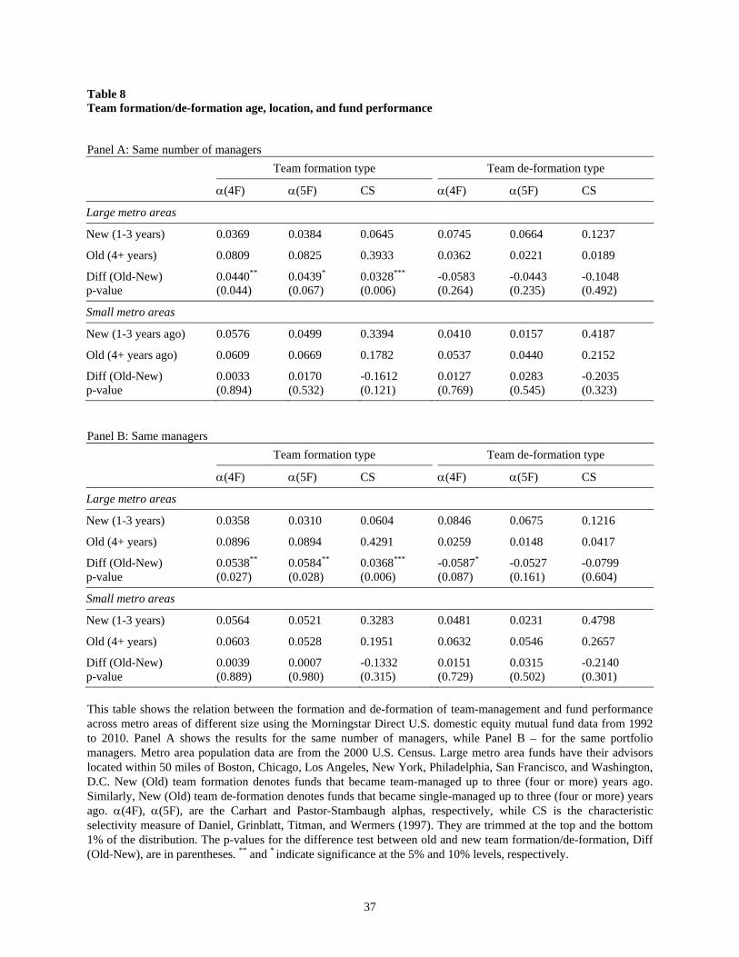
37

Table 8 Team formation/de-formation age, location, and fund performance Panel A: Same number of managers

Team formation type Team de-formation type

(4F) (5F) CS (4F) (5F) CS

Large metro areas

New (1-3 years) 0.0369 0.0384 0.0645 0.0745 0.0664 0.1237

Old (4+ years) 0.0809 0.0825 0.3933 0.0362 0.0221 0.0189

Diff (Old-New) 0.0440** 0.0439* 0.0328*** -0.0583 -0.0443 -0.1048 p-value (0.044) (0.067) (0.006) (0.264) (0.235) (0.492)

Small metro areas

New (1-3 years ago) 0.0576 0.0499 0.3394 0.0410 0.0157 0.4187

Old (4+ years ago) 0.0609 0.0669 0.1782 0.0537 0.0440 0.2152

Diff (Old-New) 0.0033 0.0170 -0.1612 0.0127 0.0283 -0.2035 p-value (0.894) (0.532) (0.121) (0.769) (0.545) (0.323)

Panel B: Same managers

Team formation type Team de-formation type

(4F) (5F) CS (4F) (5F) CS

Large metro areas

New (1-3 years) 0.0358 0.0310 0.0604 0.0846 0.0675 0.1216

Old (4+ years) 0.0896 0.0894 0.4291 0.0259 0.0148 0.0417

Diff (Old-New) 0.0538** 0.0584** 0.0368*** -0.0587* -0.0527 -0.0799 p-value (0.027) (0.028) (0.006) (0.087) (0.161) (0.604)

Small metro areas

New (1-3 years) 0.0564 0.0521 0.3283 0.0481 0.0231 0.4798

Old (4+ years) 0.0603 0.0528 0.1951 0.0632 0.0546 0.2657

Diff (Old-New) 0.0039 0.0007 -0.1332 0.0151 0.0315 -0.2140 p-value (0.889) (0.980) (0.315) (0.729) (0.502) (0.301)

This table shows the relation between the formation and de-formation of team-management and fund performance across metro areas of different size using the Morningstar Direct U.S. domestic equity mutual fund data from 1992 to 2010. Panel A shows the results for the same number of managers, while Panel B – for the same portfolio managers. Metro area population data are from the 2000 U.S. Census. Large metro area funds have their advisors located within 50 miles of Boston, Chicago, Los Angeles, New York, Philadelphia, San Francisco, and Washington, D.C. New (Old) team formation denotes funds that became team-managed up to three (four or more) years ago. Similarly, New (Old) team de-formation denotes funds that became single-managed up to three (four or more) years ago. (4F), (5F), are the Carhart and Pastor-Stambaugh alphas, respectively, while CS is the characteristic selectivity measure of Daniel, Grinblatt, Titman, and Wermers (1997). They are trimmed at the top and the bottom 1% of the distribution. The p-values for the difference test between old and new team formation/de-formation, Diff (Old-New), are in parentheses. ** and * indicate significance at the 5% and 10% levels, respectively.

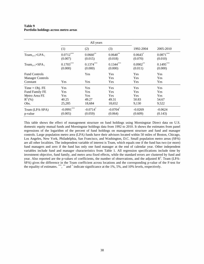
38

Table 9 Portfolio holdings across metro areas

All years

(1) (2) (3) 1992-2004 2005-2010

Teami,t-1×LPA i 0.0712*** 0.0660** 0.0640** 0.0643* 0.0871*** (0.007) (0.015) (0.018) (0.070) (0.010)

Teami,t-1×SPA i 0.1703*** 0.1374*** 0.1344*** 0.0902** 0.1495*** (0.000) (0.000) (0.000) (0.011) (0.000)

Fund Controls Yes Yes Yes Yes Manager Controls Yes Yes Yes Constant Yes Yes Yes Yes Yes

Time × Obj. FE Yes Yes Yes Yes Yes Fund Family FE Yes Yes Yes Yes Yes Metro Area FE Yes Yes Yes Yes Yes R2 (%) 40.25 49.27 49.31 50.83 54.67 Obs. 25,285 18,684 18,652 9,130 9,522

Team (LPA-SPA) -0.0991*** -0.0714* -0.0704* -0.0269 -0.0624 p-value (0.005) (0.059) (0.064) (0.609) (0.143)

This table shows the effect of management structure on fund holdings using Morningstar Direct data on U.S. domestic equity mutual funds and Morningstar holdings data from 1992 to 2010. It shows the estimates from panel regressions of the logarithm of the percent of fund holdings on management structure and fund and manager controls. Large population metro area (LPA) funds have their advisors located within 50 miles of Boston, Chicago, Los Angeles, New York, Philadelphia, San Francisco, and Washington, D.C. Small population metro areas (SPA) are all other localities. The independent variable of interest is Team, which equals one if the fund has two (or more) fund managers and zero if the fund has only one fund manager at the end of calendar year. Other independent variables include fund and manager characteristics from Table 1. All regression specifications include time by investment objective, fund family, and metro area fixed effects, while the standard errors are clustered by fund and year. Also reported are the p-values of coefficients, the number of observations, and the adjusted R2. Team (LPA-SPA) gives the difference in the Team coefficient across locations and the corresponding p-value of the F-test for the equality of estimates. ***, ** and * indicate significance at the 1%, 5%, and 10% levels, respectively.

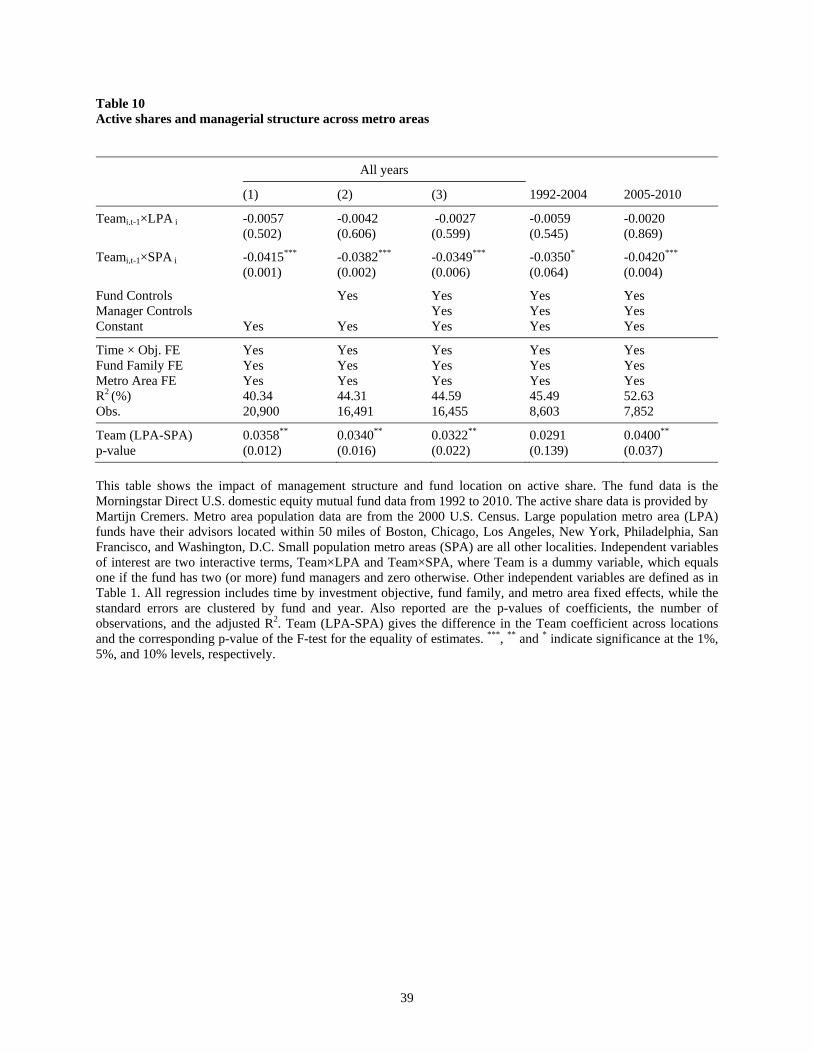
39

Table 10 Active shares and managerial structure across metro areas

All years

(1) (2) (3) 1992-2004 2005-2010

Teami,t-1×LPA i -0.0057 -0.0042 -0.0027 -0.0059 -0.0020 (0.502) (0.606) (0.599) (0.545) (0.869)

Teami,t-1×SPA i -0.0415*** -0.0382*** -0.0349*** -0.0350* -0.0420*** (0.001) (0.002) (0.006) (0.064) (0.004)

Fund Controls Yes Yes Yes Yes Manager Controls Yes Yes Yes Constant Yes Yes Yes Yes Yes

Time × Obj. FE Yes Yes Yes Yes Yes Fund Family FE Yes Yes Yes Yes Yes Metro Area FE Yes Yes Yes Yes Yes R2 (%) 40.34 44.31 44.59 45.49 52.63 Obs. 20,900 16,491 16,455 8,603 7,852

Team (LPA-SPA) 0.0358** 0.0340** 0.0322** 0.0291 0.0400** p-value (0.012) (0.016) (0.022) (0.139) (0.037)

This table shows the impact of management structure and fund location on active share. The fund data is the Morningstar Direct U.S. domestic equity mutual fund data from 1992 to 2010. The active share data is provided by Martijn Cremers. Metro area population data are from the 2000 U.S. Census. Large population metro area (LPA) funds have their advisors located within 50 miles of Boston, Chicago, Los Angeles, New York, Philadelphia, San Francisco, and Washington, D.C. Small population metro areas (SPA) are all other localities. Independent variables of interest are two interactive terms, Team×LPA and Team×SPA, where Team is a dummy variable, which equals one if the fund has two (or more) fund managers and zero otherwise. Other independent variables are defined as in Table 1. All regression includes time by investment objective, fund family, and metro area fixed effects, while the standard errors are clustered by fund and year. Also reported are the p-values of coefficients, the number of observations, and the adjusted R2. Team (LPA-SPA) gives the difference in the Team coefficient across locations and the corresponding p-value of the F-test for the equality of estimates. ***, ** and * indicate significance at the 1%, 5%, and 10% levels, respectively.

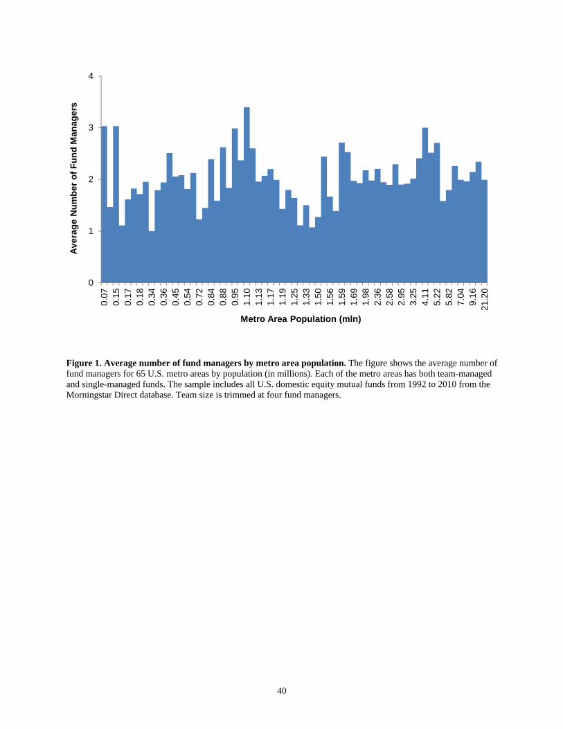
40

Figure 1. Average number of fund managers by metro area population. The figure shows the average number of fund managers for 65 U.S. metro areas by population (in millions). Each of the metro areas has both team-managed and single-managed funds. The sample includes all U.S. domestic equity mutual funds from 1992 to 2010 from the Morningstar Direct database. Team size is trimmed at four fund managers.

0

1

2

3

4

0.07

0.15

0.17

0.18

0.34

0.36

0.45

0.54

0.72

0.84

0.88

0.95

1.10

1.13

1.17

1.19

1.25

1.33

1.50

1.56

1.59

1.69

1.98

2.36

2.58

2.95

3.25

4.11

5.22

5.82

7.04

9.16

21.2

0

Av

erag

e N

um

ber

of

Fu

nd

Man

ager

s

Metro Area Population (mln)

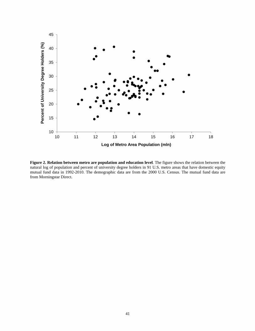
41

Figure 2. Relation between metro are population and education level. The figure shows the relation between the natural log of population and percent of university degree holders in 91 U.S. metro areas that have domestic equity mutual fund data in 1992-2010. The demographic data are from the 2000 U.S. Census. The mutual fund data are from Morningstar Direct.

10

15

20

25

30

35

40

45

10 11 12 13 14 15 16 17 18

Per

cen

t o

f U

niv

ersi

ty D

egre

e H

old

ers

(%)

Log of Metro Area Population (mln)

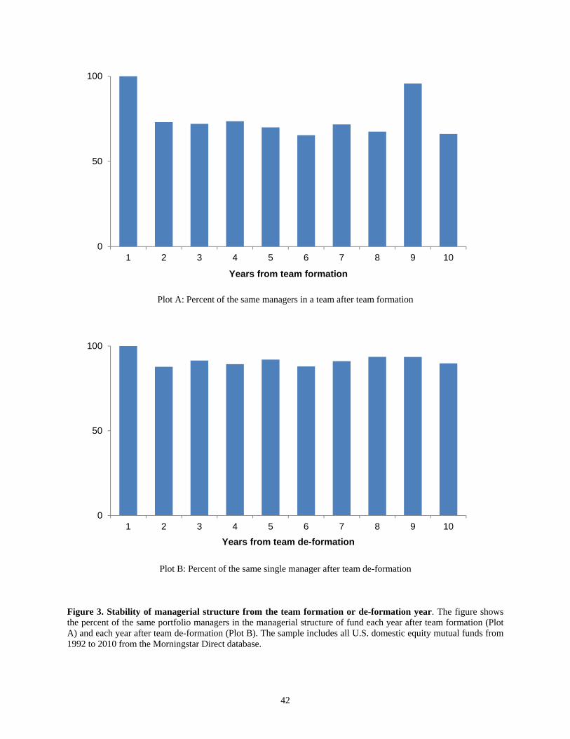
42

Plot A: Percent of the same managers in a team after team formation

Plot B: Percent of the same single manager after team de-formation

Figure 3. Stability of managerial structure from the team formation or de-formation year. The figure shows the percent of the same portfolio managers in the managerial structure of fund each year after team formation (Plot A) and each year after team de-formation (Plot B). The sample includes all U.S. domestic equity mutual funds from 1992 to 2010 from the Morningstar Direct database.

0

50

100

1 2 3 4 5 6 7 8 9 10

Years from team formation

0

50

100

1 2 3 4 5 6 7 8 9 10

Years from team de-formation

Teams, Location, and Productivity · Teams, Location, and Productivity ... The motivation for this...

Documents

Transcript of Teams, Location, and Productivity · Teams, Location, and Productivity ... The motivation for this...