Team #286 All Aboard: Can High Speed Rail Get Back on Track?

Team #286

All Aboard: Can High Speed Rail Get Back on Track?

166

166Copyright © SIAM Unauthorized reproduction of this article is prohibited

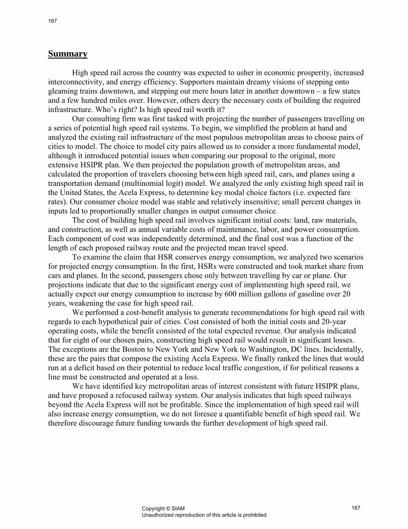
Summary High speed rail across the country was expected to usher in economic prosperity, increased interconnectivity, and energy efficiency. Supporters maintain dreamy visions of stepping onto gleaming trains downtown, and stepping out mere hours later in another downtown – a few states and a few hundred miles over. However, others decry the necessary costs of building the required infrastructure. Who’s right? Is high speed rail worth it? Our consulting firm was first tasked with projecting the number of passengers travelling on a series of potential high speed rail systems. To begin, we simplified the problem at hand and analyzed the existing rail infrastructure of the most populous metropolitan areas to choose pairs of cities to model. The choice to model city pairs allowed us to consider a more fundamental model, although it introduced potential issues when comparing our proposal to the original, more extensive HSIPR plan. We then projected the population growth of metropolitan areas, and calculated the proportion of travelers choosing between high speed rail, cars, and planes using a transportation demand (multinomial logit) model. We analyzed the only existing high speed rail in the United States, the Acela Express, to determine key modal choice factors (i.e. expected fare rates). Our consumer choice model was stable and relatively insensitive; small percent changes in inputs led to proportionally smaller changes in output consumer choice. The cost of building high speed rail involves significant initial costs: land, raw materials, and construction, as well as annual variable costs of maintenance, labor, and power consumption. Each component of cost was independently determined, and the final cost was a function of the length of each proposed railway route and the projected mean travel speed.

To examine the claim that HSR conserves energy consumption, we analyzed two scenarios for projected energy consumption. In the first, HSRs were constructed and took market share from cars and planes. In the second, passengers chose only between travelling by car or plane. Our projections indicate that due to the significant energy cost of implementing high speed rail, we actually expect our energy consumption to increase by 600 million gallons of gasoline over 20 years, weakening the case for high speed rail.

We performed a cost-benefit analysis to generate recommendations for high speed rail with regards to each hypothetical pair of cities. Cost consisted of both the initial costs and 20-year operating costs, while the benefit consisted of the total expected revenue. Our analysis indicated that for eight of our chosen pairs, constructing high speed rail would result in significant losses. The exceptions are the Boston to New York and New York to Washington, DC lines. Incidentally, these are the pairs that compose the existing Acela Express. We finally ranked the lines that would run at a deficit based on their potential to reduce local traffic congestion, if for political reasons a line must be constructed and operated at a loss.

We have identified key metropolitan areas of interest consistent with future HSIPR plans, and have proposed a refocused railway system. Our analysis indicates that high speed railways beyond the Acela Express will not be profitable. Since the implementation of high speed rail will also increase energy consumption, we do not foresee a quantifiable benefit of high speed rail. We therefore discourage future funding towards the further development of high speed rail.

167


Table of Contents Summary ............................................................................................................................................ 167

Introduction ........................................................................................................................................ 169Background ................................................................................................................................ 169Restatement of the Problem ....................................................................................................... 169Global Assumptions ................................................................................................................... 169

Part I: Forecasting Ridership ............................................................................................................. 169Analysis of Cost and Time ......................................................................................................... 170Car Travel Cost and Time .......................................................................................................... 170Plane Travel Cost and Time ....................................................................................................... 170High Speed Rail Travel Cost and Time .....................................................................................171

Total Trips Between Cities ........................................................................................................ 172Number of Intercity Travelers per Year..................................................................................... 172City Population Through 2032................................................................................................... 172Analysis of Traveler Preference................................................................................................. 172

Sensitivity Analysis ...................................................................................................................173Part II: Initial Costs of High Speed Rail .......................................................................................... 175

Land Ownership Cost .............................................................................................................. 175

Facility Development Cost ...................................................................................................... 175Railroad Track Cost ................................................................................................................. 176Train Cost................................................................................................................................. 176

Part III: Variable Costs Model ......................................................................................................... 177Facility Upkeep Cost................................................................................................................ 177Labor Cost ................................................................................................................................ 177Power Cost ............................................................................................................................... 178Consolidated Total Cost ........................................................................................................... 178

Part IV: High Speed Rail and Energy Consumption .......................................................................180

Part V: Prioritization of HSR Construction ..................................................................................... 181Part VI: Sensitivity Analysis ............................................................................................................ 184Conclusion ....................................................................................................................................... 184Bibliography .................................................................................................................................... 185Appendix A ...................................................................................................................................... 186

168


Introduction

Background A symbol of technological prowess and everyday luxury, high speed rail (HSR) has revolutionized public transportation in Europe and Asia. First developed by Japan in 1964, HSR systems have grown wildly in popularity in the past two decades [1]. Today, China has the world’s largest HSR system, with over 3,700 miles of track, while the European Union has planned a Trans-European High Speed Rail System [2]. The United States, in contrast, has only one HSR line: the Acela Express, privately owned by Amtrak, which spans less than 500 miles [3]. The Obama administration is encouraging the development of a nationwide system of high-speed rail lines, stating that it would ease traffic, alleviate transportation pressure on the environment, and boost the economy. States have caught on to the idea of high speed rail, submitting almost 300 preliminary proposals, requesting a total of $102 billion in federal funding [4].

While some state and federal departments agree that the construction of high speed rail makes sense, Congress rejected HSIPR funding last November because it was perceived to be fiscally unsound. While the Acela Express has turned a profit of about $41 dollars per passenger, concerns remain about the significant amount of government subsidies sought and the stated potential for employment and profit.

Restatement of the Problem Our consulting firm was asked to:

1. Identify metropolitan regions of particular interest in developing high speed rail infrastructure and service.

2. Analyze current ridership of HSR and forecast future consumer choice of transportation modes over the course of 20 years.

3. Analyze the sensitivity of the ridership forecasts to parameters used, with particular focus on travel times.

4. Determine cost estimates for the initial construction of high speed rail and future maintenance costs.

5. Analyze any possible effect of the prevalence of high-speed rail on foreign energy dependence.

6. Rank the ten HSIPR-identified regions based on the results of the previous models.

Global Assumptions 1. We will assume a steady state of foreign and political affairs in the nation. Potential supply

shocks or future economic catastrophes will be ignored in these models. 2. High speed rail systems will be constructed alongside conventional tracks to minimize

costs. 3. Because public and governmental support for HSR is liable to change, the model will not

consider potential subsidies or political opposition. 4. The same HSR technology will be used across the United States.

Part I: Forecasting Ridership In our model, we generate a new, refocused proposal for constructing High Speed Rail focused between pairs of major metropolitan areas. We disregarded commuters within one metropolitan area because, at such small distances, travel by car dominates over travel by High

169


Speed Rail [5]. In addition, trips of distances greater than several hundred miles will be dominated by air travel [6]. Thus, High Speed Rail travel is only relevant for cities in the same geographic region, at least 100 miles apart.

To choose which pairs of metropolitan areas to analyze, we examined the most populated cities in each geographic region of the United States and overlaid that with a map of existing railway infrastructure. We chose pairs of cities that were at least 100 miles away from each other, with currently extant track and railway stations. The pairs of cities corresponded roughly with the ten proposed HSIPR regions, but with much narrower itineraries. The pairs include Miami and Tampa; Chicago and St. Louis; San Francisco and Los Angeles; Dallas and Houston; Detroit and Chicago; Boston and New York City; Seattle and Portland; Washington, D.C. and New York; Philadelphia and Pittsburgh; and Houston and Atlanta.

Analysis of Cost and Time Assumptions

Since there is no clear trend in gasoline prices, the price of gasoline will be assumed constant for the model at this time.

The population’s income increases with inflation. Therefore, the relative disutility (cost) of traveling by train, car, or plane will remain constant for the future. Travel cost will be calculated in current dollars.

Since the timeframe is relatively short, plane fares and prices will be assumed constant. HSR fares nationwide will follow distance trends seen in the existing Acela Express data,

scaling with distance traveled. This is reasonable because currently, fares are calculated by different “zones”: fares increase with the distance traveled.

Car Travel Cost and Time The primary costs of an individual travelling by car are the price of fuel, and the

opportunity cost of time spent driving. The national average cost for fuel per gallon in 2010 was $3.60 [7]. The average mileage of a passenger car in 2010 was 23.8 mpg [8].

Thus, the expected cost ( ) for a car ride of a distance of miles is:

The road distances and times required for car rides between the ten pairs of cities were found using Google Maps, taking into account the traffic on highways on Monday at 7:45 AM – a reasonable time for business travelers or day trips. Plane Travel Cost and Time

Plane travel becomes relevant for longer trips due to its higher speed. Prices for nonstop flights between the ten major pairs of cities were found by checking Travelocity for flight fare and on Monday, April 9, 2012, departing at approximately 7:00 AM. This time was chosen because it is representative of typical business travel conditions, a Monday morning that does not follow any major holidays. The date is also several weeks in the future, avoiding the increase in price that typically leads up to a flight’s date.

Specific prices were used, rather than modeling the price in general, because the price for an airplane ticket depends on many factors apart from distance traveled, including competition along the route and airline connectivity.

170


60 minutes were added to flight duration to account for time spent in security (20 minutes on average), takeoff, and docking, assumed 20 minutes each [9].

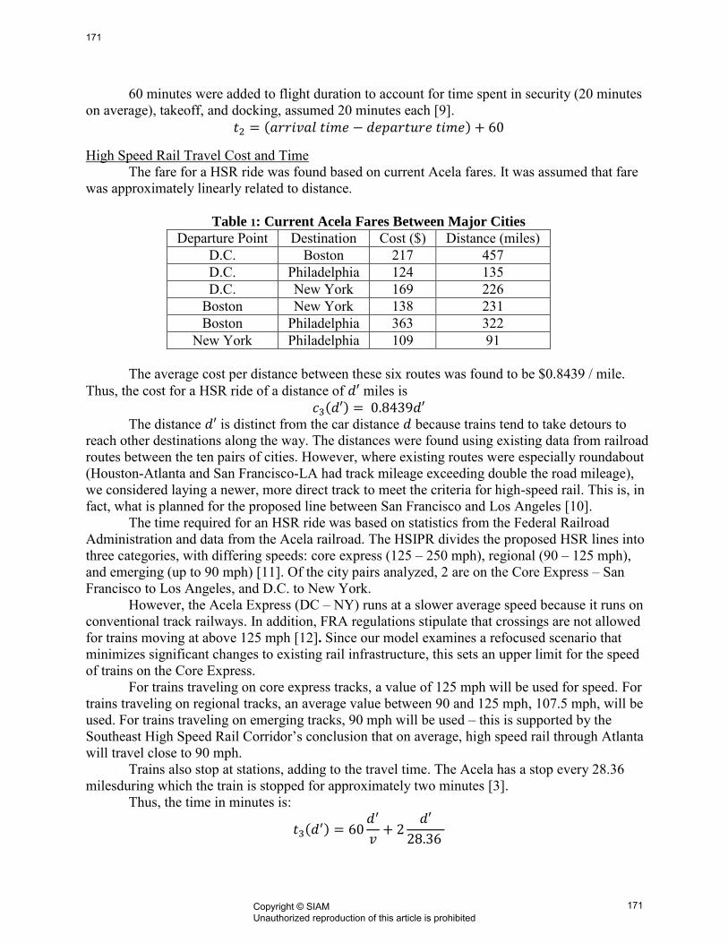
High Speed Rail Travel Cost and Time The fare for a HSR ride was found based on current Acela fares. It was assumed that fare

was approximately linearly related to distance.

Table 1: Current Acela Fares Between Major Cities

Departure Point Destination Cost ($) Distance (miles) D.C. Boston 217 457 D.C. Philadelphia 124 135 D.C. New York 169 226

Boston New York 138 231 Boston Philadelphia 363 322

New York Philadelphia 109 91

The average cost per distance between these six routes was found to be $0.8439 / mile. Thus, the cost for a HSR ride of a distance of miles is

The distance is distinct from the car distance because trains tend to take detours to reach other destinations along the way. The distances were found using existing data from railroad routes between the ten pairs of cities. However, where existing routes were especially roundabout (Houston-Atlanta and San Francisco-LA had track mileage exceeding double the road mileage), we considered laying a newer, more direct track to meet the criteria for high-speed rail. This is, in fact, what is planned for the proposed line between San Francisco and Los Angeles [10]. The time required for an HSR ride was based on statistics from the Federal Railroad Administration and data from the Acela railroad. The HSIPR divides the proposed HSR lines into three categories, with differing speeds: core express (125 – 250 mph), regional (90 – 125 mph), and emerging (up to 90 mph) [11]. Of the city pairs analyzed, 2 are on the Core Express – San Francisco to Los Angeles, and D.C. to New York. However, the Acela Express (DC – NY) runs at a slower average speed because it runs on conventional track railways. In addition, FRA regulations stipulate that crossings are not allowed for trains moving at above 125 mph [12]. Since our model examines a refocused scenario that minimizes significant changes to existing rail infrastructure, this sets an upper limit for the speed of trains on the Core Express. For trains traveling on core express tracks, a value of 125 mph will be used for speed. For trains traveling on regional tracks, an average value between 90 and 125 mph, 107.5 mph, will be used. For trains traveling on emerging tracks, 90 mph will be used – this is supported by the Southeast High Speed Rail Corridor’s conclusion that on average, high speed rail through Atlanta will travel close to 90 mph. Trains also stop at stations, adding to the travel time. The Acela has a stop every 28.36 milesduring which the train is stopped for approximately two minutes [3].

Thus, the time in minutes is:

171


Total Trips Between Cities Assumptions

1. Cities in the United States have uniform “pull”, not attracting significantly more travelers per person than any other cities in the United States.

2. Consumers traveling distances of approximately 2-5 hours (by car) will choose between driving, flying, or taking HSR.

3. The growth/decline pattern of residents in metropolitan areas between 2000 and 2005 is representative of the growth/decline rates through 2032.

4. The personal preferences of citizens in the 20 selected cities towards HSR, plane, or car travel are distributed similarly to those of citizens in the Boston and New York City (this affects the value of in the multinomial regression).

5. The amount of trips per year between any two cities per year is proportional to the amount of trade between them.

6. The“economic mass” of cities is proportional to the population of each city.

Number of Intercity Travelers per Year According to the Gravity Model of Trade, the amount of trade between two nations is

proportional to the product of their economic masses and is inversely proportional to the distance between them [13], [14]. With the assumptions,

where is the number of trips between two cities per year, the are the populations, and is the distance between the cities in miles. The proportionality constant was found from data between Boston and New York City. The total number of Acela tickets sold between these two cities in the 2010 fiscal year was 593,300, with Acela taking a 27% market share [15]. According to the 2010 Census, the. The population of the greater Boston metropolitan area in 2010 was 3,975,317 and the population of the greater New York City metropolitan area in 2010 was 20,426,870, with the distance between them equal to 218 miles.

City Population Through 2032

Because the growth rate of metropolitan areas over time is variable, the population of such areas will be modeled using a logarithmic curve determined by the 6 year data estimates from 2000 to 2005. The U.S. Census Bureau used the 2005 data to estimate the population of the metropolitan area for each of the 5 previous years. We chose a logarithmic curve because these metropolitan areas are approaching a “carrying capacity”, where growth is limited by space and economic constraints [16].

The 6 year data was plotted on a graph and the best-fit logarithmic curve was found as a function of number of years after 2000. The resulting equation was then applied from the 2012 (year 12) to 2032 (year 32), resulting in the annual population of each metropolitan area.

The full population projections are shown in Appendix A.

Analysis of Traveler Preference The proportion of travelers who decide to take the HSR, as opposed to a plane or car, will be modeled using a multinomial logistic regression. The independent variables are cost (in dollars), and time required (in minutes), and the dependent variable is the choice of transportation (plane,

172


car, or HSR). We define the disutility function (a measure of the total cost) for a transportation method as

According to the logistic regression, the proportion of travelers who choose method , , is equal to

where the minus signs are added because the are disabilities rather than utilities. Since is a scaling factor, only the ratio of and is important. Without loss of generality, set equal to 1/60. The value of can be found through opportunity cost. The average hourly wage of an American worker, in 2011, was $23.25 [7]. Then the disutility of spending 60 minutes commuting is equal to the disutility of spending $23.25 commuting:

The value of is found using the precedent set by Acela. In 2010, Acela took a 27% market share of all intercity traffic between Boston and New York City [15]. Plugging in the known values,

We now apply the regression to all ten pairs of cities.

Table 2: Projected Annual Ridership for Cars, Planes, and HSR in 2012

City Pair Car Plane HSR Tampa and Miami 135,083 144,460 93,834

Chicago and St. Louis 208,311 218,775 148,083 San Francisco and Los Angeles 267,472 334,652 175,823

Dallas and Houston 291,536 318,347 215,170 Detroit and Chicago 259,993 319,618 187,607

Boston and New York City 749,290 817,176 562,504 Seattle and Portland 19,990 19,749 16,315 D.C. and New York 1,044,909 1,071,000 787,252

Philadelphia and Pittsburgh 96,798 51,336 66,926 Houston to Atlanta 56,955 86,172 20,575

Combining this with the data on trips made between pairs of city each year found through the gravity model, the ridership for each city pair was found in the year 2012, for cars, planes, and HSR (results for other years are omitted for brevity). The annual ridership was also generated for all years up to 2032, without including HSR as a possibility. This will be used to compare the effect on emissions by adding HSR in the next section. The data for 2012 is displayed in Appendix A.

Sensitivity Analysis We examined the sensitivity of our multinomial logit model of consumer choice to travel time and ticket fare. We changed travel time by +/- 2, 4, and 10% and examined the resulting change in proportion of high-speed rail users, the output of the logit model. For simplicity, we only examined the changes for one pair of cities, Miami to Tampa. We repeated the same process for analyzing sensitivity of fare prices.

173


y = 0.1265x -0.015

0

0.015

-0.15 0.00 0.15

Re

sult

ing

pe

rce

nt

de

cre

ase

s in

pro

po

rtio

n H

SR

Percent decreases in fare

Figure 1: Resulting percent decreases in proportion of consumers choosing

high speed rail vs. percent changes in travel time

Figure 2: Resulting percent changes in proportion of consumers choosing high speed rail vs. percent changes in fare price

The proportion of HSR travelers responds approximately linearly to small relative changes

in travel time and fare, with slopes of 0.042 and 0.126 respectively. Since the coefficient for fare cost was approximately three times the coefficient for time, the sensitivity analysis shows that the conclusions are self consistent. In addition, since the slopes are relatively small, a small error in the initial parameters would not significantly change the output of the model. Testing the Model The logarithmic population model can be tested by running it backwards and using past Census data to check the validity of the numbers, in 1990, 1980, etc.. The gravity model can be tested by summing the expected number of trips over every pair of major cities in the United States and compare this to the actual total number of trips taken. Since Americans make a total of about 405 million long distance business trips per year and about an equal amount of leisure trips, the total number of trips should be approximately 810 million [17].

y = 0.0427x -0.015

0

0.015

-0.15 0.00 0.15

Re

sult

ing

pe

rce

nt

de

cre

ase

in

pro

po

rtio

n o

f H

SR

Percent decrease in travel time

174


The multinomial logistic regression model can be tested by removing the High Speed Rail option. This leaves only the existing options: car, plane travel, and conventional rail. The results can be compared against actual results for 2012 and previous years.

Part II: Initial Costs of High Speed Rail In order to determine the costs associated with the development and maintenance of high speed rail systems, two separate models were created and evaluated. The first model considers the one-time costs incurred in order to construct the necessary infrastructure, while the second model investigates the cost of upkeep with time. The basis for the initial cost model is as follows:

The total one-time cost ( of high speed rail is a function of the cost of land ownership

rights ( , the costs of developing initial servicing and maintenance stations along the tracks ( , the cost of physically constructing the steel railroad track ( , and the cost of the trains themselves ( ). Each component of the one-time cost is a function of the length of the railroad tracks between the two locations connected by the high speed rail system .

Land Ownership Cost Assumptions

1. The cost for purchasing an easement on which to construct a railroad track remains constant for the duration and length of the construction.

2. A first-order assumption made by the model is that regional variability for the cost of land ownership is not a significant factor. This assumption, made to simplify our analysis given certain time constraints, is potentially problematic and should be the one of the first to be addressed in further iterations.

3. Due to lower long term cost for the railroad company, the decision to purchase rather than rent the easement will be chosen by the company.

The land ownership is determined by first finding the cost per mile for an easement. The

values for easement throughout the country are averaged to find a nation-wide average for the easement. This value was determined to be $45,000 per mile [18]. Then, the land ownership cost is determined as a function of total railroad track length by multiplying easement value of $45,000 per mile by the total length of the potential railroad. This determines the total cost for land purchases by the railroad company, W(x):

Facility Development Cost Assumptions

1. The railroad company will use existing railroad stations for the high-speed railways to save money on development of required facilities.

2. The distribution of maintenance facilities will be uniform along the constructed railroad track.

We must determine the number of maintenance stations required to calculate maintenance

costs of facilities. Based on FRA regulations, buildings that store equipment and materials necessary for train and rail maintenance are required every 50 miles along the track. To meet the FRA regulations, we round up the number of stations calculated for each route [19].

175


We analyze the costs of constructing maintenance facilities on the Western North Carolina Railroad (WNCRR) and in Texas and calculate a cost of $375,000 per facility [20]. Multiplying the cost per facility with the total number of required facilities for the railway track results in the final equation for facility cost:

Railroad Track Cost Assumptions

1. The composition and cross sectional volume of railroad tracks remains constant for the length of the railway.

2. The cost of steel, concrete, gravel, and crushed stone will remain constant for the duration of construction of the railway.

We find the volume of each material (per the cross-sectional area of track) to find the total

material cost of building the track itself. As seen in Figure 3, the cross section of a railroad track includes the rail and fastenings (consolidated into the rail), the sleeper, the ballastbed, and the sub-ballast. Figure 3: Cross Sectional Area of Railroad Track (Omitted due to copyright concerns: image portrays the cross-section,

which includes subgrade, sub-ballast, ballastbed, rail, sleeper, and fastening)

The cross sectional area is determined by the depth and width of each section. The cross section of rail and fastening (Rail) is composed of steel, the cross section of the sleeper (Sleeper) is composed of concrete, the cross section of the ballastbed (Ballastbed) is made of crushed stone, and the cross section of the sub-ballast (Subballast) of gravel [21]. The sleeper is only present every 0.6 meters (0.000373 miles). The cost per weight of steel (S), concrete (Co), crushed stone (Cs), and gravel (G) are multiplied by their respective densities (ρS, ρCo, ρCs, ρG) to arrive at the cost per volume of each material [22]. The product of the cost per volume, cross sectional area, and variable length of the railroad track result in the total cost necessary for the railroad track. The total cost of the railroad track is given by:

Train Cost Assumptions

1. Amtrak purchased the trains used in the Amtrak Acela Express at a market rate that remains constant for all railroad companies.

2. Train sets purchased from different companies cost approximately the same. 3. The number of required trains necessary to maintain periodic trips between stations on the

railway is proportional to the total length of track by a train density ratio (K). Although these high speed rails will run alongside extant track, more track must be laid

down for safety and regulatory issues. More trains will be necessary to maintain periodic trips along the track throughout each day than for conventional rail. Thus, existing data for the Amtrak Acela Express railway is used to estimate the total number of trains required by the potential railway routes [3]. We determine a high speed rail “train density ratio” of 0.0609 trains per mile of track [23]. The individual train cost was then determined from the cost Amtrak paid for 20 train sets when developing the Amtrak Acela Express railway. The train sets of 8 cars each were purchased at 20 sets for $600 million from companies in Quebec and France, or $30 million per train set.

176


The final train cost is a function of the total track distance, the train density ratio, and the cost per individual train set.

Part III: Variable Costs Model

The annual variable costs ( ) of high speed rail are dependent on the cost of facility upkeep ( ), the cost of a functioning labor force ( ), and the cost of the power necessary to keep the train serviceable ( ). The facility upkeep and labor costs are directly a function of the length of track that separates the two major endpoint stations, while the annual power usage is a function of the train density ratio, the length of track, and the average velocity of the high speed train along its path ( , respectively).

Facility Upkeep Cost Assumptions

1. The only costs incurred will be those of traditional maintenance and facility operating costs. The cost of facility upkeep can be found by taking the product of the number of

maintenance and service facilities and the expected cost of annual servicing. The ceiling function serves the same function as it did in the Facility Development Cost Model: determining the expected number of service stations along a given length of track. The cost of annual servicing is $324,000 per year per station [20]. To find total upkeep cost, we multiplied that annual servicing charge by the total number of servicing stations along the railroad track. In the following equation, the ceiling function gives the least integer that is greater than or equal to x/50, or the total mileage of track divided by 50.

Labor Cost Assumptions

1. The available data from Metrorail is representative of that of other railroad companies, including Amtrak.

The cost of hiring employees to work at each station along the railroad is integral to

maintenance. The data available on the distribution and average salary of workers at Metrorail are used to approximate the distribution of workers along similar stations in a high-speed railway.

The jobs present at stations built along the rail are distributed into train operators, station managers, police, train operations managers, technicians, police, railcar cleaners, and station janitors (Metrorail). The data for the necessary number of each type of job are divided by the total number of existing stations, which determines the average number of workers per station. The number of worker at each station is multiplied by the average cost for that type of worker. The individual costs for each job type are summed to derive the total labor cost per station of $1,333,974.42.

The value for the number of stations along the railroad track originally determined in the facility development cost model is then multiplied by the aforementioned value of labor cost per station to arrive at the total cost for a specific length of constructed high-speed railway track.

177


Power Cost Assumptions

1. The high speed rail system will be powered by rail electrification as opposed to diesel engines given the industry-wide preference for electric power due to its better power to weight ratio and accelerative capabilities.

2. The power consumption of the Amtrak Acela Express is representative of the power consumption of the prospective high speed rail systems given US standards for voltage and frequency.

3. The price of power consumption per kilowatt-hour for the high speed rail systems is equal than or less to the price of residential power consumption given the orders of magnitude difference in aggregate usage.

4. On average, trains will run once a day. Trains that may run more than once in a day will be effectively cancelled out by those trains that do not run that day.

The power cost for one year is determined through an understanding of power

consumption of an electrified high-speed rail in kilowatts, price of the power consumption per unit time, and the total duration of rail travel during the year. The expected power consumption of a high-speed rail is 9,200 kW [8]. The price for that amount of power is $0.12 per kW-hr, the use of 1 kW of power for 1 hour [24].

The parameters of the power model are divided up into Kx and x/v. The number of trips made each day is represented by Kx, where K is the train density ratio the value of Kx is the total expected number of trips made each day on a regular schedule. The value of x/v is equal to the total time of the trip and power is assumed to be constant with regards to time. The value of Kx2/v is equal to the total duration of rail travel per day, which is then multiplied by 365 to determine the annual duration. The total power is then found by multiplying the value by the previously determined cost of power per time, $1,104 per hour.

Consolidated Total Cost

The final cost given by these initial and variable cost models:

where x, the distance of the potential railway, and v, the average train speeds along the railway, are plugged into the equations. The distance and speed for the railway for the 10 pairs of major city originally defined in Part I are input into the cost model and the final cost is shown in

178


Table 3.

179


Table 3: Final Initial and Variable Costs for Inter-city Railways

Length in miles (x)

Speed in mph (v) Initial Cost Variable Cost

Tampa and Miami 277.2 90 $551,644,489 $30,899,735 Chicago and St. Louis 282 107.5 $561,157,813 $28,101,707 San Francisco and LA 381 125 $758,120,131 $41,762,109

Dallas and Houston 241 90 $479,523,167 $24,126,795 Detroit and Chicago 281 107.5 $559,175,871 $27,973,184

Boston and New York City 231 73 $459,703,741 $26,228,133 Seattle and Portland 467 107.5 $929,317,194 $66,365,434 D.C. and New York 226 73 $449,794,028 $25,459,989

Philadelphia and Pittsburgh 353 90 $702,625,738 $47,240,882 Houston and Atlanta 793 90 $1,577,680,482 $197,995,596

Part IV: High Speed Rail and Energy Consumption About 49% of the petroleum consumed by the US originated from foreign countries in

2010, and 42% of that oil originates from OPEC countries (EIA). Our oil supply is therefore extremely vulnerable to supply shocks and political instability, as seen during the Gulf War and the recent revolts in Libya and Egypt. As recently as January 9, Iran has threatened to block the Strait of Hormuz, a key shipping lane for oil [25]. Even discounting political factors, it is estimated that the global petroleum supply will be depleted in 41 years [26].

Proponents of high-speed rail claim that since HSR uses less energy per passenger-mile, significant amounts of oil will be conserved compared with other transportation methods. However, other conflicting analyses claim that with the energy required to construct HSR and energy losses from braking, it is actually less energy-efficient [27].

Assumptions

1. The model will assume that car, airplane, and train efficiencies, relative to each other, will not change significantly over the time period of interest.

2. Efficiency of gasoline, or its extraction from crude oil, will not change 3. On an aggregate level, the cost of constructing high speed rail scales linearly with distance.

Our model examines HSR’s effect on energy independence by comparing the energy

consumption between two scenarios: one where HSR exists and reduces car and plane passengers, and one where passengers choose between planes and cars. In the first scenario (1), we calculate the total energy consumed by passengers on high speed rail, cars, and planes. In the second scenario (2), we consider the total energy consumed by planes and car passengers.

In the second scenario, the proportions of metropolitan area populations that prefer certain modes of transportation is given by a similar binomial logit model as was used in Part 1:

180


The same values are used as in Part 1, except now the population chooses between only vehicular and aviation transport.

For HSR, there is a one-time fixed cost for construction of these new railways. The EIS estimates that it will take 150 trillion BTU to build the proposed high-speed rail system. The 2010 HSIPR plan proposed to lay 17,000 miles of high-speed rail by 2030. Our model significantly reduces the proposed length of track to 2575 miles (excluding the current track laid between Boston and New York). Therefore, the approximate energy cost of constructing our HSR model is

, or 28.3 trillion BTU.

The total energy use for the new, proposed high-speed rail system is equal to:

where the energy used in constructing HSR is equivalent to the sum of the energy required to construct HSR in our model and the HSR passenger ridership ( times times the energy efficiency of transport, (BTU/passenger-mile); summed over the relevant track mileage and rider populations (of 20 years) of each pair of cities [12]. The total energy use for cars and planes is given by:

where or is the sum of passenger (plane or car) ridership of each transportation mode each of the next 20 years. These equations remain the same between scenarios, except for the proportion of passenger ridership, given by the modified binomial logit model.

Table 4: Energy Consumption, With and Without Addition of High Speed Rail

Scenario 1 (BTU) Scenario 2 (BTU) Energy difference (BTU) Energy difference (gals) 147,706,259,880,516 73,074,623,922,234 -74,631,635,958,282 -605,721,264.856

These results suggest that with the significant energy input of actually constructing high

speed rail, the implementation of high speed rail will not actually reduce petroleum consumption at all. In fact, it will lead to an approximate increase of 600 million gallons of gasoline consumed; not a potential alleviation of foreign oil dependence by any means.

The implementation of high-speed rail will not reduce oil consumption or foreign oil dependence. If that is the goal, methods of implementing alternative fuels or exploiting domestic shale oil resources may prove more promising.

Part V: Prioritization of HSR Construction Assumptions:

1. The percentage of people who travel is constant through geographic populations.

181


2. The miles of highway in a metropolitan area is proportional to the miles of highway in its surrounding state. In order for our plans to be realistically approved by Congress, these proposed railways

must pay for themselves. Of the 44 lines that Amtrak runs across the United States, only 3 yielded a profit (subsidyscope). The losses experienced by these lines ranged from $5 to $462 dollars per passenger. The total average loss Amtrak experienced per ticket was $32 in 2008.

Acela, however, made a profit of about $41 per passenger. This indicates that there is a sustainable market for high-speed rail to substitute some existing normal rail lines. In order to determine which rail lines are effective, an analysis must be done in order to determine the expected profit for each of the ten lines.

The formula for profit is

if

t

y CtCtRP

))()(()2032(2032

2012

Expected Profit Function

whereRy is the yearly revenue, Cf is the yearly operating cost and Ci is the initial cost of construction. The most important qualification for a rail is that profit is greater than or equal to zero. The cost effectiveness of each line was calculated using this formula. If a line was determined to be cost ineffective (a net loss) then it is not suggested that that line be constructed. However, if the line is determined to be cost effective (has neutral revenue or makes a profit) then that line would be recommended for construction.

Table 5: Profit of Major Lines Over 20 Years

As indicated by

Table 5, only the Boston and New York and Washington and New York turn a profit and

completely pay off their initial construction costs. The Acela Express consists of these two lines.

Line Revenue Over 20

Years Maintenance Over

20 Years Initial Construction

Costs Profit Over 20 Years Tampa and Miami $457,126,321 $617,994,699 $551,644,488 -$712,512,866

Chicago and St. Louis $753,632,871 $562,034,131 $561,157,813 -$369,559,072 San Francisco and Los

Angeles $1,184,403,898 $835,242,189 $758,120,130 -$408,958,421 Dallas and Houston $897,051,933 $482,535,902 $479,523,166 -$65,007,135 Detroit and Chicago $908,052,945 $559,463,681 $559,175,870 -$210,586,606

Boston and New York City $2,143,041,113 $524,562,655 $459,703,740 $1,158,774,717 Seattle and Portland $49,031,266 $1,327,308,676 $929,317,194 -$2,207,594,604 D.C. and New York $3,071,264,247 $509,199,777 $449,794,027 $2,112,270,442

Philadelphia and Pittsburgh $351,860,640 $944,817,631 $702,625,737 -$1,295,582,728 Houston and Atlanta $280,965,264 $3,959,911,920 $1,577,680,481 -$5,256,627,136

182


Judging by this data alone, only two lines – the existing ones - could be fiscally justified without large ticket subsidies for each of the riders on each of the other lines.

A public good not yet quantified is the ability of high-speed rail to alleviate vehicular traffic. Although environmentally, it is optimal to remove as many cars from the road as possible, it makes more sense from a holistic transportation perspective to minimize traffic density, the ratio of cars on the road per miles of highway for a given state.

The number of motor vehicles per state passed by the railroad was taken from data provided by the U.S. Department of Transportation. This was divided by the miles of highway in the same states, using data provided by the DOT.

Highway Density =

Table 6: Highway Density by State

(Federal Highway Adminstration) However, any of the rail lines that would generate a negative income for Amtrak need to

be built because of pressing infrastructure or political needs, we should maximize the potential to minimize traffic density, DT, while minimizing debt incurred. To maximize this, we determine the ratio of traffic density to the total debt debt the line would run over 20 years. The rail line with the lowest magnitude of the ratio of total costs to DT gives the railway route with the most utility.

Table 7: Gross Profit over 20 Years by Railway Line

Rail Line Profit Over 20 Years Dt Ratio

Tampa and Miami -$712,512,866.61 9073.16 78,529.74 Chicago and St. Louis -$369,559,072.54 4127 89,546.66 San Francisco and Los Angeles -$408,958,421.55 11701.38 34,949.59 Dallas and Houston -$65,007,135.89 3228.97 20,132.47 Detroit and Chicago -$210,586,606.76 5001.63 42,103.60 Seattle and Portland -$2,207,594,604.35 6317.12 349,462.19 Philadelphia and Pittsburgh -$1,295,582,728.12 4884.21 265,259.42 Houston and Atlanta -$5,256,627,136.92 4029.76 1,304,451.66

Our analysis indicates that the Washington to New York line should be constructed first,

followed by the Boston to New York line. These two lines are the most fiscally sound. The rest of the lines would be most effective at reducing highway density, and are ranked in descending order based on their ability to do so.

Rail Line States Included Total Cars Total Miles of Highway DT

San Francisco to Los Angeles CA 30,248,069 2,585 11701.38 Tampa to Miami FL 14,526,125 1,601 9073.16

Seattle to Portland WA, OR 8,439,677 1,336 6317.12 Detroit to Chicago MI, IN, IL 23,522,687 4,703 5001.63

Philadelphia to Pittsburgh PA 9,724,453 1,991 4884.21 Washington D.C. to New York DC, MD, PA, NJ, NY 31,342,716 6,511 4813.81

Boston to New York City NY, CT, RI, MA 20,050,375 4,645 4316.55 Chicago to St. Louis IL, MO 13,709,886 3,322 4127.00 Houston to Atlanta GA, AB, MS, LA, TX 32,612,885 8,093 4029.76 Dallas to Houston TX 14,888,780 4,611 3228.97

183


These lines should be constructed after the first 2 fiscally sound lines, if overriding external needs require it, in descending order of priority: Dallas and Houston; San Francisco and Los Angeles; Detroit and Chicago; Tampa and Miami; Chicago and St. Louis; Philadelphia and Pittsburgh; Seattle and Portland; Houston and Atlanta.

Part VI: Sensitivity Analysis We now examine the sensitivity of our cost models with respect to our input parameters.

The length of track remains constant, so we focus our analysis on the impact of speed of travel on expected profitability values. Factors including rail congestion and number of passenger stops can influence average speed beyond the scope of our model. When expected speed is relatively adjusted upwards, each line shows a definite trend of decreasing variable cost. Upon testing the extreme values for new possible variable costs in the expected profit function, we determine that the decisions regarding each line’s prioritization did not change.

Figure 4: Sensitivity of Cost to Speed

Conclusion This study determined that high speed rail implementation is prohibitively expensive and would not accomplish the goals that many promise it would – namely, decreasing transportation costs and reducing foreign oil consumption. Based on the characteristics of high-speed rail and existing rail infrastructure, key areas of interest were identified. We determined the proportion of intercity travelers who would ride the proposed HSR system and the total revenue of each line, based on population projections for these metropolitan areas. We found the total costs of constructing and maintaining this transportation infrastructure. The proposed system was projected to suffer a net loss of over $7 billion over the next 20 years, with only two lines turning a profit: those already covered by the existing Acela railway. In addition, energy usage and foreign oil consumption were projected to increase as a result.

We strongly recommend that the United States and Amtrak do not undertake this endeavor. However, if the United States is willing to bear the cost, we suggest constructing the San Francisco to Los Angeles line first. When the total costs of that line and its potential to alleviate highway traffic in the state of California were compared, we determined that it would alleviate the most traffic and create the most public utility. Even with this potential for traffic reduction, we

0

50000000

100000000

150000000

200000000

250000000

0.85 0.9 0.95 1 1.05 1.1 1.15

Exp

ect

ed

Var

iab

le C

ost

($

)

Proportion of Expected Speed

T & M

C & SL

SF & LA

D & H

D & C

B & NYC

S & P

DC & NYC

Ph & Pi

184


strongly encourage the Department of Transportation and Amtrak to disembark from the prohibitively expensive High Speed Rail system before it derails the budget.

Bibliography

[1] JR Central, [Online]. Available: http://english.jr-central.co.jp/about/outline.html. [Accessed 4 March 2012].

[2] Eurolex, [Online]. Available: http://eur-lex.europa.eu/LexUriServ/LexUriServ.do?uri=CELEX:31996L0048:EN:HTML. [Accessed 4 March 2012].

[3] Amtrak, "Acela Express," 23 January 2012. [Online]. Available: http://www.amtrak.com/servlet/ContentServer?c=AM_Route_C&pagename=am%2FLayout&cid=1241245664867&[email protected]_n=GAGACLTIM&WT.mc_r=90&utm_source=google&utm_medium=cpc&utm_term=the%20acela. [Accessed 4 March 2012].

[4] NPR, 28 January 2010. [Online]. Available: http://www.npr.org/templates/story/story.php?storyId=112066155. [Accessed 4 March 2012].

[5] Chinadaily, "Chinadaily," [Online]. Available: http://www.chinadaily.com.cn/imqq/bizchina/2011-04/02/content_12267556.htm. [Accessed 4 March 2012].

[6] P. Jorritsma, "Aerlines," [Online]. Available: http://www.aerlines.nl/issue_43/43_Jorritsma_AiRail_Substitution.pdf. [Accessed 4 March 2012].

[7] Bureau of Labor Statistics, "Bureau of Labor Statistics," 4 March 2012. [Online]. Available: http://data.bls.gov/cgi-bin/surveymost?ap. [Accessed 4 March 2012].

[8] Bureau of Transportation Statistics, "Research and Innovative Technology Administration," 2010. [Online]. Available: http://www.bts.gov/publications/national_transportation_statistics/html/table_04_23.html. [Accessed 4 March 2012].

[9] Farecompare, [Online]. Available: 60 minutes was added to account for time spent in security (which is 20 minutes on average (http://www.farecompare.com/travel-advice/security-wait-times-for-all-major-u-s-airports/)) and takeoff and docking (assumed 20 minutes each). . [Accessed 4 March 2012].

[10] CHSRA, "California High-Speed Rail Authority," 2010. [Online]. Available: http://www.cahighspeedrail.ca.gov/trip_planner.aspx. [Accessed 4 March 2012].

[11] HSIPR, "Federal Investment Highlights," 18 January 2012. [Online]. Available: http://www.fra.dot.gov/rpd/downloads/HSIPR_Federal_Investment_Highlights_0112.pdf. [Accessed 4 March 2012].

[12] Cato Institute, "Report on High Speed Rail," 2008.

185


[13] J. Anderson, "The Gravity Model," Annual Review of Economics, 2011. [14] S. Nello, The European Union: Economics, Policies and History, 2009, Maidenhead. [15] D. Demerjian, "Wired," March 2008. [Online]. Available:

http://www.wired.com/autopia/2008/03/would-people-av/#more. [Accessed 4 March 2012]. [16] Washington University, "Population Ecology," [Online]. Available:

http://courses.washington.edu/anth457/popnecol.htm. [Accessed 4 March 2012]. [17] Bureau of Transportation Statistics, "America on the Go: U.S. Business Travel," [Online].

Available: http://www.bts.gov/publications/america_on_the_go/us_business_travel/pdf/entire.pdf. [Accessed 04 March 2012].

[18] J. Moran, "NMI," March 2010. [Online]. Available: http://www.nmitraining.com/2010/03/underlying-fee-be-aware/. [Accessed 4 March 2012].

[19] P. Hall, "High Speed Trains for California," 1992. [20] North Carolina Department of Transportation, "Summary Report," 2001. [21] C. Esveld, "Modern Railway Track," 2001. [22] World Steel Prices, [Online]. Available: http://www.worldsteelprices.com/. [Accessed 4

March 2012 ]. [23] ChelseaGreen, "The Acela Express; Aboard America's Fastest Train," 12 November 2009.

[Online]. Available: http://www.chelseagreen.com/content/the-acela-express-aboard-americas-fastest-train/. [Accessed 4 March 2012].

[24] M. Bluejay, "How Much does Electricity Cost?," [Online]. [Accessed 4 March 2012]. [25] K. Hunter, "Bloomberg," 9 January 2012. [Online]. Available:

http://www.bloomberg.com/news/2012-01-08/iran-able-to-block-strait-of-hormuz-general-dempsey-tells-cbs.html. [Accessed 4 March 2012].

[26] EIA, "Energy Information Adminstration: Petroleum in the United States," [Online]. Available: eia.doe.gov. [Accessed 04 March 2012].

[27] C. Cosgrove, "ITSBerkeley," March 2010. [Online]. Available: http://its.berkeley.edu/btl/2010/spring/HRS-life-cycle. [Accessed 4 March 2012].

[28] Trainweb, "Amtrak - Acela Express," 2010. [Online]. Available: http://trainweb.org/usarail/acela.htm. [Accessed 4 March 2012].

[29] Southeast High Speed Rail Corridor, "Frequently Asked Questions," February 2010. [Online]. Available: http://www.sehsr.org/faq.html. [Accessed 4 March 2012].

[30] Federal Highway Administration, "National Highway System Length," 2001. [Online]. Available: www.fhwa.dot.gov/ohim/hs01/hm41.htm. [Accessed 4 March 2012].

Appendix A Table 8 presents some of the results of the population model for the given metropolitan areas, presenting populations calculated for 2012, 2022, and 2032. Table 9 presents the projected annual ridership of car and plane transportation modes in the chosen city pairs for the year of 2012 in the scenario without the addition of high speed rail.

186


187


Table 8: Population Projections for 20 Major Cities and Metropolitan Regions

Population City 2012 2022 2032

New York 20,426,870 20,530,995 20,595,361 Los Angeles 10,604,791 10,752,316 10,843,512

Chicago 9,367,543 9,457,196 9,512,617 Dallas 6,169,085 6,210,330 6,235,826

Philadelphia 5,700,520 5,871,396 5,977,026 Houston 5,463,860 5,577,008 5,646,952

Washington D.C. 5,445,017 5,553,569 5,620,672 Miami 5,654,626 5,814,307 5,913,017 Atlanta 4,027,632 4,034,372 4,038,539 Boston 3,975,317 3,969,297 3,965,575

San Francisco 4,737,990 4,918,006 5,029,285 Detroit 3,956,939 3,946,435 3,939,942 Seattle 3,156,519 3,194,699 3,218,300

St. Louis 3,091,355 3,113,639 3,127,414 Tampa 3,122,981 3,152,979 3,171,523

Pittsburgh 1,950,590 1,938,538 1,931,087 Portland 523,793 530,866 535,239

Note: To preserve space, only data for the years 2012, 2022 and 2032 are shown.

Table 9: Projected Annual Ridership for Cars and Planes in 2012 (no HSR)

City Pair Car Plane Tampa and Miami 180,426 192,951

Chicago and St. Louis 280,539 294,631 San Francisco and Los

Angeles 345,575 432,372 Dallas and Houston 394,391 430,661 Detroit and Chicago 344,147 423,071

Boston and New York City 1,018,353 1,110,617 Seattle and Portland 28,196 27,856 D.C. and New York 1,433,681 1,469,480

Philadelphia and Pittsburgh 140,530 74,530 Houston to Atlanta 65,143 98,560

Note: To preserve space, only data for the year 2012 is shown.

188


Team #286 All Aboard: Can High Speed Rail Get Back on Track?

Documents

Transcript of Team #286 All Aboard: Can High Speed Rail Get Back on Track?