TEACHING PROCESS MODELLING AND SIMULATION

AT TOMAS BATA UNIVERSITY IN ZLIN

USING MATLAB AND SIMULINK

Frantisek Gazdos

Faculty of Applied Informatics

Tomas Bata University in Zlin

Nam. T. G. Masaryka 5555, 760 01 Zlin, Czech Republic

E-mail: gazdos@fai.utb.cz

KEYWORDS

Modelling, Simulation, Education, MATLAB, Simulink.

ABSTRACT

This paper summarizes author’s experiences of teaching

a course on process modelling and simulation at Faculty

of Applied Informatics, Tomas Bata University in Zlin,

Czech Republic. It briefly presents contents of the

course in both lectures and tutorials together with

adopted methodology and used software tools.

Requirements for the students to pass the course are also

given as well as some statistics concerning their results.

At the end of the contribution one of the final students’

projects is also briefly presented.

INTRODUCTION

Modelling and simulation plays an important role in the

process of education nowadays, e.g. (Kincaid et al.

2003; Stoffa 2004; Lean et al. 2006; Andaloro et al.

2007; Zavalani and Kacani 2012). It saves time, money

and even prevents from injuries that could happen e.g.

during some hazardous real-time experiments, e.g.

(Jenvald and Morin 2004; Skarka et al. 2013). Thanks to

the rapid developments in the field of computer

hardware and software it is now possible in a safe place

of simulation labs, offices or even at home perform

experiments that could not be realized in the past

decades without a proper hardware models. This places

high demands on the process of education for experts in

this field, in order to produce reliable (simulation)

models and reasonable results (Kincaid et al. 2003).

The skills related to process modelling and simulation

are useful in most engineering disciplines and

applications, including also control engineering, e.g.

(Ljung and Torkel 1994; Thomas 1999; Severance

2001; Egeland and Gravdahl 2002, Bequette 2003).

Most of the control methods is based on some

knowledge of a process model, therefore a control

engineer must be able to obtain a proper model of the

process to be controlled. In addition, it is advisable to

test the designed control system properly using

simulation means before real-time implementation in

order to prevent from possible problems.

This contribution summarizes experiences related to

teaching process modelling and simulation at Faculty of

Applied Informatics, Tomas Bata University in Zlin,

CZ, during studies of Master’s degree programme

“Automatic Control & Informatics” (FAI TBU in Zlin

2017). Here, in the first year of follow-up Master’s

studies during the winter semester students have to

complete the course “Analysis and Simulation of

Technological Processes” which is focused on the

deepening of the knowledge in the field of modelling,

computer simulation and analysis of common

technological processes. All the things taught here are

oriented so that they can be subsequently used easily for

further control system design.

The paper is structured as follows: after this

introductory part the contribution presents detailed

structure of the presented course, including contents of

both – lectures and tutorials (labs). Further,

methodology of teaching and used software tools are

discussed, next part introduces requirements for the

students to pass the course and presents also some

statistics for recent 10 years. Final section enables to see

briefly the results of one of the simpler students’ final

projects. Some concluding remarks give insight into

possible future directions of the course.

STRUCTURE OF THE COURSE

This part starts with some information on prerequisites

of the students starting the course “Analysis and

Simulation of Technological Processes” and follows by

detailed description of contents of both – lectures and

tutorials (labs). The course has 2 hours of lectures and 2

hours of tutorials (labs) per week and is donated by 5

credits after its successful completion. In our institution,

there are 14 weeks of lectures per semester, followed by

5 weeks of examinations.

Students’ Prerequisites

Students starting the course “Analysis and Simulation of

Technological Processes” in the 1st year of their follow-

up Master’s studies (lasting 2 years) should already have

some basic knowledge of university mathematics,

physics, programming and computing software from

their Bachelor’s degree studies (lasting 3 years), e.g.

they should complete the following courses that can be

further useful for modelling and simulation in control

engineering:

Proceedings 31st European Conference on Modelling and Simulation ©ECMS Zita Zoltay Paprika, Péter Horák, Kata Váradi, Péter Tamás Zwierczyk, Ágnes Vidovics-Dancs, János Péter Rádics (Editors) ISBN: 978-0-9932440-4-9/ ISBN: 978-0-9932440-5-6 (CD)

• Seminar of Mathematics; Mathematic Analysis;

Differential Equations;

• Physical Seminary; Electricity, Magnetism and

Wave Motion; Electrotechnics and Industrial

Electronics; Microelectronics;

• Programming; Object-oriented Programming;

Programs Theory; Algorithms and Data Structures;

Matlab and Simulink; Programmable Logic

Computers; Microcomputer Programming; JAVA

Technology;

• Automation; Optimisation; System Theory.

These courses above are just a part of their Bachelor’s

studies and were selected as ones giving some basics

that can be further exploitable in the field of process

modelling and simulation for control engineers.

In their follow-up Master’s studies, besides having the

course “Analysis and Simulation of Technological

Processes” students have to study simultaneously e.g.

Mathematical Statistics, Process Engineering, Discrete

Control System, Sensors, and others. Those students

coming from different study programmes or different

universities can also choose the course “Matlab and

Simulink” besides some obligatory courses that equalize

students’ entry level.

Contents of Lectures

This course is primarily focused on modelling common

continuous-time technological processes and their

simulation/solution using the apparatus of numerical

mathematics. The 14 weeks of 2-hours lectures/per week

are divided into 2 main blocks – while in the first half

students learn to derive analytically (simplified) first-

principles mathematical models of common industrial

processes, in the second block they study how to solve

these models using the methods of numerical

mathematics. After some introductory information

where students gain motivation for studying this course,

learn basic approaches to process modelling, become

familiar with basic terminology and classification of

models, these typical process models are derived step-

by-step using the first-principles analytical modelling:

• liquid tanks with constant and non-constant cross-

sections;

• processes with heat transfer, mixed and tubular heat

exchangers;

• processes with mass transfer, distillation and staged

processes;

• processes with chemical reactions, batch, semi-batch

and continuous stirred tank reactors.

In the presented list of processes there are both linear

and non-linear representative models as well as lumped

and distributed parameters systems. If they are non-

linear, a subsequent linearization and transformation

into deviation models is also given. From the derived

dynamical models, also their steady-states models are

obtained and analysed, all with respect for subsequent

control system design.

The second part of the lectures is focused on numerical

solution of such models as obtained in the first part of

the course. It begins with introduction into general

approximation of functions, followed by polynomial

approximations and then common numerical methods of

solving introduced models are presented, from the

simplest problems to more complex ones.

First, simulation/solution of steady-state behaviour of

lumped-parameters processes is studied, resulting in the

solution of sets of linear and nonlinear equations. For

this purposes the principles of following common

iteration methods are presented: simple iteration

method, Jacobi, Gauss-Seidel and Relaxation methods,

Newton method, and others, with obvious discussion on

the conditions of convergence of all these algorithms.

Further, the problem of simulating/solving dynamic

behaviour of lumped-parameters systems is explained,

resulting in the solution of ordinary differential

equations. Principles of both, simple one-step and more

complex multi-steps methods are presented, including

e.g. the simple Euler method, popular Runge-Kutta

methods, and others, with further analysis on their

numerical stability.

Finally at the end of the course, also the most complex

problem in this field – simulation of steady-state and

dynamics of distributed parameters systems is briefly

presented, resulting in numerical solution of partial

differential equations. Here, boundary value problems

are discussed, together with the practical usage of the

finite difference methods.

Contents of Tutorials

Tutorials (or laboratory exercises/practices/labs) are

oriented more practically while following the course of

more theoretically oriented lectures. In the first part of

the semester students, with the help of a teacher, derive

mathematical models of common industrial processes,

followed by their practical simulation in a popular

simulation software. They derive, e.g.:

• liquid-storage tanks with cylindrical, spherical and

funnel-like shape, tanks in series;

• mixed and tubular heat exchangers;

• continuous (flow) stirred-tank reactors,

while learning the typical procedure of modelling and

simulation:

• schematic picture,

• definition of variables (inputs, outputs, states),

• simplifying assumptions,

• energy/material balances,

• steady-states analysis,

• (classification of the model),

• choice/estimate/determination of model parameters,

• process variables limits, singular states, model

validity,

• choice of initial/boundary conditions and operating

point(s) for simulation,

• implementation of the model,

• simulation experiments,

• experiments evaluation,

• model verification / corrections…

For practical solution of the models the MATLAB

computing software is fruitfully exploited together with

its popular graphical multi-domain simulation library

Simulink. In this environment student try to solve both

steady-state and dynamical models using various

approaches. For example, when solving models

described by ordinary differential equations (ODEs)

they learn how to solve it using the standard function

ode45 (based on an explicit Runge-Kutta (4,5) formula),

how to build the model in the Simulink (including

building their own blocks) or are advised to use e.g. the

state-space block in the case of linear systems.

In the second part of the semester students are more

practically familiarized with the numerical methods of

solving the models. They start with recalling basics of

solving sets of linear equations with the focus on the

iterative methods and their practical implementation, i.e.

programming in the MATLAB or other software. Then

they go on to solve sets of nonlinear equations and

finally (sets) of ODEs, with examples from the

modelling part of the course or from practice.

Discussion on the numerical aspects of the methods, i.e.

convergence, accuracy, initial estimate, stability, etc., is

a natural part of the explanations.

Completion of the Course

After successful completion of the course, students

should be able to derive mathematical models of basic

technological processes using the first-principles

analytical modelling. Further, they should be able to

analyse the models in order to obtain important

information (e.g. linearity, stability, gain and time-

constants…) and prepare them for subsequent control

system design. Finally students should be able to

solve/simulate and investigate these models using

numerical methods, independent of the used simulation

language.

While lectures attendance is voluntary, laboratory

practices require min. 80% attendance and active

students can gain “extra” points which can improve

overall classification of the course. The classification is

based on the unified credit system (compatible with the

ECTS student mobility within European education

programmes, e.g. European Union 2015) and therefore it

is expressed on a common six-point scale: “A”

(Excellent), “B” (Very good), “C” (Good), D

(Satisfactory), E (Sufficient) and F (Fail/Unsatisfactory).

The course is evaluated by 5 credits, where one credit

represents 1/60 of the average annual student workload

within the standard length of study. In order to obtain

the credits students have to:

• have 80% attendance at tutorials/labs,

• have to elaborate and defence a “final project” on

a given topic, obtaining min. 50% of points from it.

In the “final project” students show that they are able to

derive simple mathematical models further usable for

control system design and that they are able to analyse

and solve/simulate these models effectively. So basically

they try to follow the procedure they have learnt in the

tutorials/labs. The final projects are assigned as soon as

the students have basics knowledge and skills to

elaborate it, typically after first 3 weeks. Students can

come with their “own process”, if not, they are assigned

randomly from a regularly updated list of projects. The

list of project includes, e.g.:

• cylindrical/spherical/funnel-like tanks in series,

• mixed and tubular heat exchangers,

• room heating process in various set-ups,

• continuous flow hot water systems and boilers,

• concentration and temperature mixers,

• swimming pool heating systems,

• continuous (flow) stirred-tank reactors,

• landfill site systems,

• various current/voltage controlled motors,

• conveyor systems

• and others…

while students follow the procedure they have learnt

during the course (see “Contents of Tutorials” above),

deriving the process model and analysing its steady-state

and dynamic behaviour using the simulation means. One

such typical final project is briefly presented at the end

of this contribution.

STATISTICS OF THE RESULTS

This section summarizes briefly some statistical

information concerning the number of students enrolling

the course and their successfulness. The presented

course is a part of “Automatic Control”– oriented study

programme taught at our institution for several decades.

Number of students enrolling studies in this field is not

big – usually 1-2 study groups, as a result, the courses

can be taught more individually and tailored to the

actual needs of students and practice. This is also the

case of the course “Analysis and Simulation of

Technological Processes”, referred in this contribution.

General table with number of students enrolling this

course in the last decade together with their

successfulness according to the ECTS grading scale is

presented in Table 1. From the table it can seen that

overall number of students in the last decade was 126

and that the number of students in the last few years

decreases, unfortunately, as also seen in Fig. 1. In the

last several years, this is a trend in our country

attributable to the drop in the population curve and also

decreasing interest in technical studies, unfortunately.

Table 1: Number of Students and Their Successfulness

in ECTS Grading Scale

Year A B C D E F Sum

15/16 2 1 1 0 0 0 4

14/15 5 2 2 0 0 1 10

13/14 6 1 0 0 0 3 10

12/13 7 3 4 1 0 2 17

11/12 8 2 4 1 0 6 21

10/11 3 3 1 0 0 0 7

09/10 6 2 2 3 0 2 15

08/09 2 2 1 1 0 0 6

07/08 3 1 2 0 0 0 6

06/07 10 6 7 0 3 4 30

Sum 52 23 24 6 3 18 126

Sum

[%] 41% 18% 19% 5% 2% 14%

Figure 1: Number of Students and Their Successfulness

The table and graph show also successfulness of the

students enrolling this course in each year, which is 86%

on the whole, i.e. 86% of the students obtain the grade

from “A” (Excellent) to “E” (Sufficient) according to

the ECTS grading scale, and 14% of them do not

complete the course successfully. Percentage in each

category is presented in the table above or more clearly,

in the next graph, Fig. 2.

Figure 2: Students’ Successfulness in the ECTS Grading

Scale

Generally speaking, unsuccessful students are usually

those who enroll studies and this course and for some

reasons decide to withdraw from their studies, after

some time during the semester.

CASE STUDENT’S FINAL PROJECT

This section presents one of the simpler final students’

projects needed for the successful completion of the

course. It starts with the problem assignment, followed

by the elaboration including also main results and final

summary.

Problem Formulation

Assume a room heated using an electric heater. Choose

all the physical parameters so that they approx.

correspond to real conditions.

• derive a simplified mathematical model of this

system describing the room temperature T(t) as a

function of outdoor temperature TC(t) and heating

power P(t);

• derive and discuss also the steady-states model;

• determine the minimum necessary heating power to

heat the room up to 20°C in case of outside

temperature -10°C;

• display static characteristics TS = f (PS, TCS );

• simulate a response of the room temperature to the

step change in outside temperature and heating

power ± 20%, compared to the chosen operating

point; discuss the results;

• classify the derived model.

Simplified Mathematical Model

The modelled system can be sketched simply as

presented in Fig. 3 below, where V stands for the

volume and is the average heat transfer coefficient.

Figure 3: Schematic Picture of the Process

Definition of variables can be as follows: input variables

are the heating power P(t) in [W] and outdoor

temperature TC(t) in [°C] (the latter one can be

alternatively considered as a disturbance); state variable

is the room temperature T(t) in [°C], which is also the

output variable, from the systems theory point of view,

as displayed in Fig. 4.

Figure 4: Process from the Systems Theory View

For the derivation of a mathematical model,

the following common simplified assumptions are

adopted:

• ideal air mixing,

• constant process parameters (air volume V, density

, heat capacity cP, overall (average) heat transfer

coefficient , heat transfer surface area A, …),

• heat accumulation in the walls neglected.

Based on the heat balance:

heat input = heat output + heat accumulation,

the following simple mathematical model holds:

C P

dT tP t A T t T t V c

dt , (1)

for some initial room temperature T(0). For simulation

purposes, the derivative is expressed as:

1

C

P P

dT t AP t T t T t

dt V c V c

. (2)

The steady-states model is obtained from (1) simply for

the derivative equal to zero, i.e.

S S S

CP A T T , (3)

where the steady variables are denoted with

s-superscript, as usual. Therefore, the steady room

temperature reads simply as:

S

S S

C

PT T

A , (4)

which is further used to generate the static

characteristics.

Model parameters were chosen as follows: A = 55 m2,

V = 70 m3, = 1.82 W/m2K, = 1.205 kg/m3, cP = 1005

J/kgK. Initial conditions and operating point for

simulation were defined as T(0) = 20 °C, P = 2000 [W],

TC = 5 °C.

The dynamical and statical models (2), (4) have no

singular states and are valid in common (reasonably

chosen) conditions; the heating power can vary in the

interval: P(t) < 0; 4000 > W.

From the steady-states model (3) it is straightforward to

compute the necessary heating power to heat the room to

the temperature 20°C in case of outside temperature

-10°C:

1.82 55 30 3003S S S

CP A T T W , (5)

therefore, under the defined conditions, we need more

than 3 kW to keep the temperature above 20°C when

outside is freezing -10°C.

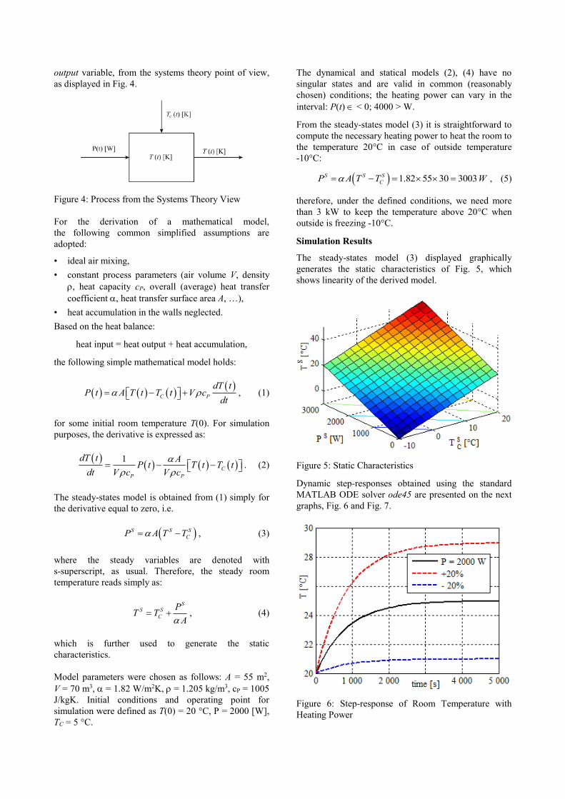
Simulation Results

The steady-states model (3) displayed graphically

generates the static characteristics of Fig. 5, which

shows linearity of the derived model.

Figure 5: Static Characteristics

Dynamic step-responses obtained using the standard

MATLAB ODE solver ode45 are presented on the next

graphs, Fig. 6 and Fig. 7.

Figure 6: Step-response of Room Temperature with

Heating Power

The first one shows the case of different heating power,

starting with the nominal (P = 2000 W) and then small

variations 20% from this value. As can be seen, when

the outside temperature is around 5 °C, the electric

heater enables to heat up the room to 25 °C

approximately, when the power decreases to 1600 W,

the room temperature will be around 21 °C and with

20% more (2400 W) the temperature settles around 29

°C, for the same initial conditions.

Figure 7: Step-response of Room Temperature with

Outside Temperature

The second graph shows the case of different outside

temperature and constant (nominal) power. As expected,

lower outdoor temperature results in lower indoor

temperature and vice versa.

Presented behaviour of the simplified mathematical

model corresponds to the general expectation, therefore

the model can be further used for e.g. subsequent control

system design and analysis. More computations using

the MATLAB software generated 3D plots of Fig. 8-9

with continuous intervals of heating power and outside

temperature.

Figure 8: Step-responses of Room Temperature with

Heating Power – 3D

Figure 9: Step-responses of Room Temperature with

Outside Temperature – 3D

Classification of the Model

Based on the adopted mathematical model and presented

simulation results it is possible to classify it as:

• linear 1st order stable aperiodic system,

• with lumped parameters,

• continuous-time,

• deterministic,

• two-input and single-output,

• time-invariant,

which can further help to design a convenient control

system for the adopted mathematical model, and real

process as well.

Presented information and results outlined a possible

form of students’ final projects in the mentioned course

focused on process modelling and simulation.

CONCLUSIONS

This paper has presented the structure and contents of

the course “Analysis and Simulation of Technological

Processes” taught in the first year of Master’s degree

study programme “Automatic Control & Informatics” at

Faculty of Applied Informatics, Tomas Bata University

in Zlin, Czech Republic. Requirements for the students

to complete the course were also given together with

some statistics concerning their successfulness. The

presented case study has shown one of the simpler final

students’ projects for which the MATLAB computing

system and its toolboxes for simulation and optimization

are fruitfully utilized during the course. Future direction

of the course aims to more practically-oriented

modelling and simulation, connected to practical real-

life examples and actual projects with industrial

companies. There is also an obvious effort to teach the

students not only to build reasonable process models but

also to be able to utilize them for the next step - control

system design. Therefore, in the next semester, after

successful completion of the course “Analysis and

Simulation of Technological Processes” students use

their built models in the next course – “State-space and

Algebraic Control Theory” where they are taught how to

design a convenient control systems. This course is also

completed by a “final project” where students try to

design and implement suitable control algorithms for

their models/systems, again, with the strong help of

MATLAB and Simulink.

REFERENCES

Andaloro, G.; V. Donzelli and R.M. Sperandeo-Mineo. 2007.

“Modelling in physics teaching: the role of computer

simulation.” International Journal of Science Education,

Vol.13, No.3, 243-254.

Bequette, B.W. 2003. Process Control: Modeling, Design and

Simulation. Prentice Hall, New Jersey.

Egeland O. and J.T. Gravdahl. 2002. Modeling and

Simulation for Automatic Control. Marine Cybernetics,

Trondheim.

European Union. 2015. ECTS User's Guide. Publications

Office of the European Union. Luxembourg.

Faculty of Applied Informatics, Tomas Bata University in

Zlin. 2017. [online]. Available at: http://www.utb.cz/fai-en

Jenvald J. and M. Morin. 2004. “Simulation-Supported Live

Training for Emergency Response in Hazardous

Environments.” Simulation and Gaming, Vol.35, No.3,

363-377.

Kincaid, J.P.; R. Hamilton, R.W. Tarr and H. Sangani. 2003.

“Simulation in Education and Training”. In Applied

System Simulation: Methodologies and Applications, M.S.

Obaidat and G.I. Papadimitriou (Eds.). Springer Science,

New York, 437-456.

Lean, J.; J. Moizer; M. Towler and C. Abbey. 2006.

“Simulation and games: Use and barriers in higher

education.” Active learning in higher education, Vol.7,

No.3, 227-242.

Ljung L. and G. Torkel. 1994. Modeling of Dynamic Systems.

Prentice Hall, New Jersey.

Severance, F.L. 2001. System Modeling and Simulation:

An Introduction. Wiley, Chichester.

Skarka W; M. Otrebska and P. Zamorski. 2013. “Simulation

of Dangerous Operation Incidents in Designing Advanced

Driver Assistance Systems” Proceedings of the Institute of

Vehicles, Vol.96, No.5, 131-139.

Stoffa, V. 2004. “Modelling and Simulation as a Recognizing

Method in Education” Educational Media International,

Vol.41, No.1, 51-58.

Thomas, P. 1999. Simulation of Industrial Processes for

Control Engineers. Butterworth-Heinemann, Oxford.

Zavalani, O. and J. Kacani. 2012. “Mathematical Modelling

and Simulation in Engineering Education”. In

Proceedings of the 15th International Conference on

Interactive Collaborative Learning (ICL) (Villach,

Austria, Sep. 26-28). IEEE, Picataway, N.J., 1-5.

AUTHOR BIOGRAPHIES

FRANTIŠEK GAZDOŠ was born in

Zlín, Czech Republic in 1976, and

graduated from the Brno University of

Technology in 1999 with MSc. degree in

Automation. He then followed studies of

Technical Cybernetics at Tomas Bata

University in Zlín, obtaining Ph.D. degree in 2004. He

became Associate Professor for Machine and Process

Control in 2012 and now works as the Head of the

Department of Process Control, Faculty of Applied

Informatics of Tomas Bata University in Zlín.

He is author or co-author of more than 80 journal

contributions and conference papers giving lectures at

foreign universities, such as University of Strathclyde

Glasgow, Instituto Politécnico do Porto, Università di

Cagliari and others. His research covers the area of

process modelling, simulation and control. His e-mail

address is: gazdos@fai.utb.cz.