öMmföäflsäafaäsflassflassflas

fffffffffffffffffffffffffffffffffff

Discussion Papers

Teaching business cycles with the IS-TR model

Juha Tervala University of Helsinki and HECER

Discussion Paper No. 382 August 2014

ISSN 1795-0562

HECER – Helsinki Center of Economic Research, P.O. Box 17 (Arkadiankatu 7), FI-00014 University of Helsinki, FINLAND, Tel +358-9-191-28780, Fax +358-9-191-28781, E-mail info-hecer@helsinki.fi, Internet www.hecer.fi

HECER Discussion Paper No. 382

Teaching business cycles with the IS-TR model Abstract Business cycles are an essential part of macroeconomics. However, the study of macroeconomics often ignores the observed business cycles. During and after the global financial crisis, several economists have emphasized that macroeconomics courses will have to be changed. This paper presents a real world application of the IS-TR model, which helps to explain and teach business cycles. The simple Keynesian model clearly explains output fluctuations and the conduct of monetary policy. The main reason for strong business cycles in the euro area has been shocks in the goods market. The European Central Bank has changed its main interest rate mainly as a reaction to changes in the output gap. JEL Classification: A20, E40, E52 Keywords: business cycles, IS-TR model, macroeconomics, teaching of economics Juha Tervala Department of Political and Economic Studies University of Helsinki P.O. Box 17 (Arkadiankatu 7) FI-00014 University of Helsinki FINLAND e-mail: juha.tervala@helsinki.fi

1. Introduction

Business cycles are an essential part of macroeconomics. The IS-LM model and its successor, the IS-

TR model, are classical tools of macroeconomics teaching. However, the study of macroeconomics

often ignores the observed business cycles. During and after the global financial crisis, several

economists have emphasized that macroeconomics courses will have to be changed. Blinder (2010,

385), for instance, argues that the global financial crisis “should force everyone who teaches

macroeconomics […] to reconsider their curriculums.” Shiller (2010) argues that students have felt

that the lectures on macroeconomics bear little relation to the economic crisis. Also students have

expressed a desire to change the way economics is taught. The International Student Initiative for

Pluralism in Economics (2014), for example, argues that “[t]he real world should be brought back

into the classroom.” Friedman (2010) argues that a key lesson of the financial crisis that that “we

live in a monetary economy and therefore aggregate demand and policies that affect aggregate

demand are determinants of real economic outcomes”.

There is demand for an applied model that helps explain the recently observed business cycles. This

paper introduces an application of the textbook IS-TR model of Burda and Wyplosz (2013), which

helps to explain and teach business cycles and the conduct of monetary policy. The paper’s focus is

on the euro area, but the Keynesian model also effectively explains monetary policy and fluctuations

in output in the United States and Great Britain. The paper’s primary target is macroeconomics

teachers interested in teaching business cycles using a recent and interesting example.1

1 This paper complements Chapter 10 of Macroeconomics: A European Text by Burda and Wyplosz (2013).Figures and Excel files used in this presentation can be found at http://blogs.helsinki.fi/jtervala/teaching-business-cycles-with-the-is-tr-model/. The Excel files can be very useful in analysing the case for the UnitedStates, for example, in various exercises. This paper is based on Tervala (2014).

2. A version of the IS-TR model

This section introduces one version of the IS-TR model. The IS curve represents the combinations of

the nominal interest rate (i) and output (Y), which are consistent with equilibrium of the goods

market. Business cycle models typically (including the model of Burda and Wyplosz (2013)) assume

that prices are sticky, and therefore inflation is zero. However, I assume that inflation matches the

inflation target of the European Central Bank (ECB). Therefore, the real interest rate is the nominal

interest rate minus the inflation target, and fluctuations in the nominal interest rate directly change

the real interest rate.

Aggregate demand depends on private consumption (C), investment (I), public demand (G) and net

exports (PCA, for the primary current account). Therefore, the IS curve can be written as follows:

= + + + .

The Taylor rule (TR) has replaced the LM curve in modern business cycle models. The Taylor rule

describes how the central bank should set the interest rate, depending on the target interest rate,

inflation and output gap. The output gap is the deviation of output from its natural or potential level.

As mentioned earlier, inflation is assumed to match the inflation target of the ECB. Therefore, the

Taylor rule can be written as

= ̅+ ,

where ̅is the target interest rate of the central bank, and b is a parameter governing the central

bank’s response to the output gap, denoted by . The Taylor rule represents the combinations of

output and interest rate that characterize the central bank’s monetary policy. The TR curve moves

only if monetary policy is changed. The central bank responds to fluctuations in the output gap. For

example, a negative output gap implies that the central bank lowers the interest rate below the

target rate. Changes in the target rate move the TR curve. For example, an expansionary

(contractionary) monetary policy shock moves the TR curve downward (upward).

Equilibrium in the short term is the combination of the interest rate and output that satisfies the IS

equation and the Taylor rule. The IS-TR model can be used to analyse the macroeconomic effects of

shocks. Good market shocks shift the IS curve, whereas monetary policy shocks shift the TR curve.

Traditional business cycle models analyse changes in the level of output. However, economic growth

is a pervasive phenomenon. Therefore, I analyse a version of the IS-TR model that focuses on the

output gap, not the level of output. In this version of the model, the IS curve remains at the original

position, assuming aggregate demand growths at the same rate as the potential output. If aggregate

demand growths faster (slower) than potential output, then IS curve shifts rightward (leftward).

Figure 1 shows the IS-TR model in a case where the output gap is zero and the interest rate matches

the target rate of the central bank.

Figure 1. IS-TR model

3. Business cycles in the euro area

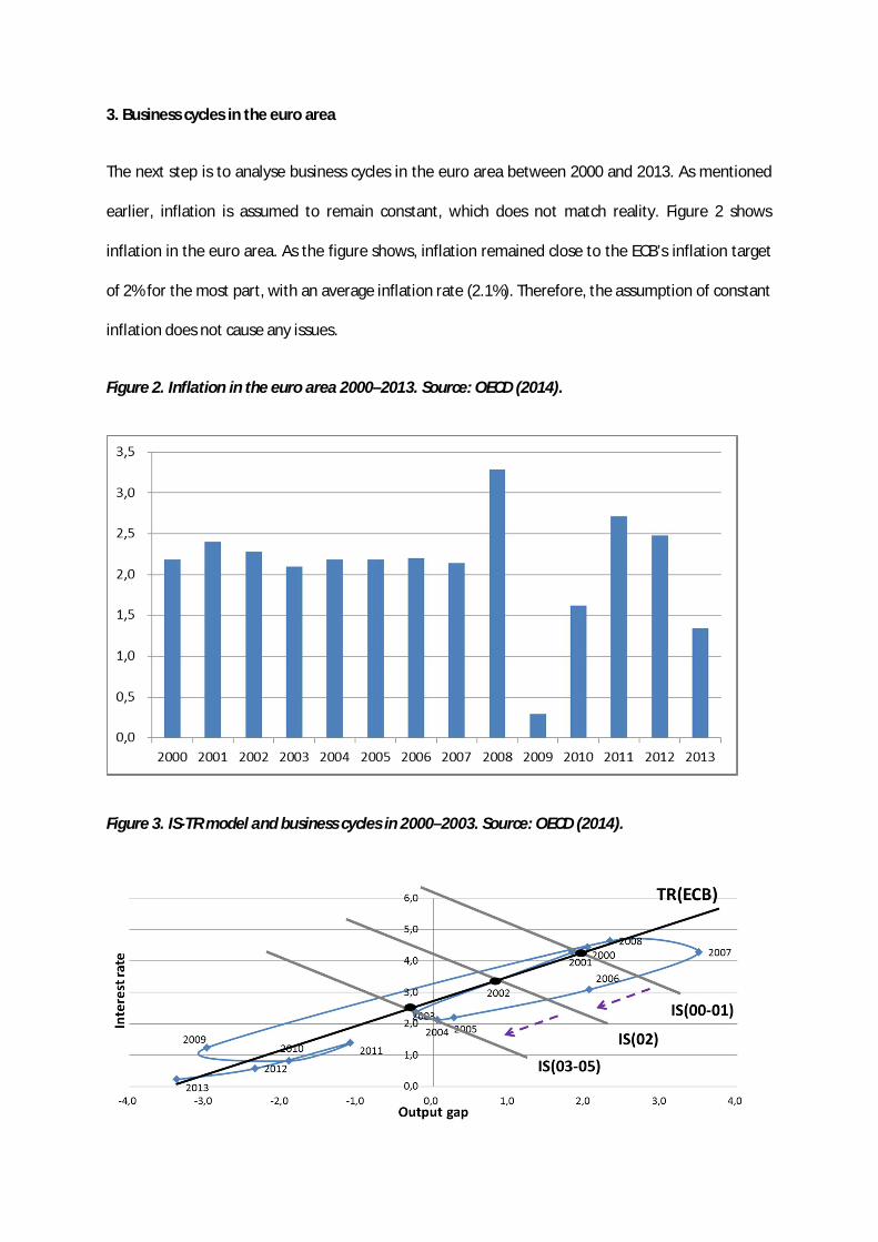
The next step is to analyse business cycles in the euro area between 2000 and 2013. As mentioned

earlier, inflation is assumed to remain constant, which does not match reality. Figure 2 shows

inflation in the euro area. As the figure shows, inflation remained close to the ECB’s inflation target

of 2% for the most part, with an average inflation rate (2.1%). Therefore, the assumption of constant

inflation does not cause any issues.

Figure 2. Inflation in the euro area 2000–2013. Source: OECD (2014).

Figure 3. IS-TR model and business cycles in 2000–2003. Source: OECD (2014).

In Figure 3, the horizontal axis shows the OECD’s estimates of the output gap and the vertical axis

shows the short-term interest rate (three-month money market rate). The money market rate is

used instead of the ECB’s main refinancing rate. This is because the ECB’s main interest rate and

expectations about it are reflected in the three-month money market rate. The short-term interest

rate of several countries is also easily available on the OECD’s website. The data of the United States

and Great Britain, for example, can be used in various exercises. In Figure 3, the TR(ECB) curve

reflects the ECB’s monetary policy rule in the periods of 2000–2003 and 2008–2013. Figure 3 shows

that the ECB’s target rate was 2.7%, and it reacted consistently to changes in the output gap. So

Therefore, the slope of the TR(ECB) curve is realistic (0.8).

Figure 4. Economic growth in the euro area. Source: OECD (2014).

The slope of the IS curves in the figure is -1. Increase in output in the model is due to monetary

policy shocks, when movement takes place along the IS curve. Therefore, the slope of the IS curve is

set to match the effectiveness of monetary policy. A typical estimate calculates the effect of one

percentage change in the interest rate on output to somewhat less than 1%. For example, Christano

et al. (1999) estimate that a positive shock to the monetary policy rule of 75 basis point decreases

output roughly by 0.3% to 0.4%. On the other hand, Bluedorn and Bowdler (2011) estimate that a

one percentage point change in the interest rate changes output by 1.3% to 2.1%. These studies

show that one percentage point shock to the interest rate changes output both by less than 1% and

by more than 1%. Therefore, the assumption that one percentage point change in the interest rate

changes the output gap by 1% can be considered a realistic estimate.

The starting point in Figure 3 is the year 2000. The IS(00) depicts the IS curve in 2000. As mentioned

earlier, TR(ECB) shows the ECB’s normal monetary policy rule. The intersection of the IS(00) and

TR(ECB) curve shows the combination of the interest rate and the output gap in which the money

and goods markets are in equilibrium. Strong economic growth in the late 1990s and in 2000 meant

that in 2000, the interest rate was 4.4% and the output gap 2%. In 2001, economic growth was 2%

and the increase in aggregate demand was roughly equal to that of potential output. Therefore, the

IS curve remained at the same position and the equilibrium was roughly the same as in 2000.

Figure 5. The main interest rate of the ECB. Source: ECB (2014).

In 2002 and 2003, economic growth was slower than usual, as Figure 4 shows. The increase in

aggregate demand was slow, which means that the IS curve shifted leftward. In Figure 3, IS(02)

depicts the IS curve in 2002. The IS curve also shifted leftward in 2003. The IS-TR model implies that

the central bank reacts to this by lowering the interest rate, and the output gap approaches zero.

Figure 5 shows the main interest rate of the ECB. As shown earlier in Figure 3, slow economic growth

and leftward movement of the IS curve in 2002 and 2003 meant that the ECB lowered its main

interest rate several times. This seems to have been a reaction to the change in the output gap

caused by a decrease in demand. Therefore, the fall in the interest rate was a movement along the

TR curve in 2002 and 2003. In 2003, the interest rate was 2.4% and the output gap was negative.

Figure 6. IS-TR model and business cycles in 2003–2007. Source: OECD (2014).

The IS(03-05) curve in Figure 6 shows the IS curve for the period 2003–2005. As shown earlier in

Figure 5, the ECB lowered the interest rate in 2003 to the 2% level, where it was kept for some time.

In 2004, it seems that the ECB caused an expansionary monetary policy shock that shifted the TR

curve downward. The ECB seems to have pursued expansionary monetary policy between 2004 and

2007. In Figure 6, the TR(04-07) shows the ECB’s TR curve for 2004–2007. In 2004, the economy

moved along the IS curve to new equilibrium. The interest rate lowered and the output gap turned

positive. In 2005, economic growth in the euro area was normal (2%) and the IS curve remained

roughly at the same place. Therefore, the money market interest rate was slight above 2% and the

output gap was slightly above zero, just as in 2004.

Economic growth was much faster than normal in 2006–2007, as aggregate demand increased

rapidly for several reasons. First, a consumption boom took place in several euro area countries.

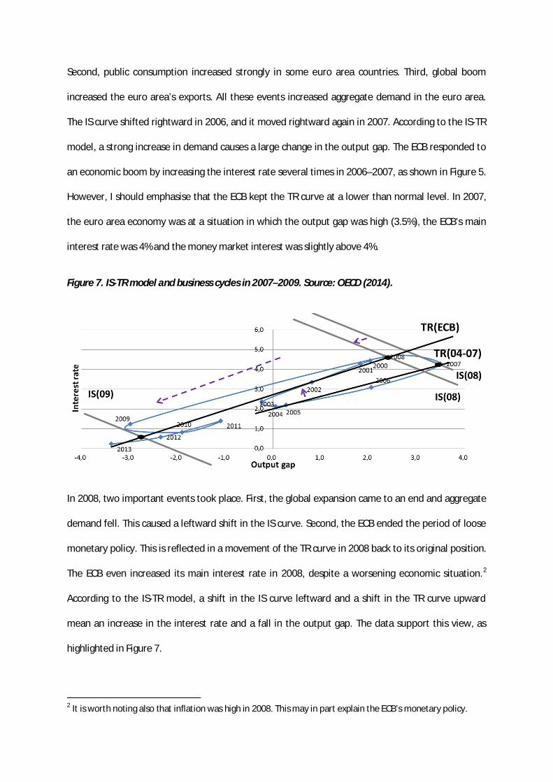
Second, public consumption increased strongly in some euro area countries. Third, global boom

increased the euro area’s exports. All these events increased aggregate demand in the euro area.

The IS curve shifted rightward in 2006, and it moved rightward again in 2007. According to the IS-TR

model, a strong increase in demand causes a large change in the output gap. The ECB responded to

an economic boom by increasing the interest rate several times in 2006–2007, as shown in Figure 5.

However, I should emphasise that the ECB kept the TR curve at a lower than normal level. In 2007,

the euro area economy was at a situation in which the output gap was high (3.5%), the ECB’s main

interest rate was 4% and the money market interest was slightly above 4%.

Figure 7. IS-TR model and business cycles in 2007–2009. Source: OECD (2014).

In 2008, two important events took place. First, the global expansion came to an end and aggregate

demand fell. This caused a leftward shift in the IS curve. Second, the ECB ended the period of loose

monetary policy. This is reflected in a movement of the TR curve in 2008 back to its original position.

The ECB even increased its main interest rate in 2008, despite a worsening economic situation.2

According to the IS-TR model, a shift in the IS curve leftward and a shift in the TR curve upward

mean an increase in the interest rate and a fall in the output gap. The data support this view, as

highlighted in Figure 7.

2 It is worth noting also that inflation was high in 2008. This may in part explain the ECB’s monetary policy.

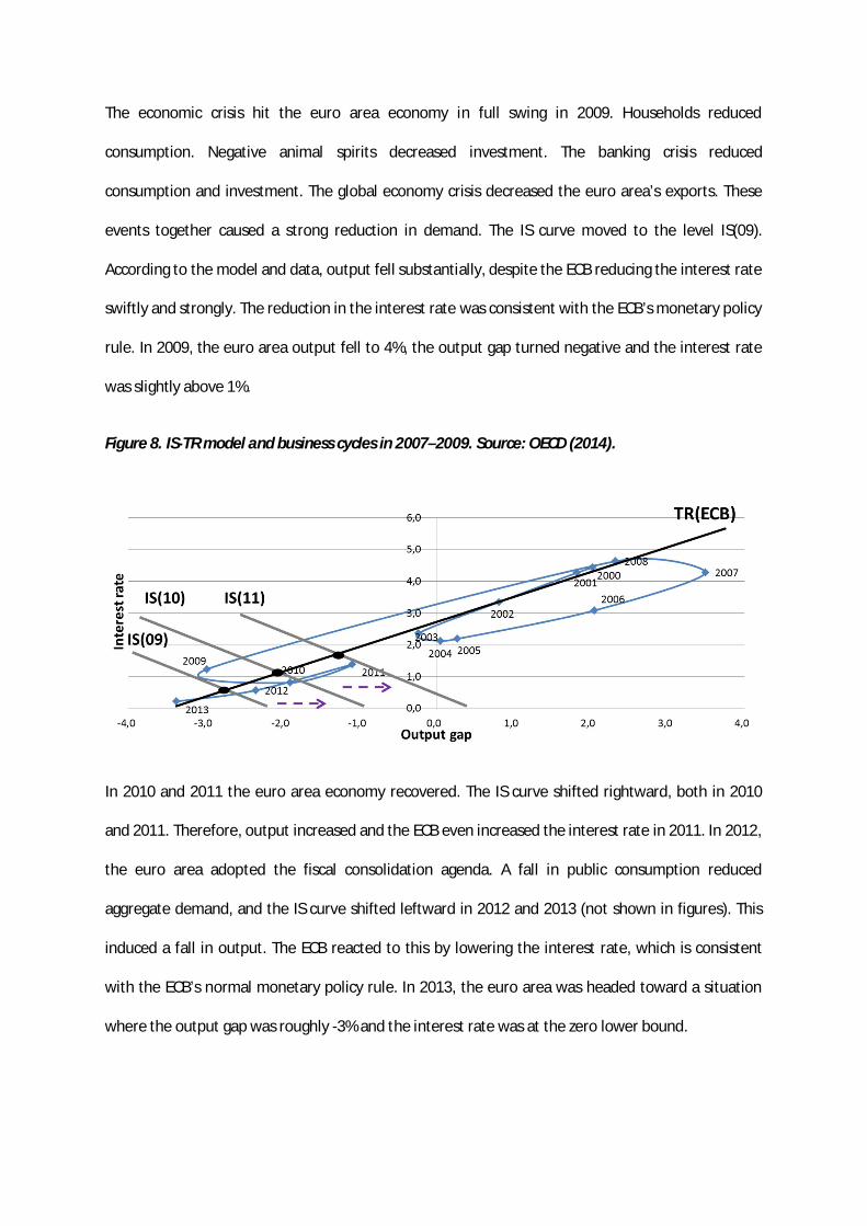
The economic crisis hit the euro area economy in full swing in 2009. Households reduced

consumption. Negative animal spirits decreased investment. The banking crisis reduced

consumption and investment. The global economy crisis decreased the euro area’s exports. These

events together caused a strong reduction in demand. The IS curve moved to the level IS(09).

According to the model and data, output fell substantially, despite the ECB reducing the interest rate

swiftly and strongly. The reduction in the interest rate was consistent with the ECB’s monetary policy

rule. In 2009, the euro area output fell to 4%, the output gap turned negative and the interest rate

was slightly above 1%.

Figure 8. IS-TR model and business cycles in 2007–2009. Source: OECD (2014).

In 2010 and 2011 the euro area economy recovered. The IS curve shifted rightward, both in 2010

and 2011. Therefore, output increased and the ECB even increased the interest rate in 2011. In 2012,

the euro area adopted the fiscal consolidation agenda. A fall in public consumption reduced

aggregate demand, and the IS curve shifted leftward in 2012 and 2013 (not shown in figures). This

induced a fall in output. The ECB reacted to this by lowering the interest rate, which is consistent

with the ECB’s normal monetary policy rule. In 2013, the euro area was headed toward a situation

where the output gap was roughly -3% and the interest rate was at the zero lower bound.

4. Conclusions

This paper is an attempt to bring the real world into macroeconomics lectures. The paper introduces

a version of the IS-TR model, which helps teach the observed business cycles in an interesting way.

The simple Keynesian model clearly explains output fluctuations and the conduct of monetary policy.

Analysis indicated that shocks in the goods markets have been the driving force of business cycles in

the euro area. The ECB has increased and decreased its main interest rate mainly as a response to

changes in the output gap. Most of the time, the ECB’s monetary policy has been consistent with the

Taylor rule. However, the ECB implemented expansionary monetary policy in 2004–2007. This was a

contributing factor to the overheating of the economy in 2006–2007. However, analysis indicates

that the overheating, and the long economic crisis of 2009–2013, were mainly caused by shocks in

the goods markets.

References

Blinder, A. 2010. Teaching Macro Principles after the Financial Crisis, Journal of Economic Education

40 (4): 385–390.

Bluedorn, J.C. and Bowdler, C. 2011. The open economy consequences of U.S. monetary policy,

Journal of International Money and Finance 30 (2): 309–36.

Burda, M. and Wyplosz, C. 2013. Macroeconomics: A European Text, 6th edition, Oxford, Oxford

University Press.

Christiano, L., Eichenbaum, M. and Evans, C. 1999. Monetary policy shocks: What have we learned

and to what end? in Handbook of Macroeconomics 1A, ed. Taylor, J. and Woodford, M,

Amsterdam, Elsevier Science.

ECB 2014. Statistics. https://www.ecb.europa.eu/stats/html/index.en.html (accessed May 12, 2014).

Friedman, B. M. 2010. Reconstructing Economics in Light of the 2007–? Financial Crisis. Journal of

Economic Education 40 (4), 391–397.

International Student Initiative for Pluralism in Economics 2014. An international student call for

pluralism in economics. http://www.isipe.net/open-letter/ (accessed May 15, 2014).

OECD 2014. Economic Outlook Annex Tables,

http://www.oecd.org/economy/outlook/economicoutlookannextables.htm (accessed May 13,

2014).

Shiller, R. 2010. How Should the Financial Crisis Change How We Teach Economics?. Journal of

Economic Education 40 (4), 403–409.

Tervala, J. 2014. Euroalueen suhdannevaihteluiden opettaminen. Kansantaloudellinen aikakauskirja

(Finnish Economic Journal) 110 (2), 202–210.