TB Or Not TB?

by

Samuel R. Baty, Peter J. Armijo, Claire E. Armijo,

and Sarah M. Baty

Team 52

Los Alamos High School, Los Alamos, NM 87544

Teacher: Mr. Lee Goodwin of Los Alamos High School.

Mentors: Dr. Don H. Tucker, Professor of Mathematics of the University of Utah,

Mrs. Joanne V. Baty of Los Alamos,

Dr. Roy S. Baty of Los Alamos National Laboratory.

Abstract

This report studies the epidemiology of Tuberculosis (TB) with

emphasis on the evolution of TB within a population exposed to TB

in the Middle East. American troops fighting overseas have been ex-

posed to this disease and could potentially spread it to the general

population. A dynamical system was used to model the evolution of

TB. The epidemiology of TB was modeled with existing disease pa-

rameters for an idealized problem representing the population in the

region surrounding Santa Fe, New Mexico. The epidemiology simula-

tions imply that increased troop exposure could lead to a few thousand

more cases of TB in New Mexico over the next 150 years.

1

1 Introduction

This report explores the epidemiology of Tuberculosis (TB). The spread of

Tuberculosis has always been an issue in America, and is especially a prob-

lem now because of American troops fighting overseas in the Middle East

acquiring it, and then returning home with this disease and possibly spread-

ing it throughout the general population. Many of these soldiers have an

antibiotic-resistant strain of TB, making this problem even more alarming in

our society today.

In this project, a dynamical system with five ordinary differential equa-

tions was used to model the evolution of TB in time. A program was devel-

oped to integrate the equations modeling the evolution of the disease. We

modeled the spread of the disease with existing disease parameters for an ide-

alized problem representing the population in the region surrounding Santa

Fe, New Mexico. We then doubled the proportion of new infections of the

disease to estimate the long term effects of the TB epidemiology associated

with the increased exposure to our troops. The results for the model of the

existing disease were compared to that with the increased exposure and the

differences in the time history of TB was analyzed.

A seventh-order Runge-Kutta-Fehlberg scheme was implemented to nu-

merically integrate the epidemiology model. This numerical method was

applied to study the stability for both linear and nonlinear cases. Mathe-

matica was also applied to construct analytical solutions to check the numer-

ical results for a simplified case. The solutions were found to be stable and

approach equilibrium states. The numerical scheme was coded using the lan-

guage C. All plots for this project were generated using the software program

Gnuplot. All analytical estimates were performed using Mathematica. The

computer that performed all calculations is a Mac with a 10.6.8 operating

system. The C and Mathematica programs developed for the project are

listed in the Appendices.

2

2 Background Information and the

Epidemiology of Tuberculosis

Tuberculosis is an urgent health issue today, because a new antibiotic-resistant

strain has emerged in the Middle East among other places, and is currently

coming home with American troops. There has been an ongoing effort in

developing a new TB vaccine, with no successful results yet. Our own Uni-

versity of New Mexico was awarded a grant from the Bill and Melinda Gates

Foundation for developing this vaccine by pharmacy professor Dr. Pavan

Muttil, Jetty [1], because of the threat seen here in the United States and

worldwide from a new, untreated TB strain. The study is still ongoing.

There was another, larger study out of the University of Oxford for a vaccine

called MVA85A that replaced the Bacille Calmette-Guerin (or BCG) that

was developed ninety years ago and only works for a few years. This new

MVA85A vaccine, however, failed substantially and hopes are now pinned on

other pending vaccines.

Mycobacterium TB has plagued human kind since antiquity, Blower and

Chou [2]. Blower’s definition of multi-drug-resistant TB (MDRTB) is de-

fined as TB that is resistant to two of the best anti-tuberculosis drugs, which

are Isoniazid and Rifampicin. Right now, MDRTB is only showing up in

localized areas, but the threat of the fast spreading disease is urgent. The

modern global TB epidemic affects nine million people annually and kills

1.4 million each year, Steenhuysen [3]. Tuberculosis, which was known in

history as consumption or the white plague, has been found as far back as

the ancient Egyptian mummies of 3000 B.C. and is thought to have been in

modern human remains in the Neolithic Era dating from 9000 years ago in

the Mediterranean. It was only recently in 1944 that scientists came up with

the first antibiotic of streptomycin that was effective against these mycobac-

terium and it was generally thought to be on its’ way to eradication once

the last patients were treated and cured especially in the 1980s. However,

3

with the rise of drug resistant strains from previous levels of 5000 cases in

1987, has now gone up to 7600 cases in 2005 in Great Britain, for example.

New York currently has more than 20,000 TB patients that have multi-drug

resistant strains, and have to be quarantined in hospitals.

Latest figures show that 45.7 percent of US troops that work in the public

of Afghanistan are showing up with TB exposure, Mitchell et al. [4]. How-

ever, since TB scratch tests are notoriously false-positive, the real figure is

probably somewhat lower. According to Mitchell et al., in the United States,

the percentage of MDRTB cases has increased slowly, from 0.9 percent of

the total number of reported TB cases in 2008 to 1.3 percent of cases in

2011. In the rest of the world, however, particularly in the Middle Eastern

countries Iraq and Afghanistan, this figure in American troops coming down

with MDRTB is 2.9 percent to 10 percent in certain crowded public areas

of Afghanistan. In addition, there is a long-term threat of active TB cases

developing later since latent TB can change into active or contagious TB

if a patient’s immune system fails, as with AIDS patients. Coupled with

rising rates of MDRTB, the computer model in this project below shows a

real threat not only to the US but worldwide. According to this model, this

could turn into a real epidemic. American troops today in active duty are

now being routinely checked for TB infection before and after they go on

their tours of duty, Aronson et al. [5].

3 Mathematical Modeling

3.1 The Dynamical System

The dynamical system modeling the evolution of TB is based on the work of

Blower et al. [6]. The Blower description may be expressed as a system of five

ordinary differential equations. The equations and their stability properties

have been analyzed by Tucker [7]. The basic mathematical model is given

4

by the following five equations:

dX

dt= Π− λX − µX, (1)

dL

dt= (1− p)λX − (ν + µ)L, (2)

dTidt

= pfλX + qνL+ ωR− (µ+ µT + c)Ti, (3)

dTndt

= p(1− f)λX + (1− q)νL+ ωR− (µ+ µT + c)Tn, (4)

anddR

dt= c(Ti + Tn)− (2ω + µ)R. (5)

In Equations (1) to (5), the independent variables are: the susceptible

cases X, the latently infected cases L, the infectious cases Ti, the non-

infectious cases Tn, and the recovered cases R. The parameters in Equa-

tions (1) to (5) are defined in Blower et al. [6], as follows: the average life

expectancy 1/µ, the recruitment rate Π, the proportion of new infections

that develop TB within a year p, the progression rate to TB v, the proba-

bility of developing infectious TB (fast TB) f , the probability of developing

infectious TB (slow TB) q, the mortality rate due to TB µT , the rate of

relapse to active TB 2ω, and the natural cure rate c. The last parameter is

λ the per-susceptible risk of becoming infected. This term is modeled both

as a constant λ = 1 and as a feed-back term λ = βTi in this study. More-

over, a transmission coefficient β is defined so that βΠ/µ = constant. The

application of a constant λ linearizes the dynamical system and allows the

construction of exact analytical solutions in specific cases.

5

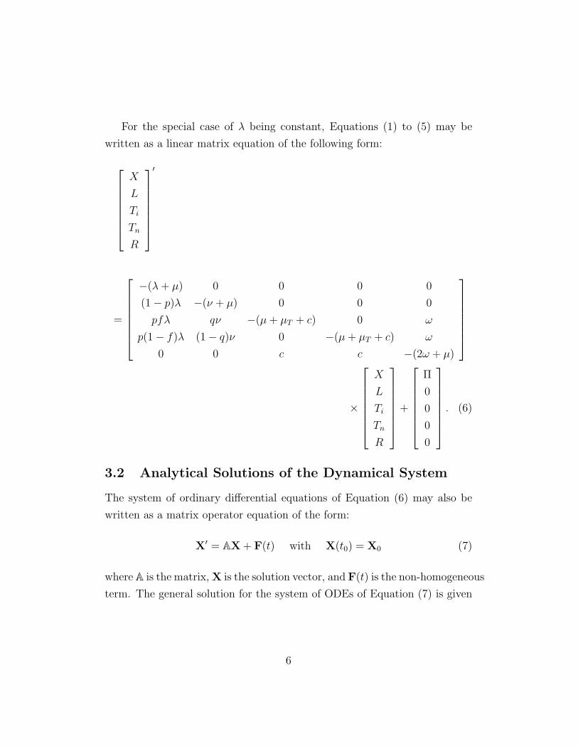
For the special case of λ being constant, Equations (1) to (5) may be

written as a linear matrix equation of the following form:

X

L

Ti

Tn

R

′

=

−(λ+ µ) 0 0 0 0

(1− p)λ −(ν + µ) 0 0 0

pfλ qν −(µ+ µT + c) 0 ω

p(1− f)λ (1− q)ν 0 −(µ+ µT + c) ω

0 0 c c −(2ω + µ)

×

X

L

Ti

Tn

R

+

Π

0

0

0

0

. (6)

3.2 Analytical Solutions of the Dynamical System

The system of ordinary differential equations of Equation (6) may also be

written as a matrix operator equation of the form:

X′ = AX + F(t) with X(t0) = X0 (7)

where A is the matrix, X is the solution vector, and F(t) is the non-homogeneous

term. The general solution for the system of ODEs of Equation (7) is given

6

by the matrix equation:

X(t) = exp[A(t− t0)]X0 + exp[A(t)]

∫ t

t0

exp[−A(s)]F(s) ds. (8)

The solution given by Equation (8) for the system of ODES of Equation

(7) is computed by determining the eigenvalues {Ei} and eigenvectors {xi} of

the matrix A (i = 1, 2, 3, 4, 5). Recall that the eigenvalues and eigenvectors

satisfy the relationship Ax = Ex. If the matrix A has 5 distinct real-valued

eigenvalues, then the matrix exponential, exp[A(t)], is computed using the

matrix formula:

exp[A(t)] =[

exp[E1t]x1 exp[E2t]x2 exp[E3t]x3 exp[E4t]x4 exp[E5t]x5

]×

[x1 x2 x3 x4 x5

]−1

. (9)

where {xi} are column vectors. For a derivation of Equation (9), see Braun

[8]. If the matrix A has repeated or complex-valued eigenvalues, the repre-

sentation of the matrix exponential of Equation (9) is more complex and is

beyond the scope of the present study.

3.3 Numerical Method

In this study a seventh-order Runge-Kutta-Fehlberg (RKF) scheme was im-

plemented to integrate the threshold of collapse problems. This scheme em-

ployed variable stepsize control. High-order Runge-Kutta schemes were de-

veloped in astrodynamics, for example see the textbook of Battin [9].

The scheme applied in this study was developed by Fehlberg [10], and is

defined by the following equations:

f0 = f(x0, y0), (10)

7

fκ = f(x0 + ακh, y0 + hκ−1∑λ=0

βκλfλ), (11)

y = y0 + h

10∑κ=0

cκfκ + 0(h8), (12)

and

y = y0 + h12∑κ=0

cκfκ + 0(h9), (13)

where h is the step size. In Equation (11), κ = 1, 2, 3, ..., 12. An ordinary

differential equation is integrated numerically by applying Equations (10),

(11), and (12) in an iterative fashion. Equation (10) represents the system of

equations to be integrated at the initial data point, (x0, y0). Equations (12)

and (13) are the seventh and eighth-order RKF schemes, respectively. Equa-

tion (12) is used to calculate the solution. Equation (13) is used to compute

the stepsize update. In Equations (11), (12), and (13), there are quadrature

constants, ακ, βκλ, cκ, cκ, required by the numerical method, Fehlberg [10]

(see page 65).

The seventh-order Runge-Kutta-Fehlberg scheme is used in this study be-

cause the solutions may have highly nonlinear characteristics. For example,

nonlinear problems may have solutions that become very sensitive to the ini-

tial conditions. The RKF numerical method allows the accurate calculation

of data when the rate of change of the solution is very small and very large.

In addition to the analytical solutions constructed with Mathematica, the

RKF code developed for this project was checked against known solutions to

a linear vibration problem. For an outline of the validation problem and its

solution, see Baty and Armijo [11].

8

3.4 The Stability of Dynamical Systems

The qualitative theory of ordinary differential equations is the study of the

global behavior of solutions to ODEs including their stability. Stability, in the

context of this project, was defined as the long-time behavior of a solution of a

dynamical system, Sanchez [12]. A stable system in an epidemiology model

approaches an equilibrium set. The characteristics of a non-stable system

would include the rate of change of the solution growing without bound, or

the system suddenly exploding around a fixed value. In this study numerical

experiments were used to determine whether or not the model problems are

stable.

The analysis of all of the numerical experiments was done by plotting

components of the solutions of the system in phase space. Phase space is

defined as a five-dimensional representation of the solutions to the given

ODEs, Arnold [13]. The goal of the analysis was to discover the solutions

that reach equilibrium points. A given system of ODEs represents a slope

field in the region of phase space where the equations are defined. A solution

of the system is a curve in phase space that is tangent to the slope field

defined by the differential equations for each point on the curve.

4 Epidemiology of Tuberculosis

4.1 Analytical Example

To begin studying the TB model given by Equation (6), an analytical solution

to this system is built for a simple case. The parameters in the model are

defined as follows:

Π = 25.00, λ = 1.00, µ = 0.02, p = 0.175, c = 0.058, µT = 0.139, (14)

9

and

ω = 0.005, f = 0.70, q = 0.50, ν = 0.003915. (15)

The values from Equations (14) and (15) are substituted into Equations (1)

to (5) and the eigenvalues are eigenvectors are computed using Mathematica.

The eigenvalues for this problem are real-valued and distinct. The calcula-

tion of the eigenvalues and eigenvectors the resulting matrix, A, is shown in

Appendix B.

Using the eigenvalues and eigenvectors, the exponential of the matrix

exp[A(t)] may be computed using:

exp[A(t)] = exp[−1.02t]M1 + exp[−0.220052t]M2

+ exp[−0.217t]M3 + exp[−0.0269482t]M4 + exp[−0.023915t]M5, (16)

where

M1 =

1.0 0 0 0 0

−0.828243 0 0 0 0

−0.150612 0 0 0 0

−0.0634389 0 0 0 0

0.0125404 0 0 0 0

, (17)

M2 =

0 0 0 0 0

0 0 0 0 0

0.0975233 −0.00982255 0.492098 0.492098 −0.0258928

0.0975233 −0.00982255 0.492098 0.492098 −0.0258928

−0.0595243 0.00599529 −0.300357 −0.300357 0.0158039

,(18)

M3 =

0 0 0 0 0

0 0 0 0 0

0.0435866 0 0.5 −0.5 0

−0.0435866 0 −0.5 0.5 0

−7.25862 0 −83.2667 83.2667 0

, (19)

10

M4 =

0 0 0 0 0

0 0 0 0 0

−0.0070807 −0.0101992 0.00790197 0.00790197 0.0258928

−0.0070807 −0.0101992 0.00790197 0.00790197 0.0258928

−0.26914 −0.387675 0.300357 0.300357 0.984196

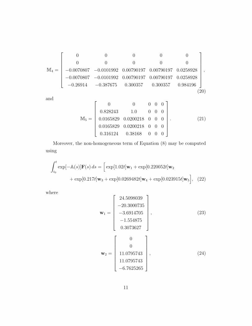
,(20)

and

M5 =

0 0 0 0 0

0.828243 1.0 0 0 0

0.0165829 0.0200218 0 0 0

0.0165829 0.0200218 0 0 0

0.316124 0.38168 0 0 0

. (21)

Moreover, the non-homogeneous term of Equation (8) may be computed

using

∫ t

t0

exp[−A(s)]F(s) ds =[

exp[1.02t]w1 + exp[0.220052t]w2

+ exp[0.217t]w3 + exp[0.0269482t]w4 + exp[0.023915t]w5

], (22)

where

w1 =

24.5098039

−20.3000735

−3.6914705

−1.554875

0.3073627

, (23)

w2 =

0

0

11.0795743

11.0795743

−6.7625265

, (24)

11

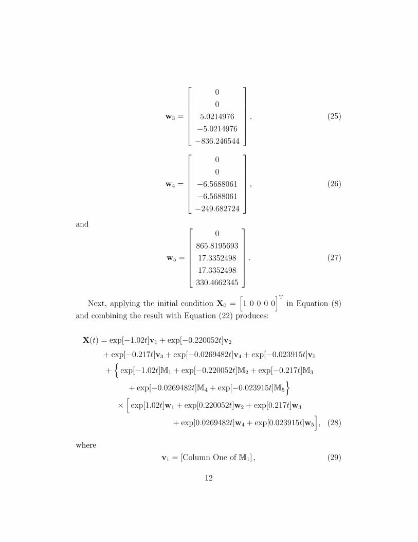
w3 =

0

0

5.0214976

−5.0214976

−836.246544

, (25)

w4 =

0

0

−6.5688061

−6.5688061

−249.682724

, (26)

and

w5 =

0

865.8195693

17.3352498

17.3352498

330.4662345

. (27)

Next, applying the initial condition X0 =[1 0 0 0 0

]T

in Equation (8)

and combining the result with Equation (22) produces:

X(t) = exp[−1.02t]v1 + exp[−0.220052t]v2

+ exp[−0.217t]v3 + exp[−0.0269482t]v4 + exp[−0.023915t]v5

+{

exp[−1.02t]M1 + exp[−0.220052t]M2 + exp[−0.217t]M3

+ exp[−0.0269482t]M4 + exp[−0.023915t]M5

}×

[exp[1.02t]w1 + exp[0.220052t]w2 + exp[0.217t]w3

+ exp[0.0269482t]w4 + exp[0.023915t]w5

], (28)

where

v1 = [Column One of M1] , (29)

12

v2 = [Column One of M2] , (30)

v3 = [Column One of M3] , (31)

v4 = [Column One of M4] , (32)

and

v5 = [Column One of M5] . (33)

Equation (28) is the analytical solution of the linear problem defined by

Equations (6) with the parameters of Equations (14) and (15) and the initial

condition X0 =[1 0 0 0 0

]T

.

Equation (28) has been used to check the C code developed to solve the

dynamical system used to model the evolution of TB. For example, Equation

(28) may be used to show that the solution to the first variable approaches

X(t)→ 24.5098039 as t→∞, which is in agreement with the computational

result.

4.2 Numerical Example: A Linear Model for

Northern New Mexico

In this section a simple model is described and applied to study the effects on

the evolution of TB in New Mexico caused by troop exposure in the Middle

East. Parameters from a published model are used to represent a baseline or

unperturbed evolution of TB. The effects of troop exposure are then modeled

by changing the proportional constant p associated with new infections. From

Mitchell et al. [4], the number of new infections is assumed to approximately

double because of the troop exposure. The war (troop exposure) is assumed

to last for 20 years. To estimate the behavior of the disease in a community

13

surrounding Santa Fe, New Mexico, the following initial data is assumed:

X0 =

X

L

Ti

Tn

R

=

120, 000

0

1

0

0

, (34)

where the initial data implies that at the beginning of the disease time history

that there are 120,000 susceptible individuals and one infectious case. It

is assumed that there are approximately 120,000 individuals in the region

surrounding Santa Fe that are susceptible to TB. The model consists of the

initial data of Equation (34) and Equations (1) to (5) with the following

parameters:

Π = 4400, µ = 0.0222, c = 0.058, µT = 0.139, (35)

and

ω = 0.005, f = 0.70, q = 0.85, ν = 0.00256, (36)

Blower, et al [6]. The proportional constant associated with new infections

is assumed to be given by:

p =

0.10 if t < 20

0.05 if t ≥ 20, (37)

which is used to represent the increased exposure to TB of the troops in the

Middle East. The per-susceptible risk of becoming infected is modeled as

λ = 1.0, (38)

14

for the first example. Equation (38) guarantees that the governing dynamical

system, Equation (6), will be linear.

Figures 1 through 5 show the results for the linear epidemiology model

of Tuberculosis. Figure 1 shows the number of susceptible cases of TB for

the constant values of p = 0.1, p = 0.05, and the values of Equation (37). In

figure the number of susceptible cases is the same for each value of p, however

this number occurs at different times in evolution of the disease.

Figures 2 through 4 show the latent, infectious and non-infectious cases,

respectively. Each figure shows the transition of the linear evolution of TB

at 20 years from the p = 0.1 solution to the p = 0.05 solution. Figure 5

shows the number of recovered cases for the two constants.

For this example, the matrix A associated with the dynamical system

of Equation (6) has five, distinct, real-valued eigenvalues. The eigenvalues

are all negative, which implies the solution will be stable in time. Figures

2 through 5 show the asymptotic values to which the independent variables

X,L, Ti, Tn, and R converge. The solution of the dynamical system suggests

that the disease approaches the equilibrium values after about 120 years.

Hence the time-scale associated with a perturbation in TB is on the order of

several decades.

15

Figure 1: Solutions for the simple linear model for X, the susceptible cases.The vertical axis is number of cases and the horizontal axis is time in years.The red and blue curves assume the constant values of p = 0.1 and p = 0.05for all time respectively, while the green curve assumes p = 0.1 if t < 20 yearsand p = 0.05 if t ≥ 20 years.

Figure 2: Solutions for the simple linear model for L, the latent cases. Thevertical axis is number of cases and the horizontal axis is time in years. Thered and blue curves assume the constant values of p = 0.1 and p = 0.05 forall time respectively, while the green curve assumes p = 0.1 if t < 20 yearsand p = 0.05 if t ≥ 20 years.

16

Figure 3: Solutions for the simple linear model for Ti, the infectious cases.The vertical axis is number of cases and the horizontal axis is time in years.The red and blue curves assume the constant values of p = 0.1 and p = 0.05for all time respectively, while the green curve assumes p = 0.1 if t < 20 yearsand p = 0.05 if t ≥ 20 years.

Figure 4: Solutions for the simple linear model for Tn, the non-infectiouscases. The vertical axis is number of cases and the horizontal axis is timein years. The red and blue curves assume the constant values of p = 0.1and p = 0.05 for all time respectively, while the green curve assumes p =0.1 if t < 20 years and p = 0.05 if t ≥ 20 years.

17

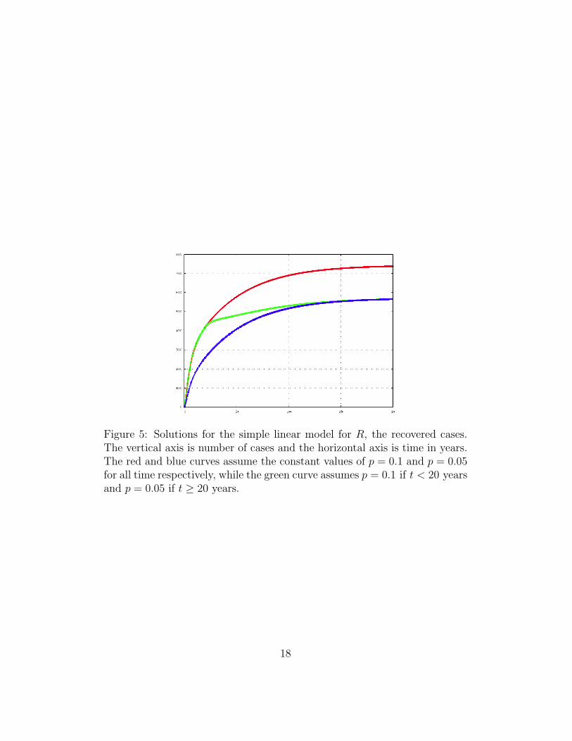
Figure 5: Solutions for the simple linear model for R, the recovered cases.The vertical axis is number of cases and the horizontal axis is time in years.The red and blue curves assume the constant values of p = 0.1 and p = 0.05for all time respectively, while the green curve assumes p = 0.1 if t < 20 yearsand p = 0.05 if t ≥ 20 years.

18

4.3 Numerical Example: A Nonlinear Model for

Northern New Mexico

For the second numerical example, the same problem of Section 4.2 is studied

with the nonlinear feed-back term:

λ = 0.00005 · Ti, (39)

following Blower et al. [6]. In this case the epidemiology model for TB is

defined by Equations (1) through (5), (34) through (37), and (39). Again,

the initial susceptible population is assumed to be 120,000 individuals, and

at time zero one infectious case is present. The effect of the troop exposure

is modeled by Equation (37), which reduces the new infection population

constant by a factor of two after 20 years.

Figures 6 through 10 show the effect of the war (troop exposure) by com-

paring the variable new infection constant, Equation (37), with the constant

new infection value p = 0.05. In Figure 6 the effect of the change in p is

shown. By increasing p the number of susceptible cases decreases during

the war. Figure 7 then shows that the change in p causes the number of

latent cases to increase sooner than the baseline disease model. Figure 7

also shows that TB converges back to the baseline model around 200 years

after the troop exposure is over. This figure implies that the disease changes

a lot about 50 years after the war and then converges back to the baseline

case over the next 100 years. The characteristic time-scale of the disease is

approximately 150 years.

Figures 8 and 9 show the change in infectious and non-infectious cases

caused by the war. The solutions are similar to the latent case in that the

numbers of infectious and non-infectious cases increase sooner than the base-

line disease model. Figures 8 and 9 also show that both of these populations

have localized peaks around 50 years. Figure 10 shows the number of recov-

ered cases associated with the troop exposure.

19

To understand the effect of the troop exposure with respect to the baseline

TB model, Figures 11 through 15 show the differences of the TB war and

the TB baseline models. Figure 11 shows that the war causes an increase of

about 85,000 latent cases of TB at 45 years after the beginning of the war

(25 years after the war is over). This figure also shows a minor decrease in

the number of latent cases 75 years after the beginning of the war. Figures

12 and 13 show the infectious and non-infectious cases caused by the war.

Both of these plots have peaks around 45 years after the beginning of the

war. Figure 12 shows an increase of about 1500 cases of TB 45 years after

the war. Moreover, Figure 13 shows an increase of about 500 cases of TB 45

years after the war. Both Figures 12 and 13 show a decrease in the number

of cases of TB with respect to the baseline model 75 years after the war.

Figure 14 shows the sum of the infectious and non-infectious cases due to the

war. This plot exhibits a peak of 2000 cases approximately 45 years after

the beginning of the war. Figure 15 shows the recovered cases associated

with the war. The recovered cases peak about 60 years after the beginning

of the war and converge back to the baseline model at about 200 years. It

is interesting to note that the recovered cases is strictly positive, because

recovered cases only occur as a result of troop exposure.

The baseline and war TB models show that the evolution of Tuberculosis

lasts on the order of 150 years. Notice that the effect of Equation (37) may

be seen in the infectious and non-infectious cases. For these independent

variables, the solutions show a kink at 20 years, the end of the war. Also

notice, the solutions of the TB epidemiology model are all stable in time and

converge to equilibrium solutions around 200 years.

20

Figure 6: Solutions for the nonlinear model for X, the susceptible cases. Thevertical axis is number of cases and the horizontal axis is time in years. Thered curve is the number of susceptible cases without the war, and the greencurve is the number of susceptible cases with the war.

Figure 7: Solutions for the nonlinear model for L, the latent cases. Thevertical axis is number of cases and the horizontal axis is time in years. Thered curve is the number of latent cases without the war, and the green curveis the number of latent cases with the war.

21

Figure 8: Solutions for the nonlinear model for Ti, the infectious cases. Thevertical axis is number of cases and the horizontal axis is time in years. Thered curve is the number of infectious cases without the war, and the greencurve is the number of infectious cases with the war.

Figure 9: Solutions for the nonlinear model for Tn, the non-infectious cases.The vertical axis is number of cases and the horizontal axis is time in years.The red curve is the number of non-infectious cases without the war, and thegreen curve is the number of non-infectious cases with the war.

22

Figure 10: Solutions for the nonlinear model for R, the recovered cases. Thevertical axis is number of cases and the horizontal axis is time in years. Thered curve is the number of recovered cases without the war, and the greencurve is the number of recovered cases with the war.

Figure 11: Latent cases caused by the war. The vertical axis is number ofcases and the horizontal axis is time in years. Compare with Figure 7.

23

Figure 12: Infectious cases caused by the war. The vertical axis is numberof cases and the horizontal axis is time in years. Compare with Figure 8.

Figure 13: Non-infectious cases cause by the war. The vertical axis is numberof cases and the horizontal axis is time in years. Compare with Figure 9.

24

Figure 14: The sum of infectious and non-infectious cases caused by the war.The vertical axis is number of cases and the horizontal axis is time in years.Compare with Figures 12 and 13.

Figure 15: Recovered cases resulting from the war. The vertical axis isnumber of cases and the horizontal axis is time in years. Compare withFigure 10.

25

5 Summary and Conclusions

This project studied the epidemiology of Tuberculosis (TB) with emphasis

on the evolution of TB within a population exposed to TB in the Middle

East. American troops fighting overseas have been exposed to this disease

and could potentially spread it to the general population.

In our project, a dynamical system was used to model the evolution of TB

in time. A C program was developed to integrate the equations modeling the

evolution of the disease. The epidemiology of TB was modeled with existing

disease parameters for an idealized problem representing the population in

the region surrounding Santa Fe, New Mexico. The proportion of new in-

fections of the disease was doubled on a 20 year time interval to estimate

the long term effects of the TB epidemiology associated with the increased

exposure to our troops.

Our computational simulations involved both a simplified linear model

and a more realistic nonlinear model. An analytical solution was constructed

for the linear model problem. The eigenvalues and eigenvectors were com-

puted with Mathematica to construct an analytical solution. The analysis of

the linear problem and computational results of the nonlinear problem show

that the solutions of our model of TB epidemiology are stable in time. The

following results are implied from the nonlinear model:

1. The time-scale of the disease is on the order of 100 to 150 years. The

major fluctuations in the number of disease cases occur within 50 years

of the end of the war (troop exposure).

2. The peak number of latent cases of TB associated with the war occurs

25 years after the war, and is approximately 85,000 cases.

3. The peak number of infectious and noninfectious cases is approximately

2,000 and occurs 45 years after the beginning of the war (25 years after

the end of the war).

26

4. The peak number of recovered cases is 1,800 and occurs approximately

60 years after the war begins (40 years after the end of the war).

The basic result of the simulations is that increased troop exposure could

possibly lead to a few thousand more cases of TB in New Mexico over the

next 150 years.

The TB epidemiology models were developed and analyzed by Don Tucker,

based on research by Blower et al. Peter, Claire, and Sarah worked with

Joanne Baty to visit the University of New Mexico Medical Hospital to ob-

tain the background information on TB in New Mexico and the United States.

Sam, Peter, Claire, and Sarah, along with help from Roy Baty, developed

a computer model and code to perform the calculations. Sam and Peter

developed Mathematica scripts to study analytical solutions to a linear TB

model. The entire team worked on developing the report.

References

[1] Jetty, H., “Prof. To Work on TB Vaccine,” New Mexico Business Weekly,

July 2012.

[2] Blower, S. M., Chou, T., “Modeling the Emergence of the Hot Zones:

Tuberculosis and the Amplification Dynamics of drug resistance,” Na-

ture Medicine, October, 2004.

[3] Steenhuysen, J., “Key TB Vaccine Trial Fails; More Waiting in the

Wings,” online newspaper edition, Reuters.com, February, 4, 2013.

[4] Mitchell, A. E., Sivitz, L. B., and Black, R. E., Gulf War and Health:

Volume 5. Infectious Diseases, National Academies Press, 2006.

[5] Aronson, N. E., Sanders, J. W., Moran, K. A., ”In Harm’s Way: In-

fections in Deployed American Military Forces,” Clinical Infectious Dis-

eases, Vol. 23, No. 8, 2006.

27

[6] Blower, S. M., McLean, A. R., Porco, T. C., Small, P. M., Hopewell,

P. C., Sanchez., M. A., and Moss, A. R., “The Intrinsic Transmission

Dynamics of Tuberculosis Epidemics,” Nature Medicine, August, 1995.

[7] Tucker, D. H., “Notes on: A Model of Tuberculosis and the Qualitative

Behavior of Solutions,” University of Utah, Department of Mathematics,

June 2012.

[8] Braun, M., Differential Equations and Their Applications, Second

Edition, Springer-Verlag, 1975.

[9] Battin, R. H. An Introduction to the Mathematics and Methods

of Astrodynamics, AIAA Education Series, New York, 1987.

[10] Fehlberg, E., “Classical Fifth-, Sixth-, Seventh-, and Eighth-Order

Runge-Kutta Formulas with Stepsize Control,” NASA TR R-287, 1968.

[11] Baty, S. R., and Armijo, P. J., “Astrophysical N-Body Simulations of

Star Clusters,” Final Report, Team 68, Supercomputing Challenge 2009-

2010.

[12] Sanchez, D. A., Ordinary Differential Equations and Stability

Theory: An Introduction, Dover Publications Inc., New York, 1968.

[13] Arnold, V. I., Ordinary Differential Equations, The MIT Press,

Boston, 1973.

28

Appendix A: C Code Listing

Code Page 1/9

29

Code Page 2/9

30

Code Page 3/9

31

Code Page 4/9

32

Code Page 5/9

33

Code Page 6/9

Code Page 7/9

34

Code Page 8/9

35

Code Page 9/9

36

Appendix B: Mathematica Script Listing

Script Page 1/3

37

Script Page 2/3

Script Page 3/3

38