NBER WORKING PAPER SERIES

TAXES, DEBTS, AND REDISTRIBUTIONS WITH AGGREGATE SHOCKS

Anmol BhandariDavid Evans

Mikhail GolosovThomas J. Sargent

Working Paper 19470http://www.nber.org/papers/w19470

NATIONAL BUREAU OF ECONOMIC RESEARCH1050 Massachusetts Avenue

Cambridge, MA 02138September 2013

We thank Mark Aguiar, Stefania Albanesi, Manuel Amador, Andrew Atkeson, Marco Bassetto, V.V.Chari, Harold L. Cole, Guy Laroque, Francesco Lippi, Robert E. Lucas, Jr., Ali Shourideh, Pierre Yaredand seminar participants at Bocconi, Chicago, EIEF, the Federal Reserve Bank of Minneapolis, IES,Princeton, Stanford, UCL, Universidade Católica, 2012 Minnesota macro conference, Monetary PolicyWorkshop NY Fed for helpful comments. Mikhail Golosov thanks NSF for financial support. Theviews expressed herein are those of the authors and do not necessarily reflect the views of the NationalBureau of Economic Research.

NBER working papers are circulated for discussion and comment purposes. They have not been peer-reviewed or been subject to the review by the NBER Board of Directors that accompanies officialNBER publications.

© 2013 by Anmol Bhandari, David Evans, Mikhail Golosov, and Thomas J. Sargent. All rights reserved.Short sections of text, not to exceed two paragraphs, may be quoted without explicit permission providedthat full credit, including © notice, is given to the source.

Taxes, Debts, and Redistributions with Aggregate ShocksAnmol Bhandari, David Evans, Mikhail Golosov, and Thomas J. SargentNBER Working Paper No. 19470September 2013JEL No. E62,H21,H63

ABSTRACT

A planner sets a lump sum transfer and a linear tax on labor income in an economy with incompletemarkets, heterogeneous agents, and aggregate shocks. The planner's concerns about redistributionimpart a welfare cost to fluctuating transfers. The distribution of net asset holdings across agents affectsoptimal allocations, transfers, and tax rates, but the level of government debt does not. Two forcesshape long-run outcomes: the planner's desire to minimize the welfare costs of fluctuating transfers,which calls for a negative correlation between the distribution of net assets and agents' skills; and theplanner's desire to use fluctuations in the real interest rate to adjust for missing state-contingent securities.In a model parameterized to match stylized facts about US booms and recessions, distributional concernsmainly determine optimal policies over business cycle frequencies. These features of optimal policydiffer markedly from ones that emerge from representative agent Ramsey models like Aiyagari etal (2002).

Anmol BhandariDepartment of EconomicsNew York University19 W. 4th Street, 6th Floor New York, NY 10012apb296@nyu.edu

David EvansDepartment of EconomicsNew York University19 W. 4th Street, 6th Floor New York, NY 10012dgevans@nyu.edu

Mikhail GolosovDepartment of EconomicsPrinceton University111 Fisher HallPrinceton, NJ 08544and NBERgolosov@princeton.edu

Thomas J. SargentDepartment of EconomicsNew York University19 W. 4th Street, 6th FloorNew York, NY 10012and NBERthomas.sargent@nyu.edu

If, indeed, the debt were distributed in exact proportion to the taxes to be paid so that every

one should pay out in taxes as much as he received in interest, it would cease to be a burden.. . .

if it were possible, there would be [no] need of incurring the debt. For if a man has money to

loan the Government, he certainly has money to pay the Government what he owes it. Simon

Newcomb (1865, p.85)

1 Introduction

This paper studies an economy with agents who differ in their productivities and a benevolent government

that imposes an affine income tax that consists of a distortionary proportional tax on labor income and

a lump-sum tax or transfer. Figure I shows that an affine structure better approximates the US tax-

transfer system than just proportional labor taxes. We impose no restrictions on the sign of transfers.

If some agents are sufficiently poor or if the government wants enough redistribution, the government

always chooses positive transfers. For most of the paper, we study an economy without capital in which

a one-period risk-free bond is the only financial asset traded.

In this economy, concerns for redistribution impart a welfare cost to fluctuating transfers. A decrease

in transfers in response to adverse aggregate shocks disproportionately affects agents having low present

values of earnings. We show that the welfare cost of such a decrease depends on the distribution of net

asset holdings across households with different productivities, where by net asset we mean the assets of

an agent minus the assets of some benchmark agent.

Our first set of results extends a Ricardian equivalence type of reasoning to argue that gross asset

positions (in particular the level of government debt) do not affect the set of feasible allocations that

can be implemented in competitive equilibria with taxes and transfers. For example, an increase in

government debt that is shared equally by all agents and thus leaves net assets unchanged has no welfare

consequences, in line with the principles proclaimed by Simon Newcomb (1865) in the quotation above.

This result also implies (a) that Ricardian equivalence holds in the presence of distorting taxes; and (b)

that ad-hoc borrowing limits do not restrict the government’s ability to respond to shocks. This logic

applies to structures with and without physical capital and with complete or incomplete asset markets

and more general structures of taxes.

Our second set of results characterizes the long run behavior of taxes, transfers, and the distribution

of assets. In a special case of our economy in which aggregate shocks are iid and take two values, we

show that there generally exists a steady state in which marginal utility-adjusted net asset positions are

constant and taxes and transfers depend only on current realization of shocks. We also identify conditions

under which this steady state is stable. In the steady state, the magnitude of fluctuations in taxes is low

for many standard preferences and zero when preferences are CES. For more general shock processes, we

show numerically that while a steady state does not exist, similar principles apply - there is an ergodic

set to which net asset position converge; in that set, fluctuations of taxes and transfers are substantially

diminished.

1

Two forces determine the properties of the ergodic set of net asset positions. The first force comes from

a planner’s desire to minimize the welfare cost of fluctuating transfers, which transmits to the Ramsey

planner incentives to set taxes and transfers to generate a negative correlation between households’

productivities and their net assets. In light of the relevance of net but not gross asset positions stressed

in our first set of findings, this can be accomplished by having the government effectively accumulate

risk-free claims on high-skilled workers. But another, possibly countervailing or possibly reinforcing,

force comes from the Ramsey planner’s incentive to use interest rate fluctuations to compensate for

missing asset markets. If interest rates are high (low) when government revenue needs are high, the

government has an incentive to accumulate assets (debt) vis-a-vis high-skilled worker. Thus, depending

on comovements of the interest rate with other fundamentals, these two forces may either reinforce each

other (for example, in response to a pure TFP shock where the implied interest rates are countercyclical)

or oppose each other (for example, when interest rates are procylical because TFP shocks are negatively

correlated with discount factor shocks).

Optimal policy is particularly striking when agents have quasi-linear preferences and aggregate shocks

affect only exogenous government expenditures. In this case, both forces are absent and for any initial

asset distribution economy is immediately in a steady state in which assets and taxes remain constant

forever. This outcome provides a stark contrast with normative predictions from the representative

agent models studied by Aiyagari et al. (2002), in which long-run dynamics are driven by exogenous

restrictions on the ability of the government to set transfers optimally. This example also indicates that

incorporating a redistributive motive can substantially modify implications about optimal responses to

aggregate shocks.

A third set of results concerns higher frequencies, in particular, optimal government policy in booms

and recessions. What we have to say about this comes from a version of our model calibrated to patterns

observed during recent US recessions: (1) the left tail of the cross-section distribution of labor income

falls by more than right tail; and (2) interest rates fall. When we calibrate to those patterns, we find

that during recessions accompanied by higher inequality, it is optimal to increase taxes and transfers

and to issue government debt. These outcomes differ substantially both qualitatively and quantitatively

from those in either a representative agent model or in a version of our model in which a recession is

modeled as a pure TFP shock that leaves the distribution of skills unchanged. Furthermore recessions

with low interest rates, thought not critical for producing our short-run outcomes, nevertheless affect

the transient dynamics and long run properties of optimal policy. Starting from a net asset position

(government vis-a-vis the high-skilled agent) that implies a 60% debt - to - GDP ratio, a benchmark

economy with procylical interest rates shows no discernable trend in net asset positions over a time span

as long as 5000 years. But in economies with countercyclical interest rates (generated by shutting down

discount factor shocks), the government repays this debt and eventually accumulates assets, although it

takes about 2500 years to do so.

We assemble these results as follows. After section 2 describes preferences, technologies, endowments,

and information flows, section 3 sets the stage for our subsequent results. Theorem 1 exploits the fact

2

that the set of feasible allocations is invariant to changes in transfers and gross asset positions to obtain

Ricardian equivalence and the importance of net assets. Section 4 analyzes outcomes when households’

preferences are quasi linear. Sections 5 characterizes the planner’s maximization problem and formulates

a recursive version that features two Bellman equations. Section 6 characterizes long run allocations,

while Section 7 provides numerical simulations of optimal policy responses to business cycle-like shocks.

Section 8 offers concluding remarks linking our model to recent discussions of government debt-GDP

ratios.

1.1 Relationships to literatures

At a fundamental level, our paper descends from both Barro (1974), who showed Ricardian equivalence

in a representative agent economy with lump sum taxes, and Barro (1979), who studied optimal taxation

when lump sum taxes are ruled out. In our environment with incomplete markets and heterogeneous

workers, both of the forces discovered by Barro play large roles, although the distributive motives that

we include lead to richer policy prescriptions.

A large literature on Ramsey problems exogenously rules out transfers in the context of represen-

tative agent, general equilibrium models. Lucas and Stokey (1983), Chari et al. (1994), and Aiyagari

et al. (2002) (henceforth called AMSS) are leading examples. In contrast to those papers, our Ramsey

planner cares about redistribution among agents with different skills and wealths. Other than not allow-

ing them to depend on agents’ personal identities, we leave transfers unrestricted and let the Ramsey

planner set them optimally. Nevertheless, we find that some of the same general principles that emerge

from that representative agent, no-transfers literature continue to hold, in particular, the prescription to

smooth distortions across time and states. However, it is also true that allowing the government to set

transfers optimally substantially changes qualitative and quantitative insights about the optimal policy

in important respects.1

Several recent papers impute distributive concerns to a Ramsey planner. Three papers that are

perhaps most closely related to ours are Bassetto (1999), Shin (2006), and Werning (2007). Like us,

those authors allow heterogeneity and study distributional consequences of alternative tax and borrowing

policies. Bassetto (1999) extends the Lucas and Stokey (1983) environment to include I types of agents

who are heterogeneous in their time-invariant labor productivities. There are complete markets and a

Ramsey planner has access only to proportional taxes on labor income and history-contingent borrowing

and lending. Bassetto studies how the Ramsey planner’s vector of Pareto weights influences how he

responds to government expenditures and other shocks by adjusting the proportional labor tax and

government borrowing to cover expenses while manipulating prices in ways that redistribute wealth

1 There is also a more recent strand of literature that focuses on the optimal policy in settings with heterogeneousagents when a government can impose arbitrary taxes subject only to explicit informational constraints (see Golosov et al.(2007) for a review). A striking result from that literature is that when agent’s asset holdings are perfectly observable, thedistribution of assets among agents is irrelevant and an optimal allocation can be achieved purely through taxation (see,e.g. Bassetto and Kocherlakota (2004)). In the previous version of the paper we showed that a mechanism design version ofthe model with unobservable assets generates some of the similar predictions to the model with affine taxes that we study,in particular, the relevance of net assets and history dependence of taxes. We leave further analysis along this direction tothe future.

3

between ‘rentiers’ (who have low productivities and whose main income is from their asset holdings) and

‘workers’ (who have high productivities) whose main income source is their labor.

Shin (2006) extends the AMSS (Aiyagari et al. (2002)) economy to have two risk-averse households

who face idiosyncratic income risk. When idiosyncratic income risk is big enough relative to aggregate

government expenditure risk, the Ramsey planner chooses to issue debt in order to help households

engage in precautionary saving, thereby overturning the AMSS result that in their quasi-linear case

a Ramsey planner eventually sets taxes to zero and lives off its earnings from assets forevermore. Shin

emphasizes that the government does this at the cost of imposing tax distortions. While being constrained

to use proportional labor income taxes and nonnegative transfers, Shin’s Ramsey planner balances two

competing self-insurance motives: aggregate tax smoothing and individual consumption smoothing.

Werning (2007) studies a complete markets economy with heterogeneous agents and transfers that

are unrestricted in sign. He obtains counterparts to our results about net versus gross asset positions,

including that government assets can be set to zero in all periods. Because he allows unrestricted taxation

of initial assets, the initial distribution of assets plays no role. Theorem 1 and its corollaries substantially

generalize Werning’s results by showing that all allocations of assets among agents and the government

that imply the same net asset position lead to the same optimal allocation, a conclusion that holds

for market structures beyond complete markets. Werning (2007) provides an extensive characterization

of optimal allocations and distortions in complete market economies, while we focus on precautionary

savings motives for private agents and the government that are not present when markets are complete.2,3

Finally, our numerical analysis in Section 7 is related to McKay and Reis (2013). While our focus

differs from theirs – McKay and Reis study the effect of calibrated US tax and transfer system on

stabilization of output, while we focus on optimal policy in a simpler economy – both papers confirm the

importance of transfers and redistribution over business-cycle frequencies.

2 Environment

Exogenous fundamentals of the economy are functions of a shock st that follows an irreducible Markov

process, where st ∈ S and S is a finite set. We let st = (s0, ..., st) denote a history of shocks.

There is a mass πi of a type i ∈ I agent, with∑I

i=1 πi = 1. Types differ by their skills. Preferences of

an agent of type i over stochastic processes for consumption {ci,t}t and labor supply {li,t}t are ordered

by

E0

∞∑t=0

[Πt−1j=0β(sj)

]U i(ci(s

t), li(st)), (1)

where Et is a mathematical expectations operator conditioned on time t information and β(st) ∈ (0, 1)

is a state-dependent discount factor4. We assume that li ∈[0, li]

for some li < ∞. Results in section 3

2Werning (2012) studies optimal taxation with incomplete markets and explores conditions under which optimal taxesdepend only on the aggregate state.

3More recent closely related papers are Azzimonti et al. (2008a,b) and Correia (2010). While these authors study optimalpolicy in economies in which agents are heterogeneous in skills and initial assets, they do not allow aggregate shocks.

4We let the discount factor at time t to depend on the history of shocks st−1. This allows us to generate flexible

4

require no additional assumptions on U i like differentiability or convexity,5 but results in later sections

do.

An agent of type i who supplies li units of labor produces θi (st) li units of output, where θi(st) ∈ Θ

is a nonnegative state-dependent scalar. Feasible allocations satisfy

I∑i=1

πici(st) + g (st) =

I∑i=1

πiθi (st) li(st), (2)

where g (st) denotes exogenous government expenditures in state st. We allow st to affect β(st), govern-

ment expenditures g(st), and the type-specific productivities θi(st).

To save on notation, mostly we use zt to denote a random variable with a time t conditional distri-

bution that is a function of the history st. Occasionally, we use the more explicit notion z(st)

to denote

a realization at a particular history st.

A Ramsey planner’s preferences over a vector of stochastic processes for consumption and labor supply

are ordered by

E0

I∑i=1

πiαi

∞∑t=0

βtUit (ci,t, li,t) , (3)

where the Pareto weights satisfy αi ≥ 0,∑I

i=1 αi = 1, and βt =[Πt−1j=0βj

]In most of this paper, we study an optimal government policy when agents can trade only a one-period

risk-free bond. We assume that the government imposes an affine tax. We denote proportional labor

taxes by τ and lump sump transfers by T . With this the tax bill of an agent with wage earnings li,tθi,t

is given by

−Tt + τtθi,tli,t.

We do not restrict the sign of Tt at any t or st. If for some type i, θi,t = 0, bi,−1 = 0 and U i is defined only

on R2+, his budget constraint will imply that the all allocations feasible for the planner have nonnegative

present values of transfers, since transfers are the sole source of a type i agent’s wealth and consumption.

While results in sections 4, 5, 6, and 7 depend on these assumptions about an affine tax system

and incomplete markets, key results of section 3 apply under more general tax functions and market

structures.

Under an affine tax system, agent i’s budget constraint at t is

ci,t + bi,t = (1− τt) θi,tli,t +Rt−1bi,t−1 + Tt, (4)

where bi,t denotes asset holdings of a type i agent at time t ≥ 0, Rt−1 is a gross risk-free one-period

interest rate from t − 1 to t for t ≥ 1, and R−1 ≡ 1. For t ≥ 0, Rt is measurable with respect to st. To

rule out Ponzi schemes, we assume that bi,t must be bounded from below. Except in subsection 3.1, we

impose no further constraints on agents’ borrowing and lending. Subsection 3.1 briefly studies economies

with arbitrary borrowing constraints.

comovements between real interest rates and fundamentals which we exploit later in section 6 and 7.5Consequently our setup allows both extensive and intensive responses of labor.

5

The government budget constraint is

gt +Bt = τt

I∑i=1

πiθi,tli,t − Tt +Rt−1Bt−1, (5)

where Bt denotes the government’s assets at time t, which we assume are bounded from below. Our

assumptions about preferences imply that the government can collect only finite revenues in each period,

so this restriction rules out government-run Ponzi schemes.

We assume that private agents and the government start with assets {bi,−1}Ii=1 and B−1, respectively.

Asset holdings satisfy the market clearing condition

I∑i=1

πibi,t +Bt = 0 for all t ≥ −1. (6)

Since Bt and all bi,t are bounded from below, equation (6) implies that they are also bounded from above.

Components of competitive equilibria are described below

Definition 1 An allocation is a sequence {ci,t, li,t}i,t. An asset profile is a sequence {{bi,t}i , Bt}t. A

price system is an interest rate sequence {Rt}t. A tax policy is a sequence {τt, Tt}t.

Definition 2 For a given initial asset distribution({bi,−1}i , B−1

), a competitive equilibrium with affine

taxes is a sequence {{ci,t, li,t, bi,t}i , Bt, Rt}t and a tax policy {τt, Tt}t , such that {ci,t, li,t, bi,t}i,t maximize

(1) subject to (4) and {bi,t}i,t is bounded; and constraints (2), (5) and (6) are satisfied.

Lastly we define optimal competitive equilibria.

Definition 3 Given ({bi,−1}i, B−1), an optimal competitive equilibrium with affine taxes is a tax policy

{τ∗t , T ∗t }t, an allocation{c∗i,t, l

∗i,t

})i,t, an asset profile

{{b∗i,t

}i, B∗t

}t, and a price system {R∗t }t such

that (i) given({bi,−1}i , B−1

), the tax policy, the price system, and the allocation constitute a competi-

tive equilibrium; and (ii) there is no other tax policy {τt, Tt}t such that a competitive equilibrium given({bi,−1}i , B−1

)and {τt, Tt}t has a strictly higher value of (3).

We call {τ∗t , T ∗t }t an optimal tax policy, {c∗i,t, l∗i,t}i,t an optimal allocation, and{{

b∗i,t

}i, B∗t

}t

an

optimal asset profile.

3 Relevant and Irrelevant Aspects of the Distribution of Government

Debt

This section sets forth a result that underlies much of this paper, namely, that the level of government

debt is not a state variable for our economy. The reason is that there is an equivalence class of tax policies

and asset profiles that support the same competitive equilibrium allocation. A competitive equilibrium

allocation pins down only net asset positions. The assertions in this section apply to all competitive

equilibria, not just the optimal ones that will be our focus in subsequent sections.

6

Theorem 1 Given({bi,−1}i , B−1

), let

{{ci,t, li,t, bi,t}i , Bt, Rt

}t

and {τt, Tt}t be a competitive equilib-

rium. For any bounded sequences{bi,t

}i,t≥−1

that satisfy

bi,t − b1,t = bi,t ≡ bi,t − b1,t for all t ≥ −1, i ≥ 2,

there exist sequences{Tt

}t

and{Bt

}t≥−1

that satisfy (6) such that{{

ci,t, li,t, bi,t

}i, Bt, Rt

}t

and{τt, Tt

}t

constitute a competitive equilibrium given({bi,−1

}i, B−1

).

Proof. Let

Tt = Tt +(b1,t − b1,t

)−Rt−1

(b1,t−1 − b1,t−1

)for all t ≥ 0. (7)

Given a tax policy{τt, Tt

}t, the allocation

{ci,t, li,t, bi,t

}i,t

is a feasible choice for consumer i since it

satisfies

ci,t = (1− τt) θi,tli,t +Rt−1bi,t−1 − bi,t + Tt

= (1− τt) θi,tli,t +Rt−1 (bi,t−1 − b1,t−1)− (bi,t − b1,t) + Tt +Rt−1b1,t−1 − b1,t

= (1− τt) θi,tli,t +Rt−1

(bi,t−1 − b1,t−1

)−(bi,t − b1,t

)+ Tt +Rt−1b1,t−1 − b1,t

= (1− τt) θi,tli,t +Rt−1bi,t−1 − bi,t + Tt.

Suppose that{ci,t, li,t, bi,t

}i,t

is not the optimal choice for consumer i, in the sense that there exists some

other sequence{ci,t, li,t, bi,t

}t

that gives strictly higher utility. Then the choice{ci,t, li,t, bi,t

}t

is feasible

given the tax rates {τt, Tt}t, which contradicts the assumption that {ci,t, li,t, bi,t}t is the optimal choice

for the consumer given taxes {τt, Tt}t. The new allocation satisfies all other constraints and therefore is

an equilibrium.

An immediate corollary is that it is not total government debt but rather who owns it that affects

equilibrium allocations.

Corollary 1 For any pair B′−1, B′′−1, there are asset profiles

{b′i,−1

}i

and{b′′i,−1

}i

such that equilibrium

allocations starting from({b′i,−1

}i, B′−1

)and from

({b′′i,−1

}i, B′′−1

)are the same. These asset profiles

satisfy

b′i,−1 − b′1,−1 = b′′i,−1 − b′′1,−1 for all i.

This result is closely related to Ricardian Equivalence in Barro (1974). There are, however, some

important distinctions. In Barro’s representative agent model, lump sum taxes are not distortionary.

In our economy, since the planner does not have person-specific taxes, a lump sum transfer introduces

distortions in inequality, a force that has a significant effect on optimal policy, as we will see in following

sections. Despite this, Ricardian equivalence continues to hold.6 Theorem 1 shows that many transfer

sequences {Tt}t and asset profiles {bi,t, Bt}i,t support the same equilibrium allocation. For example, one

6Wallace (1981)’s Modigliani-Miller theorem for a class of government open market operations has a similar flavor. Sargent(1987) describes the structure of a set of related Modigliani-Miller theorems for government finance.

7

can set government assets Bi,t = 0 without loss of generality. Alternatively, we can normalize by setting

assets bi,t of any type i to zero.

Theorem 1 continues to hold in more general environments. For example, we could allow agents to

trade all conceivable Arrow securities and still show that equilibrium allocations depend only on agents’

net assets positions. Similarly, our results hold in economies with capital.

3.1 Extension: Borrowing constraints

Representative agent models rule out Ricardian equivalence either by assuming distorting taxes or by

imposing ad hoc borrowing constraints. By way of contrast, we have verified that Ricardian equivalence

holds in our economy even though there are distorting taxes. Imposing ad-hoc borrowing limits also

leaves Ricardian equivalence intact in our economy.7 In economies with exogenous borrowing constraints,

agents’ maximization problems include the additional constraints

bi,t ≥ bi (8)

for some exogenously given {bi}i .

Definition 4 For given({bi,−1, bi}i , B−1

)and {τt, Tt}t , a competitive equilibrium with affine taxes and

exogenous borrowing constraints is a sequence {{ci,t, li,t, bi,t}i , Bt, Rt}t such that {ci,t, li,t, bi,t}i,t maximizes

(1) subject to (4) and (8), {bi,t}i,t are bounded, and constraints (2), (5) and (6) are satisfied.

We can define an optimal competitive equilibrium with exogenous borrowing constraints by extending

Definition 3.

The introduction of the ad-hoc debt limits leaves unaltered the conclusions of Corollary 1 and the

role of the initial distribution of assets across agents. The next proposition asserts that ad-hoc borrowing

limits do not limit a government’s ability to respond to aggregate shocks.8

Proposition 1 Given an initial asset distribution({bi,−1}i , B−1

), let {ci,t, li,t}i,t and {Rt}t be a com-

petitive equilibrium allocation and interest rate sequence in an economy without exogenous borrowing

constraints. Then for any exogenous constraints {bi}i, there is a government tax policy {τt, Tt}t such that

{ci,t, li,t}i,t is a competitive equilibrium allocation in an economy with exogenous borrowing constraints({bi,−1, bi}i , B−1

)and {τt, Tt}t .

Proof. Let {ci,t, li,t, bi,t}i,t be a competitive equilibrium allocation without exogenous borrowing con-

straints. Let ∆t ≡ maxi {bi − bi,t} . Define bi,t ≡ bi,t + ∆t for all t ≥ 0 and bi,−1 = b−1. By Theorem

1,{ci,t, li,t, bi,t

}i,t

is also a competitive equilibrium allocation without exogenous borrowing constraints.

Moreover, by construction bi,t − bi = bi,t + ∆t − bi ≥ 0. Therefore, bi,t satisfies (8). Since agents’ budget

7Bryant and Wallace (1984) describe how a government can use borrowing constraints as part of a welfare-improvingpolicy to finance exogenous government expenditures. Sargent and Smith (1987) describe Modigliani-Miller theorems forgovernment finance in a collection of economies in which borrowing constraints on classes of agents produce the kind of rateof return discrepancies that Bryant and Wallace manipulate.

8See Yared (2012, 2013) who shows a closely related result.

8

sets are smaller in the economy with exogenous borrowing constraints, and{ci,t, li,t, bi,t

}i,t

are feasible at

interest rate process {Rt}t, then{ci,t, li,t, bi,t

}i,t

is also an optimal choice for agents in the economy with

exogenous borrowing constraints {bi}i . Since all market clearing conditions are satisfied,{ci,t, li,t, bi,t

}i,t

is a competitive equilibrium allocation and asset profile.

To provide some intuition for Proposition 1, suppose to the contrary that the exogenous borrowing

constraints restricted a government’s ability to achieve a desired allocation. That means that the gov-

ernment would want to increase its borrowing and to repay agents later, which the borrowing constraints

prevent. But the government can just reduce transfers today and increase them tomorrow. That would

achieve the desired allocation without violating the exogenous borrowing constraints.

Welfare can be strictly higher in an economy with exogenous borrowing constraints relative to an

economy without borrowing constraints because a government might want to push some agents against

their borrowing limits. When agents’ borrowing constraints bind, their shadow interest rates differ from

the common interest rate that unconstrained agents face. When the government rearranges tax policies

to affect the interest rate, it affects constrained and unconstrained agents differently. By facilitating

redistribution, this can improve welfare. In appendix A.1, we construct an example without any shocks

in which the government can achieve higher welfare by using borrowing constraints to improve its ability

to redistribute.

3.2 Ricardian irrelevance and optimal equilibria

Our statements about Ricardian irrelevance apply to all competitive equilibrium allocations, not just the

optimal ones that are the main focus of this paper. To appreciate how these Ricardian irrelevance results

affect optimal equilibria, suppose that we increase an initial level of government debt from 0 to some

arbitrary level B′−1 > 0. If the government were to hold transfers {Tt}t fixed, it would have to increase

tax rates {τt}t enough to collect a present value of revenues sufficient to repay B′−1. Since deadweight

losses are convex in τ, higher levels of debt financed with bigger distorting taxes {τt} impose larger

distortions on the economy, thereby degrading the equilibrium allocation. But this would not happen

if the government were instead to adjust transfers in response to a higher initial debt. To determine

optimal transfers, we need to know who owns the initial government debt B′−1. For example, suppose

that agents hold equal amounts of it. Then each unit of debt repayment achieves the same redistribution

as one unit of transfers. If the original tax policy at B′−1 = 0 were optimal, then the best policy for

a government with initial debt B′−1 > 0 would be to reduce the present value transfers by exactly the

amount of the increase in per capita debt, because then distorting taxes {τt} and the allocation would

both remain unchanged.9

But the situation would be different if holdings of government debt were not equal across agents.

For example, suppose that richer people owned disproportionately more government debt than poorer

people. That would mean that inequality is effectively initially higher in an economy with higher initial

9This example illustrates principles proclaimed by Simon Newcomb (1865, p. 85) in the quotation with which we beganthis paper.

9

government debt. As a result, a government with Pareto weights {αi} that favor equality would want to

increase both distorting tax rates {τt} and transfers {Tt} to offset the increase in inequality associated

with the increase in government debt. The conclusion would be the opposite if government debt were to

be owned mostly by poorer households.

This logic shows how important it is to know the distribution of government debt across people.

Government debt that is widely distributed across households (e.g., implicit Social Security debt) is less

distorting than government debt owned mostly by people whose incomes are at the top of the income

distribution (e.g., government debt held by hedge funds).10

4 Quasi-linear preferences

Before we present a more general characterization in section 5, in this section we study a special case

of our economy that allows us to get a long way analytically and to identify some forces that drive

outcomes. Here we assume that the only source of aggregate shocks is gt and that preferences are given

by U i (c, l) = c − hi(l) where hi is an increasing differentiable function with h′i (0) = 0 and h′i(li)

= ∞.

Such quasi-linear preferences have been assumed in the context of representative agent economies (see,

e.g., AMSS, Farhi (2010), Battaglini and Coate (2007, 2008), Yared (2010), Faraglia et al. (2012)). We

demonstrate two important things in this section. First, optimal policies in our heterogenous agent

economy in which transfers are chosen optimally differ in interesting ways from those in a representative

agent economy that exogenously restricts transfers. Second, the special set up under study switches off

two forces present more generally, namely, that the marginal utilities of agents are differentially affected

by changes in transfers and that with other preference specifications the interest rate is not constant.

These two forces play important roles in determining the long run outcomes described in Section 6

To simplify notation, we now assume that the initial debt is{β−1bi,−1

}i.

Proposition 2 Suppose that preferences are quasi-linear and that gt is the only aggregate variable subject

to shocks. Then the optimal tax rate τ∗t satisfies τ∗t = τ∗. An optimum asset profile{b∗i,t, B

∗t

}i,t

can be

chosen to satisfy b∗i,t = bi,−1 for all i, t ≥ 0 and B∗t = B−1 for all t ≥ 0.11

Proof. When preferences are quasilinear, the interest rate Rt = β−1 for all t and (1− τt) θi = h′i(li,t) for

all t. For our purposes, it is more convenient to express the labor supply component of the allocation as

a function of (1− τ) and optimize with respect to τ rather than {li}i . We invert h′i(·) to express labor

supply li as a function of (1− τ) . Call this function Hi (1− τ). Use the budget constraint (4) to obtain

ci,t + bi,t − (1− τt)Hi (1− τt) θi = Tt + β−1bi,t−1. (9)

The optimal allocation solves

max{ci,t,bi,t,τt,Tt}i,t

E0

∞∑t=0

I∑i=1

αiπiβt [ci,t − hi (Hi (1− τt))] (10)

10It is possible to extend our analysis to open economy with foreign holdings of domestic debt. The more governmentdebt is owned by the foreigners, the higher are the distorting taxes that the government needs to impose.

11We thank Guy Laroque for suggesting the idea for this proof.

10

subject to {bi,t}i,t being bounded, (9), and

I∑i=1

πici,t + gt =I∑i=1

πiHi (1− τt) θi.

Note that since {bi,t}i,t is bounded,

E0

∞∑t=0

βt[β−1bi,t−1 − bi,t

]= β−1bi,−1 + lim

T →∞E0

( T∑t=0

βt [bi,t − bi,t]− βT +1bi,T +1

)= β−1bi,−1.

Use (9) to eliminate ci,t and then use the preceding expression to get

max{bi,t,τt,Tt}i,t

E0

∞∑t=0

I∑i=1

αiπiβt [Tt + (1− τt)Hi (1− τt) θi − hi (Hi (1− τt))] + β−1

I∑i=1

bi,−1. (11)

subject to

I∑i=1

πi[Tt + β−1bi,t−1 − bi,t + (1− τt)Hi (1− τt) θi

]+ gt =

I∑i=1

πiHi (1− τt) θi. (12)

Let βtλt be the Lagrange multiplier on the time t feasibility constraint (12). The first-order con-

dition with respect to Tt implies that λt =∑I

i=1 αiπi is constant and independent of t. Therefore,

optimal taxes τt = τ∗ are also constant and independent of t. Using τ∗, equation (12) pins down∑Ii=1 πi

[Tt + β−1bi,t−1 − bi,t

]. Without loss of generality we can set b∗i,t = bi,−1 and T ∗t to satisfy (12).

In the optimal equilibria for the quasi-linear economy described in Proposition 2, fluctuations in lump-

sum taxes and transfers “do all the work”. In period 0, the government chooses an optimal present value

of transfers and a constant tax rate that pays for it. Tax rates and transfers depend on the Pareto weights

{αi}: higher Pareto weights on low-skilled agents imply higher transfers and tax rates. In response to a

shock gt, the government adjusts transfers in period t by the amount of the shock. Since all agents are

risk-neutral, welfare is unaffected by fluctuations in transfers. This allows the government to perfectly

smooth distorting tax rates.

Comparison with representative agent economies

The Lucas and Stokey (1983) and AMSS representative agent models impose Tt ≥ 0. An informal

justification for this restriction is the desire of the government not to hurt poor agents who can’t afford

lump-sump taxes. This constraint always binds in the Lucas and Stokey model and it binds in the AMSS

model until the government has acquired enough assets to finance all future expenditures from earnings on

those assets. In those representative agent models, the government would like to impose lump-sum taxes,

not transfers. We explicitly model redistributive concerns by attaching Pareto weights to heterogeneous

agents and obtain the very different dynamics shown in Proposition 2. In this section, we argue that

differences in the dynamics come from the presence of this arbitrary restrictions on transfers and not

from redistributive motives.

11

We impose the following in our maximization problem (10), namely,12,

Tt ≥ 0 for all t. (13)

The following proposition states it is optimal for the planner to set policy in such a way that constraint

(13) eventually becomes slack. 13

Proposition 3 Assume that I ≥ 1 and gt takes more than one value. Let βtχt be the Lagrange multiplier

on constraint (13) in a version of maximization problem (10) that is augmented with constraint (13). Then

χt → 0 a.s.

Proof. Our augmented version of the maximization problem (10) can be expressed as maximization

problem (11) with an additional constraint (13). The first-order conditions for Tt yield∑I

i=1 αiπi =

µt + χt, while the first-order condition for bi,t implies µt = Etµt+1. Since χt ≥ 0, these two conditions

imply that χt is a nonnegative martingale and therefore χt must almost surely converge to a constant.

This in turn implies that µt must almost surely converge to a constant. Then the first-order conditions

for τt also imply that τt must converge a.s. to some τ∗.

Suppose χt → χ∗ > 0. This implies that Tt → 0 and (12) becomes

−β−1Bi,t−1 +Bi,t +

I∑i=1

πi (1− τ∗)Hi (1− τ∗) θi + gt =

I∑i=1

πiHi (1− τ∗) θi,

where we used (6) to substitute for∑I

i=1 πibi,t. If gt can take more than one value and follows an irreducible

Markov process, then for any bound on Bt, we can find a sequence of government expenditures gt for

which this bound will eventually be violated, leading to a contradiction. This implies that χt → 0.

Proposition 2 emphasized that in absence of restriction (13) the government uses fluctuations in

transfers to finance all fluctuations in expenditures. Constraint (13) imposes an asymmetry in using

transfers to smooth fluctuations in expenditures. Around zero it is costless to increase transfers by a

small amount but infinitely costly to decrease them by the same amount. This induces the optimal policy

to engineer tax rates, transfers, and asset distributions that allow the economy eventually to disarm this

constraint.

For quasi-linear preferences, figure II compares equilibrium dynamics in a representative agent

(AMSS) economy and an economy with two agents, one who is not productive, and Pareto weights

chosen to make transfers be positive at all times and along all histories. The sequences of st shocks are

identical across the two economics. While tax rates converge to zero for the AMSS economy, they are

constant for the heterogeneous agent economy.14.

12This makes AMSS a special case of our economy.13It can be shown that if g is not too high and a government is sufficiently redistributive (i.e., αi is sufficiently high for

low productivity agents), constraints (13) is always slack.14The plots for the AMSS and the heterogeneous agent economies are both for quasi-linear preferences with a Frisch

elasticity of labor equals 0.5 and a discount factor β = 0.95. In the AMSS economy, the agent’s initial assets are zero andgovernment expenditure shocks g(st) ∈ {.1, .3} are generated using an IID process with equally likely outcomes. For theheterogeneous agent economy, we set α2 = .54 so that the initial labor taxes are similar to those for the AMSS economy

12

5 Optimal equilibria with affine taxes

We return to the more general problem formulated in section 2. We further assume that U i : R2+ → R

is concave in (c,−l) and twice continuously differentiable. We let U ix,t or U ixy,t denote first and second

derivatives of U i with respect to x, y ∈ {c, l} in period t and assume that limx→li Uil (c, x) = ∞ and

limx→0 Uil (c, x) = 0 for all c and i.

We focus on interior equilibria. First-order necessary conditions for the consumer’s problem are

(1− τt) θi,tU ic,t = −U il,t, (14)

and

U ic,t = βtRtEtU ic,t+1. (15)

To help characterize an equilibrium, we use

Proposition 4 A sequence {{ci,t, li,t, bi,t}i , Rt, τt, Tt}t is part of a competitive equilibrium with affine

taxes if and only if it satisfies (2), (4), (14), and (15) and bi,t is bounded for all i and t.

Proof. Necessity is obvious. In appendix A.2, we use arguments of Magill and Quinzii (1994) and

Constantinides and Duffie (1996) to show that any {ci,t, li,t, bi,t}i,t that satisfies (4), (14), and (15) is

a solution to consumer i’s problem. Equilibrium {Bt}t is determined by (6) and constraint (5) is then

implied by Walras’ Law

To find an optimal equilibrium, by Proposition 4 we can choose {{ci,t, li,t, bi,t}i , Rt, τt, Tt}t to maximize

(3) subject to (2), (4), (14), and (15). We apply a first-order approach and follow steps similar to ones

taken by Lucas and Stokey (1983) and AMSS. Substituting consumers’ first-order conditions (14) and

(15) into the budget constraints (4) yields implementability constraints

ci,t + bi,t = −U il,tU ic,t

li,t + Tt +U ic,t−1

βt−1Et−1U ic,tbi,t−1 for all i, t. (16)

For I ≥ 2, we can use constraint (16) for i = 1 to eliminate Tt from (16) for i > 1. Letting bi,t ≡ bi,t−b1,t,we can represent the implementability constraints as

(ci,t − c1,t) + bi,t (17)

= −U il,tU ic,t

li,t +U1l,t

U1c,t

l1,t +U ic,t−1

βt−1Et−1U ic,tbi,t−1 for all i > 1, t.

With this representation of the implementability constraints, the planner’s maximization problem depends

only on the I−1 variables bi,t−1. The reduction of the dimensionality from I to I−1 is another consequence

of theorem 1.

Denote Zit = U ic,tci,t+U il,tli,t−U ic,tU1c,t

[U1c,tc1,t + U1

l,tl1,t

]. Formulated in a space of sequences, the optimal

policy problem is:

maxci,t,li,t,bi,t

E0

I∑i=1

πiαi

∞∑t=0

βtUit (ci,t, li,t) , (18)

13

subject to

bi,t−1

U ic,t−1

βt−1=

(Et−1U

ic,t

U ic,t

)Et∞∑k=t

k−1∏j=t

βj

Zik ∀t ≥ 1 (19a)

bi,−1 = E−1

∞∑k=0

k−1∏j=0

βj

Zik (19b)

EtU ic,t+1

U ic,t=

EtU jc,t+1

U jc,t(19c)

I∑i=1

πici(st) + g (st) =

I∑i=1

πiθi (st) li(st), (19d)

U il,tθi,tU ic,t

=U1l,t

θ1,tU1c,t

(19e)

bt−1

U ic,t−1

βt−1is bounded (19f)

Constraint (19a) is a measurablity restriction on allocations that requires that the right side is de-

termined at time t − 1. This condition is inherited from the restriction that only risk-free bonds are

traded.

For both computational and educational purposes, it is convenient to represent the optimal

policy problem recursively. For the purpose of constructing a recursive representation, let x =

β−1(U2c b2, ..., U

Ic bI

), ρ =

(U2c /U

1c , ..., U

Ic /U

1c

), and denote an allocation a = {ci, li}Ii=1. In the spirit

of Kydland and Prescott (1980) and Farhi (2010), we split the Ramsey problem into a time-0 problem

that takes ({bi,−1}Ii=2, s0) as given and a time t ≥ 1 continuation problem that takes x,ρ, s as given. We

formulate two Bellman equations and two value functions, one that pertains to t ≥ 1, another to t = 0.

The time inconsistency of an optimal policy manifests itself in there being distinct value functions and

Bellman equations at t = 0 and t ≥ 1.

For t ≥ 1, let V (x,ρ, s ) be the planner’s continuation value given xt−1 = x,ρt−1 = ρ, st−1 = s . It

satisfies the Bellman equation

V (x,ρ, s ) = maxa(s),x′(s),ρ′(s)

∑s

Pr (s|s )

([∑i

πiαiUi(s)

]+ β(s)V (x′(s),ρ′(s), s)

)(20)

where the maximization is subject to

U ic(s) [ci(s)− c1(s)] + β(s)x′i(s) +

(U il (s)li(s)− U ic(s)

U1l (s)

U1c (s)

l1(s)

)=xU ic(s)

Es U ic

for all s, i ≥ 2 (21a)

Es U ic

Es U1c

= ρi for all i ≥ 2 (21b)

U il (s)

θi(s)U ic(s)=

U1l (s)

θ1(s)U1c (s)

for all s, i ≥ 2 (21c)

14

∑i

πici(s) + g(s) =∑i

πiθi(s)li(s) ∀s (21d)

ρ′i(s) =U ic(s)

U1c (s)

for all s, i ≥ 2 (21e)

xi(s;x,ρ, s ) ≤ xi(s) ≤ xi(s;x,ρ, s ) (21f)

Constraints (21b) and (21e) imply (15). The definition of xt and constraints (21a) together imply equation

(17) scaled by U ic. Let V0

({bi,−1}Ii=2, s0

)be the value to the planner at t = 0, where bi,−1 denotes initial

debt inclusive of accrued interest. It satisfies the Bellman equation

V0

({bi,−1}Ii=2, s0

)= max

a0,x0,ρ0

∑i

πiαiUi(ci,0, li,0) + β(s0)V (x0, ρ0, s0) (22)

where the maximization is subject to

U ic,0 [ci,0 − c1,0] + β(s0)xi,0 +

(U il,0li,0 − U ic,0

U1l,0

U1c,0

l1,0

)= U ic,0bi,−1 for all i ≥ 2 (23a)

U il,0θi,0U ic,0

=U1l,0

θ1,0U1,0c

for all i ≥ 2 (23b)

∑i

πici,0 + g0 =∑i

πiθi,0li,0 (23c)

ρi,0 =U ic,0U1c,0

for all i ≥ 2 (23d)

Because constraint (21b) is absent from the time 0 problem, the time 0 problem differs from the time

t ≥ 1 problem, a source of the time consistency of the optimal tax plan.

6 Ergodic distribution and policies in the long run

In this section, we describe an ergodic set to which state variables converge. We start with the case in

which aggregate shocks are iid and can take two values. We show that for this shock structure there

generally exists a pair(xSS ,ρSS

)such that if economy ever reaches a state within this set, it stays there.

Tax rates and transfers in this steady state depend only on the current realization of the shock; for

commonly used preferences, fluctuations of tax rates are small. We also describe properties of the steady

state as well conditions under which economy converges to it and the speed of convergence. Section 6.3

then extends the analysis to more general shocks and shows numerically that while a fixed non-random

steady state generally does not exist, asymptotic outcomes inside the ergodic set are very similar to those

that prevail in the two shock iid case in which there is a fixed steady state. Throughout this section we

assume that preferences are separable in consumption and labor.

15

6.1 IID shocks with two values

Let Ψ (s;x,ρ, s ) be an optimal law of motion for the state variables for the t ≥ 1 recursive problem, i.e.,

Ψ (s;x,ρ, s ) = (x′ (s) , ρ′ (s)) solves (20) given state (x,ρ, s ) .

Definition 5 A steady state(xSS ,ρSS

)satisfies

(xSS ,ρSS

)= Ψ

(s;xSS ,ρSS , s−

)for all s, s .

Since in this steady state ρi = U ic(s)/U1c (s) does not depend on the realization of shock s, the ratios of

marginal utilities of all agents are constant. The continuation allocation depends only on st and not on

the history st−1.

We begin by noting that a competitive equilibrium fixes an allocation {ci(s), li(s)}i given a choice for

{τ(s),ρ(s)} using equations (21c), (21d) and (21e). Let us denote U(τ,ρ, s) as the value for the planner

from the implied allocation using Pareto weights {αi}i ,

U(τ,ρ, s) =∑i

αiUi(s).

As before define Zi(τ, ρ, s) as

Zi(τ,ρ, s) = U ic(s)ci(s) + U il (s)li(s)− ρi(s)[U1c (s)c1(s) + U1

l (s)l1(s)].

For the IID case, the optimal policy solves the following Bellman equation for x(st−1) = x,ρ(st−1) = ρ

V (x,ρ) = maxτ(s),ρ′(s),x′(s)

∑s

P (s)[U(τ(s),ρ′(s), s) + β(s)V (x′(s),ρ′(s))

](24)

subject to the constraints

Zi(τ(s),ρ′(s), s) + β(s)x′i(s) =xiU

ic(τ(s),ρ′(s), s)

EU ic(τ, ρ)for all s, i ≥ 2, (25)

∑s

P (s)U1c (τ(s),ρ′(s), s)(ρ′i(s)− ρi) = 0 for i ≥ 2. (26)

Constraint (26) is obtained by rearranging constraint (21b). It implies that ρ(s) is a risk-adjusted

martingale. We next check if the first-order necessary conditions are consistent with stationary policies

for some (x,ρ).15

Lemma 1 Let Pr(s)µi(s) and λi be the multipliers on constraints (25) and (26). Imposing the restrictions

x′i(s) = xi and ρ′i(s) = ρi, at a steady state {µi, λi, xi, ρi}Ni=2 and {τ(s)}s are determined by the following

equations

Zi(τ(s),ρ, s) + β(s)xi =xiU

ic(τ(s),ρ, s)

EU ic(τ, ρ)for all s, i ≥ 2, (27a)

Uτ (τ(s),ρ, s)−∑i

µiZi,τ (τ(s),ρ, s) = 0 for all s, (27b)

Uρi(τ(s),ρ, s)−∑j

µjZj,ρi(τ(s),ρ, s) +λiUic(τ(s),ρ′(s), s)−λiβ(s)EU ic(τ,ρ) = 0. for all s, i ≥ 2 (27c)

15Appendix A.5 discuses the associated second order conditions that ensure these policies are optimal

16

Since the shock s can take only two values, (27) is a square system in 4(N − 1) + 2 unknowns

{µSSi , λSSi , xSSi , ρSSi }Ni=2 and {τSS(s)}s. For wide range of primitives, we can verify numerically that this

system has a solution. In the next section we formally establish this for a class of two-agent economies

that, while special, illustrate general forces that affect outcomes. The example will help us develop some

comparative statics and interpret outcomes from a quantitative analysis to appear in section 7.

Lemma 1 also highlights the tradeoffs that the planner faces. Defining λ = −λEU ic(τ,ρ) and taking

expectations in equation (27c), we get

EUρi(τ(s),ρ, s) = E∑j

µj(s)Zj,ρi(τ(s),ρ, s) + (1− Eβ(s))λi (28)

The multiplier on the implementability constraint for i can be interpreted as the marginal cost of ex-

tracting funds from i and λi is proportional to the multiplier on the constraint EU icEU1

c= ρ. This constraint

ensures that at the optimal allocation, agent i has no incentive to change his bond portfolio. The left

side of (28) captures the cost for the planner if inequality (measured by the ratios of marginal utilities

of consumption) deviates from his ideal point, given by α1/αi. In the absence of any constraints, at the

first best the planner would set EUρi(τ(s),ρ, s) = 0, which implies that αiUic = α1U

1c for all i. The right

side of equation (28) captures the cost of approaching the planner’s ideal point, which come from the

costs of raising taxes (the first term on the left hand side) and the ability of agents to trade (the second

term).

The behavior of the economy in the steady state is similar to the behavior of the complete market

economy characterized by Werning (2007). Both taxes and transfers depend only on the current real-

ization of shock st. Moreover, the arguments of Werning (2007) can be adapted to show that taxes are

constant when preferences have a CES form c1−σ/(1−σ)− l1+γ/(1− γ) and fluctuations in tax rates are

very small when preferences take forms consistent with the existence of balanced growth. We return to

this point after we discuss convergence properties.

A two-agent example

Lemma 4 provides a simple way to verify existence of a steady state for wide range of parameter values by

checking that there exists a root for system (27). Since the system of equations (27) is non-linear, existence

can generally be verified only numerically. In this section, we provide a simple example with risk averse

agents in which we can show existence of the root of (27) analytically. The analytical characterization of

the steady state will allow us to show two main forces that determine the steady state asset distribution.

These forces will also help to understand the long run behavior of the calibrated economy that we study

in section 7.

Consider an economy consisting of two types of households with θ1,t > θ2,t = 0. One period utilities

are ln c− 12 l

2. The shock s takes two values, s ∈ {sL, sH} with probabilities Pr (s|s ) that are independent

of s−. We assume that g (s) = g for all s, and θ1 (sH) > θ1 (sL) . We allow the discount factor β(s) to

depend on s.

17

Proposition 5 Suppose that g < θ(s) for all s. Let R(s) be the gross interest rates and x =

U2c (s) [b2(s)− b1(s)]

1. Countercyclical interest rates. If β (sH) = β (sL), then there exists a steady state(xSS , ρSS

)such that xSS > 0, RSS (sH) < RSS (sL) .

2. Acyclical interest rates. There exists a pair {β (sH) , β (sL)} such that there exists a steady state

with xSS > 0 and RSS (sH) = RSS (sL).

3. Procyclical interest rates. There exists a pair {β (sH) , β (sL)} such that there exists a steady

state with xSS < 0 and RSS (sH) > RSS (sL) .

In all cases, taxes τ(s) = τSS are independent of the realized state.

In this two-agent case, by normalizing assets of the unproductive agent (using theorem 1) we can

interpret x as the marginal utility adjusted assets of the government. Besides establishing existence, the

proposition identifies the importance of cyclical properties of real interest rates in determining the sign

of these assets.

Proposition 5 shows two main forces that determine the dynamics of taxes and assets: fluctuations in

inequality and fluctuations in the interest rates. Let’s start with part 2 of proposition 5, which turns off

the second force. When interest rates are fixed, the government can adjust two instruments in response

to an adverse shock (i.e., a fall in θ1): it can either increase the tax rate τ or it can decrease transfers

T. Both responses are distorting, but for different reasons. Increasing the tax rate increases distortions

because the deadweight loss is convex in the tax rate, as in Barro (1979). This force operates in our

economy just as it does in representative agent economies. But in a heterogeneous agent economy like

ours, adjusting transfers T is also costly. When agents’ asset holdings are identical, a decrease in transfers

disproportionately affects a low-skilled agent, so his marginal utility falls by more than does the marginal

utility of a high-skilled agent. Consequently, a decrease in transfers increases inequality, giving rise to a

cost not present in representative agent economies.

The government can reduce the costs of inequality distortions by choosing tax rate policies that make

the net asset positions of the high-skilled agent decrease over time. That makes the two agents’ after-

tax and after-interest income become closer, allowing decreases in transfers to have smaller effects on

inequality in marginal utilities. If the net asset position of a high-skilled agent is sufficiently low, then

a change in transfers has no effect on inequality and all distortions from fluctuations in transfers are

eliminated.16

Turning now to the second force, interest rates generally fluctuate with shocks. Parts 1 and 3 of

proposition 5 indicate what drives those fluctuations. Consider again the example of a decrease in

productivity of high-skilled agent. If the tax rate τ is left unchanged, the government faces a shortfall of

16This convergence outcome has a similar flavor to ”back-loading” results of Ray (2002) and Albanesi and Armenter (2012)that reflect the optimality of structuring policies intertemporally eventually to disarm distortions.

18

revenues. Since g is constant, the government requires extra sources of revenues. But suppose that the

interest rate increases whenever θ1 decreases, as happens, for example, when discount factors are constant

and θ1 is the only source of shocks. If the government holds positive assets, its earnings from those assets

increase. So holding assets allows higher interest income to offset some of the government’s revenue losses

from taxes on labor. The situation reverses if interest rates fall at times of increased need for government

revenues, as in part 3 of proposition 5, and the steady state allocation features the government’s owning

debt.

What matters for our second force is the comovement of the interest rate with fundamentals shocks.

States with low average TFP (and therefore a lower base for labor taxes), high g, or a high spread of

productivities that threatens to induce higher inequality (and therefore higher transfers and thirst for

more government revenues to finance them) are “adverse” from the point of view of current government

finance. The government can cope with such adverse states in less distorting ways if it finds itself holding

positive (negative) assets if interest rates are high (low).17.

Depending on details of shock processes, these two forces can either reinforce each other (as happens

in Part 1 of proposition 5) or oppose each other (as in Part 3 of proposition 5). In the latter case, whether

the government ends up with assets or debt in the long run depends on the relative strengths of the two

forces.

Besides discount factor shocks, the level of net assets in the steady state depends on other primitives

such as preferences for redistribution. An interesting comparative static exercise involves shutting off

discount factor shocks and increasing α1, the Pareto weight attached to the high-skilled agent. This

implies that the planner taxes the high-skilled agent less and redistributes less income to the low-skilled

agent. Since the after-tax income of a low-skilled agent is lower, fluctuations in transfers affect the low-

skilled agent more adversely than the high-skilled agent. To smooth those fluctuations, the government

needs to accumulate more claims on the high skilled, implying a positive relationship between the steady

state level of government assets and Pareto weight on high-skilled agents. Thus the planner substitutes

the shortfall in revenues from taxes with higher earnings from his assets. Figure III plots how taxes and

assets of the government vary as we change the Pareto weight α1 on a high-skilled worker.

Correlation of net assets and productivities

For I = 2, proposition 5 signs the marginal utility adjusted net assets that we denoted x. This implies

a particular ordering of net assets across the agents in the steady state. These implications generalize

to settings with I ≥ 3. In general, one can verify that without discount factor shocks (as in part 1 of

proposition 5 when interest rates are countercyclical), steady state net asset levels (scaled by marginal

utilities) are ordered inversely to productivities. By making net asset positions be negatively correlated

with labor earnings, the planner can minimize the costs of fluctuating transfers. Further for similar

17The results of proposition 5 can be substantially generalized to an economy with no heterogeneity. In Bhandari et al.(2013), we study a representative agent economy with a more general incomplete market structure and distorting taxes. Weshow that for a wide range of preferences, a steady state exists, that it is globally stable, and that the sign of long run assetposition of the government is determined by the co-movement of returns on assets and shocks.

19

reasons as in the I = 2 case, with exogenous variations in discount factors large enough to make interest

rates be procyclical, the planner makes net asset positions be positively correlated with productivities.

In a recession the government faces a short fall of tax revenues that it can make up from revenues of its

assets. If interest rates are sufficiently lower, issuing debt implies a lower interest liability and frees up

some resources to make up the low tax revenues. Furthermore, by borrowing a larger amount from the

more productive agents the government can reduce the welfare costs from lowering transfers in adverse

times. This implies a positive correlation between assets and productivities.

6.2 Stability

In this section, we return to the general section 2 formulation of the Ramsey problem to study conver-

gence to a steady state. We begin by describing a test for local convergence cast in terms of a linear

approximation of optimal policies at a steady state. We apply this test to show local stability of a steady

state for a wide range of parameters. From these examples it emerges that slow convergence to the steady

state occurs for commonly calibrated parameter values.

To study convergence, we return to the maximization problem (24) and assume that it admits a steady

state. As before, let assume that Pr(s)µi(s) and λi be the multipliers on constraints (25) and (26). In

Appendix A.5 we show that the history-dependent optimal policies (they are sequences of functions of

st) can be represented recursively in terms of {µ(st−1),ρ(st−1)} and st. A recursive representation of an

optimal policy can be linearized around the steady state using (µ,ρ) as state variables.18

Formally, let Ψt =

[µt − µSSρt − ρSS

]be deviations from a steady state. From a linear approximation, one

can obtain B(s) such that

Ψt+1 = B(st+1)Ψt. (29)

This linearized system has coefficients that are functions of the shock. The next proposition describes

a simple numerical test that allows us to determine whether this linear system converges to zero in

probability.

Proposition 6 If the (real part) of eigenvalues of EB(s) are less than 1, system (29) converges to zero

in mean. Further for large t, the conditional variance of Ψ, denoted by ΣΨ,t, follows a deterministic

process governed by

vec(ΣΨ,t) = Bvec(ΣΨ,t−1),

where B is a square matrix of dimension (2I − 2)2. In addition, if the (real part) of eigenvalues of B are

less than 1, the system converges in probability.

18One could in principle look for a solution in state variables(x(st−1),ρ(st−1)

). For I = 2 with {θi(s)} different across

agents, this would give identical policies and a map which is (locally) invertible between x and µ for a given ρ. Howeverin other cases, it turns out there are unique linear policies in ( bmµ,ρ) and not necessarily in (x,ρ). This comes from thefact that the set of feasible (x,ρ) are restricted at time 0 and may not contain an open set around the steady state values.When we linearize using (µ,ρ) as state variables, the optimal policies for x(st),ρ(st) converge to their steady state levelsfor all perturbations in (µ,ρ).

20

The eigenvalues (in particular the largest or the dominant one) are instructive not only for whether

the system is locally stable but also how quickly the steady state is reached. In particular, the half-life

of convergence to the steady state is given by log(0.5)‖ι‖ , where ‖ι‖ is the absolute value of the dominant

eigenvalue. Thus, the closer the dominant eigenvalue is to one, the slower is the speed of convergence.

We used proposition 6 to verify local stability of a wide range of examples. The typical finding

is that the steady state is generically stable and that convergence is slow. In figure IV we plot the

comparative statics for the dominant eigenvalue and the associated half-life for a two-agent economy

with CES preferences. We set the other parameter to match a Frisch elasticity of 0.5, a real interest rate

of 2%, marginal tax rates around 20%, and a 90-10 percentile ratio of wage earnings of 4. In the first

exercise, we vary the size of the expenditure shock keeping risk aversion σ at one The x- axis plots the

spread in expenditure normalized by the undistorted GDP and reported in percentages. In the bottom

panel, we fix the size of shock such that it produces a 5% fall in expenditure fall at risk aversion of one

and vary σ from 0.8 to 7. We see that the dominant eigenvalue is everywhere less than one but very close

to one, so that the steady state is stable but convergence is slow for reasonable values of curvatures and

shocks. We return to this feature in section 7 where we study low frequency components of government

debt. Both increasing the size of the shock or risk aversion increases the volatility of the interest rates,

speeding up the transition towards the steady state.

6.3 More general shocks

The results on existence and convergence to a steady state relied on a special binary-IID restriction. When

there are more than two possible values for the shocks or when shocks are persistent, the time-invariant

steady state will no longer exist. Mathematically, this occurs because one asset and one risk-free rate of

return cannot span all possible needs for government revenues. With richer shock structures, there exists

an attraction region in the (x, ρ) space to which the dynamic system converges. Although (x, ρ) are no

longer constant in such region, their fluctuations tend to be markedly reduced relative to the transient

fluctuations that occur away from that region, and general properties of x and ρ are the same as those

described in Proposition 5. Figure V shows long sample paths for economies hit by more general TFP

shocks. The top panel has IID shocks with 2 (bold) and 3 (dotted) possible values and the bottom panel

has persistent shocks with 2 (bold) and 3 (dotted) possible values.

7 Optimal policy in booms and recessions

In section 6 we used steady states to characterize the long-run behavior of optimal allocations and forces

that guide the asymptotic level of net assets. In this section, we use a calibrated version of the economy to

a) revisit the magnitude of these forces and b) study optimal policy responses at business cycle frequencies

when the economy is possibly far away from the steady state. We choose shocks to match stylized facts

about recent recessions in US.

21

We consider an economy with two types of agents of equal measures with preferences19

U (c, l) = ψ ln c+ (1− ψ) ln (1− l) .

The shock s takes two values, sH and sL, and follows a persistent process. We allow β, θi, i = 1, 2, and g

to be functions of s. We first pick θi, g and β for a deterministic economy without shocks and calibrate

(ψ, α) to some low frequency data moments. Then to match some business cycle moments we pick shocks

according to

θi(s) = θi[1 + θi(s)],

β (s) = β[1 + β(s)

],

g (s) = g [1 + g (s)] , (30)

where θi (s) ∈ {−ei,θ, ei,θ}, β (s) ∈ {−eβ, eβ}, and g (s) ∈ {−eg, eg} . Throughout our experiments, we

normalize b2,t = 0 for all t ≥ −1. From market clearing, Bt = −b1,t. We refer to Bt as government debt

(when negative) and assets (when positive).

7.1 Calibration

We calibrate the model in two steps. We first choose baseline parameters that govern preferences and

technology so that an optimal equilibrium for a no-shocks version of the economy matches some sample

moments in post war US data. In the second step, we adjusted other parameters to make the amplitudes

of fluctuations equal to average peak-trough spreads observed in the three most recent recessions (1991-92,

2001-02 and 2008-10).

We first discuss calibration of(ψ, α, θi, g, β

). Although these parameters jointly determine the relevant

moments, it is helpful to explain which moment in the data mainly influences each parameter. We

normalize θ2 = 1 and pick θ1 to match a log wage ratio of 90 wage percentile to 10 wage percentile of 4

from Autor et al. (2008). We set the discount factor β to match an (annual) interest rate of 2%. We set

the parameter ψ to match a Frisch elasticity of labor supply equal to 0.5. In our model, g corresponds

to non-transfer government expenditures, which in the U.S. varied from 7% and 11% in the post WWII

period and were above 20% during WWII. We set g equal to 12% of GDP. Finally, we set Pareto weights

α to match the average marginal tax rate in the US of about 20% as in Chari et al. (1994).20

Next we turn to business cycle targets. We calibrate {ei,θ, eβ,Pr (s|s−)} to match the following four

facts about booms and recessions (using NBER dates, for the last 3 recessions, i.e., 1991-92, 2001-02 and

2008-10): the log of incomes individuals at both the 10th and the 90th percentile falls the recessions; 10th

19We restrict our attention to the economy with two agents for computational tractability. We want to understand bothshort-run and long-run responses to shocks. For some of our computations, it is important to allow our dynamic systemsto travel over a large subset of state space, including regions encountered infrequently in the invariant distribution. Withmore agents, it seems possible to apply other methods, for example those of Judd et al. (2011), to study dynamics of oureconomy within its invariant distribution. We hope to pursue such extensions in future work.

20We use federal government expenditures (excluding current transfers) since the labor tax rate of 20% in Chari et al.(1994) is calibrated to federal marginal taxes.

22

percentile income falls by more than 90th percentile; an inflation-adjusted interest rate on government

debt is generally lower in recessions; and booms last longer than recessions. We calibrate the average

spread in labor productivity to match the average 3% loss in output observed in the last three recessions.

The inequality shock is designed to match facts documented in Guvenen et al. (2012) that the fall in

earnings of the 10-percentile is about 2.5 times of 90-percentile. The discount factor shocks match the

average boom-recession difference of about 1.96% in the real risk-free interest rate (3 month T bill rate

- inflation rate) seen in the last three recessions.21 We calibrate the transition matrix to match the

average duration of booms and recessions. For comparison, we also report optimal responses to a drop

in government expenditure that leads to an output drop of similar magnitude.

Note that because each is an exact function of st, government expenditures, the discount factor, and

productivities are perfectly correlated: a recession is an episode in which TFP falls, inequality rises, and

the discount factor is high. We set initial government debt to be 60% of GDP, roughly to match the ratio

of federal debt held by public at the beginning of 2010.

Table I summarizes some details about our calibration.

7.2 Outcomes

We discuss separately long run and short run implications for optimal policy. In particular, we study

an economy with the calibration discussed above (“Benchmark” ) and a few variants that successively

turn off particular sources of variation.

1. Acyclical interest rates: In the first variant, we recalibrate the discount factor shocks to make

the risk-free rate be uncorrelated with output.

2. Countercyclical interest rates: Here we shut off discount factor shocks by setting β (s) = 0 in

(30). Note that this makes interest rates countercyclical.

3. No inequality: This variant modifies the “Benchmark” by setting β (s) = 0 and θ1(s) = θ2(s) =

3% in (30). This corresponds to a case in which the only source of business cycle fluctuations is a

TFP shock that affects all agents equally. This case more closely matches the experiments in the

RBC literature such as Chari et al. (1994).

4. Government expenditure shocks: The last variant compares optimal responses to shocks to

government expenditures. In this experiment, we set θ (s) = β (s) = 0 and choose g (s) to produce

a drop in output of a similar magnitude to that in the first three experiments. This compares to

the studies of responses to government shocks by AMSS and Faraglia et al. (2012).

21It has long been noticed that the standard RBC model predicts counter-factual negative correlation between real interestrates and output (e.g. Boldrin et al. (2001)). In the data HP filtered output is roughly uncorrelated with real interest rates,but this relationship turn positive if we look at peak vs troughs. We report the optimal responses for both economies withpositive and zero correlation of interest rates and output and contrast with a response to a pure TFP shock.

23

Long run

Figure VI plots government debt. All experiments start with an initial government debt to GDP ratio

of 60%. Several features emerge from this figure.

As expected from the analysis in Section 6, in all four economies the state (x, ρ) converges to some

long run ergodic set, while government debt and the tax rate converge to associated sets. When there are

no discount factor shocks (See lines with �, � in figure VI) or small discount factor shocks that produce

acyclical interest rates (see the line with + in figure VI ) the government holds claims on the private sector

when the state is in the ergodic set. Consistent with Proposition 5 the optimal policy adjusts net asset

positions to ameliorate the two key constraints impinging on the government policy, namely, the inability

to award agent-specific transfers (the restriction to affine taxes) and the absence of state-contingent assets

(the restriction to risk-free debt). Starting from a point when the relative assets of the low-skilled agent

(or the government if we use a normalization that sets b2,t = 0) are low, extracting resources through

lower transfers exacerbates inequality. This is costly since the government has to use higher taxes in

future to redistribute. On the margin, the optimal policy requires the government (or low-skill agent)

to accumulate assets. But interest rate fluctuations interact with net asset positions to generate state-

contingent earnings from assets. If interest rate are high when the government needs additional revenues,

accumulating assets relaxes the restriction imposed by absence of state contingent assets. Thus, with

countercyclical interest rates, these forces reinforce each other, making the government’s long run asset

position become positive.

In data, however, interest rates generally decline in recessions. Procyclical interest rates mean that

the two forces outlined in the previous paragraph now oppose each other. For large enough interest rate

fluctuations, this means that the government may want to accumulate debt. In figure VI, the line with

(o) represents the benchmark with discount factor shocks rigged to replicate procylical fluctuations in

interest rates. For a particular initial condition for government debt, the planner can refrain from varying

debt for a very long time.22

Convergence to the ergodic region is very slow. With persistent shocks and an initial 60% debt-

GDP ratio, it takes about 3,000 years for the government to want to pay off all that debt and then

start accumulating assets. With discount factor shocks, it takes even longer to repay the debt. It is

still indebted after 5000 years. These outcomes confirm the comparative statics of the eigenvalues of

linearized system in proposition 6.

Thus, the covariance of interest rates with fundamentals as emphasized in proposition 5 substantially

influences the ergodic distribution of government assets.

22Like the finding in proposition 5 for large discount factor shocks (in a way that interest rates are procylical) there existregions where xt, ρt have low volatility and the government is not accumulating assets. But these regions are typicallyunstable. The two forces highlighted before that guide accumulation of assets now work in opposite direction and the neteffect depends on the relative strengths. In particular the sample paths from different initial conditions b2,−1 (which wouldimply different choices for the initial x0, ρ0) may display larger fluctuations in assets. However, at the calibrated initialconditions (60% debt-gdp ratio), the uncertainty associated with the mean path is very low for the first 5000 periods.

24

Short run

The analysis of the previous subsection studied aspects of very low frequency components of the optimal

policy. Here we focus on business cycle frequencies. In our setting, these higher frequency responses can

conveniently be divided into the magnitudes of changes as we switch from “boom” to “recession,” and

the dynamics during periods when a recession or boom state persists.

We set the exogenous state s0 so that we are at the outset of a recession. Then we solve the time 0 prob-

lem with identical initial conditions across different settings. This pins down the initial state vector x0, ρ0

that appears in our time 0 Bellman equation. We then use the policy rules to compute fluctuations of dif-

ferent components in the government budget constraint across states. These responses are summarized in

Table II. For each variable z in the table we report in the form ∆z ≡ (z (sl|x0, ρ0, s0)− z (sh|x0, ρ0, s0)) /Y

where Y is average undistorted GDP. 23

The source of shocks is very important. Three different types of shocks that produce similar drops

in GDP have very different consequences for optimal policies, both qualitatively and quantitatively. In

the benchmark, the government responds to an adverse shock by a making big increases in transfers, the

tax rate, and government debt. However, without inequality shocks (row 4), the government responds by

decreasing transfers and increasing both debt and the tax rate, but by an amount an order of magnitude

smaller than in the benchmark. This indicates that ignoring distributional goals can produce a misleading

prescriptions for government policy in recessions.

Discount factor shocks have minor effects on impact and matter more for transient dynamics that

ultimately have big long run effects. Figures VII and VIII show how the transient dynamics for pro-

longed booms (or recessions) differ with and without discount factor shocks. The four panels show tax

rates, transfers, debt and interest rate movements for a path of 25 years. The bold lines in figures VII

and VIII refer to the benchmark (with procylical interest rates) and the version with acyclical interest

rates, respectively. The dotted line in both the figures is the version with countercyclical interest rates.

The shaded regions are periods with low output. We see that in a prolonged booms, the government

accumulates assets and that it lowers the tax rate when there are no discount factor shocks.

8 Concluding remarks

The spring of 2013 witnessed a heated debate in newspapers and economic magazines about the accuracy

and meaning of empirical correlations between output growth rates and ratios of government debt to

GDP inferred from data sets assembled by Reinhart and Rogoff (2010). From the perspectives of our

paper and of Werning (2007), those correlations and those debates are difficult to interpret because in

our settings, total government debt is not a relevant state variable that affects allocations, government

23Note that predetermined variables like repayment on existing debt drop out of the accounting and we have

∆[g] + ∆[T ] + ∆[B] = ∆[τθ1l1] + ∆[τθ2l2]

.

25

transfers, or tax rates. The principal message of our paper is that without exogenous restrictions on

transfers, the level of government debt doesn’t matter. What does matter is how government debt is

distributed among people relative to society’s attitudes toward unequal allocations of consumption and

work. Using a recursive representation that employ correct state variables — a vector of marginal utility

adjusted net asset positions and a vector of pairwise ratios of marginal utilities – we have presented a

sequence of examples designed to show how agents net positions affect optimal government policies for

choosing distorting tax rates, transfers, and government issues or holdings of risk-free bonds. We find

that a significant determinant of an optimal asymptotic government debt or government debt-GDP ratio

is how interest rate risks are correlated with risks to fundamentals that threaten to widen or narrow

inequality in after-tax and after-transfer incomes. To interpret those Reinhart-Rogoff facts country-by-

country, we would want to know much more about the distributions of net assets across people across

countries and how they interact with risks to interest rates and to fundamental sources of inequality.

26

A Appendix

A.1 Additional details for Section 3.1

In this section we construct an example in which the government can achieve higher welfare in the

economy with ad-hoc borrowing limits. We restrict ourselves to a deterministic economy with gt = 0,

βt = β and I = 2. Further the utility function over consumption and labor supply U(c, l) is separable

in the arguments and satisfies the Inada conditions. The planners problem can then be written as the

following sequence problem

max{ci,t,li,t,bi,t,Rt}t

∞∑t=0

βt [α1U(c1,t, l1,t) + α2U(c2,t, l2,t)] (31)

subject to

c2,t +Ul2,tl2,tUc2,t

−(c1,t +

Ul1,tl1,tUc1,t

)+

1

Rt(b2,t − b1,t) = b2,t−1 − b1,t−1 (32a)

Ul1,tθ1Uc1,t

=Ul2,tθ2Uc2,t

(32b)

c1,t + c2,t ≤ θ1l1,t + θ2l2,t (32c)(Uci,tUci,t+1

− βRt)

(bi,t − bi) = 0 (32d)

Uci,tUci,t+1

≥ βRt (32e)

bi,t ≥ bi (32f)

Where bi is the exogenous borrowing constraint for agent i. We obtain equation (32a) by eliminating

transfers from the budget equations of the households and using the optimality for labor supply decision.

Equations (32d) and (32e) capture the inter-temporal optimality conditions modified for possbily binding

constraints.

Let cfbi and lfbi be the allocation that solves the first best problem, that is maximizing equation (31)

subject to (32c), and define

Zfb = cfb2 +Ufbl2 l

fb2

Ufbc2−

(cfb1 +

Ufbl1 lfb1

Ufbc1

)(33)

and

bfb2 =Zfb

1β − 1

(34)

We will assume that the exogenous borrowing constraints satisfy b2 = b1+ bfb2 . We then have the following

lemma

Lemma 2 If bfb2 > (<)0 and b2,−1 − b1,−1 > (<)bfb2 then the planner can implement the first best.

Proof. We will consider the candidate allocation where ci,t = cfbi , li,t = lfbi , bi,t = bi and interest rates

are given by Rt = 1β for t ≥ 1. It should be clear then that equations (32b) and (32c) are satisfied as

a property of the first best allocation. Equation (32d) is trivially satisfied since the agents are at their

27

borrowing constraints. For t ≥ 1 equations (32a) and (32e) are both satisfied by the choice of Rt = 1β

and the first best allocations. It remains to check that equation (32a) is satisfied at time t = 0 for an

interest rate R0 <1β . At time zero the constraint is give by

Zfb +1

R0bfb2 = b2,−1 − b1,−1 (35)

The assumption that b2,−1 − b1,−1 > (<)bfb2 if bfb2 > (<)0 then implies that

R0 =bfb2

b2,−1 − b1,−1 − Zfb<

1

β

as desired.

This will improve upon the planners problem without exogenous borrowing constraints, as first best

can only be achieved in this scenario when b2,−1 − b1,−1 = bfb2 .

A.2 Proof of Proposition 4

We prove a slight more general version of our result. Consider an infinite horizon, incomplete markets

economy in which an agent maximizes utility function U : Rn+ → R subject to an infinite sequence of

budget constraints. We assume that U is concave and differentiable. Let a(st) be a vector of n goods

and let p(st) be a price vector in state st with pi(st) denoting the price of good i. We use a normalization

p1

(st)

= 1 for all st. There is a risk-free bond.

Let b(st) be the agent’s bond holdings, and let e(st)

be a stochastic vector of endowments.

Consumer maximization problem

maxat,bt

∞∑t=0

[Πt−1j=0β(sj)

]Pr(st)U(a

(st)) (36)

subject to

p(st)a(st)

+ q(st)b(st)

= p(st)e(st)

+ b(st−1

)(37)

and{b(st)}

is bounded and{q(st)

}is the price of the risk-free bond.

The Euler conditions are

Ua(st) = U1(st)p(st) (38)

Pr(st)U1

(st)q(st) = β(st)

∑st+1>st

Pr(st+1

)U1

(st+1

).

Lemma 3 Consider an allocation {at, bt} that satisfies (37), (38) and {bt}t is bounded. Then {at, bt} is

a solution to (36).

Proof. The proof follows closely Constantinides and Duffie (1996). Suppose there is another budget

feasible allocation a+ h that maximizes (36). Since U is strictly concave,

E0

∞∑t=0

[Πt−1j=0β(sj)

]U(at + ht)− E0

∞∑t=0

[Πt−1j=0β(sj)

]U(at) (39)

≤ E0

∞∑t=0

[Πt−1j=0β(sj)

]Ua(at)ht

28

To attain a+h, the agent must deviate by ϕt from his original portfolio bt such that {ϕt}t is bounded,

ϕ−1 = 0 and

p(st)h(st)

= ϕ(st−1)− q(st)ϕ(st)

Multiply by[Πt−1j=0β(sj)

]Pr(st)U1(st) to get:[

Πt−1j=0β(sj)

]Pr(st)U1(st)p(st)h

(st)

=[Πt−1

j=0β(sj)]

Pr(st)U1(st)ϕ(st−1)− q(st)

[Πt−1

j=0β(sj)]

Pr(st)U1(st)ϕ(st)

=[Πt−1

j=0β(sj)]

Pr(st)U1(st)ϕ(st−1)−

[Πt−1

j=0β(sj)]β(st)

∑st+1>st

Pr(st+1

)U1

(st+1

)ϕ(st)

where we used the second part of (38) in the second equality. Sum over the first T periods (pathwise)and use the first part of (38) to eliminate Ua(at) = U1(st)p(st)

T∑t=0

[Πt−1j=0β(sj)

]Pr(st)Ua(at)h

(st)

= −[ΠTj=0β(sj)

] ∑sT+1>sT

Pr(sT+1

)U1

(sT+1

)ϕ(sT ).

Since {ϕt}t is bounded there must exist ϕ s.t. |ϕt| ≤ ϕ for all t. By Theorem 5.2 of Magill and Quinzii(1994), this equilibrium with debt constraints implies a transversality condition on the right hand sideof the last equation, so by transitivity we have

limT→∞

T∑t=0

[Πt−1j=0β(sj)

]Pr(st)Ua(at)h

(st)

= 0.

Substitute this into (39) to show that h does not improve utility of consumer.

A.3 Additional details for Lemma 1

Given P (s)µi(s) and λi be the multipliers on constraints (25) and (26). The first order conditions are

then as follows

x′i(s) :

β(s)Vxi(x′(s),ρ′(s))− β(s)µi(s) = 0 (40)

τ(s) :

Uτ(τ(s),ρ′(s), s) +∑i

(xiU

icτ (τ(s),ρ′(s), s)

EU ic(τ,ρ′, s)

[µi(s)−

Eµi(s)U ic(τ,ρ′, s)EU ic(τ,ρ′, s)

]− µi(s)Zi,τ (τ(s),ρ′(s), s)

)+∑i

[λiU

ic,τ (τ(s),ρ′(s), s)(ρ′i(s)− ρi)

]= 0 (41)

ρi(s) :

Uρi(τ(s),ρ′(s), s) +∑j

(xjuc,1ρi(τ(s),ρ′(s), s)

Euc,1(τ,ρ′, s)

[µj(s)−

Eµj(s)uc,1(τ,ρ′, s)

Euc,1(τ,ρ′, s)

]− µj(s)Zj,ρi(τ(s),ρ′(s), s)

)+∑j

[λjuc,jρi(τ(s),ρ′(s), s)(ρ′j(s)− ρj)

]+ λiuc,i(τ(s),ρ′(s), s) + β(s)Vρi(x

′(s),ρ′(s)) = 0.

(42)

29

Finally the envelope conditions are

Vxi(x,ρ) =Eµi(s)U ic(τ,ρ′, s)

EU ic(τ,ρ′, s), (43)

and

Vρi(x,ρ) = −λiEU ic(τ,ρ′, s). (44)

The equations for the steady state can then be obtained by imposing x′i(s) = xi and ρ′i(s) = ρi. It is then

readily noted that equations (40) and (43) are satisfied when µi(s) = µi = βVxi(x,ρ). Further equation

(26) drops out and the equation (25) simplifies to

Zi(τ(s),ρ, s) + β(s)x′i =xiU

ic(τ(s),ρ, s)

EU ic(τ, ρ).

Imposing the steady state restrictions, equations (41) and (42) reduce to,

Uτ (τ(s),ρ, s)−∑i

µiZi,τ (τ(s),ρ, s) = 0 (45a)

Uρi(τ(s),ρ, s)−∑j

µjZj,ρi(τ(s),ρ, s) + λiUic(τ(s),ρ′(s), s)− λiβ(s)EU ic(τ,ρ) = 0. (45b)

A.4 Proof of Proposition 5

The Bellman equation for the optimal planners problem with log quadratic preferences and IID shocks

can be written as

V (x, ρ) = maxc1,c2,l1,x′,ρ′

∑s

Pr(s)

[α1

(log c1(s)− l1(s)2

2

)+ α2 log c2(s) + β(s)V (x′(s), ρ′(s))

]subject to the constraints

1 + ρ′(s)[l1(s)2 − 1] + β(s)x′(s)−x 1c2(s)

E[ 1c2

]= 0 (46)

∑s

Pr(s)

c1(s)(ρ′(s)− ρ) = 0 (47)

θ1(s)l1(s)− c1(s)− c2(s)− g = 0 (48)

ρ′(s)c2(s)− c1(s) = 0 (49)

where the Pr(s) is the probability distribution of the aggregate state s. If we let Pr(s)µ(s), λ, Pr(s)ξ(s)

and Pr(s)φ(s) be the Lagrange multipliers for the constraints (46)-(49) respectively then we obtain the

following FONC for the planners problem 24

c1(s) :α1 Pr(s)

c1(s)− λPr(s)

c1(s)2(ρ′(s)− ρ)− Pr(s)ξ(s)− Pr(s)φ(s) = 0 (50)

24Appendix A.5 discuses the associated second order conditions that ensure these policies are optimal

30

c2(s) :

α2 Pr(s)

c2(s)+

xPr(s)

c2(s)2E[ 1c2

]

[µ(s)−

E[µ 1c2

]

E[ 1c2

]

]− Pr(s)ξ(s) + Pr(s)ρ′(s)φ(s) = 0 (51)

l1(s) :

− α1 Pr(s)l1(s) + 2µ(s) Pr(s)ρ′(s)l1(s) + θ1(s) Pr(s)ξ(s) = 0 (52)

x′(s) :

β(s) Pr(s)Vx(x′(s), ρ′(s)) + β(s) Pr(s)µ(s) = 0 (53)

ρ′(s) :

β(s) Pr(s)Vρ(x′(s), ρ′(s)) +

λPr(s)

c1(s)+ µ(s) Pr(s)[l1(s)2 − 1] + Pr(s)φ(s)c2(s) = 0 (54)

In addition there are two envelope conditions given by

Vx(x, ρ) = −∑s′

µ(s′) Pr(s′) 1c2(s′)

E[ 1c2

]= −

E[µ 1c2

]

E[ 1c2

](55)

Vρ(x, ρ) = −λE[1

c1] (56)

In the steady state, we need to solve for a collection of allocations, initial conditions and Lagrange

multipliers {c1(s), c2(s), l1(s), x, ρ, µ(s), λ, ξ(s), φ(s)} such that equations (46)-(56) are satisfied when

ρ′(s) = ρ and x′(s) = x. It should be clear that if we replace µ(s) = µ, equation (53) and the en-

velope condition with respect to x is always satisfied. Additionally under this assumption equation (51)

simplifies significantly,since

xPr(s)

c2(s)2E[ 1c2

]

[µ(s)−

E[µ 1c2

]

E[ 1c2

]

]= 0

The first order conditions for a steady can then be written simply as

1 + ρ[l1(s)2 − 1] + β(s)x− x

c2(s)E[ 1c2

]= 0 (57)

θ1(s)l1(s)− c1(s)− c2(s)− g = 0 (58)

ρc2(s)− c1(s) = 0 (59)

α1

c1(s)− ξ(s)− φ(s) = 0 (60)

α2

c2(s)− ξ(s) + ρφ(s) = 0 (61)

[2µρ− α1]l1(s) + θ1(s)ξ(s) = 0 (62)

λ

[1

c1(s)− β(s)E[

1

c1]

]+ µ[l1(s)2 − 1] + φ(s)c2(s) = 0 (63)

We can rewrite equation (60) asα1

c2(s)− ρξ(s)− ρφ(s) = 0

31

by substituting c1(s) = ρc2(s). Adding this to equation (61) and normalizing α1 + α2 = 1 we obtain

ξ(s) =1

(1 + ρ) c2(s)(64)

which we can use to solve for φ(s) as

φ(s) =α1 − ρα2

(ρ(1 + ρ)) c2(s)(65)

From equation (57) we can solve for l1(s)2 − 1 as

l1(s)2 − 1 =x

ρE[ 1c2

]

(1

c2(s)− β(s)E[

1

c2]

)− 1

ρ

This can be used along with equations (63) and (65) to obtain(λ

ρ+

µx

ρE[ 1c2

]

)(1

c2(s)− β(s)E

[1

c2

])=µ

ρ+ρα2 − α1

ρ(1 + ρ)

Note that the LHS depends on s while the RHS does not, hence the solution to this equation is

λ = − µx

E[ 1c2

](66)

and

µ =α1 − ρα2

1 + ρ(67)

Combining these with equation (62) we quickly obtain that[2ρα1 − ρα2

1 + ρ− α1

]l1(s) +

θ1(s)

(1 + ρ) c2(s)= 0

Then solving for l1(s) gives

l1(s) =θ1(s)

(α1(1− ρ) + 2ρ2α2) c2(s)

Remark 1 Note that the labor tax rate is given by 1 − c1(s)l1(s)θ(s) . The previous expression shows that

labor taxes are constant at the steady state. This property holds generally for CES preferences separable

in consumption and leisure

This we can plug into the aggregate resource constraint (58) to obtain

l1(s) =

(1 + ρ

α1(1− ρ) + 2ρ2α2

)1

l1(s)+

g

θ1(s)

letting C(ρ) = 1+ρα1(1−ρ)+2ρ2α2

we can then solve for l1(s) as

l1(s) =g ±

√g2 + 4C(ρ)θ1(s)2

2θ1(s)

The marginal utility of agent 2 is then

1

c2(s)=

(1 + ρ

C(ρ)

)(g ±

√g2 + 4C(ρ)θ1(s)2

2θ1(s)2

)

32

Note that in order for either of these terms to be positive we need C(ρ) ≥ 0 implying that there is only

one economically meaningful root. Thus

l1(s) =g +

√g2 + 4C(ρ)θ1(s)2

2θ1(s)(68)

and1

c2(s)=

(1 + ρ

C(ρ)

)(g +

√g2 + 4C(ρ)θ1(s)2

2θ1(s)2

)(69)

A steady state is then a value of ρ such that

x(s) =1 + ρ[l1(ρ, s)2 − 1]

1/c2(ρ,s)

E[ 1c2

](ρ)− β(s)

(70)

s independent of s.

The following lemma, which orders consumption and labor across states, will be useful in proving the

parts of proposition 5. As a notational aside we will often use θ1,l and θ1,h to refer to θ1(sl) and θ1(sh)

respectively. Where sl refers to the low TFP state and sh refers to the high TFP state.

Lemma 4 Suppose that θ1(sl) < θ2(sh) and ρ such that C(ρ) > 0 then

l1,l =g +

√g2 + 4C(ρ)θ2

1,l

2θ1,l>g +

√g2 + 4C(ρ)θ2

1,h

2θ1,h= l1,h

and

1

c2,l=

1 + ρ

C(ρ)

g +√g2 + 4C(ρ)θ2

1,l

2θ21,l

>1 + ρ

C(ρ)

g +√g2 + 4C(ρ)θ2

1,h

2θ21,h

=1

c2.h

Proof. The results should follow directly from showing that the function

l1(θ) =g +

√g2 + 4C(ρ)θ

2θ

is decreasing in θ. Taking the derivative with respect to θ

dl1dθ

(θ) = − g

2θ2−√g + 4C(ρ)θ2

2θ2+

4C(ρ)θ

2θ√g2 + 4C(ρ)θ2

= − g

2θ2− g + 4C(ρ)θ2 − 4C(ρ)θ2

2θ2√g2 + 4C(ρ)θ2

= − g

2θ2− g

2θ2√g2 + 4C(ρ)θ2

< 0

That 1c2,l

> 1c2,h

follows directly.

Proof of Proposition 5.

33

Part 1. In order for there to exist a ρ such that equation (70) is independent of the state (and hence

have a steady state) we need the existence of root for the following function

f(ρ) =1 + ρ[l1(ρ, sh)2 − 1]

1 + ρ[l1(ρ, sl)2 − 1]−

1/c2(ρ,sh)

E[ 1c2

](ρ)− β

1/c2(ρ,sl)

E[ 1c2

](ρ)− β

From lemma 4 we can conclude that

1 + ρ[l1(ρ, sl)2 − 1] > 1 + ρ[l1(ρ, sh)2 − 1] (71)

and1/c2(ρ, sl)

E[ 1c2

](ρ)− β > 1/c2(ρ, sh)

E[ 1c2

](ρ)− β (72)

for all ρ > 0 such that C(ρ) ≥ 0. To begin with we will define ρ such that C(ρ) > 0 for all ρ > ρ.

Note that we will have to deal with two different cases.

α1(1− ρ) + 2ρ2α2 > 0 for all ρ ≥ 0: In this case we know that C(ρ) ≥ 0 for all ρ and is bounded

above and thus we will let ρ = 0.

α1(1− ρ) + 2ρ2α2 = 0 for some ρ > 0: In this case let ρ be the largest positive root of α1(1−ρ)+

2ρ2α2. Note that limρ→ρ+ C(ρ) =∞

With this we note that25

limρ→ρ+

1 + ρ[l1(ρ, sh)2 − 1]

1 + ρ[l1(ρ, sl)2 − 1]= 1

We can also show that

limρ→ρ+

1/c2(ρ,sh)

E[ 1c2

](ρ)− β

1/c2(ρ,sl)

E[ 1c2

](ρ)− β

< 1

which implies that limρ→ρ+ f(ρ) > 0.

Taking the limit as ρ→∞ we see that C(ρ)→ 0, given that gθ(s) < 1, we can then conclude that

limρ→∞

1 + ρ[l1(ρ, s)2 − 1] = −∞

Thus, there exists ρ such that 1 + ρ[l1(ρ, sl)2 − 1] = 0. 26 From equation (71), we know that

0 = 1 + ρ[l1(ρ, sl)2 − 1] > 1 + ρ[l1(ρ, sh)2 − 1]

which implies in the limit

limρ→ρ−

1 + ρ[l1(ρ, sh)2 − 1]

1 + ρ[l1(ρ, sl)2 − 1]= −∞

25In the first case ρ = 0 and in the second case l1(ρ, sl) = l1(ρ, sh) as ρ→ ρ+

26This can be seen from the fact limρ→ρ+ 1 + ρ[l1(ρ, sl)2 − 1] > 0 and limρ→∞ 1 + ρ[l1(ρ, sl)

2 − 1] > −∞, thus ρ exists in

(ρ,∞)

34

which along with1/c2(ρ,sh)

E[ 1c2

]− β

1/c2(ρ,sl)

E[ 1c2

]− β

≥ −1

allows us to conclude that limρ→ρ− f(ρ) = −∞. The intermediate value theorem then implies that

there exists ρSS such that f(ρSS) = 0 and hence that ρSS is a steady state.

Finally, as ρSS < ρ we know that

1 + ρSS [l1(ρSS , sl)− 1] > 0

as 1/c2(ρ,sl)

E[ 1c2

]> 1 we can conclude

xSS =1 + ρSS [l1(ρSS , sl)− 1]

1/c2(ρ,sl)

E[ 1c2

](ρ)− β

> 0

implying that the government will hold assets in the steady state (under the normalization that

agent 2 holds no assets).

Part 2. The condition that R(sh) = R(sl) implies that

1/c2(ρ, sl)

β(sl)E[ 1c2

]=

1/c2(ρ, sh)

β(sh)E[ 1c2

]

which simplifies toβ(sh)

β(sl)=

1/c2(ρ, sh)

1/c2(ρ, sl)(73)

In order for a steady state to exist with constant interest rates there must be a root of the following

function

f(ρ) =1 + ρ[l1(ρ, sh)2 − 1]

1 + ρ[l1(ρ, sl)2 − 1]−

1/c2(ρ,sh)

E[ 1c2

]− β(sh)

1/c2(ρ,sl)

E[ 1c2

]− β(sl)

=1 + ρ[l1(ρ, sh)2 − 1]

1 + ρ[l1(ρ, sl)2 − 1]−

1/c2(ρ,sh)

β(sh)E[ 1c2

]− 1

1/c2(ρ,sl)

β(sl)E[ 1c2

]− 1

β(sh)

β(sl)

=1 + ρ[l1(ρ, sh)2 − 1]

1 + ρ[l1(ρ, sl)2 − 1]− 1/c2(ρ, sh)

1/c2(ρ, sl)

Taking limits of f(ρ) as ρ approaches ρ from the positive side we already demonstrated

limρ→ρ+

1 + ρ[l1(ρ, sh)2 − 1]

1 + ρ[l1(ρ, sl)2 − 1]= 1

From equation (69) and Lemma 4 it is straightforward to see that

limρ→ρ+

1/c2(ρ, sh)

1/c2(ρ, sl)< 1

35

which allows us to conclude that

limρ→ρ+

f(ρ) > 0

Taking limits as ρ approaches ρ from the negative direction we know that

limρ→ρ−

1 + ρ[l1(ρ, sh)2 − 1]

1 + ρ[l1(ρ, sl)2 − 1]= −∞

As 1/c2(ρ,sh)1/c2(ρ,sh) > 0 for all ρ it is straightforward to conclude that

limρ→ρ−

f(ρ) = −∞

Continuity then implies the existence of a ρSS such that f(ρSS) = 0, and thus there exists a β(sl)

and β(sh) such that R(sl) = R(sh) in steady state. From Lemma 4

l(ρ, sl) > l(ρ, sh).

In order for1 + ρSS [l1(ρSS , sh)2 − 1]

1 + ρSS [l1(ρSS , sl)2 − 1]=

1/c2(ρSS , sh)

1/c2(ρSS , sl)< 1

it is necessary that

1 + ρSS [l1(ρSS , sl)2 − 1] > 1 + ρSS [l1(ρSS , sh)2 − 1] > 0

implying that the steady state asset level

xSS =1 + ρSS [l1(ρSS , sl)− 1]

1/c2(ρ,sl)

E[ 1c2

]− β(sl)

> 0

Part 3 As noted before, since g/θ(s) < 1 for all s we have

limρ→∞

1 + ρ[l1(ρ, s)2 − 1] = −∞

Thus, there exists ρSS such that

0 > 1 + ρSS [l1(ρSS , sl)2 − 1] > 1ρSS [l1(ρSS , sh)2 − 1]

It is then possible to choose β(s) < 1/c2(ρSS ,s)

E[ 1c2

]such that

1 >1 + ρSS [l1(ρSS , sl)

2 − 1]

1 + ρSS [l1(ρSS , sh)2 − 1]=

1/c2(ρSS ,sl)

E[ 1c2

]− β(sl)

1/c2(ρSS ,sh)

E[ 1c2

]− β(sh)

(74)

Implying that for discount factor shocks β(s), ρSS is a steady state level for the ratio of marginal

utilities, with steady state marginal utility weighted government debt

xSS =1 + ρSS [l1(ρSS , sl)

2 − 1]1/c2(ρSS ,sl)

E[ 1c2

]− β(sl)

< 0

36

Thus, in the steady state, the government is holding debt, under the normalization that the unpro-

ductive worker holds no assets. As 1/c2(ρ,sl)

E[ 1c2

]> 1/c2(ρ,sh)

E[ 1c2

], in order for equation (74) to hold we need

βl > βh. We can then rewrite equation (74) as

1 >β(sh)

β(sl)>

1/c2(ρSS ,sl)

βlE[ 1c2

]− 1

1/c2(ρSS ,sh)

β(sh)E[ 1c2

]− 1

Thus

R(sl)1/c2(ρSS , sl)

β(sl)E[ 1c2

]<

1/c2(ρSS , sh)

β(sh)E[ 1c2

]= R(sh) (75)

in the steady state interest rates are positively correlated with TFP.

A.5 Linearization Algorithm

This section will outline our numerical methods used to solve for and linearize around the steady state

in the case of a 2 state iid process for the aggregate state.

V (x,ρ) = maxci(s),li(s),x′(s),ρ′(s)

∑s

P (s)

([∑i

πiαiU(ci(s), li(s))

]+ β(s)V (x′(s),ρ′(s))

)(76)

Uc,i(s)ci(s) + Ul,i(s)li(s)− ρ′i(s) [Uc,1(s)c1(s) + Ul,1(s)l1(s)] + β(s)x′i(s) =xiUc,i(s)

EUc,i(77a)∑

s

Pr(s)Uc,1(s)(ρi(s)− ρi) = 0 (77b)

ρ′(s)

θ1(s)Ul,1(s) =

1

θi(s)Ul,i(s) (77c)

I∑j=0

πjcj(s) + g(s) =I∑j=0

πjθj(s)lj(s) (77d)

Uc,i(s) = ρ′i(s)Uc,1(s) (77e)

For i = 2, . . . , I. Note that some of the constraints have been modified a little for ease of differentiation.

Associated with these constraints we have the Lagrange multipliers Pr(s)µ′i(s), λi,Pr(s)φi(s),Pr(s)ξ(s),

and P (s)ζi(s).

The first order conditions with respect to the choice variables are as follows (note we will be using

the notation Ez to represent∑

s Pr(s)z(s) for some variable z)

c1(s):

π1α1Uc,1(s) +I∑i=2

(µ′i(s)ρ

′i(s))

[Ucc,1(s)c1(s) + Uc,1(s)]

+ λUcc,1(s)I∑i=2

(ρ′i(s)− ρi)− π1ξ(s) +N∑i=2

ζi(s)ρ′i(s)Ucc,1(s) = 0 (78a)

37

ci(s): for i ≥ 2

πiαiUc,i(s)−µ′i(s) [Ucc,i(s)ci(s) + Uc,i(s)]+xiUcc,i(s)

EUc,i

(µ′i(s)−

Eµ′iUc,iEUc,i

)−πiξ(s)− ζi(s)Ucc,i(s) = 0

(78b)

l1(s):

π1α1Ul,1(s) +

I∑i=2

µ′i(s)ρi(s) [Ull,1(s)l1(s) + Ul,1(s)]−N∑i=2

ρ′i(s)φi(s)

θ1(s)Ull,1(s) + π1θ1(s)ξ(s) = 0 (78c)

l2(s):

πiαiUl,i(s)− µ′i(s) [Ull,i(s)li(s) + Ul,i(s)] +φi(s)

θi(s)Ull,i(s) + πiθi(s)ξ(s) = 0 (78d)

ρ′i(s):

β(s)Vρi(x′(s),ρ′i(s)) + µ′i(s) [Uc,1(s)c1(s) + Ul,1(s)l1(s)] + λiUc,1(s)− φi(s)

Ul,1(s)

θ1(s)+Uc,1(s)ζi(s) = 0

(78e)

x′i(s):

Vxi(x′(s),ρ′(s))− µ′i(s) = 0. (78f)

Equations (77a)-(77e) and (78a)-(78e) then define the necessary conditions for an interior maximization

of the planners problem for the state (x,ρ). In addition to these we have the two envelop conditions

Vxi(x,ρ) =

∑s P (s)µ′i(s)Uc,i(s)

EUc,i(s)=

Eµ′iUc,iEUc,i

, (79a)

and

Vρi(x,ρ) = −λiEUc,1. (79b)

In order to check local stability we linearize locally around the steady state. Furthermore we find

that the policy functions have better numerical properties when the state variables are chosen to be

(µ,ρ) rather than (x,ρ), and thus, we will proceed with the linearization procedure using (µ,ρ) as the

endogenous state vector. The evolution of the state variable µ must follow the weighted martingale

µi −∑

s P (s)µ′i(s)Uc,i(s)∑s P (s)Uc,i(s)

= 0. (80)

The optimal policy function, which we will denote as z(µ,ρ), must satisfy F (z, y, g(z)) = 0 where F

represents the system of equations (77a)-(78e)and (80), y is the state vector (x,ρ), and g is the mapping

of the policies into functions of future variables, namely x′(s) and Vρ(µ′(s),ρ(s)). In other words

g(z) =

x(µ′(1),ρ′(1))Vρ(µ′(1),ρ′(1)x(µ′(2),ρ′(2))Vρ(µ′(2),ρ′(2))

.

38

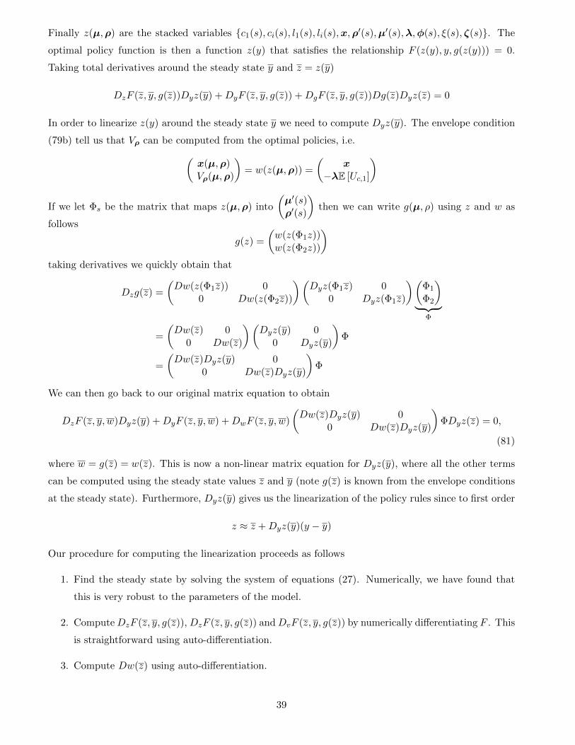
Finally z(µ,ρ) are the stacked variables {c1(s), ci(s), l1(s), li(s),x,ρ′(s),µ′(s),λ,φ(s), ξ(s), ζ(s)}. The

optimal policy function is then a function z(y) that satisfies the relationship F (z(y), y, g(z(y))) = 0.

Taking total derivatives around the steady state y and z = z(y)

DzF (z, y, g(z))Dyz(y) +DyF (z, y, g(z)) +DgF (z, y, g(z))Dg(z)Dyz(z) = 0

In order to linearize z(y) around the steady state y we need to compute Dyz(y). The envelope condition

(79b) tell us that Vρ can be computed from the optimal policies, i.e.(x(µ,ρ)Vρ(µ,ρ)

)= w(z(µ,ρ)) =

(x

−λE [Uc,1]

)

If we let Φs be the matrix that maps z(µ,ρ) into

(µ′(s)ρ′(s)

)then we can write g(µ, ρ) using z and w as

follows

g(z) =

(w(z(Φ1z))w(z(Φ2z))

)taking derivatives we quickly obtain that

Dzg(z) =

(Dw(z(Φ1z)) 0

0 Dw(z(Φ2z))

)(Dyz(Φ1z) 0

0 Dyz(Φ1z)

)(Φ1

Φ2

)︸ ︷︷ ︸

Φ

=

(Dw(z) 0

0 Dw(z)

)(Dyz(y) 0

0 Dyz(y)

)Φ

=

(Dw(z)Dyz(y) 0

0 Dw(z)Dyz(y)

)Φ

We can then go back to our original matrix equation to obtain

DzF (z, y, w)Dyz(y) +DyF (z, y, w) +DwF (z, y, w)

(Dw(z)Dyz(y) 0

0 Dw(z)Dyz(y)

)ΦDyz(z) = 0,

(81)

where w = g(z) = w(z). This is now a non-linear matrix equation for Dyz(y), where all the other terms

can be computed using the steady state values z and y (note g(z) is known from the envelope conditions

at the steady state). Furthermore, Dyz(y) gives us the linearization of the policy rules since to first order

z ≈ z +Dyz(y)(y − y)

Our procedure for computing the linearization proceeds as follows

1. Find the steady state by solving the system of equations (27). Numerically, we have found that

this is very robust to the parameters of the model.

2. ComputeDzF (z, y, g(z)), DzF (z, y, g(z)) andDvF (z, y, g(z)) by numerically differentiating F . This

is straightforward using auto-differentiation.

3. Compute Dw(z) using auto-differentiation.

39

4. Construct a matrix equation as follows. Given policies A = Dw(z)Dyz(y) (these are the linearized

policies of x and Vρ with respect to (µ,ρ)), it is possible to solve for Dyz(y) from

Dyz(z) = −(DzF (z, y, w) +DwF (z, y, w)

(A 00 A

)Φ

)−1

DyF (z, y, w)

We wish to find an A such that

A = Dw(z)Dyz(z)

Given the linearized policy rules it is then possible to evaluate the local stability of the steady state.

We find that in the absence of discount factor shocks the steady state is stable generically across the

parameter space.

This linearization can be used to construct the bordered hessian of the problem (24) at the steady

state. We can then apply second order tests to verify that the first order necessary conditions are

sufficient.

A.6 Proof for Proposition 6

Proof.

The state at time t can be written as

Ψt = BtBt−1 · · ·B1Ψ0.

where the Bi are all random variables being B(s) with probability Pr(s). Taking expectations and

applying independence we then obtain

E0[Ψt] = E0[BtBt−1 · · ·B1]Ψ0 (82)

= E[Bt]E[Bt−1] · E[B1]Ψ0 (83)

= BtΨ0 (84)

where B = EB(s). If eigenvalues of B are positive and strictly less than 1, at least, in expectation the

linearized system converges that is

¯Ψt|0 ≡ E0[Ψt] = B

tΨ0 → 0. (85)

It should be noted that the conditional expectation actually captures a significant portion of the linearized

dynamics. The remaining question is does the distribution converge to 0. This can be done by analyzing

the variance. Let

ΣΨ,t|0 = E0

[(Ψt − ¯

Ψt)(Ψt|0 −¯Ψt|0)′

]or

ΣΨ,t|0 = E0ΨtΨ′t −

¯Ψt|0

¯Ψ′t|0. (86)

Note that if eigenvalues of B are positive and strictly less that 1,¯Ψt|0 converges to 0. Using the indepen-

dence of Ψt−1 and Bt, and Ψt = BtΨt−1, we quickly obtain that for large t

40

ΣΨ,t|0 ≈ E[BΣΨ,t−1|0B′.] (87)

Showing that Ψt|0 → 0 in distribution, amounts to showing that ΣΨ,t|0 → 0 for any starting point ΣΨ

and following the process in equation (87). One can obtain a necessary condition for ‖ΣΨ,t|0‖ → 0 under

the process in equation (87). That process can be rewritten as follows

ΣΨ,t|0 = E[BΣΨ,t−1|0B′] (88)

=∑s

Pr(s)B(s)ΣΨ,t−1|0B(s)′ (89)

=∑s

Pr(s)(B + (B(s)−B))ΣΨ,t−1|0(B + (B(s)−B))′ (90)

= BΣΨ,t−1|0B′+∑s

Pr(s)(B(s)−B)ΣΨ,t−1|0(B(s)−B)′. (91)

This is a deterministic linear system in ΣΨ,t|0. Suppose we reshape ΣΨ,t|0 as a vector (denoted by

vec(ΣΨ,t|0)) and let B be a (square) matrix such that equation 91 is written as

vec(ΣΨ,t|0) = Bvec(ΣΨ,t−1|0).

The stability of this system is guaranteed if the (real part) of eigenvalues of B are less than 1.

41

References

Aiyagari, S. Rao, Albert Marcet, Thomas J. Sargent, and Juha Seppala. 2002. “Optimal

Taxation without State Contingent Debt.” Journal of Political Economy, 110(6): 1220–1254, URL:

http://www.jstor.org/stable/10.1086/343744.

Albanesi, S., and R. Armenter. 2012. “Intertemporal Distortions in the Second Best.” The Review of

Economic Studies, 79(4): 1271–1307, URL: http://restud.oxfordjournals.org/lookup/doi/10.

1093/restud/rds014, DOI: http://dx.doi.org/10.1093/restud/rds014.

Autor, DH, LF Katz, and MS Kearney. 2008. “Trends in US wage inequality: Revising the revision-

ists.” The Review of Economics and Statistics, 90(2): 300–323, URL: http://www.mitpressjournals.

org/doi/abs/10.1162/rest.90.2.300, DOI: http://dx.doi.org/10.1162/rest.90.2.300.

Azzimonti, Marina, Eva de Francisco, and Per Krusell. 2008a. “Aggregation and Aggregation.”

Journal of the European Economic Association, 6(2-3): 381–394, URL: http://doi.wiley.com/10.

1162/JEEA.2008.6.2-3.381, DOI: http://dx.doi.org/10.1162/JEEA.2008.6.2-3.381.

Azzimonti, Marina, Eva de Francisco, and Per Krusell. 2008b. “Production subsidies and redis-

tribution.” Journal of Economic Theory, 142(1): 73–99, URL: http://linkinghub.elsevier.com/

retrieve/pii/S0022053107001020, DOI: http://dx.doi.org/10.1016/j.jet.2007.03.009.

Barro, Robert J. 1974. “Are government bonds net wealth?.” The Journal of Political Economy, 82(6):

1095–1117, URL: http://www.jstor.org/stable/10.2307/1830663.

Barro, Robert J. 1979. “On the determination of the public debt.” The Journal of Political Economy,

87(5): 940–971, URL: http://www.jstor.org/stable/10.2307/1833077.

Bassetto, Marco. 1999. “Optimal Fiscal Policy with Heterogeneous Agents.”

Bassetto, Marco, and Narayana Kocherlakota. 2004. “On the irrelevance of government debt when

taxes are distortionary.” Journal of Monetary Economics, 51(2): 299–304, URL: http://linkinghub.

elsevier.com/retrieve/pii/S0304393203001430, DOI: http://dx.doi.org/10.1016/j.jmoneco.

2002.12.001.

Battaglini, Marco, and Stephen Coate. 2007. “Inefficiency in Legislative Policymaking: A Dynamic

Analysis.” American Economic Review, 97(1): 118–149, URL: http://www.aeaweb.org/articles.

php?doi=10.1257/aer.97.1.118, DOI: http://dx.doi.org/10.1257/aer.97.1.118.

Battaglini, Marco, and Stephen Coate. 2008. “A Dynamic Theory of Public Spending, Taxation,

and Debt.” American Economic Review, 98(1): 201–236, URL: http://www.aeaweb.org/articles.

php?doi=10.1257/aer.98.1.201, DOI: http://dx.doi.org/10.1257/aer.98.1.201.

Bhandari, Anmol, David Evans, Mikhail Golosov, and Thomas Sargent. 2013. “Optimal fiscal

policies in some economies with incomplete asset markets.”

42

Boldrin, Michele, Lawrence J. Christiano, and Jonas DM Fisher. 2001. “Habit Persistence,

Asset Returns, and the Business Cycle.” American Economic Review, 91(1): 149–166, URL: http:

//ideas.repec.org/a/aea/aecrev/v91y2001i1p149-166.html.

Bryant, John, and Neil Wallace. 1984. “A Price Discrimination Analysis of Monetary Policy.” The

Review of Economic Studies, 51(2): , p. 279, URL: http://restud.oxfordjournals.org/lookup/

doi/10.2307/2297692, DOI: http://dx.doi.org/10.2307/2297692.

Chari, V V, Lawrence J Christiano, and Patrick J Kehoe. 1994. “Optimal Fiscal Pol-

icy in a Business Cycle Model.” Journal of Political Economy, 102(4): 617–652, URL: http://

www.nber.org/papers/w4490http://www.jstor.org/stable/2138759, DOI: http://dx.doi.org/

10.2307/2138759.

Constantinides, George, and Darrell Duffie. 1996. “Asset pricing with heterogeneous consumers.”

Journal of Political economy, 104(2): 219–240, URL: http://www.jstor.org/stable/10.2307/

2138925.

Correia, Isabel. 2010. “Consumption taxes and redistribution.” American Economic Review,

100(September): 1673–1694, URL: http://www.ingentaconnect.com/content/aea/aer/2010/

00000100/00000004/art00014.

Faraglia, Elisa, Albert Marcet, and Andrew Scott. 2012. “Dealing with Maturity : Optimal Fiscal

Policy with Long Bonds.”

Farhi, Emmanuel. 2010. “Capital Taxation and Ownership When Markets Are Incomplete.” Journal

of Political Economy, 118(5): 908–948, URL: http://www.jstor.org/stable/10.1086/657996.

Golosov, Mikhail, Aleh Tsyvinski, and Ivan Werning. 2007. “New dynamic public finance: a

user’s guide.” In NBER Macroeconomics Annual 2006, Volume 21. 21: MIT Press, 317–388, URL:

http://www.nber.org/chapters/c11181.pdf.

Guvenen, Fatih, Serdar Ozkan, and Jae Song. 2012. “The Nature of Countercyclical Income Risk.”

Working Paper 18035, National Bureau of Economic Research.

Judd, Kenneth L., Lilia Maliar, and Serguei Maliar. 2011. “Numerically stable and accurate

stochastic simulation approaches for solving dynamic economic models.” Quantitative Economics, 2(2):

173–210, URL: http://doi.wiley.com/10.3982/QE14, DOI: http://dx.doi.org/10.3982/QE14.

Kydland, Finn E, and Edward C Prescott. 1980. “Dynamic optimal taxation, rational expectations

and optimal control.” Journal of Economic Dynamics and Control, 2(0): 79–91, URL: http://www.

sciencedirect.com/science/article/pii/0165188980900524, DOI: http://dx.doi.org/http://

dx.doi.org/10.1016/0165-1889(80)90052-4.

43

Lucas, Robert E, and Nancy L Stokey. 1983. “Optimal fiscal and monetary policy in an economy

without capital.” Journal of Monetary Economics, 12(1): 55–93, URL: http://www.sciencedirect.

com/science/article/pii/0304393283900491, DOI: http://dx.doi.org/http://dx.doi.org/10.

1016/0304-3932(83)90049-1.

Magill, Michael, and Martine Quinzii. 1994. “Infinite Horizon Incomplete Markets.” Economet-

rica, 62(4): 853–880, URL: http://www.jstor.org/stable/2951735, DOI: http://dx.doi.org/10.

2307/2951735.

McKay, Alisdair, and Ricardo Reis. 2013. “The role of automatic stabilizers in the US business

cycle.”Technical report, National Bureau of Economic Research.

Newcomb, Simon. 1865. A critical examination of our financial policy during the Southern rebellion.

Ray, Debraj. 2002. “The Time Structure of Self-Enforcing Agreements.” Econometrica, 70(2): 547–582,

URL: http://onlinelibrary.wiley.com/doi/10.1111/1468-0262.00295/full.

Reinhart, Carmen M, and Kenneth S Rogoff. 2010. “Growth in a Time of Debt.” American

Economic Review, 100(2): 573–578, URL: http://pubs.aeaweb.org/doi/abs/10.1257/aer.100.2.

573, DOI: http://dx.doi.org/10.1257/aer.100.2.573.

Sargent, Thomas J. 1987. Dynamic macroeconomic theory.: Harvard University Press.

Sargent, Thomas J., and Bruce D. Smith. 1987. “Irrelevance of open market operations in some

economies with government currency being dominated in rate of return.” American Economic Review,

77(1): 78–92, URL: http://ideas.repec.org/a/aea/aecrev/v77y1987i1p78-92.html.

Shin, Yongseok. 2006. “Ramsey meets Bewley: Optimal government financing with incomplete mar-

kets.” Unpublished manuscript, Washington University in St. Louis(August): .

Wallace, Neil. 1981. “A Modigliani-Miller Theorem for Open-Market Operations.” The American

Economic Review, 71(3): 267–274, URL: http://www.jstor.org/stable/1802777, DOI: http:

//dx.doi.org/10.2307/1802777.

Werning, Ivan. 2007. “Optimal Fiscal Policy with Redistribution,.” Quarterly Journal of Economics,

122(August): 925–967, URL: http://qje.oxfordjournals.org/content/122/3/925.abstract,

DOI: http://dx.doi.org/10.1162/qjec.122.3.925.

Werning, Ivan. 2012. “Notes on Tax Smoothing with Heterogeneous Agents.”

Yared, Pierre. 2010. “Politicians, Taxes and Debt.” Review of Economic Studies, 77(2): 806–

840, URL: http://restud.oxfordjournals.org/lookup/doi/10.1111/j.1467-937X.2009.00584.

x, DOI: http://dx.doi.org/10.1111/j.1467-937X.2009.00584.x.

44

Yared, Pierre. 2012. “Optimal Fiscal Policy in an Economy with Private Borrowing Limits.” DOI:

http://dx.doi.org/10.1111/jeea.12010.

Yared, Pierre. 2013. “Public Debt Under Limited Private Credit.” Journal of the European Economic

Association, 11(2): 229–245, URL: http://doi.wiley.com/10.1111/jeea.12010, DOI: http://dx.

doi.org/10.1111/jeea.12010.

45

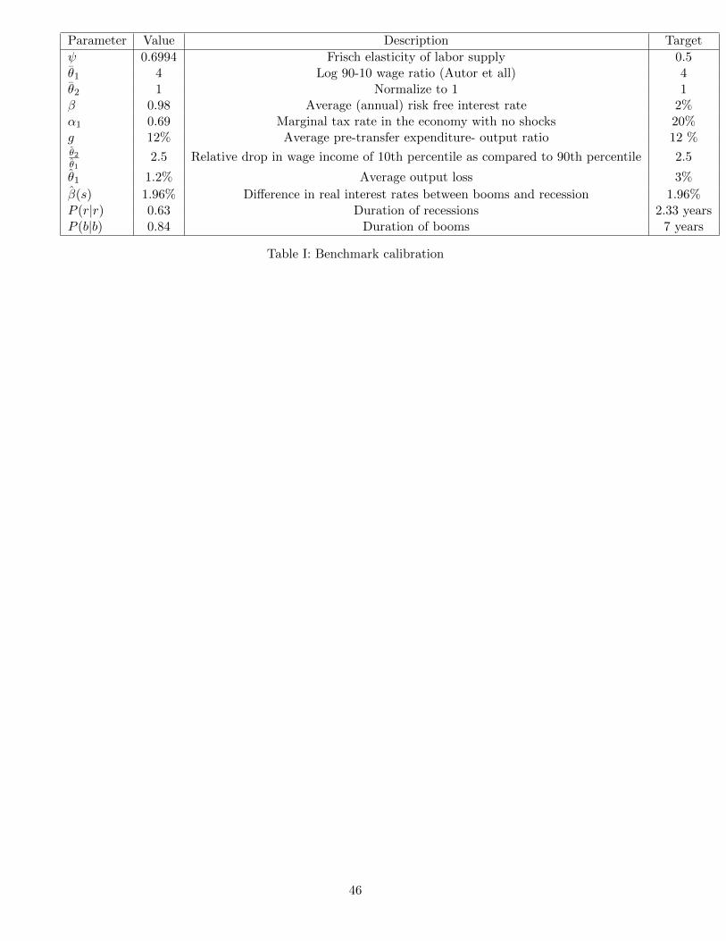
Parameter Value Description Target

ψ 0.6994 Frisch elasticity of labor supply 0.5θ1 4 Log 90-10 wage ratio (Autor et all) 4θ2 1 Normalize to 1 1β 0.98 Average (annual) risk free interest rate 2%α1 0.69 Marginal tax rate in the economy with no shocks 20%g 12% Average pre-transfer expenditure- output ratio 12 %θ2θ1

2.5 Relative drop in wage income of 10th percentile as compared to 90th percentile 2.5

θ1 1.2% Average output loss 3%

β(s) 1.96% Difference in real interest rates between booms and recession 1.96%P (r|r) 0.63 Duration of recessions 2.33 yearsP (b|b) 0.84 Duration of booms 7 years

Table I: Benchmark calibration

46

∆g ∆B ∆T ∆[τθ1l1] ∆[τθ2l2] ∆Y ∆τ

Benchmark 0.0000 -1.1561 0.6871 -0.1593 -0.3096 -2.8536 0.3732

Acyclical Interest Rates 0.0000 -1.1126 0.6591 -0.1497 -0.3038 -2.8613 0.3879

Countercyclical Interest Rates 0.0000 -1.0794 0.6387 -0.1415 -0.2992 -2.8677 0.3997

No Inequality 0.0000 -0.1380 -0.5459 -0.5635 -0.1204 -2.6294 0.0622

Expenditure Shocks -7.5037 2.9137 2.8612 -1.3759 -0.3530 -2.3443 -1.1598

Table II: The tables summarizes the changes in the different components of the government budget as wetransit from “boom” to a “recession”. All numbers are normalized by un-distorted GDP except τ andreported in percentages.

47

Affine approximation to taxes

Figure I: The U.S. tax-transfer system is poorly approximated by a linear function, better by an affinefunction.

48

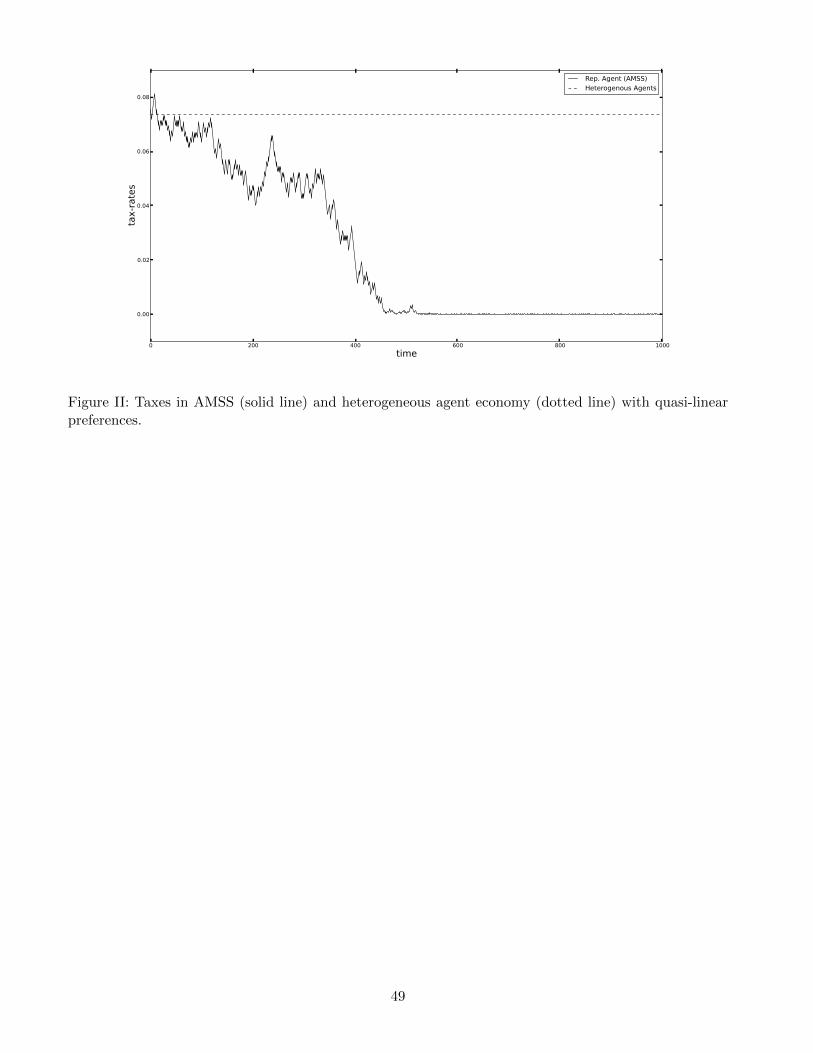
0 200 400 600 800 1000time

0.00

0.02

0.04

0.06

0.08

tax-rates

Rep. Agent (AMSS)Heterogenous Agents

Figure II: Taxes in AMSS (solid line) and heterogeneous agent economy (dotted line) with quasi-linearpreferences.

49

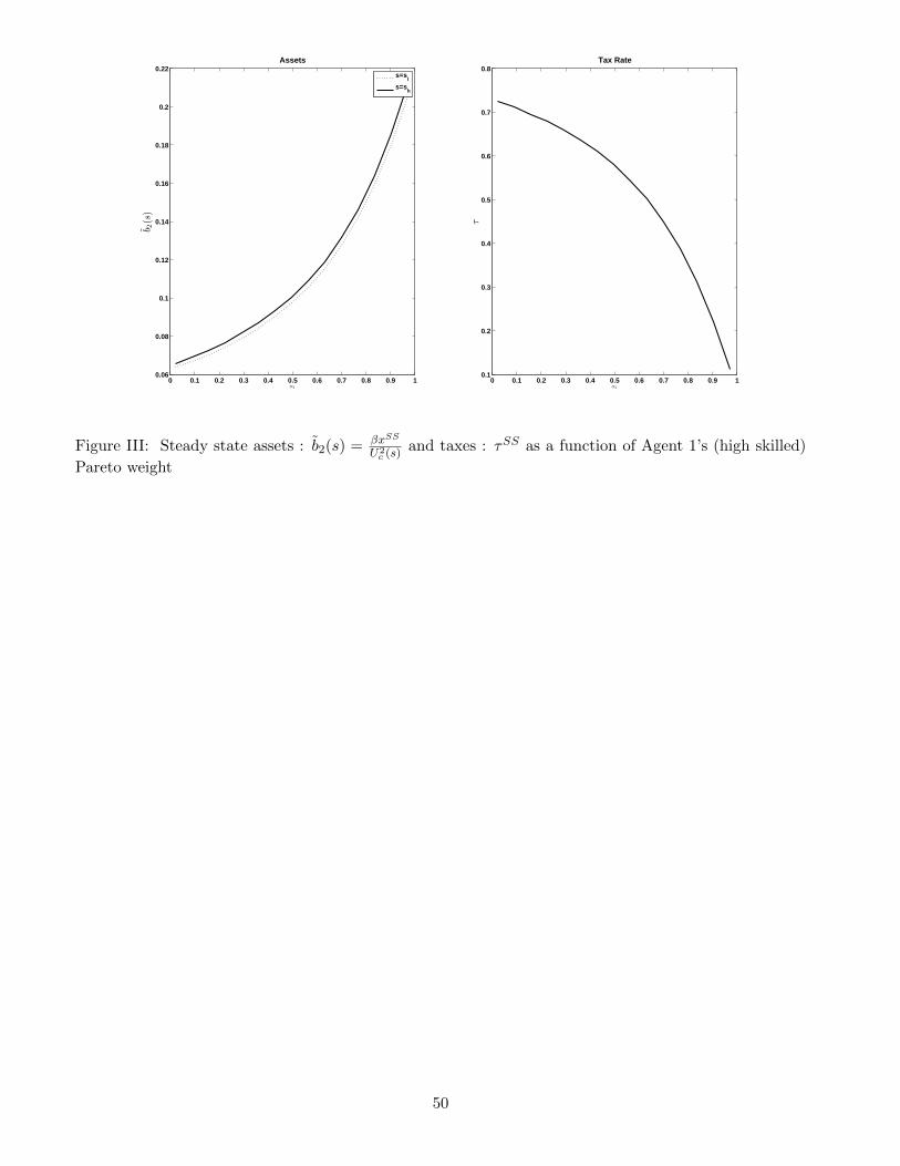
0 0.1 0.2 0.3 0.4 0.5 0.6 0.7 0.8 0.9 10.06

0.08

0.1

0.12

0.14

0.16

0.18

0.2

0.22

α1

b2(s)

Assets

s=s

l

s=sh

0 0.1 0.2 0.3 0.4 0.5 0.6 0.7 0.8 0.9 10.1

0.2

0.3

0.4

0.5

0.6

0.7

0.8

α1

τ

Tax Rate

Figure III: Steady state assets : b2(s) = βxSS

U2c (s)

and taxes : τSS as a function of Agent 1’s (high skilled)

Pareto weight

50

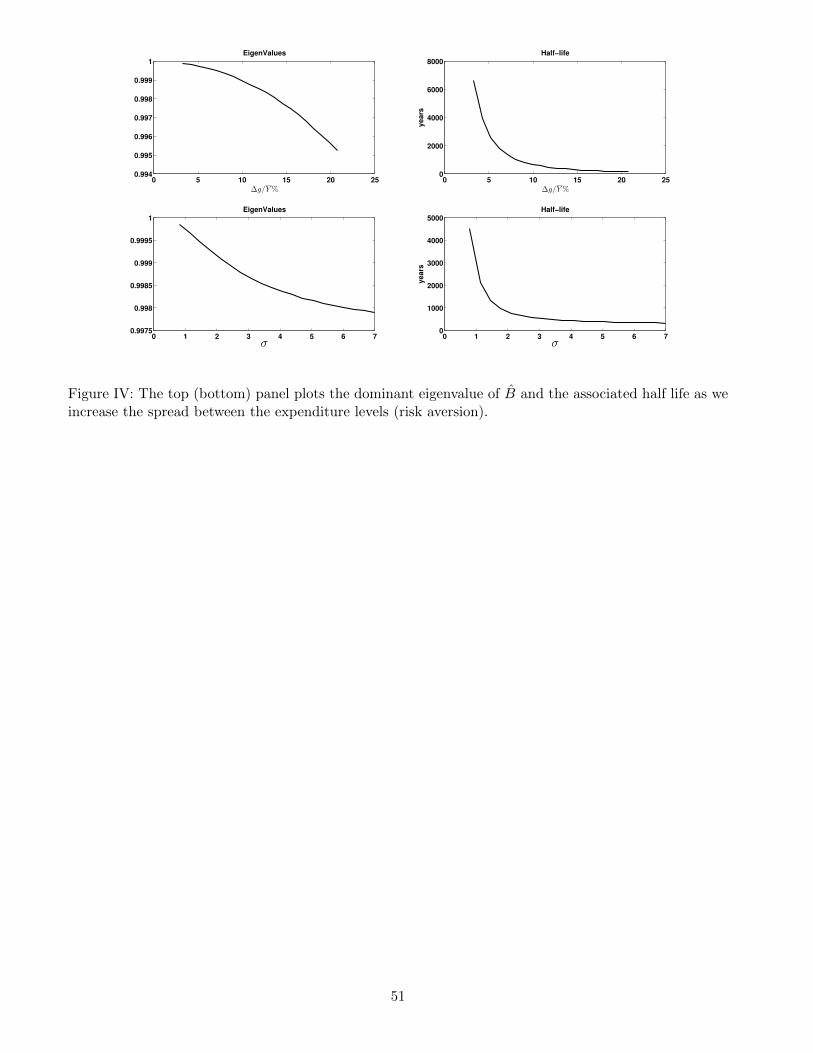
0 5 10 15 20 250.994

0.995

0.996

0.997

0.998

0.999

1

∆g/Y%

EigenValues

0 5 10 15 20 250

2000

4000

6000

8000

∆g/Y%

years

Half−life

0 1 2 3 4 5 6 70.9975

0.998

0.9985

0.999

0.9995

1

σ

EigenValues

0 1 2 3 4 5 6 70

1000

2000

3000

4000

5000

σ

years

Half−life

Figure IV: The top (bottom) panel plots the dominant eigenvalue of B and the associated half life as weincrease the spread between the expenditure levels (risk aversion).

51

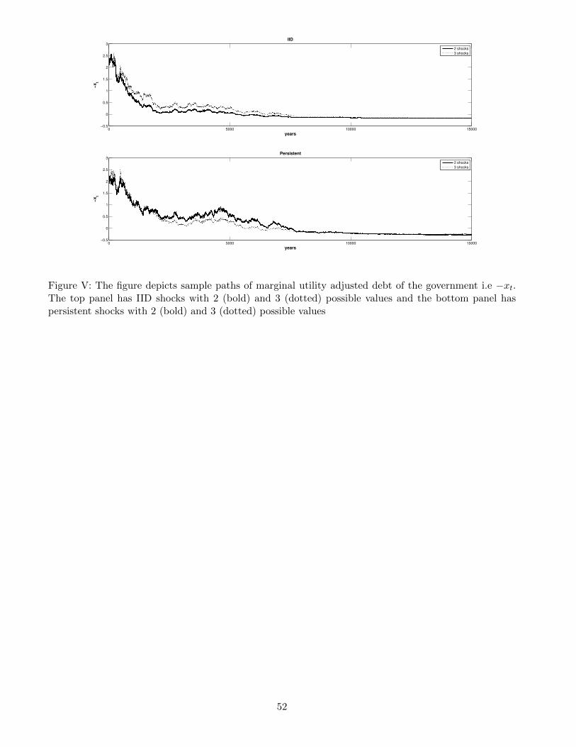
0 5000 10000 15000−0.5

0

0.5

1

1.5

2

2.5

3

years

−xt

IID

2 shocks

3 shocks

0 5000 10000 15000−0.5

0

0.5

1

1.5

2

2.5

3

years

−xt

Persistent

2 shocks

3 shocks

Figure V: The figure depicts sample paths of marginal utility adjusted debt of the government i.e −xt.The top panel has IID shocks with 2 (bold) and 3 (dotted) possible values and the bottom panel haspersistent shocks with 2 (bold) and 3 (dotted) possible values

52

0 500 1000 1500 2000 2500 3000 3500 4000 4500 5000−0.8

−0.6

−0.4

−0.2

0

0.2

0.4

0.6

0.8

years

Debt−Gdp

Figure VI: Debt benchmark (o), acyclical interest rates (+), countercyclical interest rates (�) and noinequality shocks (�)

53

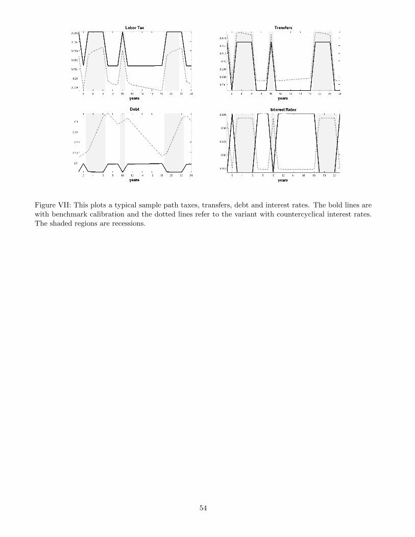
Figure VII: This plots a typical sample path taxes, transfers, debt and interest rates. The bold lines arewith benchmark calibration and the dotted lines refer to the variant with countercyclical interest rates.The shaded regions are recessions.

54

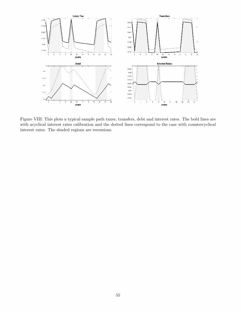
Figure VIII: This plots a typical sample path taxes, transfers, debt and interest rates. The bold lines arewith acyclical interest rates calibration and the dotted lines correspond to the case with countercyclicalinterest rates. The shaded regions are recessions.

55