TAX-SPEND DEBATE: EMPIRICAL EVIDENCE FROM … · address the budget disequilibrium and bring the...

* Assistant Professor, School of Business, Lovely Professional University, Delhi- Jalandhar NH-1,Phagwara, Punjab, India-144411, E-mail: [email protected]

TAX-SPEND DEBATE: EMPIRICAL EVIDENCE FROMUTTAR PRADESH, INDIA

Anubhav Singh*

Abstract: The continuously mounting Debt-GDP ratio in most of Indian states had made themrealize that a ponzi game cannot be played for long. A viable solution to curb the growing debts,address the budget disequilibrium and bring the budgetary figures in Line with FRBM Act is tomake either expenditure or revenues as target variable. To meet these legislative requirements forfiscal prudence policy makers are often confronted with the dilemma of either changing expendituresor revenues because different hypotheses-”Tax-and-Spend”, “Spend-and-Tax” and “FiscalSynchronization” in economic literature suggest different policy prescriptions for curbing themounting Debts. This paper empirically tries to find out right policy measure for Uttar Pradeshgovernment using time series data over the period 1980-81 to 2012-13. Augmented Dicky Fuller(ADF) test along with Phillip Perron(PP) test was used to establish the order of integration;Engel-Yoro three step method was used for examining cointergration and estimating long runcoefficients. Further, modified Granger causality test confirmed the causality from revenues toexpenditures thereby confirming to Friedman’s version of ‘Tax-and-Spend’ hypothesis. Studysuggest increasing the taxes as a measure to reduce debt state will not yield anything desirable,instead it will further push up the expenditures. Instead government should try for reducingexpenditures or decreasing taxes that inturn will cause a decrease in expenditures.

Key Words:Cointegration, Engel-Yoo,Fiscal Deficit, Synchronisation, Tax-and–SpendHypothesis

JEL Classification:H2, C22

A) INTRODUCTION

Contemporary economies both at center and state levels are plagued with hugeand escalating budget deficits. The adverse consequences of these mounting deficitsare manifested in form of higher interest rates, slow capital formation and highunemployment rates which turn still more adverse once this debt is financedthrough issuance of government bonds or seigniorage. In such a situation anapposite fiscal policy has a vital role in mitigating short run fluctuations in outputand employment by bringing the economy closer to potential output (Zagler andDurnecker, 2003). But any such policy aiming at fiscal correction is contingent onGovernment expenditure Allocations and Revenue collections. As such

I J A B E R, Vol. 14, No. 3, (2016): 2269-2285

2270 � Anubhav Singh

understanding the nexus between government revenues and expenditures hadassumed significant importance for a sound fiscal policy that could promote pricestability and sustain growth in output and employment. Understanding the natureof relationship between expenditures and revenues can guide us towardsappropriate policy prescription to rein in the mounting debt and associatedeconomic ills. If the nature of relationship suggests that there exists a long runequilibrium relationship between government revenue and governmentexpenditures and former causes latter, budget deficit can be eliminated bycontrolling revenues and not by increasing the revenues which will further increasethe expenditure and worsen debt situation. However, if expenditures causerevenues; such a Behaviour can induce capital outflow due to fear of paying highertaxes in future. In such a situation government must aim at curtailing theexpenditures for desired results. Present study aims at finding a correct policydecision at sub national level by taking data from Uttar Pradesh economy. BecauseUttar Pradesh like many other Indian states is grabbling with the mounting debtproblem. Payne (1998) remarked that many state operate under legislative orconstitutional requirements which attempt to constrain deficits.U.P governmenthas also passed Fiscal Responsibility and Budget Management Act (FRBM) inFebruary 2004 thereby imposing a legislative binding for bringing about fiscalconsolidation in state by curbing the growing fiscal deficit (7.33% of GSDP in 2003-04)and mounting Debt-GSDP (46% of GSDP in 2003-04) ratio of the state government.The Act also envisaged bringing down the revenue deficit to Zero and Fiscal Deficit-GSDP ratio to below 3% by the end of March 2009. Target for total governmentliabilities as percentage of GSDP was set at 25% to be achieved by March 2018.However, a lot is yet to be done in this line when we see the actual performance ofstate. The total outstanding liabilities of U.P government as percentage of GSDP arepersistently more than 30 percent (38 and 36.3 percent’s during 2011-12 and 2012-13respectively).Gross Fiscal deficit (GFD) as percentage of GSDP for 2011-12 and 2012-13 was 2.3 and 2.8 respectively while average figures for all non-special categorystates during these years were 2.2% and 2.6% respectively. The debt burden couldbetter be understood from the fact that during 2010-11 and 2012-13 interest paymentsas percentage of Revenue expenditure stood at 12.5 and 10.9 percent respectively.To arrive at a rational policy Prescription for U.P we undertake this empirical exercise.The balance of this paper is organized as: Section B.1 contains review of theoreticalliterature while empirical literature is presented separately in section B.2. In sectionC Methodology and empirical analysis is presented under different subheadings.Paper ends with conclusion and policy implications given in section D.

B.1) Theoretical Literature Review

The literature in economics has so far identified four alternative hypotheses thatcharacterise the dynamic relationship between revenues and governmentexpenditures. A brief account of these alternative hypotheses is presented below.

Tax-Spend Debate: Empirical Evidence from Uttar Pradesh, India � 2271

Tax-and-Spend hypothesis: The Tax-and-Spend school championed byFriedman views expenditure as adjusting, up or down to whatever level can besupported by revenues. Friedman (1978, 82), Ram (1988) as well as Buchanan andWagner (1977, 1978) advocate such view. According to Friedman level of spendingadjusts to the level of tax available, as such causality runs from tax to expenditure.However, he did not advocate raising taxes to bring down deficits as he opinedthat former will invite more spending . Friedman (1982) explains:

“You can not reduce the deficit by raising the taxes. Increasing taxes only results in morespending, leaving the deficit at the highest level conceivably accepted by the public. Politicalrule number one is government spends what government receives plus as much more as itcan get away with.”

Because of this positive causal relationship Friedman had long proposed tax cutsas a means of reducing budget deficits. He reasoned that tax cuts will lead to largerdeficits which in turn will exert a mounting pressure on the governments to curtailits expenditures. Buchanan and Wagner supported same causal direction , butunlike Friedman they hypothesise a negative relationship wherein a decrease ingovernment revenues will lead to an increase in government expenditures andvice versa. Buchanan and Wagner opined that high public deficits have beenresponsible for growth of public spending, and if that spending is to be financedby direct taxes ,people would have asked for decrease in public spending Theyargue that tax payers suffer from fiscal illusion as any reduction in taxes is perceivedby them as a reduction in cost of public programmes ( low price for public goodsand services ) and they start demanding increasing quantities. However publicincurs even higher costs primarily because of indirect inflation taxation which is aconsequence of excessive money creation. Also government debt financing willlead to high interest rates that may crowd out private investment . Thus tax cut inconjunction with resultant government spending would actually lead to higherspending and higher deficits. Following this reasoning Buchanan and Wagneradvocate a tax increase that will be perceived as higher costs for government goodsand services by tax payers , as a policy prescription for bringing down the budgetdeficit. Although these two views differ with regard to policy their policyprescription for bringing down the deficit both support causality from tax revenuesto spending. for this reason it is also known as “Revenue Dominance hypothesis”(Hansan and Lincolon;s1997).to determine empirically the validity of thishypothesis unidirectional causality should stem from government revenues togovernment expenditures.

i) Spend-and-Tax Hypothesis: According to this hypothesis government firstfixes its expenditure programme and then adjusts its tax and revenue policy toaccommodate the desired spending. As such increased taxes and borrowing arisesbecause of increased government spending. This view is more pro-Keynesian andis supported by Wiseman and Peacock (1979) and Barro’s (1979) Tax –smoothing


model. Wiseman and Peacock argue that a temporary increase in governmentspending (due to emergency purposes) leads to increase in government taxes andother types of revenues that tend to become enduring in due course of time andfinally assume permanent nature. They are of the view that severe crisis that initiallyforce up the government expenditure, more than taxes, is capable of changingpublic attitude about proper size of government. Narayan (2005) in this contextremarks that the original tax increase due to crises becomes a permanent featurein tax policies .in empirical sense this implies that causality runs from expendituresto tax. Barro, supporting the same causal direction uses Ricardian view to justifythis hypothesis. He argues that an increased expenditure arranged through higherborrowings now results in increase in expected future taxes. With this perceptionof higher future tax liability tax payers decrease present spending to pay futuretaxes. Both these arguments establish that expenditure changes precede changesin taxation level. Under this causality pattern the optimal solution to control thebudget deficit obviously is the expenditure cuts. Validity of this hypothesis isestablished if unidirectional causality stems from government expenditures togovernment revenues.

ii) Fiscal Synchronisation Hypothesis: This hypothesis postulates thatdecisions regarding tax and expenditures are taken simultaneously as such causalityruns in both the directions. Musgrave (1966), and Meltzer and Richard (1981)advocate this view. According to Metzler and Richard quantity and quality ofpublic goods reflect the preferences of a community and size of government isdetermined by welfare maximizing choice of decisive individuals. publicsimultaneously determines the levels of government spending and taxation bycontrasting the benefits of public goods with their costs. According to Musgravethe expenditure and tax sides of government must be decided jointly so as tomaximize society’s inter temporal social welfare function. This view is also in linewith Wildavsky (1964) incremental budgetary process wherein the expendituresand revenues change concurrently on incremental basis. Joint determination assuch implies that one has influence on other .For empirical verification of thishypothesis bi-directional causality should be proved.

iii) Institutional Separation Hypothesis (Fiscal Neutrality): This hypothesiswhich is in opposite to Fiscal Synchronization view is supported by Hoover andSheffrin (1992) and Baghestani and McNown (1994) suggests independence ofrevenues and expenditures because of laws and institutions governing thebudgetary process. According to this hypothesis both legislative and executivebranches of government participate in budgetary process ,but lack of agreementbetween these two independent decision making branches makes revenues andexpenditures independent of each other. Hoover and Sheffrin attribute absence ofcausal link to many important actors with divergent views and interests, whilePearson (2000) attributes it to disagreement between parties or groups in the


decision making process. This view was verified by experience of US economywhere institutional separation of allocation and taxation functions of governmentexists. For example, despite the reform of budget process attempted in congressionalbudget and Impoundment Control Act of 1974 large budgetary deficits persistedin post -1974 period reflecting continued absence of coordination betweenexpenditure and revenue decisions. The Gram-Rudman-Holdings Act was anotherattempt to coordinate the revenue and expenditure decisions of government, whichagain failed to achieve a balanced linkage between two budget components. Hooverand Sheffrin attributed this failure to interplay of numerous diverse interests inthe context of non parliamentary US institutions. In Indian context this can beexplained in terms of FRBM Act 2004.

B.2) Empirical Literature Review

For about past three decades , many studies- using concept of cointegration,Granger causality, parametric and non parametric tests, Asymmetric ECM andother econometric techniques, focused on many countries using data for differenttime periods. These empirical analysis have furnished mixed results and alsocontroversial in case of certain countries including USA. These results differ bothin terms of direction of causality and in terms of short run verses long run natureof relationship between revenues and expenditures for sate and centralgovernments. A brief summary of some of empirical analysis already done in thiscontext is presented below.

A seminal research paper by Anderson, Wallace and Warner (1986) using aVAR model on annual post-world war II data of US economy found empiricalevidence in favour of ‘Spend-and-Tax’ hypothesis which is in sharp contrast withFriedman’s hypothesis that increase in revenue causes increase in expenditures.The data also had not any support for Buchanan and Wagner’s view that highertaxes lead to less government spending. This paper also finds little support forWiseman- Peacock hypothesis that instability leads to growth in governmentexpenditures or revenues. Further, evidence for inflation causing increase in realgovernment expenditure is also weak. Extending the sample period back to 1929,and using only a dummy variable to capture the macroeconomic effects Manageand Marlow reverse the conclusion of Anderson et al. as they found out that eitherthere exists unidirectional causality from revenues to expenditures or bidirectionalcausality depending upon the number of lags in the VAR. In the wake of theseconflicting results Ram (1988) used both long period annual data (1929-83) andshorter period quarterly data (1947-83) and produced results largely consistentwith Manage and Marlow (1986) with causality running from revenues toexpenditures and some feedback following world war second. However, resultsalso showed some evidence for causality running from expenditures to revenuesbut only in case of state and local level governments. Since, study does not involve


use of macroeconomic controls it could not outrightly reject the Anderson et al.conclusion. A study involving analysis in this regard at sub national level alsowas conducted by Miller and Russek (1990) which shows different results in caseof US economy which are in contradiction with earlier studies of Anderson et al.(1986) and Ram (1988). Their results support bidirectional causality between taxesand expenditures (both in nominal and Real terms) for federal, state and locallevel of governments.

Blackley (1986) used long term annual data and found causality running fromrevenues to expenditures. When GNP was introduced as a control variable hefound block causality from GNP and revenues to expenditures but could notestablish significant individual effect of either revenues or GNP on expenditures.He also found significant contemporaneous relationship between GNP changesand revenue changes, but no lagged effects. These results again demonstrate thesensitivity of causality to the inclusion of macroeconomic control variables therebyleaving open the possibility of GNP changes being the driving force behindbudgetary changes.

Ahiakpor and Amirkhalkhali (1989) carried out their study using Canadiandata and their statistical analysis appears to support the claim that raising taxeswould only partially reduce the deficits and will not reduce the expenditures inlong run. They opined for reduction in spending or fiscal restraint rather thanfinding ways of raising additional revenues from taxes.

Payne (1997) also used Canadian data to explore direction of causality butmade use of GDP as additional control variable. He finds out that Revenues followa time path which is independent of both expenditures and GDP. Howeverexpenditures respond to budgetary disequilibrium since budget imbalances appearto be corrected by expenditure changes. Moreover this paper finds that expenditurevariations also respond to GDP ones.

In a study of OECD countries , Joulfaian and Mookerjee (1991) find support for‘Tax-and-Spend’ hypothesis in Italy and Canada; for ‘Spend-and –Tax’ hypothesisin case of US, Japan, Germany, France, United Kingdom, Austria, Finland andGreece and for Fiscal Synchronisation hypothesis in case of Ireland.

Hasan and Lincoln (1997) using Quarterly data for UK and applying Johansenmaximum likelihood procedure found long run equilibrium relationship betweengrowth rates of tax revenue and government spending. The sequential testingprocedure indicates presence of bidirectional causality between tax revenues andgovernment spending. Results of the paper broadly confirm Wildavsky’s incrementalbudgetary theory (Wildavsky, 1964) and empirically accord well with Owoye (1995).

In a wider multinational study by Chang et al. (2002) mixed results wereobtained regarding the dynamics of expenditure –revenue nexus. Grange causality


tests suggest unidirectional causality running from Revenues to spending in caseof Japan, south-Korea, Taiwan, United Kingdom and United States, therebysupporting “Tax-and-Spend’ hypothesis. The reverse causality, supporting ‘Spend-and -Tax’ hypothesis was found in case of Australia and South Africa. In case ofCanada, study found a feedback mechanism between revenues and expendituresthus supporting “Fiscal Synchronisation” hypothesis. For Newzeland and Thailanddirection of causality could not be established in any direction thereby supportinginstitutional separation hypothesis.

Narayan (2005) studied long run relationship between governmentexpenditures and revenues and for nine Asian countries. He found support for‘Tax-and-Spend hypothesis for Indonesia, Singapore, and Srilanka in the shortrun and for Nepal both in short and long run. Study reported evidence of neutralityfor other countries like India, Malaysia, Pakistan, Philippines and Thailand. Hisresults reveal that there is neither a strong support for Tax-and –Spend Hypothesisnor for Spend-and -Tax hypothesis as mixed results are obtained in case of differentcountries.

Narayan and Narayan (2006) found support for the Tax-and Spend hypothesisfor Mauritius, El Salvador, Haiti, Chile and Venezuela.

C) METHODOLOGY AND EMPIRICAL ANALYSIS

This section, for exposition motives, presents methodology applied along withthe results pertaining to present study, under different sub headings:

C.1) Variables and Data sources

Since the study aims at studying the nexus between expenditures and revenuesat sub national level the two variables under consideration are U.P government’sown revenues (R) and expenditures (E). Own revenues (R) include own taxrevenues and own non tax revenues which state govt. can increase or decreaseat state level. Own tax revenues inturn comprise of taxes on commodities andservices, taxes on property and capital transactions, and taxes on agriculturalincome, professions, trade, calling and employment. Non tax revenues mainlycomprise of interest receipts, dividends and profits and receipts from general,social and economic services. Expenditures include revenue (Both Plan and nonplan components) and capital (Development and non development) expendituresexcluding expenditures on public accounts. Data for related variables iscollected from “ State Finances: a study of Budgets”, “Handbook of Statisticson State Government Finances -2004 and 2010 volumes” both published byReserve Bank of India ,and U.P State budgets (various issues). Both the variablesare taken in logarithm form (LR and LE) to avoid the problem ofheteroscedasticity.


C.2) Unit Root Tests

The very first step involved in this empirical analysis of time series data is toascertain the nature of data (Stationary or non stationary). For this, as a preliminarywe take the graphic view of two series. From the graphs [fig. 1.1and fig. 1.2] it isclear that two series ,at levels , are not maintaining a constant mean and seem tofollow an upward trend. However, first differences of both fluctuate around non-zero mean [fig. 1.3 and fig. 1.4].

6

7

8

9

10

11

12

5 10 15 20 25 30

LR

level form

7

8

9

10

11

12

13

5 10 15 20 25 30

LE

le ve l form

-.08

-.04

.00

.04

.08

.12

.16

.20

.24

.28

.32

5 10 15 20 25 30

DLR

first difference

-.08

-.04

.00

.04

.08

.12

.16

.20

.24

.28

.32

5 10 15 20 25 30

DLR

fi rs t differ ence

Figure 1.1 Figure 1.2

Figure 1.3 Figure 1.4

This gives an indication for presence of unit root in level forms and stationarityof first differences of variables. To further verify this we make use of AugmentedDicky Fuller (ADF) and Phillip Perron (PP)tests .The (ADF) test is based uponanalysis of following three different forms of regression for two variables underconsideration. The three forms are

With Drift:


(C.1)

(C.2)

With constant and trend:

(C.3)

(C.4)

Without drift and trend:

(C.5)

(C.6)

In all the three cases hypothesis is

Null; Ho: �3 = 0 ( Unit root is present or series is non stationary )

Alternate: H1: �3 < 0 ( No unit root)

Decision rule :

1) If computed � statistic is more negative than ADF critical values reject Hoimplying series is stationary.

2) If computed statistic is not more negative than ADF critical values acceptHo implying that series is non stationary.

Having obtained these results same test is applied on first differences of twovariables labeled as DLE (�LE) and DLR (�LE). To check their stationarity theregressions equations to be estimated will be as

(C.7)

(C.8)

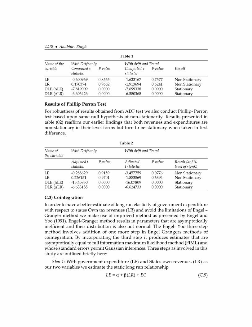
With this back ground of ADF test we below present the test results in Tablefor four variables. In Addition to ADF statistics , for robustness of results, we alsopresent results as per Phillip Perron test for same set of variables. Further followingC. Hill et al. (2008) we present results for equations with drift and/or trend only asthe series does not fluctuate around zero mean. It is because of this we h rule outthe possibility of no trend and drift option. from table (01) it is clear that nullhypothesis of non stationarity could not be rejected at 5% level of significance incase of both the variables but for DLE and DLR null hypothesis of non stationarityis rejected as such both the variables (Revenues and Expenditures) are integratedof order one.


Table 1

Name of the With Drift only With drift and Trendvariable Computed � P value Computed � P value Result

statistic statistic

LE -0.600969 0.8555 -1.623167 0.7577 Non StationaryLR 0.170374 0.9662 -1.913694 0.6241 Non StationaryDLE (�LE) -7.819009 0.0000 -7.699338 0.0000 StationaryDLR (�LR) -6.603426 0.0000 -6.580368 0.0000 Stationary

Results of Phillip Perron Test

For robustness of results obtained from ADF test we also conduct Phillip- Perrontest based upon same null hypothesis of non-stationarity. Results presented intable (02) reaffirm our earlier findings that both revenues and expenditures arenon stationary in their level forms but turn to be stationary when taken in firstdifference.

Table 2

Name of With Drift only With drift and Trendthe variable

Adjusted t P value Adjusted P value Result (at 5%statistic t statistic level of signf.)

LE -0.288629 0.9159 -3.457759 0.0776 Non StationaryLR 0.226151 0.9701 -1.883869 0.6394 Non StationaryDLE (�LE) -15.45830 0.0000 -16.07809 0.0000 StationaryDLR (�LR) -6.633185 0.0000 -6.624733 0.0000 Stationary

C.3) Cointegration

In order to have a better estimate of long run elasticity of government expenditurewith respect to states Own tax revenues (LR) and avoid the limitations of Engel –Granger method we make use of improved method as presented by Engel andYoo (1991). Engel-Granger method results in parameters that are asymptoticallyinefficient and their distribution is also not normal. The Engel- Yoo three stepmethod involves addition of one more step in Engel Grangers methods ofcointegration. By incorporating the third step it produces estimates that areasymptotically equal to full information maximum likelihood method (FIML) andwhose standard errors permit Gaussian inferences. Three steps as involved in thisstudy are outlined briefly here:

Step 1: With government expenditure (LE) and States own revenues (LR) asour two variables we estimate the static long run relationship

LE = � + �(LR) + EC (C.9)


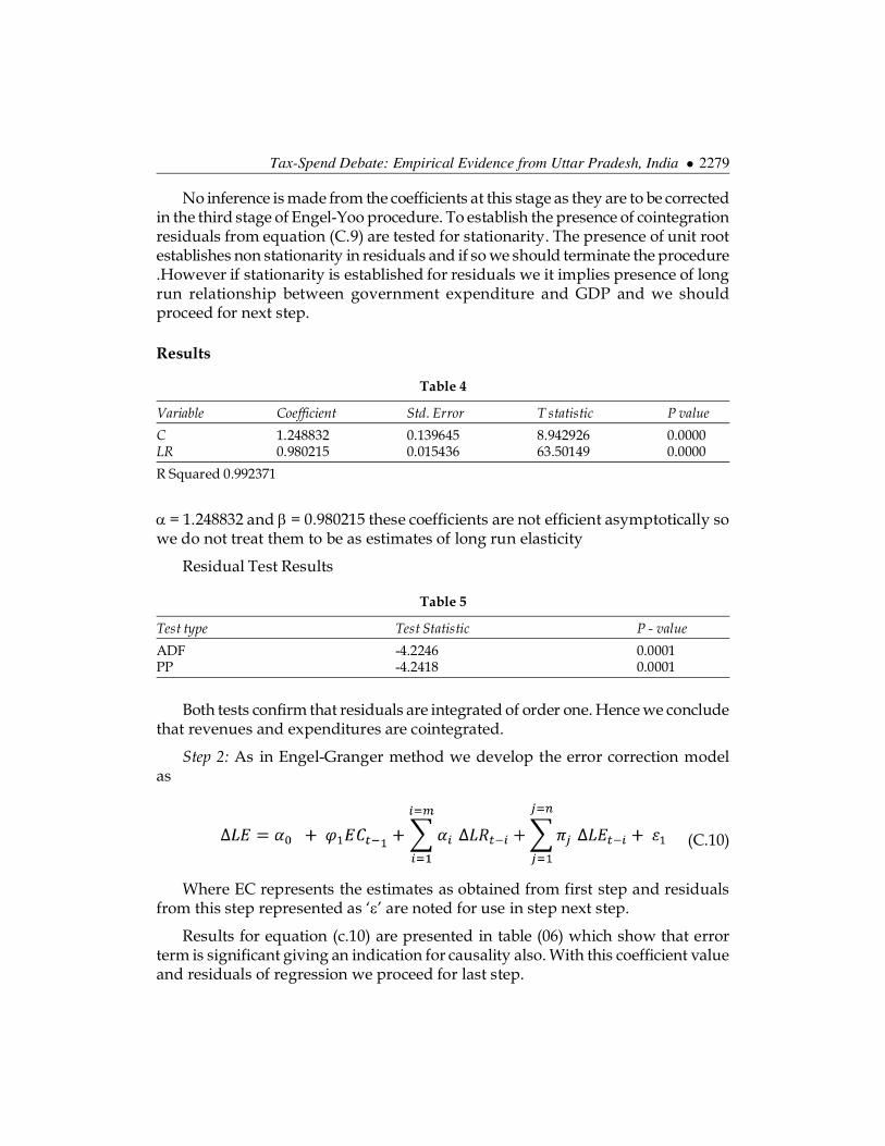
No inference is made from the coefficients at this stage as they are to be correctedin the third stage of Engel-Yoo procedure. To establish the presence of cointegrationresiduals from equation (C.9) are tested for stationarity. The presence of unit rootestablishes non stationarity in residuals and if so we should terminate the procedure.However if stationarity is established for residuals we it implies presence of longrun relationship between government expenditure and GDP and we shouldproceed for next step.

Results

Table 4

Variable Coefficient Std. Error T statistic P value

C 1.248832 0.139645 8.942926 0.0000LR 0.980215 0.015436 63.50149 0.0000

R Squared 0.992371

� = 1.248832 and � = 0.980215 these coefficients are not efficient asymptotically sowe do not treat them to be as estimates of long run elasticity

Residual Test Results

Table 5

Test type Test Statistic P - value

ADF -4.2246 0.0001PP -4.2418 0.0001

Both tests confirm that residuals are integrated of order one. Hence we concludethat revenues and expenditures are cointegrated.

Step 2: As in Engel-Granger method we develop the error correction modelas

(C.10)

Where EC represents the estimates as obtained from first step and residualsfrom this step represented as ‘�’ are noted for use in step next step.

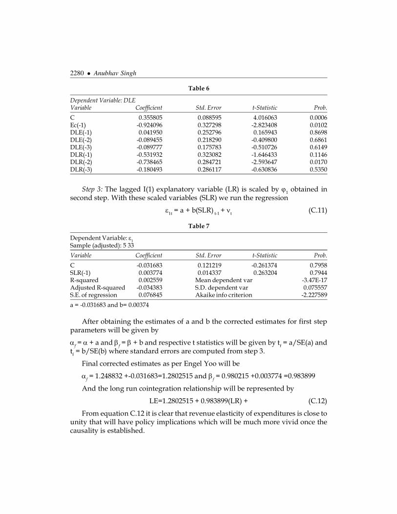
Results for equation (c.10) are presented in table (06) which show that errorterm is significant giving an indication for causality also. With this coefficient valueand residuals of regression we proceed for last step.


Step 3: The lagged I(1) explanatory variable (LR) is scaled by �1 obtained insecond step. With these scaled variables (SLR) we run the regression

�1t = a + b(SLR) t-1 + �t (C.11)

Table 7

Dependent Variable: �1

Sample (adjusted): 5 33

Variable Coefficient Std. Error t-Statistic Prob.

C -0.031683 0.121219 -0.261374 0.7958SLR(-1) 0.003774 0.014337 0.263204 0.7944R-squared 0.002559 Mean dependent var -3.47E-17Adjusted R-squared -0.034383 S.D. dependent var 0.075557S.E. of regression 0.076845 Akaike info criterion -2.227589

a = -0.031683 and b= 0.00374

After obtaining the estimates of a and b the corrected estimates for first stepparameters will be given by

�f = � + a and �f = � + b and respective t statistics will be given by tf = a/SE(a) andtf = b/SE(b) where standard errors are computed from step 3.

Final corrected estimates as per Engel Yoo will be

�f = 1.248832 +-0.031683=1.2802515 and �f = 0.980215 +0.003774 =0.983899

And the long run cointegration relationship will be represented by

LE=1.2802515 + 0.983899(LR) + (C.12)

From equation C.12 it is clear that revenue elasticity of expenditures is close tounity that will have policy implications which will be much more vivid once thecausality is established.

Table 6

Dependent Variable: DLEVariable Coefficient Std. Error t-Statistic Prob.

C 0.355805 0.088595 4.016063 0.0006Ec(-1) -0.924096 0.327298 -2.823408 0.0102DLE(-1) 0.041950 0.252796 0.165943 0.8698DLE(-2) -0.089455 0.218290 -0.409800 0.6861DLE(-3) -0.089777 0.175783 -0.510726 0.6149DLR(-1) -0.531932 0.323082 -1.646433 0.1146DLR(-2) -0.738465 0.284721 -2.593647 0.0170DLR(-3) -0.180493 0.286117 -0.630836 0.5350


C.4) Bi-Variate Granger Causality

For conducting the granger causality test we must have stationary variables. sincewe have shown that LE and LR are non stationary at levels but stationary at firstdifference and also cointegration has been established then following the Grangerrepresentation theorem, either LE must cause LR or LR must cause LE. Sinceimportant assumption of stationarity is not valid here we make use of extendedgranger causality test involving Error correction mechanism. For this we estimate

(C. 13)

Where U1t–1 is the lagged residual term from the cointegration regression;

which is nothing but the error correction term (because two variables arecointegrated). So there are now two sources of causation for LE : (1) through thelagged values of LR and/or (02) through the lagged value of cointegrating vector(i.e. the EC term). The standard Granger Causality test neglects the latter source ofcausation. The null hypothesis of no cointegration implies �1 = �2 = �3 ... ... = �q = �= 0. This can be rejected even if all �‘s are zero but coefficient of lagged EC term isnon zero. This is because EC term includes the impact of TR. To test this hypothesisof no causality we use F test as:

1) Estimate equation (C.11) by OLS and obtain the residual sum of squaresfrom this regression (RSSur).

2) Re –estimate equation dropping all the lagged terms of TR and EC term .obtain the residual sum of Squares (RSSr) from this reduced regression .

Compute the F statistic as

with m and (n-K) degrees of freedom.

Where m is the number of restrictions imposed, k is number of parameterestimated in unrestricted regression and n is the sample size.

If computed value of F exceeds the critical value of F (for specified degrees offreedom) then we reject the null hypothesis of �1 = �2 = �3 ... ... = �q = � = 0. In otherwords we accept that TR is caused either by lagged values of TE or EC term orboth. Same procedure is repeated for the an equation containing variables in reverseorder to test causality direction in reverse order. Results for two Directions ofcausality are presented below

i) LR does not granger cause LE

Residuals were obtained from cointegration equation


(C.14)

And following equation was estimated the following equation.

(C.15)

Since we are dealing with annual data we have used only one lag.However, higher lags were also tested and results remained unaltered.After applying necessary restrictions through Wald test following results wereobtained

Table 8

Test statistic Value d.f Probability

F statistic 5.46447 (2, 27) 0.0101Chi square 10.9289 2 0.0042

From result table it is clear that null hypothesis of Revenuesdoes not Grangercause expenditures is rejected both by F and Chi-Square statistic or to be simpleresults support the Tax-and-Spend hypothesis .

ii) LE does not Granger cause LR

For checking this direction of causality we obtain residuals for the cointegrationequation

(C.15)

Then we estimate the unrestricted equation

(C.16)

and applying Wald test with restrictions we have following results.

Table 9

Test statistic value d.f Probability

F statistic 0.522458 (2, 27) 0.5989Chi square 1.044916 2 0.5931

From results given in table (09), the null hypothesis of expenditures does notgranger cause revenues cannot be rejected and we infer that empirical results dofavour Spend-and-Tax hypothesis.

Hence from bi directional Grager causality test we conclude that behaviour ofU.P Economy supports ‘Spend-and-Tax’ hypothesis thereby confirming toFriedmans view and in accordance with the empirical results found earlier by


D) CONCLUSION AND POLICY IMPLICATIONS

In this study causal nexus between government Revenues and Expenditures hasbeen studied using annual data of Uttar Pradesh for the time period 1980-81 to2012-13. We test four alternative hypotheses- first, Tax and Spend hypothesis;second, Spend and tax hypothesis; third, fiscal synchronization hypothesis andfourth, institutional separation hypothesis. In the empirical exercise ADF test wasused to check the stationarity of variables, modified Engel-granger andCointegration Regression Durbin Watson tests were used to examine long runEquilibrium relationship between two variables and Error correction model wasused to analyse the reconciliation of long run and short run behaviour of twovariables. Further, Engel granger test for Non stationary series was used to examinethe direction of causality . Empirical analysis revealed that there exists a long runequilibrium relationship between tax revenues and expenditures. Both ECM modeland Engel Granger tests established that in Indian context there exists unidirectionalcausality and direction of causality is from TR to TE. Thus historical behavior oftwo variables in India supports tax and Spend hypothesis. Further, unidirectionalcausal impact of TR on TE is negative in accordance with Buchanan and Wagner’shypotheses. Therefore from the policy perspective it would be in order to raise thetax levels so as to bring down expenditures and consequent desirable decrease indeficits.

ReferencesAhiakpor, J., & Amirkhalkhali, S. (1989), On the Difficulty of Eliminating Deficits with Higher

Taxes: Some Canadian Evidence. Southern Economic Review, 56 (1), 24-31.

Anderson, W., Wallace, M. S., & warner, T. J. (1986), Government Spending and Taxation:What causes What? Southern Economic Journal, 52 (3), 630-639.

Baghestani, H., & McNow, R. (1994), Do Revenue or Expenditures Respond to BudgetaryDisequilibria. Southern Economic Journal, 61 (2), 311-22.

Barro, R. J. (1979), On the determination of Public Debt. Journal Of political Economy, 87 (5), 940-971.

Blackley, P. R. (1990), Assymetric causality betweenFederal spending and tax changes : Avoidinga fiscal loss. public choice, 66, 1-13.

Buchanah, J. M., & Wagner, R. W. (1977), Democracy in Deficit. New york: Academic Press.

Buchanan, J., & wagner, R. (1977), Democracy in Deficit. New York: Academic Press.

Chang, T. E., Liu, W. R., & Caudill, S. B. (2002), Tax-and-Spend, Spend-and-Tax, or fiscalSynchronisation: New Evidence from ten countries. Applied Economics, 34, 1553-61.

Darrat, A. F. (1998), Tax and Spend or Spend and tax?An Enquiry in to Turkish budgetaryprocess. Southern Economic Journal, 940-956.

Dickey, D. A., & Fuller, W. A. (1979), Distribution of Estimates for Auto Regresive Time serieswith unit root. Journal of American Statistical Association, 74, 427-431.

Enders, W. (2003), Appled Econometrics Time series. Chischister: Wiley.


Engel, R. F., & Granger, C. J. (1987), Cointegration and Error correction Representation.Econometrica, 55, 251-276.

Engel, R. F., & Yoo, B. S. (1991), Cointegrated Economic Time Series,An overview With New Resultsin R.F. Engel and c.W granger “Long run Economic Relationships. Oxford university Press.

Ewing, B., & Payne, J. (1998), Government -Revenue Expenditure nexus: Evidence from latinAmerica. Journal of Economic development, 23, 57-69.

Fasano, U., & Wang, Q. (2002), Testing the Relationship Between Government Spending and Revenues:Evidence from GCC Countries. IMF Working Paper no. 1.

Friedman, M. (1978), The limitations of Tax Limitations. Policy review, 7-14.

Granger, C. W., & Newbold, P. (1974), Spurious Regressions in Econometrics. Journal ofEconometrics, 2, 111-20.

Granger, J. W. (1988), Some recent developments in the concept of causality. Journal ofEconometrics, 39 (1), 199-211.

Gujarati, D. (2011), Econometrics by Example. New york: Palgrave Macmillan.

Hasan, M., & Lincoln, L. (1997), Tax then Spend or Spend then tax? Experience in the UK.1961-93. Applied Economic Letters, 237-39.

Haung, C., & Tang, D. P. (1992), Government Revenue, Expenditure and Nationl Income: Agranger Causal analysis in case of Taiwan. China Economic Review, 3 (2), 135-48.

Hoover, K. D., & Sheffrin, S. M. (1992), Causation, spending and Taxes:sand in the sand box ortax collector for the welfare state. American Economic Review , 225-248.

Johansen, S., & Juselius, K. (1990), Maximum Likelihood estimation and InferenceonCointegrationwith Applications to the Demand for Money. Oxford Bulletin of Economics andStatistics, 52 (2), 169-210.

Konukcu, D., & TOsun, A. (2008), Government Revenue Expenditure Nexus:Evidence fromSeveral Transitional Economies. Economic Annals, 53, 145-56.

Korren, S., & Stiassny, A. (1998), Tax and Spend and Spend and Tax ?An International study.Journal of Policy Modelling, 20 (2), 163-91.

Li, X. (2001). Government Revenue, Government Expenditure and Temoral Causality: Evidencefrom China. Applied Economics, 33, 485-97.

M, F. (1972), An Economists Protest. New jeresy: Thomas hortan.

Manage, M., & Marlow, M. (1987), Expenditures and receipts : Testing for causality in Stateand local government Finances. Public choice, 53, 243-255.

Manage, N., & Marlow, M. (1986), The causal relatioshp between federal Expenditure andReceipts. Southern Economic Journal, 52, 617-629.

Meltzer, A., & Richard, S. (1981), A rational Theory of Size of Government. Journal of politicalEconomy, 914-927.

Miller, S. M., & Russek, F. S. (1989), Cointegration and error correction models :temporal cauaslitybetween taxes and spending. Southern Economic Journal, 221-229.

Miller, S. M., & Russek, F. S. (1990), Co-Integration and Error Correction Models: The TemporalCausality between Government taxes and Spending. Southern Economic journal, 57 (1), 221-29.


Musgrave, R. A. (1969), Fiscal Systems . New Haven London: yale University Press.

Narayan, P. K. (2005), The Government Revenue and Government Expenditure Nexus: EmpiricalEvidence from Nine Asian Countries. Journal of Asian Economics, 15, 1203-16.

Narayan, P. K., & Narayan, S. (2006), Government Revenue and Government ExpenditureNexus:Evidence from Developing Countries. Applied Economics (38), 285-91.

Owoye, O. (1995), The Causal Relationship Between taxes and Expenditures in G7 Countries :Co-Integration and Error Corrction Models. Applied Economic letters, 2, 19-2.

Payne, J. E. (1997), The Tax-Spend Debate: The Case of Canada. Applied Economic Letters, 4, 381-6.

Peacock, A., & Wiseman, J. (1979), Approaches to the Analysis of government ExpendituresGrowth. Public Finance Quarterly , 3-23.

Perron, P. (1989), The Great Crash, the oil Price Shock and the Unit Root Hypothesis. Econometrica,57, 1361-1401.

Ram, R. (1988), Additional evidence on Causality Between government Revenue andgovernment Expenditures. Southern Economic Journal, 54, 763-769.

(2013), The Handbook of Statistics on Indian Economy. RBI MUmbai: Reserve Bank of India.

Wildawsky, A. (1964), The Politics of Budgetary Process. Boston: Littlt Brown.

Wiseman, J., & Peacock, A. T. (1961), The Growtj of public Expenditure in United Kingdom. Oxford:oxford University Press.

Zagler, M., & Durnccker, G. (2003), Fiscal policy and Economic Growth. Journal of EconomicSurveys, 17, 397-422.

Zapf, M., & Payne, J. E. (2009), Asymmetric Modelling of Revenue Expenditure Nexus: Evidencefrom Aggeregate State and Local government in US. Applied Economics letters, 16, 871-876.

TAX-SPEND DEBATE: EMPIRICAL EVIDENCE FROM … · address the budget disequilibrium and bring the...

Documents

Transcript of TAX-SPEND DEBATE: EMPIRICAL EVIDENCE FROM … · address the budget disequilibrium and bring the...