TAX REFORM IN AUSTRALIA - THE FACTS · PDF fileTax Reform in Australia – The Facts...

TAX REFORM IN AUSTRALIA - THE FACTS CPA Australia commissioned study on the impacts of GST reform and tax simplification

February 2015

Tax Reform in Australia – The Facts

Disclaimer Inherent Limitations

This report has been prepared as outlined in the Background and Scope Sections. CPA Australia commissioned KPMG to prepare this report.

The services provided in connection with this engagement comprise an advisory engagement, which is not subject to assurance or other standards issued by the Australian Auditing and Assurance Standards Board and, consequently, no opinions or conclusions intended to convey assurance have been expressed.

This report has been prepared for general guidance on matters of interest only, and does not constitute professional advice. You should not act upon the information contained in this report without obtaining specific professional advice. No representation or warranty (express or implied) is given as to the accuracy or completeness of the information contained in this report, and to the extent permitted by law, KPMG, its members, employees and agencies, and CPA Australia, accept no liability, and disclaim all responsibility, for the consequences of you or anyone else acting, or refraining to act, in reliance on the information contained in this publication or for any decision based on it.

KPMG and CPA Australia do not make any statement in this report as to whether any forecasts or projections included in this report will be achieved, or whether the assumptions and data underlying any prospective economic forecasts or projections are accurate, complete or reasonable. KPMG and CPA Australia do not warrant or guarantee the achievement of any such forecasts or projections. Any economic projections or forecasts in this report rely on economic inputs that are subject to unavoidable statistical variation. They also rely on economic parameters that are subject to unavoidable statistical variation. While all care has been taken to account for statistical variation, care should be taken whenever considering or using this information. There will usually be differences between forecast or projected and actual results, because events and circumstances frequently do not occur as expected or predicted, and those differences may be material. Any estimates or projections will only take into account information available to KPMG and CPA Australia up to the date of this report and so findings may be affected by new information. Events may have occurred since this report was prepared, which may impact on it and its findings.

KPMG and CPA Australia have indicated within this report the sources of the information provided. We have not sought to independently verify those sources unless otherwise noted within the report. KPMG and CPA Australia are under no obligation in any circumstance to update this report, in either oral or written form, for events occurring after the report has been issued in final form. The findings in this report have been formed on the above basis.

Third Party Reliance

This report is solely for the purpose set out in the Background and Scope Sections and for CPA Australia’s information and is not to be used for any other purpose. KPMG, any member or employee of KPMG and CPA Australia do not undertake responsibility arising in any way from reliance placed by third parties on this report. Any reliance placed is that party’s sole responsibility. This report may be made available on CPA Australia’s website. Third parties who access the report are not a party to KPMG’s engagement letter with CPA Australia and, accordingly, may not place reliance on this report. KPMG and CPA Australia shall not be liable for any losses, claims, expenses, actions, demands, damages, liabilities or any other proceedings arising out of any reliance by a third party on the report.

Any redistribution of this report requires the prior written approval of KPMG and in any event is to be complete and unaltered version of the report and accompanied only by such other materials as KPMG may agree. Responsibility for the security of any electronic distribution of this report remains the responsibility of CPA Australia and KPMG accepts no liability if the report is, or has been, altered in any way by any person.

Copyright Notice

© 2015 KPMG, an Australian partnership and a member firm of the KPMG network of independent member firms affiliated with KPMG International Cooperative (“KPMG International”), a Swiss entity. All rights reserved. Printed in Australia.

KPMG and the KPMG logo are registered trademarks of KPMG International.

Liability limited by a scheme approved under Professional Standards Legislation.

ISBN 978-1-921742-65-1


Contents

Executive summary i 1. Introduction 1

1.1. Background 1 1.2. Scope 2 1.3. Report structure 2

2. Where are we heading? 3 2.1. Economic projections 3 2.2. Taxation revenue 6

3. How could tax reform make a difference? 10 3.1. Impact on taxation revenues 11 3.2. Impact on households 12 3.3. Impact on industry sectors 16 3.4. Impact on the broader economy 17

Appendix A: Model Description 19 A.1 Modelling economic impacts 19 A.2 The FLAGSHIP CGE model 20

Appendix B: Tax Scenarios – Design 22 B.1 The economic cost of alternative forms of taxation 22 B.2 Tax scenarios 23

Appendix C: Detailed tables of results 25 C.1 Scenario 1: 10% broader base 25 C.2 Scenario 2: 15% current base 26 C.3 Scenario 3: 15% fresh food excluded 27 C.4 Scenario 4: 15% broader base 28 C.5 Welfare payments 28


i | P a g e

The Goods and Services Tax (GST) was introduced into the Australian economy in July 2000, modelled on the European Union’s value-added tax (VAT) system, but at a lower and flat rate of 10 per cent. However, in recent years, the debate over the efficacy of the GST system, and the tax system in general, has intensified. There is a growing consensus that GST and broader tax reform is an essential component of broader economic reform necessary to underpin economic activity in Australia as the economy enters a phase of non-resources driven growth.

The Australian economy has one of the lowest GST rates and one of the highest dependencies on income taxes in the OECD. Further, a significant proportion of the goods and services in Australia are GST-free (including food, health and education). This means that there is the capacity to broaden the GST base and/ or lift the tax rate, and use the additional GST revenue to fund the removal of other, more inefficient taxes.

The ongoing structural and demographic changes in the Australian economy are leading to a decline in the income tax revenue base. This suggests the need for a shift from a reliance on direct (income) taxes to a greater focus on indirect (consumption) taxes. A more sustainable revenue base will provide more fiscal headroom for financing the cost of an ageing population and for funding compensation for households that may face additional costs under the reform.

CPA Australia commissioned KPMG to produce this report around the economics of alternative CPA Australia identified tax policy scenarios. The purpose of this paper is to inform mature tax debate. It is not designed to make specific policy recommendations.

In this study the potential impacts on the economy and different households of the following four GST scenarios are examined:

1. 10% GST on a broader base – extending the GST coverage to include fresh food, health and education. In 2015-16, this is estimated to raise an additional $12.1 billion in GST revenue. This additional revenue is used to abolish insurance taxes, stamp duty on motor vehicles and a small proportion (9 per cent) of conveyancing stamp duty. Any remaining additional GST revenue is returned to households through personal income tax cuts and welfare payments.

2. 15% GST with current exemptions – increasing the statutory rate of GST to 15 per cent. In 2015-16, this is estimated to raise an additional $26.0 billion in GST revenue. This additional revenue is used to abolish insurance taxes, stamp duty on motor vehicles and 80 per cent of conveyancing stamp duty. Any remaining additional GST revenue is returned to households through personal income tax cuts and welfare payments.

3. 15% GST and applied to health and education – increasing the statutory rate of GST to 15 per cent and extending the GST coverage to include health and education. In 2015-16, this is estimated to raise an additional $36.8 billion in GST revenue. This additional revenue is used to abolish insurance taxes, stamp duty on motor vehicles and all conveyancing stamp duty. Any remaining additional GST revenue is returned to households through personal income tax cuts and welfare payments.

4. 15% GST on a broader base – increasing the statutory rate of GST to 15 per cent and extending the coverage to include fresh food, health and education. In 2015-16, this is estimated to raise an additional $42.9 billion in GST revenue. This additional revenue is used to abolish insurance taxes, stamp duty on motor vehicles and all conveyancing stamp duty. Any remaining additional GST revenue is returned to households through personal income tax cuts and welfare payments.


ii | P a g e

The analysis indicates that the scenarios are likely to benefit Australian households through an increase in real (after tax) income. While there is a positive impact across the household groups as a whole, the design of these scenarios leads to some households benefiting more than others.

The personal income tax system can be used to redistribute additional GST revenue. While this will go some way towards sharing the benefits of the reform, some redistribution needs to be provided outside of this system. The chart below gives an indication of how this redistribution might look – using both the personal income tax system and welfare payments (of between $89 million and $939 million in 2015-16). Further analysis of the redistribution methods would be required to ensure that those outside of the tax system are not unfairly disadvantaged.

Figure 1: Change in real (after-tax) incomes by household income quintile in 2015-16 (deviation from baseline, % and $ per annum)

Source: KPMG estimates based on levels of income and expenditure from ABS survey data.

Turning to the economy-wide impacts, Gross Domestic Product (GDP) gives us an indication of overall economic activity in the economy. From 2018-19 and beyond, under each scenario GDP is expected to be higher than would be the case without reform (as shown in the figure below).

The benefits will take a few years to properly flow through to the economy (as wages and capital take time to adjust in the earlier years). These benefits arise because, as the Australian GST is currently at a relatively low 10 per cent, the efficiency cost of increasing the rate by 5 per cent is smaller than the benefits of reducing or abolishing other taxes that are imposed on smaller bases and/or at higher rates.

0.0% ($17)

0.2% ($85)

0.7% ($239)

0.8% ($273)

0.0% ($29)

0.0% ($28)

0.7% ($398)

0.8% ($461)

0.1% ($64)

0.1% ($127)

0.6% ($509)

1.0% ($898)

0.0% ($36)

0.1% ($108)

0.4% ($433)

0.5% ($564)

0.0% ($20)

0.1% ($143)

0.4% ($918)

0.7% ($1551)

-0.5 0.0 0.5 1.0 1.5 2.0

10% broader base

15% current base

15% fresh food excluded

15% broader base

%

Lowest quintile Second quintile Third quintile Fourth quintile Highest quintile


iii | P a g e

Figure 2: Change in GDP (percentage deviation from baseline)

Source: KPMG estimates

The different impacts on GDP observed above are driven by the different GST and other tax policy designs under each alternative scenario. The figure above shows that, by 2029-30, GDP is expected to be between 0.1 per cent and 1.3 per cent (or between $3.1 billion and $27.5 billion) higher than it would have been without the GST and other tax policy changes.

Starting with the GST changes, the alternative tax policies raise different amounts of GST – depending on the rate and application across the consumption base. In 2015-16, average annual additional revenue raised across the four scenarios is estimated at between $12 billion and $43 billion. By 2029-30, average annual additional revenue raised across the four scenarios is estimated at between $21 billion and $76 billion.

In the absence of other compensating measures, greater GST revenue would have a negative impact on output (GDP) because it would increase the average tax rate on the economy, increasing prices for goods and services and providing disincentives to supply of labour through the reduction in real take home wages. This effect is relatively strong in the earlier years.

However, by using the additional GST revenue to alter the tax mix toward comparatively low indirect taxes and away from relatively high direct taxes, and to abolish some relatively inefficient taxes, the economy can make an efficiency (and therefore output) gain on the same total revenue take in the longer term. As the savings in other taxes flow through the economy, there is a positive ongoing impact on GDP, as seen in the figure above.

It should be noted that changes in compliance costs associated with changes to the application of the GST is beyond the scope of this analysis. While these costs are likely to be one-off and relatively small, they should still be examined and factored into any final policy design process.

While these scenarios show that there are potential benefits associated with GST-led tax reform, it is acknowledged that the final design of tax reform must take into consideration many other factors. These would include, but not be limited to, assessment of other options around tax mix switches, welfare impacts across different socio-economic groups, fiscal implications at all levels of government (including the implications on horizontal and vertical equalisation), and implementation issues such as grandfathering, and compliance costs.

0.6 ($16.1b)

0.1 ($3.1b)

0.9 ($23.6b)

1.0 ($27.5b)

-0.6

-0.4

-0.2

0.0

0.2

0.4

0.6

0.8

1.0

1.2

Cum

ulat

ive

devi

atio

n fr

om b

asel

ine

(in p

erce

ntag

e po

ints

)

10% broader base 15% current base15% fresh food excluded 15% broader base


1 | P a g e

Tax reform has been at the forefront of government policy over the last two decades. In 1998 the government released its comprehensive A New Tax System (ANTS) plan which was the first step towards the introduction of the 10 per cent GST, the removal of wholesale sales tax, personal tax cuts and the abolition of a raft of other taxes, along with changes to Australia’s welfare payments system and pensions in 2000.

Around the same time the government instigated a Review of Business Taxation (“the Ralph Review”). This inquiry resulted in a number of recommendations around business taxation reform, including reducing the headline company tax rate and changes to depreciation, capital gains, and fringe benefits taxation.

In May 2010, the Australian Treasury released a comprehensive study into Australia’s tax and transfer system, Australia’s Future Tax System: Report to the Treasurer, dubbed ‘the Henry Tax Review’. This review provided numerous recommendations for further taxation reform in Australia, including the recommendation that efforts to raise government revenue should be focused on four efficient tax bases - personal income, business income, private consumption expenditure and economic rents from natural resources and land.

Despite the inclusion of consumption expenditure in this list, and the fact that consumption taxes are generally considered one of the more efficient types of taxes, the GST (Australia’s main consumption tax) was specifically excluded from assessment under the Henry Tax Review and the subsequent 2011 government hosted Tax Forum.

CPA Australia remains of the view that this is an area that requires further investigation. Ahead of the 2011 Tax Forum, CPA Australia worked with KPMG to analyse the potential impact on the Australian economy of instigating a GST-led tax reform agenda.

The 2011 KPMG study estimated the impact on the Australian macro-economy and on production sectors flowing from higher GST collections being used to fund the abolition of a number of other less efficient taxes. This study was included as part of the submission and presentation to the government’s 2011 Tax Forum by CPA Australia.

While there has been little movement in tax reform since the 2011 Tax Forum, the Coalition government has committed to consult with the community to produce a comprehensive white paper on tax reform within the next two years. Their plan is to take proposals for further tax reform to the next Federal election.

In light of this, CPA Australia commissioned KPMG to update and extend the 2011 KPMG GST analysis so that it may further contribute and advance the debate on taxation reform in Australia. This report is a discussion paper around the economics of alternative CPA Australia identified tax policy scenarios. Its purpose is to inform the mature debate that needs to be had. It is not designed to make specific policy recommendations.


2 | P a g e

The scope of this report is to update and extend the 2011 KPMG tax policy analysis by:

• updating the model database to include the latest ABS input-output and taxation data;

• extending the analysis to provide estimates of annual economic impacts of each of CPA Australia’s policy options; and

• identifying the impacts on different types of households’ expenditure and income bundles (as defined by the ABS household income quintiles) and industry sectors.

This report provides the preliminary long-run results of the analysis, and is structured as follows:

• Section 2 describes the current economic climate.

• Section 3 presents the impacts on this economic picture if alternative taxation policies – with a focus on GST – were implemented.


3 | P a g e

Since the mid-2000s until recent years, economic growth in Australia has been driven to a large extent by investment spending in the resource and energy sectors (particularly in construction related activities) in response to a historically high terms of trade.

In the near term, GDP growth will remain below trend, as indicated in the figure below. The reversal to more sustainable terms of trade, a falling exchange rate and the related recovery in the manufacturing and services sectors describe a return to a more traditional Australian economy. The transition costs related to this process, including flat (but improving) productivity and the re-allocation of (particularly) labour between sectors are factors contributing to a below trend macroeconomic growth rate.

In the longer run, real GDP growth in the Australian economy is heavily influenced by the size of its working-age population and productivity. The proportion of the population aged 15 to 64 is expected to decline from an approximate 66 percent in 2013/14 to 63 percent in 2030/31. The declining working-age population share places downward pressure on per-capita GDP growth.

The government’s latest intergenerational report2 estimates that growth in per-capita real GDP is expected to slow to 1.5 per cent over the next 40 years, compared to an average annual growth rate of 1.9 per cent in the last 40 years. The slowdown in per-capita real GDP is driven by an assumed labour productivity growth of 1.6 percent, with the combined effect of changes in the working-age population and participation detracting 0.1 percentage points.

Figure 2-1: Real GDP year-on-year growth projections, Australia, 2014/15 to 2030/31


There are three main driving factors that can explain the below-trend GDP growth in the medium term, and a gradual pick-up going forward.

The first driver is that, with large mining projects nearing completion, investment in the mining sector is expected to continue to decline. Somewhat offsetting this is the fact that some other

1 The projections in this section are produced using KPMG’s structural macroeconomic model, which provides projections of key variables in the domestic economy. 2 Commonwealth of Australia 2010, Australia to 2050: future challenges, Treasurer of the Commonwealth of Australia, Canberra


4 | P a g e

areas of private investment have started to pick up, helped by lower borrowing costs resulting from the current accommodative monetary policy environment. Going forward, other areas of private investment can be expected to continue to increase as the Australian economy shifts its focus away from a resource-driven economy and towards one that is broader based. The combination of a continual sharp decline in resources-based investment and a gradual improvement in other areas will see private investment remaining subdued in 2014-15, and gradually picking up in 2015-16, as indicated in the figure below.

Figure 2-2: Private investment and public expenditure year-on-year growth projections, Australia, 2014/15 to 2030/31


The second driver of the below trend GDP growth in the medium term is with respect to the government’s proposed fiscal restraint. The proposed consolidation of state and federal government budgets will continue to weigh down on domestic demand.

The strength of the Australian dollar is the third driver of the projected below trend GDP growth. While the exchange rate has declined significantly from the highs seen in 2009/10, it is only now returning to more normal levels. Going forward, with the US dollar expected to continue to strengthen alongside an increase in the US federal fund rates in 20153, the relative strength of the Australian dollar is expected to fall slightly in 2015/16 (as is the real trade weighted index as seen in the figure below).

3 On 29 October 2014, the US Federal Reserve announced the end of the quantitative easing program started in 2008. While the consensus is for an increase in US federal funds rate in 2015, the exact timing of the increase is debatable.


5 | P a g e

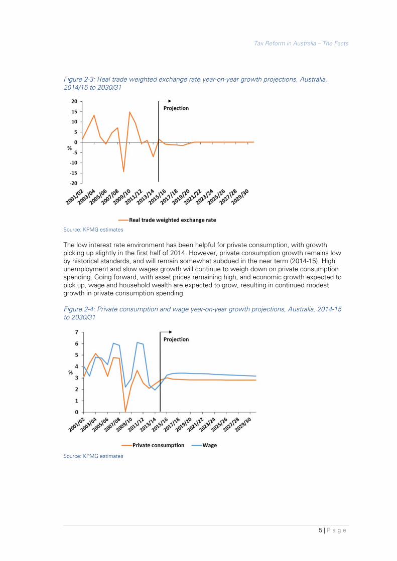
Figure 2-3: Real trade weighted exchange rate year-on-year growth projections, Australia, 2014/15 to 2030/31


The low interest rate environment has been helpful for private consumption, with growth picking up slightly in the first half of 2014. However, private consumption growth remains low by historical standards, and will remain somewhat subdued in the near term (2014-15). High unemployment and slow wages growth will continue to weigh down on private consumption spending. Going forward, with asset prices remaining high, and economic growth expected to pick up, wage and household wealth are expected to grow, resulting in continued modest growth in private consumption spending.

Figure 2-4: Private consumption and wage year-on-year growth projections, Australia, 2014-15 to 2030/31



6 | P a g e

With the import-intensive investment phase of the resources sector capacity expansion ending, imports are expected to grow at a slower pace in 2015/16. Going forward, imports growth is expected to be supported by household consumption.

At the same time, an increase in exports growth can be expected from 2016-17. Resource exports, particularly LNG exports, are expected to pick up pace from 2016.

Figure 2-5: Exports and imports year-on-year growth projections, Australia, 2014-15 to 2030/31


A recent OECD study shows that tax revenues in many OECD countries are now back above their pre-global financial crisis (GFC) levels. While personal and company income taxes are still the main contributors to government revenues across most of these countries, the OECD continues to warn against the distortive nature of these taxes.4

The new OECD research also finds that there is a general trend towards consumption taxes among its member countries. Many countries, particularly those in the European region, have increased their standard value-added taxes (VAT) over the last 5 years, with an increase of 1.5 per cent in the average standard VAT observed between January 2009 and 2014. While there is also a potentially significant boost to revenue associated with VAT base-broadening, this remains a less popular approach to increasing taxation revenues.5

The OECD and the Korea Institute of Public Finance recently undertook a joint study into the distributional effects of consumption taxes in 20 OECD countries. Consumption taxes are generally seen as regressive. The poor are believed to be most impacted by taxes on consumption, as a greater proportion of their incomes is spent on necessities such as food. While this is true when measured as a percentage of income, the study shows that the opposite is true in most cases when measured as a percentage of expenditure from a lifetime perspective.

4 OECD (2014), Revenue Statistics 2014, OECD Publishing. 5 OECD (2014), Consumption Tax Trends 2014: VAT/GST and excise rates, trends and policy issues, OECD Publishing.

(%)


7 | P a g e

The study also suggests that reduced VAT rates which are aimed to benefit the poor and promote social welfare may not always work as expected in practice. In some cases, the rich benefit more from reduced rates on items such as hotel accommodation and restaurant food.6

Like many other OECD countries, personal income tax, company tax and GST are the three major sources of tax revenue for Australian governments. The figure below shows the level of tax revenue raised by the Australian Government across these three taxes. Studies have shown that income taxes levied on individuals and on consumption are relatively efficient taxes, while those levied on highly mobile bases (such as capital – or company – taxes) are less efficient (see Appendix B).

In addition to their GST redistributions, state governments rely on payroll tax, stamp duties, and taxes on motor vehicles, land, gambling and insurance. Many of these state taxes have been shown to distort behaviour and are thus identified as relatively inefficient (see Appendix B).

Figure 2-6: Australian taxation revenue ($ million)

Source: Australian Bureau of Statistics, Taxation Revenue, Australia

According to the latest government budget, total federal government taxation revenue is estimated to be around 22.1 percent of GDP in 2014-15, an increase of 1.7 percentage points from the previous period. Despite this increase, total taxation revenue will still fall short of total federal government spending, which is estimated to reach 25.4 per cent of GDP. Based on Treasury’s budget projections, this fiscal gap will remain in the outer years of the budget despite expected small increases in total taxation revenue, with total government expenditure remaining relatively stable at around 25.3 per cent of GDP in 2017-18.

Demographic change, mainly driven by our ageing population, is expected to escalate future fiscal pressures. Slower economic growth resulting from a shrinking working-age population and higher costs of healthcare will continue to worsen the fiscal budget position in the long run. According to Treasury’s 2010 Intergenerational Report, ageing and health pressures will cause

6 OECD/Korea Institute of Public Finance (2014),The Distributional Effects of Consumption Taxes in OECD Countries, OECD Tax Policy Studies, No. 22, OECD Publishing.

2009-10 2010-11 2011-12 2012-13Personal income tax 124,941 138,532 153,760 162,993Company income tax 54,490 57,071 66,435 70,117GST 46,553 48,093 48,849 50,313Crude oil and LPG excise 15,766 16,305 16,924 17,839Other excises 8,781 9,497 8,557 7,871Income tax paid by superannuation funds 6,164 6,683 7,838 7,574Taxes on international trade 5,762 5,839 7,117 8,181Other federal taxes 5,221 7,100 8,068 13,476

Total federal government 267,678 289,120 317,548 338,364Payroll tax 16,761 17,955 19,747 20,752Stamp duties on conveyances 12,292 12,430 11,658 12,841Municipal rates 11,669 12,506 13,290 14,192Motor vehicle taxes (including stamp duty on registration) 6,992 7,461 7,884 8,532Land taxes 5,767 6,005 6,103 6,192Gambling taxes 5,054 5,147 5,370 5,493Insurance taxes 4,597 5,035 5,394 5,526Other state and local taxes 3,064 4,112 3,521 3,883

Total state and local government 66,196 70,651 72,967 77,411

Total 333,874 359,771 390,515 415,775


8 | P a g e

total government spending to reach 27.1 per cent of GDP by 2049-50, exceeding total government revenue by almost 3 per cent of GDP.

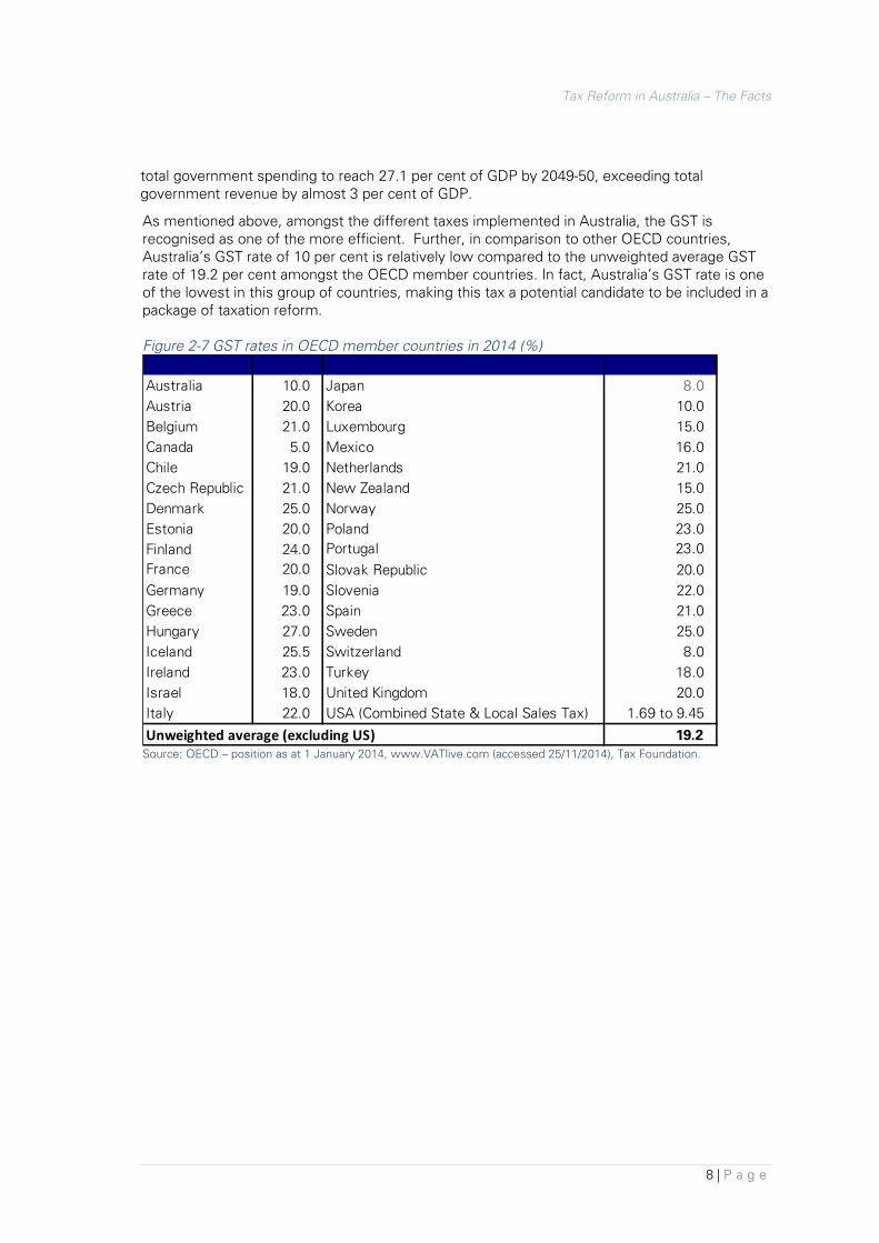
As mentioned above, amongst the different taxes implemented in Australia, the GST is recognised as one of the more efficient. Further, in comparison to other OECD countries, Australia’s GST rate of 10 per cent is relatively low compared to the unweighted average GST rate of 19.2 per cent amongst the OECD member countries. In fact, Australia’s GST rate is one of the lowest in this group of countries, making this tax a potential candidate to be included in a package of taxation reform. Figure 2-7 GST rates in OECD member countries in 2014 (%)

Source: OECD – position as at 1 January 2014, www.VATlive.com (accessed 25/11/2014), Tax Foundation.

Australia 10.0 Japan 8.0Austria 20.0 Korea 10.0Belgium 21.0 Luxembourg 15.0Canada 5.0 Mexico 16.0Chile 19.0 Netherlands 21.0Czech Republic 21.0 New Zealand 15.0Denmark 25.0 Norway 25.0Estonia 20.0 Poland 23.0Finland 24.0 Portugal 23.0France 20.0 Slovak Republic 20.0Germany 19.0 Slovenia 22.0Greece 23.0 Spain 21.0Hungary 27.0 Sweden 25.0Iceland 25.5 Switzerland 8.0Ireland 23.0 Turkey 18.0Israel 18.0 United Kingdom 20.0Italy 22.0 USA (Combined State & Local Sales Tax) 1.69 to 9.45

Unweighted average (excluding US) 19.2


9 | P a g e

OECD data on taxation compositions across different countries shows that Australia’s total taxation mix is skewed towards direct taxes (individuals and corporations). According to the OECD, these taxes contributed almost 60 per cent of total Australian tax revenue in 2013, compared to an OECD average of just over 30 per cent.

Figure 2-8 2013 tax revenue as a share of total taxation (%)

Source: OECD, OECD.StatExtracts, http://stats.oecd.org/#, accessed February 2015. Notes: 1. “Individuals” includes Taxes on income, profits and capital gains paid by individuals. 2. “Corporate” includes Taxes on income, profits and capital gains paid by corporate. 3. “Other taxes” include those not already identified, and also unallocated Taxes on income, profits and capital gains and unallocated Social security payments.

Individuals CorporateSocial

Security Contributions

Value Added Taxes

Other goods and

services

Payroll and workforce

PropertyOther taxes

Australia 39.2 18.9 12.1 16.0 5.2 8.6Canada 36.6 9.5 15.5 13.7 10.8 2.1 10.6 1.2New Zealand 37.7 14.1 30.0 8.3 6.2Greece 20.6 3.3 32.0 21.2 16.6 5.6 0.4Iceland 37.4 5.4 10.4 22.8 12.3 0.9 7.1 3.8United Kingdom 27.5 8.1 19.1 20.8 12.1 11.9Switzerland 31.7 10.5 24.9 13.0 9.9 6.6 3.4Turkey 14.4 7.4 27.2 20.8 24.2 4.2 1.7United States 37.7 10.2 22.3 17.9 11.8OECD - Average 24.5 8.5 26.2 19.5 13.3 1.1 5.5 1.5


10 | P a g e

Since the 2011 Tax Forum, little has been done in the area of tax reform. Going forward, the Australian Government has committed to undertake a comprehensive review on tax reform, in consultation with the public, within the next two years. They also plan to have proposals for further tax reform on the agenda in the next Federal election.

To further advance the debate on tax reform in Australia, CPA Australia has engaged KPMG to update and extend the 2011 KPMG GST analysis. The scenarios presented in this report are designed to be illustrative examples of the potential gains from some tax reform options. The following four alternative GST designs are examined.

1. 10% GST on a broader base – extending the GST coverage to include fresh food, health and education. In 2015-16, this is estimated to raise an additional $12.1 billion in GST revenue. This additional revenue is used to abolish insurance taxes, stamp duty on motor vehicles and a small proportion (9 per cent) of conveyancing stamp duty. Any remaining additional GST revenue is returned to households through personal income tax cuts and welfare payments.

2. 15% GST with current exemptions – increasing the statutory rate of GST to 15 per cent. In 2015-16, this is estimated to raise an additional $26.0 billion in GST revenue. This additional revenue is used to abolish insurance taxes, stamp duty on motor vehicles and 80 per cent of conveyancing stamp duty. Any remaining additional GST revenue is returned to households through personal income tax cuts and welfare payments.

3. 15% GST and applied to health and education – increasing the statutory rate of GST to 15 per cent and extending the GST coverage to include health and education. In 2015-16, this is estimated to raise an additional $36.8 billion in GST revenue. This additional revenue is used to abolish insurance taxes, stamp duty on motor vehicles and all conveyancing stamp duty. Any remaining additional GST revenue is returned to households through personal income tax cuts and welfare payments.

4. 15% GST on a broader base – increasing the statutory rate of GST to 15 per cent and extending the coverage to include fresh food, health and education. In 2015-16, this is estimated to raise an additional $42.9 billion in GST revenue. This additional revenue is used to abolish insurance taxes, stamp duty on motor vehicles and all conveyancing stamp duty. Any remaining additional GST revenue is returned to households through personal income tax cuts and welfare payments.

This report examines scenarios looking at variations in the application of the 10 per cent GST and a 15 per cent GST have been chosen. In contrast to the 2011 study, this analysis does not examine 12.5 per cent or 20 per cent GST scenarios. This is because the 2011 work showed that a 12.5 per cent GST is unlikely to provide much scope for reforming other taxes in the system, while a 20 per cent GST scenario is less tenable in the current political environment.

While these scenarios show that there are potential benefits associated with GST-led tax reform, it is acknowledged that the final design of tax reform must take into consideration many other factors. These would include, but not be limited to, assessment of other options around tax mix switches, welfare impacts across different socio-economic groups, fiscal implications at all levels of government (including the implications on horizontal and vertical equalisation), and implementation issues such as grandfathering and compliance costs.

It should be noted any change in compliance costs associated with changes to the application of the GST is beyond the scope of this analysis. While these costs are likely to be one-off and relatively small, they should still be examined and factored into any final policy design process.


11 | P a g e

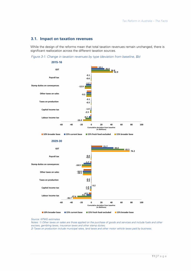
While the design of the reforms mean that total taxation revenues remain unchanged, there is significant reallocation across the different taxation sources.

Figure 3-1: Change in taxation revenues by type (deviation from baseline, $b)

2015-16

2029-30

Source: KPMG estimates Notes: 1) Other taxes on sales are those applied on the purchase of goods and services and include fuels and other excises, gambling taxes, insurance taxes and other stamp duties; 2) Taxes on production include municipal rates, land taxes and other motor vehicle taxes paid by business.

12.1

-0.1

-1.2

-0.1

26.0

-1.0

-4.7

36.8

-0.6

-12.9

-9.5

-0.5

42.9

-2.5

-16.4

-60 -40 -20 0 20 40 60 80 100

GST

Payroll tax

Stamp duties on conveyances

Other taxes on sales

Taxes on production

Capital income tax

Labour income tax

Cumulative deviation from baseline(in $billions)

10% broader base 15% current base 15% fresh food excluded 15% broader base

21.7

-1.7

0.2

-4.9

44.0

-0.4

-16.9

-0.3

-1.9

-9.5

65.5

-0.8

-18.9

-16.5

-0.2

-1.6

-27.6

76.2

-36.7

-60 -40 -20 0 20 40 60 80 100

GST

Payroll tax

Stamp duties on conveyances

Other taxes on sales

Taxes on production

Capital income tax

Labour income tax

Cumulative deviation from baseline(in $billions)

10% broader base 15% current base 15% fresh food excluded 15% broader base


12 | P a g e

The tax policies raise different amounts of GST – depending on the rate and application across the consumption base. In 2015-16, average annual additional revenue raised across the four scenarios is estimated at between $12 billion and $43 billion. By 2029-30, average annual additional revenue raised across the four scenarios is estimated at between $21 billion and $76 billion.

This revenue is used to retire a number of taxes including:

• Insurance taxes and stamp duties on motor vehicles are abolished in all four scenarios - these taxes are both included in the other taxes on sales column in the figure above, and are estimated at around $8.5 billion in revenues in 2015-16

• stamp duties on property conveyancing – in the first and second scenarios, the duty applied to conveyancing has been reduced by 9 per cent and 80 per cent, respectively. In the last two scenarios, all of this duty has been abolished. Tax revenue collected through property conveyancing duty was estimated at around $12.9 billion in 2015-16; and

• personal income tax – there is also extra revenue from GST beyond that which is spent on retiring the taxes discussed above. This revenue has been returned to households by way of personal tax cuts and welfare payments. Overall labour income taxes reduced by between $1.8 billion and $16.4 billion under these alternative policies (in 2015-16). While annual welfare payments equivalent to between $89 million and $939 million were provided under the scenarios’ compensation packages in that same year.

In each scenario, additional revenue is collected from the GST. This, by itself, would increase the average tax rate on the economy, increasing prices for goods and services and providing disincentives to supply of labour through the reduction in real take-home wages.

However, higher GST revenues also mean that a selection of other taxes can be abolished. This would reduce the cost of particular goods and services (insurance, motor vehicle costs and stamp duty on conveyances). In all scenarios, some of the additional tax revenue is also returned to households in the form of lower personal income tax collections. This leads to an overall increase in real incomes.

With the GST currently at a relatively low 10 per cent, the efficiency cost of increasing the rate by 5 per cent is smaller than the benefits of reducing or abolishing other taxes that are imposed on smaller bases at higher rates.

The benefits will take a few years to properly flow through to the economy, as wages take time to adjust. Taxes that impact capital will also take some time to flow through the economy, as capital stock purchased under the current tax policies is gradually replaced by new capital stock purchased under these new tax policies.

The impacts of these tax reforms are likely to vary considerably across different individuals. Specifically, those groups who were more exposed to the taxes abolished will tend to benefit the most from the tax reform, whilst those who have a larger exposure to the GST will tend to either benefit less or be negatively impacted upon. For example, the low income groups generally spend a higher proportion of their disposable incomes on consumption goods, and without additional redistribution, would receive less (if anything) back through a reduction in personal income tax rates.


13 | P a g e

To offset some of this inequality, the figure below shows how CPA Australia has chosen to redistribute the tax revenue through the personal income tax system. This redistribution is illustrative only, and could take many forms. The redistribution below was chosen so as to provide greater tax cuts to the lower income earners where possible.

Figure 3-2: Change in average personal income tax rates by income bracket (percentage deviation from baseline, 2015-16)


The change in personal income tax rates in the figure above largely reflects the assumed changes in income tax brackets that have been input into the analysis (see Appendix B for more details). Slight variations will also occur as the economy adjusts to the new tax policies through changes in both labour supply and average wages. This can be illustrated in the first scenario results above – as this scenario has very little changes to the tax brackets applied.

In addition to these tax cuts, low income households were provided with an additional annual support payment, discussed in more detail below.

The figure below shows how the tax policies (including these additional support payments) flow through to an overall impact on the wellbeing of different groups in the economy. The overall impact on real incomes takes into account the impact of the taxation policy on each group’s current expenditure bundle and composition of income.

The income groups in this analysis are based on the Australian Bureau of Statistics (ABS) equally sized household income quintiles7.

7 In the ABS household groups, households are ranked from the lowest on the basis of their household

income. The population is divided into five equally sized groups called quintiles, thus the first quintile will comprise the first 20 percentiles. Equivalised disposable household income is the income measure used to define the quintiles – the quintiles each comprise the same number of persons, that is, they are person weighted. In 2009-10, the average equivalised disposable income of households associated with the five household income quintiles was calculated at $30,628 (lowest quintile), $54,080 (second quintile), $77,844 (third quintile), $108,524 (fourth quintile) and $190,060 (highest quintile) - based on data from Australian Bureau of Statistics, 2014, “Catalogue no. 6523.0 Household Income and Income Distribution, Australia - Detailed tables, 2009-10”.

-0.2

-0.9

-1.9

-2.9

-0.2

-0.9

-1.8

-2.6

-0.1

-0.9

-1.8

-2.6

0.0-0.5

-1.2

-1.8

-4.0

-2.0

0.0

2.010% broader base 15% current base 15% fresh food excluded 15% broader base

%

$0 - $35,000 $35,001 - $80,000 $80,001 - $180,000 $180,001+


14 | P a g e

Figure 3-3: Change in real (after-tax) incomes by household income quintile 8 (percentage deviation from baseline, 2015-16)

Source: KPMG estimates Note: Household income includes all current receipts (monetary or in kind) received by the household and which are available for, or intended to support, current consumption. This income includes receipts from: wages and salaries and other receipts from employment; profit/loss from unincorporated business; net investment income (interest, rents, dividends, royalties), government pensions and allowances; and private transfers (e.g. superannuation, workers’ compensation, child support).

The broadening and/or increase in the GST tends to have a proportionally higher impact on household costs for the lower income quintiles than for the higher income quintiles.

Further, the lowest income quintile gains little from the redistribution of revenues purely through personal tax, as these households have little interaction with the tax system. To assist these households with the additional costs associated with GST adjustments, we have first redistributed some of the GST revenue through annual support payments. The remainder is then distributed across all taxpayers through the adjustments to the personal income tax system (brackets and rates – as shown in the previous figure).

The other quintiles benefit from both increased incomes as a result of improved efficiency in the economy and the redistribution of the GST revenue through the tax system. Most importantly, these groups are able to access significant personal tax reductions, which more than offset their increase in consumption costs.

8 The data indicates, and thus the analysis assumes, that lower income households tend to have one

income earner, while the higher income houses have two income earners, on average.

0.8

0.7

0.2

0.0

0.8

0.7

0.00.0

1.0

0.6

0.10.1

0.5

0.4

0.10.0

0.7

0.4

0.10.0

0.0

0.2

0.4

0.6

0.8

1.0

1.215% broader base15% fresh food excluded15% current base10% broader base

%

Lowest quintile Second quintile Third quintile Fourth quintile Highest quintile


15 | P a g e

Figure 3-4: Change in real (after-tax) incomes by household income quintile9 ($ deviation from baseline, 2015-16)


The redistribution applied in this analysis has been designed to give each household a similar percentage change in real (after-tax) income (as observed in the previous chart). When this is converted into dollar changes, it can be seen that some households benefit more than others under this illustrative redistribution. In all scenarios, all households receive a boost to their real incomes. As these illustrative results show, while using the tax and welfare system to redistribute the additional GST revenues has gone some way towards sharing the benefits of the reform, further analysis of the redistribution methods would be required.

9 This is calculated as the change in the cost of the households original expenditure bundle (before the household responds to the new price signals) compared to the change in their after tax incomes.

1785

239 273

29 28

398 461

64 127

509

898

36108

433564

20143

918

1,551

0

250

500

750

1,000

1,250

1,500

1,75010% broader base 15% current base 15% fresh food excluded 15% broader base

$

Lowest Second Third Fourth Highest


16 | P a g e

The use of GST to replace a set of relatively less efficient taxes also leads to different impacts across different industries.

Figure 3-5: Change in value-added by industry (percentage deviation from baseline, 2029-30)


The figure above shows that, while most sectors are expected to be larger because of the simulated tax reforms, there are some sectors that are expected to be smaller than would otherwise be the case.

In the first scenario, the rate of GST is unchanged, but the base is broadened to include items that are currently untaxed – fresh food items, health and education. As a result, while the price of most items will not be directly affected by the uniform GST, the price of items that are currently GST-free would be higher. This is reflected in the results above, with the education and health industries showing lower output under this scenario.

2.5

0.7

0.1

0.4

0.8

-1.6

0.5

-0.8

0.7

2.1

-2.0

0.0

-0.1

0.5

0.3

-0.3

-0.1

0.2

4.0

-1.0

1.1

0.9

1.5

-1.8

0.5

-0.9

1.1

4.4

-0.5

0.6

0.9

1.8

-1.6

0.6

-0.8

1.2

-3.0 -2.0 -1.0 0.0 1.0 2.0 3.0 4.0 5.0

Financial and Insurance Services

Accommodation and Food Services

Retail Trade

Manufacturing

Construction

Health Care and Social assistance

Transport, Postal and Warehousing

Education and Training

Other industries

Cumulative deviation from baseline (in percentage

points)

Sc1 - 2029-30 Sc2 - 2029-30 Sc3 - 2029-30 Sc4 - 2029-30


17 | P a g e

In the other three scenarios, the rate of GST is raised. By itself, this will tend to raise the overall price level, and reduce overall demand, along with economic activity. However, in all scenarios, any additional GST revenue is used to reduce or completely abolish a number of other taxes in the economy.

An important influence on the level of activity in the finance and insurance sector is that of taxes on insurance. In all scenarios, insurance taxes are abolished. This lowers the price of insurance products, leading to higher demand for insurance products. This contributes to the higher level of activity in the finance and insurance sector, as can be seen in the figure above.

Another common factor across all four scenarios is the abolition of stamp duty on motor vehicles. This reform reduces the cost of purchasing motor vehicles. Overall the abolition of motor vehicle taxes will directly benefit industries and households, and also indirectly benefit by reducing the costs of production in the economy.

Conveyancing stamp duty has also been fully (or close to) abolished in the last three scenarios. This reduces property costs, which encourages greater activity in the property sector. As a result, construction services and property and business services are both in higher demand, which is reflected in the figure above.

In all scenarios, once the impacts have had time to flow through the economy, GDP is higher than would otherwise be the case.

While the higher GST will have a higher negative impact on output, there will be positive GDP impacts from the abolition of less efficient taxes. The gains in economic activity are largely attributed to the removal of inefficient state taxes. The final three scenarios all involve increasing the GST to 15%, which should raise enough revenue to abolish all insurance, motor vehicle stamp duty and all (or most of) conveyancing duty. In the years where the additional GST is more than enough to retire/reduce the chosen taxes, this additional revenue is then redistributed via the personal income tax system and welfare payments.

Figure 3-6: Change in GDP (deviation from baseline, % change and current dollars)


0.6 ($16.1b)

0.1 ($3.1b)

0.9 ($23.6b)

1.0 ($27.5b)

-0.6

-0.4

-0.2

0.0

0.2

0.4

0.6

0.8

1.0

1.2

Cum

ulat

ive

devi

atio

n fro

m b

asel

ine

(in p

erce

ntag

e po

ints

)

10% broader base 15% current base15% fresh food excluded 15% broader base


18 | P a g e

Figure 3-7: Change in GDP by components (percentage deviation from baseline)


The change in GST will impact consumption in the economy through an increase in prices. The change in the other taxes will stimulate activity and boost consumption and investment.

The tax reforms will also positively affect Australia’s interactions with the rest of the world by affecting the cost of producing exports and the exchange rate.

The imposition of GST does not increase the price of exports because all exports are GST-free. On the other hand, the reduction of other taxes reduces the cost of production in Australian industries. These reforms also improve the productivity of Australian industries by removing distortions to the way that resources are allocated across the economy. Overall, the modelling indicates that the price of Australian exports on the foreign market is lower than would otherwise be the case, making Australian producers more competitive in the international market. This raises the demand for exports, which puts upward pressure on the exchange rate.

A stronger Australian dollar makes imports relatively cheaper than under the baseline, leading to higher demand for imports also. The model assumes that the balance of trade is fixed in the long-term (a standard long-run model assumption), and further adjustments to the exchange rate will occur until the trade balance returns to its original level.

0.6

0.9

1.3

0.9

0.30.5

0.0

0.6

1.2

1.6

0.9

1.31.5

1.8

0.8

1.5

-1

0

1

1

2

2

H'hold consumption Investment Exports Imports

Cum

ulat

ive

devi

atio

n fr

om b

asel

ine

(in p

erce

ntag

e po

ints

)

10% broader base - 2029-30 15% current base - 2029-3015% fresh food excluded - 2029-30 15% broader base - 2029-30


19 | P a g e

This attachment discusses and presents the economic modelling approach used to estimate the economic impact of alternative tax policies. To estimate these economic impacts, this study employed a dynamic, computable general equilibrium (CGE) model, described further below.

To model the economic impact of a change in tax policy – capturing the flow-on impacts beyond those that directly relate to the economic agent on whom the legal incidence of the tax falls (e.g. industry, consumer and employee) – it is necessary to employ a modelling technique that makes use of information about linkages across the broader economy. Input-output (IO) tables published by the ABS provide detailed information on the upstream and downstream linkages in the economy.

• The upstream linkages of an industry refer to the sources of inputs that go into the production of goods and services. These linkages may be in the form of the use of intermediate inputs produced by other domestic industries, imported intermediate inputs, labour and other factors of production. For example, manufacturing would use inputs such as labour, electricity, unprocessed minerals or foods, fuel, and services such as those provided by the transport industry. This can be thought of as information regarding the cost-side of the economy.

• Downstream linkages of an industry refer to those economic agents that purchase the goods and services (e.g. the manufacturing sector’s output). For example, the restaurants sector might purchase manufactured food as part of its operations or the business services sector might purchase paper products and computers. Consequently, downstream linkages include sales to other industries that use the goods and services as an intermediate input to their own production process or final users of the product like households, the government or foreigners. This can be thought of as information regarding the sales-side of the economy.

An IO table is a useful tool as a snapshot of the economic flows within the economy at the time the data was collected. An input-output table can be used to provide simplified estimates of the sensitivity of the economy (measured by employment, value added or turnover) to small changes (termed ‘shocks’) within industries. An example of such a shock might be a ten per cent increase in the fuel excise. This would lead to a cost increase for all industries that use fuel, particularly impacting those industries whose inputs comprise a relatively large proportion of fuel. This sort of analysis can be used at the industry-wide level to estimate IO multipliers – that is, the total economy-wide impact on employment or output resulting from a change in one industry, taking into account the change in demand for the outputs of other industries.

An IO table in itself is not an economic model, and IO multipliers are raw and ad hoc in nature. A major limitation of the use of IO multipliers when used to conduct impact analysis is that the relationship between industry inputs and outputs (the coefficients) are fixed, implying that industry structure remains unchanged by the shock to the industry (for example, a change in demand or prices). Furthermore, IO analysis imposes no resource constraints and so industries (and indeed the entire economy) can access unlimited supplies of inputs at fixed costs.

In reality, scarcity of inputs (e.g. skilled labour, land etc.) mean that these inputs are affected by and respond to changes in prices (e.g. wages) driven by supply and demand adjustments. For example, if one industry demands more labour, this will (generally) drive up average wages and will, at the margin, increase costs in other sectors and reduce demand for labour by some other parts of the economy.


20 | P a g e

In IO analysis, where all adjustments relate only to quantities produced, this type of feedback response does not to occur, and sectors can access infinite amounts of inputs at fixed costs. Consequently, an IO model can result in an overstatement of the impacts on the economy. For these reasons, while the ABS did for some time publish IO multipliers, it has ceased publishing these estimates in recent years over concerns about their validity.

A computable general equilibrium (CGE) model makes use of an IO table in the construction of its database, but is extended to make more sophisticated economic and behavioural assumptions including:

• recognising resource constraints and responses of businesses, workers through adjusting prices/wages;

• capturing employment/capital (and other factors inputs) substitution for example, by responding to higher wages by increasing the use of capital;

• capturing a much wider set of economic impacts such as behavioural responses to price changes of consumers, investors, foreigners etc.; and

• can include the effects of such things as technological change and shifts in consumer preferences.

By introducing these additional economic variables and constraints, CGE models are able to model beyond the first round impact of an event or policy, account for scarcity and understand behavioural response to economic variables. This added sophistication means that a CGE model allows for feedback responses by producers, consumers, investors and foreigners and so the results are less likely to be overstated particularly over the medium to long run.

The KPMG FLAGSHIP model has been developed by Dr Ashley Winston, KPMG Australia’s Chief Economist, with assistance from the KPMG economic modelling team. FLAGSHIP brings together 80 years of combined modelling experience (gained with the world’s pre-eminent economic modelling institutions, and in economic policy advice and research roles with several international governments), the latest theoretical developments in the field and a database constructed from the latest available data.

FLAGSHIP is a development of the world-leading ORANI and MONASH model lineage created at the Centre of Policy Studies, and is based in the powerful GEMPACK modelling software. FLAGSHIP brings the best of this world-renowned modelling tradition together with several new theoretical advancements – developed by Dr Winston as part of economic modelling and policy work with the US government – to create a cutting-edge CGE framework.

The model embodies an array of features that enhance its utility in policy and economic modelling.

• Simulation design can be carried out with enormous flexibility, limited only by the economist’s imagination and the constraints of economic theory. Experimental design is a key element of robust economic modelling. For example, the FLAGSHIP model can be run in both comparative static or dynamic modes, and is not limited by traditional “short-run” and “long-run” structural constraints.

• The core model distinguishes 114 sectors and 114 commodities, based on the latest ABS input-output tables (2009/10), with the ability to expand this dimensionality at will.

• Primary factor inputs distinguish multiple types of capital, labour, land, natural resource endowments.


21 | P a g e

• On the input side, the multi-level production nest (in CRESH functional form) allows almost limitless flexibility in the setting of substitution and technology parameters, including the ability to change functional form with ease. Energy goods are treated separately to other intermediate goods and services in production, and are complementary to capital.

• On the output side, FLAGSHIP applies a structure (nested CRETH transformation) that accommodates multi-product industry sectors and their choice of final output bundles. This structure also allows a great deal of flexibility in setting substitution possibilities and technology, and allows the functional form of the nest to be modified with ease. The model also distinguishes between a given commodity or service that is produced by several industries (heterogeneous), and distinguishes between goods and services destined for export markets and those destined for domestic sales.

• The core model distinguishes 9 labour occupations partitioned into low-skilled and high-skilled groups, with the capacity to expand this detail to several hundred occupations. The supply of labour is determined by a labour-leisure trade-off that allows workers to respond to changes in after tax wages and the price of net national income in determining the hours of work they offer to the labour market. Leisure enters the worker’s utility function.

• Household consumption decisions distinguish between subsistence (necessity) and discretionary (luxury) consumption. The nature of the consumption bundle that can be financed by household disposable income influences decisions between leisure and work.

• International trade is disaggregated by source and destination for imports and exports respectively, with the ability to distinguish over 100 foreign regions (dependent on application).

• FLAGSHIP contains emissions accounts, explicit modelling of both combustion and fugitive greenhouse emissions, and the ability to analyse an array of carbon policy regimes (including cap-and-trade, a carbon tax and direct regulation). Multiple electricity technologies are explicitly modelled. FLAGSHIP embodies other energy technologies

• Detailed government fiscal accounts and balance sheet are modelled, including the accumulation of public assets and liabilities, based on GFS statistics. Detailed government revenue flows are modelled, including over 20 direct and indirect taxes and income from government enterprise, and government spending includes public sector consumption, investment and the payment of various types of transfers (such as pensions and unemployment benefits).

• Investment behaviour is closely linked with detailed modelling of business taxation and a variety of capital allowances, including the structure of the imputation system (which can be switched on and off), and representative firms in each sector are able to choose between debt, equity and retained earnings in determining their cost of capital. The available supply of financial sources includes an assessment of the availability of retained earnings (both franked and unfranked), the cost of debt tied to a leverage function, and both debt and equity face underwriting and transaction costs that vary with size of the flow.

• Foreign asset and liability accumulation is explicitly modelled, as are the cross-border income flows they generate and which contribute to the evolution of the current account. Along with other foreign income flows like labour payments and unrequited transfers, FLAGSHIP takes account of primary and secondary income flows in Australia’s current account; these are particularly important in the Australian context as they typically comprise the bulk of the balance on the current account.

• The modelling suite includes a database construction routine that allows rapid adjustments to be made to the FLAGSHIP database, most importantly in the modification of the database as new information is released. This ensures that the FLAGSHIP database is always as up-to-date as data availability allows, and can be adjusted at will according to the needs of simulation design and model development.


22 | P a g e

B.1 The economic cost of alternative forms of taxation

Taxes are used to fund important government services, such as education, health and welfare. However, taxes also affect the way that the economy operates, and can lead to less productive use of the resources available in Australian economy, and lower living standards.

Most taxes distort economic activity to some extent. This is because most taxes change the behaviours of participants in the economy. When taxes affect the choices made by households, businesses and the foreign sector, the economy does not operate in its most productive way. For example, if taxes reduce the incentive to work, then employment would be lower than would otherwise be the case, leading to lower household incomes. If taxes affect firms’ operating decisions, and result in resources not being allocated to their most efficient uses, then the productivity of these resources will be lower. These productivity impacts, in turn, impact on output and national income. In this way, taxes can result in a loss in living standards/ consumer welfare,10 over and above the revenue raised from the tax.

The extent to which a tax reduces living standards can be measured by its excess burden, which is the loss in living standards from a tax divided by the amount of revenue raised. The greater the excess burden of a tax, the greater the loss in living standards per dollar of revenue, and the less efficient the tax is said to be.

The excess burden of a tax is likely to be higher, the narrower or more mobile the tax base is. This is because it may be possible to respond to the tax by shifting to an untaxed substitute. If the tax is applied to a very narrow or a very mobile base, it is likely that there will be more options for substitution away from that base. Such shifts add to economic inefficiency and reduce the revenue yield.

The higher the tax rate, the higher will be the reduction in welfare. Moreover, if the tax rate increases, the excess burden increases at a greater rate.

GST is a broad-based tax on consumption, which is payable on most goods and services consumed in Australia. The GST is currently set at a relatively low 10 per cent rate. The main economic cost of GST is to raise the price level. This leads to a fall in the real wage or the real purchasing power of labour income, which may create a disincentive to work. This then flows through to reductions in consumption which, in turn, reduce the size of the overall tax base.

Since most goods and services are taxed, and taxed at the same rate, there is limited opportunity for households to avoid the GST by changing their consumption patterns.11 As a result, the GST does not have a large impact on the pattern of consumption, and thus has a relatively small impact on economic activity. Thus, the GST has a low excess burden.

Taxes on insurance are taxes on a narrow range of products. There are differences in application across the States and Territories, as an example – Term/Temporary and General Insurance duties range from between 5% and 11% of the premium paid depending on the 10 ‘Consumer living standards’ or ‘consumer welfare’ is the benefit derived by Australian households from consumption, savings and leisure time. It is a measure of aggregate welfare of all consumers in the economy. 11 However, there are some goods on which GST is not paid, such as fresh food. This does create some economic cost because households will substitute towards consuming these items to a certain extent, distorting the pattern of economic activity. Despite this inefficiency, the GST has a low overall excess burden because of its broad and immobile tax base.


23 | P a g e

state in question. Since household demand for insurance is relatively responsive to price, there is a relatively large distortion to economic activity per dollar of revenue raised by these taxes, leading to a high excess burden. On the other hand, types of insurance taken out by businesses are likely to be less responsive to price changes, and this offsets some of the excess burden.

Conveyancing stamp duties are levied on the value of property transactions, which includes the improved value (or capital value) of property. This means that they are a tax on both land and capital. When considered a tax on the transaction, these taxes are a significant proportion of the property transaction cost. They are considered to have a high excess burden, whether they are levied on commercial or residential properties.

Motor vehicle taxes also have a relatively high economic cost per dollar of revenue raised. Stamp duties are taxes on motor vehicle users (a tax on the transfer of vehicles), which means that they are taxes on families and business capital, and they increase the cost of investing in motor vehicles. In the case of business, registration fees lead to higher production costs. These taxes lead to a reduction in investment in motor vehicles, and a high excess burden.

Like GST, personal income tax (PIT) applies to labour income amongst other things. Although this tax reduces the incentive to work, labour supply has only a moderate responsiveness to changes in the after tax wage. However, PIT is a progressive tax, providing an exemption from tax on income earned up to the tax-free threshold, and imposing increasing marginal tax rates at higher incomes. Compared with a flat rate PIT, this progressivity may increase the disincentive to supply labour for individuals with higher income. This leads to a modest excess burden for PIT.

As discussed above, some taxes have higher costs per dollar of revenue than others. This implies that the negative impact of the tax system on the economy could be reduced by replacing some of Australia’s high-cost taxes with lower-cost taxes. In particular, many State taxes have relatively high economic costs, and reform to these taxes could result in economic gains. Consideration of the potential gains from such reforms is the focus of the tax policy designs examined in the body of this report.

B.2 Tax scenarios

This report investigates four scenarios in which the GST is used to pay for the abolition of a number of other (generally relatively inefficient state) taxes.

Each scenario looks at the level of reform that could be undertaken under alternative GST designs (rates or coverage). In each scenario, additional revenue is raised from the GST and the selected taxes are successively repealed, until overall government revenue is left unchanged. In doing so, a set of reforms with similar intent but of different scales are examined.

The scenarios presented in this report are designed to be illustrative examples of the potential gains from some tax reform options. The following four alternative GST designs are examined:

1. 10% GST on a broader base (to include fresh food, health and education) 2. 15% GST with current exemptions 3. 15% GST and applied to health and education 4. 15% GST on a broader base (to include fresh food, health and education).

Each scenario starts by abolishing relatively less efficient state taxes, in the following order, until revenue neutrality is reached:

1. Insurance Taxes – Insurance Duty 2. Motor Vehicle Taxes – Stamp Duty, and 3. Conveyancing Duty.


24 | P a g e

These taxes have been chosen because they have high economic costs per dollar of revenue (as discussed in the previous section). The first taxes to be abolished under each scenario are those with the smaller revenue yields, and have the potential to be relatively simple to reform. The last tax to be abolished is conveyancing duty – which is a tax with large revenue yield, thus requiring a much higher level of alternative funding.

In all scenarios, where the GST revenue is more than enough to compensate for the loss in revenue from abolishing selected taxes, the remaining GST revenue could be used to address other tax reform issues (including any equity concerns that may arise from changes to the tax system).

Those in the lowest income bracket may have little interaction with the personal income tax system. To assist these households with the additional costs associated with GST adjustments, we have first redistributed some of the GST revenue through annual support payments. The remainder is then distributed across all taxpayers through the adjustments to the personal income tax system.

The changes to the personal tax rates/brackets have been developed to allow the appropriate amount of personal income tax to be returned so that the additional GST raised under each policy is returned in full so that the overall tax take in each year remains the same as in the baseline.

The share returned across the income brackets has been designed so as to reduce the average income tax rate by more for the lower income brackets, as these groups are likely to be more impacted by the increase in costs associated with the higher GST. Any changes to the tax brackets and rates designed to assist those on lower incomes also flow through to benefit those in the higher income brackets.

It should be noted that issues surrounding redistribution are beyond the scope of this analysis and should be examined carefully when fully assessing any tax reform policy. For illustrative purposes, in CPA Australia’s scenarios in this report, any remaining revenue has been used to adjust personal tax rates / tax brackets as shown below.

These adjustments were designed so as to share the benefits and costs of the policy reforms across households in a relatively even way.

Figure B-1: Approximate change in personal tax schedules 2015-2016

current (2015/16)

10% broader

base

15% current

base

15% fresh food

excluded

15% broader

baseTax free bracket (Tax bracket 1) 18,200 18,200 18,500 19,500 20,000Tax rate - on income between tax bracket 1 and 2 19.0% 18.5% 17.0% 16.0% 13.5%Tax bracket 2 37,000 37,000 37,000 37,000 37,000Tax rate - on income between tax bracket 2 and 3 32.5% 32.5% 32.0% 31.5% 32.0%Tax bracket 3 80,000 80,000 80,000 80,000 80,000Tax rate - on income between tax bracket 2 and 3 37.0% 37.0% 36.1% 34.6% 33.1%Tax bracket 4 180,000 180,000 180,000 180,000 180,000Tax rate - on income above tax bracket 4 47.0% 47.0% 47.0% 47.0% 47.0%


25 | P a g e

C.1 Scenario 1: 10% broader base

Taxation revenues and key macroeconomic variables (deviation from baseline, $ million / per cent)

Change in real (after-tax) incomes by household income quintile in 2015-16 (deviation from baseline, $ per annum)

Description 2015-16 2016-17 2017-18 2018-19 2019-20 2020-21 2021-22 2022-23GST 12,120 12,780 13,351 13,924 14,499 15,112 15,770 16,462Insurance Duty -6,016 -6,301 -6,570 -6,862 -7,125 -7,409 -7,730 -8,083Motor Vehicle Stamp Duty -2,441 -2,589 -2,742 -2,935 -3,046 -3,157 -3,313 -3,521Conveyancing Duty -1,164 -1,196 -1,221 -1,263 -1,266 -1,281 -1,319 -1,381Other sales tax -211 -170 -165 -155 -136 -115 -93 -69Payroll Tax -150 -133 -130 -129 -126 -123 -121 -119Taxes on production -100 -78 -70 -62 -51 -40 -28 -16Capital Income Taxes -271 -369 -380 -366 -336 -304 -273 -240Personal Income Taxes (reduced taxes or increased welfare) -1,767 -1,944 -2,073 -2,151 -2,412 -2,682 -2,892 -3,033

0 0 0 0 0 0 0 0

Household consumption (% change compared to baseline) -0.41 -0.24 -0.18 -0.13 -0.07 -0.01 0.05 0.12Investment (% change compared to baseline) 0.47 0.48 0.54 0.59 0.65 0.70 0.73 0.75Exports (% change compared to baseline) 0.36 0.44 0.51 0.59 0.66 0.73 0.79 0.85Imports (% change compared to baseline) 0.30 0.36 0.42 0.46 0.52 0.56 0.60 0.64

Real GDP (% change compared to baseline) -0.11 -0.01 0.04 0.09 0.14 0.19 0.24 0.28

Description 2023-24 2024-25 2025-26 2026-27 2027-28 2028-29 2029-30GST 17,174 17,894 18,625 19,367 20,129 20,914 21,729Insurance Duty -8,445 -8,801 -9,150 -9,497 -9,847 -10,205 -10,573Motor Vehicle Stamp Duty -3,747 -3,967 -4,173 -4,368 -4,558 -4,748 -4,942Conveyancing Duty -1,444 -1,499 -1,545 -1,584 -1,621 -1,659 -1,699Other sales tax -43 -11 26 67 112 161 212Payroll Tax -117 -114 -110 -103 -95 -85 -72Taxes on production -3 11 26 43 61 81 101Capital Income Taxes -201 -151 -94 -31 34 102 169Personal Income Taxes (reduced taxes or increased welfare) -3,175 -3,362 -3,605 -3,893 -4,216 -4,561 -4,925

0 0 0 0 0 0 0

Household consumption (% change compared to baseline) 0.18 0.24 0.31 0.37 0.44 0.51 0.58Investment (% change compared to baseline) 0.76 0.77 0.79 0.82 0.84 0.86 0.88Exports (% change compared to baseline) 0.91 0.97 1.03 1.10 1.17 1.24 1.30Imports (% change compared to baseline) 0.67 0.70 0.73 0.76 0.79 0.83 0.86

Real GDP (% change compared to baseline) 0.32 0.37 0.41 0.46 0.51 0.56 0.60

Household quintile Lowest Second Third Fourth HighestINCREASE IN INCOME BEFORE TAX 97 79 21 24 5REDUCTION IN TAX / INCREASE IN INCOME SUPPORT 53 77 178 169 162TOTAL INCREASE IN INCOME (AFTER TAX) 150 156 199 193 167less: INCREASE IN COST OF EXPENDITURE 133 127 135 156 147REAL AFTER TAX INCOME 17 29 64 36 20


26 | P a g e

C.2 Scenario 2: 15% current base



Description 2015-16 2016-17 2017-18 2018-19 2019-20 2020-21 2021-22 2022-23GST 25,952 27,258 28,367 29,580 30,569 31,655 32,923 34,349Insurance Duty -6,016 -6,301 -6,570 -6,862 -7,125 -7,409 -7,730 -8,083Motor Vehicle Stamp Duty -2,441 -2,589 -2,742 -2,935 -3,046 -3,157 -3,313 -3,521Conveyancing Duty -10,348 -10,630 -10,852 -11,231 -11,251 -11,389 -11,729 -12,272Other sales tax -889 -856 -901 -950 -989 -1,022 -1,058 -1,096Payroll Tax -284 -278 -293 -306 -314 -321 -329 -339Taxes on production -293 -280 -279 -279 -274 -270 -269 -270Capital Income Taxes -972 -1,199 -1,257 -1,314 -1,337 -1,366 -1,407 -1,464Personal Income Taxes (reduced taxes or increased welfare) -4,709 -5,126 -5,474 -5,703 -6,233 -6,721 -7,089 -7,304

0 0 0 0 0 0 0 0

Household consumption (% change compared to baseline) -0.40 -0.20 -0.16 -0.12 -0.07 -0.03 0.01 0.05Investment (% change compared to baseline) 0.36 0.34 0.41 0.45 0.51 0.57 0.61 0.62Exports (% change compared to baseline) -0.15 -0.10 -0.07 -0.05 -0.01 0.04 0.07 0.09Imports (% change compared to baseline) -0.07 0.00 0.06 0.12 0.18 0.23 0.28 0.33

Real GDP (% change compared to baseline) -0.16 -0.05 -0.02 0.00 0.03 0.07 0.09 0.10

Description 2023-24 2024-25 2025-26 2026-27 2027-28 2028-29 2029-30GST 35,800 37,202 38,556 39,881 41,218 42,583 43,998Insurance Duty -8,445 -8,801 -9,150 -9,497 -9,847 -10,205 -10,573Motor Vehicle Stamp Duty -3,747 -3,967 -4,173 -4,368 -4,558 -4,748 -4,942Conveyancing Duty -12,834 -13,328 -13,733 -14,084 -14,412 -14,746 -15,098Other sales tax -1,136 -1,176 -1,216 -1,256 -1,297 -1,339 -1,382Payroll Tax -349 -357 -365 -371 -376 -382 -388Taxes on production -271 -271 -269 -268 -266 -265 -265Capital Income Taxes -1,524 -1,581 -1,635 -1,687 -1,739 -1,795 -1,854Personal Income Taxes (reduced taxes or increased welfare) -7,495 -7,721 -8,014 -8,351 -8,722 -9,103 -9,496

0 0 0 0 0 0 0

Household consumption (% change compared to baseline) 0.09 0.14 0.18 0.22 0.25 0.28 0.31Investment (% change compared to baseline) 0.61 0.59 0.57 0.54 0.52 0.49 0.47Exports (% change compared to baseline) 0.09 0.09 0.07 0.06 0.03 0.01 -0.03Imports (% change compared to baseline) 0.38 0.42 0.45 0.49 0.51 0.54 0.56


Household quintile Lowest Second Third Fourth HighestINCREASE IN INCOME BEFORE TAX 386 481 491 679 1,095REDUCTION IN TAX / INCREASE IN INCOME SUPPORT 214 331 721 796 1,210TOTAL INCREASE IN INCOME (AFTER TAX) 600 812 1,212 1,475 2,305less: INCREASE IN COST OF EXPENDITURE 514 785 1,085 1,367 2,162REAL AFTER TAX INCOME 85 28 127 108 143


27 | P a g e

C.3 Scenario 3: 15% fresh food excluded



Description 2015-16 2016-17 2017-18 2018-19 2019-20 2020-21 2021-22 2022-23GST 36,841 38,759 40,449 42,268 43,885 45,641 47,624 49,804Insurance Duty -6,016 -6,301 -6,570 -6,862 -7,125 -7,409 -7,730 -8,083Motor Vehicle Stamp Duty -2,441 -2,589 -2,742 -2,935 -3,046 -3,157 -3,313 -3,521Conveyancing Duty -12,935 -13,287 -13,565 -14,039 -14,064 -14,237 -14,661 -15,339Other sales tax -1,041 -993 -1,027 -1,059 -1,077 -1,081 -1,084 -1,083Payroll Tax -634 -634 -658 -681 -695 -709 -728 -750Taxes on production -473 -450 -439 -428 -409 -391 -375 -360Capital Income Taxes -1,760 -1,992 -2,007 -2,029 -1,984 -1,946 -1,925 -1,921Personal Income Taxes (reduced taxes or increased welfare) -11,542 -12,514 -13,441 -14,235 -15,484 -16,711 -17,809 -18,746

0 0 0 0 0 0 0 0

Household consumption (% change compared to baseline) -0.92 -0.62 -0.50 -0.36 -0.23 -0.09 0.05 0.20Investment (% change compared to baseline) 0.73 0.80 0.96 1.06 1.21 1.34 1.42 1.45Exports (% change compared to baseline) -0.12 -0.02 0.07 0.14 0.24 0.35 0.45 0.52Imports (% change compared to baseline) -0.03 0.10 0.21 0.33 0.45 0.56 0.66 0.75

Real GDP (% change compared to baseline) -0.37 -0.19 -0.09 -0.01 0.10 0.21 0.31 0.39

Description 2023-24 2024-25 2025-26 2026-27 2027-28 2028-29 2029-30GST 52,042 54,253 56,443 58,629 60,856 63,144 65,516Insurance Duty -8,445 -8,801 -9,150 -9,497 -9,847 -10,205 -10,573Motor Vehicle Stamp Duty -3,747 -3,967 -4,173 -4,368 -4,558 -4,748 -4,942Conveyancing Duty -16,043 -16,660 -17,167 -17,604 -18,015 -18,433 -18,873Other sales tax -1,079 -1,069 -1,056 -1,038 -1,018 -995 -969Payroll Tax -773 -792 -808 -819 -827 -830 -831Taxes on production -344 -324 -301 -276 -249 -221 -191Capital Income Taxes -1,908 -1,876 -1,826 -1,765 -1,702 -1,640 -1,583Personal Income Taxes (reduced taxes or increased welfare) -19,703 -20,764 -21,961 -23,260 -24,641 -26,073 -27,554

0 0 0 0 0 0 0



Household quintile Lowest Second Third Fourth HighestINCREASE IN INCOME BEFORE TAX 757 888 822 1,101 1,801REDUCTION IN TAX / INCREASE IN INCOME SUPPORT 263 639 1,370 1,559 2,699TOTAL INCREASE IN INCOME (AFTER TAX) 1,020 1,527 2,192 2,660 4,500less: INCREASE IN COST OF EXPENDITURE 780 1,129 1,683 2,227 3,582REAL AFTER TAX INCOME 239 398 509 433 918


28 | P a g e

C.4 Scenario 4: 15% broader base



C.5 Welfare payments

Total change in welfare payments in 2015-16 (deviation from baseline, $ per annum)

Description 2015-16 2016-17 2017-18 2018-19 2019-20 2020-21 2021-22 2022-23GST 42,892 45,102 47,053 49,152 51,041 53,085 55,382 57,896Insurance Duty -6,016 -6,301 -6,570 -6,862 -7,125 -7,409 -7,730 -8,083Motor Vehicle Stamp Duty -2,441 -2,589 -2,742 -2,935 -3,046 -3,157 -3,313 -3,521Conveyancing Duty -12,935 -13,287 -13,565 -14,039 -14,064 -14,237 -14,661 -15,339Other sales tax -1,283 -1,241 -1,285 -1,326 -1,348 -1,354 -1,360 -1,363Payroll Tax -798 -802 -832 -860 -875 -891 -913 -939Taxes on production -558 -536 -528 -518 -498 -479 -462 -447Capital Income Taxes -2,460 -2,740 -2,766 -2,811 -2,772 -2,741 -2,736 -2,754Personal Income Taxes (reduced taxes or increased welfare) -16,402 -17,607 -18,765 -19,802 -21,314 -22,817 -24,208 -25,450

0 0 0 0 0 0 0 0

Household consumption (% change compared to baseline) -1.01 -0.68 -0.55 -0.40 -0.24 -0.08 0.08 0.25Investment (% change compared to baseline) 0.81 0.91 1.11 1.23 1.41 1.56 1.65 1.70Exports (% change compared to baseline) -0.12 -0.03 0.05 0.11 0.21 0.33 0.43 0.50Imports (% change compared to baseline) -0.03 0.11 0.24 0.37 0.50 0.62 0.73 0.84

Real GDP (% change compared to baseline) -0.41 -0.21 -0.10 -0.01 0.12 0.24 0.35 0.44

Description 2023-24 2024-25 2025-26 2026-27 2027-28 2028-29 2029-30GST 60,480 63,039 65,581 68,123 70,719 73,387 76,158Insurance Duty -8,445 -8,801 -9,150 -9,497 -9,847 -10,205 -10,573Motor Vehicle Stamp Duty -3,747 -3,967 -4,173 -4,368 -4,558 -4,748 -4,942Conveyancing Duty -16,043 -16,660 -17,167 -17,604 -18,015 -18,433 -18,873Other sales tax -1,361 -1,352 -1,337 -1,316 -1,290 -1,260 -1,226Payroll Tax -966 -987 -1,004 -1,013 -1,019 -1,019 -1,016Taxes on production -429 -408 -382 -354 -324 -292 -258Capital Income Taxes -2,764 -2,752 -2,719 -2,672 -2,621 -2,572 -2,527Personal Income Taxes (reduced taxes or increased welfare) -26,725 -28,112 -29,649 -31,298 -33,045 -34,860 -36,744

0 0 0 0 0 0 0



Household quintile Lowest Second Third Fourth HighestINCREASE IN INCOME BEFORE TAX 1,006 1,210 1,166 1,573 2,585REDUCTION IN TAX / INCREASE IN INCOME SUPPORT 557 1,062 2,255 2,248 3,881TOTAL INCREASE IN INCOME (AFTER TAX) 1,563 2,273 3,422 3,821 6,465less: INCREASE IN COST OF EXPENDITURE 1,289 1,811 2,524 3,257 4,914REAL AFTER TAX INCOME 273 461 898 564 1,551

10% broader

base

15% current

base

15% fresh food

excluded

15% broader

baseTotal income support ($ per year) 88,707,929 360,955,425 442,890,535 938,919,561

TAX REFORM IN AUSTRALIA - THE FACTS · PDF fileTax Reform in Australia – The Facts...

Documents

Transcript of TAX REFORM IN AUSTRALIA - THE FACTS · PDF fileTax Reform in Australia – The Facts...