246TAX

PROGRESSIVITYAND RECENTEVOLUTION

OF THE FINNISHINCOME

INEQUALITY

Marja RiiheläRisto SullströmIlpo Suoniemi

PALKANSAAJIEN TUTKIMUSLAITOS •TYÖPAPEREITA LABOUR INSTITUTE FOR ECONOMIC RESEARCH • DISCUSSION PAPERS

*The paper is part of the Academy of Finland research programme Power and Society in Finland, project 117823 Public Economics, Economic Power and Distribution. An earlier version of the

paper has been presented at the 53rd IIPF Congress, 2008, in Maastricht.

**Government Institute for Economic Research. E-mail Marja.Riihela@vatt.fi

***Government Institute for Economic Research. E-mail Risto.Sullstrom@vatt.fi

****Corresponding author. Labour Institute for Economic Research. Address: Pitkänsillanranta 3A, 6th floor, FIN-00530 Helsinki, Finland. Phone: +358-9-25357342. Fax: +358-9-2535 7332.

E-mail: Ilpo.Suoniemi@labour.fi

Helsinki 2008

246

Tax progressivity and recent evolution of the Finnish income inequality*

Marja Riihelä** Risto Sullström*** Ilpo Suoniemi****

ISBN 978−952−209−063−8

ISSN 1795−1801

TIIVISTELMA

1990-luvun alun laman jalkeen Suomen talous kaantyi nopeaan kasvuun ja samalla

myos tuloerot alkoivat kasvaa. Vain muutamassa vuodessa Gini-kertoimen arvo

palautui 30 vuotta aiemmin vallinneelle tasolle, kaantaen kehityssuunnan, jolloin

tuloerot jatkuvasti tasoittuivat. Tassa tyossa tarkastellaan julkisen vallan toimien

ja erityisesti verouudistusten luomien kannustimien vaikutusta tulonjaon muu-

tokseen. Esittelemme menetelman, jolla Gini- ja keskittymiskertoimet voidaan

hajottaa vaestoryhmittain ja tutkimme sen avulla tulonjaon muutosta soveltaen

hajotelmaa seka veroja edeltaviin etta verojen jalkeisiin tuloihin vuosina 1990–

2004. Verojen jalkeisten tulojen Gini-kertoimen hajotelmat eivat kerro juuri mitaan

verotuksen aikaansaamasta tulojen uudelleenjaosta. Sita vastoin verotuksen pro-

gressiivisuusmittarit, kuten Reynoldsin ja Smolenskyn (1977) esittama, osoittavat

verotuksen progressiivisuuden merkitsevasti vahentyneen. Tulokymmenyksiin sovel-

lettu vaestohajotelma havainnollistaa, miten eri tulokymmenysten verokohtelu on

muuttunut 1990-luvun puolivalin jalkeen. Suurituloisten ryhmien tulo-osuuksien

ja naiden pohjalta laskettujen vero-osuuksien muutokset ovat vaikuttaneet eniten

verotuksen progressiivisuuden alenemiseen ja tata kautta viimeaikaiseen tuloerojen

kasvuun. Muutoksiin yhdistyy samanaikainen tuotannontekijatulojen rakenteen

muutos. 1990-luvun puolivalin jalkeen paaomatulot ovat kasvaneet voimakkaasti ja

ne kertyvat yha selvemmin kaikkien suurituloisimmille. Vuoden 1993 verouudistus,

jossa siirryttiin paaomatulojen eriytettyyn verotukseen, houkutteli muuntamaan

muuten ankarasti verotettuja korkeita ansiotuloja paaomatuloiksi ja oli osaltaan

taman muutoksen taustalla. Yllattava havainto oli, ettei eriytetyn verokohtelun

kayttoonotto lisannyt verotuksen horisontaalista eriarvoisuutta, seikka, joka tukee

esitettya tulojen muuntohypoteesia.

ABSTRACT

After the Economic Crisis in early 1990s the Finnish economy has recovered rapidly,

and simultaneously a major period of equalization from the mid 1970s to the mid

1990s has been reversed, taking the levels of the Gini coefficient in a few years back

to levels of inequality found 30 years ago. The paper examines how changes in Gov-

ernment policy, and in particular, in the incentives introduced by tax reforms have

influenced income inequality. The paper introduces a decomposition of the Gini and

concentration coefficients by population groups which are calculated for before and

after-tax incomes to consider evolution of income inequality and tax progressivity

in Finland over the period 1990–2004. Decompositions of the Gini coefficient of

after-tax income by income sources give little information on the effects of taxa-

tion. In contrast, popular measures of tax progressivity (Reynolds and Smolensky

1977) show a significant decrease. Our decomposition of the progressivity measure

by income deciles focuses on changes in tax treatment of the income deciles in the

ten year period after the mid 1990s. The changes in the decile shares of before-

tax and after-tax income among those in the highest before-tax income deciles are

the main factors that lie behind the recent change in tax progressivity, and play

an important role in explaining the recent surge in inequality. These changes have

been accompanied with a change in the composition of factor income. There has

been an unprecedented increase in capital income which has mainly accrued to the

population groups at the high end of the income distribution after the mid 1990s.

The change is most clearly seen among those in the top income percentage. The

1993 Finnish tax reform introducing the Nordic dual income tax model, and creating

strong incentives to shift labour income to capital income for those in the highest

marginal tax brackets, is among the key policy decisions responsible for this trend.

Interestingly enough, but consistent with the income shifting hypothesis, we find no

increase in horizontal inequality in response to the introduction of the dual income

tax.

JEL Codes: D31, D63, H24

Key words: Income inequality, Tax progressivity, Gini coefficient

Contents

1 Introduction 1

2 Some properties of the Gini coefficient and measures of tax pro-

gressivity 4

3 Decomposition of the Gini by subgroups of income recipients 7

4 Evolution of Finnish income inequality and tax progressivity in

1990–2004 9

5 Conclusions 19

References 22

1

1 Introduction

Since early 1980s there has been widening income inequality in the United States.

In the United Kingdom the increase has been even larger. In some other countries,

such as Germany and Japan, the increase up to the early 1990s has been more

modest, and Canada, France and Italy show no overall rise over the same period

(Atkinson 2000). In addition, there has been surge in top incomes in some countries

over the last 10–20 years. At the other end of the income distribution it has been

documented that relative poverty rates have increased during the same time period

as the top incomes have soared. In other words, the income distribution has been

polarized.

Economists have formulated several hypotheses about the causes of these

changes. Among them are the shift from manufacturing to service production,

technological change, expanding international trade and finance. Of these, the

most frequently cited explanation is that technological advances, particularly in

the advent of computerised technologies, have shifted labour demand in favour of

relatively high skilled and more educated workers. By means of a simple application

of supply and demand, this theory posits that skill biased technological change has

driven up the wages (employment) of the higher skilled and driven down those of

the lower skilled (see Atkinson 2000, for exposition and criticism of the explanation

coined as ’Transatlantic Consensus’).

Atkinson has been joined by growing group of economists who argue that a

passive adaptation to technological shocks is not the sole explanation. For example,

Piketty and Saez (2003) challenge the skill-biased technological change thesis on the

grounds that the timing of the shifts in income differences does not support it in

the US. Similarly they contend that widening income differences cannot be a simple

response to technical change or to changes in the supply of educated workers, because

the increase is highly concentrated among the very highest earners (Atkinson 2002,

2003). The theory is not able to explain the rise of working rich. Piketty and

Saez (2003) instead argue that changing social norms and power are important

factors in explaining the recent increase in income inequality and top income shares.

These development have affected most Anglo-Saxon countries, including USA, UK,

Canada (Atkinson 2002; Piketty and Saez 2003) while in Europe Netherlands, France

and Switzerland display hardly any change in top income shares (Atkinson and

2

Piketty 2007).

Several OECD countries have recently faced severe budgetary pressures, par-

ticularly on governments’ social retirement and health care finance systems. Public

policy has considerable influence on the distribution of income in society. Budgetary

pressures may lead changing nature of taxation and income transfer policy. These

may include a lowering of the marginal tax rates in top income tax brackets and

reductions in benefit levels and coverage in response to the budgetary pressures.

For the above reasons, we should not expect the same developments in all coun-

tries, particularly given the role of national policies; put differently, the evolution

of income inequality is not simply the product of common economic forces; it also

represents the impact of institutions and policies over which we have choice.

In the present paper we will look how progressivity of Finnish income tax has

evolved and what implications it has on the income inequality in the 1990s and

2000s. We use popular measures of tax progressivity, introduced by Reynolds and

Smolensky (1977) and Kakwani (1977), which are based on Gini and concentra-

tion coefficients in answering the questions, is the current income distribution more

unequal than in the past and how the progressivity of taxes has changed. Easy

interpretation of the results and useful properties play an important role in choosing

these measures.

Decompositions of inequality measures offer useful methods of analysis by break-

ing down the temporal evolution of income inequality into more easily analysable

components, see Jenkins (1995). The method can be used to assess the distribu-

tional role of factor income and the various items in the Government budget, see

Atkinson (1997). Decompositions can be formed with respect to population sub-

groups or income sources, such as components of factor income, taxes and income

transfers.

If population groups are considered, Shorrocks (1980) has convincingly argued

that a natural summable decomposition can be obtained for only those inequality

measures that belong to the family of generalised entropy measures. In the decom-

position, the index is broken down into within- and between-group components. The

latter is calculated using the group means and the former by using the within-group

values of the measure. The square of the variation coefficient is a member in this

family.

The Gini coefficient is the most extensively used summary measure of inequality.

3

Lerman and Yitzhaki (1985) have presented a decomposition of the Gini coefficient

as a weighted sum of the concentration coefficients of the income sources. Their and

subsequent analysis has proved its usefulness in explaining inequality trends. In the

present paper we develop and apply their decomposition to throw light on measures

of tax progressivity. However, the Gini coefficient is not in general decomposable

by population subgroups if one uses the group Ginis to calculate the within-group

contributions. The Gini coefficient does not meet the conditions set by Shorrocks

(1980) in the case of overlapping partitions of the income distribution. In this case a

third component, a crossover effect, enters the calculations in addition to the within-

and between-group contributions.

It has been argued that since the ranking of the individuals plays a central role in

the computation of the Gini coefficient, aiming at to decompose the Gini in terms of

subgroup Ginis runs counter to the intuition behind the Gini coefficient (Suoniemi

2000). A method of decomposing the Gini by population subgroups is proposed

which is simple and intuitively appealing. It obeys the natural linearity of the Gini

in terms of suitably defined concentration coefficients.

To be more explicit, the decomposition by income sources is utilized here by

defining a set of indicator functions for a given partition of the population. Multi-

plying the income variable by these indicators enables one to represent the income

as a sum of synthetic income sources. The corresponding decomposition by these

sources gives our method. The “elasticity” interpretation by Lerman and Yitzhaki

(1985) is the main motivation for extending the decomposition by income sources

to cover synthetic income sources which involve population subgroups.

The approach can be extended by treating each income source separately to give a

general table of Gini decomposition. In this table inequality is broken into elements

that account simultaneously for both income sources and population subgroups.

The rows in the table sum up to the total contribution of the population subgroup

under consideration. Similarly, the column sums give the contributions of each

income source to overall inequality. This decomposition of inequality is compact

as it has no separate components for the within- and between-group contributions

(Suoniemi 2000).

The decomposition of the Gini coefficient and related tax progressivity measures

are used empirically to examine the evolution of Finnish income inequality, in 1990–

2004. Comparing the differences in the individual elements across time periods

4

seem to give interesting insights into the evolution of inequality in the period of

deep economic crisis and subsequent rapid economic recovery in the 1990s.

In summary, it is argued that the decompositions by income sources and recipi-

ents offer a useful tool for assessing the temporal evolution of income equality in light

of the distributional role of the items in the Government budget and progressivity

of taxes.

The paper is organized as follows. Section 2 introduces the Gini coefficient and

reviews its main properties as inequality measure. In Section 3 our proposal for

decomposition of the Gini by population subgroups is examined. Section 4 illustrates

the method by empirical examples with Finnish household data.

2 Some properties of the Gini coefficient and

measures of tax progressivity

The Gini coefficient is the most extensively used summary measure of inequality.

Commonly, the Gini coefficient is defined as twice the area bounded by the Lorenz

curve and the unit diagonal. But the following alternative forms are most appropri-

ate to the purposes of this paper.

G(y) = 1 − 2

μE y (1 − F ) =

1

2μE | y1 − y2 |, (1)

where E refers to the expectation (mean) operator, F is the cumulative distribution

function of the income distribution considered, μ denotes the mean income, and in

the last equality yi, i = 1,2, refer to two independent copies of a random variable

with distribution F .

The last mean-difference representation of the Gini coefficient is a most useful

one. It gives the Gini coefficient as the mean of relative income differences in the

population, if one introduces a conditional expectation1

G(y) =1

μE (y1 − y2 | y1 ≥ y2). (2)

1It is interesting to note that another widely used inequality measure, the square of variation

coefficient can be written in a similar form (Suoniemi 2000). Here the Gini and variation coefficient

are compared using empirical examples with Finnish data. It is found out that the decompositions

of the measures give same results qualitatively but the elements in the decomposition of the Gini

coefficient are estimated more accurately if the comparison is based on the variation coefficients of

the estimators.

5

Assessments of inequality correspond to a specification of the Social Evaluation

Function W (y), y = (y1, y2, . . ., yn), with the indices corresponding to the individuals

in the society (Atkinson 1970). Social evaluation functions present judgments about

what is good for the society and what is good for its individual members. Atkinson

(1970) has emphasized that social welfare functions implicit in conventional mea-

sures, e.g. the Gini coefficient, may have some properties which are unlikely to be

acceptable by welfaristic criteria.

Start mechanically from the Gini index of inequality. By inverting Atkinson’s

(1970) reasoning one obtains the corresponding Gini social evaluation function:

W (y) = μ (1 − G(y)) =1

n

∑

i

Ui, where Ui = wiyi (3)

with an implicit weight wi = 1 − (1/n)∑

1 (yj > yi).

The above function is not additively separable in individual incomes, yi. In

contrast, we have a weight term reflecting the income deficits, a direct measure of

deprivation. The marginal utility of individual income is decreasing to the rank of

incomes, ranging from one for the least privileged individual to zero for the most

affluent.

The Gini coefficient is decomposable by income sources (Lerman and Yitzhaki

1985). Let y =∑

xk then

G(y) =1

μE (

∑

k

xk(y1) −∑

k

xk(y2) | y1 ≥ y2)

=∑

k

μk

μE (

xk(y1)

μk

− xk(y2)

μk

| y1 ≥ y2)

=∑

k

μk

μC(xk, y), (4)

where C(xk, y) is the concentration coefficient of the variable xk w.r.t. the income

variable, y.

The above equation can be used to interpret how inequality is affected by a

proportional change in the income source xk that is equal across all individuals.

Here a supplementary condition is needed: The change is marginal in the sense

that the original rank of observations w.r.t. the values of y is left unchanged. In

particular, no ties in the values of y are allowed. Thereby, the initial ranking can be

maintained.dG(y)

G(y)/dμk

μk

=μk

μ(C(xk, y)

G(y)− 1). (5)

6

The elasticity formula shows that a marginal proportional change in the income

source xk has a tendency to increase inequality if the corresponding concentration

coefficient is larger than the Gini coefficient for total income. Looking at the above

implicit definition of the concentration coefficient (4), one notices that in this case

the corresponding relative differences are generally larger in xk than in terms of y.

The elasticity interpretation is our main motivation for extending the decomposition

by income sources to cover suitably defined synthetic income sources which involve

population subgroups.

If there exists a well defined tax function, t, we can define disposable (after-

tax) income y, in terms of gross (before-tax) income, y = x − t(x). The effect of

taxation on the Gini coefficient may be described by using either the concentration

coefficient of taxes, C(t, x), or after-tax income C(y, x) w.r.t. before-tax income. In

the case of a progressive taxation, after-tax income is distributed more equally than

before-taxes, and the set of inequalities C(t, x) > G(x) > C(y, x) should hold.

The difference in before- and after-tax Gini coeffients of income, G(x) − G(y),

can be a written as

G(x) − G(y) = (G(x) − C(y, x)) − (G(y) − C(y, x)). (6)

The first component,

RS = G(x) − C(y, x), (7)

is an established measure of tax progressivity (Reynolds and Smolensky 1977). The

second term is the corresponding measure for horisontal inequality. It is equal to

zero if there is no re-ranking in the income distribution after-taxation. If re-ranking

is present the measure of tax progressivity over-estimates the actual degree of income

redistribution due to the taxation.

Kakwani (1977) has proposed an alternative measure of tax progression

KW = C(t, x) − G(x). (8)

A simple proportional, flat rate tax would give zero values to both the above mea-

sures (7) and (8). The first, RS, measures the redistribution effect attributable to

taxation, and the second, KW, how large share of the (flat rate) tax burden is shifted

from those with low income to those at the high end of income distribution.

If y = x − t(x), one can apply (4) to write

G(x) = (1 − T ) C(y, x) + T C(t, x) (9)

7

and

G(y) =1 + T

1 − TC(x, y) − T

1 − TC(t, y), (10)

where T is the aggregate tax rate. Giving

RS = G(x) − C(y, x) =T

1 − T(C(t, x) − G(x)) =

T

1 − TKW. (11)

The two measures of tax progressivity differ by a multiplicative factor which is

a monotonous function of the aggregate tax rate.

3 Decomposition of the Gini by subgroups of in-

come recipients

Shorrocks (1980, 1982) has established that the family of generalized entropy mea-

sures is unique in having elegant and transparent properties if decompositions by

population sub-groups are considered. Using this class of measures one can unam-

biguously separate total inequality into its between-group and within-groups com-

ponents. The decomposition has monotonicity properties: total inequality increases

if the inequality is increased in any sub-group. The decompositions offer useful tools

by breaking down the temporal evolution of inequality into more easily analysable

and interpretable components.

The decomposition of the Gini coefficient by income sources is used here to

present a simple factoring by groups of income recipients which in our opinion is

potentially informative on the temporal changes in inequality.

Consider a partition of the population Ω =∑

i Ai and the indicator variables

1i, i = 0,1,. . . ,n, where 1i(a) = 1, if a ∈ Ai, and zero otherwise. Writing y =∑

1i y, using synthetic income sources which account for the population group that

is receiving the income, one obtains

G(y) =∑

i

w(yi)C(1i y, y) =∑

i

piμi

μC(1i y, y), (12)

where E 1i y = piμi., and pi and μi. stand for the population share and mean of the

subgroup i, respectively.

The above decomposition of the Gini coefficient is natural in the sense that

it is based on the natural linearity of the expectation (or integral) operator, cf.

8

E∑

k xk =∑

k E xk. This representation is a direct sum and has no separate com-

ponents for within-group and between-group contributions. The elasticity interpre-

tation by Lerman and Yitzhaki (1985) is the main motivation for extending the

decomposition by income sources to cover synthetic income sources which involve

population subgroups.

The above formula reaffirms that in general the Gini coefficient is not decompos-

able in terms of within-group Ginis. This is in contrast with measures that are based

on distance measures. For example, the Euclidean norm satisfies the Pythagorean

Theorem which guarantees a canonical decomposition of the measure, square of

variation coefficient, I2.

This may be considered as a handicap for the Gini. However, our ’decompo-

sition of the Gini’ explicitly accounts for the ranking of the subpopulation within

the total population. For example, there are generally “gaps” in the values of the

distribution of a subpopulation while observations in other groups are encountered.

A direct decomposition of the Gini in terms of the subgroup Ginis runs counter to

the intuition behind the Lorenz curve. It may be useful to account for these gaps in

the distribution.2

However, if the within-group distributions are non-overlapping and have their

supports with a single component one obtains a decomposition of the Gini coefficient

in terms of the within-group Gini coefficients. This result is well known.

The decompositions of the Gini coefficient by population groups and income

sources can be combined to give a combined, simultaneous decomposition. Consider,

as above, the indicator variables 1i, corresponding to a partition of the population,

i = 0,1,. . . ,n, Ω =∑

i Ai and income sources y =∑

k xk. Writing y =∑

i

∑k 1i xk,,

one obtains

G(y) =∑

i

∑

k

piμk

μC(1i xk, y). (13)

where E 1i xk = piμk, and pi and μk for the population share and mean of the income

source xk in the subgroup i, respectively.

These components can be represented as a combined table of decomposition,

with a general element (piμk/μ)C(1i xk, y). In the table the elements in a column

sum up to the decomposition by income sources and the row sums correspond to

2This may become more apparent if one considers (2) which gives the Gini coefficient as the

mean of relative income differences in the population, a measure of “income deprivation”.

9

the above decomposition of the Gini by population groups.

In the present paper we apply the above decomposition of the Gini coefficient by

population groups to groups defined by the deciles of before-tax income. This gives

the Reynolds and Smolensky measure of tax progressivity as a weighted sum

RS = G(x) − C(y, x) =∑

i

w(xi)(C(1i x, x) − w(yi)

w(xi)C(1i y, x)), (14)

where w(xi) and w(yi), are the ith (before-tax) income deciles share in before-tax and

after-tax income, respectively. In the formula we utilise an analogous decomposition

of the concentration coefficient,

C(y, x) =∑

i

w(yi)C(1i y, x). (15)

4 Evolution of Finnish income inequality and tax

progressivity in 1990–2004

We study the evolution in Finnish tax progressivity using two complementary meth-

ods. Both involve decompositions of the Gini and concentration coefficients. The

first one examines changes in Gini-correlations between taxes and after-tax (dis-

posable) income and the second one examines the corresponding change in Gini-

correlations between taxes and before-tax (gross) income.

Our data consist of the population samples in the Income Distribution Statistics

(IDS) collected by the Statistics Finland in 1990–2004. The yearly samples include

data on 9 000–12 000 resident households (25 000–35 000 persons) in Finland. Most

of the information on household income in the data has been collected from vari-

ous administrative registers, tax records and government registers holding data on

social transfers. Augmenting information on tax-exempt income sources and socio-

economic status of the household members are collected through interviews.

Economic conditions and inequality are examined using disposable household

income. In calculating inequality each household member is assumed have access

to an income level obtained by dividing total household income by an equivalence

scale denoting the number of equivalent adults in the household. Here we use the

OECD-equivalence scale.

The income sources that define disposable income are: capital income, earned

income which includes both employee income and income from self-employment,

10

current transfers received and current transfers paid.3 The sum of capital and earned

income corresponds to factor income. Adding current transfers received gives gross

income.4 Disposable income is obtained by deducting current transfers paid by the

household members.5

After a booming economy in the 1980s Finland experienced an exceptionally deep

and long economic crisis during the first half of the 1990s (Kalela et al. 2001). Within

four years, output was reduced by more than 10 per cent and the unemployment rate

quadrupled to nearly 17 percent. Inequality as measured by factor income increased

dramatically but there was no corresponding effect on (relative) income differentials

in gross income and disposable income. Before the 1990s there was a remarkably

stable period in Finnish income inequality. The Gini coefficient of disposable income

had remained practically constant between 1976 and 1994 (Riihela et al. 2001).

In 1995 the economy started to recover quite rapidly with growth rates averaging

4 per cent in 1995–2000. But employment picked up slowly and unemployment rate

leveled to 10 per cent (historically, a quite high level) after the world economy

slowed down in the early 2000s. Simultaneously the income inequality as measured

by both gross income and disposable income started to rise quite rapidly whereas

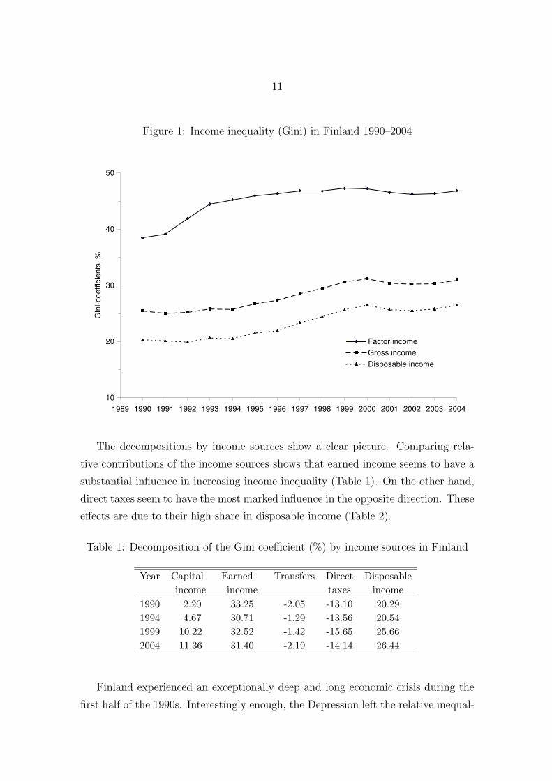
the trend in increasing inequality in factor income was stopped after 1997 (Figure 1).

Clearly public policy has some role in this. In light of the widely differing economic

conditions the time period 1990–2004 can been divided into time periods, the crisis

period 1990–1994, the period of economic recovery 1994–1999, with a sub-period of

rapid growth in 1996–1999, and the last period 1999–2004 while economic growth

slowed down. Comparison of decompositions of the Gini coefficient in 1990, 1994,

1999 and 2004 will be used to uncover some of the factors behind the recent and

rapid increase in income inequality.

3Capital income includes interest received less interest paid, rental income, dividends, pensions

and compensations based on private insurance, net imputed rents from owner-occupied dwellings

and realised capital gains. Income from self-employment accrues from agriculture, forestry and

firms. Employee income consists of cash wages and salaries, value of managerial stock options and

compensations in kind, deducting work expenses related to these earnings.4Current transfers received include benefits from unemployment and sick insurance and occupa-

tional and national old age, disability and unemployment pensions, child benefits, unemployment

and welfare assistance.5Current transfers paid include taxes paid on income and wealth and employee’s social insurance

contributions.

11

Figure 1: Income inequality (Gini) in Finland 1990–2004

10

20

30

40

50

1989 1990 1991 1992 1993 1994 1995 1996 1997 1998 1999 2000 2001 2002 2003 2004

Gin

i-coeff

icie

nts

, %

Factor income

Gross income

Disposable income

The decompositions by income sources show a clear picture. Comparing rela-

tive contributions of the income sources shows that earned income seems to have a

substantial influence in increasing income inequality (Table 1). On the other hand,

direct taxes seem to have the most marked influence in the opposite direction. These

effects are due to their high share in disposable income (Table 2).

Table 1: Decomposition of the Gini coefficient (%) by income sources in Finland

Year Capital Earned Transfers Direct Disposableincome income taxes income

1990 2.20 33.25 -2.05 -13.10 20.291994 4.67 30.71 -1.29 -13.56 20.541999 10.22 32.52 -1.42 -15.65 25.662004 11.36 31.40 -2.19 -14.14 26.44

Finland experienced an exceptionally deep and long economic crisis during the

first half of the 1990s. Interestingly enough, the Depression left the relative inequal-

12

Table 2: Mean disposable income (1000 e) by income sources in Finland

Year Capital Earned Transfers Direct Disposableincome income taxes income

1990 1.13 17.79 4.67 -5.92 17.661994 1.98 13.67 6.83 -5.90 16.571999 3.34 16.54 6.33 -7.02 19.192004 4.26 18.42 6.62 -7.15 22.14

ity seemingly unaffected. The change in Gini was insignificant, about one quarter of

a percentage point between 1990–1994. Unemployment rose more rapidly in the high

wage, male dominated sector, manufacturing. Since factor income was reduced, the

relative position of those who received stable income, such as pensioners, improved,

and automatic stabilisers operating through unemployment insurance improved the

relative income position of those receiving social transfers (Riihela et al. 2001).

However, the level of the public dept rose very rapidly, and this has been countered

by raising the tax rates on wage income. This clearly shows up in the data (Table 1).

In the period of economic recovery, 1994–1999, the value of overall Gini increased

remarkably by five percentage points. Although earned income has some contribu-

tion to this, capital income has been responsible for most of the increase in the Gini

coefficient. It would seem that change in the wage differentials has not been a major

factor for the substantial increase in inequality.6

6In the decade after 1979 the income inequality increased dramatically in the United Kingdom

after a relatively stable period of three decades, Johnson (1996). Over the last two decades wage

inequality and educational wage differentials have expanded markedly in the USA. These effects

show up particularly pronounced in the top income shares Atkinson (2003). There are several

explanations for this development. A popular one involves a positive productivity shock that

reward high skills relatively more than in the past. These skills are acquired by high education

levels and increased use of new information technology is frequently seen as a supplementary factor

in the skill-biased productivity change. In addition, some people see globalization of world trade

as an additional factor that adversely affects low-skill workers in the developed economies through

competition from emerging economies. If the composition of the labour force and labour supply

are held constant, the changes in the demand for labour are transmitted by either higher wages

or higher employment rates for high-skill workers. The latter effect shows up especially if low skill

workers are protected by minimum wages. In both cases high-skill workers increase their share in

wage income. This explanation has been extensively discussed and challenged by Atkinson (2000)

13

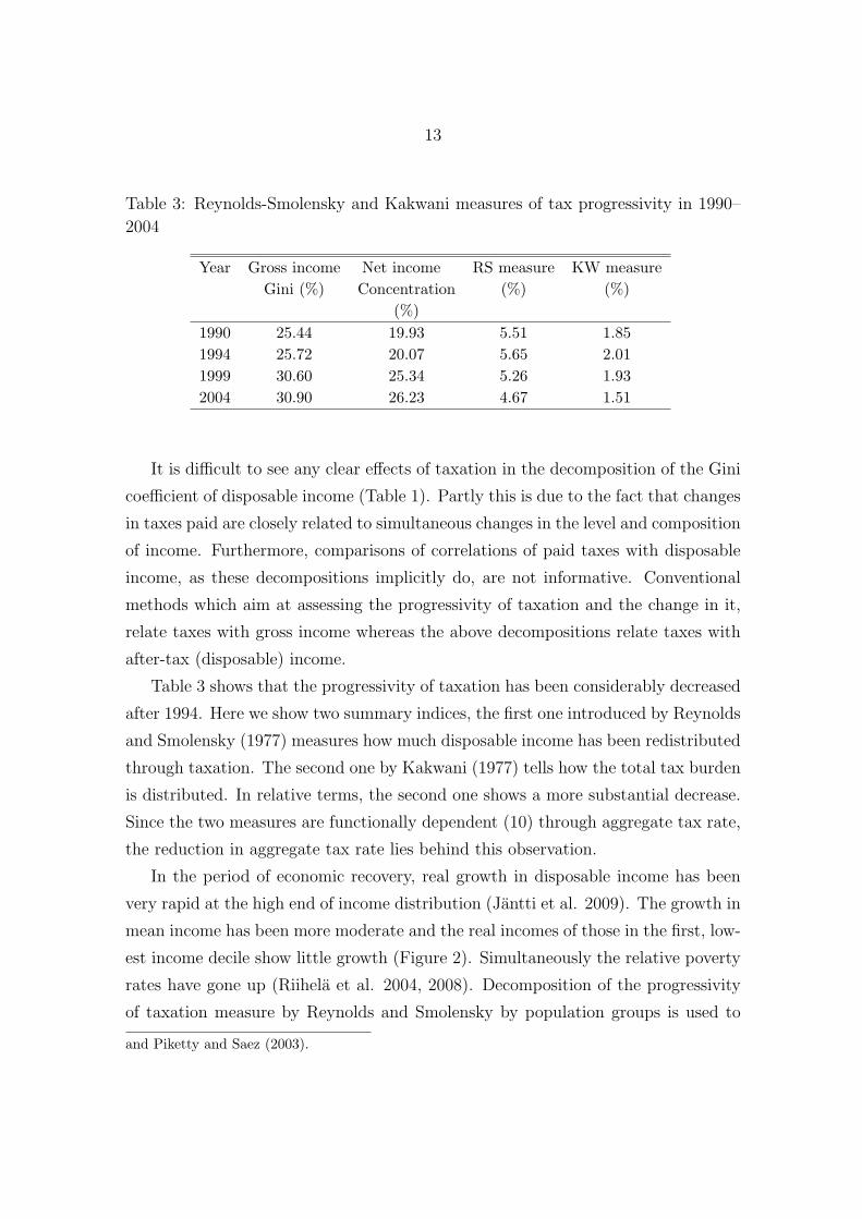
Table 3: Reynolds-Smolensky and Kakwani measures of tax progressivity in 1990–

2004

Year Gross income Net income RS measure KW measureGini (%) Concentration (%) (%)

(%)1990 25.44 19.93 5.51 1.851994 25.72 20.07 5.65 2.011999 30.60 25.34 5.26 1.932004 30.90 26.23 4.67 1.51

It is difficult to see any clear effects of taxation in the decomposition of the Gini

coefficient of disposable income (Table 1). Partly this is due to the fact that changes

in taxes paid are closely related to simultaneous changes in the level and composition

of income. Furthermore, comparisons of correlations of paid taxes with disposable

income, as these decompositions implicitly do, are not informative. Conventional

methods which aim at assessing the progressivity of taxation and the change in it,

relate taxes with gross income whereas the above decompositions relate taxes with

after-tax (disposable) income.

Table 3 shows that the progressivity of taxation has been considerably decreased

after 1994. Here we show two summary indices, the first one introduced by Reynolds

and Smolensky (1977) measures how much disposable income has been redistributed

through taxation. The second one by Kakwani (1977) tells how the total tax burden

is distributed. In relative terms, the second one shows a more substantial decrease.

Since the two measures are functionally dependent (10) through aggregate tax rate,

the reduction in aggregate tax rate lies behind this observation.

In the period of economic recovery, real growth in disposable income has been

very rapid at the high end of income distribution (Jantti et al. 2009). The growth in

mean income has been more moderate and the real incomes of those in the first, low-

est income decile show little growth (Figure 2). Simultaneously the relative poverty

rates have gone up (Riihela et al. 2004, 2008). Decomposition of the progressivity

of taxation measure by Reynolds and Smolensky by population groups is used to

and Piketty and Saez (2003).

14

examine the change in 1994–2004.

RS = G(x) − C(y, x) =∑

i

w(xi)(C(1i x, x) − w(yi)

w(xi)C(1i y, x)),

where w(xi) and w(yi), are the ith (before-tax) income deciles share in before-tax

and after-tax income, respectively.

Figure 2: Mean real disposable income in some income deciles in 1990–2004

1. declle

9. decile

10. decile

Top 1%

Total

Top 5%

0

20

40

60

80

100

120

140

1989 1990 1991 1992 1993 1994 1995 1996 1997 1998 1999 2000 2001 2002 2003 2004

1000 E

UR

To examine whether the change in progressivity can be localised to a particular

region in the income distribution, the population groups are defined on the basis

of before-tax (gross) income, taking the first nine income decile groups, 1,2,. . . ,9,

and dividing the top, 10. decile into two non-overlapping groups using the 99th

percentage point of the distribution. Therefore, the highest income group consists

of those in the top one per cent of the income distribution. Tables 4 and 5 show the

factors in the decomposition (14) in 1994 and 2004, respectively.

15

Table 4: Decomposition of the Reynolds-Smolensky progressivity by gross income

deciles in 1994

Income group Share in Concentration Share Concentration Contributionby Gross Gross in Gross coefficient after-taxincome income income in income

(%) (%) (%) (%)Top 1 per cent 3.72 99.14 0.84 99.14 0.6190-99 per cent 17.68 89.76 0.88 89.62 1.92

9. decile 14.17 70.36 0.93 70.28 0.668. decile 11.94 50.23 0.96 50.19 0.227. decile 10.56 30.17 1.00 30.14 0.016. decile 9.47 10.18 1.02 10.12 -0.025. decile 8.51 -9.81 1.05 -9.83 0.054. decile 7.58 -29.81 1.08 -29.86 0.193. decile 6.66 -49.77 1.13 -49.82 0.422. decile 5.64 -69.70 1.18 -69.77 0.72

First decile 4.07 -88.86 1.24 -88.94 0.88All 100.0 25.72 1.00 20.07 5.65

Table 5: Decomposition of the Reynolds-Smolensky progressivity by gross income

deciles in 2004

Income group Share in Concentration Share Concentration Contributionby Gross Gross in Gross coefficient after-taxincome income income in income

(%) (%) (%) (%)Top 1 per cent 7.03 99.40 0.87 99.42 0.9490-99 per cent 18.12 89.91 0.91 89.76 1.51

9. decile 14.13 70.36 0.96 70.30 0.398. decile 11.83 50.23 0.98 50.21 0.127. decile 10.36 30.21 1.00 30.17 0.006. decile 9.14 10.20 1.03 10.19 -0.025. decile 8.05 -9.78 1.05 -9.84 0.044. decile 7.02 -29.76 1.07 -29.80 0.153. decile 6.00 -49.71 1.11 -49.76 0.342. decile 4.90 -69.58 1.16 -69.70 0.55

First decile 3.44 -88.89 1.21 -88.93 0.66All 100.0 30.90 1.00 26.23 4.67

16

Our decomposition consists of a (before-tax) income share weighted average of

the terms, C(1i x, x) − (w(yi)/w(xi)) C(1i y, x), for each income group. We suggest

that, the concentration coefficients in before-tax income, C(1i x, x) and after-tax

income, C(1i y, x), can be interpreted to reflect “progressivity effects” within the

decile group, i. In Tables 4 and 5, C(1i x, x) − C(1i y, x) ≈ 0. In addition, there

seems to be little change in this difference over time. The coefficients (w(yi)/w(xi))

are more important to the analysis. They give the ratios of mean after-tax income

to before-tax income, in the different income deciles, where after-tax and before-tax

income are measured as shares in total after-tax and before-tax income, respectively.

Tables 4 and 5 show some increase in these coefficients at the high end of income

distribution. This means that after-tax income shares of those with high before-tax

income has increased over the comparison period more than their before-tax income

shares. In addition, we find that their share in before-tax income has increased

markedly in the time-period 1994–2004. For example, the top one per cent’s income

share has nearly doubled. These give the weights in the sum (14) which amplify the

decrease in progression which is mostly due to the after-tax and before-tax income

ratios at the high end of the income distribution.

This reflects the fact that measures of tax progressivity are sensitive both to

change in actual tax schedules and change in the distribution of before-tax income.

A fine example concerning the interplay of these two effects is the fact that the

product of these effects, w(xi)(C(1i x, x) − (w(yi)/w(xi)) C(1i y, x)), have actually

increased from 1994 to 2004 for those in the top one per cent before-tax income

group signalling more tax progressivity. This is in clear contrast to the case of the

8. and 9. decile groups and the 90–99 per cent group. At the very top we find an

increase in the progressivity of taxes.

However, since their share in before-tax income has nearly doubled, one would

expect that a clearly progressive tax schedule would result in more substantial rise

in the ratio of their relative shares in mean after-tax income to before-tax income

than the actual rise of three percentage points from 0.84 to 0.87. In our data the

“income growth for those in the top one per cent” has been much more rapid than

for the rest and has deformed the income distribution to the extent that the effect

due to actual tax schedules is masked by the distributional effect, “exception that

probes the rule”.7

7The quotation marks are used here to remind that we use gross section not panel data. In

17

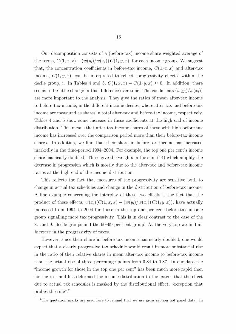
Table 6: Direct taxation and horizontal inequality in 1990, 1994, 1999 and 2004

Year Gini coefficient Concentration Horizontalin after-tax of after-tax inequalityincome (%) income (%) (%)

1990 20.29 19.93 0.361994 20.54 20.07 0.471999 25.66 25.34 0.322004 26.44 26.23 0.21

There has been a prominent change in the factor income in favour of capital, and

the Finnish firms have been exceptionally profitable during the last decade (Sauramo

2004 and Maliranta 2007). Presently, developments in capital income are the main

source for the increase in relative income inequality if the sources of factor income are

under consideration (Table 1). In addition, the main factor that has driven up the

top income shares in Finland since the mid 1990s is in an unprecedented increase in

the share of capital income. Top incomes are composed more and more of dividend

income (Jantti et al. 2009). The 1993 tax reform introducing dual income tax is

seen as one of the key factors responsible for this trend. The dual income tax treats

capital and wage income differently. In those income groups facing high marginal

tax rates in wage income, capital income is taxed using much lower rate.

One would expect that an introduction of dual income tax would result in sub-

stantial re-ranking after taxation. This should show up in the measure of horizontal

inequality. However, in contrast to expectations the data show relatively small ef-

fects in horizontal inequality of taxation (Table 6). In addition, there has been no

increase in these effects after 1994. A strong correlation of between before-tax in-

come level and share of capital income offers an explanation. This would in turn be

true if income shifting from wage income to dividend income becomes more popu-

addition we find that the concentration of after-tax incomes of the top one per cent group have

increased, signalling even more rapid change at the very top. Since the top income group has

no natural upper income bound these effects have very large standard errors and the results have

considerable year to year variation. Naturally there has been many small changes in actual tax

rates between 1994 and 2004. The tax rate of capital income was increased from 28 to 29 per

cent in 2000 and this may also have some influence at the very top end of income distribution (see

Figure 4, below).

18

lar with higher income. The 1993 Finnish tax reform, introducing the Nordic dual

income tax model, created strong incentives to shift wage income to capital income

for those in the highest marginal tax brackets (Lindhe et al. 2004; Pirttila and Selin

2006).

Figure 3: Composition of gross income and taxes in average values by gross income

deciles in 1994 and 2004

20

04

19

94

-75000

-50000

-25000

0

25000

50000

75000

100000

125000

150000

175000

200000

1 2 3 4 5 6 7 8 9 10Tot

al

1-9

deciles

Top 9

0-99

Top 1

%

EU

R

Earned income Capital income

Current transfers received State earned income tax

State capital income tax Property tax

Other current transfers paid

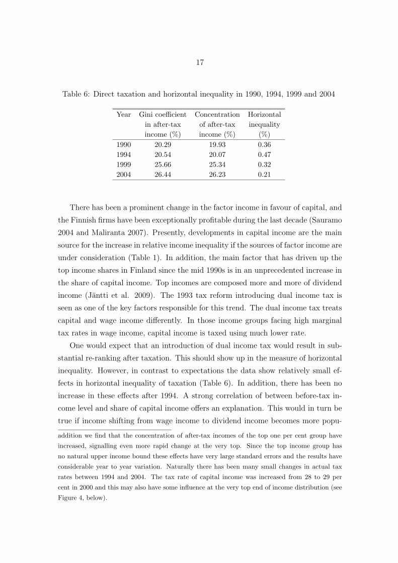
Figure 3 compares composition of gross income and taxes in average values by

the different income deciles in 1994 and 2004. The share of capital income increases

markedly moving up the income distribution in 2004. In the top one per cent the

share is particularly high, and in fact they pay most of their tax from capital income.

In 1994 the corresponding gradient is less pronounced. In addition, almost all real

income growth for those in the top one per cent in the distribution in 1994–2004

has accrued from capital income. This shows up in the distribution of total capital

19

Figure 4: Gross income deciles’ shares in earned and capital income in 1994 and

2004

Earned income (1994)

74.3

22.0

3.7

1. -9. deciles

Top 90-99

Top 1 %

Earned income (2004)

75.3

21.1

3.6

Capital income (1994)

13.0

22.7

64.3

Capital income (2004)

47.6

21.6

30.8

income between the income decile groups (Figure 4).

5 Conclusions

The paper has offered some observations and explanations for the recent evolution

of Finnish income inequality, focusing on the role of different sources of income and

in the progressivity of taxation. Total inequality rose significantly during the latter

part of the 1990s. The period of major income equalization from the early 1970s to

the mid 1990s has been reversed, taking the values of the Gini coefficient to levels

of inequality found 30 years ago.

20

Widening differentials in earnings seem to play a minor role in these develop-

ments even though the economy has experienced mass unemployment and dramatic

restructuring of the economy in the 1990s. As a general pattern, inequality rose

with growing capital income shares. In particular, among the well-to-do the share of

capital income grew most significantly during the late 1990s. The results show that

capital income although it appears to represent only 15 per cent of the total equiv-

alent household income makes by far the most significant contribution to overall

inequality. The decline in income progressivity since the mid 1990s and the un-

precedented increase in the share of capital income are important factors explaining

both the increase income inequality and top income shares in Finland.

The 1993 Finnish tax reform, introducing the Nordic dual income tax model, is

one of key factors responsible for this trend. Differential taxation of wage and capital

income created strong incentives to shift labour income to capital income for those

in the highest marginal tax brackets (Lindhe et al. 2004; Pirttila and Selin 2006).

In their study of the recent increase in US income inequality, particularly in the rise

of mega-incomes for the very top earners, Piketty and Saez (2003) conclude that

“the coupon-clipping rentiers have been overtaken by the working rich”. In Finland

the opposite seems true. Piketty and Saez (2003) give a central role to taxation,

executive compensation and shocks to capital returns.

Finland is a prime example of interaction of political and labour market power

(see e.g. Pekkarinen et al. 1992). The history of collective bargaining marks the

development of Finnish social security system. After the Economic Crisis of the

1990s, collective bargaining and political exchange in formulating economic policy

shifted their focus from expanding social security provisions to income taxes reduc-

tions and erosion in tax progressivity. The social norms and power have changed in

the Finnish society.

21

References

Atkinson, A.B. (1970), “On the measurement of inequality,” Journal of EconomicTheory, 2, 244–263.

Atkinson, A.B. (1997), “Bringing income distribution in from the Cold,” The Eco-nomic Journal, 107, 297–321.

Atkinson, A.B. (2000), “The changing distribution of income: evidence and expla-nations,” German Economic Review, 1, 3–18.

Atkinson, A.B. (2002),“Top incomes in the United Kingdom over the 20 th Century,”mimeo Nuffield College.

Atkinson, A.B. (2003), “Income inequality in OECD countries: Data and explana-tions,” CESifo Working Paper, 881.

Atkinson, A.B. and T. Piketty (2007), “Top Incomes over the 20 th Century: AContrast Between Continental European and English-Speaking Countries,”OxfordUniversity Press.

Jenkins, S.P. (1995), “Accounting for inequality trends; Decomposition analysis forthe UK 1971–86,” Economica, 62, 29–63.

Johnson, P. (1996), “The assessment: Inequality,” Oxford Review of Economic Pol-icy, 12, Spring, 1–14.

Jantti, M., M. Riihela, R. Sullstrom and M. Tuomala (2009), “Long term trends intop income shares in Finland,” forthcoming in the book (eds.) A.B. Atkinson andT. Piketty Top Incomes over the 20th Century: Volume II - A Global Perspective,Oxford University Press.

Kakwani, N.C. (1977), “Measurement of tax progressivity: An international com-parison,” Economic Journal, 87, 71–80.

Kalela, J., Kiander, J., Kivikuru, U., Loikkanen, H.A. and J. Simpura (eds.) (2001),“Down from the Heavens, up from the Ashes. The Finnish Economic Crisis of the1990s in the Light of Economic and Social Research,” VATT Publications, 27:6,Helsinki.

Kyyra, T. and M. Maliranta (2008), “The micro-level dynamics of declining labourshare: Lessons from the Finnish great leap,” Industrial and Corporate Change,doi:10.1093/icc/dtn006 (in press).

Lerman, R.I. and S. Yitzhaki (1985), “Income inequality effects by income source: Anew approach and applications to the United States,” The Review of Economicsand Statistics, 67, 151–156.

22

Lindhe, T., Sodersten, J. and A. Oberg (2004), “Economic effects of taxing differentorganizational forms under the Nordic dual income tax,” International Tax andPublic Finance, 52, 477–505.

Pekkarinen, J., M. Pohjola and B. Rowthorn (1992), “Social Corporatism,” Claren-don Press: Oxford.

Piketty, T. (2003), “Income inequality in France, 1901–1998,” Journal of PoliticalEconomy, 111, 1004–1042.

Piketty, T. and E. Saez (2003), “Income inequality in the United States 1913–1998,”Quarterly Journal of Economics, 118, 1–39.

Pirttila, J. and H. Selin (2006), “How successful is the dual income tax? Evidencefrom the Finnish tax reform of 1993,” Labour Institute for Economic Research,Working Papers, 223.

Reynolds, M. and E. Smolensky (1977), “Public Expenditures, Taxes and the Distri-bution of Income: The United States, 1950, 1961, 1970,” Academic Press: NY.

Riihela, M., R. Sullstrom, I. Suoniemi and M. Tuomala (2001), “Income inequality inFinland during 1990s,” in Kalela, J., Kiander, J., Kivikuru, U-M., Loikkanen, H.A.and J. Simpura, (eds.) Down from the Heavens, up from the Ashes. The FinnishEconomic Crisis of the 1990s in the Light of Economic and Social Research, VATTPublications, 27:6.

Riihela, M., R. Sullstrom and M. Tuomala (2004), “Recent trends in Economicpoverty in Finland,” in Vesa Puuronen (ed.) New Challenges for Welfare Society,Joensuu University Press.

Riihela, M., R. Sullstrom and M. Tuomala (2005), “Trends in top income shares inFinland,” Government Institute for Economic Research, Discussion Papers, 371.

Riihela, M., R. Sullstrom and M. Tuomala (2008), “Economic poverty in Finland1971–2004,” Finnish Economic Papers, 21, Number 1, Spring 2008.

Sauramo, P. (2004), “Is the labour share too low in Finland,” in Piekkola, H. andK. Snellman (eds.) Collective Bargaining and Wage Formation: Performance andChallences, Physica-Verlag.

Shorrocks, A.F. (1980), “The class of additively decomposable inequality measures,”Econometrica, 48, 613–625.

Shorrocks, A.F. (1982), “Inequality decomposition by factor components,” Econo-metrica, 50, 193–212.

Suoniemi, I. (2000), “Decomposing the Gini and the variation coefficients by incomesources and income recipients,” Labour Institute for Economic Research, WorkingPapers, 169.