Author's Accepted Manuscript

Tax Evasion and Public Expenditures on TaxRevenue Services in an Endogenous GrowthModel

Sifis Kafkalas, Pantelis Kalaitzidakis, VangelisTzouvelekas

PII: S0014-2921(14)00101-9DOI: http://dx.doi.org/10.1016/j.euroecorev.2014.06.014Reference: EER2614

To appear in: European Economic Review

Received date: 14 March 2013Revised date: 23 June 2014Accepted date: 26 June 2014

Cite this article as: Sifis Kafkalas, Pantelis Kalaitzidakis, Vangelis Tzouvelekas,Tax Evasion and Public Expenditures on Tax Revenue Services in anEndogenous Growth Model, European Economic Review, http://dx.doi.org/10.1016/j.euroecorev.2014.06.014

This is a PDF file of an unedited manuscript that has been accepted forpublication. As a service to our customers we are providing this early version ofthe manuscript. The manuscript will undergo copyediting, typesetting, andreview of the resulting galley proof before it is published in its final citable form.Please note that during the production process errors may be discovered whichcould affect the content, and all legal disclaimers that apply to the journalpertain.

www.elsevier.com/locate/eer

Tax Evasion and Public Expenditures on Tax Revenue Services in

an Endogenous Growth Model

Sifis Kafkalas, Pantelis Kalaitzidakis∗and Vangelis Tzouvelekas†

July 3, 2014

Abstract

This paper analyzes the relationship between tax evasion and the two main policy instruments af-

fecting tax compliance, namely, the announced tax rate and the share of tax revenues allocated to

tax monitoring mechanisms. For doing so, we adopt a simple one-sector endogenous growth model

modified under tax evasion following the Roubini and Sala-i-Martin (1993) analysis on income taxes

and tax compliance. Our model confirms Barro’s (1990) theoretical finding stating that the opti-

mal tax rate is equal to the elasticity of public capital. However, introducing a welfare function

where governments care also about the degree of fiscal corruption in the economy, the effective tax

rate is lower than the output elasticity of public capital in line with Futagami et al., (1993) and

Turnovsky (1997) theoretical results. Finally, our model is calibrated using data on tax evasion

from 35 OECD and 110 non-OECD countries for 2011. Simulation results suggest that both tax

evasion and output growth are decreasing with the share of tax revenues allocated to monitoring

expenses, while government’s utility maximization imply an announced tax rate lower from the

elasticity of public capital for both groups of countries.

Keywords: tax evasion, tax monitoring, effective tax rate.

JEL Codes: H21, H26, H54.

∗Department of Economics, University of Crete and Rimini Centre for Economic Activity.†Department of Economics, School of Social, Economics and Political Sciences, University of Crete, University

Campus, GR74100, Rethymno, Crete, Greece. Corresponding author: V. Tzouvelekas, Ph. +30.28310.77417, e-mail:v.tzouvelekas@uoc.gr.

1

1 Introduction

Income or corporate profit taxation matters for economic growth since taxes distort the accumula-

tion of private capital. Standard endogenous growth models suggest that the rate at which physical

capital is accumulated increases with their private return and, hence, high tax rates on income

or corporate profits are typically associated with low growth rates (Lucas, 1988; Rebelo, 1991).

However, taxation generates resources to finance the supply of the productive inputs provided by

the government including public goods and infrastructure. Since individuals are not charged by

their use of these public goods, government spending plays the role of an externality for the pri-

vate sector. Such an externality ends up being an engine of endogenous growth since the resulting

aggregate production function could display a high marginal productivity of private capital, which

permits perpetual capital accumulation (Barro, 1990; Turnovsky, 1997). Therefore, there is a ten-

sion between the role of taxation in creating disincentives for the accumulation of capital and the

role of the public spending financed by these taxes in raising the return from private capital.

An effective tax system must provide incentives to tax payers (individuals or corporate firms)

for tax compliance; otherwise, no taxes would be remitted voluntarily in a competitive economy.

Indeed empirical evidence suggests that tax evasion and fiscal corruption is a general and persistent

problem in virtually every country with serious negative consequences. Tax evasion constitutes a

sizable share of the shadow economy even in advanced industrialized countries around the globe.

Slemrod and Yitzhaki (2002) estimate that about the 17% of income taxes are unpaid in the US,

while the Tax Justice Network (2011) estimate that, on average, tax evasion rates in 119 developed

and developing countries around the world exceeds 50% of their healthcare spendings. Furthermore,

Schneider (2000) reports that the shadow output equals 39% of the actual magnitude of reported

GDP in developing countries, 23% in transition countries and 14% in OECD countries. Schneider

and Enste (2000) and Bajada (2003) suggest that the underground economy and the associated tax

evasion deepens recessions and increases the volatility of business cycles.

Starting from the seminal paper by Allingham and Sandmo (1972), a large amount of literature

relating to fiscal corruption and tax evasion has emerged aimed to analyze its determinants, magni-

tude, and welfare effects in both developed and developing economies (see Feige (1992) and Jung et

al., (1994) as well as the papers reviewed therein for a discussion on tax evasion and underground

economies). However, few papers analyze tax policies and evasion in a context of economic growth

models. Roubini and Sala-i-Martin (1995), assuming a positive relation between evasion and tax

rates, find that financial repression is associated with high tax evasion and low economic growth.

Lin and Yang (2001) extend the portfolio choice model in the presence of tax evasion from a static

to a dynamic setting suggests that aggregate output growth is convex with respect to the statutory

tax rate. However, their theoretical model neglects government externality assuming that public

goods and infrastructure do not affect the productivity of the private sector. Chen (2003), on the

other hand, integrated tax evasion into a standard AK model with public capital financed by in-

2

come taxation. In his model consumers first optimize their tax evasion levels, and then government

optimizes the statutory tax rate, tax auditing expenses and fines given the evasion level decided by

consumers. In contrast to Barro’s natural efficiency condition, his model suggests that the govern-

ment must set the statutory tax rate above its expenditure externality degree. Finally, Dzhumashev

and Gahramanov (2010) also adopted a standard endogenous growth model augmented with tax

evasion adjusted into a dynamic portfolio framework. Their model is similar to that by Lin and

Yang (2001) and suggsets that tax evasion rates are proportional to public spending externality.

Along these lines, we also adopt a standard one-sector endogenous growth model modified

accordingly to analyze how government decisions on the statutory tax rate and monitoring tax

compliance impact the rate of growth in the economy. Based on the theoretical framework of

Roubini and Sala-i-Martin (1995), we impose a tax evasion rate which is a positive function of the

announced tax rate and a negative function of tax revenues allocated for tax monitoring purposes.

In contrast to Chen (2003), we assume that tax revenues are allocated between tax monitoring and

public capital formation so that both expenditures are a constant share of total tax revenues. In

that way we ensure that Barro’s (1990) natural efficiency condition is satisfied in the steady-state,

i.e., the effective tax rate is indeed equal to the output elasticity of public capital. In addition, in the

public sector of the economy we assume that the government cares not only about the consumption

levels, but also about the degree of fiscal corruption as this is reflected by tax evasion rates in the

economy.

The above novel features of our model introduce a trade-off between tax evasion and output

growth rates, which is an important consideration for our social planner type government in de-

termining welfare maximizing policies. Using data from 35 OECD and 110 non-OECD countries

we first present empirical estimates of the tax evasion function at an aggregate level, confirming

Roubini and Sala-i-Martin (1995) assumption on the relation between the two policy variables and

evasion rates. These estimates are then used to assess the long-run effects of the two policy variables

on government’s utility maxmimization by simulating our model for the two groups of countries

separately.

The paper is organized as follows. Section 2 presents our model with effective taxation assuming

that individuals have the incentive to evade taxes and government allocates a constant share of tax

revenues to tax auditing. Section 3 determines the growth maximizing tax rate, while section 4

takes into consideration government’s perceptions about tax evasion. In section 5 our theoretical

model is calibrated using data from a sample of 35 OECD and 110 nn-OECD countries and section

5 concludes the paper.

3

2 A Growth Model with Effective Taxation

2.1 Model Description

We consider a closed economy populated by N identical agents who produce a single aggregate

commodity (Y ). Further, we assume that there is no population growth and that the labor force is

equal to the population, with labor supplied inelastically. Accordingly the ith representative firm

produces its output (Yi) using the following Cobb-Douglas production technology:

Yi = AKαi

(Kg

LLi

)(1−α)

(1)

where 0 < α < 1 is the output elasticity of private capital, A is a technological parameter, Ki

denotes the stock of private capital for firm i, Li the labor used by the representative firm, Kg

is the aggregate stock of public capital, and L is the total labor force. Therefore, each individual

firm benefits from an increase in economy-wide labor productivity (Kg

L ) triggered by a rise in the

stock of public capital. Under the above assumptions, the aggregate production function for our

hypothetical economy can be reduced to the standard AK model1 since

Y = AKαK(1−α)g (2)

Total output produced by individual firms in the economy can be either consumed or trans-

formed to private or public capital. Each type of capital accumulates as follows:

K = I − δkK (3)

and

Kg = G− δgKg (4)

where I, G denote gross private and public investment, and δk, δg the constant depreciation rates

for private and public capital, respectively.

The government finances its total expenditures through tax revenues collected via a tax rate

τ imposed on total output produced by firms. However, if tax evasion is allowed, the effective

tax rate is different from the official tax rate announced by the government. A history of public

waste and inefficient provision of public services may lead individual firms less willing to pay taxes.

Further, government may have access to an inferior technology for tax collection that detects tax

evaders or even the legislation framework is not strict in prosecuting evaders. Hence, government

may announce a tax rate τ , but individual firms may pay taxes that correspond to a lower actual

or effective tax rate denoted by τ e.

1Under the Cobb-Douglas assumption for the production technology our results will be comparable with therelevant literature on optimal taxation, triggered by the seminal work of Barro (1990).

4

The difference between the announced and the effective tax rate is the tax evasion rate (τ −τ e) which, following Roubini and Sala-i-Martin (1995), is assumed to be a negative function of

government expenditure allocated to tax monitoring, and a positive function of the announced

tax rate2. Public expenditures for improving the technology and, thus, the efficiency of the tax

collection mechanism may improve the ability of tax authorities to detect tax evaders and control

tax evasion. On the other hand, the incentive for tax compliance may decrease as the announced

tax rate increases because, for a given state of tax monitoring, the marginal benefit of tax evasion

increases.3 Therefore, it holds that:

τ − τ e = h (τ , μ) (5)

with∂h(τ , μ)

∂μ< 0 and 0 <

∂h(τ , μ)

∂τ< 1

where τ e ≤ τ , and μ = MT is the share of tax revenues, i.e., T = τ eY , that goes to monitor tax

compliance, M . The share of tax revenues directed towards gross public investment is (1 − μ),

leading to:

M = μτ eY and G = (1− μ) τ eY (6)

which imply that central government’s budget constraint is given from the following relation:

T = M +G = τ eY (7)

In the consumption sector of our economy consumers derive utility only from the consumption of

the aggregate commodity produced. Assuming a constant elasticity formulation, the representative

infinite lived consumer has the following lifetime utility function:

U =

ˆ ∞

0e−ρt

(c(1−θ)

1− θ

)dt (8)

where ρ > 0 is the rate of time preference, c = CL is the per capita consumption, and θ > 0 is the

reciprocal of the intertemporal elasticity of substitution.

Finally, the disposable income for the representative consumer can be either consumed or in-

vested for private capital accumulation

(1− τ e)y = c+ k + δkk, (9)

2In Appendix A.1 we provide a proof of these monotonicity properties of the tax evasion function under a morestructural optimizing behaviour by individual firms

3It should be noted here, that in the Allingham and Sandmo (1972) model the result of a tax rate change onevasion is ambiguous due to the opposite income and substitution effects. Yitzhaki (1974), on the other hand, provedthat if the penalty of tax evasion is exclusively on the evaded tax, then the substitution effect is absent and theincrease on tax rate decreases evasion. However, empirical evidence suggest that higher statutory tax rates encouragerather than repress tax evasion (see Dhami and al-Nowaihi, 2007 for details).

5

or, using (2),

k = (1− τ e)Akαk(1−α)

g − c− δkk (10)

where y = YL is the total output per worker, and k = K

L , kg =Kg

L are the private and public capital

to labor ratio, respectively.

2.2 Model Solution

The infinite horizon utility maximization problem for the representative consumer is given from

max U =

ˆ ∞

0e−ρt

(c(1−θ)

1− θ

)dt

s.t. k = (1− τ e)Akαk(1−α)

g − c− δkk

with the present value Hamiltonian

H = e−ρt

(c(1−θ)

1− θ

)+ q

[(1− τ e)Ak

αk(1−α)g − c− δkk

](11)

where q is the present value shadow price of private capital stock in terms of utility.

The first-order conditions for c and k are given from the following relations:

∂H

∂c= 0 ⇒ e−ρtc−θ = q (12)

∂H

∂k= −q ⇒ −q = q

[α (1− τ e)Az

(1−α) − δk

](13)

where z =Kg

K is the ratio of public to private capital in the economy.

Eliminating the shadow price of private capital stock from the above system we obtain:

c =1

θ

[α (1− τ e)Az

(1−α) − δk − ρ]

(14)

Since in the steady-state all the basic variables of our model grow at the same rate (i.e., y =

c = k = kg = gy), equations (2), (4) and (6) imply:

kg = (1− μ)τ eAz−α − δg = gy (15)

Solving (15) with respect to z, substituting it into (14) and assuming that δk = δg = δ, the

steady-state growth rate of our economy is:

(θgy + δ + ρ)(gy + δ

)( 1−αα

)= αA

1α (1− τ e)

[(1− μ)τ e

]( 1−αα

)(16)

This relation reveals that both the announced tax rate and the share of tax monitoring expenses

6

impact the long-run growth rate of the economy. In the next section, we address the question

of growth-maximizing policies by considering the growth-maximizing values of these two policy

variables.

3 Growth-Maximizing Policies

The determination of the growth-maximizing policies is achieved in two steps: first, the planner

determines the growth maximizing steady-state statutory tax rate for a given allocation of govern-

ment expenditure, and then derives the growth-maximizing steady-state share of tax monitoring

expenditure at the given optimal tax rate. In our framework, taxation affects the growth of the

economy through two channels. While taxation affects negatively the marginal product of private

capital as it absorbs resources from the private sector of the economy, government expenditure for

public capital formation, collected through tax revenues, increases the productivity of labor. At

low values of τ , the positive effect of government expenditure dominates, and therefore the growth

rate of the economy rises with the announced tax rate. At higher tax rates, the negative effect of

taxation eventually dominates, and the growth rate declines as τ further rises. The statutory tax

rate that maximizes the growth rate of the economy is the one that equates the marginal cost of

government expenditure to its marginal benefit. The following proposition determines the growth

maximizing tax rate.4

Proposition 1 The statutory tax rate that maximizes the growth rate of the economy is

τ = 1− α+ h (τ , μ) ⇒ τ e = 1− α

Proof. From relation (16) we calculate the partial derivative of the growth rate with respect to

the announced tax rate and we set it equal to zero to provide the result.

This result is similar to the typical finding obtained by standard endogenous growth models,

which states that the growth maximizing tax rate is equal to the elasticity of public capital in the

aggregate production function (see, among others Barro, 1990). Here, Proposition 1 shows that,

in the presence of a tax auditing cost, the optimal statutory tax rate is greater than the elasticity

of public capital in the aggregate production function. However, the optimal announced tax rate

has to be such that the effective tax rate is equal to the elasticity of public capital in the aggregate

production function.

Barro’s (1990) theoretical finding on optimal taxation has received considerable attention in

the literature. While most of the literature supports Barro’s (1990) result, some findings deviate,

suggesting a growth maximizing effective tax rate greater than the output elasticity of public

capital. The interpretation of these conflicting findings is not always convincing. Trying to gain a

4In Appendix A.2 we present the result for a CES production technology.

7

better understanding of this puzzle, we compare our analysis with Chen (2003) who uses a similar

approach with ours, suggesting though that the growth maximizing effective tax rate should be

greater than the corresponding elasticity of public capital.

Taking a closer look into these two models, we see that the essential difference between them

is the way that tax monitoring expenses enter into government’s budget constraint. As relation

(6) shows, in our model tax revenues are allocated between tax monitoring and public capital

formation so that both expenditures are constant shares of total tax revenues. In contrast, Chen

(2003) defines tax monitoring expenditure as a constant share of total income (output). In order to

show that this assumption is responsible for the conflicting results on growth maximizing taxation,

we embody Chen’s (2003) assumption into our model. This modifies equation (6) as follows:

M = λY and G = (τ e − λ)Y (17)

where 0 < λ < τ e is a constant denoting the share of total output allocated for tax auditing

purposes.

Notice that equation (16), the steady-state growth rate of the economy, under both assumptions

on the share of tax monitoring expenses, can be written as a general function of μ and τ e,

gy = f

((1− τ e)

[G

Y

] 1−αα

)=

⎧⎪⎪⎨⎪⎪⎩f

((1− τ e)

[(1− μ)τ e

]1−αα

)under relation (6)

f

((1− τ e)

[τ e − λ

] 1−αα

)under relation (17)

(18)

since the growth rate of the economy is monotonic to the expression (1− τ e)[GY

] 1−αα . The first term

of this expression captures the negative effect of taxation on growth through its negative impact on

the marginal product of private capital. The second term captures the positive effect of taxation

on growth through higher public expenditures for public capital formation.

Assuming that tax monitoring expenses are a constant share of total output (i.e., relation (17)),

the following proposition holds:

Proposition 2 If tax monitoring expenditures are a constant share of total income, λ, then the

effective tax rate maximizing the growth rate of the economy is

τ e = 1− α (1− λ) > (1− α)

Proof. From (18) we observe that maximizing the steady-state growth rate with respect to the

effective tax rate is equivalent to maximizing (1− τ e) (τ e − λ)1−αα with respect to the effective tax

rate.

The above proposition implies that, when tax monitoring expenditure is proportional to total

income rather than to total tax revenues, the growth-maximizing effective tax rate is greater than

8

the output elasticity of public capital. When tax revenues are allocated proportionally among tax

monitoring and public capital formation, an increase in the tax revenues by one dollar will raise

government expenditure for public capital formation by less than a dollar. However, when the

tax monitoring expenditure is a constant share of output, the whole increase in the tax revenues

is allocated exclusively for public capital formation. In the latter case the marginal benefit of an

increase in the effective tax rate is greater than in the former case, leading to a higher growth-

maximizing effective tax rate.

4 Growth vs Welfare Maximizing Policies

In order to analyze the utility maximizing policies, we determine first the equilibrium path of

consumption and, then, we calculate the steady-state value of lifetime utility as a function of the

two policy variables (τ and μ). Consumption grows at a rate gy(τ , μ) with its time path given by:

ct = c0egy(τ ,μ)t (19)

where c0 is the initial per capita consumption that is determined endogenously. Dividing both sides

of equation (10) by k, we get:

k

k= (1− τ e)Az

(1−α) − c0k0

− δ

where k0 is the initial stock of private capital per worker in the economy.

Then, solving (15) for z and substituting into the above equation, we obtain the following

expression for the initial per capita consumption:

c0(τ , μ) =

[1

α

(θgy(τ , μ) + δ + ρ

)−(gy(τ , μ) + δ

)]k0 (20)

Substituting the optimal ct into the lifetime utility function in (8) we obtain the lifetime steady-

state utility function from the following relation:

V (τ , μ) =c(1−θ)0

(1− θ)[ρ− gy(τ , μ)(1− θ)

] (21)

where gy(·) and c0(·) are given from equations (16) and (20), respectively. As it can be easily shown,

lifetime indirect utility is monotonically increasing in gy which implies that growth maximizing

policies are also utility maximizing policies.

Given the growth maximizing effective tax rate, the growth rate of the economy becomes a

decreasing function of the share of government expenditure for tax monitoring. This result is not

surprising since tax monitoring absorbs productive resources to reduce tax evasion that could be

9

costlessly achieved by an increase in the announced tax rate. A reduction in the share of public

expenditure allocated to tax monitoring raises the steady-state growth of the economy but, at the

same time, the announced tax rate has to increase for the effective tax rate to remain at the growth

maximizing level. As a result, the tax evasion rate increases.

However, this is not always appropriate as tax evasion introduces fiscal corruption in the econ-

omy, which, in turn, exerts adverse effects on social welfare. Empirical evidence in both developed

and developing countries suggests that in economies with high tax evasion rates there is also signif-

icant corruption. This is related either to the attitude of bureaucrats who control public services

provision or to the dishonesty of tax inspectors who solicit bribes not to report tax evasion. Both

types of corruption have a significant effect on the equity and the efficiency of any economic system

(Chander and Wilde, 1992; Hindriks et al., 1999; Sanyal et al., 2000; Slemrod and Yitzhaki, 2002).

To work out this problem, we introduce a social planner type government that cares not only

about the consumption of the aggregate commodity produced, but also about the degree of fiscal

corruption in the economy as this is captured by tax evasion rates. Following Brock and Taylor

(2005), we assume that government’s objective function has the following constant elasticity form:

Us =

ˆ ∞

0e−ρt

(c(1−θ)

1− θ− h(τ , μ)γ

γ

)dt (22)

where γ ≥ 0 is the relative weight factor of tax evasion in the instant utility function. As γ decreases

the more important tax evasion is for the government. The above formulation implies that steady-

state value of government’s objective function is decreasing and quasi-concave in the rate of tax

evasion:

Vs (τ , μ) =c(1−θ)0

(1− θ)[ρ− gy(τ , μ)(1 − θ)

] − h(τ , μ)γ

ργ(23)

From the above it can been seen that maximizing government’s objective function implies a

trade-off between the growth rate of the economy and the rate of tax evasion. A decrease in

the share of tax monitoring expenditures increases the growth rate of the economy, the path of

consumption shifts upwards and, thus, government’s utility tends to rise. At the same time, the

decrease in the share of tax monitoring expenses accompanying an increase in the announced tax

rate, increases the rate of tax evasion, which tends to decrease the utility of the government. In

this case, a welfare maximizing share of tax monitoring may exist, since the two effects of tax

monitoring expenditures in government’s utility are of opposite directions.

Maximizing the above steady-state value of government’s objective function with respect to the

share of tax monitoring and the announced tax rate leads to the following optimality conditions:

∂Vs(τ , μ)

∂μ= 0 ⇒ ∂Vs(τ , μ)

∂gy(τ , μ)

∂gy(τ , μ)

∂μ=

∂Vs(τ , μ)

∂h(τ , μ)

∂h(τ , μ)

∂μ(24)

10

and

∂Vs(τ , μ)

∂τ= 0 ⇒ ∂Vs(τ , μ)

∂gy(τ , μ)

∂gy(τ , μ)

∂τ=

∂Vs(τ , μ)

∂h(τ , μ)

∂h(τ , μ)

∂τ, (25)

The expression in (24) is a typical optimality condition equating the marginal cost of an increase

in tax monitoring expenditures with their marginal benefits measured in terms of government’s

utility. The marginal cost refers to the decrease of output growth and therefore, the time path

of consumption, while the marginal benefits refers to the improvement of tax compliance and the

associated decrease in the degree of fiscal corruption in the economy. In a similar manner, (25)

provides the same result for the announced tax rate. Using both relations, the following proposition

holds.

Proposition 3 The effective tax rate that maximizes social welfare is lower than the output elas-

ticity of public capital:

τ e < (1− α)

Proof. Dividing equation (24) by (25) and using (18) yields:

∂gy(τ ,μ)∂μ

∂gy(τ ,μ)∂τ

=

∂h(τ ,μ)∂μ

∂h(τ ,μ)∂τ

⇒∂

((1− τ e)

[(1− μ) τ e

] 1−αα

)/∂μ

∂

((1− τ e)

[(1− μ) τ e

] 1−αα

)/∂τ

=

∂h(τ ,μ)∂μ

∂h(τ ,μ)∂τ

⇒ τ e = (1− α) +(1− α) (1− τ e) τ e

(1− μ)

∂h(τ ,μ)∂τ

∂h(τ ,μ)∂μ

< (1− α) (26)

which provides the result.

This result is similar to those provided by Futagami et al., (1993) and Turnovsky (1997). These

two papers derive, in the case of the decentralized economy, a growth-maximizing tax rate equal

to the output elasticity of public capital. However, in the social planer’s case, the optimum tax

rate is less than the output elasticity of public capital due to an externality associated with the

accumulation of public capital. As a result, Barro’s (1990) finding that the growth-maximizing tax

rate also maximizes the steady-state lifetime utility does not hold when public capital rather than

public expenditure enters into the production function. Proposition 3 derives a similar result with

respect to our effective tax rate, even though the mechanism generating our result is different from

that of Futagami et al., (1993) and Turnovsky (1997). In our model, we employ a social welfare

function that introduces a trade-off between output growth and tax evasion, leading to an optimum

effective tax rate lower than the one that maximizes the growth rate of the economy.

However, the above result does not apply when the government is a revenue maximizing

Leviathan diverting taxes for it’s own selfish purposes (Edwards and Keen, 1996; Keen and Kotso-

giannis, 2002). Keeping the same assumptions concerning the economy, in every period government

11

will choose an effective tax rate that maximizes the following:

Tt = τ eYt−1 exp(gy)

The first order condition for a maximum requires that

∂Tt

∂τ e= 0 ⇒ ∂gy

∂τ e= − 1

τ e

This result implies that a Leviathan type of government in maximizing it’s total tax revenues

will choose a tax rate such that the derivative of the growth rate with respect to the effective tax

rate is negative. This in turn suggests that the effective tax rate is higher than the elasticity of

public capital, i.e., τ e > 1− α, as Proposition 1 implies.

5 Model Simulation

5.1 Estimation of Tax Evasion Function

Before simulating the model, to qualitatively illustrate the long-run effects of the two policy vari-

ables (i.e., announced tax rate and tax monitoring expenses), we specify a functional form for the

econometric estimation of the tax evasion function in (5). Our theoretical framework implies that

the tax evasion rate is directly affected by these two policy variables. However, plenty of empirical

evidence, using experimental or survey data, suggests that tax compliance goes beyond the tradi-

tional deterrence model. Specifically, it explains tax morale as a more complicated process between

taxpayers and the government formed by the prevailing sociological, cultural or economic conditions

in every economy. In particular, Sandmo (2006) argues that the economic structure affects directly

evasion rates as income generated in the industrial sector can be less easily evaded than that in

the service sector. In contrast, Slemrod et al. (2001) argues that intrinsic motivation formed by

education or socialization of individuals is a key determinant of tax compliance rates, exogenous

to government policy. Further, Feld and Tyran (2002) and Alm and Togler (2006), suggest that

social norms about tax morale serve as the main determinant of evasion rates. Finally, Feld and

Frey (2007) argue that the contractual relationship between tax payers and tax authorities has

important implications on tax compliance.5

Unfortunately, detailed aggregate data for all these factors, underlined by the relevant literature

as important determinants of tax evasion rates, are not available from any known source for a broad

set of countries. Therefore, to lessen the potential biases arising from these omitted explanatory

variable, in approximating empirically tax evasion function we adopt the Jorgenson and Nishimizu

(1978) bilateral approach modified for our empirical context. Specifically, we distinguish between

two groups of countries, i.e., OECD and non-OECD, assuming that each one of these groups exhibits

5Sandmo (2006) and Bajada and Schneider (2005) provide a detailed review of the empirical and experimentalstudies on the determinants of tax evasion rates.

12

different structure of the tax evasion function and different impact of the two policy variables have

on tax compliance.6 Since the economic, institutional and social environment is different between

these two groups, we may reasonably assume that the direct impact of the two policy variables on tax

compliance will also differ between the two country groups. Allowing, for group specific marginal

effects of the two policy variables, we indirectly incorporate those sociological, institutional or

economic factors that cannot be measured directly at an aggregate level.7 In addition, we include

in the tax evasion function the degree of government effectiveness by following the empirical study

on shadow economies by Schneider et al., (2010) to capture the effects of the quality of tax auditing

mechanism and regulatory framework. Finally, real GDP per capita is included as an explanatory

variable capturing income differences among countries in the sample. Even within the same group,

income differences may affect tax compliance behaviour by individual firms.8 Under the above

assumptions, the bilateral tax evasion function that is estimated econometrically has the following

form:

lnhi = ln β0 + βg lnGEi + βr lnRGDPi + βτj ln τ i + βμj lnμi + εi (27)

where i denotes countries, j = 1, 2 the two groups of countries (OECD and non-OECD countries)

defined in the bilateral structure of tax evasion function, h is the tax evasion expressed as the share

of tax revenues that are evaded, GE is an index capturing perceptions on the quality of regulatory

framework and tax auditing mechanism, RGDP is the real per capita GDP, τ is the announced

tax rate by the government, μ is the share of tax revenues that goes for monitoring tax compliance,

εi depicts a symmetric and normally distributed error term, i.e., εi ∼ N(0, σ2

ε

), which represents

left-out explanatory variables and measurement errors in the dependent variable, and βτj = βτDj

and βμj = βμDj are the bilateral coefficients with Dj = 1 for country belonging to group j and

Dj = 0 otherwise.

The necessary data for the econometric estimation of (27) are obtained from the Tax Justice

Network covering 35 OECD and 110 non-OECD countries for the year 2011.9 This report provides

6We are indebted to a reviewer of an earlier version of this paper for suggesting the distinction between developedand developing countries in approximating empirically tax evasion function.

7Initially, we have tried to fit a multilateral structure in the econometric estimation of (5) using Barro andLee (2010) country grouping (i.e., Advanced Economies, South and Central America and the Caribbean, Asia andthe Pacific, North Africa and Middle East, and Sub-Sahara Africa), but the results were unsatisfactory. We thenfollowed Simar (2003) approach to detect the potential outliers inside the groups and more accurate define country-grouping but it turned that the best econometric results were obtained from the bilateral structure. Without any apriori knowledge on the factors influencing tax compliance rates and how these differ among countries, this ratherblind process cannot provide satisfactory results. Only distinct differences on the social, institutional and economicenvironment that clearly exist between OECD and non-OECD countries can provide a good fit of the tax evasionfunction.

8We have also tried to include more variables suggested by Schneider et al., (2010) like, fiscal freedom, regulatoryquality or the share of direct taxes to total tax burden but we didn’t get statistically significant parameter estimates.

9The 35 OECD countries in the sample are: Australia, Austria, Belgium, Canada, Chile, Czech Republic, Denmark,Estonia, Finland, France, Germany, Greece, Hungary, Iceland, Ireland, Israel, Italy, Japan, Luxemburg, Mexico,Netherlands, New Zealand, Norway, Poland, Portugal, Saudi Arabia, Slovakia, Slovenia, South Korea, Spain, Sweden,Switzerland, Turkey, UK, USA. Accordingly, the 110 non-OECD countries are the following: Albania, Algeria,Angola, Argentina, Armenia, Azerbaijan, Bahamas, Bahrain, Bangladesh, Belarus, Belize, Benin, Bhutan, Bolivia,Bosnia, Botswana, Brazil, Bulgaria, Burkina Faso, Burundi, Cambodia, Cameroon, Canada, Cape Verde, Central

13

data on overall tax burden (including both direct and indirect taxes), tax revenues lost as a result

of the shadow economy and the share of government spendings to GDP.10 Government spending

is used as a proxy of tax revenues in constructing the dependent variable. Monitoring expenses

are not available and are proxied indirectly using data on public expenditures published by the

Global Development Network Growth Database published by the World Bank. Spendings on public

infrastructure, health care, military and education expenses were subtracted from total government

spendings to develop a proxy of monitoring expenses for tax evasion. Since specific data on tax

services and monitoring infrastructure are not available from any known source for this broad set of

countries, the proposed variable is constructed residually from all other public spendings to serve

as a reasonably proxy of the share of tax revenues allocated in tax auditing mechanisms.

The index of government effectiveness is obtained from the Worldwide Governance Indicators

also published by the World Bank.11 The index captures perceptions of the quality of public ser-

vices, including tax auditing mechanisms, the quality of policy formulation and implementation

and the creditability of government’s commitment to such policies. This index ranges between -2.5

and 2.5 with higher scores corresponding to more effective central government. However, the index

is scaled to the 0-100 range to allow it’s logarithmic transformation in the econometric estimation

of (27). Finally, real GDP per capita, at constant 2007 US dollars, is obtained from the Penn

World Tables Ver 8.0. Summary statistics of these variables are provided in the upper panel of

Table 1. On average, tax evasion rates are very close between the two groups with OECD coun-

tries exhibiting a slightly lower mean value (6.42% and 7.01% for OECD and non-OECD countries,

respectively). However, the range of this mean values differs significantly between the two subsam-

ples. Specifically, in OECD countries tax evasion rates range between 11.64 and 1.19%, whereas in

non-OECD countries the corresponding range is considerably higher, 19.23 and 1.11% indicating

that in some countries evasion rates are a major problem. On the other hand, the average values

of both the announced tax rate and the share of government spendings allocated to tax auditing

mechanisms, exhibits considerable differences between the two groups. In particular, statutory

tax rate and monitoring expenses are 34.36% and 12.19% respectively, for OECD countries, while

the corresponding figures for the sample of non-OECD countries are 18.18% and 6.23%. Finally,

perceptions about government effectiveness are considerably higher in OECD countries indicating

a better quality of tax auditing mechanisms and regulatory framework.

African Republic, Chad, China, Colombia, Comoros, Costa Rica, Cote d’Ivoire, Croatia, Cyprus, Congo, DominicanRepublic, Ecuador, Egypt, El Salvador, Guinea, Ethiopia, Fiji, Gabon, Gambia, Georgia, Ghana, Guinea, Guinea-Bisau, Guyana, Haiti, Honduras, India, Indonesia, Iran, Jamaica, Jordan, Kazakhstan, Kenya, Kuwait, Kyrgyzstan,Laos, Latvia, Lebanon, Lesotho, Liberia, Libya, Lithuania, FYROM, Madagascar, Malawi, Malaysia, Maldives,Mali, Malta, Mauritius, Mongolia, Morocco, Namibia, Nepal, Nicaragua, Oman, Pakistan, Papua, Paraguay, Peru,Philippines, Qatar, Republic of Congo, Romania, Russia, Senegal, Sierra Leone, Singapore, Solomon, South Africa,Sri Lanka, Suriname, Syria, Taiwan, Tajikistan, Tanzania, Thailand, Trinidad, Tunisia, Uganda, Ukraine, UnitedArab Emirates, Uruguay, Venezuela, Vietnam, Yemen, and Zambia.

10See http://www.taxjustice.net. In summary, the absolute size of the shadow economy in each country is calculatedusing recently reported data by the World Bank. Then, assuming that the economic activity in the shadow economyin each country is tax evading they calculate the amount of taxes lost based on the average tax burden in each country.

11Both World Bank databases are available on line at: web.worldbank.org.

14

The lower panel of Table 1 presents the parameter estimates of the bilateral tax evasion function.

The overall fit of the econometric model is satisfactory as the adjusted-R2 is sufficiently large for a

cross-section setting (0.75). Parameter estimates of the two policy variables are having the correct

sign and size as the announced tax rate increases tax evasion, while monitoring expenses decreases

willingness to evade taxes. This is true for both group of countries. First, for the group of OECD

countries, the corresponding tax evasion elasticity values are 0.9026 and -0.1230 for announced

tax rate and tax monitoring expenses, respectively. On the other hand, in non-OECD countries

tax evasion is more sensitive to changes in both policy variables as the respective point elasticity

estimates are greater in absolute value, 1.1087 and -0.1994 for announced tax rate and tax auditing

expenses, respectively. Government effectiveness affects positively tax compliance as the better

quality of the provided public services including tax auditing mechanisms lessens tax evasion among

individuals. Finally, real GDP per capita seems to impact negatively tax evasion implying that as

per capita income rises consumers’ willingness to evade taxes decreases.

5.2 Welfare Maximizing Effects of the Two Policy Variables

Next, we assign specific values to the structural parameters of (16) to simulate the long-run effects

of the two policy variables on welfare maximization (see Table 2). First, the output elasticity of

private capital in the aggregate production function in (1) is set so that the optimal statutory tax

rate to be close to it’s observed value in the sample.12 Table 1 presents the average tax burden for

the group of OECD countries is 34.36% while that for the group of non-OECD countries is only

18.18%. Thus, in the model simulation we set α = 0.65 for the OECD countries and α = 0.80 for

the non-OECD countries. Since these values are arbitrarily chosen, we also perform a sensitivity

analysis taking into account two more values, within a 0.10 range during model simulation (0.55

and 0.75 for OECD countries and 0.70 and 0.90 for non-OECD countries).13 The depreciation

rate (δ) for capital stock is assumed to last 10 years on average. Following Acemoglou and Zilboti

(2001), we assume a constant annual depreciation rate of physical capital at 8.0%. We also used

depreciation rates of 4% and 6% with the simulation to test the robustness of our results and we

find no significant differences compared with those reported here.

Following Jones et al., (1993) and Dzhumashev and Gahramanov (2010), the discount rate of

consumer preferences is set at ρ = 0.020. Accordingly, the reciprocal of the intertemporal elasticity

of substitution was set at θ = 1.500 following Chen (2003). The steady-state growth rate, gy, is set

to 3.0% for the group of OECD countries and 2.0% for the group of non-OECD countries. Both

growth rate values are obtained as the average values of the 1970-2007 period using Penn World

Tables. Finally, the coefficient of productivity in (2) is set to A = 0.3327 and A = 0.2432 so that

the steady-state output growth rate equals 3.0% and 2.0% for OECD and non-OECD countries,

12Dzhumashev and Gahramanov (2010) simulating the Australian economy set α = 0.70 implying an optimal taxrate of 30%, while Chen (2003) assigned a higher value, α = 0.90 in order to get an optimal tax rate within reasonablevalues as according to his model announced tax rate is higher than (1− α).

13This is a common problem in endogenous growth models.

15

respectively. This is calculated by solving (16) for each group of countries assuming a steady-state

rate of growth in aggregate output of 3.0% or 2.0% in the absence of tax evasion, i.e., μ = 0 and

τ = τ e.

Using these parameter values and the econometric estimates of the tax evasion function in (27),

the announced tax rate is calculated from relation (26) under different values of tax monitoring

expenses for both groups of countries. Specifically, a pace of 0.25% in the share of monitoring

expenses is used during computations. Then, tax evasion levels, τ − τ e, and effective tax rate, τ e,

are calculated using the tax evasion function and it’s corresponding parameter estimates. Plugging

these values into the equilibrium condition in (16) we obtain the steady-state output growth rates

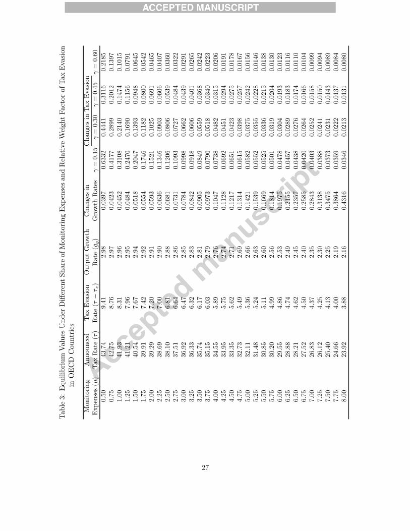
in the presence of tax evasion for both groups of countries. The obtained equilibrium values of

monitoring expenses, announced tax rate, tax evasion and output growth are reported in Tables 3

and 4 for OECD and non-OECD countries, respectively.

Both tax evasion and output growth are decreasing with the share of tax revenues allocated to

monitoring expenses. Tax auditing mechanisms against tax evaders seem to be less effective at low

levels of tax evasion. In high levels of tax evasion government efforts towards reducing tax losses

is more effective. However, this effectiveness is lessened as tax evasion levels decrease. Increasing

expenditures against tax evasion absorbs public resources from productive investments reducing

thus, the growth rate in aggregate output. More importantly, as the effectiveness of monitoring

expenses decreases at low levels of tax evasion, the negative effect on growth rate is increasing. As

expected, announced tax rates are getting lower as tax evasion levels are reduced in the economy.

However, the effect of announced tax rate on output growth rate and tax evasion levels is the

opposite. Aggregate output increases as the announced tax rate increases but at a decreasing rate.

At high levels of statutory tax rates, tax evasion increases reducing governments’ revenues and

therefore public capital formation. Similarly, high announced tax rates by the government, provide

strong incentives to tax payers to evade taxes. These incentives are increasing at high levels of

taxation.

Finally, using (24), we simulate government’s value function with respect to both tax evasion

and forgone consumption levels under different assumptions on the relative importance of fiscal

corruption for the government. Specifically, we assign four different values for the relative weight

factor of tax evasion in the instantaneous objective function in (23) (γ = 0.15, γ = 0.30, γ =

0.45 and γ = 0.60) reflecting a wider range of the importance assigned to tax evasion by the

government.14 We normalize current consumption at its initial level to control for the units of

measurement in the government’s objective function. Under this normalization and using the

parametric specification of the tax evasion function in (27), the optimality condition in (24) becomes:

⎡⎢⎣ gyj(τ j, μ)

−θ(ρ− gyj(τ j, μ)(1 − θ)

) +gyj(τ j , μ)

(1−θ)(ρ− gyj(τ j , μ)(1− θ)

)2⎤⎥⎦ ∂gyj(τ j , μ)

∂μ= βτj

hj(τ j , μ)γ

μρ(28)

14Recall that the higher the value of γ the less important tax evasion is for the social-planner type of government.

16

with j indicating the respective group of countries (OECD and non-OECD).

Welfare changes under different levels of growth and tax evasion rates for the group of OECD

countries are presented also in Table 3 and illustrated diagrammatically in Figure 1. These results

indicate that our model simulation accurately predicts statutory tax and tax evasion rates under any

assumption on the relative importance of fiscal corruption. Surprisingly though, our model reveals

that OECD countries in the sample misallocate their tax revenues as they spend excess money for

tax auditing purposes compared with the observed values in Table 1. Specifically, when γ = 0.15,

governments’ welfare is maximized when the share of monitoring expenses on total tax revenues

is only 3.35%. At this level of tax auditing, announced tax rate is 36.52%, tax evasion 6.27%

and output growth 2.84%. Decreasing the relative importance of tax evasion for the government,

γ = 0.30, tax auditing decreases to 2.74% while both announced tax rates and tax evasion levels

increase to 37.40% and 6.70%, respectively. At the same time, output growth increases to 2.88%.

If the relative importance of tax evasion is further increased to γ = 0.45, the share of monitoring

expenses is reduced to 2.20%, announced tax rate is increased to 39.02%, tax evasion goes up to

7.11% and output growth is increased to 2.91%. Finally, if γ is set to 0.60, monitoring expenses are

reduced to 1.74%, the announced tax rate goes to 39.92%, tax evasion is increased to 7.43% and

output growth to 2.94%.

In contrast simulation results for the group of non-OECD countries indicate that the observed

allocation of public resources is very close to the optimal value. The results presented in Table

4 and Figure 2 indicate that under different values for γ, our model accurately predicts statutory

tax rate, tax evasion and tax motoring expenses. In particular, when γ = 0.15 welfare maximizing

monitoring expenses are set to 5.12% which are close to the observed value reported in Table 1,

6.23%. At the same time, the announced tax rate is 24.92% while tax evasion is 8.37% and output

growth is 1.89%. However, the equilibrium level of tax monitoring expenses moves away from the

observed value as the relative importance of fiscal corruption for representative consumer decreases.

Decreasing the relative importance of fiscal corruption in the economy to γ = 0.30, tax auditing

expenses are reduced to 4.27% increasing the announced tax rate to 26.61% and tax evasion to

9.22%. Aggregate output growth rate slightly increases to 1.90%. If γ = 0.45, the share of tax

revenues allocated to monitor tax compliance decreases to 3.51%, while the statutory tax rate and

tax evasion are increased further to 28.31% and 10.32%, respectively. Finally, under the last scenario

with γ = 0.60, tax auditing expenditures are set to 2.90% decreasing further tax compliance and

therefore increasing announced tax rate to 29.35% and aggregate output growth to 1.95%.

Comparing the simulation results between the two groups of countries, our results provide

lower levels for tax monitoring expenses than those reported by the data for the subsample of

OECD countries. However, the model predicts accurately both statutory tax and tax compliance

rates. On the average, governments in industrialized and developed countries spend 12.19% in tax

auditing with an announced tax rate of 34.36%. Therefore, tax evasion constitutes an important

public policy concern for industrialized countries resulting in excess public spending against tax

17

evasion. On the other hand, for the subsample of non-OECD simulation results predict accurately

the levels of both policy variables. Although governments care about the growth maximizing

output levels, it seems that tax evasion is not an important element of public policies. Increasing

official tax rates may bring the economy close to the steady-state output growth, but at the same

time it raises fiscal corruption concerns that should be taken into account. In all developed and

industrialized countries, announced tax rates are considerably higher, imposing constraints against

growth maximizing policies. Conversely, in less developed countries, announced tax rate is only

18.18%, on average, but with lower monitoring expenses, 5.61%.

Finally, examining the effect of the initial value set for the output elasticity of private capital,

the simulation results indicate that the welfare maximizing values of the announced tax rate and

tax auditing expenses do not change significantly under any value for α for the group of OECD

countries. Using α = 0.75 the optimal level of tax monitoring expenses increases slightly to 3.82%

when γ = 0.15. Changing though the value of the relative weight factor, this difference vanishes

(when γ = 0.60 model simulation predicts almost the same level of tax monitoring expenses, 1.75%).

Increasing the elasticity of private capital decreases the optimal tax rate and therefore tax evasion

rates. The same results are obtained when we set α = 0.75 with the difference that optimal tax

rate and tax evasion increases. For the group of non-OECD countries the sensitivity analysis also

does not reveal any significant differences with those reported in Table 4 with the only change in

the optimal tax rate and tax compliance. Only when α is set to 0.90 and γ to 0.15, these differences

seems to be important.15

6 Concluding Remarks

In this paper the relationship between tax evasion and the tax rate announced by the government

together with the share of tax revenues allocated to monitoring tax evasion is analyzed using an

one-sector endogenous growth model. In this simple modeling setup we confirm Barro’s (1990)

theoretical finding, posing that the government sets the effective tax rate close to its degree of

expenditure externality. In the presence of tax evasion the statutory tax rate, has to be such

that the effective one is equal to the output elasticity of public capital. The contradiction with

parts of the literature is due to the definition of tax auditing expenses in government’s budget

constraint. If tax monitoring expenses are a constant share of total income then the optimal tax

rate should be greater than the governments’ externality as reported by Lin and Yang (2001) and

Chen (2003). However, if tax auditing expenses are defined as a constant share of tax revenues,

Barro’s (1990) outcome is confirmed. In both cases though, the optimal reaction of government

involves the reduction of tax auditing expenses and an increase in the announced tax rate for the

effective has tax rate to remain at it’s optimal level.

15Simulation results under different values of the output elasticity of private capital are not reported herein butare available upon request.

18

As also noted by Roubini and Sala-i-Martin (1995), governments do care about the extent of

fiscal corruption as this is captured by tax evasion and therefore the formal tax rate cannot be

higher than a certain threshold. In this case an optimal share of tax monitoring expenses exists

since, on the one hand, tax evasion matters inducing fiscal corruption but, on the other hand, the

governments’ externality is lessened. Based on this assertion an infinite lifetime welfare function for

a social-planner type of government is defined and optimized with respect to both the announced

tax rate and the share of tax revenues absorbed by tax auditing. We demonstrate that in this case,

the effective tax rate should be lower than the output elasticity of public capital, confirming the

theoretical results reported by Futagami et al., (1993) and Turnovsky (1997). However, when the

government is a revenue maximizing Leviathan diverting taxes for it’s own selfish purposes effective

tax rate is higher than the elasticity of public capital.

Our theoretical model is calibrated using data from 35 OECD and 110 non-OECD countries

for 2011 to quantify the welfare maximizing effects of these policies. Our results suggest that

both tax evasion and output growth are decreasing with the share of tax revenues allocated to

monitoring expenses. Tax auditing is less effective at low levels of tax evasion, while its negative

effect on aggregate output growth is high. At the same time monitoring expenses are reducing the

announced tax rate, particularly at high levels of statutory tax rates. Welfare maximizing policies

imply an announced tax rate close to the elasticity of public capital and a share of monitoring

expenses between 1.70-3.40% for the OECD countries and 2.90-5.20% for the non-OECD countries

assuming different weights on the relative importance of tax evasion.

Obviously, shadow economies and the associated extent of tax evasion are complex phenomena

present to a large extent in both developing and developed countries around the globe. People

engage in shadow economic activity for a variety of reasons especially in response to government

actions, most notably taxation and regulation. Hence, one of the big challenges for every govern-

ment is to undertake efficient incentive oriented policy measures aimed to reduce the size of the

shadow economic activity and, therefore, increase tax revenues. Successful policies may improve

income inequalities, sustaining, at the same time, economic growth. Simply increasing tax rates

to cover government expenditures does not comply with welfare maximizing policies when indeed

the governments care about the degree of fiscal corruption. Plenty of empirical evidence suggests

that fiscal corruption have significant effects on the equity and efficiency of any economic system.

In these cases governments should find an optimal allocation of their expenditures between gross

public capital formation and monitoring tax evasion in the economy depending on the peculiarities

of each economic structure and their regulatory framework.

19

References

Acemoglu, D. and F. Zilibotti (2001). Productivity Differences. Quarterly Journal of Economics,

116: 563-606.

Allingham, M. and A. Sandmo (1972). Income Tax Evasion: A Theoretical Analysis. Journal of

Public Economics, 1: 323-338.

Alm, J. and B. Torgler (2006). Culture Differences and Tax Morale in the US and in Europe.

European Journal of Economic Psychology, 27: 224-246.

Bajada, C. (2003). Business Cycle Properties of the Legitimate and Underground Economy in

Australia. Economic Record, 79: 397-411.

Bajada, C. and F. Schneider (2005). Size, Causes and Consequences of the Underground Economy.

Farnham, England: Ashgate Pub Co.

Barro, R. (1990). Government Spending in a Simple Model of Endogenous Growth. Journal of

Political Economy (supplement, Part II): S103-S125.

Barro, R.J. and J.W. Lee (2010). A New Data Set of Educational Attainment in the World,

1950-2010. NBER Working Paper No. 15902.

Brock, W.A. and M.S. Taylor (2005). Economic Growth and the Environment: A Review of

Theory and Empirics. in Handbook of Economic Growth, P. Aghion and S.N. Durlauf (eds.),

pp. 1749-1821, Amsterdam: Elsevier.

Chander, P. and L. Wilde (1992). Corruption in Tax Administration. Journal of Public Economics,

49: 333-349.

Chen, B.L. (2003). Tax Evasion in a Model of Endogenous Growth. Review of Economic Dynamics,

6: 381-403.

Dhami, S. and A. al-Nowaihi (2007). Why do People Pay Taxes? Prospect Theory vs Expected

Utility Theory. Journal of Economic Behavior and Organization, 64: 171-192.

Dzhumashev, R. and E. Gahramanov (2010). A Growth Model with Income Tax Evasion: Some

Implications for Australia. Economic Record, 86: 620-636.

Edwards, J. and M. Keen (1996). Tax Competition and Leviathan. European Economic Review,

40: 113-134.

Feige, E.L. (1992). The Underground Economies: Tax Evasion and Information Distortion. Cam-

bridge University Press, Cambridge, UK.

Feld, L.P and B.S. Frey (2007). Tax Compliance as the Result of Psychological Tax Contract: The

Role of Incentives and Responsive Regulation. Law and Policy, 29: 102-120.

Feld, L.P and J.R. Tyran (2002). Tax Evasion and Voting: An Experimental Analysis. Kyklos, 55:

197-222.

Futagami, K., Morita, Y. and A. Shibata (1993). Dynamic Analysis of an Endogenous Growth

Model with Public Capital. Scandinavian Journal of Economics, 95: 607-625.

Hindriks, J., Keen, M. and A. Muthoo (1999). Corruption, Extortion and Evasion. Journal of

20

Public Economics, 74: 394-430.

Jones, L.E., Manuelli, R. and P. Rossi (1993). Optimal Taxation in Models of Endogenous Growth.

Journal of Political Economy, 102: 485-513.

Jorgenson, D.W. and M. Nishimizu (1978). US and Japanese Economic Growth, 1952-1974: An

International Comparison. Economic Journal, 88: 707-726.

Jung, Y., Shaw, A. and G. Tranndel (1994). Tax Evasion and the Size of the Underground Economy.

Journal of Public Economics, 54: 391-402.

Keen, M. and C. Kotsogiannis (2002). Does Federalism Lead to Excessively High Taxes? American

Economic Review, 92: 363-370.

Lin, W-Z. and C.C. Yang (2001). A Dynamic Portfolio Choice Model of Tax Evasion: Comparative

Statics of Tax Rates and its Implication for Economic Growth. Journal of Economic Dynamics

and Control, 25: 1827-40.

Lucas, R. (1988). On the Mechanics of Economic Development. Journal of Monetary Economics,

22: 3-42.

Rebelo, S. (1991). Long-Run Policy Analysis and Long-Run Growth. Journal of Political Economy,

99: 500-521.

Roubini, N. and X. Sala-i-Martin (1995). A Growth Model of Inflation, Tax Evasion, and Financial

Repression. Journal of Monetary Economics, 35: 275-301.

Sala, L., Soderstrom, U. and A. Trigari (2008). Monetary Policy under Uncertainty in an Estimated

Model with Labor Market Frictions. Journal of Monetary Economics, 55: 983-1006.

Sandmo, A. (2006). The Theory of Tax Evasion: A Retrospective View. National Tax Journal, 58:

643-663.

Sanyal, A., Gang, I.N. and O. Gosswami (2000). Corruption, Tax Evasion and the Laffer Curve.

Public Choice, 105: 61-78.

Schneider, F. (2000). The Value Added of Underground Activities: Size and Measurement of the

Shadow Economies and Shadow Economy Labour Force All over the World. Discussion Paper

WP/00/26, International Monetary Fund.

Schneider, F. and D. Enste (2000). Shadow Economies: Size, Causes, and Consequences. Journal

of Economic Literature, 38: 77-114.

Simar, L. (2003). Detecting Outliers in Frontier Models: A Simple Approach. Journal of Produc-

tivity Analysis, 20: 391-424.

Slemrod, J., Blumenthal, M. and C.W. Christian (2001). Taxpayer Response to an Increased

Probability of Audit: Evidence from a Controlled Experiment in Minnesota. Journal of Public

Economics, 79: 455-483.

Slemrod, J. and S. Yitzhaki (2002). Tax Avoidance, Evasion and Administration in Auerbach,

A.J., Feldstein, M. (eds.) Handbook of Public Economics, pp. 1423-70, Amsterdam: Elsevier.

Tax Justice Network (2011). The Cost of Tax Abuse: A Brief Paper on the Cost of Tax Evasion

Worldwide. (available at http://www.taxjustice.net/cms/front content.php?idcat=2).

21

Turnovsky, S. (1997). Fiscal Policy in a Growing Economy with Public Capital. Macroeconomic

Dynamics, 1: 615-639.

Yitzhaki, S. (1974). A Note on Income Tax Evasion: A Theoretical Analysis. Journal of Public

Economics, 3: 201-202.

22

A Appendix

A.1 Derivation of the Tax Evasion Function

Following Chen (2003), we may assume that firms evade taxes reporting only a fraction β of their

produced output. At the same time, tax evasion involves transaction costs for firms equal to

ζ(1−β)2, where ζ is a positive cost parameter. We further assume that the probability of detecting

tax evasion, denoted by p(μ), is a positive and concave function of the share of government spending

allocated for tax monitoring purposes (μ). Finally, if firms are convicted for tax evasion they will

have to pay evaded taxes plus a penalty imposed on these taxes at a fix rate π − 1 > 0.

Under the above assumptions, the expected revenues for firm i are given by:

E(R) =[1− p(μ)

][(1− τβ)− ζ(1− β)2

]Yi + p(μ)

[(1− τβ)− ζ(1− β)2 − πτ(1− β)

]Yi

= (1− τ e)Yi

where

τ e = τ[1− (1− β)(1− p(μ)π)

]+ ζ(1− β)2

is the effective tax rate and τ the announced tax rate.

Given the values of the two policy variables (i.e., announced tax rate, τ , and tax monitoring

expenses, μ), the representative firm determines the optimal share of reported output, β, so that

it’s profits are maximized. In other words, it determines the share of output that minimizes the

effective tax rate:

∂τ e∂β

= 0 ⇒ (1− β) =1− p(μ)π

2ζ

Hence, the optimal effective tax rate is given by

τ∗e = τ − τ

[1− p(μ)π

]24ζ

which implies that the tax evasion function is equal with

h(τ , μ) = τ − τ e = τ

[1− p(μ)π

]24ζ

which is a positive function of the announced tax rate and a negative function of the share of the

government spending allocated for tax monitoring purposes as relation (5) implies.

23

A.2 The Case of a CES Production Technology

Assuming a CES functional specification, the aggregate production function can be written as:

Y = A[Kϑ +Kϑ

g

] 1ϑ

with σ = 11−ϑ being the elasticity of substitution between private and public capital in the economy.

Using relation (4) we get:

gy + δ

(1− μ)τ e=[1 + z−ϑ

] 1ϑ

and

dz

dτ e=

1

τ ez(1 + zϑ)

From the above, the marginal product of private capital is equal with:

MPk = A (1− τ e)(1 + zϑ

) 1ϑ−1

Since the steady-state growth rate of the economy is a monotonic function of the marginal

product of private capital, the effective tax rate that maximizes the marginal product of private

capital above, also maximizes the growth rate of the economy. Hence, it holds:

dgydτ e

= 0 ⇒ dMPk

dτ e= 0 ⇒ ∂MPk

∂τ e+

∂MPk

∂z

dz

dτ e= 0

from which we get that the growth maximizing tax rate is:

τ∗e =zϑ

σ + zϑ

Since the output elasticity of public capital is equal to zϑ

1+zϑ, the above equation implies that

the growth maximizing effective tax rate is:

• higher than the output elasticity of public capital (τ e > 1− α) when the elasticity of substi-

tution is less than one (σ < 1).

• equal to the output elasticity of pubic capital (τ e = 1−α) when the elasticity of substitution

is equal to one (σ = 1) as Proposition 1 shows.

• lower than the output elasticity of public capital (τ e < 1−α) when the elasticity of substitution

is greater than one, (σ > 1).

24

Tables and Figures

Table 1: Summary Statistics of the Variables and Parameter Estimates of the Bilateral TaxEvasion Function

Summary Statistics of the Variables

Variable Definition Mean Max Min

OECD CountriesTax evasion (in %)1 6.42 11.64 1.19Announced tax rate (in %)1 34.36 49.01 6.60Monitoring expenses as % of government spendings2 12.19 17.61 2.30Government Effectiveness3 0.767 0.998 0.429Real GDP per capita (at constant 2007 US$)4 30,185 75,588 10,438Countries in the sample 35

non-OECD CountriesTax evasion (in %)1 7.01 19.23 1.11Announced tax rate (in %)1 18.18 63.10 0.91Monitoring expenses as % of government spendings2 6.23 17.59 1.51Government Effectiveness3 0.369 0.995 0.025Real GDP per capita (at constant 2007 US$)4 9,141 136,248 241Countries in the sample 110

Parameter Estimates of the Bilateral Tax Evasion FunctionVariable Parameter Estimate StdError5

Constant β0 -0.0449 0.0032∗

Government effectiveness βg -0.1359 0.0641∗∗

Real GDP per capita βr -0.0192 0.0109∗∗

OECD CountriesAnnounced tax rate βτo 0.9026 0.1204∗∗

Tax monitoring expenses βμo -0.1230 0.0715∗∗

non-OECD CountriesAnnounced tax rate βτd 1.1087 0.0485∗

Tax monitoring expenses βμd -0.1994 0.0629∗

R2 0.75091 Obtained from Tax Justice Network.2 Constructed from Global Development Network Growth Database.3 Obtained from World Bank: Worldwide Governance Indicators.4 Obtained from Penn World Tables.5 ∗,(∗∗) indicates statistical significance at the 1(5) per cent level.

25

Table 2: Benchmark Parameter Values

Definition Parameter Value SourceOECD non-OECD

Output elasticity of α 0.650 0.800 Set so that optimal tax rateprivate capital to be close to it’s observed valueSteady-state output gy 0.030 0.020 Average values of the 1970-2007growth rate period obtained from PWTCoefficient of A 0.333 0.243 Set so that growth ratesproductivity are 3% and 2%Depreciation rate δ 0.080 Adopted from Acemoglou

and Zilibotti (2001)Discount rate ρ 0.020 Adopted from Jones et al., (1993)

Elasticity of θ 1.500 Adopted from Chen (2003)substitution

Figure 1: Optimal Share of Monitoring Expenses under Different Relative Weights Factors of TaxEvasion in OECD Countries

0.50 1.25 2.00 2.70 3.50 4.25 5.00 5.75 6.50 7.25 8.000

0.10

0.20

0.30

0.40

0.50

0.60

Tax Monitoring Expenses (%)

Tax Evasion:

for γ = 0.60for γ = 0.45for γ = 0.30for γ = 0.15

Growth Differential

26

Tab

le3:

Equilibrium

Values

Under

DifferentShareof

Mon

itoringExpen

sesan

dRelativeWeigh

tFactorof

Tax

Evasion

inOECD

Cou

ntries

Monitoring

Announced

TaxEvasion

OutputGrowth

Changes

inChanges

inTaxEvasion

Expenses(μ)

TaxRate

(τ)

Rate

(τ−τe)

Rate

(gy)

Growth

Rates

γ=

0.15

γ=

0.30

γ=

0.45

γ=

0.60

0.50

43.74

9.41

2.98

0.0397

0.6332

0.4441

0.3116

0.2185

0.75

42.75

8.76

2.97

0.0423

0.4177

0.2899

0.2012

0.1397

1.00

41.93

8.31

2.96

0.0452

0.3108

0.2140

0.1474

0.1015

1.25

41.21

7.96

2.95

0.0484

0.2470

0.1690

0.1156

0.0791

1.50

40.54

7.67

2.94

0.0518

0.2047

0.1393

0.0948

0.0645

1.75

39.91

7.42

2.92

0.0554

0.1746

0.1182

0.0800

0.0542

2.00

39.29

7.20

2.91

0.0593

0.1521

0.1025

0.0691

0.0465

2.25

38.69

7.00

2.90

0.0636

0.1346

0.0903

0.0606

0.0407

2.50

38.10

6.81

2.88

0.0681

0.1206

0.0806

0.0539

0.0360

2.75

37.51

6.64

2.86

0.0731

0.1093

0.0727

0.0484

0.0322

3.00

36.92

6.47

2.85

0.0784

0.0998

0.0662

0.0439

0.0291

3.25

36.33

6.32

2.83

0.0842

0.0918

0.0606

0.0401

0.0265

3.50

35.74

6.17

2.81

0.0905

0.0849

0.0559

0.0368

0.0242

3.75

35.15

6.03

2.79

0.0973

0.0790

0.0518

0.0340

0.0223

4.00

34.55

5.89

2.76

0.1047

0.0738

0.0482

0.0315

0.0206

4.25

33.95

5.75

2.74

0.1128

0.0692

0.0451

0.0294

0.0191

4.50

33.35

5.62

2.71

0.1217

0.0651

0.0423

0.0275

0.0178

4.75

32.73

5.49

2.69

0.1314

0.0615

0.0398

0.0257

0.0167

5.00

32.11

5.36

2.66

0.1421

0.0582

0.0375

0.0242

0.0156

5.25

31.48

5.24

2.63

0.1539

0.0552

0.0355

0.0228

0.0146

5.50

30.85

5.11

2.60

0.1669

0.0525

0.0336

0.0215

0.0138

5.75

30.20

4.99

2.56

0.1814

0.0501

0.0319

0.0204

0.0130

6.00

29.55

4.86

2.53

0.1975

0.0478

0.0304

0.0193

0.0123

6.25

28.88

4.74

2.49

0.2155

0.0457

0.0289

0.0183

0.0116

6.50

28.21

4.62

2.45

0.2357

0.0438

0.0276

0.0174

0.0110

6.75

27.52

4.50

2.40

0.2585

0.0420

0.0264

0.0166

0.0104

7.00

26.83

4.37

2.35

0.2843

0.0403

0.0252

0.0158

0.0099

7.25

26.12

4.25

2.30

0.3138

0.0388

0.0241

0.0150

0.0094

7.50

25.40

4.13

2.25

0.3475

0.0373

0.0231

0.0143

0.0089

7.75

24.66

4.00

2.19

0.3864

0.0359

0.0222

0.0137

0.0084

8.00

23.92

3.88

2.16

0.4316

0.0346

0.0213

0.0131

0.0080

27

Tab

le4:

Equilibrium

Values

Under

DifferentShareof

Mon

itoringExpen

sesan

dRelativeWeigh

tFactorof

Tax

Evasion

innon

-OECD

Cou

ntries

Monitoring

Announced

TaxEvasion

OutputGrowth

Changes

inChanges

inTaxEvasion

Expenses(μ)

TaxRate

(τ)

Rate

(τ−τe)

Rate

(gy)

Growth

Rates

γ=

0.15

γ=

0.30

γ=

0.45

γ=

0.60

0.50

46.10

26.29

1.99

0.0360

0.9074

0.7426

0.6077

0.4974

0.75

40.93

21.25

1.99

0.0371

0.5859

0.4645

0.3682

0.2919

1.00

38.04

18.50

1.98

0.0382

0.4304

0.3342

0.2594

0.2014

1.25

36.08

16.69

1.98

0.0395

0.3390

0.2592

0.1981

0.1515

1.50

34.61

15.37

1.97

0.0409

0.2791

0.2107

0.1591

0.1201

1.75

33.42

14.34

1.97

0.0424

0.2367

0.1769

0.1322

0.0988

2.00

32.43

13.50

1.96

0.0440

0.2053

0.1520

0.1126

0.0834

2.25

31.56

12.80

1.96

0.0457

0.1810

0.1330

0.0977

0.0718

2.50

30.79

12.19

1.95

0.0475

0.1617

0.1179

0.0860

0.0627

2.75

30.09

11.66

1.94

0.0495

0.1460

0.1058

0.0767

0.0555

3.00

29.45

11.19

1.94

0.0515

0.1330

0.0958

0.0690

0.0497

3.25

28.85

10.76

1.93

0.0537

0.1221

0.0874

0.0626

0.0448

3.50

28.28

10.38

1.92

0.0560

0.1127

0.0803

0.0571

0.0407

3.75

27.74

10.02

1.92

0.0585

0.1047

0.0741

0.0525

0.0372

4.00

27.22

9.69

1.91

0.0611

0.0976

0.0688

0.0485

0.0342

4.25

26.73

9.38

1.90

0.0639

0.0915

0.0641

0.0450

0.0315

4.50

26.25

9.09

1.89

0.0668

0.0860

0.0600

0.0419

0.0292

4.75

25.78

8.81

1.89

0.0699

0.0811

0.0563

0.0391

0.0272

5.00

25.32

8.55

1.88

0.0733

0.0767

0.0530

0.0367

0.0254

5.25

24.88

8.30

1.87

0.0768

0.0727

0.0500

0.0345

0.0237

5.50

24.44

8.06

1.86

0.0806

0.0691

0.0474

0.0325

0.0223

5.75

24.01

7.84

1.85

0.0846

0.0658

0.0449

0.0307

0.0209

6.00

23.58

7.62

1.84

0.0889

0.0628

0.0427

0.0290

0.0197

6.25

23.16

7.41

1.83

0.0935

0.0600

0.0406

0.0275

0.0186

6.50

22.74

7.20

1.82

0.0984

0.0575

0.0387

0.0261

0.0176

6.75

22.33

7.00

1.81

0.1036

0.0551

0.0370

0.0248

0.0167

7.00

21.91

6.81

1.80

0.1093

0.0529

0.0354

0.0236

0.0158

7.25

21.50

6.62

1.78

0.1153

0.0509

0.0339

0.0225

0.0150

7.50

21.09

6.44

1.77

0.1218

0.0490

0.0325

0.0215

0.0143

7.75

20.69

6.26

1.76

0.1289

0.0472

0.0312

0.0206

0.0136

8.00

20.28

6.08

1.74

0.1364

0.0455

0.0299

0.0197

0.0129

28

Figure 2: Optimal Share of Monitoring Expenses under Different Relative Weights Factors of TaxEvasion in non-OECD Countries

0.50 1.25 2.00 2.70 3.50 4.25 5.00 5.75 6.50 7.25 8.000

0.15

0.30

0.45

0.60

0.75

0.90

Tax Monitoring Expenses (%)

Tax Evasion:

for γ = 0.60for γ = 0.45for γ = 0.30for γ = 0.15

Growth Differential

29