1

Work Package outline for:

Task Force on Hemispheric Transport of Air Pollution Work Plan 2012-2016

Work Package 3.2: Inflow processes influencing air quality over western North

America

Lead: Owen R. Cooper

1,2: owen.r.cooper@noaa.gov

Contributors: Greg Carmichael3, Joshua Fu

4, Tracy Holloway

5, Meiyun Lin

6,7 1Cooperative Institute for Research in Environmental Sciences, University of Colorado, Boulder 2NOAA Earth System Research Laboratory, Boulder, CO

3Department of Chemical & Biochemical Engineering, The University of Iowa, Iowa City

4Department of Civil and Environmental Engineering, The University of Tennessee, Knoxville

5Nelson Institute for Environmental Studies, University of Wisconsin-Madison

6Atmospheric and Oceanic Sciences, Princeton University, Princeton, NJ

7NOAA Geophysical Fluid Dynamics Laboratory, Princeton, NJ

Updated: June 28, 2012

1. Purpose

In recognition of an increasing body of scientific evidence suggesting the potential importance of

intercontinental transport of air pollutants, the UNECE (United Nations Economic Commission for

Europe) Convention on Longrange Transboundary Air Pollution (CLRTAP) created the Task Force on

Hemispheric Transport of Air Pollution (TF HTAP). Established in 2004, this international team of

scientists was charged with improving our understanding of the intercontinental transport of air pollutants

across the Northern Hemisphere. TF HTAP completed its first assessment report in 2010, covering

ozone, particulate matter, persistent organic pollutants and mercury [Dentener et al., 2010]. Later that

year the LRTAP Executive Body revised and expanded the TF HTAP mandate to continue to examine the

transport of air pollution across the Northern Hemisphere, identify emission mitigation opportunities, and

assess the impacts of those mitigation opportunities on regional and global air quality, public health,

ecosystems and climate change. (Further background information on TF HTAP and its activities can be

found at http://www.htap.org)

In response to this new mandate a TF HTAP meeting was held in Pasadena, California, Feb 1-3,

2012, where the TF HTAP Work Plan 2012-2016 was developed around the following 6 themes:

Theme 1: Emission inventories and projections

2

Theme 2: Source Apportionment and Source/Receptor Analysis

Theme 3: Model-Observation Evaluation and Process Diagnosis

Theme 4: Assessment of Health, Ecosystem, and Climate Impacts

Theme 5: Assessment of Climate Change impact on Pollution

Theme 6: Expansion of the Data Network and Analysis Tool

The work under each of the 6 themes will contribute to the achievement of three overarching goals:

1) deliver policy-relevant products

2) improve scientific understanding, and

3) reach-out beyond CLRTAP to create a common understanding of hemispheric air pollution

issues.

One specific science question to be answered under Theme 3 is: How well do current global and

regional chemical transport models (CTMs) simulate the atmospheric boundary layer (ABL) processes

that transport intercontinental pollution plumes from the free troposphere down to the surface of a

receptor region? To address this question, TF HTAP participants developed Work Package 3.2: Inflow

processes influencing air quality over western North America. This paper provides an experimental

outline to explore these continental inflow processes using global and regional scale CTM simulations of

ozone and particulate matter (PM), and it also serves as a call for modeling groups to participate in the

experiment. Details of the proposed study are provided in Sections 2-6 below, while a summary and

dates for deliverables are provided in Table 1.

2. Background

TF HTAP’s 2010 assessment report, Hemispheric Transport of Air Pollution, Part A: Ozone and

Particulate Matter [Dentener et al., 2010] reported several findings and recommendations regarding

continental inflow processes, paraphrased as follows.

The most intense pollution plumes are found in the mid- and upper troposphere but to be relevant

to air quality in a downwind continent, the pollution must descend to the surface. As the plumes descend

they are diluted and can be difficult to distinguish from local pollution, especially in receptor regions with

relatively high emissions. While great progress has been made in forecasting and intercepting

intercontinental pollution plumes in the free troposphere, to date there has been little focus on measuring

the composition of these plumes as they descend into the boundary layer of the receptor continent

(Chapter 1.4). Existing studies show that onshore marine airflow above the marine boundary layer can

carry ozone concentrations that approach urban air quality standards, and that air can mix to the surface

and contribute substantially to air quality standard violations. This is particularly noticeable in low

emission regions. The impact depends upon vertical mixing of air into the ABL, which is enhanced by

complex topography (Chapter 2.2).

Resolution determines a model’s ability to resolve local features that influence import processes

and chemical transformation. In particular, topography affects the mixing of free tropospheric pollutants

into the ABL, and sharp gradients in the chemical environment (especially in urban regions) affect the

strength of surface ozone responses to emission changes. Model resolution also affects the response of

pollutants at specific receptors of interest, e.g., Megacities, and is an important source of uncertainty in

the analysis of human health impacts in urban areas, as urban areas are not adequately resolved in global

models (Chapter 4.5.2). Many urban areas have strong gradients in emissions and topography, and this

3

can lead to imported ozone and precursors having qualitatively different impacts on urban areas and their

surroundings due to the strong dependency of ozone chemistry on the ratio of NOx to VOCs (Chapter

4.5.3).

In response to these findings the TF HTAP 2010 assessment report recommended support for the

application of high-resolution global and regional models to investigate the effect of smaller-scale

processes on continental import and export budgets (Chapter 4.5.2).

3. Continental Inflow Processes

The 21 CTMs used for the experiments in Hemispheric Transport of Air Pollution, Part A: Ozone

and Particulate Matter were run at various horizontal resolutions, with 18 being coarser than 2x2 degrees,

and none being finer than 1x1 degree. These resolutions were adequate for quantifying broad impacts of

upwind emission reductions on downwind receptor regions as large as the USA or Europe. However,

these relatively coarse simulations are not able to demonstrate the impact of upwind emissions on scales

less than 100 km especially in regions with variable terrain [Huang et al., 2010]. Key import processes to

be explored with finer scale models are:

1) Quantification of low altitude vs. high altitude import - Transport of upwind pollution to a surface

receptor can either occur entirely within the ABL, or it can occur in the free troposphere followed

by descent into the ABL at the receptor. Previous studies indicate descent from the free

troposphere may be the most effective route, however the resulting subsidence inversion of the

descending air mass creates a barrier that must be overcome if the pollution is to reach the surface.

How much of the upwind pollution that impacts the receptor region is imported entirely within the

ABL and how much descends into the ABL?

2) Influence of boundary layer depth – What is the difference in the quantity of pollution transported

to the surface on days with deep mixed layers vs. days with shallow mixed layers? Nighttime and

daytime conditions can also be compared.

3) Influence of terrain - Higher terrain has a greater impact from intercontinental plumes because at

night these regions can lie above the nighttime temperature inversion, and during daytime high

elevation regions have mixed layers that penetrate further into the free troposphere allowing

plumes at higher altitudes to be mixed down to the surface. To what degree do high elevation sites

experience greater impact from upwind sources?

4) Impact of upwind pollution on rural and urban regions - How do imported pollution plumes

impact the chemistry and pollutant loading in rural areas and in nearby urban areas [Lin et al.,

2010]? In which cases do imported plumes increase the probability of air quality standard

exceedances? In which cases do strongly descending pollution plumes, already diluted after long

transport times, merely displace greater quantities of local pollutants, lowering the probability of

air quality exceedances?

5) The same processes that bring pollution plumes to the surface also affect stratospheric intrusions

that reach the lower troposphere. What is the impact of intrusions on surface ozone [Zhang et al.,

2011; Langford et al., 2012; Emery et al., 2012]?

4. Western North America study region

Western North America is an ideal region for studying continental inflow processes due to its

location downwind of Asia, its varied terrain and boundary layer heights, its mix of rural and urban areas

as well as the availability of extensive meteorological and chemical measurements for model evaluation.

4

Modelling the intercontinental transport of air pollution is most straight forward when there is a strong

pollution signal. Western North America is downwind of East Asia, the region of the world with the

fastest growing emissions, with NOx emissions exceeding all other regions in 2010 (Figures 1 and 2).

Large East Asian pollution plumes are frequently exported across the North Pacific Ocean and reach

western North America several days later [Hudman et al., 2004; Wang et al., 2006; Lin et al., 2012].

Western North America’s terrain allows for a variety of inflow processes to be explored as

higher elevation regions tend to have greater impact from free-tropospheric air masses transported into

North America [Zhang et al., 2011; Cooper et al., 2011]. The major terrain features are distinct enough

that regional scale models run at resolutions as course as 50 km can resolve the largest valleys and

mountain ranges (Figure 3). The region’s well defined coastline allows for clear comparisons to be made

between marine boundary layer and continental boundary layer transport process. The marine boundary

layer meets the land in areas with both high coastal mountains and low lying terrain. The Central Valley

of California is an extensive intermontane basin close to sea level that interfaces with both the marine

boundary layer and the surrounding mountains. Mountain ranges near the coast or the Central Valley can

rise abruptly from the marine boundary layer or low elevation valleys to heights 2000-3000+ m above sea

level. Further inland, regions such as Nevada, Arizona, Utah and Colorado contain mountain ranges

situated on high plateaus increasing the likelihood of interaction with free tropospheric air. The varied

terrain also influences the maximum height of the daytime mixed layer with depths less than 1 km over

the cool eastern North Pacific Ocean, while mixed layers over high mountainous terrain can reach several

km. High surface temperatures across the elevated deserts of the southwestern USA can routinely push

the mixed layer to 4 km above sea level.

Demographically, western North America is home to 57 million people living within 350 km of

the coast, from southern British Columbia to northern Baja California. Anthropogenic emissions closely

match the population distribution (Figure 3) with major urban emission regions being Vancouver/Seattle,

Portland, San Francisco, the Central Valley, Los Angeles/San Diego/Tijuana, Phoenix and Salt Lake City.

Western North America also contains extensive low-emission rural regions, and there are often abrupt

spatial transitions between the high and low emission regions.

Meteorological and chemical measurements for model evaluation are widely available across

western North America, especially during the CALNEX, CalMex and CARES field experiments across

California and northwest Mexico in May-June 2010. Routine surface hourly meteorological observations

are made at dozens of National Weather Service locations across the region. Important for evaluating

model simulations of boundary layer depth, the National Weather Service launches rawinsondes from 18

sites across the region (Figure 4) at 4:00 and 16:00 local time every day, which provides the ABL depth

close to the times of its daily minimum and maximum. During May-June 2010 additional daytime

temperature and humidity profiles are available from 6 ozonesondes sites, two ground sites near

Sacramento and a ground site on the US-Mexico border (Figure 4). Boundary layer depth and wind

vectors are also available from this period as measured by 11 NOAA radar wind profilers.

Figure 5 shows the locations of 18 rural ozone monitors across the western United States,

maintained by the National Park Service, the EPA CASTNET program, the University of Washington and

NOAA. While these rural sites are best for evaluating the influence of modeled pollution plumes, the

models can also be compared to dozens of urban ozone monitors throughout the western USA (archived

by the EPA), mainly in central and southern California as well as the urban regions of Seattle, Salt Lake

City, Las Vegas, Phoenix and Tucson. Many rural and urban ozone monitors are also located further east

in Wyoming and Colorado. Dozens of IMPROVE aerosol composition monitoring sites are also spread

5

across the western USA (Figure 6), measuring PM2.5 and PM10 mass (also mass of constituents such as

Cl-, NO3-, SO4=, OC) as 24-hour samples, once every 3 days. Other routine chemical measurements

include:

- hourly observations in the marine boundary layer at Trinidad Head, CA, of ozone, aerosol back

scatter, absorption, and total particle number (data collected by NOAA).

- hourly measurements of ozone, CO, total Hg, and aerosol scattering, size and chemistry at Mt.

Bachelor, Oregon (2.7 km a.s.l.), (collected by U. of Washington, Fischer et al., 2011a).

- weekly ozonesondes at Trinidad Head; continuous aerosol lidar at Trinidad Head (operated by the

NASA Micro-Pulse Lidar Network )

- tropospheric ozone lidar at Table Mountain, southern California, operated by NASA JPL.

During May-June 2010 the CALNEX experiment brought extra measurements to California. Six

ozonesondes sites were implemented with near daily ozonesondes [Cooper et al., 2011]. The NOAA

WP-3D aircraft sampled the chemistry of the lower troposphere above central and southern California

during 18 flights. The NOAA Twin Otter flew 46 flights across California with a downward looking

ozone lidar. The NASA King Air made 31 flights equipped with a downward looking high spectral

resolution lidar (HSRL) for measuring aerosol extinction, backscatter and optical thickness as well as

planetary boundary layer heights. The CIRPAS Twin Otter and the DOE G-1 aircraft made extensive

aerosol measurements across the Los Angeles Basin and Sacramento, respectively. Ground sites for

measuring trace gases and aerosols were located in Los Angeles, Bakersfield, Sacramento and Tijuana,

with two tall towers in central California for measuring carbon cycle gases. The R/V Atlantis made trace

gas and aerosol measurements in the marine boundary layer along the coast of central and southern

California. Three UC Davis rotating drum impactors provided continuous, 3-hr resolution PM mass at 8

stages from 10 µm to 90 nm. Finally, continuous PAN measurements were made from Mt. Bachelor

during May, 2010 [Fischer et al., 2011b].

Figure 7 shows the distribution of the CALNEX ozonesonde network, the design of which was

inspired by the research needs outlined in the TF HTAP 2010 assessment report. Four of the ozonesonde

sites were located on the coast to measure baseline ozone, while ozone was measured within the polluted

regions of California by two additional ozonesonde sites and the NOAA WP-3D aircraft. Comparison of

the baseline profiles to the inland profiles shows that average daytime baseline ozone throughout the

depth of the daytime boundary layer was equal to more than 80% of the ozone measured above the

Central Valley, and 63-76% of the measured ozone above Joshua Tree National Park and the Los Angeles

Basin [Cooper et al., 2011]. Two recently published papers have identified three major Asian plumes that

impacted the western USA during CALNEX (all sampled by the ozonesondes or NOAA WP-3D) [Lin et

al., 2012], as well as stratospheric intrusions that impacted the Los Angeles region [Langford et al.,

2012]. Lin et al. [2012] show that satellite retrievals of tropospheric trace gases can be used to constrain

model simulations of trans-Pacific pollution plume transport (Figure 8).

5. Design of regional scale model experiment

The objective of Work Package 3.2 is to evaluate the ability of global and regional scale CTMs to

represent processes driving the import of intercontinental air pollution into western North America and its

influence on surface air quality using observations from intensive field campaigns in May-June 2010.

The goal is not to determine which model is most accurate but to evaluate how the range of regional scale

models in use today simulate pollution inflow processes and to gauge the improvement in accuracy

afforded by regional models in comparison to the range of global scale model simulations. To meet this

6

objective several global and regional-scale CTMs (five or more in each category) will be used to study the

impact of terrain (large mountain chains vs. broad valleys) and ABL depth (marine boundary layer,

daytime mixed layer, nighttime inversion) on the transport of intercontinental pollution plumes down to

the surface. Another important goal is to quantify the impact of intercontinental plumes on surface

chemistry in rural and urban areas. These processes will be studied with global scale models at 1-2.5

degree horizontal resolutions and with regional scale models that operate on horizontal scales of 50 – 12

km. The regional models also need a vertical resolution fine enough to resolve the transition between the

ABL and the free troposphere.

The time period for the model intercomparison is May-June 2010 due to the extensive chemical

and boundary layer measurements made across California. The model domain should cover all of

California but it would be helpful if the domain could also include Vancouver and Tijuana so that air

quality issues in countries other than the USA (i.e. Canada and Mexico) are also addressed. Ideally the

eastern boundary of the intercomparison should extend to central Arizona to take advantage of several

rural ozone and CASTNET monitoring sites. Models that can also cover Colorado will provide extra

information on the impact of long range transport on the highest terrain of the western USA as well as the

impact on the Denver region located eastward of, and 2 km below, the Continental Divide.

The regional scale models will require realistic boundary conditions of the chemical and

particulate matter composition of the baseline air flowing into western North America; climatological

boundary conditions will not suffice. The recommendation is that the boundary conditions be provided

by global scale models that are run at half degree resolution or better (such as the newly developed GFDL

AM3 model) to limit the influence of numerical diffusion that artificially dilutes plumes transported over

long distances. The latest methods in downscaling between boundary conditions generated by global

models to finer resolution regional models should also be considered [Lam and Fu, 2010]. Because the

experiment is focused on assessing the range of simulations produced by models in use today, regional

scale modeling groups are free to use any global scale model for their boundary conditions. The

experimental design accepts that part of the variability between regional scale model simulations will be

due to variation in model boundary conditions. To produce boundary conditions as accurate as possible,

the global scale modeling groups should coordinate with MICS-III, a multi-scale model intercomparison

to evaluate model strengths and weaknesses regarding air quality prediction and assessments in Asia.

MICS-III simulations for spring 2010 will improve our understanding of the Asian pollution events that

impact western North America.

A new global emission inventory will be compiled for the latest round of HTAP model studies,

based on EDGAR v4.2 (for the year 2008) with 2010 regional updates for North America, Europe and

East Asia. The inventory is due for release on January 1, 2013. The emission inventory and observations

for model comparison will be made available to TF HTAP participants through centralized data bases in

standard formats.

The model simulations and measurement comparisons will proceed as follows:

1) Several global CTMs will be run for spring and summer 2010 to quantify the impact of Asian

emissions on surface ozone and PM in western North America. Requirements are a base run for

2010 with full global emissions, and a run with zero East Asian anthropogenic emissions to

quantify the impact of East Asia on western North America. In addition 2 perturbation runs will

be are conducted, with East Asian anthropogenic emissions increased and decreased by 20%.

7

2) Output from the global models will be used as boundary conditions for the regional models.

Regional models are free to use any global scale model as a source for boundary conditions. The

experimental design accepts that part of the variability between regional scale model simulations

will be due to variation in boundary conditions.

3) Output from each global and regional scale model will be compared to observations:

A) Compare model daytime boundary layer depth to temperature and humidity profiles from the

rawinsonde network. Do the models accurately simulate the entrainment of free tropospheric air

into the ABL? Comparisons will be made on a monthly basis (May and June), as well as on a

daily basis for case studies.

B) Use the rawinsonde network to identify the general structure of the subsidence inversion

associated with the eastern North Pacific anticyclone. How well do the models simulate this

inversion and what effect does it have on the quantity of pollutants entrained into the ABL? How

much of the upwind pollution that impacts the receptor region is imported entirely within the ABL

and how much descends into the ABL?

C) Compare modeled ozone and PM to the ozonesondes and to the measured values at high and

low elevation surface sites across western North America. What is the influence of terrain on the

quantity of pollution transported to the surface? Are impacts greatest in the high elevation regions

of Nevada, Utah, Arizona and Colorado?

D) Perturbation experiments: What is the impact of 20% reduction and 20% increases in East

Asian anthropogenic emissions on ozone and PM in western N. America? Are impacts

proportional at both high and low elevation sites? Are impacts proportional in rural and urban

areas?

E) When assessing the impacts of foreign pollution at the surface, attention will be paid to the

absolute contribution to surface pollution and to the number of exceedances of the U. S. National

Ambient Air Quality Standards for ozone and PM (as well as exceedances of air quality standards

in the neighboring regions of Canada and Mexico).

4) Finally, the ensemble of regional scale model results will be compared to the ensemble of global

scale model results. To what degree do regional-scale models improve our understanding of the

impacts of intercontinental transport on surface air quality in the receptor region?

Results from the model intercomparison will be documented in a manuscript for submission to a peer-

reviewed journal such as Journal of Geophysical Research or Atmospheric Chemistry and Physics. The

results will also be made available to the TF HTAP community for inclusion in any subsequent

assessment reports.

6. Participating Modeling groups

Now that the outline of Work Package 3.2 has been developed the organizers are placing a call to

ask for the participation of regional and global-scale modeling groups. Participation is open to any

modeling group that agrees to follow forthcoming TF HTAP protocols for data sharing and archiving,

output format, and participation in the publication of the results in the peer-reviewed literature. The

timeline for the experiment and deliverables is given in Table 1. Participation in Work Package 3.2 is

entirely voluntary and modeling groups must provide their own funding. Interested participants should

contact Owen Cooper (owen.r.cooper@noaa.gov). Following is a list of groups that have so far agreed to

participate in Work Package 3.2.

8

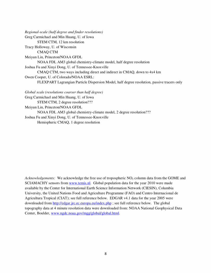
Regional-scale (half degree and finder resolutions)

Greg Carmichael and Min Huang, U. of Iowa

STEM CTM, 12 km resolution

Tracy Holloway, U. of Wisconsin

CMAQ CTM

Meiyun Lin, Princeton/NOAA GFDL

NOAA FDL AM3 global chemistry-climate model, half degree resolution

Joshua Fu and Xinyi Dong, U. of Tennessee-Knoxville

CMAQ CTM, two ways including direct and indirect in CMAQ, down to 4x4 km

Owen Cooper, U. of Colorado/NOAA ESRL:

FLEXPART Lagrangian Particle Dispersion Model, half degree resolution, passive tracers only

Global scale (resolutions coarser than half degree)

Greg Carmichael and Min Huang, U. of Iowa

STEM CTM, 2 degree resolution???

Meiyun Lin, Princeton/NOAA GFDL

NOAA FDL AM3 global chemistry-climate model, 2 degree resolution???

Joshua Fu and Xinyi Dong, U. of Tennessee-Knoxville

Hemispheric CMAQ, 1 degree resolution

Acknowledgements: We acknowledge the free use of tropospheric NO2 column data from the GOME and

SCIAMACHY sensors from www.temis.nl. Global population data for the year 2010 were made

available by the Center for International Earth Science Information Network (CIESIN), Columbia

University, the United Nations Food and Agriculture Programme (FAO) and Centro Internacional de

Agricultura Tropical (CIAT); see full reference below. EDGAR v4.1 data for the year 2005 were

downloaded from http://edgar.jrc.ec.europa.eu/index.php ; see full reference below. The global

topography data at 4 minute resolution data were downloaded from: NOAA National Geophysical Data

Center, Boulder, www.ngdc.noaa.gov/mgg/global/global.html.

9

Table 1. Summary of Work Package 3.2

Work Package 3.2 Title Inflow processes influencing air quality over the

Western North America Lead Owen Cooper Contributor Greg Carmichael, Joshua Fu, Tracey Holloway, Meiyun Lin Start date 01.06.2012 End date 01.05.2014 Objectives:

To evaluate the ability of global and regional models to represent processes driving the import of intercontinental air pollution into western North America and its influence on surface air quality using observations from intensive field campaigns in May-June 2010.

Task Descriptions: Task 3.2.1 Contribute to specifications document of model experiments (WP 2.2)

Identify the model outputs needed to perform the model to observation comparisons needed in Task 3.2.3.

Task 3.2.2 Collect relevant measurement data and make available in networked

archive Identify the available observational data sets for the time and spatial domain of interest: Western North America, for May-June 2010. Make data sets available through one of the distributed archives participating in Theme 6 (AeroCom, NILU, ENSEMBLE, …) or create a new node in the data network. Note that much of the relevant observational data from national networks will already be available through ENSEMBLE for purposes of AQMEII. Relevant observational data include:

• CALNEX, CalMex and CARES field experiments

• Routine surface hourly meteorological observations from NWS

• National Weather Service rawinsondes

• NPS, IMPROVE

• CASTNET • NOAA Trinidad Head surface, ozonesondes, lidar

• NASA Table Mountain ozone lidar

• University of Washington Mt. Bachelor Observations

Task 3.2.3 Conduct analysis of 2010 model simulations in comparison to observations Specific analyses that will be conducted include: 1) Compare model daytime boundary layer depth to temperature and

humidity profiles from the rawinsonde network. Do the models accurately simulate the entrainment of free tropospheric air into the ABL? Comparisons will be made on a monthly basis (May and June), as well as on a daily basis for case studies.

2) Use the rawinsonde network to identify the general structure of the subsidence inversion associated with the eastern North Pacific anticyclone. How do the models simulate this inversion and what effect

10

does it have on the quantity of pollutants entrained into the ABL? How much of the upwind pollution that impacts the receptor region is imported entirely within the ABL and how much descends into the ABL?

3) Compare modeled ozone and PM to the ozonesondes and to the measured values at high and low elevation surface sites across western North America. What is the influence of terrain on the quantity of pollution transported to the surface? Are impacts greatest in the high elevation regions of Nevada, Utah, Arizona and Colorado?

4) Perturbation experiments: What is the impact of 20% reduction and 20% increases in East Asian emissions on ozone and PM in western N. America? Are impacts proportional at both high and low elevation sites? Are impacts proportional in rural and urban areas?

5) When assessing the impacts of foreign pollution at the surface, attention will be paid to the absolute contribution to surface pollution and to the number of exceedances of the U. S. National Ambient Air Quality Standards for ozone and PM (as well as exceedances of air quality standards in the neighboring regions of Canada and Mexico).

6) This model intercomparison will benefit greatly from coordination with MICS-III, a multi-scale model intercomparison to evaluate model strengths and weaknesses regarding air quality prediction and assessments in Asia. MICS-III simulations for spring 2010 will improve our understanding of the Asian pollution events that impact western North America.

7) Finally, the results from this regional-scale model inter-comparison will be compared to coarser scale simulations by global scale models participating in the HTAP model experiments. To what degree do regional-scale models improve our understanding of the impacts of intercontinental transport on surface air quality in the receptor region?

Results of analyses will be circulated via the HTAP wiki for comments by Task Force participants.

Task 3.2.4 Publish paper based on analysis. Deliverables: 3.2.1 Model output specification 1-Sep-2012 3.2.2 Observational data available for model evaluation 1-Jan-2013 3.2.3 Draft analysis results 1-Oct-2013 3.2.4 Submit Publication 1-Jan-2014

11

References:

Boersma, K. F., H. J. Eskes and E. J. Brinksma (2004), Error analysis for tropospheric NO2 retrieval from

space, J. Geophys. Res., 109, D04311, doi:10.1029/2003JD003962.

Center for International Earth Science Information Network (CIESIN), Columbia University; United

Nations Food and Agriculture Programme (FAO); and Centro Internacional de Agricultura

Tropical (CIAT). 2005. Gridded Population of the World: Future Estimates (GPWFE). Palisades,

NY: Socioeconomic Data and Applications Center (SEDAC), Columbia University. Available at

http://sedac.ciesin.columbia.edu/gpw

Cooper, O. R., S. J. Oltmans, B. J. Johnson, J. Brioude, W. Angevine, M. Trainer, D. D. Parrish, T. R.

Ryerson, I. Pollack, P. D. Cullis, M. A. Ives, D. W. Tarasick, J. Al-Saadi, and I. Stajner (2011),

Measurement of western U.S. baseline ozone from the surface to the tropopause and assessment

of downwind impact regions, J. Geophys. Res., 116, D00V03, doi:10.1029/2011JD016095.

Dentener F., T. Keating and H. Akimoto (eds.) Hemispheric Transport of Air Pollution 2010, Part A:

ozone and Particulate Matter, Air Pollution Studies No. 17, United Nations, New York and

Geneva, ISSN 1014-4625, ISBN 978-92-1-117043-6.

Emery et al. (2012), Regional and global modeling estimates of policy relevant background ozone over

the United States, Atmos. Environ., 47, 206-217.

European Commission, Joint Research Centre (JRC)/Netherlands Environmental Agency (PBL).

Emission Database for Global Atmospheric Research (EDGAR), release version 4.1.

http://edgar.jrc.ec.europa.eu, 2010.

Fischer, E. V., K. D. Perry, and D. A. Jaffe (2011a), Optical and chemical properties of aerosols

transported to Mount Bachelor during spring 2010, J. Geophys. Res., 116, D18202,

doi:10.1029/2011JD015932.

Fischer, E. V., D. A. Jaffe, and E. C. Weatherhead (2011b), Free tropospheric peroxyacetyl nitrate (PAN)

and ozone at Mount Bachelor: potential causes of variability and timescale for trend detection,

Atmos. Chem. Phys., 11, 5641-5654.

Huang, M., G. R. Carmichael, B. Adhikary, S. N. Spak, S. Kulkarni, Y. F. Cheng, C. Wei, Y. Tang, D. D.

Parrish, S. J. Oltmans, A. D'Allura, A. Kaduwela, C. Cai, A. J. Weinheimer, M. Wong, R. B.

Pierce, J. A. Al-Saadi, D. G. Streets, and Q. Zhang (2010), Impacts of transported background

ozone on California air quality during the ARCTAS-CARB period – a multi-scale modeling

study, Atmos. Chem. Phys., 10, 6947-6968.

Hudman, R. C., D. J. Jacob, O.R. Cooper, M. J. Evans, C. L. Heald, R. J. Park, F. Fehsenfeld, F. Flocke,

J. Holloway, G. Hübler, K. Kita, M. Koike, Y. Kondo, A. Neuman, J. Nowak, S. Oltmans, D.

Parrish, J. M. Roberts, and T. Ryerson, Ozone production in transpacific Asian pollution plumes

and implications for ozone air quality in California, J. Geophys. Res., 109, D23S10,

doi:10.1029/2004JD004974, 2004.

Lam, Y. F. and J. S. Fu (2010), Corrigendum to "A novel downscaling technique for the linkage of global

and regional air quality modeling", Atmos. Chem. Phys., 10, 4013-4031.

Langford, A. O., J. Brioude, O.R. Cooper, C.J Senff, R.J. Alvarez II, R.M. Hardesty, B.J. Johnson, and

S.J. Oltmans (2012), Stratospheric influence on surface ozone in the Los Angeles area during late

spring and early summer of 2010, J. Geophys. Res., 117, D00V06, doi:10.1029/2011JD016766.

12

Lin, M., Holloway, T., Carmichael, G. R., and Fiore, A. M.: Quantifying pollution inflow and outflow

over East Asia in spring with regional and global models, Atmos. Chem. Phys., 10, 4221-4239,

doi:10.5194/acp-10-4221-2010, 2010.

Lin, M., A. M. Fiore, L. W. Horowitz, O. R. Cooper, V. Naik, J. Holloway, B. J. Johnson, A.

Middlebrook, S. J. Oltmans, I. B. Pollack, T. B. Ryerson, J. X. Warner, C. Wiedinmyer, J.

Wilson, B. Wyman (2012), Transport of Asian ozone pollution into surface air over the western

United States in spring, J. Geophys. Res., in-press.

Wang, Y., Y. Choi, T. Zeng, B. Ridley, N. Blake, D. Blake, and F. Flocke (2006), Late-spring increase of

trans-Pacific pollution transport in the upper troposphere, Geophys. Res. Lett., 33, L01811,

doi:10.1029/2005GL024975.

Zhang, L., D. J. Jacob, N. V. Downey, D. A. Wood, D. B., C. C. Carouge, A. van Donkelaar, D.B.A.

Jones, L. T. Murray, Y. Wang (2011), Improved estimate of the policy-relevant background

ozone in the United States using the GEOS-Chem global model with ½ x 2/3 horizontal

resolution over North America, Atmos. Environ., 45, 6769-6776.

13

Figure 1. Tropospheric NO2 column retrievals from the SCIAMACHY sensor, averaged over April-May

2009-2011. Gridded data used in this plot were freely downloaded from: www.temis.nl

Figure 2. Trends in tropospheric column NO2, as detected by GOME/SCIAMACHY (gridded data used in

these plots were freely downloaded from www.temis.nl), and anthropogenic CO2 emissions (U.S. Energy

Information Agency).

14

Figure 3. The human population of mid-latitude western North America in 2010, and the land-based

anthropogenic NOx emissions in 2005 (EDGAR v4.1). Also shown is the corresponding topography at 7

km resolution, and half degree resolution.

15

Figure 4. Locations of the NWS daily rawinsondes (magenta circles), the May-June 2010 daily

ozonesondes (yellow), and the additional May-June 2010 daily rawinsondes launched from the CARES

sites (white) and the CalMex site (red). NOAA radar wind profilers (not shown) were also situated in the

LA Basin (5 profilers), the Central Valley (5 profilers) and on the coast north of San Francisco (1).

Figure 5. Locations of the CASTNET and National Park Service rural ozone monitors (magenta circles)

and the University of Washington Mt. Bachelor (yellow) and the NOAA Trinidad Head (red) monitors.

16

Figure 6. Map showing the locations of the IMPROVE particulate matter monitoring network.

IMPROVE data are available for download from http://views.cira.colostate.edu/fed/.

Figure 7. a.) Locations of the daily ozonesonde sites in May-June 2010, and the regions of the Central

Valley and the LA Basin sampled by the NOAA P3 aircraft (blue shading). The numbered transects

correspond to the ozone curtains in b. (Transect 1), c. (Transect 2) and d. (Transect 3). The O3 curtains

are median profiles using all available ozonesonde measurements at each site, or all available NOAA P3

measurements above the Central Valley and the LA Basin. Figures are from Cooper et al., 2011.

17

Figure 8. Major trans-Pacific Asian pollution events in May-June 2010 as seen from AIRs retrievals of

CO total columns (1018 molecules cm-2; level 3 daily 1 degree gridded products). Reprint from Lin et al.,

2012.