TART CHERRY YIELD AND ECONOMIC RESPONSE TO ALTERNATIVE PLANTING DENSITIES

By

Nathalie Mongue Me-Nsope

A PLAN B PAPER

Submitted to Michigan State University

in partial fulfillment of the requirements for the degree of

MASTER OF SCIENCE

Agricultural Economics

2009

ABSTRACT

TART CHERRY YIELD AND ECONOMIC RESPONSE TO ALTERNATIVE PLANTING DENSITIES

By

Nathalie Mongue Me-Nsope

The study investigates the economic response of tart cherry yields to planting density

using an unbalanced longitudinal yield data from tart cherry orchards in Northwest

Michigan. The relationship between tart cherry yield and tree age is specified as a linear

spline function and planting density interacts with tree age. A random effect method,

treating block as random, is used to estimate the spline function. Stochastic simulation

was used to estimate the mean and variance of the product of two random variables (price

and yield), and the coefficient of variation was used as a measure of how much risk is

involved in corn/soybeans production relative to tart cherries production. Estimates of the

variance provided the discount factor (10%) and with yields predicted from the statistical

model, relevant cost data and prices, a deterministic simulation was performed to

determine the economically optimal planting density, using annualized net present value

(ANPV) as the decision-making criterion. Results of the study show that at a discount

rate of 10% and tart cherries priced at $0.30 per lb, planting 160 trees per acre is most

profitable. A sensitivity analysis is carried out to determine the effect of variation in

interest rates and tart cherry prices on the optimal planting density. Changing the discount

rate to 12% or 15% or the price to $0.50/lb did not change the most profitable planting

density.

iii

DEDICATION

This work is dedicated to my son, Karsten and

To my nieces: Daniella, Sydney and Chelsey Ekane

for their love and fun in times of stress and desperation.

iv

ACKNOWLEDGMENTS

Special thanks to my research advisor, Dr. Roy Black for his knowledge, time and other

resources put together to see this work accomplished. It would not have been possible

without him. Thanks to other members of my committee: Dr. Scott Swinton for helping

me develop my knowledge base for this topic in the Production Economics class as well

as the very useful comments on the final draft; Dr. Jeffery Andresen for his comments on

the paper and to Dr. John Staatz for his guidance, encouragements and the funds

provided to see this work accomplished. Many thanks to other lecturers:- Dr. Bob Myers

in whose Introductory Econometric class I learnt some basis skills used in this study and

to Dr. Eric Crawford whose Cost Benefit class enhanced my understanding of the

economic model used in this study. Several colleagues also merit mention in their support

of this work: Nicole Olynk, Nicole Mason, Joshua Ariga, Alda Tomo, Malika Chaudhuri,

Tina Plerhoples, Kirimi Sindi, Adjao Ramzi and Mukumbi kudzai.

v

TABLE OF CONTENTS

LIST OF TABLES ………………………………………………………………………v

LIST OF FIGURES …………………………………………………………………….vi

INTRODUCTION ……………………………………………………………………….1

RESEARCH PROBLEM/ KEY RESEARCH GAPS TO EXPLORE……………….......4

RESEARCH OBJECTIVES………………………………………………………...........7

THEORETICAL FRAMEWORK ……………………………………………………….8

METHODS……………….……………………………………………………………...14

DATA AND MODEL…………………………………………………...……………....15 Economic data ……………………………………………………......................15 Economic model ……………………………………………..……………….....17 Tree data………………………………. ……………………….... …………….22 Statistical model for the joint response of tart cherry yields to tree age and planting density……………………………………..........25

RESULTS AND DISCUSSION………………………………………………………..39

SUMMARY OF FINDINGS, CHALLENGES AND RECOMMENDATION ……….49

REFERENCES………………………………………………………………………….53

vi

LIST OF TABLES

Table 1 Estimated Tart Cherry Yield Trajectory (NW Michigan)………………..5

Table 2 Cost Data and Calculations…………………………………..................17

Table 3 Structure of tart cherry tree data under study. ……………………….....24

Table 4 Average yield per acre by tart cherry tree age and number of Blocks measured.…………………… ……………………....................27

Table 5 Blocks meeting statistical Estimation requirements…………………....29

Table 6 Inter-block variation in Yield response to Age………………………32-34

Table 7 Results of the random effect regression of the joint response of Tart cherry yields to tree age and planting density. …………………....40 Table 8 Variation in predicted NPV with Planting Density……………………..46

Table 9 Effect of varying Discount Rate on NPV and ANPV…………………..48

Table 10 Effect of varying Prices on NPV and ANPV…………………………....48

vii

LIST OF FIGURES

Figure 1 U.S., Michigan, and NW Tart Cherry Production (1992-2006)…………1

Figure 2 Michigan Tart Cherry Growing Areas………………………………….2

Figure 3 Estimated Tart Cherry Yield Response to Tree Age…………………….5

Figure 4 Hypothesized pattern of the Tart Cherry yield-age relationship (NW Michigan)………………………………………………………………..9

Figure 5a Effect of Site Quality on Yield-Age Trajectory ……………………….12

Figure 5b Effect of Planting Density on Yield-Age Trajectory…………………..12

Figure 6 Flow chart to illustrate the Method……………………………………15

Figure 7a Residuals Vs Predicted Yields………………………………………...42

Figure 7b Residuals against Tree Age ……………………………………….. ....43

Figure 7c Residuals against Trees per Acre ……………………………………..43

Figure 8 Estimated Joint Response of Tart Cherry to Tree Age and

Planting Density………………………………………………………44

Figure 9 Plot of ANPV @ 10% against Planting Density……………………...47

1

INTRODUCTION

Tart cherry is a perennial tree fruit produced in Michigan, Utah, Washington, New York

and Wisconsin in the United States (U.S.) and widely consumed in different forms

(frozen, fresh, and processed). The U.S. typically produces more than 200 million

pounds of tart cherries each year1 with significant year-to-year variability associated with

weather conditions. In 2002, for example, the crop was severely damaged in Michigan by

a non-inversion frost followed by an inversion frost resulting in zero or near zero yields.

Much of the production is concentrated in Michigan (70-75%) and Northwest (NW)

Michigan grows about 60 percent of Michigan’s total. Figure 1 describes U.S.,

Michigan, and NW Michigan production from 1992-2006 and illustrates the trends and

variability in production.

Figure 1. U.S., Michigan and North West Michigan Cherry Production. (1992-2006)

050

100150200250300350400450

1992

1993

1994

1995

1996

1997

1998

1999

2000

2001

2002

2003

2004

2005

2006

Year

Prod

uctio

n in

mill

ion

poun

ds

NW MichiganTotal - MichiganTotal - U.S.

Source1: Pollack and Perez (2008) Source 2: Cherry Industry Administrative Board (2009)

1 http://www.cherryfestival.org/aboutus/history.php

2

Fluctuations in yield due to spring frost damage is observed to be common and the single

most important weather related risk in Michigan tart cherry industry . However, tart

cherries’ proximity to Lake Michigan which bounds the west side of Michigan gives it a

comparative advantage in tart cherry production (Figure 2). The lake provides a local

warming effect during the night that helps to reduce the likelihood of severe spring

freezes during critical stages of flower bud development. Site choice is an important

determinant of the expected yield (in a probabilistic sense).

Figure 2 Michigan Tart Cherry Growing Areas.

Perennial crop production is distinguished from annual crop production by the long

gestation period, time lag between initial input and first output, an extended period of

output flowing from the initial investment decisions and eventually a gradual

deterioration of the production capacity of the plant (French and Matthews, 1971). Tart

3

cherry production involves farmers making complex design, replacement and annual

management decisions. A common assumption in perennial crop studies is that the

potential profitability of an orchard planting system is the most important factor in the

decision a grower makes when planting a new orchard (Robinson et. al, 2007). Design

decisions include site, acreage, cultivar/variety and planting density (number of trees

planted per acre of land). Replacement is a strategic, longer reaching decision. Finally

tactical management decisions include timing of the harvest, quantity of the fruits to

harvest, pest and disease control and pruning. Pruning and disease control decisions have

both current and future year impacts since they influence the long-run productivity of the

cherry tree.

These decisions or choice of strategy are critical because 1) they involve high costs of

reversal and influence earnings for the next 20 to 30 years and 2) are made in the context

of risk. Risk involved in tart cherries can be described as revenue risk. Revenue risk

could in turn be subdivided into risk associated with variations in tart cherry prices as

well as production risk. This study focuses on production risk, how it affects yields and

how this in turn affects revenues. Production risk is categorized further into trajectory

risk (risk associated to the shape of the tart cherry yield response) as well as the

variability in yield around a trajectory. These two categories of production risk have a

different impact on new investment versus replacement decisions. For instance while the

decision question of making investments in new sites can be treated as a random effect in

a statistical model framework ( since little can be said about the productivity of the site),

replacement decisions can be treated as fixed effects because the productivity of the site

4

is known at the time replacement decision is made. Further explanation on how the

method used depends on the decision questions is provided under the section on

theoretical framework underlying the study and methods.

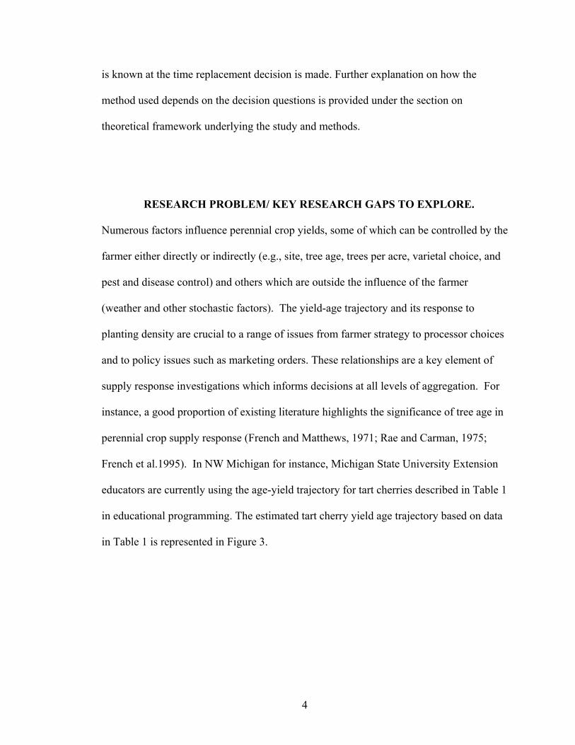
RESEARCH PROBLEM/ KEY RESEARCH GAPS TO EXPLORE.

Numerous factors influence perennial crop yields, some of which can be controlled by the

farmer either directly or indirectly (e.g., site, tree age, trees per acre, varietal choice, and

pest and disease control) and others which are outside the influence of the farmer

(weather and other stochastic factors). The yield-age trajectory and its response to

planting density are crucial to a range of issues from farmer strategy to processor choices

and to policy issues such as marketing orders. These relationships are a key element of

supply response investigations which informs decisions at all levels of aggregation. For

instance, a good proportion of existing literature highlights the significance of tree age in

perennial crop supply response (French and Matthews, 1971; Rae and Carman, 1975;

French et al.1995). In NW Michigan for instance, Michigan State University Extension

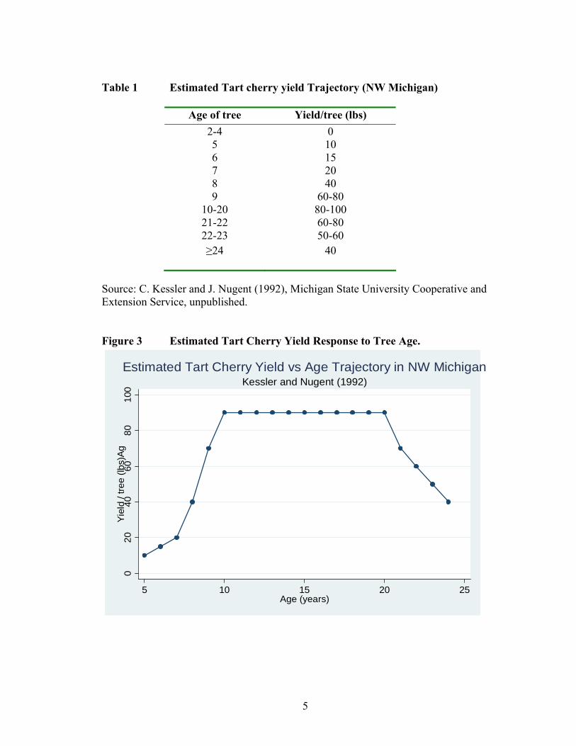
educators are currently using the age-yield trajectory for tart cherries described in Table 1

in educational programming. The estimated tart cherry yield age trajectory based on data

in Table 1 is represented in Figure 3.

5

Table 1 Estimated Tart cherry yield Trajectory (NW Michigan)

Age of tree Yield/tree (lbs) 2-4 0 5 10 6 15 7 20 8 40 9 60-80

10-20 80-100 21-22 60-80 22-23 50-60 ≥24

40

Source: C. Kessler and J. Nugent (1992), Michigan State University Cooperative and Extension Service, unpublished. Figure 3 Estimated Tart Cherry Yield Response to Tree Age.

020

4060

8010

0Y

ield

/ tre

e (lb

s)Ag

5 10 15 20 25Age (years)

Kessler and Nugent (1992)Estimated Tart Cherry Yield vs Age Trajectory in NW Michigan

6

The number of plants in a crop community and the spatial distribution of the plants are

also important determinants of yield. Wade and Douglas (1990) observe that plant

density determines the number of individuals amongst which the limiting resources must

be shared, whilst plant arrangement controls interception of light or retrieval of that

resource. How planting density affects crop yields and how economic value responds to

planting density has received attention from plant scientists, who have done their

investigations using small plot experiments by varying plant density as a treatment

(Springer and Gillen,2007; Seiter et al, 2004; Ngouajio et al , 2006 and Bednarz et

al.,2006).

Through its impact on perennial crop yields, planting density can potentially influence

the profitability of perennial crop production. Some work has been done to investigate the

impact of variation in planting density on crop yields and hence on the profitability of

perennial tree crop production; however, most of these are done on apples using yield

estimates from field trials or replicated research plots. For instance, Robinson et al

(2007), performs an economic comparison of five high density apple planting systems to

determine which is the most economically profitable. The five planting systems were

evaluated in field trials covering a wide range of densities and the yields for each system

were composite averages derived from several replicated research plots.

No work has been done to investigate the impact of variation in planting density on the

profitability of tart cherry production. This study builds on a statistical model to

determine the impact of variation in number of trees per acre on the flow of tart cherry

7

yields and the resulting impact on the profitability of tart cherry production. The study

seeks to identify the appropriate statistical methods/procedures in determining the impact

of variation in planting density on the tart cherry yield age trajectory and most

importantly on the profitability of tart cherry production. Focus group discussions held

by Dr. Black, J. R. (Department of Agricultural, Food and Resource Economics,

Michigan State University) and James Nugent (Northwest Horticultural Research Station)

with tart cherry farmers in NW Michigan established the need to re-evaluate the response

of tart cherry yields to planting density (Black, J.R., personal Communication) . Tart

cherry farmers need to know: 1) what happens to the trajectory of yield per acre as the

planting density changes, 2) how the planting density affects the optimal economic life of

a block and 3) which planting density gives the highest economic return measured by

annualized net present value (ANPV). ANPV is used in contrast to NPV because it takes

into account potential differences in lifespan (unequal rotation periods).

RESEARCH OBJECTIVES.

A systematic search in the literature revealed no studies on the impact of alternative

planting densities on the trajectory of tart cherry yields. This research therefore seeks to

make an important contribution to the existing literature on perennial tree crops by

providing a road map for framing and defining the appropriate tools/statistical methods

for determining the trajectory for perennial tree crop yield response. The study seeks to

investigate how variations in planting density influence the trajectory of yields per acre

over the lifetime of a tart cherry block and the corresponding effects on the profitability

8

of tart cherry production as measured by the annualized net present value. Specific

objectives of the study include:

1. To estimate the joint response of tart cherry yields to tree age and planting density

using unbalanced, longitudinal data from tart cherry blocks under common

management in NW Michigan.

2. To use information from the estimated tart cherry yield response model to

simulate deterministically the impact of variations in planting density on the

trajectory of yields, cash flows and profitability of production as measured by the

ANPV.

3. To conduct sensitivity analyses to evaluate the impact of variations in tart cherry

prices and interest rates on the optimal planting density and orchard economic

life.

4. Make recommendations on the economically profitable planting density.

The results of this study are of interest to tart cherry farmers in NW Michigan and

members of the tart cherry value chain.

THEORETICAL FRAMEWORK.

As mentioned earlier, tart cherry farmers are faced with critical decision-making

questions. These decision questions may include new site, making new investments or

replacements. Planting decisions are examples of investment decisions and they refer to

all the possible options available to the farmer in varying the firm's future productive

capacity through adjustments of tree stock. Given expected future prices and cost

9

considerations, the farmer is assumed to make decisions about the desired age

composition, the number of trees planted in a block and the choice of inputs in order to

maximize present value over the lifetime of his investments. The normal life of a tart

cherry tree is about 30 years. Hence, farmers who plant trees in year t are concerned

about production over the period t + 5 to t + 30.

The hypothesized pattern in tart cherry production in NW Michigan is graphically

illustrated in figure 4. Trees start bearing at about 4 years after planting; yields are low

but increase slowly (stage 1). Stage 2 begins at about 5-6 years after planting when the

yields begin to rise at an increasing rate and reach a peak at about 12 years. Then, starts

stage 3 during which the yields maintain a steady rise to about 20 years. At stage 4, the

last stage, yields gradually decline, as the trees get older.

Figure 4 Hypothesized pattern of tart cherry yield-Age trajectory. NW

Michigan.

5 10 15 20 25

Tree age (years)

6 10 16 21 26 30 Age(year)

Yield (lbs/ acre)

10

Cultivar, weather/climate or planting density could influence this hypothesized pattern.

For instance a fast growing cultivar can start bearing fruits much earlier or severe

damages due to spring frost when the tree is in stage 2 of its lifecycle can cause yields to

decline to levels below stage one or even more. Higher plant densities would peak faster

and give higher yields over a shorter period. Figures 5a and 5b illustrate two alternative

trajectories for the tart cherry yield-age relationship. The trajectory is conditioned by site

and planting density. Figure 5a illustrates possible differences in trajectory due to

differences in site quality. Such a pattern presents enormous statistical estimation

challenges as it involves capturing the differences in slopes as well as in the location of

the knots2 for trajectories A and B. With perfect information on site quality (site index)

the effect of site on the trajectory can be investigated. However, this falls beyond the

scope of this study which is to investigate the joint response of tree age and planting

density on the trajectory of tart cherry yields.

The second factor that conditions the trajectory and therefore exposes the farmer to some

trajectory risk is planting density. It is argued here that planting density influences the

trajectory of yield per acre over the lifetime of the block3 and hence the rotation4 period.

For instance, one hypothesis is that higher plant densities reach peak production sooner

and decline faster. Therefore, an important decision facing tart cherry farmers is the

number of trees to plant per-acre (planting density). The potential effect of planting

2 Knots refers to points on the trajectory of tart cherry yield-age relationship, where there is a significant change in the pattern of tart cherry yield response to age 3 A block is a piece of land on which tart cherries are grown. Trees on a block share common characteristics such as variety, planting pattern, and exposure to weather/climatic conditions. 4 A rotation period is the length of time from site prepartation to removal and subsequent replanting.

11

density on the tart cherry yield age trajectory is shown in figure 5b. A, B, C and D are

alternative planting densities.

The trend in the trajectory could be either stochastic or a deterministic depending on

whether the slope of the trajectory is drawn from some probability distribution that is

unpredictable or predictable. For instance if the slope of the trajectory increases by

some fixed amount on average but in any given planting density the trend deviates from

the average by some unpredictable random amount, then the trajectory is said to exhibit

a stochastic trend. The type of trend exhibited by the trajectory has implications for

statistical modeling, hence the choice of random versus fixed effect. A fixed effect model

is appropriate when it is assumed that the contribution of each block to our yields follows

a deterministic (non-stochastic) trend that is predictable with yield increasing by some

fixed amount over time, thus allowing us to estimate block specific effects. In contrast,

the random effects approach is appropriate when the assumption is that the trajectory of

tart cherry yields follows a stochastic trend.

12

Figure 5a Effect of Site Quality on Yield-Age Trajectory

Figure 5b Effect of Planting Density on Yield-Age Trajectory.

As mentioned earlier, the observed data is longitudinal with multiple measurements of

each individual block over time. There is considerable variation among blocks in the

number of observations. The formulation of our problem should therefore rest on the

5 10 15 20 Age(year)

A

B

Yield (lbs/ acre)

5 10 15 20 Age(year)

Yield (lbs/ acre)

AB

C

D

13

structure of our data (description of data is provided under the section on data) and the

assumptions we make about the probability distribution of multiple measurements in our

data.

While the maintained hypothesis is that there is a piecewise linear relationship between

yield per acre and tree age (Kessler and Nugent, 1992), no information exists either on

the nature of the relationship between yield per acre and number of trees per acre or on

the effect of trees per acre on the tart cherry yield-age trajectory. Thus in addition to the

study contributing to existing literature by identifying the appropriate statistical tools

necessary in modeling the impact of variation in planting density on the trajectory of

yields and hence the profitability of tart cherries, the study also makes a contribution in

the sense that it is the first study on tart cherries (to the best of my knowledge). For other

perennial tree fruits such as apple, it has been argued that higher planting densities results

in higher early yields and higher cumulative yields than lower planting densities

(Robinson et al, 2007).

Generally, tart cherry production begins with costs, followed by annual benefits that

continue over the full life of the trees until they have reached maturity. Variations in

planting density are hypothesized to cause variations in the flow of benefits -by varying

the pattern of yield over time. Variations in planting density also cause costs of

production to vary over time. Goedegebure (1991, 1993) observe that higher planting

density systems have greater investment costs and annual labor costs than low density

systems. Robinson et al (2007) perform an economic comparison of five high density

14

apple systems. They found that differences in establishment costs were largely related to

tree density. In addition to increased orchard establishment costs (for instance cost

incurred in buying trees ), higher planting density might result in increased orchard

maintenance cost in the earlier years and decrease cost in the later years due to shorter

rotation periods. While this dual effect of planting density on revenue and costs is

recognized, this study focuses on assessing the economic consequences of alternative

planting densities taking into account variations in harvest cost and not maintenance cost.

That is, planting density is allowed to affect net returns through its impact on yield per

acre and the corresponding effect of yield on variable harvesting cost and on gross

revenue. Under such considerations, an appropriate economic decision could be to find

the most profitable planting density. That is, given expected future tart cherry prices, the

planting density that maximizes potential tart cherry yields over time subject to cost

constraints.

METHODS

The analysis consists of two major parts. The first part consists of a statistical estimation

of the joint response of tart cherry yields to tree age and planting density and predicting

values for yields over the lifetime of the block. The second part is the economic analysis

and the economic choice criterion employed in the study is ANPV maximization. This

part entails using estimates from the statistical model with relevant price and cost

information to determine the profitability of production for different planting densities as

15

measured by the ANPV. Figure 6 is a flow chart that outlines the major sections of the

methods used in the analysis.

Figure 6 Flow chart to illustrate the method

DATA AND MODEL.

Economic Data

Price data used in this study are “Annual prices received for tart cherries”, obtained from

NASS,USDA-Quick Statistics5. Relevant cost data are from “Cost of Tart Cherry

Production in Michigan” (Black et al, forthcoming). The document contains cost

evaluations, developed through focus group discussions with cherry growers in each of

the production regions in Michigan. The budget includes cash and labor costs per acre for

large -scale cherry growers in the NW Michigan. For the non-bearing years major

components of costs associated with establishing the orchard include; site preparation,

planting, culturing and growing. Planting costs, incurred in year 1 is a function of trees

5 http://www.nass.usda.gov/QuickStats/Create_Federal_All.jsp#top

Annualized Net Present Value (9)

Predicted yields (2)

Gross Revenue (4)

Net cash Flows(6)

Cash Requirements (5)

Estimated Yield (1)

Tart Cherry price (3)

Variance components-measure risk premium (7)

Estimated discount factor (8)

16

planted, so for each of the planting densities considered in the study tree cost ($8.25) was

multiplied by the number of trees planted per acre to obtain planting cost. For years 2, 3

and 4, there is still some variation in cost which causes slight differences in the total cost

estimates for each of these years. Although the activity type is same for years 2, 3 and 4,

the intensity of each activity varies, thus causing cost to vary. For instance pruning takes

place in years 2, 3 and 4. However, in year 2, two hours of pruning, valued at $15.9 per

acre is required, as opposed to three hours per acre ($47.9) and four hours per acre

($63.6) required for years 3 and 4 respectively. Other activities that vary in intensity and

hence cost across years 2, 3 and 4 are mowing, pest control, and management and

fertilizer material. See Table 2 for a breakdown of cost for the non-bearing years.

For the bearing ages, costs for each age beginning at 5 were calculated taking into

account the fact that harvesting begins in year five. As previously mentioned, only

variable components of the harvest cost were allowed to change with planting density.

The following equation was used to calculate the cost for the bearing years:

312 and ,0060.0where

)1..(acre/yield)005.00055.00120.0(acre/yield).acre/yield

(acre/cost

10

10

==

×+++×+=

γγ

γγ

The parameters in the cost equation were established from a budget system developed by

J.R Black and J. Nugent in a focus group discussion with tart cherry growers in each of

the production regions in Michigan. The parameter 0γ was fixed irrespective of the rate

of production while 1 γ depended on the rate of production. The cost equation was

17

constructed to reflect decreasing cost per pound. Harvest costs had both fixed

(equipments) and variable components. Fix components include; cost of 80 HP

tractor/forklift, 85 HP tractor/forklift, double incliner shaker and skimmer. The variable

costs that entered the calculations include; a) shipping charged at 0.0120 cent/pound, b)

cooling pad operation charged at 0.00550 cents/pound and Tart Cherry Assessment6 cost

charged at 0.00500 cent/pound, which are multiplied by yield per acre in equation 1.

Table 2 Cost Data and Calculations.

Age Activity Cost ($) per Acre

0 Site Preparation and Fallow 900

1 Planting and Culturing 754+ (trees per acre) x $8.25

2 Growing 319

3 Growing 361

4 Growing 378

5 Growing+ other Operations, 456+ cost calculated using equation 1

6-25 Operations, harvest and

management

Cost calculated using equation 1

Adapted from Black et al, forthcoming.

The Economic Model.

The objective of the economic model is to determine the planting density that maximizes

ANPV. The economic model describes the costs and revenues associated with fruit

6 Assessment for advertising/ promotion of product.

18

production in an orchard system from planting to maturity. Predicted annual tart cherry

yields from the statistical model and exogenously given prices are used to calculate the

annual revenue from the system. The prices used in calculating the gross revenue are

market prices averaged over a period of time. In principle, gross revenue should be yield

multiplied by the effective price, which is the market price adjusted for quality (which is

in turn a function of the age of the block). However, because of lack of data on fruit

quality, the prices used in the analysis were not adjusted to reflect quality. The costs of

establishing the orchard system as well as costs related to tree density and harvest enter

the net cash flow calculation. Apart from the three harvesting costs listed above that

were a function of yields per acre, all other costs were held constant across planting

density.

To determine the profitability of tart cherry production under a specific planting density,

the net cash flows are calculated using equation 27 . Net cash flow in year t is given by

)2(........................................1

)0(∑=

+−=i itCtCtytPtNCF

where NCFt is the net cash flow at time period t, Pt is the average market price for tart

cherry calculated from historical price data of tart cherry, yt is tart cherry yield for a

given tree age and planting density combination. Multiplying average prices and yield for

a given age and planting density generates a stream of revenue over time. The cost of

establishing the orchard system from bare ground (Cot) as well as costs related to tree

density and harvest, Cit enters the net cash flow calculations.

7 Equations 2, 3 and 4 are adapted from AEC 865 “Agricultural Cost Benefit Analysis” lecture notes.

19

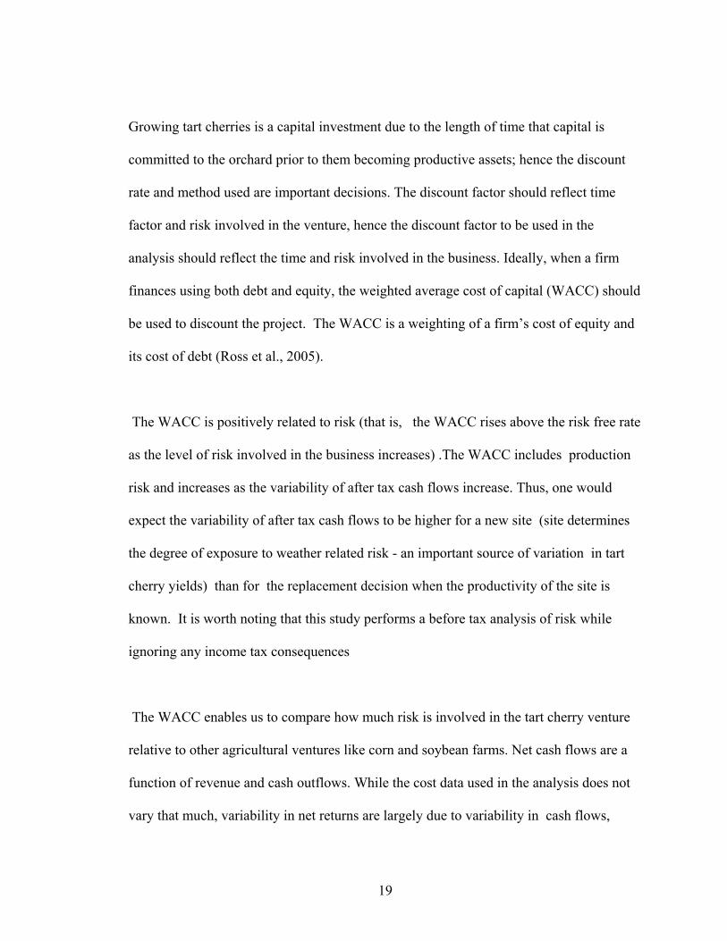
Growing tart cherries is a capital investment due to the length of time that capital is

committed to the orchard prior to them becoming productive assets; hence the discount

rate and method used are important decisions. The discount factor should reflect time

factor and risk involved in the venture, hence the discount factor to be used in the

analysis should reflect the time and risk involved in the business. Ideally, when a firm

finances using both debt and equity, the weighted average cost of capital (WACC) should

be used to discount the project. The WACC is a weighting of a firm’s cost of equity and

its cost of debt (Ross et al., 2005).

The WACC is positively related to risk (that is, the WACC rises above the risk free rate

as the level of risk involved in the business increases) .The WACC includes production

risk and increases as the variability of after tax cash flows increase. Thus, one would

expect the variability of after tax cash flows to be higher for a new site (site determines

the degree of exposure to weather related risk - an important source of variation in tart

cherry yields) than for the replacement decision when the productivity of the site is

known. It is worth noting that this study performs a before tax analysis of risk while

ignoring any income tax consequences

The WACC enables us to compare how much risk is involved in the tart cherry venture

relative to other agricultural ventures like corn and soybean farms. Net cash flows are a

function of revenue and cash outflows. While the cost data used in the analysis does not

vary that much, variability in net returns are largely due to variability in cash flows,

20

which are in turn triggered by variability in yield and tart cherry prices. Yield variability

is measured by variance from our statistical model.

Given that cash flows from a tart cherry crop cycle extend over several years, any

analysis of that cash flow should incorporate the time value of money. The Net Present

Value (NPV) for a given mean planting density is calculated by discounting the net cash

flows over time (revenue net of expenses for each year) summed over the lifetime of the

investment) at the farm’s opportunity cost of capital.. The net present value of the stream

of annual profits obtained over the planning horizon t=1,…,T is defined as:

[ ] ....(3)........................................

1 1NPV ∑

= +=

T

t ttNCF

α

where: NCF = annual net cash flows in period t (cash inflows minus cash outflows), t = annual index, α = the discount rate, T = the length of the investment.

When comparing investments of different lengths, it is desirable to compare them in

annuity form. To compare the relative profitability of different planting densities the net

present value of the income stream must be annualized or converted to an average net

return per year. This annualized value is obtained using:

ANPV = NPV x [r / 1 - (1 + r) -n]………………………………(4)

Where r is the economic discount rate and n is the length of the rotation period.

21

The annualized net present value (ANPV) for a given planting density income stream

can be interpreted as the average net return per acre per year over a particular planting

density adjusted for the time value of money.

Annual yields are recalculated for different planting densities chosen arbitrarily and the

economic model is simulated to determine the impact of variation in average planting

density on annual tart cherry yields and consequently on the annualized net present value

of the income stream. Such a deterministic simulation model is particularly useful means

to evaluate the effects on yield and profitability of alternative planting density and other

decisions under the direct control of the grower. The optimal planting density maximizes

the ANPV of the income stream. If a planting density results in a decrease in the average

annualized net income, it should not be considered even if a profit can be made from its

harvest.

The length of the time horizon, T, also influences system ANPV. The time horizon is

important in assessing orchard rotation strategies. Furthermore, an objective of this study

is to determine the optimal economic life of the orchard block. That is, what is the

marginal net revenue derived as a result of holding the block for an additional year? The

optimal economic life is driven by fruit quality (as well as yields) and may vary with

number of trees planted per acre. Discussions with some farmers from Northwest

Michigan revealed that fruit quality is dropping off in instances where the blocks were

being pulled. With no data on fruit quality, the effect of fruit quality on the optimal

economic life cannot be determined. Moreover, different planting densities are

22

hypothesized to result to different rotation periods, which ideally should be reflected in

the computation of the ANPV, but data series was not long enough to test for this.

Tree Data.

The study uses a longitudinal dataset from a single farm with multiple tart cherry

producing blocks, producing the Montmorency variety, under common management and

located in Northwest Michigan. For confidentiality reasons, additional information on the

tart cherry farm used for this study cannot be disclosed. Not all blocks were started under

the same management. Some were started under the current management while others

were acquired from other farmers. The planting density differs across blocks but is

constant over time within a block. The blocks are spatially diversified resulting in

variation in weather exposure and site quality. The blocks vary in year planted and

therefore age and are measured at regular intervals (annually) over a period for yields.

The oldest measurements for tart cherry yields were taken in 1979 and the youngest in

2003. Tree yields vary with age within a given block and across blocks measured at

similar ages.

The number of measurement occasions varies across blocks thus resulting in variation in

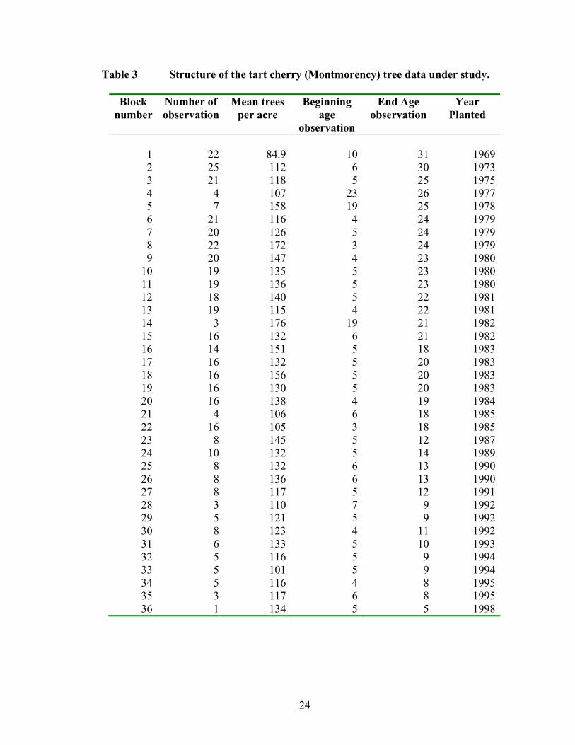
number of observation across blocks; hence we have an unbalanced data. See Table 3 for

a general description of the dataset. Block number is just a number assigned by the

researcher to identify each block. Trees per acre are the number of trees planted per acre.

Beginning age observation is the age of the trees when the tree was first measured for

23

yields. End age observation is tree age at last measurement and year planted is the year in

which the block was planted. An examination of the age variable in the data reveals

possibility of selection bias; very few blocks of trees are older than 25 years. The trees

might have been pulled out because of the quality of the fruits. Data also contains

information on number of acres per block, tree yields by block, and total production.

24

Table 3 Structure of the tart cherry (Montmorency) tree data under study.

Block number

Number of observation

Mean trees per acre

Beginning age

observation

End Age observation

Year Planted

1 22 84.9 10 31 19692 25 112 6 30 19733 21 118 5 25 19754 4 107 23 26 19775 7 158 19 25 19786 21 116 4 24 19797 20 126 5 24 19798 22 172 3 24 19799 20 147 4 23 1980

10 19 135 5 23 198011 19 136 5 23 198012 18 140 5 22 198113 19 115 4 22 198114 3 176 19 21 198215 16 132 6 21 198216 14 151 5 18 198317 16 132 5 20 198318 16 156 5 20 198319 16 130 5 20 198320 16 138 4 19 198421 4 106 6 18 198522 16 105 3 18 198523 8 145 5 12 198724 10 132 5 14 198925 8 132 6 13 199026 8 136 6 13 199027 8 117 5 12 199128 3 110 7 9 199229 5 121 5 9 199230 8 123 4 11 199231 6 133 5 10 199332 5 116 5 9 199433 5 101 5 9 199434 5 116 4 8 199535 3 117 6 8 199536 1 134 5 5 1998

25

Statistical Model for the joint response of tart cherry yields to tree age and planting

density.

The purpose of statistical model is to obtain statistical parameters/estimates that

capture/describe the relationship between tart cherry yields, tree age and planting density.

Two important issues are dealt with in this subsection: a) choosing a functional form that

captures the nature of the relationship between tart cherry yields and tree age and planting

density, and b) sampling and error structure. The choice of the functional form is driven

by the underlying notion that perennial crop yields vary with variation in the age of the

tree. From our hypothesized tart cherry yield age relationship, four different linear

relationships exist between tree age and tart cherry yields for each stage of the lifecycle.

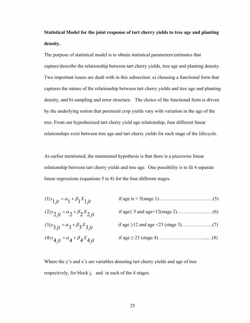
As earlier mentioned, the maintained hypothesis is that there is a piecewise linear

relationship between tart cherry yields and tree age. One possibility is to fit 4 separate

linear regressions (equations 5 to 8) for the four different stages.

jtjt Xy 1111)1( βα += if age is < 5(stage 1)……………………………(5)

jtjt Xy 2222)2( βα += if age≥ 5 and age<12(stage 2)………………….(6)

jtjt Xy 3333)3( βα += if age ≥12 and age <23 (stage 3)……………….(7)

jtjt Xy 4444)4( βα += if age ≥ 23 (stage 4)………………………........(8)

Where the y’s and x’s are variables denoting tart cherry yields and age of tree

respectively, for block j, and in each of the 4 stages.

26

However, fitting separate linear models for the 4 different stages of the hypothesized

lifecycle will lead to a discontinuous function. We therefore need a mathematical

function that enforces continuity between the stages in our hypothesized yield-age

relationship described above. The model is therefore specified as a linear spline function

that allows us to generate a piecewise continuous yield- age response, resulting in a

smooth curve (Green, 2007). Generally, we do not expect much output within the first

few years after planting because the fruit seeds planted have to grow into trees before

they begin bearing any considerable amount of fruits. Although our data contains some

yields for this stage, we ignore this stage in our analysis. Yield/acre for tree age less than

5 are significantly less than 5000 pounds per acre. Table 4 illustrates a breakdown of

yield per acre by tree age.

27

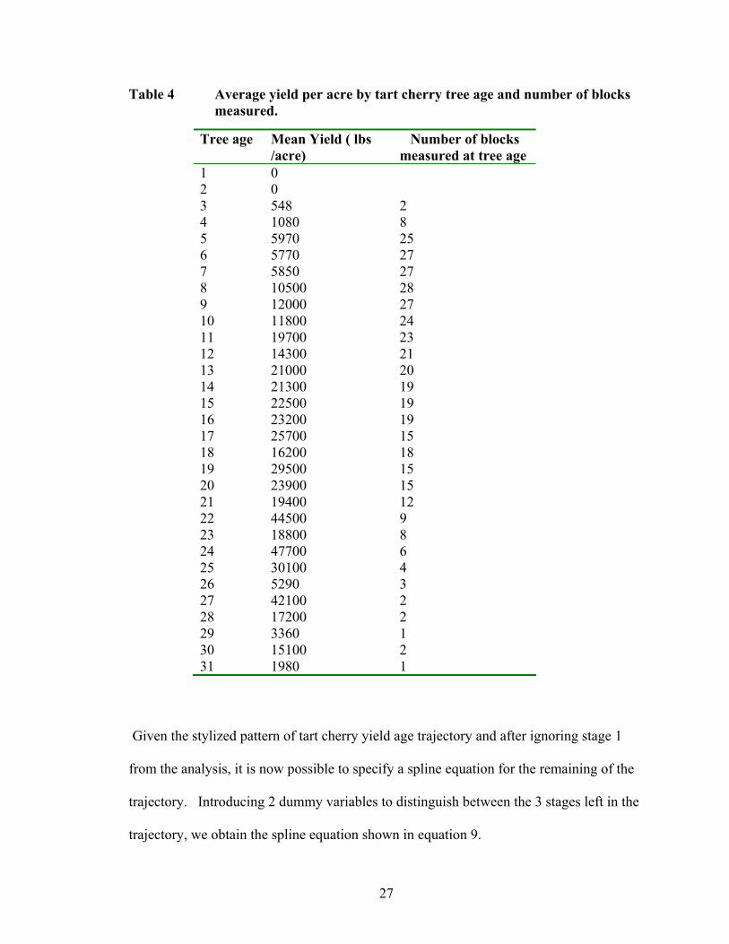
Table 4 Average yield per acre by tart cherry tree age and number of blocks measured.

Given the stylized pattern of tart cherry yield age trajectory and after ignoring stage 1

from the analysis, it is now possible to specify a spline equation for the remaining of the

trajectory. Introducing 2 dummy variables to distinguish between the 3 stages left in the

trajectory, we obtain the spline equation shown in equation 9.

Tree age Mean Yield ( lbs /acre)

Number of blocks measured at tree age

1 0 2 0 3 548 2 4 1080 8 5 5970 25 6 5770 27 7 5850 27 8 10500 28 9 12000 27 10 11800 24 11 19700 23 12 14300 21 13 21000 20 14 21300 19 15 22500 19 16 23200 19 17 25700 15 18 16200 18 19 29500 15 20 23900 15 21 19400 12 22 44500 9 23 18800 8 24 47700 6 25 30100 4 26 5290 3 27 42100 2 28 17200 2 29 3360 1 30 15100 2 31 1980 1

28

(9)----------- )*23(22)*

12(1110 jttjtXdtjtXdjtXjty εβββα +−+−++=

Where d1 and d2 are dummy variables. d1 takes on 1 if in stage 3 and 0 otherwise, and d2

is takes on value 1 if in stage 4 and 0 otherwise. *1t and *

2t are the hypothesized

locations of the knots on the trajectory. In the case of tart cherry for instance, a knot is the

point on the tart cherry yield-age trajectory where there is a remarkable change in the

pattern of the relationship between tree age and tart cherry yields. It is the point that

connects stage 2 to stage 3 and stage 3 to 4.

As shown in table 3, there are few observations with age above 25, this may be a

selection bias issue because the trees were already pulled out. This therefore limits how

much information we have to capture the trajectory in stage 4. Henceforth we limit our

analysis to cases where age is greater than or equal to 5 and less than or equal to 25 years,

thus enabling us to capture stages 2 and 3 of the hypothesized tart cherry yield age

trajectory.

Furthermore, to reduce the effects of the incompleteness of the data, we eliminate blocks

with less than 7 observations. Year 2002 was also dropped from the data because it was a

really bad year thus resulting in extreme values for yields. Table 5 summarizes the

resultant dataset.

29

Table 5 Blocks meeting statistical Estimation requirements.

Block number

Number of observation

Mean trees per acre

Beginning Age observation

End age observation

Year Planted

1 16 84.9 10 31 19692 20 112 6 30 19733 21 118 5 25 19756 19 116 4 24 19797 19 125 5 24 19798 19 172 3 24 19799 18 147 4 23 1980

10 18 135 5 23 198011 18 136 5 23 198012 17 140 5 22 198113 17 115 4 22 198115 15 132 6 21 198216 14 151 5 18 198317 15 132 5 20 198318 15 156 5 20 198319 15 130 5 20 198320 14 138 4 19 198422 13 105 3 18 198523 8 145 5 12 198724 9 132 5 14 198925 7 132 6 13 199026 7 136 6 13 199027 7 117 5 12 1991

The method used in estimating a spline function depends on whether or not the location

of the knot is known with certainty. Generally, when the exact locations of the knots are

known, dummy variables are introduced to distinguish between the different sections of

the curve. However when the location of the knots is not known we use nonlinear least

squares regression to estimate the location of the knots. In our case, the hypothesized

location of the age that separates stage 2 from stage 3 was age=12. Even though non

linear least squares gave tree age 13 as a likely location for the knot with a standard error

of approximately 1.0, graphical examination of the data revealed that age 12 was most

30

logical within 1 standard deviation. Hence we stick with age 12 as knot location between

stage 2 and stage 3.

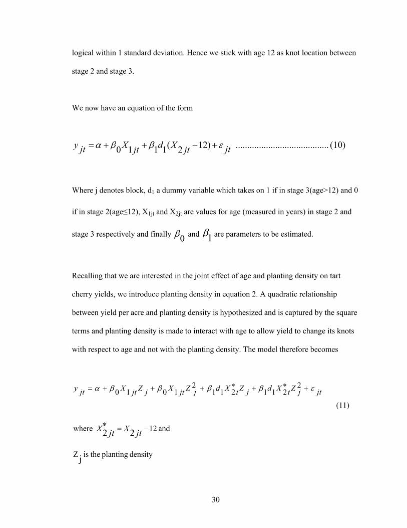
We now have an equation of the form

(10)........................................ )122(1110 jtjtXdjtXjty εββα +−++=

Where j denotes block, d1 a dummy variable which takes on 1 if in stage 3(age>12) and 0

if in stage 2(age≤12), X1jt and X2jt are values for age (measured in years) in stage 2 and

stage 3 respectively and finally 0β and 1β are parameters to be estimated.

Recalling that we are interested in the joint effect of age and planting density on tart

cherry yields, we introduce planting density in equation 2. A quadratic relationship

between yield per acre and planting density is hypothesized and is captured by the square

terms and planting density is made to interact with age to allow yield to change its knots

with respect to age and not with the planting density. The model therefore becomes

(11)

2211211

21010 jtjZtXdjZtXdjZjtXjZjtXjty εββββα +∗+∗+++=

and 12 where 22 −=∗jtjt XX

density planting theis Z j

31

With a functional form for our model, the next issue to be addressed is what estimation

method to use for our model. The formulation of our problem or the choice of method

should be driven by the structure of our data and the assumptions we make about the

probability distributions of the multiple measurements in our data.

Examining the data set reveals variation in crop yields between blocks (even when the

blocks are of the same age- block effect) and variation across time (age effect). The block

effect that implies that yields are random across blocks is investigated by running

separate linear regressions for each block. The results in Table 5 illustrate much

randomness in the slope and intercept coefficients across blocks. Three different

estimations were performed for blocks with at least 7 observations with complete data set

(5≤age≤25), pre-peak data (5≤age≤12), and post-peak data (12<age≤25), respectively to

understand variation in yields across blocks. Peak age is 12.

Table 6 Interblock variations in Yield response to tree age for pre-peak, post peak and complete data. Complete Estimates (5<=Age<=25) Y=β0+β1*Age+β2*d*Age

Pre Peak Estimation 5<=age<=12) Y=β0+β1*Age

Post Peak Estimation (12<age<=25) Y=β0+β1*Age

Block no

No. of observation

β0 β1 β2 Block no.

No. of Observ- ations

β0 β1 Block no.

No. of Observ ations

β0 β1

1 16 -17.4 (15.3)

1.80 (1.33)

1.35

-1.68 (1.4) 1.19

2 7 -5.04 (1.00)

0.80 (0.11)

7.39

1 13 5.85 (3.44)

-0.03 (0.18) -0.16

2 20 -5.10 (2.32)

0.81 (0.23)

3.52

-0.55 (0.29) -1.86

3 8 -6.57 (1.40)

1.20 (0.16)

7.52

2 13 1.52 (2.73)

0.26 (0.14)

1.823 21 -5.06

(2.51) 0.98

(0.26) 3.82

-0.86 (0.35) -2.48

6 8 0.81 (1.29)

0.20 (0.15)

1.37

3 13 3.15 (3.60)

0.22 (0.19)

1.196 19 -0.49

(2.20) 0.39

(0.23) 1.70

-0.19 (0.32) -0.59

7 8 2.56 (1.76)

0.03 (0.20)

0.16

5 7 8.14 (14.02)

-0.15 (0.63) -0.24

7 19 0.21 (2.36)

0.37 (0.24)

1.51

-0.20 (0.35) -0.57

8 8 0.06 (1.76)

0.36 (0.20)

1.82

6 12 7.00 (4.24)

-0.10 (0.23) -0.46

8 19 -1.78 (1.96)

0.63 (0.20)

3.08

-0.49 (0.29) -1.69

9 8 -4.17 (1.97)

0.81 (0.22)

2.61

7 12 9.53 (4.04)

-0.22 (0.21) -1.01

9 18 -5.32 (3.31)

0.97 (0.34)

2.81

-0.91 (0.59) -1.79

10 8 -4.64 (2.47)

0.93 (0.28)

3.31

8 12 10.60 (3.87)

-0.23 (0.21) -1.14

10 18 -6.27 (3.15)

1.16 (0.33)

3.53

-1.16 (0.48) -2.39

11 8 -3.39 (1.80)

0.68 (0.20)

3.31

9 11 11.60 (6.65)

-0.30 (0.36) -0.82

Standard errors are in parenthesis below coefficients and t-values are highlighted

32

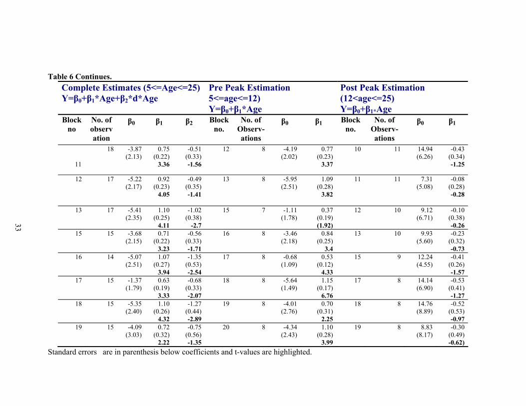
Table 6 Continues. Complete Estimates (5<=Age<=25) Y=β0+β1*Age+β2*d*Age

Pre Peak Estimation 5<=age<=12) Y=β0+β1*Age

Post Peak Estimation (12<age<=25) Y=β0+β1*Age

Block no

No. of observation

β0 β1 β2 Block no.

No. of Observ-ations

β0 β1 Block no.

No. of Observ- ations

β0 β1

11

18 -3.87 (2.13)

0.75 (0.22)

3.36

-0.51 (0.33) -1.56

12 8 -4.19 (2.02)

0.77 (0.23)

3.37

10 11 14.94 (6.26)

-0.43 (0.34) -1.25

12 17 -5.22 (2.17)

0.92 (0.23)

4.05

-0.49 (0.35) -1.41

13 8 -5.95 (2.51)

1.09 (0.28)

3.82

11 11 7.31 (5.08)

-0.08 (0.28) -0.28

13 17 -5.41 (2.35)

1.10 (0.25)

4.11

-1.02 (0.38)

-2.7

15 7 -1.11 (1.78)

0.37 (0.19) (1.92)

12 10 9.12 (6.71)

-0.10 (0.38) -0.26

15 15 -3.68 (2.15)

0.71 (0.22)

3.23

-0.56 (0.33) -1.71

16 8 -3.46 (2.18)

0.84 (0.25)

3.4

13 10 9.93 (5.60)

-0.23 (0.32) -0.73

16 14 -5.07 (2.51)

1.07 (0.27)

3.94

-1.35 (0.53) -2.54

17 8 -0.68 (1.09)

0.53 (0.12)

4.33

15 9 12.24 (4.55)

-0.41 (0.26) -1.57

17 15 -1.37 (1.79)

0.63 (0.19)

3.33

-0.68 (0.33) -2.07

18 8 -5.64 (1.49)

1.15 (0.17)

6.76

17 8 14.14 (6.90)

-0.53 (0.41) -1.27

18 15 -5.35 (2.40)

1.10 (0.26)

4.32

-1.27 (0.44) -2.89

19 8 -4.01 (2.76)

0.70 (0.31)

2.25

18 8 14.76 (8.89)

-0.52 (0.53) -0.97

19 15 -4.09 (3.03)

0.72 (0.32)

2.22

-0.75 (0.56) -1.35

20 8 -4.34 (2.43)

1.10 (0.28)

3.99

19 8 8.83 (8.17)

-0.30 (0.49) -0.62)

Standard errors are in parenthesis below coefficients and t-values are highlighted.

33

Table 6 Continues.

Complete Estimates (5<=Age<=25) Y=β0+β1*Age+β2*d*Age

Pre Peak Estimation 5<=age<=12) Y=β0+β1*Age

Post Peak Estimation (12<age<=25) Y=β0+β1*Age

Block no

No. of observ-ation

β0 β1 β2 Block no.

No. of Observ- ations

β0 β1 Block no.

No. of Observ- ations

β0 β1

20 14 -3.50 (3.30)

0.98 (0.35)

2.78

-1.20 (0.66) -1.82

22 8 -4.29 (1.84)

0.89 (0.21)

4.28

20 7 14.42 (13.16)

-0.51 (0.82) -0.63

22 13 -4.28 (2.27)

0.89(0.25)

3.63

-1.28(0.50) -2.55

23 8 -2.22(2.05)

0.71(0.23)

3.0623 8 -2.22

(2.05) 0.71

(0.23) 3.06

0.00(0.00)

-

24 8 1.60(4.15)

0.44(0.47)

0.94

24

8 -1.94 (3.99)

0.78(0.44)

1.78

-2.59(1.78) -1.46

25 7 5.30(6.57)

-0.08(0.71) -0.12

25 7 -1.30 (6.27)

0.78(0.72)

1.08

0.40(4.61)

0.09

26 7 1.35(5.34)

0.24(0.58)

0.4126 7 -5.11

(3.85) 1.08

(0.44) 2.43

-2.10(2.83) -0.74

27 8 3.17(4.12)

0.19(0.47)

0.4127 7 0.41

(2.64) 0.62

(0.31) 1.99

0.00(0.00)

(-)

30 7 1.83(3.17)

0.13(0.38)

0.34Standard errors are in parenthesis below coefficients and t-values are highlighted.

34

35

Possible causes of variation in tart cherry yield response across blocks could be site. The

site at which a block is located determines degree of exposure to weather/climatic

conditions such as freezes (wind freeze, inversion) and drought, and the extent of

pollination.

An important characteristic of longitudinal data is within and between subject

correlations. Using ordinary, least squares (OLS) methods to estimate this model by

pooling the data would mean ignoring any within-block and between-block correlations.

In the presence of such correlations, OLS could result in inefficient estimates (although

could be consistent in large samples as estimates approach the unknown parameter

value). Examples of models that are capable of handling the unobserved block-specific

effect are the random and fixed effect models.

The fixed effects model is an appropriate specification if we are focusing on a specific set

of N blocks, such that the inference is conditional on the set of blocks that are observed.

A fixed effect model assumes the contribution of each block to our yields follows a

deterministic (non-stochastic) trend that is predictable and it increases by some fixed

amount over time. Thus a fixed effect model allows us to estimate block specific effects.

In contrast, the random effects model is an appropriate specification if we are drawing

many blocks randomly from a large population. With the random effect approach, we

assume that the trajectory of tart cherry yields follows a stochastic trend with the slope

drawn from some probability distribution, which is unpredictable. A stochastic trend

would imply that tart cherry yields increase by some fixed amount on average but in any

36

given block the trend deviates from the average by some unpredictable random amount

that can be modeled using a random effect model.

Thus, viewing blocks as random samples from a population of blocks and assuming

that the probability distribution of the multiple measurements has the same form for each

individual block, but that the parameters of that distribution varies over blocks, a random

effect model is appropriate to estimate the joint response of tart cherry yields to age

and planting density. A random effects model would explicitly account for the

heterogeneity of blocks studied through a statistical parameter representing the inter-

block variation and it allows us to characterize the probability distributions (pattern) for

individual responses and change over time and to investigate the effects of covariates on

these patterns.

The use of a random effects model enables us to draw statistical inferences from

comparable but heterogeneous blocks beyond the particular values used in the study.

Therefore, conceptualizing the selected blocks in the data as pieces randomly drawn from

a larger universe of possible blocks, inferences can be made to a larger universe of

blocks, farm and even location.

Random effect model specification:

Consider the following model;

(12) ...... ....2211211

21010 jtjtjtjtjjt ZXdZXdZXZXjty εββββα +++++= ∗∗

37

This specifies tart cherry yields as a joint function of age and planting density with some

error. jty is the response of block j at time t, X and Z same as above and jtε is the

residual. The residual captures variations in yields due to factors other than tree age and

planting density, some of which can be treated as random across blocks (such as site). To

account for within block dependence, the jtε is split into two components jt∈ and

jtδ which account for deviation of jty from block j’s mean (e.g. due to pest and

disease) and random deviation of block j’s mean yield from the overall mean (site is

treated as random) respectively.

..(13)........... 2211211

21010 jtjtjZtXdjZtXdjZjtXjZjtXjty ∈++∗+∗+++= δββββα

Where jδ ),0( 2τN≈ and ),0( 2jtjt N σ≈∈ .

This is our estimation model.

In addition to the sampling error associated with each block, an assumption behind the

random effects model is that the true yield effect in each time period is influenced by

several factors, including tree characteristics (such as the age of the tree) , planting

density and weather/climatic conditions for that year. The model stipulates that the true

yield effects is given by all terms on the right hand side of equation 13 except jt∈

Where α is the overall yield effect or average yields generated from a population of

possible realizations of yields and jtδ is the deviation of the j-th block’s effect fromα .

38

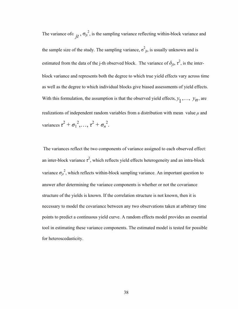
The variance of jt∈ , σjt2, is the sampling variance reflecting within-block variance and

the sample size of the study. The sampling variance, σ2jt, is usually unknown and is

estimated from the data of the j-th observed block. The variance of δjt, τ2, is the inter-

block variance and represents both the degree to which true yield effects vary across time

as well as the degree to which individual blocks give biased assessments of yield effects.

With this formulation, the assumption is that the observed yield effects, 1y ,…, ny , are

realizations of independent random variables from a distribution with mean value μ and

variances τ2 + σ12,…, τ2 + σn

2.

The variances reflect the two components of variance assigned to each observed effect:

an inter-block variance τ2, which reflects yield effects heterogeneity and an intra-block

variance σjt2, which reflects within-block sampling variance. An important question to

answer after determining the variance components is whether or not the covariance

structure of the yields is known. If the correlation structure is not known, then it is

necessary to model the covariance between any two observations taken at arbitrary time

points to predict a continuous yield curve. A random effects model provides an essential

tool in estimating these variance components. The estimated model is tested for possible

for heteroscedasticity.

39

RESULTS AND DISCUSSION

Random effect estimation was carried out on model (13). Results of the estimation are

shown in table 6. Results reveals that while the linear (x1z) and quadratic (x1z2)

interaction between tree age and planting density when tree age is between 5 and 12

inclusive are significant at the 5 percent level, only the linear interaction (dx2z) between

tree age and planting density when tree age is greater than 12 and less than 25 was

significant. The quadratic interaction (dx2z2) in this stage is insignificant at the 5 percent

level. Regression results also show a between blocks (sigma_u in table 7) and within

blocks (sigma_e in table 7) standard deviations of 0.53 and 2.05, respectively. That is, the

between and within block variance is 0.28 and 4.20 respectively. There is much more

variation in yield response within blocks than between blocks. As mentioned earlier,

variation in tart cherry yield age trajectory could be caused by differences in planting

density and/or site quality. Summary of the data used in this analysis (Table 5) supports

some variation in planting density. Weather and pollination are large effects on yield.

Offhand, it should not be surprising that the within block variance is larger than the

between block variance because the within variance captures weather effects. A

maintained hypothesis is that the within variance for poor sites is larger than that for

excellent sites (quality of air drainage). However, we do not have enough information to

test this. The proportion of the total variance in yields contributed by block level variance

in yield response (rho in table 7) is 0.062 (6%).

40

Table 7 Results of the random effect regression of the joint response of tart cherry yields to tree age and planting density

Random-effects GLS

regression Number of observation:295

Group variable: block no Number of groups :18 2R : within:0.5192

2R between: 0.0188

2R overall: 0.4874

Observation per group: minimum:7

average:16.4 maximum:21

Random effects u_i ~ Gaussian

Wald chi2(4) : 292.47

corr(u_i, X) : 0 (assumed)

Prob > chi2 : 0.0000

Yield/acre Coefficient Standard error

z P>|z|

x1z 0095166 0.0014681 6.48 0.000

x1z2 -0.0000264 9.12e-06 -2.89 0.004

dx

2z -0.0060399 0.0029646 -2.04 0.042

dx

2z2 7.12e-06 0000207 0.34 0.732

_cons -3.540716 6263516 -5.65 0.000

sigma_u :0.52985059

sigma_e :2.0528581 Rho : 0.06245687 (fraction of variance due to u_i)

where:

yld_acre denotes yields in tons per acre.

x1z denotes age x tree if age<= 12 years

x1z2 denotes age x planting density squared if age<= 12 years

dx2z denotes age x tree if age> 12 years <25 and

dx1z2 denotes age x planting density squared if age> 12< 25 years

The test for the statistical significance of regression coefficients reveal that while dx2z

and dx2z2 are not both individually significant, they are jointly significant with chi2 ( 2)

41

equals 292.47 and probability greater than chi2 equals 0.00, which may be a result of

multicollinearity amongst these two variables.

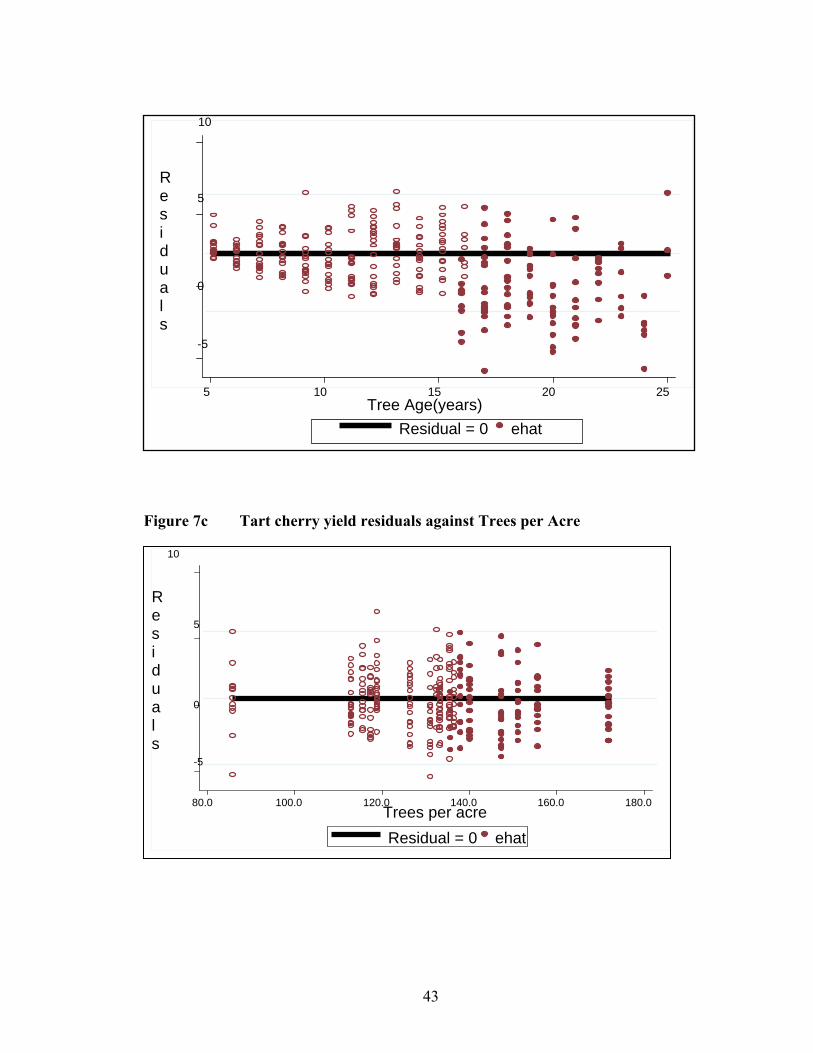
The estimated model was tested for heteroscedasticity by plotting the residuals calculated

from the estimated model against predicted yields (Figure 7a), tree age (Figure 7b)as well

as against trees per acre(figure 7c) . Figure 7c indicates that 84 and 176 trees per acre are

the lowest and highest planting density respectively in the data. These points might cause

high leverage on the estimates because including them in the analysis alters the estimated

coefficients. While figures 7a, 7b and 7c do not suggest any evidence of functional

form issues, the figures present evidence of non-constant variance. As observed by

Greene (2003, pg 296), unbalanced panel data adds a layer of difficulty in the random

effects model as it distorts the normal/ expected form of the variance-covariance matrix,

resulting in group-wise heteroscedasticity, caused by unequal group sizes. Ideally, this

problem could be dealt with by finding a transformation that would give a constant

variance. However, this is problematic as the problem of non-constant variances seems to

be more of an issue in the second part of the trajectory (age greater than 12) rather than in

the first part (age less than or equal to 12). An alternative estimation method that could be

taken up later to address this issue is the Generalized Least Squares (GLS) method in

which the second stage is estimated to get weights used in estimation of the first stage.

Another model that might be investigated would be a random coefficient model. As

opposed to the random effects model which allows only variations in the intercepts across

blocks, a random coefficients model allows variation in both the slope and the intercept

terms across block.

42

Figure 7a Tart cherry yield residuals versus predicted yields

NB: ehat is the difference between the actual yield and the predicted yield

Figure 7b Tart cherry yield residuals against Tree Age

-5

0

5

10

R e s i d u a l s

0 2 4 6 8Predicted Yields(tons/acre)

ehat Residual = 0

43

Figure 7c Tart cherry yield residuals against Trees per Acre

-5

0

5

10

R e s i d u a l s

5 10 15 20 25Tree Age(years)

Residual = 0 ehat

-5

0

5

10

R e s i d u a l s

80.0 100.0 120.0 140.0 160.0 180.0 Trees per acreResidual = 0 ehat

44

From the estimated random effect model for tart cherry yield joint response to tree age

and number of trees planted per acre, yields were predicted for ages 5 to 25 and for

average number of trees planted per acre for the final data used (approximately 132

trees/acre). Using coefficient estimates from the estimated model and the mean planting

density as the baseline, values for tart cherry yields were calculated for different values of

planting densities chosen arbitrarily. Figure 8 illustrates plots of values of yields against

tree age, calculated for different planting densities.

Figure 8 Estimated Joint Response of Tart Cherry to Tree Age and Planting Density, NW Michigan.

0

1

2

3

4

5

6

7

8

5 7 9 11 13 15 17 19 21 23 25

Tree Age(Years)

Yiel

d(to

ne p

er a

cre)

yld@170yld@160yld@150yld@140yld@132yld@120yld@110yld@100

From figure 5 above, it can be seen that at planting densities higher than 132 trees/acre (

170, 160, 150 and 140 trees per acre), the slope of the trajectory in the interval 5 to 12

years is much higher than for planting densities 132, 120,110 and 100 respectively. Post

peak age (12years), yields from the higher planting densities turn to decline faster than

45

the lower planting densities, some of which continue to rise but at a much slower rate.

This pattern supports the fact that higher planting densities will lead to richer yields

during the early stages of the lifecycle but will decline even much faster resulting to

differences in rotation periods.

With the predicted values for yields from 5 to 25 years and relevant cost information

adjusted for yield in pounds per acre, the NPVs and ANPVs at various planting densities

were calculated. The discount factor used in the calculations was obtained by comparing

the variance of tart cherry relative to benchmark values for corn and soybeans, which are

closely related ventures. Net cash flows from the tart cherry venture are the gross

revenue per acre (product of Yield and price) minus the cost. Both yield and price are

random variables; cost is treated as non random. The procedure used is to estimate the

variation of revenue. Estimates of annual price standard deviation and the price-yield

correlation were $250 per ton and -0.60 respectively (J.R. Black, personal

communication). With estimates of yield variability from our statistical models (mean,

standard deviation and coefficient of variation), stochastic simulations for tart cherry and

corn were performed using @Risk stochastic simulation Excel add-in-version 5, and also

using appropriate values for price and price-yield correlation coefficient in both cases.

The coefficient of variation of revenue is used as a measure of risk. The coefficient of

variation for corn/soybean is compared to that of tart cherry. The results of the

simulations reveal that risk associated with corn/soybean venture is 67% of the risk

involved in tart cherry venture. Mathematically, the rate used in corn/soybean venture

divided by 0.67 gives an estimate of the rate to be used in the tart cherry venture.

46

Discount factor used in corn/soybean is usually 7% (see Pederson, 1998). Thus implying

that an approximate discount factor to use for the tart cherry venture is 10 %( 7 divided

by 0.67). Discounting started at year zero.

It was mentioned earlier that the ANPV rather than the NPV was more appropriate as a

criterion to compare the profitability of alternative planting densities due to the

differences in rotation periods. Although this was a relevant argument, within the data

used in the analysis (5-25years) yields never turn down so that the ANPV argument is no

longer relevant but it is still calculated as it makes interpretation easier. Values for the

NPV and ANPV for different planting densities using a 10% as the discount factor and

price $0.30 per pound (computed by averaging Michigan Annual tart cherry prices from

1980-2003) annual are illustrated in Table 7. Figure 9 graphically illustrates the

relationship between ANPV and planting density.

Table 8 Variation in predicted NPV with planting density.

Planting Density

NPV@10% ANPV@10%

100 4560 500110 6090 670120 7230 800132 8050 890140 8320 920150 8270 910160 8500 940170 7660 840

Tart cherry fruit price=$0.30/lb

47

Figure 9 Plot of ANPV @ 10% and $0.30/lb against planting density

0.00

200.00

400.00

600.00

800.00

1000.00

100 110 120 132 140 150 160 170

Planting density

ANPV

Figure 9 illustrates that as planting density increases from 100 trees per acre to 132 trees

per acre, ANPV increase. Beyond 132 trees per acre, the ANPV continue to increase but

at a rate slower than it was below 132 trees/acre. The ANPV reaches a peak at planting

density of 160 trees per acre, beyond which ANPV declines.

A sensitivity analysis was conducted to evaluate the effect of altering tart cherry prices

and discount rate respectively on profitability as measured by NPV and consequently on

the choice of planting density. Recalculating the ANPV using 5%, 12% and 15% as the

discount factor reveals some changes. As shown in Table 8, values for NPV and hence

ANPV are sensitive to the discount rate used. Changing the discount factor from 10% to

12% and 15% respectively, still supports 160 trees per acre as the most profitable

planting density. However, a decrease in the discount rate from 10% to 5% switches the

most profitable planting density from 160 trees/acre to 140trees/acre. A high discount

rate should reflect more risk in a project. A discount rate of 5% is not quite reasonable as

it signifies that there is less risk involved in tart cherry relative to corn/soybeans. Further

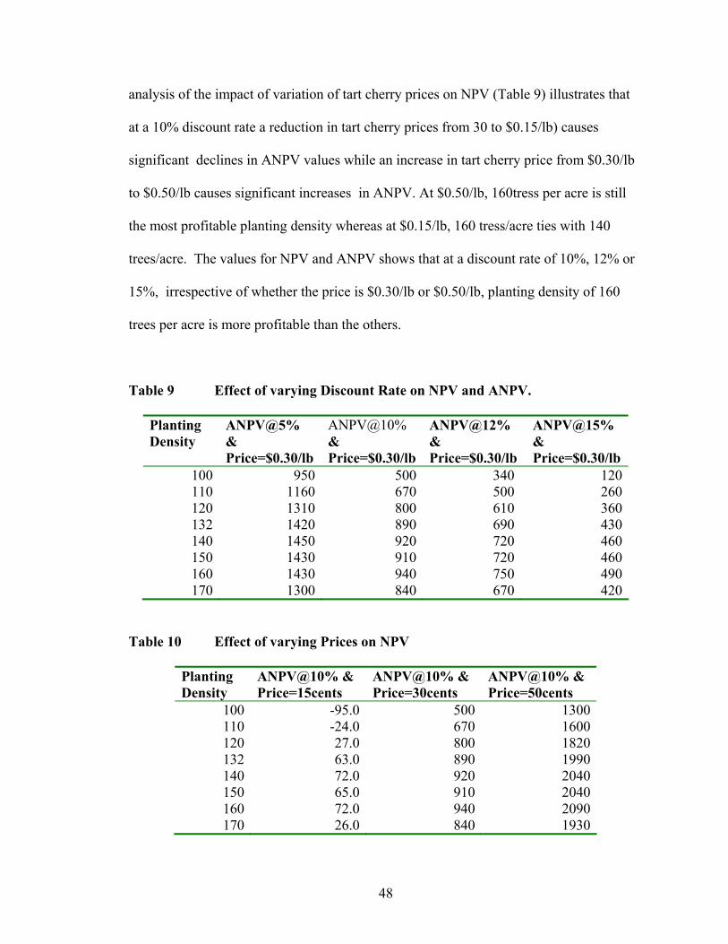
48

analysis of the impact of variation of tart cherry prices on NPV (Table 9) illustrates that

at a 10% discount rate a reduction in tart cherry prices from 30 to $0.15/lb) causes

significant declines in ANPV values while an increase in tart cherry price from $0.30/lb

to $0.50/lb causes significant increases in ANPV. At $0.50/lb, 160tress per acre is still

the most profitable planting density whereas at $0.15/lb, 160 tress/acre ties with 140

trees/acre. The values for NPV and ANPV shows that at a discount rate of 10%, 12% or

15%, irrespective of whether the price is $0.30/lb or $0.50/lb, planting density of 160

trees per acre is more profitable than the others.

Table 9 Effect of varying Discount Rate on NPV and ANPV.

Planting Density

ANPV@5% & Price=$0.30/lb

ANPV@10% & Price=$0.30/lb

ANPV@12% & Price=$0.30/lb

ANPV@15% & Price=$0.30/lb

100 950 500 340 120110 1160 670 500 260120 1310 800 610 360132 1420 890 690 430140 1450 920 720 460150 1430 910 720 460160 1430 940 750 490170 1300 840 670 420

Table 10 Effect of varying Prices on NPV

Planting Density

ANPV@10% & Price=15cents

ANPV@10% & Price=30cents

ANPV@10% & Price=50cents

100 -95.0 500 1300110 -24.0 670 1600120 27.0 800 1820132 63.0 890 1990140 72.0 920 2040150 65.0 910 2040160 72.0 940 2090170 26.0 840 1930

49

SUMMARY OF FINDINGS, CHALLENGES AND RECOMMENDATIONS

This study sought to investigate how variations in planting density influence the

trajectory of yields per acre over the lifetime of a tart cherry block and the corresponding

effects on the profitability of tart cherry production as measured by the ANPV. The study

had four objectives. The first objective was to estimate the joint response of tart cherry

yields to tree age and planting density. A statistical model for the joint response of tart

cherry yield to tree age and planting density was developed and estimated. Results of the

statistical model illustrate variation in the tart cherry yield-age trajectory with planting

densities. It is found that pre-peak, higher planting densities give higher yields (steeper

slope) than lower planting densities. However, post-peak, yields at higher planting

densities decline much faster than those at lower planting densities.

The data used for this study had few observations in stage 4 of the hypothesized tart

cherry yield age trajectory, which illustrates evidence of potential selection bias because

the trees were already pulled out. Consequently it was not possible to capture the shape of

the trajectory in stage 4. Nevertheless, comparing the tart cherry yield age trajectory

estimated by Kessler and Nugent (figure 3) to that estimated here(figure 8) for

consistency, we see that figure 8 reveals a much more linear structure for stage 1 of the

lifecycle than figure 3. Looking at the residuals in figure 7b, there is no compelling

evidence (residuals are randomly distributed around age), that yield response to tree age

is not in fact linear. This means that the shape of the trajectory is more linear than

illustrated by the maintained hypothesis by Kessler and Nugent (figure 3).

50

The second objective of the study was to use information from the estimated tart cherry

yield response model to capture how variations in the trajectory of yield due to

variations in planting density translates into variations in cash flows and profitability of

production as measured by ANPV. Results of this economic analysis reveal that at a

discount rate of 10% and tart cherry priced at 30cents a pound, it is most profitable to

plant 160 trees per acre.

The third objective of this study was to conduct a sensitivity analyses to evaluate the

impact of variations in tart cherry prices and interest rates on the optimal planting density

and orchard economic life. The sensitivity analysis revealed that the optimum planting

density did not change when price per pound was changed to 50cents or when the

discount rate was changed to 12% or 15%. From the preceding analysis, it is seen that

planting density has a potential influence on the trajectory of tart cherry yields over the

life of an orchard. However, prevailing (and even expected) tart cherry prices as well as

the discount factor which reflects the cost of capital are relevant in choosing the most

profitable planting density. The impact of planting density on the economic life of the

block (optimal rotation period) could not be investigated because the data series used in

the analysis was not long enough to verify this effect. This problem was aggravated by

the unbalanced nature of the data which led to the exclusion of blocks that were

incomplete to capture the pattern.

The fourth and final objective of the study was to make recommendations on the

economically profitable planting density. The results reveal that, for large scale farmers

51

in Northwest Michigan, it is most profitable to plant 160 trees per acre when tart cherries

are priced at 30 cents a pound and at a discount factor of 10%. Prevailing (and even

expected) tart cherry prices and/or the discount factor are of course relevant in choosing

the most profitable planting density.

Two challenges were encountered in the course of this study. There is a potential

problem of sample selection bias. Little is known about how the blocks used in the

analysis were selected. Another problem is the lack of data on fruit quality. This made it

difficult to use the effective market prices (prices adjusted for fruit quality) in the

calculation of gross revenue

The unbalanced nature of the data led to dropping of some data which if were complete

would have been very useful in understanding more precisely the effect of planting

density on the trajectory of tart cherry yields. Moreover, few observations, particularly on

the low density end made it difficult to see clearly what happens to the yield-age

trajectory at low planting density. Even more, yields never really turned down. This

made it hard to see the shape of the trajectory in the later stages of the lifecycle as well as

determine the life of the tree. Finally, site quality was identified to be an important factor

that determines what statistical methods to use in the analysis. Variations in site quality

can lead to variation in both the slope and the intercept of the tart cherry yield-age

trajectory. What statistical method to use depends on whether or not we treat site as

random or known. Lack of perfect information on site quality prevented a proper

investigation of the extent to which site quality can influence tart cherry yield-age

52

trajectory. As a result, the study treats site as given, thus allowing for the shape of the

trajectory to be influenced by tree age and planting density. Yields at all planting

densities are constrained to peak at 12 years and only the slope of the trajectory and not

the intercept is allowed to change with planting density.

The preceding statistical analysis allows variation in slopes but constrains the origin of

the tart cherry yield-age trajectory as planting density changes. As such, the method used

in this study could be perceived as a constrained/specialized random coefficient model

which goes beyond the standard random coefficient model (which allows variation in

both the intercept and the slope coefficient), but was still variance components to useful

in achieving part of the reason for the statistical estimation, which was to estimate the

help in the economic model.

53

REFERENCES

Bernarz, C. W. Don Shurley, W., Anthony, W. S. and Nichols, R. L. 2005. Yield, Quality and Profitability of Cotton Produced at Varying Planting Densities. Agronomy Journal Volume 97:235-240.

Black, Roy J. Professor, Agricultural, Food and Resource Economics, Michigan State University. 2009. Personal Communication by author. January 22, East Lansing, MI.

Black J. Roy, James Nugent, Nikki Rothwell, Suzanne Thornsbury, and Nicole Olynk

“Cost of Tart cherry Production in Michigan”. Forth coming Michigan Extension Bulletin. E11/08

Cherry Industry Administrative Board (CIAB). 2009 “Michigan Regional tart cherry

production data”. http://www.cherryboard.org/default.htm. (Accessed on August 10, 2009).

Crawford, E.W. “Agricultural Cost-Benefit Analysis” (Lecture, Michigan State

University, East Lansing, MI, Spring, 2007) French, B.C. and J.L. Matthews. 1971. A Supply Response Model for Perennial Crops. American Journal of Agricultural Economics 53:478-90. French, Ben. C., Gordon A. King, and Dwight D. Minami. 1995. Planting and Removal

Relationships for Perennial Crops: an Application to Cling Peaches. American Journal of Agricultural Economics 67:215-23.

Goedegebure, J. (1991) Business Economic Aspects of High Density Orchards.

Erwerbsobstbau 33, 196-199 Goedegebure, J. (1993) Economic Aspects of Super Intensive Apple Orchards. ISHS

Acta Horticulturae 349:285-293 Greene, H. William. 2007 . Econometric Analysis. 5th Edition. Englewood Cliffs Prentice Hall. Kessler, C. and J. Nugent, unpublished. National Agricultural Statistical Service (NASS), USDA. 2009. “Annual price received

for Tart Cherries”,. http://www.nass.usda.gov/QuickStats/Create_Federal_All.jsp#top (Accessed on August 10, 2009)

54

Ngouanjio, M., Wang, G and Hausbeck, M. K. 2006. Changes in Pickling Cucumber Yield and Economic Value in Response to Planting Densities. Crop Sciences 46: 1570-1575

Pollack, S and Perez, A. 2008 Fruit and Tree Nuts Situation and Outlook Yearbook 2008. U.S. Department of Agriculture, Economic Research Service. FTS-2008. http://www.ers.usda.gov/Publications/FTS/Yearbook08/FTS2008.pdf (Accessed on August 10, 2009).

Pederson, Glenn. 1998. Cost of Capital for Agricultural Cooperatives.

U.S. Department of Agriculture, Rural Business- Cooperative Service. RBS Research Report 163.

Rae, A. N. and Carman, H. F. 1975. A Model of New Zealand Apple Supply Response to

Technological Change. Australian Journal of Agricultural Economics Volume 19:39-51

Robinson, T.L., DeMarree, A.M. and Hoying, S. 2007 An Economic Comparison of Five

High Density Apple Planting Systems. ISHS Acta Horticulturae 732:481-486. Ross, S.A., R.W. Westerfield, and J. Jaffe. 2005 . Corporate Finance . 7th Edition.

Irwin, McGraw-Hill:, Seiter, S., Altemose, C. E. and Davis M. H. 2004. Forage Soybean Yield and Quality

Responses to Plant Density and Row Distance. Agronomy Journal Volume 96:966-970

Springer, T. I. and Gillen, r. L. 2007. How does planting Density Affects the Yield,

quality, and Canopy of native Bluestem ( Andropogon spp.) Forage? Crop Sciences Volume 47:77-82

Wade,L.J and Douglas,A.C.L. 1990. “The Effects of Plant Density on Grain Yield and

Yield Stability of Sorghum Hybrids Differing in Maturity.” Australian Journal of Experimental Agriculture volume 30, 257-64

Wolf, C., S. Hanson, E. Wittenberg and S. Harsh. 2002. Discount Rates for Dairy Farms. Michigan State University, Agricultural Economics Staff Paper 02-08.