AFRL-HE-WP-TR-1999-0214

UNITED STATES AIR FORCE RESEARCH LABORATORY

HSM-PC Users Guide

David J. Pancratz Linda J. Rogers

John B. Bomar, Jr.

BIODYNAMICS RESEARCH CORPORATION 9901IH 10 West, Suite 1000

San Antonio TX 78230

September 1998

wmmm

Interim Report for the Period May 1996 to September 1998

20000215 028

Approved for public release; distribution is unlimited.

oncquM»»'",w<OTBX

Human Effectiveness Directorate Biodynamics and Protection Division Biodynamics and Acceleration Branch 2800 Q Street, Bldg 824 Rm 206 Wright-Patterson AFB OH 45433-7947

NOTICES

When US Government drawings, specifications of other data are used for any purpose other than a definitely related Government procurement operation, the Government thereby incurs no responsibility nor any obligation whatsoever, and the fact that the Government may have formulated, furnished, or in any way supplied the said drawings, specifications or other data, is not to be regarded by implication or otherwise, as in any manner licensing the holder or any other person or corporation, or conveying any rights or permission to manufacture, use, or sell any patented invention that may in any way be related thereto.

Please do not request copies of this report from the Air Force Research Laboratory. Additional copies may be purchased from:

National Technical Information Services 5285 Port Royal Road Springfield, Virginia 22161

Federal Government agencies registered with the Defense Technical Information Center should direct requests for copies of this report to:

Defense Technical Information Center 8725 John J. Kingman Rd STE 0944 Ft. Belvoir, VA 22060-6218

TECHNICAL REVHCW AND APPROVAL

DISCLAIMER

This Technical Report is published as received and has not been edited by the technical editing staff of the Air Force Research Laboratory.

AFRL-HE-WP-TR-1999-0214

This report has been reviewed by the Office of Public Affairs (PA) and is releasable to the National Technical Information Service (NITS). At NTIS, it will be available to the general public, including foreign nations.

This technical report has been reviewed and is approved for publication.

FOR THE DIRECTOR

ROGER L. STORK, Colonel, USAF, BSC Chief Biodynamics and Protection Division Human Effectiveness Directorate Air Force Research Laboratory

REPORT DOCUMENTATION PAGE Form Approved OMB No. 0704-0188

Public reporting burden for this collection of information is estimated to average 1 hour per response, including the time for reviewing instructions, searching existing data sources, gathering and maintaining the data needed and completing and reviewing the collection of information. Send comments regarding this burden estimate or any other aspect of this collection of information, including suggestions for reducing this burden, to Washington Headquarters Services, Directorate for Information Operations and Reports, 1215 Jefferson Davis Highway, Suite 1204, Arlington, VA 22202-4302, and to the Office of Management and Budget, Paperwork Reduction Project (0704-0 188), Washington, DC 20503 1. AGENCY USE ONLY (Leave Blank) 2. REPORT DATE

September 1998 3. REPORT TYPE AND DATES COVERED Interim Report May 1996 to September 1998

4. TITLE AND SUBTITLE HSM-PC Users Guide

6. AUTHOR(S)

David J. Pancratz, Linda J. Rogers, John B. Bomar, Jr.

5. FUNDING NUMBERS C: F41624-96-C-6010 PR: 3005 TA: 300SCB WU: 3005CB62 PE: 6S502F

7. PERFORMING ORGANIZATION NAME(S) AND ADDRESS(ES) Biodynamics Research Corporation 9901IH 10 West Suite 1000 San Antonio TX 78230

8. PERFORMING ORGANIZATION REPORT NUMBER

9. SPONSORING/MONITORING AGENCY NAME(S) AND ADDRESS(ES) Air Force Research Laboratory Human Effectiveness Directorate Biodynamics and Protection Division Air Force Materiel Command Wright-Patterson AFB OH 45433-7901

10. SPONSORING/MONITORING AGENCY REPORT NUMBER

AFRL-HE-WP-TR-1999-0214

11. SUPPLEMENTARY NOTES

12a. DISTRIBUTION/AVAILABILITY STATEMENT

Approved for public release; distribution is unlimited

12b. DISTRIBUTION CODE

13. ABSTRACT (Maximum 200 words) The Head-Spine Model (HSM) originally developed for the Unix environment was recoded for the personal computer. This recode included code improvements and bug fixes, as well as the development of a graphical interface for creating simulations. The HSM can be used to predict the forces and motions of a human spinal column. The vertebrae are modeled with rigid bodies while hydrodynamic elements model the intevertebral discs. A full set of ligamenteous and active muscular models is also incorporated. External accelerations can be applied to the system and the resulting response calculated. A novel method of calculating an initial equilibrium position was incorporated. Several simulations of frontal and vertical accelerations were conducted to demonstrate the utility of the software. Along with the HSM, a database of spinal element properties was created. This database can be separately used from the software to determine mass, material, and geometric properties of the spinal elements as derived from a variety of sources in the literature. This report details the operation of the GUI interface to create, edit, and run simulations.

14. SUBJECT TERMS Spine, Cervical, Simulation, Muscle, Multi-body, Rigid-body

15. NUMBER OF PAGES

3Q- 16. PRICE CODE

17. SECURITY CLASSIFICATION OF REPORT

Unclassified

18. SECURITY CLASSIFICATION OF THIS PAGE

Unclassified

19. SECURITY CLASSIFICATION OF ABSTRACT

Unclassified

10. LIMITATION OF ABSTRACT

UNLIMITED

NSN 7540-01-280-5500 Computer Generated 1996

Standard Form 298 (Rev. 2-89) Prescribed by ANSI Std. 239-18

298-102

This Page Intentionally Left Blank

IX

PREFACE

The investigations described in this report were conducted by the Biodynamics Research Corporation, 9901 I-10 West, Suite 1000, San Antonio TX, 78230. This work was supported with funds from an Air Force SBER Phase II contract number F41624-96-C-6010 from May 1996 to September 1998. The project manager was Dr. Joseph Pellettiere, AFRL/HEPA.

This research builds upon the original HSM code and initial PC porting described in the Phase I report. For additional information please refer to the companion report, A Personal Computer-Based Head-Spine Model, AFRL-HE-WP-TR- 1999-0175

The members of the research team express their deep appreciation to the many individuals and organizations making contributions to this research program. Without the timely assistance given so generously by everyone, the research program and this report could not possibly have been accomplished.

The research team wishes to express their gratitude for the cooperation, support, and guidance of the Air Force Technical Project Manager Dr. Louise Obergefell and Dr. Ints Kaleps of the Human Effectiveness Directorate, USAF Research Laboratory (AFRL).

Finally, the research team gives a very special thank you to the support staff at BRC. Without the effort of Celina Canales in operations support, this research program could not have been reported effectively. Appreciation is also due to Dr. James Raddin and Dr. McConnell for their technical support, Darrin Smith for engineering support, John Martini and Adolph Mena for illustration support, and Patricia Riley for information services support.

in

Contents

Overview ^ History 1

User Guide Organization 2

Installation 3

What You Need 3

Installing HSM 3

Removing HSM 4

User Interface 5

Screen Layout -* Menu Bar 6

Toolbar 6

Tabs 7

Simulation Wizard 8

Creating a New Simulation 8

Editing Parameters 11

Edit Menu U

Editing Model Parameters ^2

Editing Environment Parameters 13 Editing Forcing Function Parameters 16 Editing Simulation Parameters 18

Running a Simulation 20

The Run Option 20

Plotting Output Values 21

Plotting Options 21

Animation 22

Simulation Animation 22

HSM-PC Database 24

Background 24

Interface 24

Index 26

IV

Overview

History The Head Spine Model (HSM) was originally developed by the USAF Aeromedical Research Laboratory during the late seventies. The HSM was created to aid the solution of problems related to spinal loads resulting from ejection seat acceleration.

Biodynamic Research Corporation contracted with the USAF to create a computer model of the dynamic response of the human head and spine that executes on a PC compatible computer under a Windows environment. The HSM-PC is aimed at creating simulations of the biomechanical responses of the head and spine to potentially traumatic impulsive acceleration and impact events (see HSM-PC Final Report).

User Guide Organization

Chapter Description

Overview

Installation

User Interface

The Simulation Wizard

Editing Parameters

Running a Simulation

Plotting Output Values

Animation

HSM-PC Database

The history of the Head-Spine Model and a documentation overview.

A description of HSM-PC system requirements, installation procedures and the uninstall procedure.

A description of the major features of the user interface including the menu bar, toolbars, and tabs.

How to design a simulation by specifying the model elements, the environment, and the simulation parameters.

A description of the mechanism for editing various parameters in a simulation.

How to run a simulation once you have all the specifications assigned.

An overview of the plotting facilities included in HSM-PC.

A description of the animation capabilities of HSM-PC.

A description of the HSM-PC database and its customization options.

Installation

What You Need HSM-PC is a native 32-bit Windows applications designed to install with a 32-bit operating system.

Before you begin installing HSM, make sure you have

• An IBM PC or compatible with a 486 or Pentium-class microprocessor and 8 megabytes of RAM (16 recommended) and a mouse.

• The HSM CD-ROM or floppy disks.

• Windows 95/98 or Windows NT 4.0 (or higher) on your system.

• Approximately 15 megabytes of available hard disk space.

Installing HSM This section describes how to install HSM on a stand-alone system.

To install HSM:

1. Run Windows.

2. Put the HSM CD ROM into your CD ROM drive.

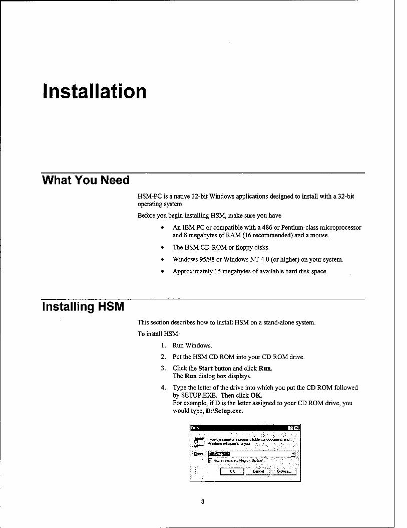
3. Click the Start button and click Run. The Run dialog box displays.

4. Type the letter of the drive into which you put the CD ROM followed bySETUP.EXE. Then click OK. For example, if D is the letter assigned to your CD ROM drive, you would type, D:\Setup.exe.

; J^^ -type *e nameof a program; folded a documentja*Kk. ■..:'.. ^ i Windows wl open it for you

flpert |l>m£UIHiUJ ^jf

F RunmSe~?-ay MerrorvSpace-.

[ OK ] Cancel' *|p frowse.- |

The Setup Information screen displays.

5. Read this screen and click OK. The HSM Directory dialog box displays. In this dialog box you can select the directory in which you want to install HSM. The default is C:\Program Files\HSM.

6. To install:

A) To the default directory, click the large square button on the dialog.

7.

r.s HsmZ Setup

Beshihe retalation byefckino. Ihe button beta*.

Cfc* «s button to raid HOT2 Mlhwre lo It» «peered dettnabon dreday.

Oiectay:

C\PiogrtmFlej\Htm2\ £tange Dfoctoiy

EjotSstw

-OR-

(B) To specify another directory, click the Change Directory button and type the full path in which you want to install HSM.

When you have selected a path, click OK. You will see a status bar indicating the progress of the install. Then you will see a message informing you that the setup is complete.

Click OK.

Removing HSM

This section describes how to remove all HSM program files from your system.

Run Windows as you normally would.

Click the Start button and point to Settings. In the Settings folder,

1.

2.

3.

4.

5.

click Control Panel.

Double-click the Add/Remove Programs icon. The Add/Remove Programs Properties dialog box displays.

Click the Install/Uninstall button.

In the Uninstall list box, click HSM and click the Add/Remove button. The Uninstall HSM dialog box asking if you want to remove the HSM program and all of its files displays.

Click Remove to remove all HSM files from your system.

User Interface

Screen Layout

Tabs

B» eilt tun IT»- loot »t> MdeJttlrtMatrlcUittt •

I s* Bl 6?-l ►! »I Co! If "<" " -'gCC *>*.r-»™-i

Menu Bar

Toolbar

The HSM-PC Menu Bar is always visible within HSM-PC. It contains five drop- down menus:

• The File menu contains New, Open, Close, Save, Save As, and Exit options.

• The Edit menu allows you access to property screens for the simulation parameters.

• The Run menu is used to initiate the computational portion of the simulation.

• The View menu is used to evaluate the results of the simulation. It includes options for Animation or Plotting data.

• The Tools menu allows the user to access either the Calculator or a Text Editor.

• The Help menu gives you quick access to the Help Index and version information.

Status information is displayed on the Menu Bar to the right of the Help option.

Many of the essential HSM-PC tools are included on the toolbar, which is located at the top of the main HSM-PC window. While some of these buttons should be very familiar to you from other Windows applications, others will be new to you.

£ 0 New Open Save Properties Run Animation Editor Help

Name

New

Open

Save

Properties

Run

Animation

Editor

Help

Function

Create a new the simulation.

Open an existing simulation.

Save the current simulation.

Shows a drop-down menu of property dialogs.

Runs the computational portion of the program.

Loads animation data and displays the animation toolbar.

Opens the text editor.

Opens the help file.

Tabs The tabs at the lower left comer of the screen give you access to either viewing the graphical representation of the Head-Spine model or viewing plots of the output data from the simulation.

11. Model | Rotting

Simulation Wizard

Creating a New Simulation Creating a simulation is a 5-step process. The Simulation Wizard walks the user through five screens and indicates the options available. Along with each step in the simulation specification process a separate text file is generated. These files can later be reused in designing future simulations. The initial wizard screen is shown below.

Simulation Parameters In Step 1 the simulation times, units, and print style are specified. The Starting Time and Ending Time are needed to determine the simulation duration. The Print Interval indicates how often data is recorded in the output file. The Units option is used to specify units for the user interface and the output file. Print Style indicates whether all values are recorded at each time step, or the output values are grouped by element. The Step-by-Step mode is an option to facilitate debugging when the computational portion of the program does not run to completion. The Step-by-Step Print Style enables the user to determine at what point the computation failed and what values were recorded just before the failure.

3** Simulation Parameters - Step 1

Speetf the Simulation Tim« and Prä* Interval for Output

Starting Time: | 0.oo (sec)

Ending Time: |

Print Interval: |

025 (sec)

0 01 (sec)

-UMtt- "-

! C Metric (kg-m-sec) !

r English (ib-ftsec)

<*■ Nonrial

C' Step-by-Step

<8«ck ■:|te;Ne*t>-'.l| . uinea ] .

The file containing simulation parameters is referred to as the Input File. As you leave this dialog you will be asked if you wish to use an existing Initialization File or generate a new one. The Initialization File contains data for the model during the initial settling period. When an Initialization File is reused, time is saved on the computations.

Selecting A Model In Step 2 the simulation model is selected. There is a choice of three different models. The first model, Selected Vertebrae, allows the user to select a range of vertebrae to include in the simulation. When this option is selected a list box of all rigid bodies is displayed and the range of vertebrae can be selected. The second model, Head-Cervical Spine, includes the head, cervical spine, Tl, and representations of the viscera. The third model, Head Spine, includes the head, all vertebrae from Cl to L5, the ribs, the pelvis, and representations of the viscera. The file containing the parameters for the elements of the selected model is referred to as the Elements File.

S Simulation Model - Step 2

Spedlythe Biomechanicil Modal you would Oce to u*»for4he Simulation, i

Select Model

<f JHead-Cetvical Spine Model (HCSM)

r Simplified Spine Model with HCSM

C Isolated bgamentous Spine Model with HCSM

r Head-Spine Model (HSM-PC)

MecStv Mcctel Sanenis '

«flack tiext> Cancel!

Specifying the Environment In Step 3 the environment is specified by adding Rigid Bodies, Springs, Planes and Constraints to the simulation. Rigid Bodies, Springs and Planes can be used to represent restraint systems and occupant seating. Planes are required for the application of forcing functions during the simulation. Constraints are used to constrain the motion of a rigid body in any dimension. The file containing the parameters for Rigid Bodies, Springs, Planes and Constraints is referred to as the Environment file.

] External Element Properties - Step 3 Specüy the etcaMot» otthe «ttemal

Bioid Bodies! Spring» T Ptoe» I - 5"?*^

Global ' CooidBate(>: y value. 1 0.000 -met«*

«i.vakje'il 0 000 meter» -Secondary Hodei-

rÄdd3

i . • xvelue [000 met«« -"T\' 'Local . i ___' -1 Coordinate» lvalue 0000 meter«

s value 1 0000 meter*

| Delete | <B»ck 1 ijai> | ■ .Cancd |

Defining Forcing Functions In Step 4 Forcing Functions can be defined. There are two types of Forcing Functions that can be applied to the planes of a simulation. The user can select from a set of Standard Functions (rectangle, triangle, sinusoid, and haversine) or design their own. The functions can be defined as a Position, Velocity or Acceleration. The user must also define a Direction Vector for the plane of the forcing function. User defined functions can be supplied from a text file or by utilizing a Spreadsheet that is provided with the program. The file containing forcing function information is referred to as the Forcing Function file.

Forcing Function Definition

Specify Facing Function* lo bo applied to plane* during the »nutation.

General -

CunentPlane:

Standard Functions Spreadsheet

ill - Style 1

j C Standard Function i

I <* rUset Darned Fincbori

Type

C Posten

r Vetocjy

<• Acceleration

Delete

| X I 000. 'meters

! Y 1 000

2 | 0.00=

meters

mete«

-■'. | Cancel |

Specifying Output In Step 5 the data for the Output file is specified. The elements and appropriate data values that will be recorded in the Output file are selected using the dialog shown below. Use the check boxes to select the parameters to be recorded and the list box to select the elements. The Output file will contain data for each recorded value of each selected element at each time step.

I Output File Format - Step S

Specify Output Parameter! f« this Mutation run.

f Discs ' T Hjrfrooiinww: J External Elements

HioidBodiM T Muscles ] Ligaments

j Posftion hVeloeils. F AcceJefebon r Orientation

r!>nguWVeloc^i P" Angular Acceleration

ALL Head Cervical 1 Cervical 2 Cervical 3 CervicaM Cervica|5

j

<a«ck »? Cancel i'

10

Editing Parameters

Edit Menu To edit the parameters of a simulation, either click the select Edit from the Main Menu.

S* toolbar button or

The pull-down menu on the right will be displayed. This menu gives access to the dialog boxes for editing various parameters of the simulation run. It also displays the names of the text files used to store the parameter values. If the file name is selected, a Save As dialog will be displayed and the name of the text file can be changed.

0 Model 9ELEM.TXT

;p £nvtonment

ENVIR0N8TXT

}p Forcing Function

3N0DE.SIM

f£j Timing Parameters

p Qutput Parameters

0 0UT88.TXT

11

Editing Model Parameters When Model is selected from the Edit pull-down menu the Model Properties dialog is displayed. The Model Properties dialog has a tab for each type of element in the model. The specific element for that type can be selected from a combo box at the top of the tab and then the properties for that element will be displayed below. These properties are read from the HSM-PC database. The properties are displayed in the units which were selected for that simulation.

RvcBain | Mjun- «M Dacs | fxth | Vn»<i| ~J\

BlotuiCoonfcnal« Mo««* of Imrtu

>vak» j o:M man 1 00333 kBAiT2

»vdue | ao rutaj >«s| 0(0S4 kjM-2

last a^/_ ksfcft Socond«j Nodet

*' |RisHocopiUlcmtte(i!a<taiKP«t)

Cooidmxet »"*"

ivafc»

| -0018 »K

| 002 „am

| a«2 rom

12

Editing Environment Parameters When Environment is selected from the Edit pull-down menu, the External Element Properties dialog is displayed. This dialog has a tab for each type of element in the environment (Rigid Bodies, Springs, and Planes) and a tab for specifying Constraints on Rigid Bodies in the model. To add new elements to the environment, use the Add button at the bottom of the dialog. To remove an element, first select it in the list box above and then use the Delete button at the bottom of the dialog. To save the changes, select the OK button. To exit without saving, use the Cancel button.

r\ External Element Properties Spcrity the el«»«*» of the mdeinal onvkonteent

ff RUdBodat T Springs f Planes ] Constraint!

6lobal "*"° Coordmate* value

* '• lvalue

1 0000 „stew

| 0 000 mete»

| 0000 meters _ ■ ■■ • > i *'

\ -I . . xvakitf'H...

>■■" | Local r- 0000 ma«,

0000 raters

0000 meters Lootdnata* yy«*je |

"" " 'rvalue |

|! Add l| Delete | UK. | Cancel |

Rigid Bodies

To define a Rigid Body, select the Rigid Bodies tab and press the Add button at the bottom of the dialog. You will be prompted for a name for the rigid body. Next, enter the x, y, and z coordinate values of the primary node for that rigid body using global coordinates. Once a primary node has been defined, secondary nodes for that rigid body can be added using the Add button under the Secondary Nodes list box. Again you will be prompted for a name for each secondary node. After the node has been named, enter the x, y, and z coordinate values (in local coordinates) in the fields provided on the right.

External Element Properties Specifj( «he Bleuem» of the

Rigid Bodies T Springs 1 Planes T CondtaWt

Vehicle Flora

^Secondary Nodes-

^filooal s*vakies

Coordinates yvake 1 000 jmetetsi;

lvalue I 1.000 jmetere

>Vakjevi

Coordinates »value 4.000 meters

rvalue | 4.000 meters

/Add Dotete m& iCanceta

13

Springs

To define a Spring in the environment, select the Springs tab and press the Add , button at the bottom of the dialog. You will be prompted for a name for the Spring and the name will be added to the list box. Now the type of Spring can be selected along with its Kl and K2 values. The end points are selected from a list of primary and secondary nodes.

External Element Properties Specify the eteownU of the «denial envireraeenL

Rigid Bod« f Spring. T Plane» ] Constrarts

Type

r r tension r both

Kl

K2

Ufa -EndPdnts "3: -3

Add Delete SK |Emoä:ii

Planes To define a Plane in the environment, select the Planes tab and press the Add button at the bottom of the dialog. You will be prompted for Plane number and the number will be added to the list box. Now the coordinates for the three points defining the plane can be entered. The Tab key will position the cursor for entering x, y, and z for point 1 and similarly for point 2 and point 3. Then stiffness to deflection and stiffness to deflection rate can be entered. If any of the values need to be adjusted, simply position the cursor on the appropriate field and enter the new value. Any Planes that are defined for the environment can later be used in defining forcing functions.

■-.— ~~ - - ~ " " ■■■■■:■■■

r7; External Element Properties «Ul Specif» the element* of the external environment

fiioidBodes T Spnngs T Plant T Constraints

Stiffness to Deflection 1 OKI NAn

Sfifness to Deflection Rate | Ö.Ö0 N/iti

Pointl PoW2 Pomf3

»value 1 OP00 meters 1 .9-°9° meters 1 °°°° meters

yvata I 0.000 itneter« | 0.000 meters | 0.000 meters

zvabe | 6.000 -meters | 0.000 mete« | 0.000 meters

Add j' Delete | ' flK | "Cancel |

14

Constraints

To define a Constraint for a rigid body, select the Constraints tab and press the Add button at the bottom of the dialog. You will be prompted for Constraint number and the number will be added to the list box. Next select the Rigid Body that you wish to constrain. Use the check boxes at the lower part of the dialog to indicate the motion requiring Constraint.

External Element Properties Spwafjf theelatenttottha external envirotwünt.

ifiigidBoaw.lf SpcSngt "If ""«~"l CoWrainht

W VotebieAopiedto

II

Constrained Motion:

TX rAngutorX

TY TAnoviBY.

T2 rAnautaZ

'■mi Delete txmM

15

Editing Forcing Function Parameters

When Forcing Function is selected from the Edit pull-down menu, the Forcing Function Definition dialog is displayed. To add a new Forcing Function, select a Plane using the arrows at the upper left of the dialog. Once you have selected a Plane you can specify the style, type and direction vector for the function.

Specify Forcing Function lo bo appM to plan» during Ins iswdaaon.

6anaul f SlandaidFunctioro | Spraataoat

Cunant Planet

■Sl* ,

.ff Srend»d Function I

r User Oefred Function :

r-Typ«. ------ C Poation

C Accetobon

DseaionVeclor

met are

tnetsts

roetas

Y

ago,, aoo

2 . w

App» I ■.

Standard Functions

If you select a Standard Function as the style, use the second tab to specify the type of function and the function parameters. For Standard Functions you can select from rectagular, triangular, haversine and sinusoidal. Further you need to specify the begin time, end time, peak time (for triangular functions only), offset, and amplitude.

Specify Forcing Function« lo be applied lo pianos d

J Stared F*»waion*T! Spreadsheet

Siandetd Functions-

(? Rectanoutat

r ToanoJs

C Haversine

r shusodd

Deet» I Apply |

-FureWiPawnetenv-

beontkne | 0.00

endbm» | 0 75

i' '■" * I i

offset | Öröl

emfbujt 1.00..

J Cancel |

16

User Defined Functions

When a User Defined Function is selected, the options are to use a file to define the function or use the Spreadsheet provided by the program. If you opt to use a file you will be prompted for the file name. The file should be a text file with two columns of values. The first column specifies the time and the second column specifies the function value for each time.

Foicmg Function Definition

Specify Forcing Function to bewpiud lopiann during Un

] Spraodtheel 1

Curort Flare.

Ti»! ' $&r±-

C StarrfaidFuWion

<? UtaDefradFuKboT

rT>pe ■

C Paation

' C Accotaetion

Ihot Denied FireSom-

C UseFfe *

ipnadtoet

OrecnonVecax

mete»

x | aoo Y 1 ax

, 2 1 1.00

"DB 1."-ÄH» I -\: IBCencelS

When the Spreadsheet option is selected, select the Spreadsheet tab and enter the data describing the function in the value column of the Spreadsheet. The Spreadsheet includes graphing capability so that you view the function as you enter values into the Spreadsheet. When the Forcing Function Definition is complete the Forcing Function file will be saved for later use.

: Spoof?Fonang Function» to be appSod to plan« during tho sMabon.

««General; ~Y Spräö*hoötj_

Voluo ;;/Vrj:?:i:r^-CllOrt'-"B'.:..N5':-*St <;»± A ■:<■ "" ,

' 2 1

1 ■

,.l» T " " 1 xs

15 15

•r» -

«i- a»,-. ■»»■i 2 2 1.3

* t

•**■■■■ 13

13 13 '1

o- « Ai 1*S 1

Ooloto A(rt> ,Care»f:

17

Editing Simulation Parameters When Simulation is selected from the Edit pull-down menu, a submenu is displayed. The submenu contains options for Timing Parameters and Output Parameters.

[|j?J liming Parameters

[|p Output Parameters

Editing Timing Parameters The dialog for editing the simulation Timing Parameters is the same as the dialog described in the Simulation Wizard for setting up Simulation Parameters. Change any of the values that require updating and then press OK.

^! Simulation Paiaraeteis

Specify tha Smaation Ti

Stating Time |3£3

Ending Time:

Print InteivaJ:

and Print Interval for Output.

(sac)

CL25 (sec)

(sec) am

-Un*»

ff Metric (kg-m-sec)

ri

— Print Style —

C Normal r

■W&eSB

18

Editing Output Parameters The dialog for editing the Output Parameters is shown below. Different element types are displayed on different tabs. Elements from the environment are grouped on the External Elements tab. Use the check boxes to select the parameters to be recorded and the list box to select the elements of interest. Change any of the values that require updating and then press OK.

! Output File Formöt

Specgy Output Patirtara h» thus mutation ran.

f Discs f HjdroajBa ] External Element«

Rigid Bodlas I Mmdet [ Ligaments

1^ .PuuUui

n VeloeJty

I-* Acceleration

[?. Orientation

r Angiiat Acceleiabx :!Ü£^

Head ij CervfcaM f; Cervical 2 fe Cervical3 f: Cervical4 |i CeryicalS...^ _.£

Cancel l|

19

Running a Simulation

The Run Option To initiate the computational portion of HSM-PC, either click the | > toolbar button or select Run Simulation from the Run menu.

During the execution of the simulation the screen will display the time steps as the simulation progresses.

gto £* Sw» SWR Irfhdort &*>' - _

HiH

II äHB^^^^^^^^^^^^H ^l^^l

ifcunoliillH

When the simulation computations are complete a dialog will indicate that the program has terminated and will ask "Exit Window?" Select Yes.

After the simulation has been run the Text Editor will display the Error File to display any messages from the computational run. If the simulation is successful, the user will now be able to review the results. Plotting and animation capabilities are provided, or the output file can be viewed with the Text Editor to observe the raw data values. Although the HSM-PC program does not include features for exporting data, result data can be imported using Microsoft Excel.

20

Plotting Output Values

Plotting Options When the Plotting tab is selected the screen will display the Plotting Screen. On the right-hand portion of the screen are two panels for specifying the Plotting Options. The upper panel has a list of any model elements which have plot values available in the output file. The lower panel has the element values to plot.

iUoMkMHeW*'

D tfBig-: ►!»■!) T!

0.7

0.S

OS

S 04 e a 4 03

02

0.1

■OH

R]g]d Body Oritntstion - Ctrvkal 6

H J

I 1 I

0.1 0.1S

seconds

iMttM m*ai'i\:

Plot Items

Plot Values

The Plot Items Panel displays a hierarchical list of all the model elements which were selected for the output file. A heading will appear for each group of an element type such as Rigid Bodies or Muscles. When the "plus" sign to the left of the heading is clicked, the hierarchy is expanded to show all the specific elements ofthat type. After expansion, the "plus" sign becomes a "minus" sign. To collapse an expanded portion of the hierarchy, click the "minus" sign and the specific elements will no longer be listed. To select model element for plotting, click on the specific element in the expanded hierarchical list.

Once a model element is selected from the Plot Items list, the lower panel will display the values which are available for that model element. Select the value you wish to plot from the Plot Values and the plot ofthat value will be displayed.

21

Animation

Simulation Animation

After the computational portion of the HSM program has been run, the output data can be viewed as an animation. To initiate an Animation either select the Animation option on the View menu or click the Animation button on the toolbar.

The screen will display the animation toolbar on the right-hand side. The model will only display rigid bodies and planes during the Animation sequence. The HSM program uses the SAE coordinate system (Z-axis pointing down and the X-axis pointing forward) when displaying the model.

Animation Toolbar

Animation

Animation

► m « play stop rewind

•Ji Loop Mode

Step Mode

4 ► Step Frames

Speed

Animation The Animation portion of the toolbar allows you to play, stop, and rewind the animation sequence. The Loop Mode button will play the animation sequence continuously until the stop option is selected.

Step Mode The Step Mode portion of the toolbar has tools for stepping through the animation sequence in a forward or backward direction. The Step Frames options allows you to set the number of frames to be advanced with each step.

Speed The Speed portion of the toolbar allows the user to set the rate of the animation sequence. The Time Step of the current frame is also displayed here.

Print Image The Print Image option brings up a dialog which allows the user to select a page layout for printing snap shots from the Animation sequence. The dialog has options for a single image page and two sizes of images on a four image per page layout.

< II.

Time Step: 0.010 sec.

Print Image

Save Image

Camera Mode

22

The dialog will also prompt the user for the bitmap images to use for the page layouts.

Save Image The Save Image option enables the user to download the current screen image to a bitmap file. The user can use the step mode controls to select the desired image and then capture that image using the Save Image option. A Save File dialog will prompt the user for a file name to assign to the bitmap. These saved images are used with the Print Image option described above.

23

HSM-PC Database

Background

The best available anatomic, geometric, and materials data that was available to the development team is included in the database. The data can be altered or added to using Microsoft Access. The HSM-PC Database can be accessed by the HSM-PC program on-line or employed as a stand-alone database on the structure and materials properties of the spine.

The HSM-PC Database was developed using Microsoft Access 97. The data in the database include the coordinates and parameter values used in HSM as well as additional data from the more current literature.

Interface MSB

HüJL'J-Ssinü LXitabase

Cervical Vertebrae,

Thoracic Vertebrae

Lumbar Vertebrae

Exit

24

The database application has a main menu that allows access to data from different areas of the spine. Once a selection has been made from the main menu, individual records from the database can be viewed.

j fS Cervical HBB Vertebra. ßQBRDe'

üÄ^BiPiiiiii

Reference IDoherty and Heggeness (1995)

Numbec of Sample* | 51 Spiral CanalOepth j IE 5

Lower EnrJPIate Depth | 162 Spinal Canal Depth SD | 17

Lower ErxtPlate Depth SD | 1.6 Spinel Canal Area ' |

Lower EndflalevÄtti • | . Spiral Canal Area SD |

Lower EndPlateVfidrhSD | Spncus Process Length ,.j

VertebtatBooVHeight | 23.3 Spirous Piece» Length SO j

Vertebral Body HerghtSD. J 1.9 Trarttver»ft«»»Wiclh | ig

Spnal Canal Width | 23 6 Transverse Process W«*h SD |

SpnalCanalWidthSD | 16

Mutete Record View 1 VBW Only Records for | J

Mi*. K|«1l 2 jjiiJ»» 1 •» 29

The buttons at the lower left corner on the screen allow navigation through the database. From this screen a multiple record view can be selected by pressing the button labeled Multiple Record View.

Vertebra ^flfSIBOCt) Number of , LowerEndflat» Lower Endflate •. «Sample» -Deptti IMiSO •

Lower EnoTtote W«th

MietiEnd^j WidthsJ

► *™ _ Doherty and Happen« (1894) »1 1 1 1 |CHviMl2 Doherty and Heppeness 11335) 51 ( 16.2J 1.S| ,...=1 |Cetvical2 Punjabi. Duanceeu. Goal Oidand.

and lakata [1390] 12j 15B!| 158:) 17.5 |

|CavicBl2 Lanier (1333) 36) 12*J a\ 19 |

|tavical2 ÜU11378] '1 Kl C' "| |Cervical2 Francis |1355) 100] lG.li| ttj 19.5;|

|Cervical 3 Panrabi.Duanceau.Goet Oidand. andTakata(1990)

12( 15.6) Mif 17.2J •- - |CetvicaI3 Lanier (1933) ?.l l"l- -. . -°J 20.31

|Cetvcal3 Liu (1378) 1| 13| 0| "1 , A B m»rt: ;«1 «H i >im»li>r!» «1

25

Index

B

Background 24

H

History 1-2,1-2

I

Interface 2, 6, 9,24

Tabs 2, 8,19 Toolbar 7, 12,20,22

26