
Talisman Energy, capillary pressure, saturation, permeability and NMR Malay Basin Example.pdf
60
Capillary Pressure, Saturation, Permeability and NMR: Malay Basin Example Andrew Logan – Talisman Malaysia Limited FESM November 2008
description
capillary pressure
Transcript of Talisman Energy, capillary pressure, saturation, permeability and NMR Malay Basin Example.pdf
Capillary Pressure, Saturation,
Permeability and NMR: Malay
Basin Example
Andrew Logan – Talisman Malaysia Limited
FESM November 2008

Summary
• Compare methods of modeling capillary pressure (Saturation Height Functions) and demonstrate similarity of Sw results in generic models for the Malay Basin.– Parameters for J-Function, Power Function, Lambda Functions
and Thomeer Method are derived and results compared.
• Use Capillary Pressure data to derive a generic permeability equation based on porosity and irreducible water saturation– Coates Parameters are derived from capillary pressure data.
• Application of NMR in the above models– Some preliminary results
• These three closely related topics gain from being discussed together rather than individually.

• Wetting fluid (usually water) is held in the pore space by capillary forces.
• The wetting fluid is displaced only when the capillary forces are exceeded. Pc arises from density difference between water and hydrocarbon.
• Sw may be estimated by computing the pressure difference due to the “height-above-free water”combined with knowledge of the capillary pressure curve.
– Suitable conversions for fluid types must be applied.
• Fluid contact (i.e. the height above free water) is a key parameter since it impacts Pc.
0
1
2
3
4
5
6
7
8
0 10 20 30 40 50 60 70 80 90 100
Water Saturation, % pore volume
Pre
ss
ure
, b
ar
Review of Capillary Pressure
Well XXXXXX
Fluids Air-Water
Method HS Centrifuge
NOB 800 psi
Klinkenberg Capillary End face
Sample Depth Permeability Porosity Pressure Sw
No. (m) (mD) (frac) (psi) (frac)
XXXX XXXX.XX 1050.00 0.2550 0.00 1.00
1.00 0.57
2.00 0.44
5.00 0.33
10.00 0.26
25.00 0.23
50.00 0.20
100.00 0.20
200.00 0.18
500.00 0.16
750.00 0.16

• It is necessary to make a conversion between Laboratory Conditions,
(fluids used for Pc measurement) and Reservoir conditions with
different fluids. Different fluids have different wettability (surface
tension) properties.
• Typical values for usual reservoir fluids are shown in the table below.
)cos(
)cos(
RESRES
LABLABcREScLAB PP
θσθσ
=
260.86630º30Oil/Water/Solid
-370-0.755140º480Air/Mercury/Solid
7210º72Air/Water/Solid
σσσσcos(θθθθ)cos(θθθθ)θθθθσσσσSystem
Fluid System Conversion

hP oilbrinec )( ρρ −=
• In the reservoir, the
capillary pressure may
be estimated by
computing the pressure
difference due to
different fluid densities
and the “height-above-
free-water”, h.
0
10
20
30
40
50
60
70
80
90
100
0.0 10.0 20.0 30.0 40.0 50.0 60.0 70.0 80.0 90.0 100.0
Water Saturation ( % PV)
He
igh
t A
bo
ve
Fre
e W
ate
r (m
)
Capillary Pressure and Saturation Height Functions

Capillary Pressure Modeling
λc
wirrwP
CSS =−
φθσkP
JJSIS cw
cos
2166.0:)log(* =+=
b
c
wP
aS =
−=
−
dP
cP
G
eSwlog
1
Lambda
Function
J-Function
Power
Function
Thomeer
Parameters

• Capillary pressure curves usually have differing relationships
between Pc and Sw.
– Usually one Cap-pressure curve does not adequately describe a
reservoir.
• Several methods are available to describe Capillary Pressure
Measurements
– J-Function
– Lambda Function
– Thomeer Parameters
– Power Function
• All methods are based on curve fitting with little or no physical
modeling behind them.
– Relationships hint at some underlying physical principles.
• Each may be used to describe capillary pressure, but differ in
implementation.
Modeling Capillary Pressure Data
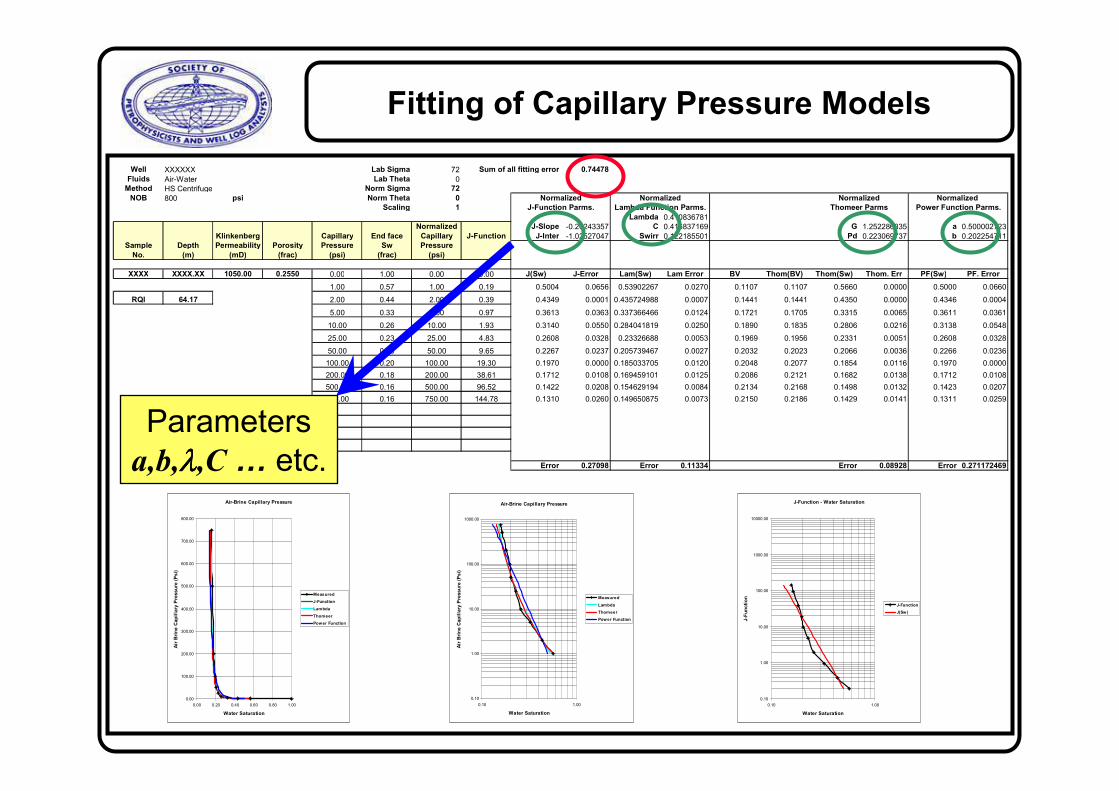
Fitting of Capillary Pressure Models
Well XXXXXX Lab Sigma 72 Sum of all fitting error 0.74478
Fluids Air-Water Lab Theta 0
Method HS Centrifuge Norm Sigma 72
NOB 800 psi Norm Theta 0
Scaling 1
Lambda 0.410836781
Normalized J-Slope -0.20243357 C 0.416837169 G 1.252286835 a 0.500002723
Klinkenberg Capillary End face Capillary J-Function J-Inter -1.02527047 Swirr 0.122185501 Pd 0.223069737 b 0.202254711
Sample Depth Permeability Porosity Pressure Sw Pressure
No. (m) (mD) (frac) (psi) (frac) (psi)
XXXX XXXX.XX 1050.00 0.2550 0.00 1.00 0.00 0.00 J(Sw) J-Error Lam(Sw) Lam Error BV Thom(BV) Thom(Sw) Thom. Err PF(Sw) PF. Error
1.00 0.57 1.00 0.19 0.5004 0.0656 0.53902267 0.0270 0.1107 0.1107 0.5660 0.0000 0.5000 0.0660
RQI 64.17 2.00 0.44 2.00 0.39 0.4349 0.0001 0.435724988 0.0007 0.1441 0.1441 0.4350 0.0000 0.4346 0.0004
5.00 0.33 5.00 0.97 0.3613 0.0363 0.337366466 0.0124 0.1721 0.1705 0.3315 0.0065 0.3611 0.0361
10.00 0.26 10.00 1.93 0.3140 0.0550 0.284041819 0.0250 0.1890 0.1835 0.2806 0.0216 0.3138 0.0548
25.00 0.23 25.00 4.83 0.2608 0.0328 0.23326688 0.0053 0.1969 0.1956 0.2331 0.0051 0.2608 0.0328
50.00 0.20 50.00 9.65 0.2267 0.0237 0.205739467 0.0027 0.2032 0.2023 0.2066 0.0036 0.2266 0.0236
100.00 0.20 100.00 19.30 0.1970 0.0000 0.185033705 0.0120 0.2048 0.2077 0.1854 0.0116 0.1970 0.0000
200.00 0.18 200.00 38.61 0.1712 0.0108 0.169459101 0.0125 0.2086 0.2121 0.1682 0.0138 0.1712 0.0108
500.00 0.16 500.00 96.52 0.1422 0.0208 0.154629194 0.0084 0.2134 0.2168 0.1498 0.0132 0.1423 0.0207
750.00 0.16 750.00 144.78 0.1310 0.0260 0.149650875 0.0073 0.2150 0.2186 0.1429 0.0141 0.1311 0.0259
Error 0.27098 Error 0.11334 Error 0.08928 Error 0.271172469
Normalized
Power Function Parms.
Normalized
Lambda Function Parms.
Normalized
J-Function Parms.
Normalized
Thomeer Parms
Air-Brine Capillary Pressure
0.00
100.00
200.00
300.00
400.00
500.00
600.00
700.00
800.00
0.00 0.20 0.40 0.60 0.80 1.00
Water Saturation
Air
Bri
ne C
apilla
ry P
ressure
(P
si)
Measured
J-Function
Lambda
Thomeer
Power Function
Air-Brine Capillary Pressure
0.10
1.00
10.00
100.00
1000.00
0.10 1.00
Water Saturation
Air
Bri
ne C
apilla
ry P
ressure
(P
si)
Measured
Lambda
Thomeer
Power Function
J-Function - Water Saturation
0.10
1.00
10.00
100.00
1000.00
10000.00
0.10 1.00
Water Saturation
J-F
unction
J-Function
J(Sw)
Parameters
a,b,λλλλ,C� etc.

Table of Fitting Results
Well Sample Depth Lab Sigma Lab Theta Porosity Permeability Swirr C Lamda At 50 psi BVI Error
XXXXXX XXXX XXXX.XX 72 0 0.2160 46.00 0.21 0.78557 0.410837 0.371895 0.080329 0.2029
XXXXXX XXXX XXXX.XX 72 0 0.2180 136.00 0.46 0.525545 0.410837 0.560649 0.122222 0.2148
XXXXXX XXXX XXXX.XX 72 0 0.2030 86.00 0.13 0.75511 0.410837 0.278251 0.056485 0.2531
XXXXXX XXXX XXXX.XX 72 0 0.1800 14.40 0.17 0.830021 0.410837 0.336351 0.060543 0.3642
XXXXXX XXXX XXXX.XX 72 0 0.1090 3.26 0.40 0.798618 0.410837 0.556894 0.060701 0.3021
XXXXXX XXXX XXXX.XX 72 0 0.2390 238.00 0.18 0.378283 0.410837 0.253572 0.060604 0.1402
XXXXXX XXXX XXXX.XX 72 0 0.1840 13.20 0.20 0.81342 0.410837 0.364368 0.067044 0.3513
XXXXXX XXXX XXXX.XX 72 0 0.1850 20.30 0.15 0.850617 0.410837 0.319883 0.059178 0.2827
XXXXXX XXXX XXXX.XX 72 0 0.2290 249.00 0.22 0.388202 0.410837 0.299571 0.068602 0.1019
XXXXXX XXXX XXXX.XX 72 0 0.2150 111.00 0.18 0.562924 0.410837 0.287967 0.061913 0.1281
XXXXXX XXXX XXXX.XX 72 0 0.1900 35.70 0.17 0.788231 0.410837 0.332142 0.063107 0.3604
XXXXXX XXXX XXXX.XX 72 0 0.2560 439.00 0.16 0.341096 0.410837 0.224061 0.05736 0.1056
XXXXXX XXXX XXXX.XX 72 0 0.2550 1050.00 0.12 0.416837 0.410837 0.205739 0.052464 0.1133
XXXXXX XXXX XXXX.XX 72 0 0.2140 51.00 0.15 0.834018 0.410837 0.313839 0.067162 0.1713
XXXXXX XXXX XXXX.XX 72 0 0.2380 236.00 0.18 0.498915 0.410837 0.281581 0.067016 0.1592
XXXXXX XXXX XXXX.XX 72 0 0.2520 417.00 0.03 0.510268 0.410837 0.13486 0.033985 0.4942
XXXXXX XXXX XXXX.XX 72 0 0.2640 479.00 0.12 0.502782 0.410837 0.221984 0.058604 0.3755
XXXXXX XXXX XXXX.XX 72 0 0.1660 19.10 0.19 0.893739 0.410837 0.373563 0.062012 0.5065
XXXXXX XXXX XXXX.XX 72 0 0.2950 1360.00 0.11 0.298678 0.410837 0.16928 0.049937 0.1207
XXXXXX XXXX XXXX.XX 72 0 0.2810 2060.00 0.09 0.184025 0.410837 0.13183 0.037044 0.3138
XXXXXX XXXX XXXX.XX 72 0 0.1240 3.19 0.28 0.882574 0.410837 0.456714 0.056633 0.6406
XXXXXX XXXX XXXX.XX 72 0 0.1530 17.00 0.24 0.64846 0.410837 0.370708 0.056718 0.0850
XXXXXX XXXX XXXX.XX 72 0 0.1910 65.10 0.11 0.853812 0.410837 0.283332 0.054116 0.4561
XXXXXX XXXX XXXX.XX 72 0 0.1600 4.99 0.27 0.967255 0.410837 0.46705 0.074728 0.3846
XXXXXX XXXX XXXX.XX 72 0 0.2750 2740.00 0.05 0.403253 0.410837 0.134785 0.037066 0.1135
XXXXXX XXXX XXXX.XX 72 0 0.2170 493.00 0.20 0.301966 0.410837 0.261622 0.056772 0.2789
XXXXXX XXXX XXXX.XX 72 0 0.1430 65.90 0.31 0.576496 0.410837 0.422643 0.060438 0.5471
XXXXXX XXXX XXXX.XX 72 0 0.2560 1212.00 0.07 0.504979 0.410837 0.169278 0.043335 0.0618
XXXXXX XXXX XXXX.XX 72 0 0.2210 390.00 0.13 0.348139 0.410837 0.202318 0.044712 0.2650
XXXXXX XXXX XXXX.XX 72 0 0.2400 757.00 0.08 0.581892 0.410837 0.193623 0.046469 0.0493
XXXXXX XXXX XXXX.XX 72 0 0.2070 112.00 0.11 0.818213 0.410837 0.273856 0.056688 0.3220
XXXXXX XXXX XXXX.XX 72 0 0.2900 4213.00 0.08 0.446953 0.410837 0.170928 0.049569 0.1138
XXXXXX XXXX XXXX.XX 72 0 0.3090 2143.00 0.14 0.470232 0.410837 0.238535 0.073707 0.1351
XXXXXX XXXX XXXX.XX 72 0 0.2310 240.00 0.18 0.68961 0.410837 0.321134 0.074182 0.2138
Lambda Function Parameters
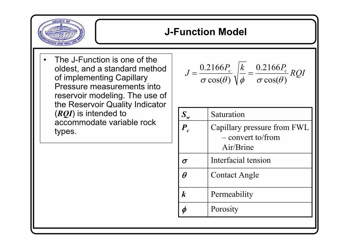
J-Function Model
RQIPkP
J cc
)cos(
2166.0
)cos(
2166.0
θσφθσ==
Porosityφφφφ
Permeabilityk
Contact Angleθθθθ
Interfacial tensionσσσσ
Capillary pressure from FWL
– convert to/from
Air/Brine
Pc
SaturationSw
• The J-Function is one of the oldest, and a standard method of implementing Capillary Pressure measurements into reservoir modeling. The use of the Reservoir Quality Indicator (RQI) is intended to accommodate variable rock types.

J-Function
)log(* JSlopeInterceptSw +=
• For each J-Function, a fit may be computed between the J-Function and Sw. Where the slope and intercept can be used to describe Sw as a function of J.
J-Function - Water Saturation
0.10
1.00
10.00
100.00
1000.00
10000.00
0.10 1.00
Water Saturation
J-F
unction
J-Function
J(Sw)
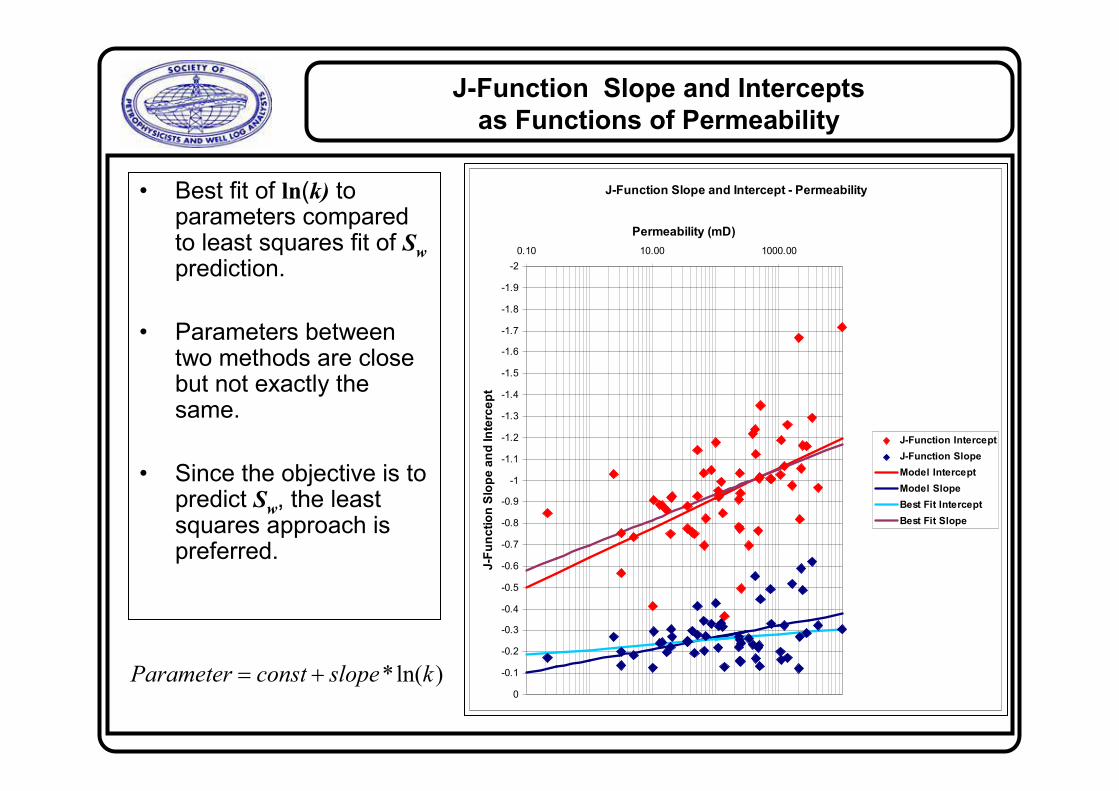
J-Function Slope and Intercepts
as Functions of Permeability
J-Function Slope and Intercept - Permeability
-2
-1.9
-1.8
-1.7
-1.6
-1.5
-1.4
-1.3
-1.2
-1.1
-1
-0.9
-0.8
-0.7
-0.6
-0.5
-0.4
-0.3
-0.2
-0.1
0
0.10 10.00 1000.00
Permeability (mD)
J-F
unction S
lope a
nd Inte
rcept
J-Function Intercept
J-Function Slope
Model Intercept
Model Slope
Best Fit Intercept
Best Fit Slope
• Best fit of ln(k) to parameters compared to least squares fit of Sw
prediction.
• Parameters between two methods are close but not exactly the same.
• Since the objective is to predict Sw, the least squares approach is preferred.
)ln(* kslopeconstParameter +=

Least Squares Fit on all Capillary Pressure Data
to Optimize Model fit – J-Function
Measured Sw vs. Modeled Sw
0.00
0.10
0.20
0.30
0.40
0.50
0.60
0.70
0.80
0.90
1.00
0.0000 0.1000 0.2000 0.3000 0.4000 0.5000 0.6000 0.7000 0.8000 0.9000 1.0000
Permeability Predicted Sw
Capilla
ry P
ressure
Sw
J-Function
• Optimize 4 J-Function Parameters over the entire Capillary Pressure data set.
• Average Error = 0.069
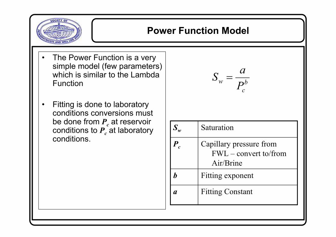
Power Function Model
• The Power Function is a very simple model (few parameters) which is similar to the Lambda Function
• Fitting is done to laboratory conditions conversions must be done from Pc at reservoir conditions to Pc at laboratory conditions.
b
c
wP
aS =
Fitting Constanta
Fitting exponentb
Capillary pressure from
FWL – convert to/from
Air/Brine
Pc
SaturationSw
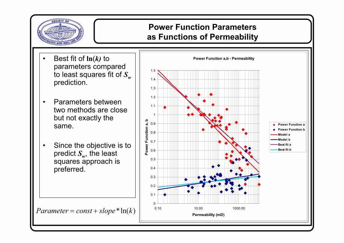
Power Function Parameters
as Functions of Permeability
Power Function a,b - Permeability
0
0.1
0.2
0.3
0.4
0.5
0.6
0.7
0.8
0.9
1
1.1
1.2
1.3
1.4
1.5
0.10 10.00 1000.00
Permeability (mD)
Pow
er Function a
, b
Power Function a
Power Function b
Model a
Model b
Best fit a
Best fit b
)ln(* kslopeconstParameter +=
• Best fit of ln(k) to parameters compared to least squares fit of Sw
prediction.
• Parameters between two methods are close but not exactly the same.
• Since the objective is to predict Sw, the least squares approach is preferred.
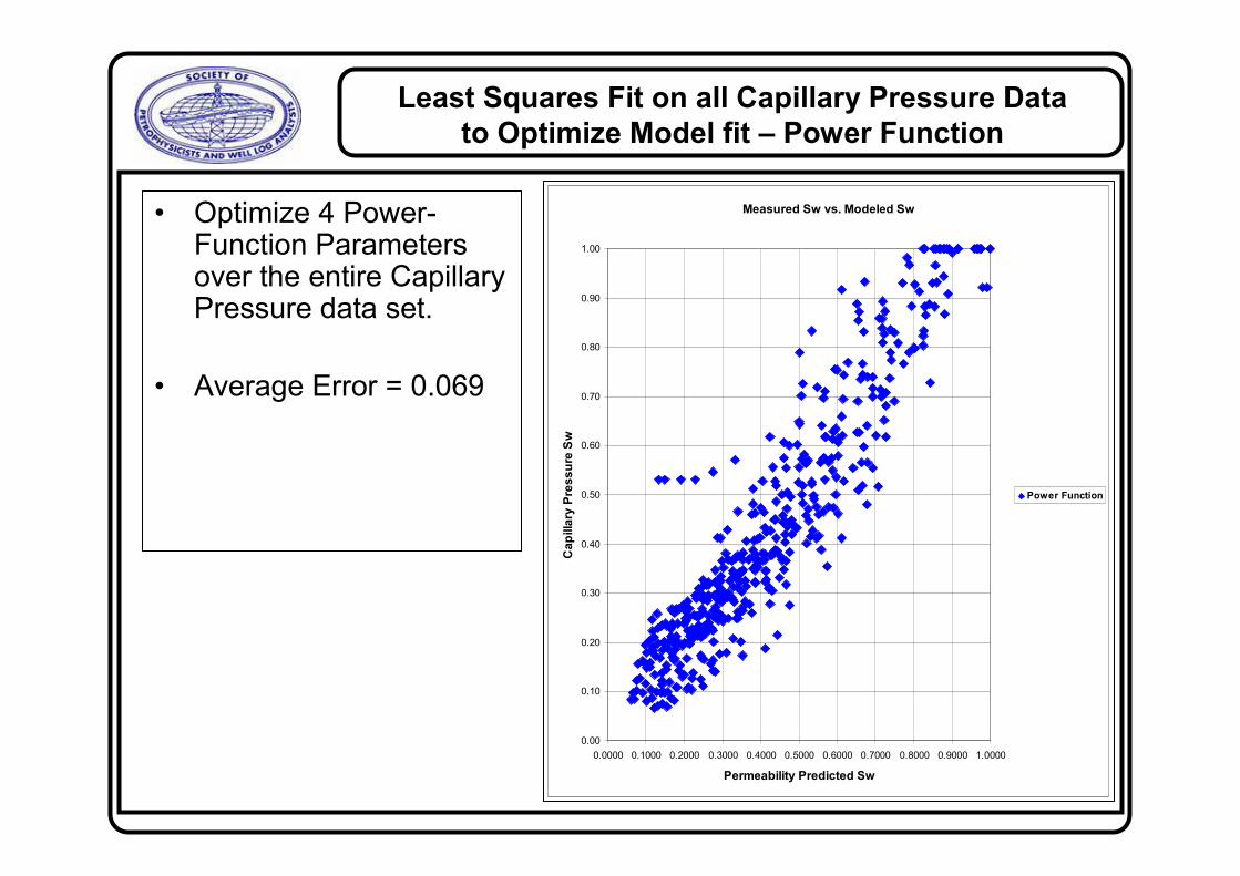
Least Squares Fit on all Capillary Pressure Data
to Optimize Model fit – Power Function
Measured Sw vs. Modeled Sw
0.00
0.10
0.20
0.30
0.40
0.50
0.60
0.70
0.80
0.90
1.00
0.0000 0.1000 0.2000 0.3000 0.4000 0.5000 0.6000 0.7000 0.8000 0.9000 1.0000
Permeability Predicted Sw
Capilla
ry P
ressure
Sw
Power Function
• Optimize 4 Power-Function Parameters over the entire Capillary Pressure data set.
• Average Error = 0.069
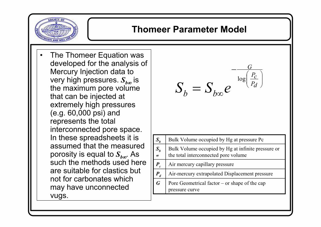
Thomeer Parameter Model
• The Thomeer Equation was developed for the analysis of Mercury Injection data to very high pressures. Sb∞∞∞∞ is the maximum pore volume that can be injected at extremely high pressures (e.g. 60,000 psi) and represents the total interconnected pore space. In these spreadsheets it is assumed that the measured porosity is equal to Sb∞∞∞∞. As such the methods used here are suitable for clastics but not for carbonates which may have unconnected vugs.
−
∞= dP
cP
G
eSS bb
log
Pore Geometrical factor – or shape of the cap
pressure curve
G
Air-mercury extrapolated Displacement pressurePd
Air mercury capillary pressurePc
Bulk Volume occupied by Hg at infinite pressure or
the total interconnected pore volume
Sb
∞∞∞∞
Bulk Volume occupied by Hg at pressure PcSb
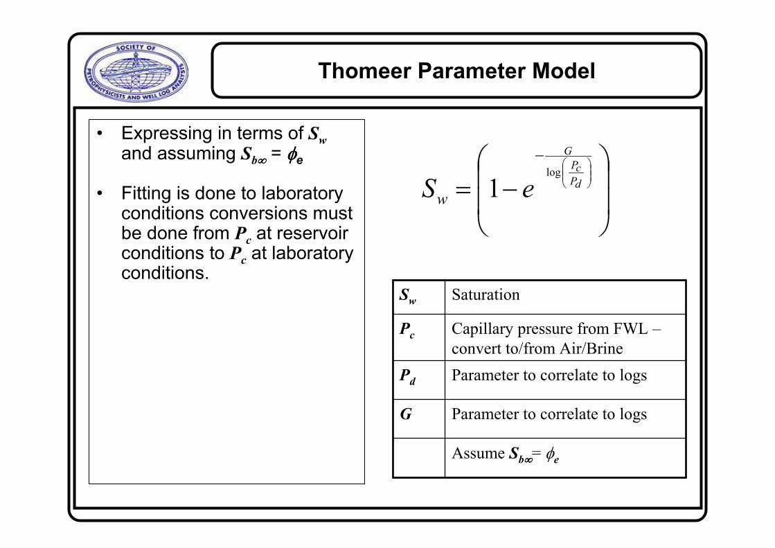
Thomeer Parameter Model
−=
−
dP
cP
G
eSwlog
1
• Expressing in terms of Sw
and assuming Sb∞∞∞∞ = φφφφe
• Fitting is done to laboratory conditions conversions must be done from Pc at reservoir conditions to Pc at laboratory conditions.
Assume Sb∞∞∞∞= φe
Parameter to correlate to logsG
Parameter to correlate to logsPd
Capillary pressure from FWL –
convert to/from Air/Brine
Pc
SaturationSw
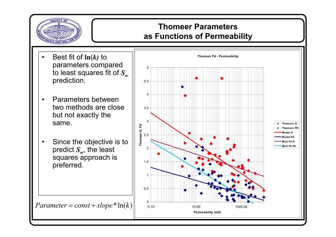
Thomeer Parameters
as Functions of Permeability
Thomeer Pd - Permeability
0
0.5
1
1.5
2
2.5
3
3.5
4
4.5
5
0.10 10.00 1000.00
Permeability (mD)
Thom
eer
G, P
d Thomeer G
Thomeer PD
Model G
Model Pd
Best Fit G
Best Fit Pd
)ln(* kslopeconstParameter +=
• Best fit of ln(k) to parameters compared to least squares fit of Sw
prediction.
• Parameters between two methods are close but not exactly the same.
• Since the objective is to predict Sw, the least squares approach is preferred.

Least Squares Fit on all Capillary Pressure Data
to Optimize Model fit – Thomeer Parameters
Measured Sw vs. Modeled Sw
0.00
0.10
0.20
0.30
0.40
0.50
0.60
0.70
0.80
0.90
1.00
0.0000 0.1000 0.2000 0.3000 0.4000 0.5000 0.6000 0.7000 0.8000 0.9000 1.0000
Permeability Predicted Sw
Capilla
ry P
ressure
Sw
Thomeer
• Optimize 4 J-Function Parameters over the entire Capillary Pressure data set.
• Average Error = 0.062
– Fitting error low in part due to limits put on computation at high permeabilies to remove irrational results.
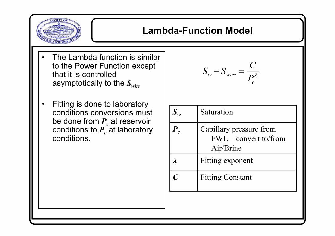
Lambda-Function Model
• The Lambda function is similar to the Power Function except that it is controlled asymptotically to the Swirr
• Fitting is done to laboratory conditions conversions must be done from Pc at reservoir conditions to Pc at laboratory conditions.
λc
wirrwP
CSS =−
Fitting ConstantC
Fitting exponentλλλλ
Capillary pressure from
FWL – convert to/from
Air/Brine
Pc
SaturationSw
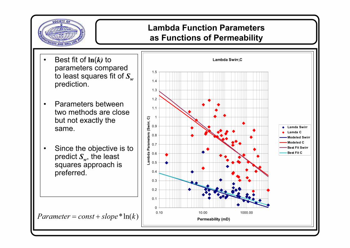
Lambda Function Parameters
as Functions of Permeability
Lambda Swirr,C
0
0.1
0.2
0.3
0.4
0.5
0.6
0.7
0.8
0.9
1
1.1
1.2
1.3
1.4
1.5
0.10 10.00 1000.00
Permeability (mD)
Lam
bda P
ara
mete
rs (Sw
irr, C
)
Lamda Swirr
Lamda C
Modeled Swirr
Modeled C
Best Fit Swirr
Best Fit C
)ln(* kslopeconstParameter +=
• Best fit of ln(k) to parameters compared to least squares fit of Sw
prediction.
• Parameters between two methods are close but not exactly the same.
• Since the objective is to predict Sw, the least squares approach is preferred.

Least Squares Fit on all Capillary Pressure Data
to Optimize Model fit – Lambda Function
Measured Sw vs. Modeled Sw
0.00
0.10
0.20
0.30
0.40
0.50
0.60
0.70
0.80
0.90
1.00
0.0000 0.1000 0.2000 0.3000 0.4000 0.5000 0.6000 0.7000 0.8000 0.9000 1.0000
Permeability Predicted Sw
Capilla
ry P
ressure
Sw
Lambda Function
• Optimize 5 Lambda Function Parameters over the entire Capillary Pressure data set.
• Average Error = 0.071
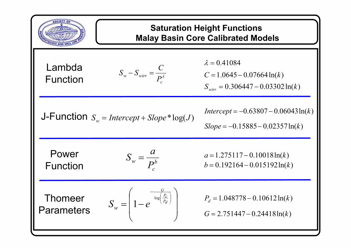
Saturation Height Functions
Malay Basin Core Calibrated Models
λc
wirrwP
CSS =−
)ln(03302.0306447.0 kSwirr −=
)ln(07664.00645.1 kC −=
41084.0=λ
)log(* JSlopeInterceptSw +=
b
c
wP
aS =
−=
−
dP
cP
G
eSwlog
1
)ln(06043.063807.0 kIntercept −−=
)ln(02357.015885.0 kSlope −−=
)ln(10018.0275117.1 ka −=)ln(015192.0192164.0 kb −=
)ln(10612.0048778.1 kPd −=
)ln(24418.0751447.2 kG −=
Lambda
Function
J-Function
Power
Function
Thomeer
Parameters
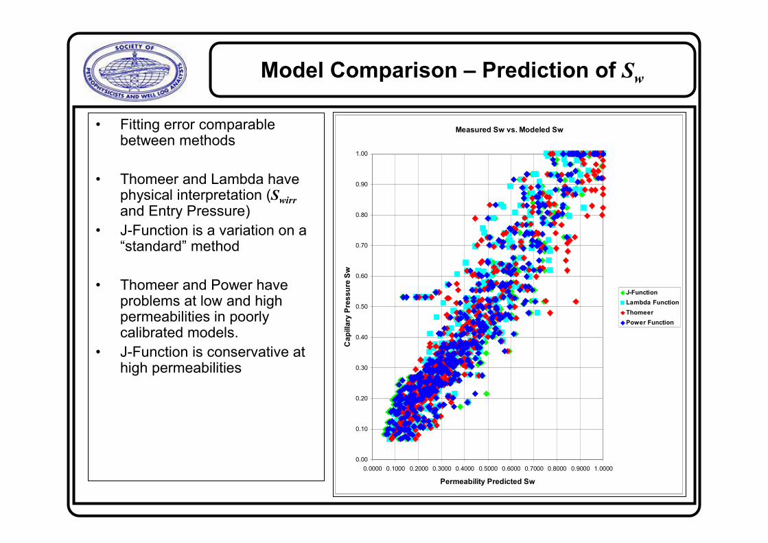
Model Comparison – Prediction of Sw
Measured Sw vs. Modeled Sw
0.00
0.10
0.20
0.30
0.40
0.50
0.60
0.70
0.80
0.90
1.00
0.0000 0.1000 0.2000 0.3000 0.4000 0.5000 0.6000 0.7000 0.8000 0.9000 1.0000
Permeability Predicted Sw
Capilla
ry P
ressure
Sw
J-Function
Lambda Function
Thomeer
Power Function
• Fitting error comparable between methods
• Thomeer and Lambda have physical interpretation (Swirrand Entry Pressure)
• J-Function is a variation on a “standard” method
• Thomeer and Power have problems at low and high permeabilities in poorly calibrated models.
• J-Function is conservative at high permeabilities
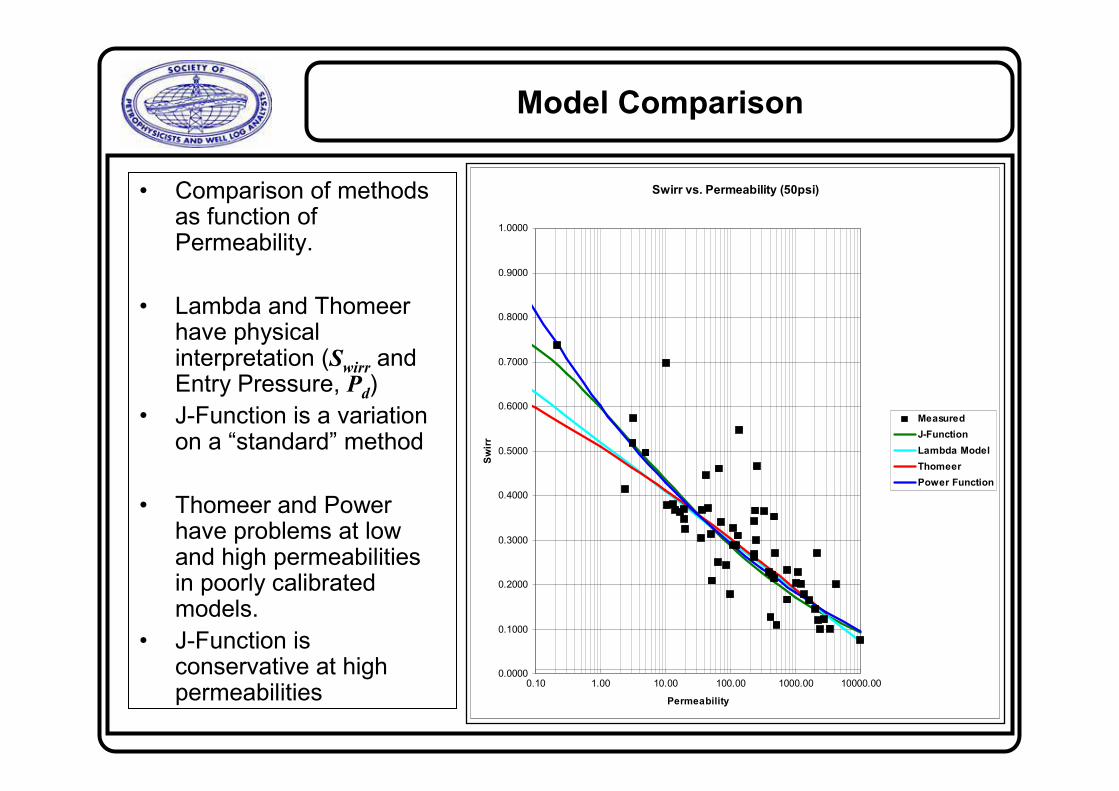
Model Comparison
Swirr vs. Permeability (50psi)
0.0000
0.1000
0.2000
0.3000
0.4000
0.5000
0.6000
0.7000
0.8000
0.9000
1.0000
0.10 1.00 10.00 100.00 1000.00 10000.00
Permeability
Sw
irr
Measured
J-Function
Lambda Model
Thomeer
Power Function
• Comparison of methods as function of Permeability.
• Lambda and Thomeer have physical interpretation (Swirr and Entry Pressure, Pd)
• J-Function is a variation on a “standard” method
• Thomeer and Power have problems at low and high permeabilities in poorly calibrated models.
• J-Function is conservative at high permeabilities

Example Comparing Different Methods.
2365
2370
2375
2385
2390
2395
2360
2380
2353.7
2400.0
2303.5
2310
2315
2320
2325
2330
2335
2340
2345.4

Clastic Permeability Review
• Permeability is a complex phenomena in rocks.
• Permeability is closely related to pore throat size.
• In clastics there is a loose relationship between pore throat size and grain size.
• There is a loose relationship between grain size and sorting.
• There is a loose relationship between porosity, sorting and grain size.
• Logs measure bulk properties and have little response to grain size and texture.
• These simplifications may be appropriate for clastics, but do not always work and are not necessarily applicable to carbonates or fractured reservoirs

(after Chilingar, 1969)(after Chilingar, 1969)
104
103
102
101
100
K in m
d
10-11
10-13
10-14
10-15
10-12
K in m
2
1 - coarse & very
coarse grained
2 - coarse & medium
coarse grained
3 - fine grained
4 - silty
5 - clayey
0 0.30.20.1 φ
Porosity - Permeability Relationships in Clastics
(Chilingar, 1969)(Chilingar, 1969)

(after Chilingar, 1969)(after Chilingar, 1969)
104
103
102
101
100
K in m
d
10-11
10-13
10-14
10-15
10-12
K in m
2
1 - coarse & very
coarse grained
2 - coarse & medium
coarse grained
3 - fine grained
4 - silty
5 - clayey
0 0.30.20.1 φ
Porosity - Permeability Relationships in Clastics
Observations
(Chilingar, 1969)(Chilingar, 1969)
Permeability decreases with decreasing
grain size.
Permeability increases with increasing
porosity.
Permeability does not increase infinitely
with porosity.
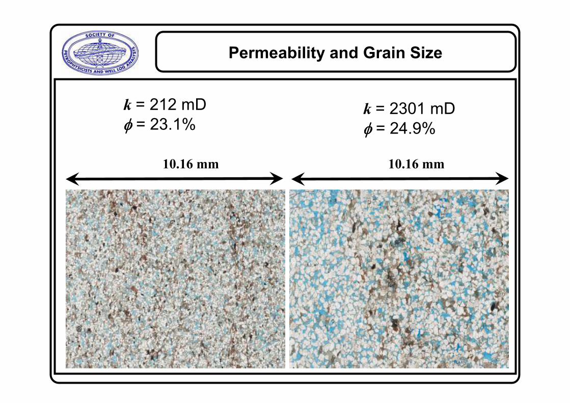
k = 2301 mD
φ φ φ φ = 24.9%
10.16 mm
Permeability and Grain Size
10.16 mm
k = 212 mD
φ φ φ φ = 23.1%

Common Permeability Models
2,4.4,136.0 === mnC
2,4,10 === mnC
Log - Fit
Timur
Coates
φbak +=10
m
wirr
n
SCk
φ=
m
e
e
n
e BVI
Ck
−
=φ
φφ*100
No standard values for the parameters. User derives parameters from
an appropriate fit of the core data.
Timur derived this equation in the 1960’s and assigned nominal
values. The user may adjust the fitting parameters to their data
Coates created this variation of the Timur equation, using
Bulk Volume of Immovable (BVI) fluid instead of Swirr for
use with NMR data. The model premise is that since
immovable water (Swirr) does not contribute to flow, there
should be a permeability control based on BVI.
Standard Values
Standard Values

Malay Basin Core Data – Log Fit
22 wells
Malay Basic Core Data
1 14
Color: FREQUENCY
0.000
0.050
0.100
0.150
0.200
0.250
0.300
0.350
0.400
0.01
0.1
1
10
100
1000
10000
100000
CORE.KAIR (MD)
CORE.PHI (V/V)
1091
9900
96
5 5
φ8.2170.210 +−=k
• Log-fit typical method often selected to “engineer” a good solution in a short period of time.
• Requires sufficient core for each reservoir or facies to be modeled to a desired accuracy.
• Simple (empirical) fits have minimal interpretive meaning.
• Single parameter input limits use when permeability is more complex.
• Tend to be limited to a certain porosity range.

Basic Inputs for Coates Equation
Well Sample Depth Lab Sigma Lab Theta Porosity Permeability Swirr C Lamda At 50 psi BVI Error
XXXXXX XXXX XXXX.XX 72 0 0.2160 46.00 0.21 0.78557 0.410837 0.371895 0.080329 0.2029
XXXXXX XXXX XXXX.XX 72 0 0.2180 136.00 0.46 0.525545 0.410837 0.560649 0.122222 0.2148
XXXXXX XXXX XXXX.XX 72 0 0.2030 86.00 0.13 0.75511 0.410837 0.278251 0.056485 0.2531
XXXXXX XXXX XXXX.XX 72 0 0.1800 14.40 0.17 0.830021 0.410837 0.336351 0.060543 0.3642
XXXXXX XXXX XXXX.XX 72 0 0.1090 3.26 0.40 0.798618 0.410837 0.556894 0.060701 0.3021
XXXXXX XXXX XXXX.XX 72 0 0.2390 238.00 0.18 0.378283 0.410837 0.253572 0.060604 0.1402
XXXXXX XXXX XXXX.XX 72 0 0.1840 13.20 0.20 0.81342 0.410837 0.364368 0.067044 0.3513
XXXXXX XXXX XXXX.XX 72 0 0.1850 20.30 0.15 0.850617 0.410837 0.319883 0.059178 0.2827
XXXXXX XXXX XXXX.XX 72 0 0.2290 249.00 0.22 0.388202 0.410837 0.299571 0.068602 0.1019
XXXXXX XXXX XXXX.XX 72 0 0.2150 111.00 0.18 0.562924 0.410837 0.287967 0.061913 0.1281
XXXXXX XXXX XXXX.XX 72 0 0.1900 35.70 0.17 0.788231 0.410837 0.332142 0.063107 0.3604
XXXXXX XXXX XXXX.XX 72 0 0.2560 439.00 0.16 0.341096 0.410837 0.224061 0.05736 0.1056
XXXXXX XXXX XXXX.XX 72 0 0.2550 1050.00 0.12 0.416837 0.410837 0.205739 0.052464 0.1133
XXXXXX XXXX XXXX.XX 72 0 0.2140 51.00 0.15 0.834018 0.410837 0.313839 0.067162 0.1713
XXXXXX XXXX XXXX.XX 72 0 0.2380 236.00 0.18 0.498915 0.410837 0.281581 0.067016 0.1592
XXXXXX XXXX XXXX.XX 72 0 0.2520 417.00 0.03 0.510268 0.410837 0.13486 0.033985 0.4942
XXXXXX XXXX XXXX.XX 72 0 0.2640 479.00 0.12 0.502782 0.410837 0.221984 0.058604 0.3755
XXXXXX XXXX XXXX.XX 72 0 0.1660 19.10 0.19 0.893739 0.410837 0.373563 0.062012 0.5065
XXXXXX XXXX XXXX.XX 72 0 0.2950 1360.00 0.11 0.298678 0.410837 0.16928 0.049937 0.1207
XXXXXX XXXX XXXX.XX 72 0 0.2810 2060.00 0.09 0.184025 0.410837 0.13183 0.037044 0.3138
XXXXXX XXXX XXXX.XX 72 0 0.1240 3.19 0.28 0.882574 0.410837 0.456714 0.056633 0.6406
XXXXXX XXXX XXXX.XX 72 0 0.1530 17.00 0.24 0.64846 0.410837 0.370708 0.056718 0.0850
XXXXXX XXXX XXXX.XX 72 0 0.1910 65.10 0.11 0.853812 0.410837 0.283332 0.054116 0.4561
XXXXXX XXXX XXXX.XX 72 0 0.1600 4.99 0.27 0.967255 0.410837 0.46705 0.074728 0.3846
XXXXXX XXXX XXXX.XX 72 0 0.2750 2740.00 0.05 0.403253 0.410837 0.134785 0.037066 0.1135
XXXXXX XXXX XXXX.XX 72 0 0.2170 493.00 0.20 0.301966 0.410837 0.261622 0.056772 0.2789
XXXXXX XXXX XXXX.XX 72 0 0.1430 65.90 0.31 0.576496 0.410837 0.422643 0.060438 0.5471
XXXXXX XXXX XXXX.XX 72 0 0.2560 1212.00 0.07 0.504979 0.410837 0.169278 0.043335 0.0618
XXXXXX XXXX XXXX.XX 72 0 0.2210 390.00 0.13 0.348139 0.410837 0.202318 0.044712 0.2650
XXXXXX XXXX XXXX.XX 72 0 0.2400 757.00 0.08 0.581892 0.410837 0.193623 0.046469 0.0493
XXXXXX XXXX XXXX.XX 72 0 0.2070 112.00 0.11 0.818213 0.410837 0.273856 0.056688 0.3220
XXXXXX XXXX XXXX.XX 72 0 0.2900 4213.00 0.08 0.446953 0.410837 0.170928 0.049569 0.1138
XXXXXX XXXX XXXX.XX 72 0 0.3090 2143.00 0.14 0.470232 0.410837 0.238535 0.073707 0.1351
XXXXXX XXXX XXXX.XX 72 0 0.2310 240.00 0.18 0.68961 0.410837 0.321134 0.074182 0.2138
Lambda Function Parameters

BVI from Capillary Pressure
• Capillary Pressure data can be
used to estimate BVI via Swirr
of the Lambda fitting.
Well XXXXXX
Fluids Air-Water
Method HS Centrifuge
NOB 800 psi
Klinkenberg Capillary End face
Sample Depth Permeability Porosity Pressure Sw
No. (m) (mD) (frac) (psi) (frac)
XXXX XXXX.XX 1050.00 0.2550 0.00 1.00
1.00 0.57
2.00 0.44
5.00 0.33
10.00 0.26
25.00 0.23
50.00 0.20
100.00 0.20
200.00 0.18
500.00 0.16
750.00 0.16
Air-Brine Capillary Pressure
0.00
100.00
200.00
300.00
400.00
500.00
600.00
700.00
800.00
0.00 0.20 0.40 0.60 0.80 1.00
Water Saturation
Air B
rine C
apilla
ry P
ressure
(Psi)
wirrSBVI φ=

Coates Equation Fit of Malay Basin Capillary
Pressure Data
Core Air Permeability - Modeled Pemeability
Capillary Pressure Data Only
0.10
1.00
10.00
100.00
1000.00
10000.00
0.1 1 10 100 1000 10000
Modeled Permeability
Core
Air P
erm
eability (m
D)
Coates
Unity
• Create Least squares fit of Capillary Pressure/Core Data (Swirr, φφφφ k) to Coates Parameters using capillary pressure 59 samples.
57.358.6036.0
23.9
*100
−
=e
eekφ
φφ

Coates: Permeability - Porosity
Capillary Pressure Data Only
0.10
1.00
10.00
100.00
1000.00
10000.00
0.0000 0.0500 0.1000 0.1500 0.2000 0.2500 0.3000 0.3500
Core Porosity
Core
Air
Perm
eability (m
D)
Poro-Perm
BVI=0.01
BVI=0.036
BVI=0.07
Coates Equation Fit of Malay Basin Capillary Pressure
• Fit of Coates model for BVI = 0.01, 0.036 and 0.07 for coarse grained, medium grained and fine grained (increasing surface to volume ratio resulting in increasing BVI.
• Model behaves as we would expect rocks to behave (i.e. decreasing permeability with increasing bound water.
• Similar behavior to known rock behavior

• Core calibrated Coates model with constant BVI of 0.01, 0.036 and 0.07.
• Coates model seeks to model permeability variations with grain-size though surface to volume relationships.
Core Calibrated Coates Model
18 WellsMalay Basin Core Data
Core Air Permeability vs. Core Porosity
1 12
Color: FREQUENCY
0.000
0.000
0.050
0.050
0.100
0.100
0.150
0.150
0.200
0.200
0.250
0.250
0.300
0.300
0.350
0.350
0.400
0.400
0.01 0.01
0.1 0.1
1 1
10 10
100 100
1000 1000
10000 1000020000 20000
Core Air Perm
eability (mD)
Core Porosity
943
8460
96
5 1

(after Chilingar, 1969)(after Chilingar, 1969)
104
103
102
101
100
K in m
d
10-11
10-13
10-14
10-15
10-12
K in m
2
1 - coarse & very
coarse grained
2 - coarse & medium
coarse grained
3 - fine grained
4 - silty
5 - clayey
0 0.30.20.1 φ
Permeability As a Function of
Porosity and Grain Size

• Core calibrated Coates model with constant BVI of 0.01, 0.036 and 0.07.
• Note how average BVI of 0.036 does not fit well over the entire range of porosity.
• This is because BVI changes with porosity (probably sorting of grains)
Core Calibrated Coates Model
18 WellsMalay Basin Core Data
Core Air Permeability vs. Core Porosity
1 12
Color: FREQUENCY
0.000
0.000
0.050
0.050
0.100
0.100
0.150
0.150
0.200
0.200
0.250
0.250
0.300
0.300
0.350
0.350
0.400
0.400
0.01 0.01
0.1 0.1
1 1
10 10
100 100
1000 1000
10000 1000020000 20000
Core Air Perm
eability (mD)
Core Porosity
943
8460
96
5 1

Capilliary Pressure BVI vs. Core Porosity
0.0000
0.0200
0.0400
0.0600
0.0800
0.1000
0.1200
0.1400
0.00 0.05 0.10 0.15 0.20 0.25 0.30 0.35 0.40 0.45
Core Porosity
Capilliary
Pre
ssure
BV
I
BVI
Fit
• Simple model of BVI vs. φφφφ to capture variable of BVI due to rock quality.
φφ
≤≤
−=
BVI
BVI
01.0
29.010.0
Variation of BVI with Porosity

φφ
≤≤
−=
BVI
BVI
01.0
29.010.0
• Final Coates Model with variable BVI achieves better fit with all the core data.
• Honors core calibration parameters.
• If BVI data is available from NMR or other sources it may be used in place of the Simple BVI to φφφφrelationship.
57.358.6
23.9
*100
−
=e
ee BVIk
φφφ
Core Calibrated Coates Model with Variable
BVM – Generic Malay Basin Model
18 WellsMalay Basin Core Data
Core Air Permeability vs. Core Porosity
1 12
Color: FREQUENCY
0.000
0.000
0.050
0.050
0.100
0.100
0.150
0.150
0.200
0.200
0.250
0.250
0.300
0.300
0.350
0.350
0.400
0.400
0.01 0.01
0.1 0.1
1 1
10 10
100 100
1000 1000
10000 1000020000 20000
Core Air Perm
eability (mD)
Core Porosity
943
8460
96
5 1
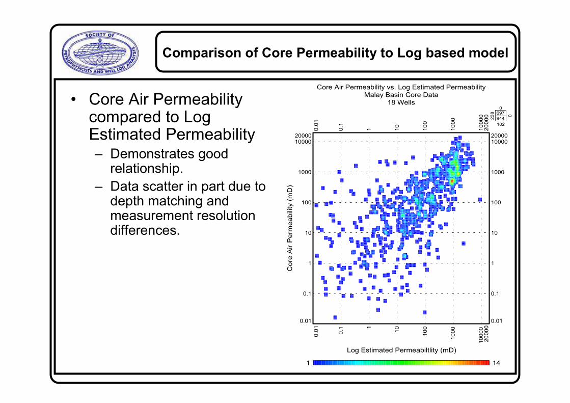
• Core Air Permeability compared to Log Estimated Permeability– Demonstrates good
relationship.
– Data scatter in part due to depth matching and measurement resolution differences.
Comparison of Core Permeability to Log based model
18 WellsMalay Basin Core Data
Core Air Permeability vs. Log Estimated Permeability
1 14
0.01
0.01
0.1
0.1
11
10
10
100
100
1000
1000
10000
10000
20000
20000
0.01 0.01
0.1 0.1
1 1
10 10
100 100
1000 1000
10000 1000020000 20000
Core Air Perm
eability (mD)
Log Estimated Permeabiltlity (mD)
944
6970
102
238
0

Pore Volume Definition Review
Bulk Volume MovableBVM
Bound Water Irreducible – also known as Capillary bound
Water
BVI
Clay Bound Water – water hydrated on clay surface.CBW
Effective Porosityφφφφe
Total Porosityφφφφt
φφφφeVq Vsh
Silt
Clay Bound W
ater
Bulk Volume
Movable (BVM)
Capillary Bound
Water (B
VI)BVIBVM
CBW
e
et
+=
+=
φ
φφ
Humidity dried core is expected to relate to
Effective Porosity, φe, since humidity drying
cannot remove the Clay Bound Water.
When relating to logs and log derived effective
porosity there are some differences which
become more pronounced as shaliness
increases because log analysis tends to define
capillary bound water in shale as CBW. While it
is non-effective, technically it is not the water of
hydration.
Clay

MatrixMatrixDryDryClayClay
Clay-Clay-BoundBoundWaterWater
MobileMobileWaterWater
CapillaryCapillaryBoundBoundWaterWater
HydrocarbonHydrocarbon
Echo A
mplitu
de
0 15 1501351201059075604530
Time (ms)
20
15
10
5
T2 Decay
NMR Porosity
Transform
0.00
1.00
2.00
3.00
4.00
0.1 1 10 100 1000 10000
BVI BVM
4.00
0.00
1.00
2.00
3.00
Incre
menta
l P
oro
sity (pu)
CBW
T2 Decay (ms)
T2 Cutoffs
ECHO TRAIN T2 SPECTRUM
25
NMR Basics

0
1
2
3
4
5
6
0 10 20 30 40 50 60 70 80 90 100
Water Saturation, % pore volume
Pressure, bar
Simple (Undisturbed) Reservoir States
Above the transition zone, pressure difference due to the density difference
between hydrocarbon and water force water to drain from the reservoir. This
volume of hydrocarbon can be approximated by Swirr or BVI
Silt
Clay Bound
Water
Hydrocarbon
Capillary Bound
Water (BVI)
Clay
Silt
Clay Bound
Water
Transition
Capillary Bound
Water (BVI)
Clay
Silt
Clay Bound
Water
Wet
Capillary Bound
Water (BVI)
Clay
Within the transition zone pressure is insufficient to displace all the water and
“free” water may be produced. The length of the transition zone is determined by
the fluid density differences and the capillary properties. In general high
permeability means short transition zones.
Below the OWC the formation is 100% wet.
Rule of “Thumb” reservoir
is either “wet” or near Swirr.

I-Gas Sand Analysis using Generic Models
2080
2085
2090
2095
2105
2110
2115
2120
2130
2135
2140
2145
2100
2125
2050
2055
2060
2065
2070
2075
2080
2085
2090
2095
2100
2105
2110
2115
I8014.9
2090.9I90
2093.1
I90 SAND25.9
2119.0
I90 SHALE13.1
2132.1
I10025.0
I8014.9
2090.9I90
2093.1
I90 SAND25.9
2119.0
I90 SHALE13.1
2132.1
I10025.0

2080
2085
2090
2095
2105
2110
2115
2120
2130
2135
2140
2145
2100
2125
2050
2055
2060
2065
2070
2075
2080
2085
2090
2095
2100
2105
2110
2115
I8014.9
2090.9I90
2093.1
I90 SAND25.9
2119.0
I90 SHALE13.1
2132.1
I10025.0
I8014.9
2090.9I90
2093.1
I90 SAND25.9
2119.0
I90 SHALE13.1
2132.1
I10025.0
I-Gas Sand with NMR data
2330
2335
2340
2345
2355
2360
2365
2370
2380
2385
2390
2395
2405
2410
2415
2420
2430
2435
2350
2375
2400
2425
2280
2285
2290
2295
2300
2305
2310
2315
2320
2325
2330
2335
2340
2345
2350
2355
2360
2365
2370
2375
2380
2331.7
J509.1
2340.9
J50 SHALE12.8
2353.7
J5518.6
2372.3
J6027.7
2400.0
J7023.2
2423.2
K520.1
2331.7
J509.1
2340.9
J50 SHALE12.8
2353.7
J5518.6
2372.3
J6027.7
2400.0
J7023.2
2423.2
K520.1
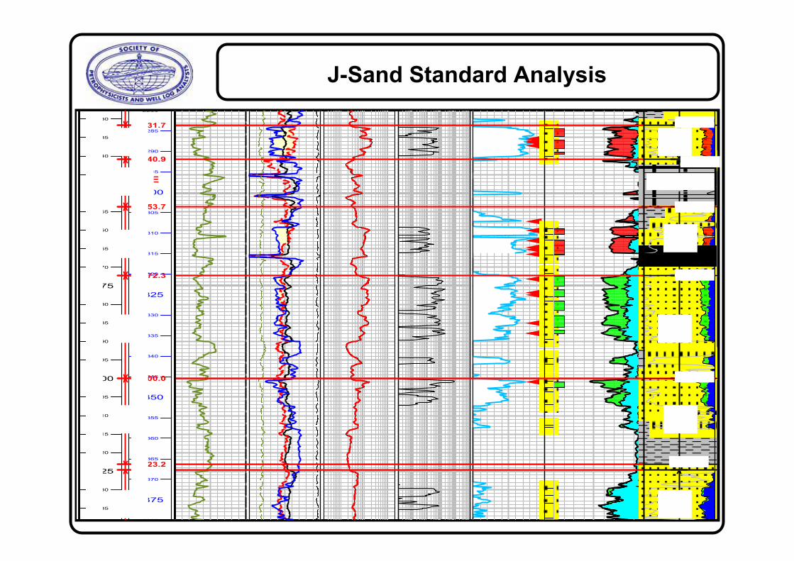
J-Sand Standard Analysis
2330
2335
2340
2345
2355
2360
2365
2370
2380
2385
2390
2395
2405
2410
2415
2420
2430
2435
2350
2375
2400
2425
2280
2285
2290
2295
2300
2305
2310
2315
2320
2325
2330
2335
2340
2345
2350
2355
2360
2365
2370
2375
2380
2331.7
J509.1
2340.9
J50 SHALE12.8
2353.7
J5518.6
2372.3
J6027.7
2400.0
J7023.2
2423.2
K520.1
2331.7
J509.1
2340.9
J50 SHALE12.8
2353.7
J5518.6
2372.3
J6027.7
2400.0
J7023.2
2423.2
K520.1
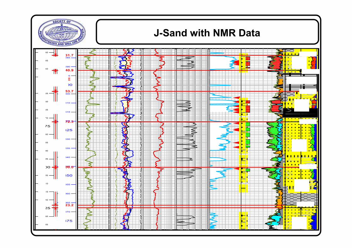
J-Sand with NMR Data

2330
2335
2340
2345
2355
2360
2365
2370
2380
2385
2390
2395
2405
2410
2415
2420
2430
2435
2350
2375
2400
2425
2280
2285
2290
2295
2300
2305
2310
2315
2320
2325
2330
2335
2340
2345
2350
2355
2360
2365
2370
2375
2380
2331.7
J509.1
2340.9
J50 SHALE12.8
2353.7
J5518.6
2372.3
J6027.7
2400.0
J7023.2
2423.2
K520.1
2331.7
J509.1
2340.9
J50 SHALE12.8
2353.7
J5518.6
2372.3
J6027.7
2400.0
J7023.2
2423.2
K520.1
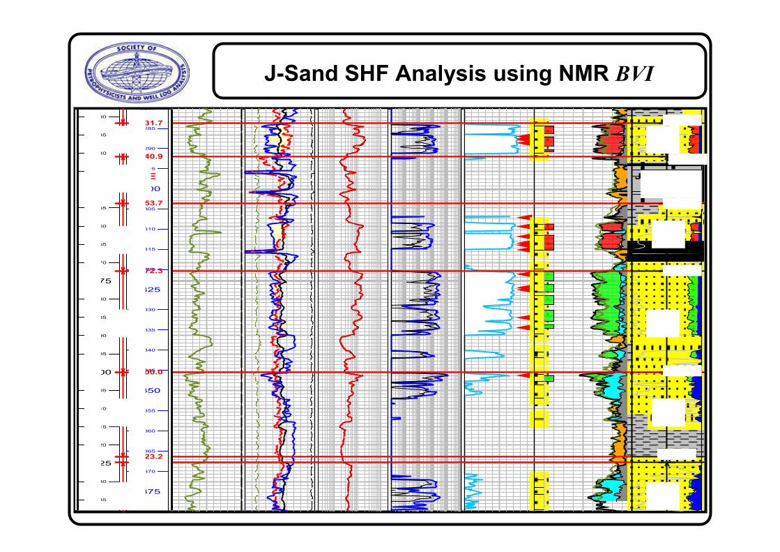
J-Sand SHF Analysis
2330
2335
2340
2345
2355
2360
2365
2370
2380
2385
2390
2395
2405
2410
2415
2420
2430
2435
2350
2375
2400
2425
2280
2285
2290
2295
2300
2305
2310
2315
2320
2325
2330
2335
2340
2345
2350
2355
2360
2365
2370
2375
2380
2331.7
J509.1
2340.9
J50 SHALE12.8
2353.7
J5518.6
2372.3
J6027.7
2400.0
J7023.2
2423.2
K520.1
2331.7
J509.1
2340.9
J50 SHALE12.8
2353.7
J5518.6
2372.3
J6027.7
2400.0
J7023.2
2423.2
K520.1
J-Sand SHF Analysis using NMR BVI
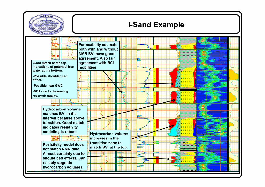
I-Sand Example
Permeability estimate
both with and without
NMR BVI have good
agreement. Also fair
agreement with RCI
mobilities
Hydrocarbon volume
increases in the
transition zone to
match BVI at the top.
Hydrocarbon volume
matches BVI in the
interval because above
transition. Good match
indicates resistivity
modeling is robust
Good match at the top.
Indications of potential free
water at the bottom.
-Possible shoulder bed
effect.
-Possible near GWC
-NOT due to decreasing
reservoir quality.
Resistivity model does
not match NMR data.
Almost certainly due to
should bed effects. Can
reliably upgrade
hydrocarbon volumes.
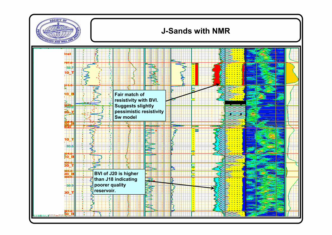
J-Sands with NMR
Fair match of
resistivity with BVI.
Suggests slightly
pessimistic resistivity
Sw model
BVI of J20 is higher
than J18 indicating
poorer quality
reservoir.
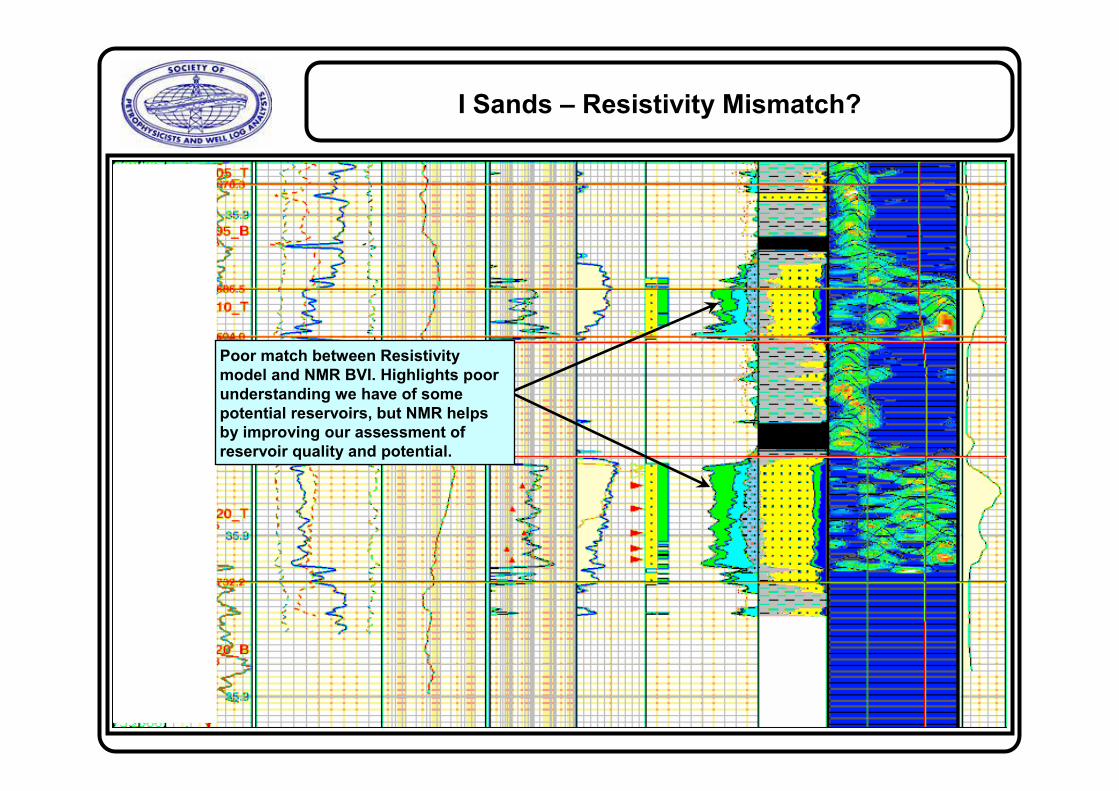
I Sands – Resistivity Mismatch?
Poor match between Resistivity
model and NMR BVI. Highlights poor
understanding we have of some
potential reservoirs, but NMR helps
by improving our assessment of
reservoir quality and potential.
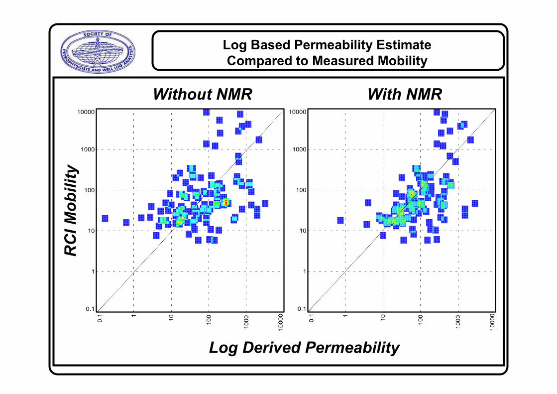
Log Based Permeability Estimate
Compared to Measured Mobility
0.1 1
10
100
1000
10000
0.1
1
10
100
1000
10000
0.1 1
10
100
1000
10000
0.1
1
10
100
1000
10000
Without NMR With NMR
Log Derived Permeability
RCI Mobility
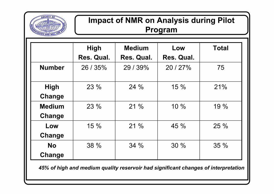
Impact of NMR on Analysis during Pilot
Program
35 %30 %34 %38 %No
Change
25 %45 %21 %15 %Low
Change
19 %10 %21 %23 %Medium
Change
21%15 %24 %23 %High
Change
7520 / 27%29 / 39%26 / 35%Number
TotalLow
Res. Qual.
Medium
Res. Qual.
High
Res. Qual.
45% of high and medium quality reservoir had significant changes of interpretation
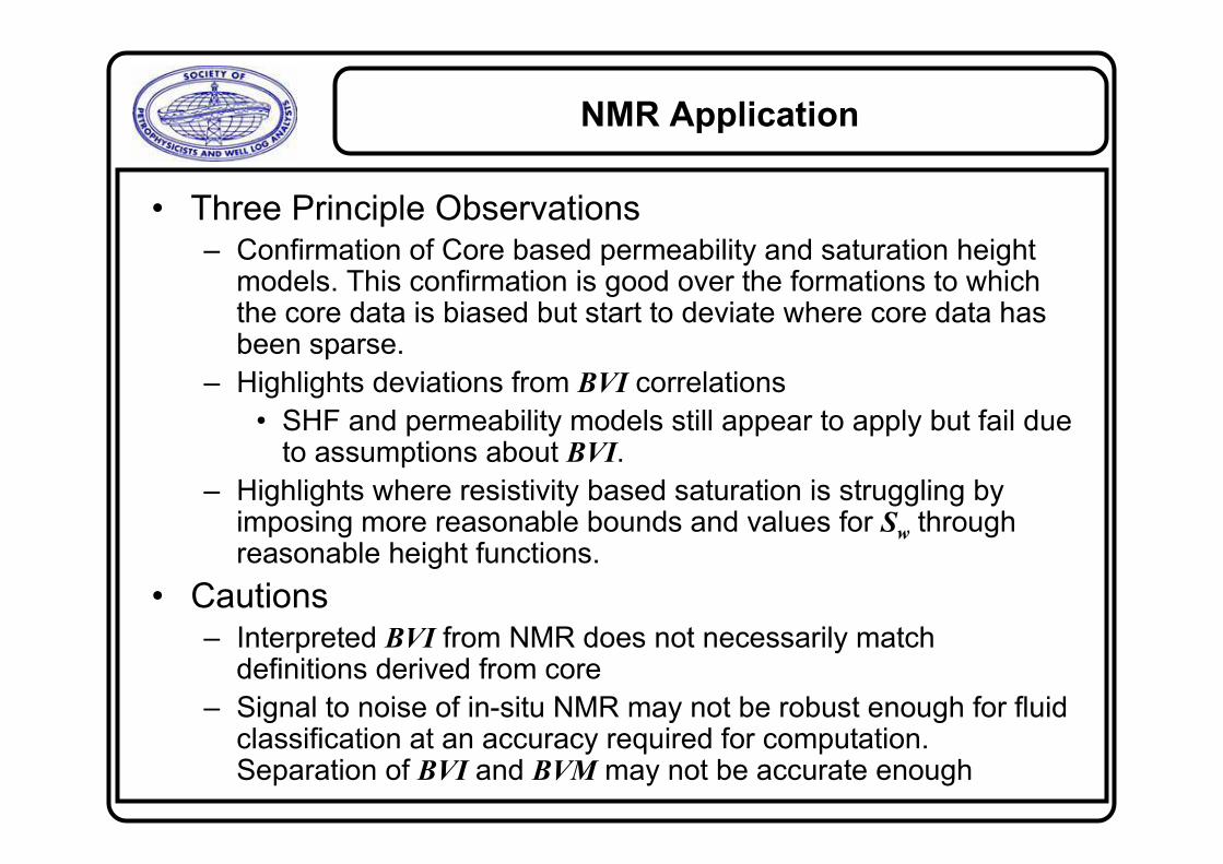
NMR Application
• Three Principle Observations– Confirmation of Core based permeability and saturation height
models. This confirmation is good over the formations to which the core data is biased but start to deviate where core data hasbeen sparse.
– Highlights deviations from BVI correlations
• SHF and permeability models still appear to apply but fail due to assumptions about BVI.
– Highlights where resistivity based saturation is struggling by imposing more reasonable bounds and values for Sw through reasonable height functions.
• Cautions– Interpreted BVI from NMR does not necessarily match
definitions derived from core
– Signal to noise of in-situ NMR may not be robust enough for fluid classification at an accuracy required for computation. Separation of BVI and BVM may not be accurate enough

Conclusions
• Several different Saturation Height functions give similar results when implemented as correlations to permeability– Use which ever model you feel comfortable with or that fits your
modeling work flow.
• Capillary pressure may be used to derive the parameters of the Coates equation providing a non-log and non-NMR method of verifying/calibrating the Coates permeability model.
• Used appropriately, NMR BVI measurements are compatible with the methods above and provide guidance on permeability and saturation.– Caution must be exercised in the interpretation of the NMR data.
• Using these methods, log derived permeability achieves greater consistency with mobility from pressure measurements.
Acknowledgements
PVEP
For permission to present the data
and results I would like to thank:
PETRONAS
PETRONAS – Carigali
Petro-Vietnam Production Corporation


![RENAULT TALISMAN [2016+] 31110 RENAULT TALISMAN … · 31110 1.0 28/09/2018 2 31110 renault talisman renault talisman grandtour [2016+] [2016+] type rfd kg s = 100 e3 55r-01 7907](https://static.fdocuments.in/doc/165x107/5ed0802b8862292f7d0cdc2a/renault-talisman-2016-31110-renault-talisman-31110-10-28092018-2-31110-renault.jpg)


![INDEX: The Cape Malay/Muslim Dictionary (words with ... · PDF fileAjoemat - (talisman/amulet) [azeemah mispronounced] Akeltjies - (additional turns and twists added while pitching](https://static.fdocuments.in/doc/165x107/5aaec0f07f8b9a190d8c7f61/index-the-cape-malaymuslim-dictionary-words-with-talismanamulet-azeemah.jpg)


