Taking Time Seriously: Dynamic Regression

August 15, 2006

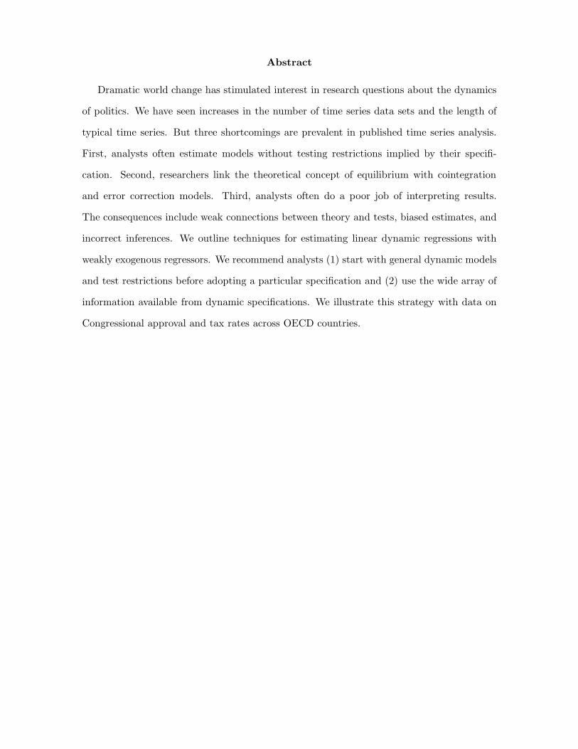
Abstract

Dramatic world change has stimulated interest in research questions about the dynamics

of politics. We have seen increases in the number of time series data sets and the length of

typical time series. But three shortcomings are prevalent in published time series analysis.

First, analysts often estimate models without testing restrictions implied by their specifi-

cation. Second, researchers link the theoretical concept of equilibrium with cointegration

and error correction models. Third, analysts often do a poor job of interpreting results.

The consequences include weak connections between theory and tests, biased estimates, and

incorrect inferences. We outline techniques for estimating linear dynamic regressions with

weakly exogenous regressors. We recommend analysts (1) start with general dynamic models

and test restrictions before adopting a particular specification and (2) use the wide array of

information available from dynamic specifications. We illustrate this strategy with data on

Congressional approval and tax rates across OECD countries.

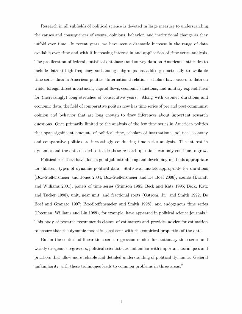
Research in all subfields of political science is devoted in large measure to understanding

the causes and consequences of events, opinions, behavior, and institutional change as they

unfold over time. In recent years, we have seen a dramatic increase in the range of data

available over time and with it increasing interest in and application of time series analysis.

The proliferation of federal statistical databases and survey data on Americans’ attitudes to

include data at high frequency and among subgroups has added geometrically to available

time series data in American politics. International relations scholars have access to data on

trade, foreign direct investment, capital flows, economic sanctions, and military expenditures

for (increasingly) long stretches of consecutive years. Along with cabinet durations and

economic data, the field of comparative politics now has time series of pre and post communist

opinion and behavior that are long enough to draw inferences about important research

questions. Once primarily limited to the analysis of the few time series in American politics

that span significant amounts of political time, scholars of international political economy

and comparative politics are increasingly conducting time series analysis. The interest in

dynamics and the data needed to tackle these research questions can only continue to grow.

Political scientists have done a good job introducing and developing methods appropriate

for different types of dynamic political data. Statistical models appropriate for durations

(Box-Steffensmeier and Jones 2004; Box-Steffensmeier and De Boef 2006), counts (Brandt

and Williams 2001), panels of time series (Stimson 1985; Beck and Katz 1995; Beck, Katz

and Tucker 1998), unit, near unit, and fractional roots (Ostrom, Jr. and Smith 1992; De

Boef and Granato 1997; Box-Steffensmeier and Smith 1998), and endogenous time series

(Freeman, Williams and Lin 1989), for example, have appeared in political science journals.1

This body of research recommends classes of estimators and provides advice for estimation

to ensure that the dynamic model is consistent with the empirical properties of the data.

But in the context of linear time series regression models for stationary time series and

weakly exogenous regressors, political scientists are unfamiliar with important techniques and

practices that allow more reliable and detailed understanding of political dynamics. General

unfamiliarity with these techniques leads to common problems in three areas:2

1

• First, analysts tend to adopt restrictive dynamic specifications on the basis of limited

theoretical guidance and without empirical evidence that restrictions are valid, poten-

tially biasing inferences and invalidating hypothesis tests.3

• Second, political scientists have linked the theoretical concept of equilibrium with the

existence of cointegration and use of error correction models. As a result, analysts

don’t typically derive equilibrium conditions, estimate error correction rates, or use error

correction models unless the data are found to be cointegrated. But, (1) error correction

models represent a general class of regression models appropriate for stationary data and

(2) all regressions describe equilibrium conditions and error correction rates. Exclusively

linking error correction models to cointegration limits our ability to use them effectively

to understand the dynamics of politics.

• Third and finally, once analysts select and estimate a model, inferences are typically

limited to short-run effects and interpretation follows that of a static model: “a unit

change in X (at t− s) leads to an expected change in Y (at time t)”. As such, analysts

frequently fail to compute and interpret quantities such as long run impacts of exogenous

variables, mean and median lag lengths of effects, equilibrium conditions, and the rate

of equilibrium correction. These quantities allow for statistical tests of the relevant

theoretical model, and without them, the inferences we draw are incomplete.

Until we solve these problems, political theory and hypotheses will be under-tested and

our understanding of the temporal nature of politics incomplete. Here, we focus on the tech-

niques needed to use dynamic regression models effectively. Specifically, we: (1) recommend

researchers begin time series analysis with the estimation of a general time series model

(guided by theory) and test restrictions on that model, (2) demonstrate that error correction

models are suitable for stationary data, (3) provide details on how to interpret a variety of

quantities of interest from dynamic regression models that are seldom presented in applied

work but that are informative theoretically, and (4) we use empirical examples to illustrate

the difference that good specification and interpretation can make for the kinds of inferences

we draw about the dynamics of politics. The techniques we present apply to time series cross

section data as well.

2

While others have visited some of these topics before, previous work does not provide

systematic coverage of the necessary techniques. For example, there has been some presen-

tation of various dynamic models and their interpretation (Beck 1985, 1991), but without

attention to general-to-specific modeling techniques. And others have debated the nature of

error correction models (Beck 1992; Durr 1992a,b), but provided no definitive resolution to

how and when they can be used. Moreover, as we will demonstrate, what coverage there has

been has been largely ignored.

Careful time series analysis is a critical part of the study of change and its consequences.

Estimating restricted models, misunderstanding equilibria, and poor interpretation under-

mine careful analysis. They lead, at best, to weakly connected theory and tests and a limited

cumulation of knowledge. Too often the costs include biased results and incorrect inferences

as well. The recommendations that follow help analysts avoid these costs and are central to

good time series practice.

Time Series Models in the Literature

We claim that being unaware of several time series techniques, analysts routinely make three

mistakes: (1) they adopt restrictive specifications without evidence that restrictions are valid;

(2) they link the theoretical concept of equilibrium with the existence of cointegration and

use of error correction models (ECMs) and therefore do not derive equilibrium conditions,

estimate error correction rates, or use error correction models unless the data are found to be

cointegrated; and (3) they draw limited inferences about theoretical quantities of interest due

to poor interpretation of dynamic models. To provide evidence for this claim, we searched

articles appearing in The American Political Science Review, The American Journal of Po-

litical Science, and The Journal of Politics between 1995 and 2005, cataloging the types of

dynamic analysis conducted, the models specified, the theoretical and statistical evidence

presented for the specification, and the nature of interpretation of the results.

Between 1995 and 2005 73 articles were published using time series regression techniques

in the context of stationary data. Of these only 10 either started with a general model

or tested whether restrictions were empirically valid. Of these 10, only 4 expressly began

with a general model; more than 85% of the articles examined did not test whether the

3

restrictions used were empirically valid. Our review suggests not only that restrictive models

are prevalent, but also that dynamic specifications are often selected ad hoc. In particular,

frequently there is neither a discussion of the decision to include contemporaneous values of

the exogenous variables as opposed to (or in addition to) lagged values nor is there a report

of lag lengths tests. In fact, no article reported tests for lag lengths.

Authors can be rather cavalier about how they deal with serial correlation. Two manuscripts

that estimated static regressions did not discuss this specification choice at all. In one piece,

the decision to include a lagged dependent variable was relegated to a footnote and the esti-

mated coefficient and standard error were not reported. And the most common restriction

imposed—restricting contemporaneous effects of the independent variables to be zero—is

often not discussed at all. Quite often this specification or one with a lagged dependent

variable is simply used as an afterthought to cure serial correlation.

The estimation of restricted models in and of itself is not evidence of poor specification.

Combined with the lack of evidence for the validity of restrictions and justification for the

specifications estimated, however, it suggests a potential for bias. The regularity with which

we see this pattern of results is disturbing. It suggests that analysts are either unaware of op-

tions within the class of general time series regression specifications, ways to test restrictions

on these specifications, or the consequences of estimating overly restrictive models.

The misunderstanding over error correction models is more likely to manifest itself in the

form of omission in the context of stationary time series. That is, since most analysts have

stationary data and associate error correction with cointegration, they won’t use an ECM.

This appears to be the case: of the 73 articles that used dynamic regression only 8 used

ECMs, and only two understood that cointegration is not necessary to justify their use. We

presume that other pieces might have relied upon ECMs if they were better understood.

Last, we examined how many authors did more than interpret the estimated results as

static effects. Here, the results are slightly better, but outside the context of ECMs, where

equilibrium correction rates and long run effects are typically interpreted, only 26% of the

65 articles examined provided any interpretation of dynamic quantities. That is, well over

a majority of the articles we examined treated dynamic quantities as static. Our review of

the literature demonstrates that these errors are not isolated. In the top journals of the

4

discipline, analysts regularly misuse dynamic specification. We next examine in more detail

why such errors matter and outline proofs and techniques to help analysts avoid them.4

General Models and Perils of Neglecting Them

In this section, we present a general model from econometrics for the estimation of dynamic

time series regressions for stationary data with (at least) weakly exogenous regressors. This

model should be the starting point for all time series regression. We discuss its importance for

developing good specifications, show how restricting the model leads to other specifications,

and demonstrate how invalid restrictions lead to biased inferences.

A General Model

Theories about politics typically tell us only generally how inputs relate to political processes

we care about. They are nearly always silent on which lags matter, whether levels or changes

drive Yt, what characterizes equilibrium behavior, or what effects are likely to be biggest in

the long run. Occasionally theory tells us Xt affects Yt with a distributed lag. Literature

on the relationship between public opinion and Supreme Court decisions is typical. Mishler

and Sheehan (1996) write: “Although each hypothesis predicts a lag in the impact of public

opinion on judicial decisions, none is sufficiently developed in theory to specify the precise

length of the expected lag.” Mondak and Smithey develop a detailed model specifically

to predict and identify reasonable equilibrium behavior for support for the Court but are

agnostic about the specific dynamics (Mondak and Smithey 1997). The story is the same in

other fields; theory tells us only generally that the (current and) past matters; it is mute on

the specifics of specification.

Substantive theory, then, typically does not provide enough guidance for precise dynamic

specifications. Econometric theory is clear in this case: analysts should start with a general

model—one that subsumes the data generating process (Hendry 1995). Only then should

we test restrictions, the inclusion of particular Xt (and Yt) as well as lags. In the context of

stationary data and weakly exogenous regressors, the following model fits our criteria5:

Yt = α0 +

p∑

i=1

αiYt−i +

n∑

j=1

q∑

i=0

βjpXjt−i + εt (1)

5

where εt is white noise, |∑p

i=1 αi| < 1 so that Yt is stationary, and the processes generating

Xj are weakly exogenous for the parameters of interest such that E(εt,Xjs) = 0∀ t, s, and j.

This is an autoregressive distributed lag or ADL(p, q;n) model, where p refers to the number

of lags of Yt, q the number of lags of Xt, and n the number of exogenous regressors.6

Such a general model has much to recommend it. In particular, it makes no assumptions

about the lags at which Xt influences Yt. Further, it should be consistently estimated by or-

dinary least squares (OLS) (Davidson and MacKinnon 1993).7 Finally, the model nests many

commonly estimated specifications and therefore can be used to test the appropriateness of

the restrictions those models imply on the general ADL.

For simplicity, we refer to the case when p = q = n = 1, but the results generalize:8

Yt = α0 + α1Yt−1 + β0Xt + β1Xt−1 + εt. (2)

The estimated coefficients, β0 and β1, called short run or impact multipliers, give the imme-

diate effect on Yt of a unit change in Xt at a given t. If Xt is a measure of economic ex-

pectations and data are quarterly, β0 tells us how levels of economic expectations in 1991Q2

affect presidential approval in that same quarter. β1 tells us how previous levels of economic

expectations in 1991Q1 affect presidential approval in the subsequent quarter. The long run

effect, referred to as the long run, dynamic, or total multiplier, is given by k1 = (β0+β1)(1−α1) .

The ADL is a fully general dynamic model and a number of more familiar models are a

special case of the ADL. Table 1 lists statistical models that are special cases of the ADL

and the restrictions each imposes. All of these models result from imposing restrictions on

the parameters of the ADL, each of which can be tested in the context of the ADL using

t-tests or F-tests. For example, to determine whether the partial adjustment model (PA) is

consistent with the DGP, we estimate the ADL and conduct a t-test on β1 = 0. If we cannot

reject the null, then we can proceed to draw inferences from the PA model assured that the

restriction is valid. If we reject the null, then we need to either test alternate restrictions or

proceed with an analysis of the general model.

Insert Table 1 about here.

6

The Costs of Invalid Restrictions

What happens when analysts impose invalid restrictions? That is, what happens when

analysts estimate a restricted model when a more general or alternative form is appropriate?

Consider the common practice of restricting β1 = 0. Analysts should only impose this re-

striction after testing its validity. The resulting PA model is, however, often estimated based

only on an appeal to a broad theoretical justification that is necessary, but not sufficient,

for a PA model: the effects of X are biggest in the current period and decay in subsequent

periods. Occasionally, a more specific theoretical story is offered: individuals or governments

pursue target values of Yt given current values of Xt, but changing Yt is costly so that im-

mediate adjustment—change—in Yt is slow or partial.9 Nadeau et al. are unique in offering

a theoretical justification for their empirical specification of models of presidential approval,

economic forecasts, and economic attitudes, writing: “From a theoretical perspective, the

‘partial adjustment’ model...guided our model specification since individuals, whether they

are masses or elites, adjust incompletely to new information that becomes available in a

given period. This incomplete adjustment could be due to psychological or institutional con-

straints.” (Nadeau et al. 1999, 130). More typically, however, the justification doesn’t appeal

to theory at all, as the lagged dependent variable is included to clean up serial correlation.

When this restriction is invalid, β0 and α1 will be biased. The degree and direction of bias

are a function of the covariance of Xt and Yt−1, respectively, with Xt−1. Because Xt tends

to be highly autocorrelated, the bias in β0 will tend to be large.10

Estimating a static model—regressing Yt on Xt—is equivalent to imposing the joint re-

striction α1 = β1 = 0. In this case, theory must specify that all movement in Xt translates

completely and instantaneously to Yt. This restriction may be valid with high levels of tem-

poral aggregation, but in all cases it needs to be tested. If this restriction is invalid, the

consequences when the ADL is the true model are severe: β0 will neither capture the long

nor the short run multiplier and calculations of the long run equilibrium will be biased down-

ward, unless Xt is a unit root process or β0α1 + β1 = 0. The static model constrains the lag

lengths to be zero so that the bias in β0 will be greater when the true lag lengths are longer.

The errors of the equation will be autocorrelated. If this autocorrelation is positive, stan-

dard errors will be too small. Finally, testing for the constancy of parameters of the static

7

model results in rejection of the null of constant parameters too often, providing misleading

information about how to improve the specification.11

Rather than discussing each model from Table 1 in turn, we feel the best way to under-

stand the consequences of invalid restrictions is visually. Each dynamic specification implies

a specific lag distribution; the lag distribution is the calculation of how much of the effect of

Xt on Yt is distributed across time. The values of the lag distribution can be plotted for a

visual representation of the dynamic effects. In the first panel of Figure 1, we plot the lag

distribution for an ADL where β0 = .50, β1 = .25, α1 = 0, and α1 = .75. This plot represents

the true lag distribution. We see that there is a large initial effect that increases during t+1,

and then decays over future time periods. We next plot the lag distributions when one of

the more restrictive dynamic models are estimated when the ADL applies. The difference

between the plot for the ADL and the other five models represents the bias caused by using

an overly restrictive dynamic specification.

The static and first differences models produce, perhaps, the most biased lag distribution.

They constrain 100% of the effect to occur immediately (an effect equivalent to the lag zero

effect in the ADL). The effect of the same shock is estimated accurately at lag zero by the PA

model, but it decays immediately, rather than increasing as the true effect does. The finite

distributed lag model (FDL) overstates effects after lag one. Finally, the dead start model

underestimates the effects at all lags, especially contemporaneously, where it forces the effect

to be zero. The plots are quite clear: restricting a model inappropriately produces dynamic

effects that tell a story very different from the dynamics that generated the data.

Insert Figure 1 about here.

Unfortunately, post-estimation diagnostic tests will be of little help in constructive model

building when analysts begin with models that impose untenable restrictions. In particular,

failing a specification test does not mean we’ve found the, or even a, problem with a given

model specification. Consider an example. We can’t be certain that a finding of autocorre-

lation in the residuals of an estimated partial adjustment model means that the underlying

data generating process is a PA model containing autocorrelation. In fact using any single

diagnostic test to build up a dynamic specification from a restricted (here the PA) model to

a general model is dangerous. Diagnostic information is symptomatic of some ill only, but

8

not necessarily of the particular ill or its cause. Autocorrelation may mask a functional form

misspecification rather than serial correlation in the data generating process, for example.

Even an absence of assumption violations may merely mask other problems. In short, start-

ing with a restricted model like the PA model can lead us down a road in which rejections of

the null can mean many things—misspecification or simply data generated under the alter-

native hypothesis, but we cannot know which cause should be attributed because the tests

are conditional on the model.

Imposing invalid restrictions biases the inferences we make. Regardless which restrictive

model is estimated, the consequences extend beyond the model coefficients: If restrictions

are invalid this leads to bias in the estimation of median and mean effects, as well as long

run effects, quantities that we often care about. Further, working backward from a restricted

model is unlikely to get us to the best model. But the solution is simple: begin by estimating

a general model, using theory and empirical evidence as the basis for estimating restricted

models like those presented in Table 1.

ECMs–An Alternative General Model

The error correction model or ECM is an alternative class of models with a general form

equivalent to the ADL. The term error correction model applies to any model that directly

estimates the rate at which Yt changes to return to equilibrium after a change in Xt. ECMs

suffer from benign neglect in stationary time series applications in political science. Intimately

connected with and applied almost exclusively to cointegrated time series, it seems analysts

have concluded that ECMs are only suited to estimating statistical relationships between

two integrated time series.12 In fact, ECMs may be used with stationary data to great

advantage. We return to this below. First, we review the use of ECMs in political science

and the textbook treatment of ECMs, then we show that the ECM is equivalent to the ADL.

Political scientists first adopted ECMs when Ostrom, Jr. and Smith (1992) introduced

cointegration methods to the field. Since then, 82 articles have appeared using ECMs for the

estimation of cointegrated relationships (JSTOR). In contrast, only 5 articles have used ECMs

without explicit arguments of cointegration (JSTOR). A reading of articles in our database

of 5 journals over the last 10 years shows that analysts are attracted by the behavioral story

9

associated with cointegration of integrated series and associate it with ECMs: the behavior

of Yt is tied to Xt in the long run and short run movements in Yt respond to deviations

from that long run equilibrium. In fact, there is some evidence that scholars have identified

cointegration as a necessary condition for the use of ECMs and the existence of equilibrium.

While Heo estimates the “long-term relationship” between defense expenditures and growth

in South Korea using a distributed lag model of economic growth, he concludes that an ECM

is inappropriate and that “no long-term equilibrium exists between these variables” because

“In order to have that relationship between two variables, both must be cointegrated.” (Heo

1996, 488-489) This conclusion is wrong; the appropriateness of ECMs need not be linked

to cointegration and the existence of equilibrium is independent of the model. Indeed all

stationary time series models specify an equilibrium relationship. The reason this is wrong

is that if all series are stationary, the syllogism does not hold. Error correction implies

cointegration only when all the time series in question each contain a unit root.

Confusion over the nature of ECMs is understandable (For an earlier debate on this topic

see Beck (1992); Williams (1992); Durr (1992a,b); Smith (1992)). We surveyed 18 major

econometrics texts, both general volumes and time series texts. Of those, eight discuss

ECMs exclusively in the context of cointegration and five don’t mention ECMs at all. Of the

five that show the linkage between ECMs and stationary data three are general texts. The

text that is most clear about the nature of ECMs is Bannerjee et al. (1993), but this is a book

about the analysis of cointegrated data. Statements such as this one from Enders (2001) are

typical and contribute to the confusion over the general applicability of the ECM: “The error

correction mechanism necessitates the two variables be cointegrated of order CI(1,1).”

To prove the ECM is suitable for stationary data, we show the equivalence of the ADL

(which has a stationarity condition) and ECM. Parts of the proof can be seen elsewhere

(Davidson and MacKinnon 1993; Bannerjee et al. 1993). We describe the Bardsen transfor-

mation of the ECM, which is perhaps the most useful form of the ECM.13 We start with the

ADL (1,1;1):

Yt = α0 + α1Yt−1 + β0Xt + β1Xt−1 + εt. (3)

10

To parameterize the model as a Bardsen ECM, take the first difference of Yt:

∆Yt = α0 + (α1 − 1)Yt−1 + β0Xt + β1Xt−1 + εt. (4)

Now add and subtract β0Xt−1 from the right hand side:

∆Yt = α0 + (α1 − 1)Yt−1 + β0∆Xt + (β0 + β1)Xt−1 + εt. (5)

Regrouping terms leaves us with the following equation:

∆Yt = α0 + α∗

1Yt−1 + β∗0∆Xt + β∗1Xt−1 + εt. (6)

By substitution, we see the equivalence of the ADL and the Bardsen ECM: α∗

1 = (α1 − 1),

β∗0 = β0, and β∗1 = β0 + β1. The two parameters estimated in the ECM are different from

the ADL but it is easily seen that they contain the same information so that the ECM is

equally as general as the ADL. Interested readers should consult the online materials for

forms of the ECM that are equivalent to the ADL(p, q;n).14 The ECM need not be linked

with cointegration and is appropriate for use with stationary data. Table 2 shows how the

restricted forms of the ADL are also special cases of the ECM. Thus any time we want to

estimate a general model we can use either the ADL or ECM without loss of generality.

Equally we can estimate an error correction form of the restricted models presented in Table

1. Once again, however, these models imply the same restrictions as those in Table 1. This

is an important point: imposing invalid restrictions on the ECM will have the same effect

as on the ADL: biased estimates and invalid inferences. Analysts should note that not all of

the forms of the ECM in Table 2 can be estimated with integrated data. Any specification

that leaves a term in levels on the right hand side of the equation would be inappropriate

with integrated data. When using an ECM with integrated data, analysts must ensure that

all terms on the right hand side of the equation are stationary. Whether analysts choose

to estimate the ADL or the ECM and test restrictions within either framework is largely a

matter of “ease of use.” The ease of use depends on whether one prefers immediate access

to short or long-term quantities. This brings us to our final point: issues of interpretation.

11

Armed with alternative forms of a general time series model, analysts can easily estimate

and calculate a variety of dynamic quantities that may be of interest for drawing inferences

about theories. We next outline a variety of techniques for dynamic interpretations of either

model.

Insert Table 2 about here.

Interpretation

Time series analysis presents challenges to the interpretation of estimated models unlike

those of cross-sectional data. These challenges have often gone unmet, leaving theories about

dynamics under-tested. As we noted, only about 25% of the articles we reviewed made any

attempt to fully and accurately interpret the results from dynamic models. In this section,

we explain the types of dynamic quantities that can be derived for each general model and

how standard errors can be derived on the long run multiplier for one unique form of ECM.

In cross-sectional analysis, all estimated effects are necessarily contemporaneous and

therefore static. Cross-sectional data do not allow us to assess whether causal effects are

contemporaneous or lagged, let alone whether some component is distributed over future

time periods.15 In contrast, consider two types of effects we encounter in time series models:

• An exogenous variable may have only short term effects on the outcome variable. These

may occur at any lag, but the effect does not persist into the future. The reaction of

economic prospections to the machinations of politicians, for example, may be quite

ephemeral—influencing evaluations today, but not tomorrow. Here the effect of Xt on

Yt has no memory.

• An exogenous variable may have both short and long term effects. In this case, the

changes in Xt−s affect Yt, but that effect is distributed across several future time peri-

ods. Often this occurs because the adjustment process necessary to maintain long run

equilibrium is distributed over some number of time points. Levels of democracy may

affect trade between nations both contemporaneously and into the future. These effects

may be distributed across only a few or perhaps many future time periods. How many

time periods is an empirical question that can be answered with our data.

12

Dynamic specifications allow us to estimate and test for both short and long run effects

and to compute a variety of quantities that help us better understand politics. Short run

effects are readily available in both the ADL and the ECM. We next review the mechanics

of long run effects.

Long Run Effects

Two time series are in equilibrium when they are in a state in which there is no tendency to

change. The “long run equilibrium” defines the state to which the series converge over time.

It is given by the unconditional expectations or the expected value of Yt in equilibrium. Let

y∗ = E(Yt) and x∗ = E(Xt) for all t. If the two processes move together without error, in

the long run they converge to the following equilibrium values for the ADL(1,1;1):

y∗ = α0 + α1y∗ + β0x

∗ + β1x∗. (7)

Solving for y∗ in terms of x∗, yields:

y∗ =α0

1 − α1+β0 + β1

1 − α1x∗

= k0 + k1x∗ (8)

where k0 = α0

(1−α1) and k1 = (β0+β1)(1−α1) , and k1 gives the long run multiplier of Xt with respect

to Yt. We can think of the long run multiplier as the total effect Xt has on Yt distributed

over future time periods. In some cases, long run equilibria and the long run multiplier are

of greater interest than short run effects. Policymakers, for example, debate the optimal

defense spending needed to generate a sustained peaceful equilibrium or the long run effects

of deficit spending on economic growth.

When the equilibrium relationship between two time series is disturbed, let’s say between

economic expectations and presidential approval, then y∗ − (k0 + k1x∗) 6= 0 will not be

zero. In this case, we expect a change in the level of presidential approval in the next period

back toward the equilibrium. Interest in the rate of return to equilibrium, also known as

error correction, is often motivated by the desire to understand just how responsive a process

is. Does consumer sentiment, for example, respond quickly to good economic news or are

13

consumers more skeptical, responding slowly, in fact willing to tolerate sentiment too low for

the long run equilibrium in the interim? The ADL also provides us with information about

the speed of this error correction. The speed of adjustment is given by (1−α1), as it dictates

how much Yt changes over each future period. If the long run multiplier is 5.0, and the error

correction rate is 0.50, Yt will change 2.5 points in t+1, and then another 1.25 point at t+2

and then 0.625 in t+ 3 and so on until the two series have equilibrated. Obviously increases

in α1 produce slower rates of error correction, with the reverse also being true.16

In the ECM, we directly estimate the error correction rate, α∗

1, the short run effect of

Xt, and their standard errors. The long run multiplier, k1, is more readily calculated in the

ECM than in the ADL:

k1 =β∗1α∗

1

=(β1 + β0)

(α1 − 1). (9)

A simple example demonstrates the interpretation of all three coefficients from the ECM.

Let’s say we regress the first difference of presidential approval on one lag of presidential

approval, one lag of economic expectations, and the first difference of economic expectations

as in Equation 6. The estimated coefficients are β∗0 = 0.5, α∗

1 = -0.5, and β∗1 = 1.0. If

economic expectations increase five points, how will that affect presidential approval in the

context of the ECM? First, presidential approval will increase 2.5 points immediately (5 *

0.5, the coefficient of β∗0). Because presidential approval and economic expectations also have

an equilibrium relationship, this increase in economic expectations disturbs the equilibrium,

causing presidential approval to be too low. As a result, presidential approval will increase an

additional 7.5 points. But the increase in presidential approval (or re-equilibration, in error

correction parlance) is not immediate, occurring over future time periods at a rate dictated

by α∗

1. The largest portion of the movement in presidential approval will occur in the next

time period, when 50% of the shift will occur. In the following time period (t+1), presidential

approval will increase 2.5 points, increasing 1.25 points at t+2 and .63 points in t+3 and so

on, until presidential approval has increased five points. Thus, the economy has two effects

on presidential approval: one that occurs immediately and another impact dispersed across

future time periods. This example underscores how the ECM is a very natural specification in

14

that the error correction rate, one short term effect and the long term multiplier are directly

estimated.

Neither the ECM nor ADL, unfortunately, provides a direct estimate of the standard error

for the long run multiplier. But since the long run multiplier is the ratio of two coefficients

in the ECM, (β∗

1

α∗

1

) the standard error can be derived from the ECM. In particular, we know

that the variance for the long run multiplier is given by the formula for the approximation

of the variance of a ratio of coefficients with known variances, in this case:

Var(a/b) = (1/b2)Var(a) + (a2/b4)Var(b) − 2(a/b3)Cov(a, b) (10)

So using this formula, we can calculate the standard error for the long run multiplier. Al-

ternatively, we can directly estimate the long run multiplier and its standard error using a

transformation first proposed by Bewley (1979). The Bewley transformation is a computa-

tional convenience for calculating the long run multiplier and its standard error and is not

meant to serve as a representation of the underlying dynamics. The Bewley transformation

takes the form of the following regression:

Yt = φ0 − φ1∆Yt + ψ0Xt − ψ1∆Xt + µt (11)

where φ0 = ηα0, φ1 = ηα1, ψ0 = η(β0 + β1), ψ1 = ηβ1, µ = ηεt and η = 1α1−1 .

Instrumental variables regression must be used in order to obtain consistent estimates.

The complication arises because inclusion of ∆Yt means that a contemporaneous value of

Yt is on the right hand side implying that OLS estimates will be biased. Instruments of

a constant Xt, Xt−1, and Yt−1 should be used to estimate the model. For example, to

estimate the Bewley transformation between X1t, X2t, and Yt, analysts first regress changes

in Yt on lagged Yt, contemporaneous values of the X1t and X2t, and changes in X1t and

X2t. Predicted values from this regression are included Bewley model in the following way:

Yt = φ0 + φ1∆Yt + ψ0X1t + ψ1∆X1t + ψ2X2t + ψ3∆X2t. In spite of this added step, the

Bewley transformation is appealing because the long run multiplier is estimated directly as

the coefficient on Xt in this specification: ψ0 = B(1)A(1) = η(β0 +β1) = k1 as η = 1

α1−1 . Because

it is estimated directly, we are provided with an estimate of the variance associated with the

15

long run multiplier. It is the only specification that provides the variance associated with

the long run multiplier, k1, directly.17 Analysts interested in long run behavior thus have a

way to estimate not only the total long run effect but also the precision of that estimate.18

Forgotten Dynamic Quantities: Mean and Median Lag Lengths

Other quantities that inform us about politics can be computed from dynamic regressions.

In addition to knowing the magnitude of the total effect of a shock as measured by the long

run multiplier, it is often useful to know how many periods it takes for some portion of the

total effect of a shock to dissipate or how much of the shock has dissipated after some number

of periods. The mean and median of the lag distribution of Xt provide information about

the pattern of adjustment a series Yt makes to disequilibrium. The median lag tells us the

first lag, r, at which at least half of the adjustment toward long run equilibrium has occurred

following a shock to Xt, providing information about the speed with which the majority of a

shock dissipates. It is calculated by listing the effect of a unit change in Xt at each successive

lag, standardizing it as a proportion of the cumulative effect, and then noting at which lag

the sum of these individual effects exceeds half of the long run effect. A median lag of 0 tells

us that half of the effect is gone in the period it has occurred. We might expect such short

median lags when equilibria are very “tight”, that is, lagged Yt has a small coefficient and

Xt a large one. Although it will vary with the periodicity of the data, a median lag length

of 4 periods would be quite long for most political processes measured quarterly or monthly.

Given quarterly data on presidential approval, for example, empirical evidence suggests that

a majority of the effects of a shock in inflation will be realized (well) within a year.19 Mean

lags tell us us how long it takes to adjust back to equilibrium, the average amount of time

for a shock to play out. In our experience, political processes tend to have mean lag lengths

on the order of 6 quarters, perhaps less.

Median lag lengths are somewhat tedious to calculate and are typically given short shrift

in political science. When deriving the formula for the median lag, it is useful to write the

general model using lag polynomials:

A(L)Yt = B(L)Xt + εt (12)

16

where L is the lag operator: LiXt = Xt−i, A(L) = 1 − α1L − α2L2 − . . . − αpL

p and

B(L) = β0 + β1L+ β2L2 + . . . + βqL

q.

We can calculate the median lag by computing m for successive values of r and recording

the value of r when m ≥ .5:

m =

∑Rr=0 ωr∑∞

r=0 ωr(13)

where ωr:

ωr =B(L)

A(L)(14)

and∑

∞

r=0 ωr = B(1)A(1) , where A(1) = 1−

∑pi=1 αi and B(1) =

∑qi=0 βi. ωr represents the effect

of a shock r periods after it occurs. The denominator summation is across all values of time

and thus provides the familiar long run effect, k1. The numerator summation allows us to

calculate effects through any number of periods, R. The division in equation 13 thus nor-

malizes the adjustment as a proportion of the total adjustment through r periods. It is often

useful to graph the standardized lag distribution to see patterns in effects, as we did in Figure

1. Graphs of lag distributions help answer questions such as: “What proportion of the total

effect has dissipated after 4 time periods?”20 Unstandardized lag distributions or cumulative

standardized lag distributions may also provide useful visuals for policy proscriptions.

In contrast, the mean lag length tells us how long it takes to adjust back to equilibrium.

The mean lag for Xj is given by:

µ =W (L)′

W (L)=B(L)′

B(L)−A(L)′

A(L)=

∑∞

r=0 rωr∑∞

r=0 ωr(15)

where ′ denotes the derivative with respect to L.

Mean and median lags are useful when we wish to know how many periods it takes for

a process to return to equilibrium. If the level of economic expectations increases, how long

will it take to see movement in trust to its new equilibrium value? Is change fast or slow?

A President looking ahead to his reelection campaign may be particularly interested in the

length of time it takes the public to forget a recession. Where α1 is large the mean lag length

will be long. The median lag length will be short when β0 approaches one half of the long run

multiplier, .5× k1, and will equal zero when it is greater than this quantity. When both the

median and mean lag length are small, adjustment is fast, when the median is short and the

17

mean long, a large part of the disequilibrium is corrected quickly while the long run response

takes some time to complete the adjustment.21

Analysts who estimate dynamic models should calculate all these quantities. A com-

plete interpretation of dynamic linear models requires a careful explication of short and long

run effects, error correction rates, long run multipliers, and mean and median lag lengths.

Moreover, with these quantities in hand, analysts can assess theory in greater detail.

A Simulated Example

We demonstrate the equivalence of the ADL and the ECM and calculation of the various

dynamic quantities from the model using a simulated example. We use simulated data so

that we know the true parameter values that should be recovered by each model. The DGP

for Yt is the ADL(1,1) model and Xt is a simple autoregressive process:

Yt = α0 + α1Yt−1 + β0Xt + β1Xt−1 + ε1t

Xt = ρXt−1 + ε2t (16)

where ε1t and ε2t are white noise, cov(ε1t, ε2t) = 0, ρ is 0.75 and we set the parameter values

for the Yt DGP as follows: α0 = 0, α1 = 0.75, β0 = 0.50, and β1 = 0.25. These values and

the roots of this lag polynomial are less than one in absolute value ensuring that the DGP

is stationary. We estimated both an ADL and an ECM. While we simulated data for this

example, we do not conduct a Monte Carlo experiment as we estimate the parameters only

once. The results appear in Table 3.

Insert Table 3 about here.

First, let us examine the short run effects of Xt on Yt. For the ADL model in column 1,

these are given explicitly by the estimated coefficients β0 and β1—the coefficients on Xt and

Xt−1. These are estimated as 0.53 and 0.25 respectively. For the ECM, β1∗—the coefficient

on ∆Xt and its standard error—should be equal to that for β0, which is what we find as the

estimated coefficient is 0.53. For the second short run effect—the immediate effect of X at

t − 1—the comparison is less obvious. In the ADL β1 = 0.25; for the ECM we use β∗1 − β∗0

(0.77-0.53), which is 0.24. Differences in these estimates are due to rounding.

18

We calculated values for the long run multiplier, k1, for each model as well. The true

value for the generated data is given by (β1+β0)(1−α1) = 0.50+0.25

0.25 = 3.00. Using the values from

the estimated model, we find that k1,ADL = 0.53+0.250.75 = 3.12 and k1,ECM =

β∗

1

−α∗

1

= 0.77−(−0.25) =

3.08. We also calculated the long run multiplier via a Bewley transformation, k1,Bewley =

3.06, in order to obtain the standard error: 0.18. The difference between the estimated and

true long run multipliers is caused by sampling error in the simulation.

We can also calculate the mean and median lag length from each specification. The median

lag length in the generated data is 2. The easiest way to calculate this from the estimated

model is by substituting into the ADL and assuming equilibrium conditions except for a

single unit shock in Xt so that in the first period (R = 0) the response in Yt is given by:

Yt = 0.53Xt. (17)

Normalizing as a proportion of the estimated total or long run effect we have 0.53/3.12 = .170

or 17.0% of the effect. The effect of that same shock one period later (R = 1) is given by:

Yt+1 = 0.75Yt + 0.25Xt (18)

= 0.75(0.53) + 0.25 = 0.648 (19)

Divide by k1,ADL to normalize: 0.648/3.12 = 0.208 or 20.8%. The cumulative portion of

the effect expended is 0.208 + 0.170 or 37.8%. Continuing, the formula is simpler as no

additional short term effects of Xt enter the model.

Yt+2 = 0.75Yt+1 (20)

= 0.75(0.648) = 0.486 (21)

0.486/3.12 = 0.156. Adding, we exceed one half: 0.156+ 0.208 + 0.170 = 53.4%.22

It is almost always the case that the mean and median lags will need to be calculated by

hand. While it is not always the case that the median (or mean) will be of theoretical interest,

it is often the case that we care about the distribution of the effects so characterizing that

distribution in some form is worth doing. While there are other ways to calculate medians or

19

other features of the distribution, substitution is often the most intuitive way to understand

the patterns of decay.

The mean lag length for the simulated data can also be calculated readily from the ADL

representation. The general formula for the mean lag for the ADL(1,1;1) is:

µ =B(L)′

B(L)−A(L)′

A(L)=

β1

β0 + β1−

−α

1 − α=

.25

.50 + .25+

.75

1 − .75= 3

1

3. (22)

It is particularly easy to see the effect of changes in the dynamic parameter α on the mean

lag length; bigger α produce longer mean lag lengths. The mean lag length is relatively short

in our example, although not overly so.

Finally, our example provides a useful reminder about the potentially misleading nature

of R2. The R2 for the ADL is .94, while that for the ECM is less than half, R2 = .45. The

two models fit the data equally well, but the fit appears to be much better with the ADL,

where the dependent variable is in levels, as opposed to changes as in the ECM.

Analysts seldom draw inferences about either the equilibrium relationship, the long run

multiplier, the rate of error correction, or features of the lag distribution, yet often these

quantities allow for richer interpretation of theory and may be of central importance for un-

derstanding politics. Important exceptions include Clarke et al.’s (2000) analysis of approval

of the British prime minister and Huber’s (1998) study of health care costs. Each of the

general models we’ve discussed will provide estimates of these quantities, and it is important

to report and interpret them. In spite of their ready availability, however, discussions of these

quantities are typically underdeveloped and are often omitted from the results altogether,

limiting our understanding of the temporal nature of politics.23

Selecting a General Model

At this point, one might ask: Is there any reason to chose the ADL over the ECM (or the

reverse)? Both are equally general and contain the same information. Both fit the data

equally well and both are easily estimated with most any statistical software. The only

empirical distinction is that differing quantities are directly estimated in each model. In the

ADL, both short term effects are directly estimated, while in the ECM only one is, but the

20

error correction rate is directly estimated. In addition to these differences, each of the models

has unique advantages, which we now review.

The ADL’s greatest advantage may be the familiarity analysts tend to have with the

model. Additionally, the ADL provides estimates of short run effects (and their standard

errors) in a transparent fashion. This gives us an explicit indicator of the “stickiness” of the

process we care about.

ECMs, on the other hand, allow for a tighter link between theory and model. The

behavioral story of error correction is broadly appealing: two (or more) processes are tied

together in the long run such that when one process increases (or decreases), the other must

adjust to maintain this long run equilibrium relationship. In fact, the error correction model

can be derived from formal theories of equilibrium behavior. Another important advantage

of ECMs is that variables are parameterized in terms of changes, helping us to avoid spurious

findings if the stationarity of the series are in question due to strongly autoregressive or near-

integrated data, for example (De Boef and Granato 1997; De Boef 2001). Often political

time series produce conflicting results to tests for integration. The ECM is useful in such

ambiguous situations.24

So which model is the right one? There is no right answer. We prefer the ECM since it has

a natural theoretical interpretation, and the error correction rate, short run effects, and long

run multiplier are most readily available. The only situation where one would strongly prefer

the ECM is if the data are strongly autoregressive. But so long as the analyst starts with

a general model and fully interprets the final model, it matters little whether the starting

point is an ADL or ECM.

In the next section, we turn to two examples to demonstrate the need to use general

models. We also apply our strategy for dynamic specification and show how consideration of

different dynamic specifications can help us to gain a richer understanding of politics.

21

Two Examples

Taxation in OECD Countries

Our first example comes from a widely used type of time series cross sectional (TSCS) data,

a collection of macro economic and political indicators for a series of OECD nations. We use

Swank and Steinmo’s (2002) (SS) data on taxation in OECD countries from 1981 to 1995.

SS compare internal economic factors that affect taxation, such as structural unemployment,

to external factors such as capital mobility and trade. SS estimate the same model across

different forms of taxation; we focus on just one of these: the effective tax rate on labor. SS

use dynamic models mixing partial adjustment and dead start effects in the following way:

Yit = α1Yit−1 + β10X1it + β21X2it−1 + εt (23)

The dynamics for X1 are those of partial adjustment, while the dynamic effect of X2 is

that of a dead start model. More formally, the restriction for X1 is that β11 = 0 and for X2t

is β20 = 0. Importantly, they do not mention whether more general models were estimated to

justify the constraints imposed by their specification. The authors do interpret their effects

dynamically by calculating long run multipliers for the restricted models. This is a rarity

among dynamic models estimated with TSCS data. However, the long run multipliers they

calculate are affected by the model constraints and do not have standard errors. They assume

that the long run multipliers are statistically significant if the estimated coefficient for the

variable in question is significant.

Insert Table 4 about here.

SS include 12 independent variables and find four statistically significant. Table 4 lists the

variables included in the model estimated by SS. An asterisk in column 1 marks statistically

significant variables reported in the original model. We re-estimated their model with a more

general ECM, first ensuring that we didn’t need a higher order model using the AIC, and

calculated standard errors for the long run multipliers using the Bewley transformation.25

We find that only one of the four variables the authors concluded had significant long run

effects remains significant. According to our estimates, the long run multipliers for four

additional variables, however, are now significant (see column 2).

22

Let’s look more closely at the effects of two variables. SS hypothesize that liberalization of

capital controls decreases labor tax rates and find evidence of an effect. Using estimates from

their model a unit increase in capital controls decreases labor tax rates 88 points in the long

run. Using a more general model, we find that the long run multiplier is about 4 points and

is not statistically significant. While liberalization of capital controls is no longer significant

in the more general model, trade matters. The authors conclude trade has no effect, while

we find that the long run multiplier for trade is highly statistically significant. This example

underscores the importance of estimating a general model, testing whether restrictions are

empirically valid, and estimating the standard error on the long run multiplier.

Dynamic Specifications of Congressional Approval

The next example relies on standard time series data. We use Durr, Gilmour, and Wolbrecht’s

(DGW) (1997) analysis of Congressional approval from 1974 to 1993. DGW test whether

Congressional approval is a function of both the actions of Congress in the form of the

passage of major legislation, veto overrides and internal discord, and external factors such as

presidential approval, the state of the economy, and media coverage.

The authors specify a PA model, but do not report results for a more general model.

Specifically, they regress Congressional approval on a lag of Congressional approval, measures

of institutional activity, scandals, presidential approval, economic expectations, and media

coverage. The measure of presidential approval fails to achieve standard levels of statistical

significance and is dropped from the model. We re-estimate their model but include the

measure of presidential approval and report the results in Table 5.26Insert Table 5 about here.

The model estimates in column 1 of Table 5 are those the authors published, and as we

see in column 2, presidential approval is not statistically significant, just as they reported.

Economic expectations and media coverage are both statistically significant. The computed

long run effects are given by .071−.80 = .35 for economic expectations and .21

1−.80 or about 1.0

for media coverage. DGW do not calculate a long run effect for presidential approval given

the lack of significance for the levels term.

The specification presented in column 1 of the table is a restricted form of the ADL in

which lagged values of the exogenous variables are restricted to have no effect (β1 = 0 in

23

terms of table 1). The model in column 2 imposes the additional restriction that presidential

approval has no effect (in terms of table 1, β0 = 0). If these restrictions are invalid, we expect

some level of bias. However, the amount and direction is difficult to predict in a multivariate

setting. If the restrictions are valid, then the restricted coefficients will not be significantly

different from zero in an ADL or ECM specification.

Insert Table 6 about here.

The results from the two general models (see table 6) emphasize two points.27 They illustrate

first how invalid restrictions can change the inferences we draw and second how alternative

general models help us understand dynamic relationships.

Consider first the ADL model (see column 1). At first glance—if the effects were inter-

preted as if it was a static model—the statistical results would appear to be exactly opposite

of those published. That is, both short run effects for presidential approval are significant,

while neither of the coefficients for economic expectations approach standard levels of statis-

tical significance. The results from the ECM in column 2 more readily reveal the long and

short run dynamic patterns: The effect of presidential approval is one that is almost entirely

immediate, while the effect of economic expectations is entirely across future quarters. The

effect of media coverage, on the other hand, is nearly evenly balanced across the short and

long run.

The long run effects in Table 6 are given by .071−.80 = .35 for economic expectations and

.211−.80 or about 1.0 for media coverage. DGW do not calculate a long run effect for presidential

approval given the lack of significance for the levels term.28 The long run multipliers for two

of the three covariates are statistically significant. The move to the general model tells us

nothing more about the long run effects. This is not particularly surprising in this case as the

long and short run effects are not highly correlated (our omitted variable was uncorrelated

with the included variables). The cost paid in this case was in incorrect inference about short

run dynamics on presidential approval.

We can more clearly see this cost in the lag distribution implied by the restricted (PA)

model estimated by DGW for these three variables compared with the lag distributions

from the general model we estimated (see Figure 2). The PA model the authors estimate

constrains each lag distribution to a pattern of geometric decay, as can be seen in the top row

24

of Figure 2. The lag distributions from the more general model (in the second row of Figure

2) demonstrate how each variable has a different dynamic impact on congressional approval.

The effect of Presidential approval is almost entirely immediate, while the effect of economic

expectations is mostly felt at t+1 and beyond. The effect of media coverage has both a large

contemporaneous and long run component. By calculating the median lag length, we get a

better sense of how much of the total effect is short versus long. For presidential approval, the

median lag is one, as 61% of the effect occurs in the first lag. Compare that to the effect of

the economy, where 52% of the effect occurs by the third quarter. We find a similar pattern

with the mean lags. The mean lag for presidential approval is just over 1 lag, while that

for economic expectations is over 4 lags. So congressional approval takes 8 months longer to

adjust to a change in the economy than a change in presidential approval.

Insert Figure 2 about here.

Implications For Dynamic Analysis

Time series analysis is an important part of statistical analysis in political science, and

linear models are a critical tool in the analyst’s tool box. As the number of time series

datasets and the interest in political change continues to grow, so too will the number of

dynamic linear models we estimate. If we are to make the most of the growth in data

sources and the attendant body of research growing up around it, it is imperative that we

revisit dynamic specification, paying attention to basic dictums of econometric time series

analysis and drawing detailed interpretations about dynamics from the models we estimate.

Until and unless we do, our knowledge of political change will suffer. We summarize our

work by offering a strategy for the specification and interpretation of dynamic regressions

for stationary and (at least) weakly exogenous regressors that we think will help build better

models and in turn lead to a greater accumulation of theory, enhancing knowledge about

political change.

First, applied analysts should begin with general models. While theory is a necessary

condition for building good dynamic specifications, it is seldom sufficient. Given that caveat,

good econometric practice is to start with general models and test using t or F tests or the

AIC to be sure any restrictions imposed are consistent with the data. This will avoid biased

25

estimates of short and long run coefficients as well as equilibrium, error correction rates,

mean and median lag lengths. The analyst has an obligation to inform readers about this

process. The task is also a simple one, requiring only OLS and due diligence.

Second, analysts should consider whether ECMs provide dynamic quantities in a form

that is more natural or useful than the ADL while remembering that the two are equivalent.

Alternately, as the ECM is useful for stationary and integrated data alike, analysts need not

enter debates about unit roots and cointegration to discuss long run equilibria and rates of

re-equilibration. As we have shown, these dynamic quantities are implied by virtually all dy-

namic regressions involving stationary data, although some specifications impose restrictions

on these quantities. In fact, analysts are under some obligation to discuss equilibriation and

error correction rates when dynamic regressions of any form are estimated.

Third, and finally, regardless which general model is used, analysts should extract all the

information available to them in the model. We should report and interpret error correction

rates, long run multipliers, lag distributions, and mean and median lags. These quantities

tell us how the dynamics of politics unfold; they reveal the timing of responses and patterns

of change that characterize much of what we study. Taken together, careful specification and

interpretation of dynamic linear models will enable us to have confidence in the estimates

from our models and to draw more complete interpretations from them so that we will better

understand change in the world around us.

26

Notes

1Debate over unit and fractional root characterizations of political time series continues. We do

not enter this important debate here. We focus instead on the important and common case where

data are stationary and regressors are weakly exogenous for the parameters of interest.

2Our comments do not generally apply to analysis of either cointegrated, fractionally integrated, or

endogenous time series. In these cases, analysts tend to be more sensitive to the dynamics, especially

when analysts apply vector error correction models (VECM) or vector autoregression models (VAR).

However, these methods make different assumptions about that data than those we consider here.

3Notable exceptions to this rule occur when analysts use a Box-Jenkins approach to time series

analysis and, in the context of endogenous regress, when vector autoregressions are estimated.

4For specifics on the exact articles used in the counts please contact the authors.

5Box-Jenkins transfer function models are more general still. They allow unique patterns of decay

for each X . But in turn these models demand more of the data, demands that can be too high for

short time series, as in the case of Supreme Court decisions. For a treatment of Box-Jenkins models

see Enders (2001). Techniques such as VAR and dynamic simultaneous equations generalize to the

case where regressors are not weakly exogneous. For a treatment of VAR see Freeman, Williams and

Lin (1989).

6q need not be uniform. It gives the maximum lag length; any βjt−i can be set to zero generalizing

notation.

7The proof for the consistency of OLS assumes that εt is IID after the lag of Yt is included in the

model. See Keele and Kelly (2006) for a study of when this is not true.

8While we only deal with models where the lag length is 1, longer lag lengths are possible and

testing for them is easily done via either an F-test or AIC.

9Note that such logic itself implies that with a long enough time horizon and given certain patterns

in Xt, imbalance in Xt and Yt is virtually guaranteed so that the model will make no sense empirically

or theoretically. This is easily seen when the model is written in error correction form.

10Assuming the true model is given by 2 and estimating

Yt = α0 + α1Yt−1 + β0Xt + et. (24)

The estimate for β0 is then given by E(β0) = β0 + b1β1 where b1 equals:

b1 =

∑(Xt − Xt)(Xt−1 − Xt−1)∑

(Xt − Xt)2(25)

27

so that b1 represents the bias caused due to estimating an overly restrictive dynamic model.

11One might object that few would be foolish enough to estimate such a model with time series

data. But the static model is estimated when GLS estimators such as Prais-Winsten are used or

OLS with Newey-West standard errors. And as we show, the static model is estimated with some

frequency in applied work.

12Exceptions include De Boef and Kellstedt (2004).

13There are a variety of error correcting forms, all of which contain the same information.

14The short run effects of Xt and Xt−1, respectively, in the ECM are given by β∗

0 and by β∗

1 − β∗

0 .

15When lagged values of exogenous variables or indicators for observation-year are included, they

are generally treated as controls and, absent a lagged dependent variable, are not dynamic models in

the sense to which we refer.

16When the maximum number of lags of Yt exceeds 1, the sum of their coefficients minus one give

the cumulative adjustments:∑p

i=1 αi − 1 where p gives the maximum number of lags of Yt in the

model. The cumulative adjustment rate thus equals the rate of error correction when only one lag of

the dependent variable is included.

17Two things should be noted about this variance estimate. First, it is an approximation to the

variance since instruments are used to estimate the model. But, second, it can be shown that this

estimate is equivalent to that in equation 10 (Hendry 1995).

18Again, we emphasize that the Bewley transformation is not meant to be interpreted as a statistical

model that represents a theoretical model. Instead, it serves as a useful transformation for calculating

the long run multiplier and its standard error. As such, the R2 should not be interpreted; it tells us

how the instruments account for variation in Yt, rather than how the series of interest contribute to

the explanatory power of the model.

19Experience suggests to us that a median lag length of 2 is common in the study of American

public opinion when the periodicity is quarterly, as there is inertia in Yt but Xt is often a strong

predictor of Yt as well. But this will depend on the periodicity of the data. Mean lag lengths could

be longer for monthly or weekly data.

20These graphs make the relationship between the lag distribution, the impulse response function

(IRF) and the cross correlation function (CCF) readily apparent. The IRF and CCF are familiar to

those acquainted with the Box-Jenkins time series framework. The former gives the response of Yt to

an impulse shock in Xt in its natural units, the latter standardizes the effects. Thus the graph of the

standardized lag distribution is equivalent to the CCF.

28

21If any of the lag weights are negative, then the mathematics used do not apply and mean lag

lengths cannot be computed. In such cases, it is likely that the model is misspecified meaning that

negative lag weights can be a good diagnostic for dynamic specification (Hendry 1995, 216).

22We can write this sequence of lag values in terms of the ωr as well:

ω0 = β0X0 = .53

ω1 = β1X0 + αY0 = .25 + .75(.53) = .648

ω2 = αY1 = .75(.648) = .486

...

ωr = αr−1Y1, r > 2.

23 Exceptions occur when analysts estimate VAR models and VECM and report impulse response

functions and variance decomposition. See, for example, Williams (1990) and Williams and Collins

(1998)

24If the data are integrated, an alternative form of the ECM must be estimated so that no regressors

are integrated.

25We also performed diagnostic tests for autocorrelated residuals using an LM test. We found no

evidence of autocorrelation in the models we estimated. When using a Bewley transformation in this

context, every Xt variable and its lag along with a lag of Yt are used as instruments for the first

difference of Yt. The predicted values from this equation are placed on the right hand side of second

stage estimating equation in place of the first difference of Yt.

26We make one change to the authors’ specification. The authors use a measure of presidential

approval that is purged of its economic variance and adjusted for divided government. We use a

measure of presidential approval that is purged of its economic variance but we remove the adjustment

for divided government. The results are the same but the interpretation is more straightforward

without the adjustment.

27For these more general models, we again selected the lag length via the AIC.

28The computed long run effects from our estimated results are ADL: presidential approval .11+(−.09)1−.77 =

.08; economic expectations .02+.061−.77 = .34; and media coverage .18+.04

1−.77 = .96 and for the ECM: presi-

dential approval .02.22 = .09; economic expectations .08

.22 = .36; and media coverage ,22.22 = 1.

29

References

Bannerjee, Anindya, Juan Dolado, John W. Galbraith and David F. Hendry. 1993. Integra-

tion, Error Correction, and the Econometric Analysis of Non-Stationary Data. Oxford:

Oxford University Press.

Beck, Nathaniel. 1985. “Estimating Dynamic Models is not Merely a Matter of Technique.”

Political Methodology 11:71–89.

Beck, Nathaniel. 1991. “Comparing Dynamic Specifications: The Case of Presidential Ap-

proval.” Political Analysis 3:27–50.

Beck, Nathaniel. 1992. “The Methodology of Cointegration.” Political Analysis 4:237–248.

Beck, Nathaniel and Jonathan N. Katz. 1995. “What to Do (And Not to Do) With Time-

Series Cross-Section Data.” American Political Science Review 89:634–647.

Beck, Nathaniel, Jonathan N. Katz and Richard Tucker. 1998. “Taking Time Seriously:

Time-Series-Cross-Section Analysis with a Binary Dependent Variable.” American Journal

of Political Science 42:1260–1288.

Bewley, R. A. 1979. “The Direct Estimation of the Equilibrium Response in a Linear Model.”

Economic Letters 3:357–61.

Box-Steffensmeier, Janet M. and Bradford S. Jones. 2004. Event History Modeling: A Guide

for Social Scientists. New York: Cambridge University Press.

Box-Steffensmeier, Janet M. and Renee M. Smith. 1998. “Investigating Political Dynamics

Using Fractional Integration Methods.” American Journal of Political Science 42:661–689.

Box-Steffensmeier, Janet M. and Suzanna De Boef. 2006. “Repeated Events Survival Models:

The Conditional Frailty Model.” Statistics in Medicine Forthcoming.

Brandt, Patrick and John T. Williams. 2001. “A Linear Poisson Autoregressive Model: The

Poisson AR(p).” Political Analysis 9:164–184.

30

Clarke, Harold D., Marianne C. Stewart, Michael Ault and Euel Elliot. 2000. “Men, Women,

and the Dynamics of Presidential Approval.” Department of Political Science, University

of North Texas.

Davidson, Russell and James G. MacKinnon. 1993. Estimation and Inference in Economet-

rics. New York: Oxford University Press.

De Boef, Suzanna. 2001. “Testing for Cointegrating Relationships with Near-integrated

Data.” Political Analysis 9:78–94.

De Boef, Suzanna and Jim Granato. 1997. “Near-integrated Data and the Analysis of Political

Relationship.” American Journal of Political Science 41:619–640.

De Boef, Suzanna and Paul Kellstedt. 2004. “The Political (And Economic) Origins of

Consumer Confidence.” American Journal of Political Science 38:633–649.

Durr, Robert H. 1992a. “An Essay on Cointegration and Error Correction Models.” Political

Analysis 4:185–228.

Durr, Robert H. 1992b. “Of Forests and Trees.” Political Analysis 4:255–258.

Durr, Robert H., John B. Gilmour and Christina Wolbrecht. 1997. “Explaining Congressional

Approval.” American Journal of Political Science 41:175–207.

Enders, Walter. 2001. Applied Econometric Time Series. 2nd ed. New York: Wiley and Sons.

Freeman, John R., John T. Williams and Tse-min Lin. 1989. “Vector Autoregression and

the Study of Politics.” American Journal of Political Science 33:842–877.

Hendry, David F. 1995. Dynamic Econometrics. Oxford: Oxford University Press.

Heo, Uk. 1996. “The Political Economy of Defense Spending in South Korea.” Jornal of

Peace Research 33:483–490.

Huber, John D. 1998. “How Does Cabinet Instability Affect Political Performance? Portfolio

Volatility and Health Care Cost Containment in Parliamentary Democracies.” American

Political Science Review 92:577–591.

31

Keele, Luke J. and Nathan J. Kelly. 2006. “Dynamic Models for Dynamic Theories: The Ins

and Outs of Lagged Dependent Variables.” Political Analysis 14:186–205.

Mishler, William and Reginald S. Sheehan. 1996. “Public Opinion, the Attitudinal Model,

and Supreme Court Decision Making: A Micro-Analytic Perspective.” The Journal of

Politics 58:169–200.

Mondak, Jeffery J. and Shannon Ishiyama Smithey. 1997. “The Dynamics of Public Support

for the Supreme Court.” The Journal of Politics 59:1114–1142.

Nadeau, Richard, Richard G. Niemi, David P. Fan and Timothy Amato. 1999. “Elite Eco-

nomic Forecasts, Economic News, Mass Economic Judgments, and Presidential Approval.”

The Journal of Politics 61:109–135.

Ostrom, Charles W., Jr. and Renee Smith. 1992. “Error Correction, Attitude Persistence,

and Executive Rewards and Punishments: A Behavioral Theory of Presidential Approval.”

Political Analysis 4:127–184.

Smith, Renee. 1992. “Error Correction, Attractors, and Cointegration: Substantive and

Methodological Issues.” Political Analysis 4:249–254.

Stimson, James A. 1985. “Regression Models in Space and Time: A Statistical Essay.”

American Journal of Political Science 29:914–947.

Swank, Duane and Sven Steinmo. 2002. “The New Political Economy of Taxation in Ad-

vanced Capitalist Democracies.” American Journal of Political Science 46:642–655.

Williams, John T. 1990. “The Political Manipulation of Macroeconomic Policy.” The Amer-

ican Political Science Review 84:767–795.

Williams, John T. 1992. “What Goes Around Comes Around: Unit Root Tests and Cointe-

gration.” Political Analysis 4:229–236.

Williams, John T. and Brian K. Collins. 1998. “The Political Economy of Corporate Taxa-

tion.” American Journal of Political Science 41:208–244.

32

Table 1: Restrictions of the ADL General Dynamic Model

Type ADL Model RestrictionGeneral Yt = α0 + α1Yt−1 + β0Xt + β1Xt−1 + εt NonePartial Adjustment∗ Yt = α0 + α1Yt−1 + β0Xt + εt β1 = 0Statica Yt = α0 + β0Xt + εt α1 = β1 = 0Finite Distributed Lagb Yt = α0 + β0Xt + β1Xt−1 + εt α1 = 0Differencesc ∆Yt = α0 + β0∆Xt + εt α1 = 1, β0 = −β1

Dead Start Yt = α0 + α1Yt−1 + β1Xt−1 + εt β0 = 0Common Factord Yt = β0Xt + εt, εt = β1εt−1 + ut β1 = −β0α1

∗ Also known as the Koyck model.a k1 = β0; Dynamic effects at lags beyond zero constrained to be zero.b k1 =

∑nj=1

∑q−1i=0 βji

c Infinite mean lag length.d k1 = β0, µ = 0, EC rate 100%.

33

Table 2: Restrictions of the Error Correction Model

Type ECM Model RestrictionGeneral ∆Yt = α0 + α∗

1Yt−1 + β∗

0∆Xt + β∗

1Xt−1 + εt NonePartial Adjustment ∆Yt = α0 + α∗

1Yt−1 + β∗

0Xt + εt β∗

1 − β∗

0 = 0Statica ∆Yt = α0 + α∗

1Yt−1 + β∗

0∆Xt + β∗

1Xt−1 + εt α∗

1 = −1, β∗

1 + α∗

1 = β∗

0 − 1Finite Distributed Lagb ∆Yt = α0 + α∗

1Yt−1 + β∗

0∆Xt + β∗

1Xt−1 + εt α∗

1 = −1Differencesc ∆Yt = α0 + β∗

0∆Xt + εt α∗

1 = 0, β∗

1 + α∗

1 = 0Dead Start ∆Yt = α0 + α∗

1Yt−1 + β∗

1Xt−1 + εt β∗

0 = 0Common Factord ∆Yt = α0 + β∗

0∆Xt + εt, εt = ρεt−1 + ut ρ = 2α∗

1 + 1a k1 = β∗

0b k1 = β∗

1 + α∗

1 + 1, EC rate 100%c Infinite mean lag lengthd µ = 0, EC rate 100%, ρ = β∗

1 + α∗

1

34

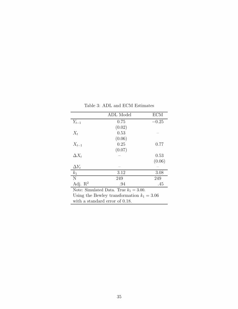
Table 3: ADL and ECM Estimates

ADL Model ECM

Yt−1 0.75 −0.25(0.02)

Xt 0.53 –(0.06)

Xt−1 0.25 0.77(0.07)

∆Xt – 0.53(0.06)

∆Yt – –k1 3.12 3.08N 249 249Adj. R2 .94 .45Note: Simulated Data. True k1 = 3.00.

Using the Bewley transformation k1 = 3.06with a standard error of 0.18.

35

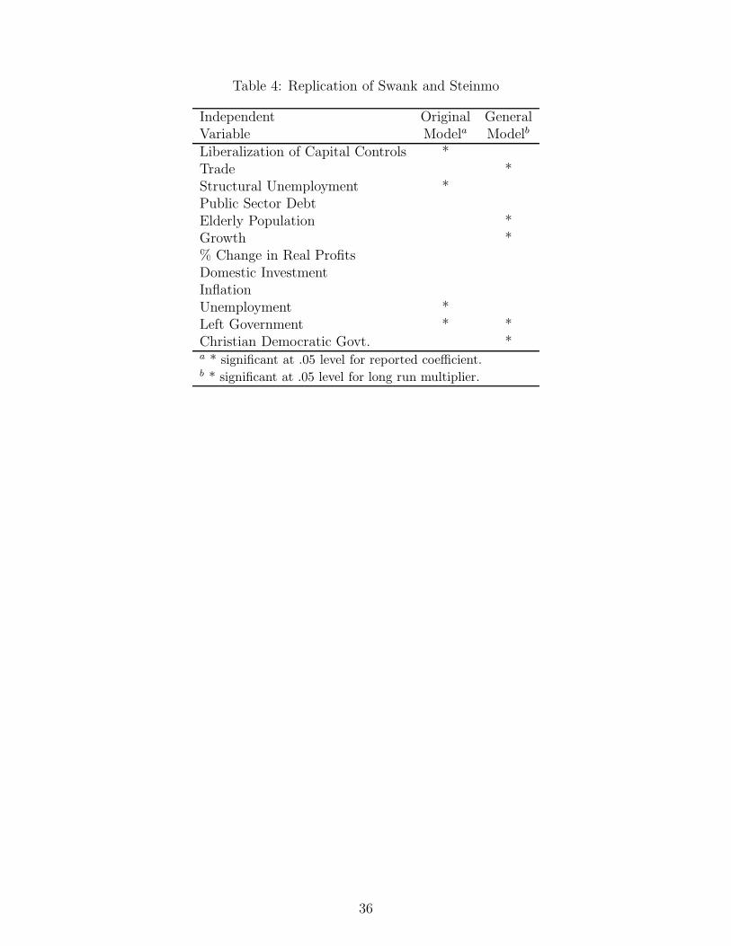
Table 4: Replication of Swank and Steinmo

Independent Original GeneralVariable Modela Modelb

Liberalization of Capital Controls *Trade *Structural Unemployment *Public Sector DebtElderly Population *Growth *% Change in Real ProfitsDomestic InvestmentInflationUnemployment *Left Government * *Christian Democratic Govt. *a * significant at .05 level for reported coefficient.b * significant at .05 level for long run multiplier.

36

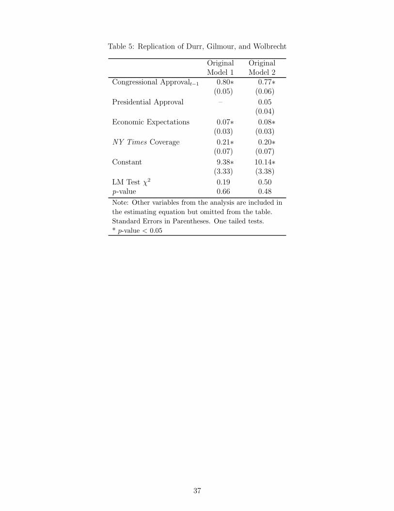
Table 5: Replication of Durr, Gilmour, and Wolbrecht

Original OriginalModel 1 Model 2

Congressional Approvalt−1 0.80∗ 0.77∗(0.05) (0.06)

Presidential Approval – 0.05(0.04)

Economic Expectations 0.07∗ 0.08∗(0.03) (0.03)

NY Times Coverage 0.21∗ 0.20∗(0.07) (0.07)

Constant 9.38∗ 10.14∗(3.33) (3.38)

LM Test χ2 0.19 0.50p-value 0.66 0.48

Note: Other variables from the analysis are included in

the estimating equation but omitted from the table.

Standard Errors in Parentheses. One tailed tests.

* p-value < 0.05

37

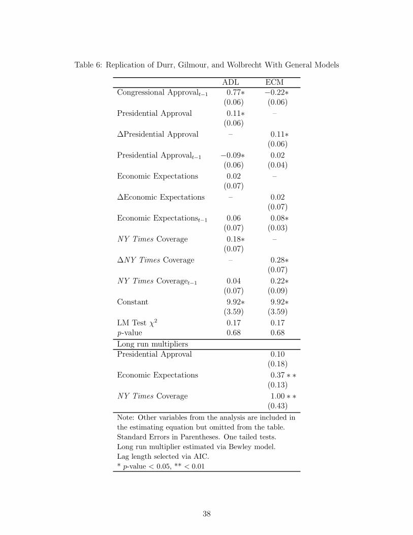
Table 6: Replication of Durr, Gilmour, and Wolbrecht With General Models

ADL ECMCongressional Approvalt−1 0.77∗ −0.22∗

(0.06) (0.06)

Presidential Approval 0.11∗ –(0.06)

∆Presidential Approval – 0.11∗(0.06)

Presidential Approvalt−1 −0.09∗ 0.02(0.06) (0.04)

Economic Expectations 0.02 –(0.07)

∆Economic Expectations – 0.02(0.07)

Economic Expectationst−1 0.06 0.08∗(0.07) (0.03)

NY Times Coverage 0.18∗ –(0.07)

∆NY Times Coverage – 0.28∗(0.07)

NY Times Coveraget−1 0.04 0.22∗(0.07) (0.09)

Constant 9.92∗ 9.92∗(3.59) (3.59)

LM Test χ2 0.17 0.17p-value 0.68 0.68

Long run multipliersPresidential Approval 0.10

(0.18)

Economic Expectations 0.37 ∗ ∗(0.13)

NY Times Coverage 1.00 ∗ ∗(0.43)

Note: Other variables from the analysis are included in

the estimating equation but omitted from the table.

Standard Errors in Parentheses. One tailed tests.

Long run multiplier estimated via Bewley model.

Lag length selected via AIC.

* p-value < 0.05, ** < 0.01

38

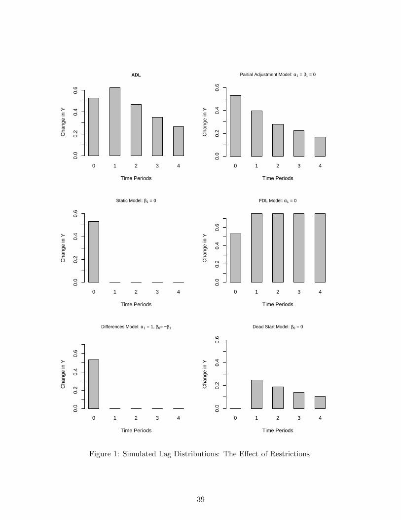
0 1 2 3 4

ADL

Time Periods

Cha

nge

in Y

0.0

0.2

0.4

0.6

0 1 2 3 4

Partial Adjustment Model: α1 = β1 = 0

Time Periods

Cha

nge

in Y

0.0

0.2

0.4

0.6

0 1 2 3 4

Static Model: β1 = 0

Time Periods

Cha

nge

in Y

0.0

0.2

0.4

0.6

0 1 2 3 4

FDL Model: α1 = 0

Time Periods

Cha

nge

in Y

0.0

0.2

0.4

0.6

0 1 2 3 4

Differences Model: α1 = 1, β0= −β1

Time Periods

Cha

nge

in Y

0.0

0.2

0.4

0.6

0 1 2 3 4

Dead Start Model: β0 = 0

Time Periods

Cha

nge

in Y

0.0

0.2

0.4

0.6

Figure 1: Simulated Lag Distributions: The Effect of Restrictions

39

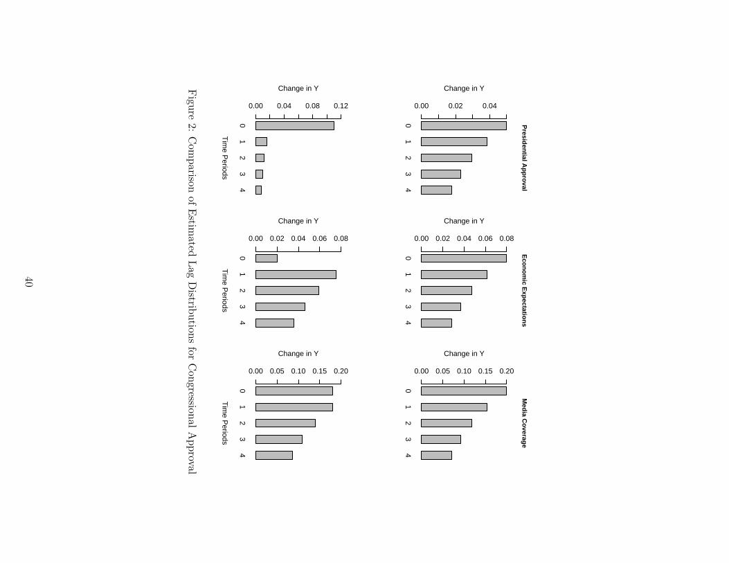
01

23

4

Presid

ential A

pp

roval

Change in Y

0.00 0.02 0.04

01

23

4

Eco

no

mic E

xpectatio

ns

Change in Y

0.00 0.02 0.04 0.06 0.08

01

23

4

Med

ia Co

verage

Change in Y

0.00 0.05 0.10 0.15 0.20

01

23

4

Tim

e Periods

Change in Y

0.00 0.04 0.08 0.12

01

23

4

Tim

e Periods

Change in Y

0.00 0.02 0.04 0.06 0.08

01

23

4

Tim

e Periods

Change in Y

0.00 0.05 0.10 0.15 0.20

Figu

re2:

Com

parison

ofE

stimated

Lag

Distrib

ution

sfor

Con

gressional

Approval

40