Taking in One Another’s Clothes? The Impact of Removal of ...
71
Conway/Fugazza -- 1 Draft; not for quotation Taking in One Another’s Clothes? The Impact of Removal of ATC Quotas on International Trade in Textiles and Apparel Patrick Conway Marco Fugazza Department of Economics Trade Analysis Branch University of North Carolina UNCTAD Chapel Hill, NC 27599-3305 Geneva, Switzerland [email protected] [email protected] Revision: July 2010 Abstract: Theory predicts that a system of bilateral quotas such as observed in the Agreement on Textiles and Clothing (ATC) will cause both trade diversion and trade deflection, with an end result of more trading partners and smaller values traded on average than in the absence of the quotas. Quota removal will reverse this process, leading to trade creation and the focusing of trade in larger values by a smaller group of exporters. We derive these predictions from a micro-founded model of bilateral trade, and we test these predictions in a panel database of trade among 126 world trading partners in cotton textiles and apparel for the period 1994-2006. We find evidence of both trade diversion and trade deflection in this period governed by quotas. The quota system was largely removed at the beginning of 2005. We use the model estimated for the quota-system years to predict bilateral trade in textiles and apparel in 2005 (out of sample). We do not find evidence of trade focus on average. This aggregate non-result is shown to be due to the averaging of the anticipated trade-creation effect among a small group of low-comparative-cost exporters and the opposite, trade-rediverting, effect among a larger group of countries displaced from sales in the US and EU by the removal of quotas. This research was begun while Conway was a visitor at the Trade Analysis Branch of UNCTAD in Geneva, and he thanks the staff for its hospitality and support during that time. Thanks to Michiko Hayashi for comments on an earlier version.
Transcript of Taking in One Another’s Clothes? The Impact of Removal of ...
Conway/Fugazza -- 1
Draft; not for quotation
Taking in One Another’s Clothes? The Impact of Removal of ATC Quotas on International Trade in Textiles and Apparel
Patrick Conway Marco Fugazza Department of Economics Trade Analysis Branch University of North Carolina UNCTAD Chapel Hill, NC 27599-3305 Geneva, Switzerland [email protected] [email protected] Revision: July 2010 Abstract: Theory predicts that a system of bilateral quotas such as observed in the Agreement on Textiles and Clothing (ATC) will cause both trade diversion and trade deflection, with an end result of more trading partners and smaller values traded on average than in the absence of the quotas. Quota removal will reverse this process, leading to trade creation and the focusing of trade in larger values by a smaller group of exporters. We derive these predictions from a micro-founded model of bilateral trade, and we test these predictions in a panel database of trade among 126 world trading partners in cotton textiles and apparel for the period 1994-2006. We find evidence of both trade diversion and trade deflection in this period governed by quotas. The quota system was largely removed at the beginning of 2005. We use the model estimated for the quota-system years to predict bilateral trade in textiles and apparel in 2005 (out of sample). We do not find evidence of trade focus on average. This aggregate non-result is shown to be due to the averaging of the anticipated trade-creation effect among a small group of low-comparative-cost exporters and the opposite, trade-rediverting, effect among a larger group of countries displaced from sales in the US and EU by the removal of quotas. This research was begun while Conway was a visitor at the Trade Analysis Branch of UNCTAD in Geneva, and he thanks the staff for its hospitality and support during that time. Thanks to Michiko Hayashi for comments on an earlier version.

Conway/Fugazza -- 2
On 1 January 2005 the United States (US), Canada and the European Union (EU) eliminated
a system of bilateral quotas on imports of textiles and apparel. These quota constraints had been in
use in some form since the early 1960s.1 The phased elimination of the quotas was codified in the
Agreement on Textiles and Clothing (ATC) of the World Trade Organization (WTO) during the
period 1995-2004. While these quotas were welfare-reducing for the residents of these areas, they
also had the effect of stimulating exports of textiles and apparel from a number of developing
economies that might otherwise not have participated in those import markets. This effect is “trade
diversion” (as Viner (1950) characterized it) for the importing countries and a growth stimulus for
the developing-country exporters. There is also the potential for “trade deflection” and “trade
destruction”, as Bown and Crowley (2007) predict: countries facing a binding quota from these
areas will then either deflect their products to third countries or reduce their imports from third
countries by substituting in domestic production.
Viner would have straightforward predictions for trade patterns and volumes in the quota-
levying countries once these quotas were removed: exporter status would be determined by
comparative advantage, and larger-volume imports on average would be observed from the same or
fewer exporters. To the extent that quota liberalization increased world demand for the products,
“world” prices would rise while the liberalized prices in the quota-levying countries would fall. This
rise in “world price” would cause supply and demand adjustments throughout the world trading
economies.
We find something quite different when we examine the international trade in cotton
clothing and textiles with the elimination of quotas: there is an expansion on average in the number
of trading partners in both textiles and apparel, and a reduction in the average value of trade
conducted bilaterally. This is the conundrum referenced in the title: why are countries taking in less
textiles and clothing from even more trading partners with the removal of the quota system?
The impact of the removal of ATC quotas on prices and volumes imported into the US and
EU markets has been studied elsewhere. We are interested in this paper in the third-country effects
of quota liberalization. Many developing and transition economies around the world created an
export-led growth strategy around textiles and apparel during the years leading up to 2005. By study
of this episode we can evaluate the effectiveness of that strategy.
To decompose the empirical third-party effects of quota liberalization we create a micro-
founded model of trade flows based upon the heterogeneous-firm approach of Helpman, Melitz and
Rubenstein (2008, hereafter HMR). We estimate this model in the quota period 1994-2004 for a
1 The Long-Term Arrangement in Cotton Textiles (LTA) in the US was the first incidence of these quotas; they were regularized and extended to other fibers in the Multi-Fiber Arrangement (MFA) from 1974 to 1995,

Conway/Fugazza -- 3
sample of 126 developed and developing countries, and then use the removal of quotas in 2005 as an
experiment to identify the refocusing of trade predicted by theory relative to the pattern of the quota-
period model. While we do not measure welfare effects explicitly, we are able to track the country-
specific evolution in export expansion or contraction.
Our estimation results identify reasonable parameters for the structural model as well as the
Vinerian logic of trade diversion in the data. We also identify “trade rediversion” among those
countries that benefited from access to the US and EU countries during the quota period: their
response to quota removal has been to redirect their exports to larger numbers of other countries in
search of markets to replace those of the US and EU. The “comparative advantage” exporters
(including the major Asian exporters) in these two industries did not expand the number of trading
partners and did increase the average volume of trade per exporter, just as theory predicts. By
contrast, the countries that became exporters of textiles and apparel because of the quota system did
not shut down. Instead, they sold smaller volumes of their goods to more peripheral markets.
Our attention to the general-equilibrium and third-country effects of removal of quotas
distinguishes our work from two recent papers on the removal of the ATC quotas. Harrigan and
Barrows (2006) examined the difference in price and quality for US imports in a difference-in-
difference framework for the top 20 exporters to the US: there is the time difference, from 2004 to
2005, and the categorical difference in quota-constrained vs. unconstrained imports.2 The authors
first measure the average adjustment in price and quality for each country in the sample; they find a
substantial downward average adjustment in price for quota-constrained imports and a much smaller
downward adjustment in quality. There are no such downward adjustments for unconstrained
imports. The authors then test across countries to determine whether the adjustments in price and
quality from 2004 to 2005 are on average significantly different for constrained than for
unconstrained categories. The downward price adjustments are statistically significant for all
exporters at the 95 percent level of confidence, for China alone and for the non-China exporters.
The downward quality adjustments are significant for China alone and for all exporters at the 90
percent level of confidence. This work is done at a quite detailed level of disaggregation, and
signals the expected impact of quota removal on both price and quality. It treats the observation of a
binding quota as an exogenous event, however – and this can introduce bias.
Brambilla, Khandelwal and Schott (2007) focus their attention on exporters of textiles and
apparel to the US. They work as well with 10-digit HS data on imports from these countries into the
2 The unit for imports is the HS 10 classification. Each classification is designated as either “constrained” or “unconstrained” depending upon whether that classification is part of a quota category binding for that exporter in that year.

Conway/Fugazza -- 4
US, and they also categorize the imports as being quota-constrained vs. unconstrained using the US
quota classifications. They analyze carefully the impact of the quota, and then contrast that with
behavior after quota removal: they are careful to distinguish the four stages of sequential quota
elimination under the ATC, and to connect the changes in quantity and price with the appropriate
stage of quota removal. They find both an increase in quantity and a reduction in price for Chinese
goods that is significantly different from that observed in other quota-constrained exporters. They
do not calculate quality as in Harrigan and Barrows (2006), and thus cannot draw conclusions on the
impacts of price vs. quality. They also treat the quota-constrained period as an exogenous event.
Our approach to the removal of quotas represents both an extension and an aggregation of
the results of these two papers. We extend these conceptually by considering the general-
equilibrium effects of bilateral trade among all countries, not just those that impose quotas. We
model the production/trade relationship between textiles and clothing. We also extend the analysis
technically by recognizing that a binding quota will be an endogenous event in this model. On the
other hand, we use more aggregated data than the 10-digit HS level used by these two papers. We
create an indicator of quota limits and binding quotas based upon aggregating up from the individual
quota categories defined by the US and the EU. Details on this procedure are provided in the text
and data appendices.
I. Taking in each other’s clothing (and textiles).
There is great variation in the participation of countries as exporters in the world markets for
cotton textiles and apparel, as is evident in Figures 1 and 2. For these figures, the 126 countries in
the sample are sorted for each year in ascending order by number of importing trading partners. 3
The vertical axis indicates the share of the 126 countries to which each country exports. The blue
dashed line indicates the distribution in 2004. There are six countries not exporting at all, and 55
countries that export to no more than 10 percent of the trading countries. At the upper extreme, the
best-connected exporter (China) sells into over 90 percent of the markets considered.
We could operationalize the Vinerian prediction in response to quota elimination by positing
that post-quota this curve will shift down: the comparative-advantage exporters will focus upon the
countries in which quotas limited them, thus discarding periphery markets. The non-comparative-
advantage exporters at the lower end of the spectrum would see their access to the previously quota-
3 We examine in this section aggregate cotton textiles (SITC 652) and apparel (SITC 841 & 842) trade for 126 countries during this period. This is also the sample used in the estimation of part III. COMTRADE does report data on bilateral trade for 169 countries; those excluded are small and not major trading partners. (Italy is the exporter with the most trading partners in the larger sample, reaching 83 and 86 percent of importer countries in textiles and apparel, respectively.)
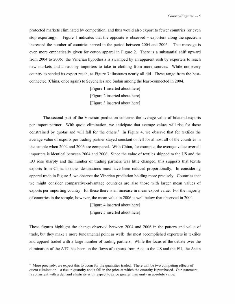
Conway/Fugazza -- 5
protected markets eliminated by competition, and thus would also export to fewer countries (or even
stop exporting). Figure 1 indicates that the opposite is observed – exporters along the spectrum
increased the number of countries served in the period between 2004 and 2006. That message is
even more emphatically given for cotton apparel in Figure 2. There is a substantial shift upward
from 2004 to 2006: the Vinerian hypothesis is swamped by an apparent rush by exporters to reach
new markets and a rush by importers to take in clothing from more sources. While not every
country expanded its export reach, as Figure 3 illustrates nearly all did. These range from the best-
connected (China, once again) to Seychelles and Sudan among the least-connected in 2004.
[Figure 1 inserted about here]
[Figure 2 inserted about here]
[Figure 3 inserted about here]
The second part of the Vinerian prediction concerns the average value of bilateral exports
per import partner. With quota elimination, we anticipate that average values will rise for those
constrained by quotas and will fall for the others.4 In Figure 4, we observe that for textiles the
average value of exports per trading partner stayed constant or fell for almost all of the countries in
the sample when 2004 and 2006 are compared. With China, for example, the average value over all
importers is identical between 2004 and 2006. Since the value of textiles shipped to the US and the
EU rose sharply and the number of trading partners was little changed, this suggests that textile
exports from China to other destinations must have been reduced proportionally. In considering
apparel trade in Figure 5, we observe the Vinerian prediction holding more precisely. Countries that
we might consider comparative-advantage countries are also those with larger mean values of
exports per importing country: for these there is an increase in mean export value. For the majority
of countries in the sample, however, the mean value in 2006 is well below that observed in 2004.
[Figure 4 inserted about here]
[Figure 5 inserted about here]
These figures highlight the change observed between 2004 and 2006 in the pattern and value of
trade, but they make a more fundamental point as well: the most accomplished exporters in textiles
and apparel traded with a large number of trading partners. While the focus of the debate over the
elimination of the ATC has been on the flows of exports from Asia to the US and the EU, the Asian
4 More precisely, we expect this to occur for the quantities traded. There will be two competing effects of quota elimination – a rise in quantity and a fall in the price at which the quantity is purchased. Our statement is consistent with a demand elasticity with respect to price greater than unity in absolute value.
Conway/Fugazza -- 6
exporters are involved in sales to many more countries than these – in fact, to a majority of the
countries in the sample. Tables 1 and 2 indicate the number of countries receiving exports from
seven major exporters of textiles and apparel, respectively. The six Asian countries presented in the
table have customers in a great majority of the countries of the world – as does the US. Most
countries do not have this great diversification of exports – in fact, in 2004, 69 percent of apparel
exporters and 85 percent of textiles exporters sold to fewer than half the countries in the sample.
The export business is also not driven solely by low labor cost: the lists of top-20 exporters in terms
of number of markets served include a large number of developed countries.5
Table 3 provides a final illustration of the conundrum we observe in the world market
response to quota elimination. If our extension of Viner’s logic to the world economy were correct,
we’d anticipate a refocusing of trade in the aftermath of liberalization: fewer lower-cost exporters
shipping more on average to each partner. Table 3 contradicts this logic. The proportion of bilateral
trading partners in the sample for which positive (i.e., value greater than zero) exports are observed
is rising throughout the period, but it continues to rise in 2005 and 2006. To understand this
conundrum, we must examine the pattern and value of trade in a structural model that allows us to
separate the Vinerian aspects of quota removal from other driving factors.
II. Modeling the bilateral import-export decision.
To identify the impact of quotas on the pattern and volume of bilateral trade, it is necessary
to control for the other factors determining trade in these goods. In this section we provide a
structural model of the decision to import from one country to another adapted from HMR to the
features of world trade in textiles and apparel.
A. Consumer demand. In country j and in time t, each individual b consumes a quantity
ξbjt(ν) of each variety ν of textiles (or apparel) from a continuum of varieties along the interval [0 β],
with β the share of individual income spent on these varieties. He derives utility in a Dixit and
Stiglitz (1977) aggregator as below:
Ubjt = {∫ ξbjt(ν)α dν}(1/α) 0 < α < 1 (1)
and optimizes subject to variety price pjt(ν) and budget constraint βYbjt = ∫ pjt(ν) ξbjt(ν) dν.
If Yjt = Σb Ybjt is the real income of country j in time t, then the country-j expenditure for variety ν is
5 In apparel, six of the top 10 exporters in terms of numbers of trading partners are developed countries (Italy, Germany, France, Spain, UK and US). In textiles, seven of the top 10 exporters in terms of numbers of trading partners (those above plus Belgium) are developed countries.

Conway/Fugazza -- 7
pjt(ν) xjt(ν) = pjt(ν) Σb ξbjt(ν) = [pjt(ν)/Pjt]1-ε βYjt
(2)
Pjt = { ∫ pjt(ν)1-ε dν} 1/(1-ε) (3)
Where pjt(ν) is the price of variety ν in country j at time t.6 Pjt is the sector’s ideal price index, and
every product ν has a constant price elasticity ε = (1/(1-α)) defined to be positive.7 These goods
could either be locally produced or produced in foreign countries.
B. Quality divergences from pjt(ν). The country-j market is an imperfectly competitive
one, but pijt(υ) can diverge from the country-j average pjt(υ) if there are differences in country-
specific quality. With quality denoted by θi for each exporter i (and average quality given value of
1), the equilibrium prices in importer j in period t will have the relation defined in (4).
pijt(υ)/ θi = pjt(υ) for each variety υ without quota (4)
C. Producer characteristics. Suppliers create each product through use of labor. The
total cost of production for an individual supplier f is given in labor units as
Cfit(ν) = citaf(ν)xf(ν) + NftcitFfit(ν) (5)
The first element of the summation is the variable cost, with xf(ν) as a measure of total production.8
The second element is the fixed cost of producing for export; it will be the fixed costs for exporting
to one market Ffit(ν) times the number of export markets (Nft).9 For each variety ν there is a
distribution of suppliers in each country. Supplier-level heterogeneity is decomposed into two parts.
First, there is a global distribution of technology. We use labor input per unit of output (or the
6 This derivation is appropriate for differentiated products with the same quality. If the differentiated products differ as well along a quality dimension, Hallak (2006) demonstrates that a similar derivation will hold with ξbjt and pjt(ν) defined in quality-adjusted units. For example, if quality of goods from supplier i is defined θi and the price of product ν from supplier i to country j is pijt(ν) , then pjt(ν) xjt(ν) = (pijt(ν)/θi)
1-ε Yjt/Pjt1-ε, where Pjt =
{ ∫ (pijt(ν)/θi) 1-ε dν} 1/(1-ε) . We return to this point in the next section.
7 As Novy (2010) points out, this CES assumption is a restrictive specification. Novy uses a translog gravity function and data from 28 OECD countries between 1991 and 2000 to point out that a more general form will lead to systematic variability in the elasticity of trade with respect to transport costs. We intend to investigate the importance of this for our analysis in future research. 8 Given the producer’s technology, we assume that it is either producing at full capacity or not producing at all. 9 This fixed cost is exemplified by the distribution network that an exporter must establish prior to servicing a new market.
Conway/Fugazza -- 8
inverse of productivity) as the index, denoted by “a”. (Low values of “a” represent low-cost, or
high-productivity, firms, and high values represent the converse.) All suppliers worldwide have
technology defined by a supplier-specific draw af from the time-invariant distribution g(a) bounded
in the range [aL aH]. Second, there is a country-level difference in production cost cit that scales up or
down the productivity of all suppliers in that country. Consider a continuum of suppliers in country i
at time t. The per-unit variable cost of each country-i firm in time t is defined citaf(ν). Each supplier
f in country i will have unit cost vfit(ν) = cit af(ν) in selling in the domestic market and vfijt(ν) = cit
af(ν) + Ffit(ν)/xf(ν) in exporting to a foreign country.10
If country j imposes binding quotas qkjt(ν) < xkjt(ν) on the quantity imported from country k
in period t, then the quantity imported from country k will be less than the optimal quantity defined
by (2) for this variety. This will lead to the protection of domestic industry, the deadweight losses
associated with quotas, and a wedge between the price received by the producer and the price paid
by the purchaser. τijt is one plus the tax-equivalent percent of the wedge created by a binding quota
by country j on country-i goods. 11 Without loss of generality, we define a share χij that is
transmitted through to an increase in pjt(ν), the average price of the import variety subject to the
quota in country j.12 The remainder share is transmitted to country-j exporters through lower
effective price received for exports.
Not all producers will export to all countries. Define Πijt(ν) as supplier profits due to
exporting from country i to country j in period t. The zero-profit condition in (6) defines the lowest-
productivity firm aoijt(ν) able to export variety ν to country j. A definition of this productivity level is
reported in (7).
Πijt(ν) = [pijt(ν)/[τijt (1+sijt)(1+tijt)] – citao
ijt(ν)] xf (ν) – cit Ffit(ν) = 0 (6)
{(θi/cit)pjt(υ)/[τijt (1+sijt)(1+tijt)]} - Ffit(ν)/ xf (ν) = aoijt(ν) (7)
sijt is the percent shipping cost from country i to country j and tijt is the ad valorem tariff (or tariff-
equivalent of a non-tariff barrier) imposed by country j on the products of country i. As shipping
10 The total fixed cost Ffit = Σj Fijt, where j is summed over the set of countries to which the supplier exports. 11 It is simplest to think of this as the ratio of the landed price of the good divided by the exporter effective price augmented by transportation costs. The difference is the price of a tradable permit purchased by the producer to export one unit under the quota. The cost of this permit will be considered among the operating costs of the firm, and will reduce its profits. (If the firm is itself the owner of the quota, it will nevertheless be in its interests to consider the permit as an asset to be used or rented – if possible – at a market price.) An alternative model will include quota rents accruing to the exporting country. These rents will raise the rent-inclusive price of the export, and will have different implications for trade patterns. 12 I.e., dpjt = (pjt χij/τijt) dτijt and the effective exporter price is pjt /τijt with d(pjt /τijt )/dτijt = -(1-χij) pjt dτijt

Conway/Fugazza -- 9
costs, country-specific production costs, fixed costs or tariffs rise, the critical aoijt(ν) will fall (i.e., the
necessary productivity level to be an exporter to j will rise). As pjt(ν), the average import price in
country j, rises or country-specific quality rises, aoijt(ν) will rise. For suppliers in country i with high-
productivity draws af < aoijt there will be non-negative profits in exporting to country j; for firms with
af > aoijt there will be no exporting to country j. Since the cut-off differs by trading partner, those
firms in country i unable to export to country j may be able to export to country k so long as their
observed “a” falls in the range [aoijt a
oikt].
Note the important end-point restrictions. The calculation in (6) puts no limits on aoijt, but
we know that “a” is drawn from the range [aL aH]. If aoijt < aL, this indicates that none of the country-
i suppliers can be profitable in selling to country j. If aoijt > aH, then all country-i suppliers will be
profitable in selling in the country-j market.
D. Equilibrium in country j for variety ν. Demand for variety ν in country j is given by
xjt(ν) in equation (2). Supply of variety ν to country j is determined by the individual firms’ zero-
profit conditions in equation (6). As the price pjt(ν) at which the variety can be sold rises, aoijt(ν)
rises. This increases (or at worst leaves constant) the number of suppliers in country i willing to
export to country j.
The supply from country i to country j (Xijt) and the total supply to country j (Xjt) of variety
ν can be defined:
Xijt(ν) = aL ∫ aoijt(ν) xf(ν) g(a) da (8)
Xjt(ν) = Σi Xijt(ν) (9)
Note that both Xijt(ν) and Xjt(ν) are non-decreasing in the price pjt(ν) through the “cut-off”
productivity values aoijt(ν).
Equilibrium in country j in the market for variety υ is defined by the equality of supply and
demand:
Xjt(ν) = xjt(ν) (10)
The equilibrium pjt(ν) and aoijt(ν) are jointly determined through the zero-profit condition for each
supplier country. This equilibrium is not determined in isolation: firms potentially supplying variety ν
will also consider exporting to other countries, and will be competing for scarce resources with
suppliers of other varieties – and other goods. The set {pjt(ν), aoijt(ν)} equilibrate to leave country i at
Conway/Fugazza -- 10
full employment.13 As different varieties are uniquely associated with different countries, we suppress
the index for variety in the sections that follow.
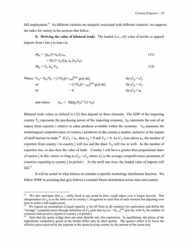
E. Deriving the value of bilateral trade. The landed (i.e., cif) value of textile or apparel
imports from i into j in time t is
Mijt = [pijt/(1+tijt)] xijt (11)
= [θi/(1+tijt)] pjt xjt{xijt/xjt}
Mijt = Yjt Δijt Vijt (12)
Where Vijt = Xijt/Xjt = (1/Njt)[1+aojt∫aoijt
g(a) da] for aoijt > ao
jt
or = (1/Njt)[1- aoijt∫aojt g(a) da] for ao
ijt < aojt
or = 0 for aoijt < aL
and where Δijt = θiβ(pjt/Pjt)1-ε/(1+tijt)
Bilateral trade values as defined in (12) thus depend on three elements. The GDP of the importing
country Yjt represents the purchasing power of the importing economy. Δijt represents the cost of an
import from exporter i relative to other products available within the economy. Vijt measures the
technological competitiveness of country-i producers in the country-j market, inclusive of the impact
of tariff barriers to trade.14 If aoijt < aL, then xijt = 0 and Vijt = 0. As ao
ijt rises above aL, the number of
exporters from country i to country j will rise and the share Vijt will rise as well. As the number of
exporters rise, so also does the value of trade. Country i will have a greater than proportional share
of market j in this variety so long as aoijt > ao
jt, where aojt is the average competitiveness parameter of
countries exporting to country j in period t. As the tariff rate rises, the landed value of imports will
fall.15
It will be useful in what follows to consider a specific technology distribution function. We
follow HMR in assuming that g(a) follows a constant Pareto distribution across time and country.
13 We also anticipate that cit , while fixed at any point in time, could adjust over a longer horizon. One interpretation of cit is as the labor cost in country i, exogenous to each firm at each moment but adjusting over time to achieve full employment. 14 We impose an assumption of equal capacity xf for all firms in all countries for explication, and define the “average” competitiveness through definition of ao
jt such that (xjt/xf) = Njt aL∫aojt g(a) da, with Njt the number of
countries with positive exports to country j in period t. 15 Note that the quota wedge does not enter directly into this expression. In equilibrium, the prices of the imperfectly competitive goods at the border differ only by their quality. The quota’s effect is to lower the effective price received by the exporter in the quota-levying country by the amount of the quota rent.
Conway/Fugazza -- 11
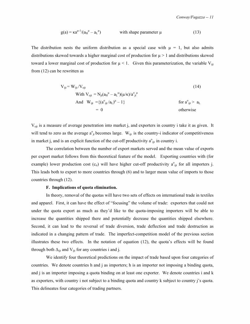
g(a) = κaµ-1/(aHµ – aL
µ) with shape parameter µ (13)
The distribution nests the uniform distribution as a special case with µ = 1, but also admits
distributions skewed towards a higher marginal cost of production for µ > 1 and distributions skewed
toward a lower marginal cost of production for µ < 1. Given this parameterization, the variable Vijt
from (12) can be rewritten as
Vijt = Wijt /Vojt (14)
With Vojt = Njt(aHµ – aL
µ)(µ/κ)/aojt
µ
And Wijt ={(aoijt /aL)µ – 1} for ao
ijt > aL
= 0 otherwise
Vojt is a measure of average penetration into market j, and exporters in country i take it as given. It
will tend to zero as the average aojt becomes large. Wijt is the country-i indicator of competitiveness
in market j, and is an explicit function of the cut-off productivity aoijt in country i.
The correlation between the number of export markets served and the mean value of exports
per export market follows from this theoretical feature of the model. Exporting countries with (for
example) lower production cost (cit) will have higher cut-off productivity aoijt for all importers j.
This leads both to export to more countries through (6) and to larger mean value of imports to those
countries through (12).
F. Implications of quota elimination.
In theory, removal of the quotas will have two sets of effects on international trade in textiles
and apparel. First, it can have the effect of “focusing” the volume of trade: exporters that could not
under the quota export as much as they’d like to the quota-imposing importers will be able to
increase the quantities shipped there and potentially decrease the quantities shipped elsewhere.
Second, it can lead to the reversal of trade diversion, trade deflection and trade destruction as
indicated in a changing pattern of trade. The imperfect-competition model of the previous section
illustrates these two effects. In the notation of equation (12), the quota’s effects will be found
through both Δijt and Vijt for any countries i and j.
We identify four theoretical predictions on the impact of trade based upon four categories of
countries. We denote countries h and j as importers; h is an importer not imposing a binding quota,
and j is an importer imposing a quota binding on at least one exporter. We denote countries i and k
as exporters, with country i not subject to a binding quota and country k subject to country j’s quota.
This delineates four categories of trading partners.
Conway/Fugazza -- 12
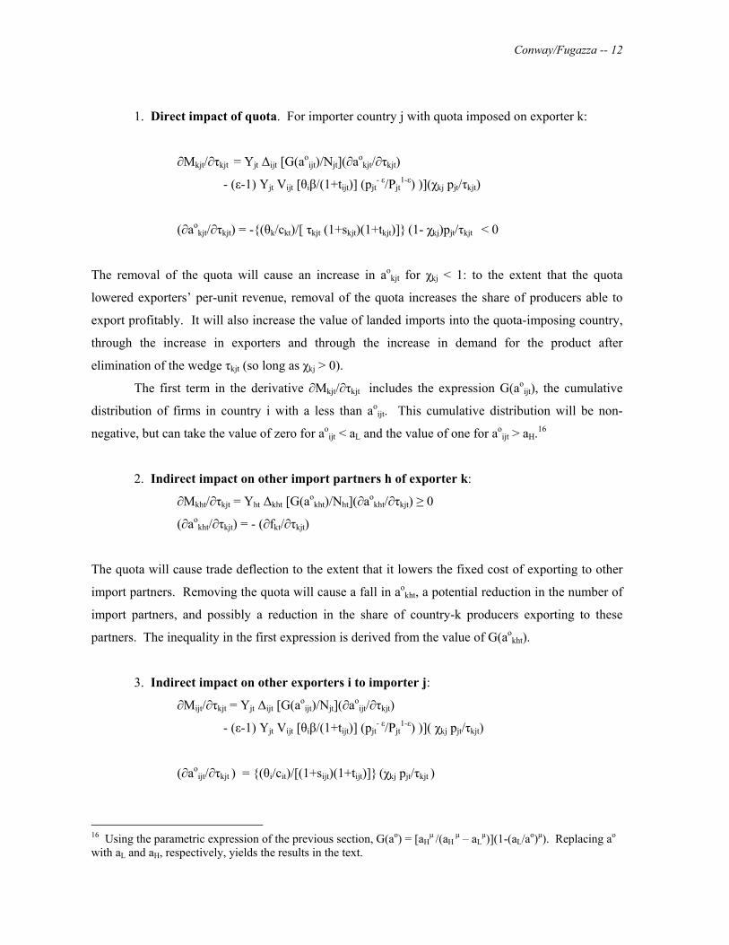
1. Direct impact of quota. For importer country j with quota imposed on exporter k:
∂Mkjt/∂τkjt = Yjt Δijt [G(aoijt)/Njt](∂ao
kjt/∂τkjt)
- (ε-1) Yjt Vijt [θiβ/(1+tijt)] (pjt- ε/Pjt
1-ε) )](χkj pjt/τkjt)
(∂aokjt/∂τkjt) = -{(θk/ckt)/[ τkjt (1+skjt)(1+tkjt)]} (1- χkj)pjt/τkjt < 0
The removal of the quota will cause an increase in aokjt for χkj < 1: to the extent that the quota
lowered exporters’ per-unit revenue, removal of the quota increases the share of producers able to
export profitably. It will also increase the value of landed imports into the quota-imposing country,
through the increase in exporters and through the increase in demand for the product after
elimination of the wedge τkjt (so long as χkj > 0).
The first term in the derivative ∂Mkjt/∂τkjt includes the expression G(aoijt), the cumulative
distribution of firms in country i with a less than aoijt. This cumulative distribution will be non-
negative, but can take the value of zero for aoijt < aL and the value of one for ao
ijt > aH.16
2. Indirect impact on other import partners h of exporter k:
∂Mkht/∂τkjt = Yht Δkht [G(aokht)/Nht](∂ao
kht/∂τkjt) ≥ 0
(∂aokht/∂τkjt) = - (∂fkt/∂τkjt)
The quota will cause trade deflection to the extent that it lowers the fixed cost of exporting to other
import partners. Removing the quota will cause a fall in aokht, a potential reduction in the number of
import partners, and possibly a reduction in the share of country-k producers exporting to these
partners. The inequality in the first expression is derived from the value of G(aokht).
3. Indirect impact on other exporters i to importer j:
∂Mijt/∂τkjt = Yjt Δijt [G(aoijt)/Njt](∂ao
ijt/∂τkjt)
- (ε-1) Yjt Vijt [θiβ/(1+tijt)] (pjt- ε/Pjt
1-ε) )]( χkj pjt/τkjt)
(∂aoijt/∂τkjt ) = {(θi/cit)/[(1+sijt)(1+tijt)]} (χkj pjt/τkjt )
16 Using the parametric expression of the previous section, G(ao) = [aH
μ /(aH μ – aL
μ)](1-(aL/ao)μ). Replacing ao with aL and aH, respectively, yields the results in the text.

Conway/Fugazza -- 13
The price pjt rose in the quota-imposing country (so long as χkj > 0). Removing the quota will cause
pjt to fall. This will have offsetting effects on exports from country i. First, there is the reversal of
trade diversion: it reduces the measure of producers aoijt in exporter i able to sell into importer j (and
perhaps eliminates i as an exporter). Second, the country-j demand for these products will rise due
to the reduced price of these exports, and this will be reflected ceteris paribus in increased exports
from country i.
4. Indirect impact on other import partners h and other exporters i:
∂Miht/∂τkjt = 0
(∂aoiht/∂τkjt ) = 0
These are the Vinerian substitution effects that we anticipate from quota removal. Given the size
and market share of the quota-levying countries, we should add to these the potential general-
equilibrium effects on pjt for each importer j.17 Removal of the bilateral quotas will increase demand
for textiles and apparel and thus increase the observed pjt for non-quota-levying countries.18
5. General-equilibrium effects for other import partners h and other exporters i:
∂aoiht/∂pht > 0
∂Miht/∂pht < 0 for ε > 1
The last comparative static suggests that ignoring general-equilibrium effects on final-good
prices in importing countries or production cost in exporting economies (e.g., wages) will limit the
explanatory power of the model. The conundrum of the introductory section suggested that
increased export reach was a characteristic of many countries, not just the subset with comparative
advantage.
III. Estimation.
The model of imperfect competition presented in the previous section provides a
parsimonious summary of possible determinants of trade pattern and value. Our hypothesis is that
17 Staritz (2010), using COMTRADE data, reports that the US and fifteen-member EU together represented over 67 percent of total world imports of apparel in both 1995 and 2005. For textiles, the percent is xxx; not as large, but nevertheless a substantial portion of the market. 18 Viner (1950) did not address this terms-of-trade argument, but Meade (1956) and Lipsey (1957) did. Conway, Appleyard and Field (1989) provide an exposition of the point in a continuum-of-goods model.

Conway/Fugazza -- 14
elimination of the quota system in the US and EU has had significant effects on the pattern and value
of international trade in textiles and apparel. We specifically anticipate that the elimination of
quotas will eliminate the patterns of trade diversion, trade deflection and trade destruction that
theory predicted as outcomes in the presence of binding quotas. Our estimation strategy is
complicated by the fact that we begin from a quota-ridden environment: the “experiment” examined
here is the movement from the distorted market to a non-distorted market. It is further complicated
by the fact that quotas were removed in four steps, in 1995, 1998, 2002 and 2005. The final two
steps were the most important in terms of quantitative impact, but there could also be an
“announcement effect” on trade patterns from the introduction of the quota-elimination plan under
the ATC in 1995.
Equations (7) and (12) define the landed value of bilateral imports and the decision on
whether to export on a bilateral basis as functions of the structural parameters and variables of this
model. These serve as the basis of our estimation technique. Our modeling strategy is quite similar
to that of HMR, and thus it is instructive to consider their identification strategy. In HMR, there are
stochastic components to fixed and iceberg trade costs, and the first appears only in the export-
decision equation (6). The authors introduce a regulation-cost variable to instrument for the
unobserved fixed-cost effect.19 The authors check the robustness of this strategy by introducing a
second instrument (religion) for fixed cost and verify that their estimation results are insensitive to
choice of instrument.
We follow a similar approach, but use a bifurcation of the data to ensure proper
identification. The ratio (aoijt/aL) is the critical determinant of the pattern of bilateral trade in
equilibrium from country i to country j in period t. Combining (12) with (6) yields an expression for
the unobserved aoijt/aL.20
ln(aoijt/aL) = ln(pjt) - ln(aL) – [ln(cit/θi)] - sijt - τijt - tijt
– fijt (15)
The transport cost ratio (sijt) is not observed annually, but in (16) is proxied by an iceberg model with
shipping costs proportional to distance (Dij), with an indicator variable for adjacent countries (DBij)
to capture the potentially lower shipping costs due to propinquity, and with year-specific variation
picked up by year-specific dummy variables Ht. The exporter cost/quality ratio ln(cit/θi) is treated in
(17) as a stochastic variable with exporter-specific value ĉi and random component ζijt. The binding
19 Identification of the coefficients in the import volume equation is also assured by the non-linear nature of the estimation equation, a product of the specific Pareto distribution assumed for unobserved productivity. 20 In this expression, we also use the approximations sijt = ln(1+sijt) and tijt= ln(1+tijt). These are used for exposition, but not in estimation. We define fijt=ln(Fijt/xfaL).
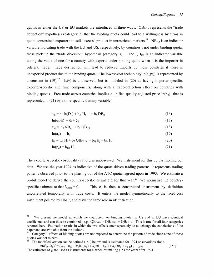
Conway/Fugazza -- 15
quotas in either the US or EU markets are introduced in three ways. QBiNUt represents the “trade
deflection” hypothesis (category 2) that the binding quota could lead to a willingness by firms in
quota-constrained exporter i to sell “excess” product in unrestricted markets.21 NBiUt is an indicator
variable indicating trade with the EU and US, respectively, by countries i not under binding quota:
these pick up the “trade diversion” hypothesis (category 3). The QBUjt is an indicator variable
taking the value of one for a country with exports under binding quota when it is the importer in
bilateral trade: trade destruction will lead to reduced imports by those countries if there is
unexported product due to the binding quota. The lowest-cost technology ln(aL(ν)) is represented by
a constant in (19).22 fijt(ν) is unobserved, but is modeled in (20) as having importer-specific,
exporter-specific and time components, along with a trade-deflection effect on countries with
binding quotas. Free trade across countries implies a unified quality-adjusted price ln(pjt) that is
represented in (21) by a time-specific dummy variable.
sijt = b1 ln(Dij) + b2t Ht + b3 DBij (16)
ln(cit/θi) = ĉi + ζijt (17)
τijt = b4 NBiUt + b5 QBUjt (18)
ln(aL) = - bo (19)
fijt = b6i Hi + b7 QBiNUit + b8j Hj + b9t Ht (20)
ln(pjt) = b10t Ht (21)
The exporter-specific cost/quality ratio ĉi is unobserved. We instrument for this by partitioning our
data. We use the year 1994 as indicative of the quota-driven trading pattern: it represents trading
patterns observed prior to the phasing out of the ATC quotas agreed upon in 1995. We estimate a
probit model to derive the country-specific estimate ĉi for that year.23 We normalize the country-
specific estimate so that ĉChina = 0. This ĉi is then a constructed instrument by definition
uncorrelated temporally with trade costs. It enters the model symmetrically to the fixed-cost
instrument posited by HMR, and plays the same role in identification.
21 We present the model in which the coefficient on binding quotas in US and in EU have identical coefficients and can thus be combined: e.g., QBiNUt = QBiNEUt + QBiNUSt. This is true for all four categories reported here. Estimation results in which the two effects enter separately do not change the conclusions of the paper and are available from the authors. 22 Category-1 effects of binding quotas are not expected to determine the pattern of trade since none of these quotas was set to zero. 23 The modified version can be defined (15”) below and is estimated for 1994 observations alone. ln(ao
ij94/aL)* = (κ94 + αo) + α1ln (Dij) + α2ln(1+tij97) + α3DBij + Σi γiHi + ζij94 (15”) The estimates of γi are used as instruments for ĉi when estimating (15) for years after 1994.

Conway/Fugazza -- 16
ln(aoijt/aL) is itself unobserved. However, (14) shows that positive trade will be observed if
ln(aoijt/aL) > 0. We define the variable Tijt as a binary indicator of trade. Tijt = 1 if Mijt > 0, and 0
otherwise.
Tijt = 1 if and only if ln(aoijt/aL) > 0 (22)
= 0 otherwise.
Substituting equations (16)-(21) into (15) yields (23), which when combined with (22) defines a
probit specification.24
ln(aoijt/aL) = αo + α1ln (Dij) + α2ln(1+tijt) + α3DBij + α4 ĉi + α5QBUjt-1 + α6NBiUt-1
+ α7 QBiNUt-1 + Σi γiHi + Σj σjHj + Σt κtHt + ζijt (23)
We have adjusted for the problems of missing data while also controlling for variables shown to be
important in practice in explaining bilateral trade. The variables QBUjt , NBiUt and QBiNUt that
belong in equation (23) are potentially simultaneously determined with the decision to export
bilaterally. To remove that source of simultaneity bias we use the lagged values of these variables in
(23). We also use both fixed- and random-effects specifications for the importer-specific effects; the
random-effects results are preferred on econometric grounds because of the coefficient bias possible
in fixed-effect estimation.25 We then estimate the equations (22) and (23) over the sample period
1995-2006. The coefficients αo, α1, α2, α3, α4 , γi , σj and κt represent the structure of the market,
while the coefficients α5 - α7 represent the independent effect of the quota system on the pattern of
trade.
Since we begin with a quota-ridden equilibrium, our indicator of quota liberalization is
defined relative to that 1994 experience. If the exporting country faced a binding quota in 1994 and
no binding quota in year t, then the variable QBijt will be equal to one. If the country faced no quota
in 1994 and no quota in year t, then QBijt = 0. If the country faced no quota in 1994 but a binding
quota in year t, then QBijt = -1.26 Exporters without binding quota in either 1994 or year t are given a
value 1 for NBiUt for their exports to the EU or US and zero otherwise. The trade-destruction
indicators QBUjt indicate the impact on imports of a change in binding-quota status for country j’s
24 The theory predicts that αo =bo, α1=b1 , α2 =-1, α3 = b3, α4 = -1, α5 = b5, α6 = b6, γi = b7i, α7 = b7, α8 = b8, σj = b8j, κt = (b2t+ b9t+b10t). 25 See, for example, Greene (2005, p. 697) for a description of the bias. We report the random-effect results throughout this paper, and can provide the fixed-effect results on demand. 26 An exporter facing a binding quota in both period 1994 and year t will also have QBijt = 0.
Conway/Fugazza -- 17
exports. Theory predicts that α5 will be greater than zero (trade destruction will be reversed), α6 will
be less than zero (trade diversion will be reversed), and α7 will be less than zero (trade deflection
will be reversed).
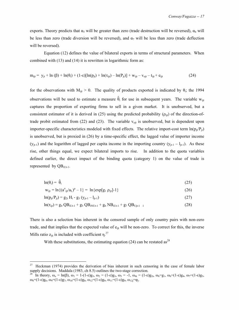
Equation (12) defines the value of bilateral exports in terms of structural parameters. When
combined with (13) and (14) it is rewritten in logarithmic form as:
mijt = yjt + ln (β) + ln(θi) + (1-ε)[ln(pjt) + ln(τijt) – ln(Pjt)] + wijt – vojt – tijt + eijt (24)
for the observations with Mijt > 0. The quality of products exported is indicated by θi; the 1994
observations will be used to estimate a measure θ̂i for use in subsequent years. The variable wijt
captures the proportion of exporting firms to sell in a given market. It is unobserved, but a
consistent estimator of it is derived in (25) using the predicted probability (ρijt) of the direction-of-
trade probit estimated from (22) and (23). The variable vojt is unobserved, but is dependent upon
importer-specific characteristics modeled with fixed effects. The relative import-cost term ln(pjt/Pjt)
is unobserved, but is proxied in (26) by a time-specific effect, the lagged value of importer income
(yjt-1) and the logarithm of lagged per capita income in the importing country (yjt-1 – ljt-1). As these
rise, other things equal, we expect bilateral imports to rise. In addition to the quota variables
defined earlier, the direct impact of the binding quota (category 1) on the value of trade is
represented by QBiUt-1.
ln(θi) = θ̂i (25)
wijt = ln{(aoijt/aL)µ – 1} = ln{exp[g1 ρijt]-1} (26)
ln(pjt/Pjt) = g2t Ht - g3 (yjt-1 – ljt-1) (27)
ln(τijt) = g4 QBiUt-1 + g5 QBiNUt-1 + g6 NBiUt-1 + g7 QBUjt-1 1 (28)
There is also a selection bias inherent in the censored sample of only country pairs with non-zero
trade, and that implies that the expected value of eijt will be non-zero. To correct for this, the inverse
Mills ratio zijt is included with coefficient η.27
With these substitutions, the estimating equation (24) can be restated as28
27 Heckman (1974) provides the derivation of bias inherent in such censoring in the case of female labor supply decisions. Maddala (1983, ch 8.5) outlines the two-stage correction. 28 In theory, ωo = ln(β), ω1 = 1-(1-ε)g3, ω2 = (1-ε)g3, ω3 = -1, ω4t = (1-ε)g2t, ω6=g1, ω6=(1-ε)g4, ω7=(1-ε)g5, ω8=(1-ε)g6, ω9=(1-ε)g7, ω10=(1-ε)g8, ω12=(1-ε)g9, ω11=(1-ε)g9, ω12j=φj.

Conway/Fugazza -- 18
mijt = θ̂i + ω1 yjt-1 + ω2 ljt-1 + ω3 ln(1+tijt ) + Σt ω4t Ht + ln{exp[ω5 ρijt]-1} +
ω6 QBiUt-1 + ω7 QBiNUt-1 + ω8 NBiUt-1 + ω9 QBUjt-1 + Σj ω14jHj + η zijt + eijt (29)
The equations (23) and (29) are simultaneously determined equations. The independent effect of ρijt
in (29) is identified through two channels. First, the cost ratio ĉi that affects the decision to trade in
(16’) does not in theory enter (28) separately from ρijt. Second, ρijt is a non-linear function of the
shared explanatory variables. Equation (28) is itself identified by the inclusion of importer-specific
variables yjt-1 and ljt-1.
IV. Estimation results.
This structural model of bilateral trade in textiles and apparel shares some of the predictions
of the gravity model. The value of bilateral trade will rise with the national income of the importer,
with the share of income spent on this product, and with Δijt. This latter term summarizes the
predictions of greater trade through propinquity, lower transport costs, quality differences, general-
equilibrium effects on prices, and lower policy barriers to trade.
The appearance of Vijt provides a wrinkle to the gravity model stressed by HMR. There is a
possibility of “zeros”: there will be some countries in which none of the firms will be able to export
to country j. 29
The imposition of country-specific quotas will bias bilateral trade in predictable ways. The
value imported from countries with binding quotas will be limited relative to the non-quota
equilibrium, the number of countries exporting to the countries with binding quotas will be at least
as large, and the number of countries served by an exporter subject to a binding quota will be at least
as large as in the non-quota equilibrium. Estimation of the model will allow quantification of these
effects.
The preferred estimation strategy for gravity models has become contested in recent
literature due to the twin problems in these data of country-specific heteroskedasticity and common
zero values. Santos Silva and Tenreyro (2006) propose a Poisson Pseudo-Maximum Likelihood
(PPML) estimator, while Helpman et al. (2008) use a two-step Heckman correction. Martin and
Pham (2009) conduct a comprehensive Monte Carlo test of these and other estimators, and conclude
that when suitable instruments are available for the first and second stage, the Heckman correction is
preferred. We introduce appropriate instruments in the next sections and will follow the two-step
Heckman procedure in estimation.
29 Baranga (2008) provides a different interpretation of the HMR results – one of selection bias driven by defining missing trade values as “zeros” in the data set. This is an interesting direction for future research.

Conway/Fugazza -- 19
The cost ratio from 1994.
Equations (22) through (24) represent equilibrium conditions for the textiles and apparel
markets in each year. To create a benchmark for analysis of adjustment in later years, we estimate
these equilibrium conditions for the pattern of trade observed in 1994 – the last year before the ATC
agreement and the establishment of a schedule for phased removal of quotas.
We estimate the pattern-of-trade equations (22’) and (23’) for 1994 in a random-effects
probit analysis. The exporter-specific cost-quality ratio is estimated directly in this probit through
inclusion of exporter-specific dummy variables. There is an unobserved importer-specific effect to
represent the importer-specific price differential. Distance (Dij), 1994 tariffs (tij94) and shared-border
effects (DBij) are the final determinants.
Tij94 = 1 if and only if ln(aoij94/aL) > 0 (22’)
= 0 otherwise.
ln(aoij94/aL) = αo + α1ln(Dij) + α2ln(1+tij94) + α3DBij + ĉi + α5QBEUit-1
+ α6QBUSit-1 + α7NBQEUt-1 + α8NBQUSit-1 + ζij94 (23’)
with ζij94 = ψj + ωij94
The results of this estimation for textiles and for apparel are reported in Table 4, and the country-
specific estimates for the cost-quality ratio are illustrated in Figure 6.
[Figure 6 about here]
There are two panels to Table 4, reporting alternative techniques for introducing importer-
specific non-quota differences of the pattern-of-trade probit (22’-23’). The top panel reports results
for a fixed-effect estimation and the bottom panel reports results from a random-effects estimation.
Both include fixed exporter effects to derive estimates of ĉi .that are nearly identical; those derived
from the random-effects probit are used as ĉi in what follows. The right two columns report
results from apparel estimation (SITC 841 and SITC 842) while the middle columns report results
for textiles trade (SITC 652). Coefficient estimates are found in the first of each pair of columns,
with the standard errors of coefficients in the second of each pair. The coefficients on the distance
variable are insignificantly different from the theoretical prediction of unity. There is a positive and
significant border effect in textiles trade, while the effect in apparel is positive, smaller, and
insignificantly different from zero. Increased tariffs have the expected negative effect on the pattern
of trade; the effect is significantly larger than zero for textiles and for apparel in the random-effects
estimation, but insignificant in the fixed-effect estimation. Random-effects and fixed-effects
estimation led to nearly identical coefficients on these variables, except the just-mentioned

Conway/Fugazza -- 20
difference in the tariff coefficient, and on the exporter-specific estimates of cost-quality ratio derived
from the two techniques.
The estimates of (the logarithm of) the cost ratio are illustrated in Figure 6. The cost ratios
were rebased through subtraction so that China’s value was zero in both textiles and apparel; the
other countries, as is evident, display values that rise roughly proportionally for both groups of
products. A position above the 45-degree line indicates a relatively lower cost ratio in apparel than
in textiles, while the position below the 45-degree line indicates the reverse. Those countries with
lower cost/quality ratios export to relatively more countries, controlling for distance, adjacency and
tariffs. Hong Kong has the lowest cost indices for both textiles and apparel in 1994, followed by
China, Taiwan and South Korea.30
The exporter-specific quality measure in 1994.
Quality effects are derived for the quota-ridden equilibrium. The equation (29’) is a
restatement of (29) with the quota-liberalization variables excluded. It is estimated for 1994 to
generate the indicators θ̂i of exporter-specific quality.
mijt = θ̂i + ω1 yjt-1 + ω2 ljt-1 + ω3 ln(1+tijt ) + Σt ω4t Ht + ln{exp[ω5 ρijt]-1}
+ Σj ω14jHj + η zijt + eijt (29’)
Table 5 reports the results of this estimation for textiles and apparel trade in 1994. The signs of the
coefficients are for the most part as expected. Importer income increases the value of trade and
distance decreases it, as theory predicts. The tariff coefficient in apparel takes the wrong sign, but is
insignificantly different from zero. The coefficients on firm heterogeneity (μ) and selection bias (φ)
take the correct sign and are both significantly different from zero in textiles; in apparel they have
the correct sign, but only the selection-bias effect is significant. Figure 7 illustrates the distribution
of quality effects by exporting country. The general correlation in effects is positive -- China has
large positive quality coefficients in both textiles and apparel while Mauritania has large negative
coefficients – but by contrast to the cost ratios reported in Figure 6 there is a great deal of country-
specific divergence from the positive diagonal. Vietnam and Niger, for example, have quite similar
30 The most efficient countries are an interesting mix of Asian emerging economies and developed-country producers. Among the ten most efficient countries are China, Taiwan, Hong Kong, Korea, India and Pakistan from the Asian emerging economies, as well as USA, Germany, Great Britain and Japan. The least-efficient producers are least-developed economies from the Caribbean, Africa and the Middle East.

Conway/Fugazza -- 21
quality estimates in textiles. At the same time, Vietnam is among the highest-quality exporters of
apparel and Niger is among the lowest-quality exporters.31
[Figure 7 around here]
Testing the hypothesis using the post-quota years: 2005 and 2006.
Estimation of the three-equation system (22), (23) and (29) for bilateral trade in the years
2005 and 2006 provides the clearest test for the existence of trade creation, trade diversion, trade
deflection and trade destruction. In Table 6 we report the results of this estimation for bilateral
textiles and apparel trade in these two years. Coefficient estimates are reported in the first line, with
standard errors in parentheses beneath each. Exporter-specific effects are estimated, as theory
suggests, but are not reported here.
The pattern-of-trade probit estimation in the first column uncovers a structure similar to that
predicted. The distance effect is significant and has a coefficient close to -1. The probability of
positive exports to a country is increased significantly by sharing a border. Importing countries with
higher tariffs are significantly less likely to trade with an exporter, on average. The cost-quality ratio
derived for 1994 proves to be a significant predictor for trade in 2005/2006. The coefficient value of
-1.49, significantly less than -1, indicates that the pattern of trade in 2005/2006 is significantly more
unbalanced than in 1994 – countries with low cost-quality ratios expanded their exports to new
countries more than proportionately, while countries with high-cost quality ratios exported to
disproportionately fewer trading partners – even after controlling for the effects of quotas. Further,
countries were likely to export to significantly more countries in 2006 than in 2005, as indicated by
the 0.11 coefficient on the year indicator T2006.
The quota effects proved to be insignificant in large part for the pattern of textiles trade. The
trade diversion effect (NBiUt-1) takes the wrong sign, but is insignificantly different from zero. The
trade deflection effect (QBiNt-1) is negative, as predicted, but also insignificantly different from zero.
The trade destruction effect (QBUjt-1), by contrast, is positive as predicted and significant – countries
that were subject to binding quotas in 1994 are by 2005/2006 importing textiles from significantly
more trading partners than are countries not subject to binding quotas in 1994.
The value-of-trade equation for textiles is reported in the second column, and also reflects
the structure predicted by theory. The distance effect is negative and insignificantly different from -
1, as is typical of gravity models. The importer-tariff effect is negative, significantly different from
31 The exporters with highest quality are not surprisingly very similar to the group with lowest cost/quality ratio: Asian emerging economies (China, Hong Kong, Taiwan, Korea, India) and industrial economies (US, Italy, France) are among those with high quality in both products, while Burkina Faso, Mauritania and Ugana are found at the other end of the distribution.
Conway/Fugazza -- 22
zero, and with tariff elasticity of demand equal to -3.12. Income and population importer effects are
positive and significant. The coefficient on population is surprisingly large, but perhaps reflects the
need for labor-abundant countries to import textiles so that apparel can be exported. The
heterogeneous-firm (μ) and selection-bias (η) corrections are significant and take the expected
positive sign. For 2006, the average bilateral import value was significantly less than the amount
observed in 2005.
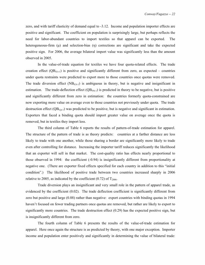
In the value-of-trade equation for textiles we have four quota-related effects. The trade
creation effect (QBiUt-1) is positive and significantly different from zero, as expected – countries
under quota restraints were predicted to export more to those countries once quotas were removed.
The trade diversion effect (NBiUt-1) is ambiguous in theory, but is negative and insignificant in
estimation. The trade-deflection effect (QBiNt-1) is predicted in theory to be negative, but is positive
and significantly different from zero in estimation: the countries formerly quota-constrained are
now exporting more value on average even to those countries not previously under quota. The trade
destruction effect (QBUjt-1) was predicted to be positive, but is negative and significant in estimation.
Exporters that faced a binding quota should import greater value on average once the quota is
removed, but in textiles they import less.
The third column of Table 6 reports the results of pattern-of-trade estimation for apparel.
The structure of the pattern of trade is as theory predicts: countries at a farther distance are less
likely to trade with one another, while those sharing a border are significantly more likely to trade
even after controlling for distance. Increasing the importer tariff reduces significantly the likelihood
that an exporter will sell in that market. The cost-quality ratio has effects nearly proportional to
those observed in 1994: the coefficient (-0.94) is insignificantly different from proportionality at
negative one. (There are exporter fixed effects specified for each country in addition to this “initial
condition”.) The likelihood of positive trade between two countries increased sharply in 2006
relative to 2005, as indicated by the coefficient (0.72) of T2006.
Trade diversion plays an insignificant and very small role in the pattern of apparel trade, as
evidenced by the coefficient (0.02). The trade deflection coefficient is significantly different from
zero but positive and large (0.88) rather than negative: export countries with binding quotas in 1994
haven’t focused on fewer trading partners once quotas are removed, but rather are likely to export to
significantly more countries. The trade destruction effect (0.29) has the expected positive sign, but
is insignificantly different from zero.
The fourth column of Table 6 presents the results of the value-of-trade estimation for
apparel. Here once again the structure is as predicted by theory, with one major exception. Importer
income and population enter positively and significantly in determining the value of bilateral trade:

Conway/Fugazza -- 23
in this case, the population coefficient (0.08) reflects a smaller effect of population on trade value
than was observed for textiles. Higher importer tariffs reduce trade values significantly, and with
similar large (-3.04) coefficient. The firm-heterogeneity term and the selection-bias correction both
enter with positive and significant coefficients, as predicted. The contradiction to theory comes in
the distance coefficient; at (0.35) it is positive, though insignificantly different from zero. The
average value of bilateral trade in 2006 was significantly reduced from 2005, in striking contrast to
the increase in the propensity to trade noted above.
The quota effects on the value of apparel trade are large and significant. The trade creation
effect of removing the quota (1.85) is large, positive and significant. The trade deflection effect (-
3.32) is large, negative and significant: countries with binding quotas in 1994 have greatly reduced
the average export value to third countries in 2005-2006. The trade diversion effect (0.36) is
positive and significant, contrary to theory – countries not under quota in 1994 have expanded their
average export value to the quota-levying countries in 2005-2006. Trade destruction also does not
work as predicted: countries facing binding quotas in 1994 are importing significantly smaller
values (-1.13) of apparel on average from trading partners than in 1994. This last effect is observed
as well in textiles.
The evolution of trade from 1994 to 2005/2006 can be decomposed into three systematic
sources: the structure of trade, the impact of quotas, and exporter-specific adjustments. The first
two are analyzed above,
Measuring the relative contribution: a decomposition.
Let’s consider the difference between post-quota and during-quota outcomes in the value of
bilateral trade. We can represent the change in bilateral values as follows:
ΔMijt = ψ ΔXijt + Xijt Δψ + ω ΔQijt + Δ ζj + Δζi + ξijt (30)
where Xijt represents the exogenous variables determining the value of trade, and ψ represents the
during-quota coefficients associated with those exogenous variables. Table 5 reports the exogenous
variables and coefficient estimates that Xijt and ψ represent. There are thus six potential sources of
the observed change in bilateral values:
Changes in the determinants of bilateral trade (as represented by ΔXijt);
Changes in the intensity of response to determinants (as represented by Δψ);
Changes in the quota regime (ΔQijt);
Changes in importer behavior (Δζj);

Conway/Fugazza -- 24
Changes in exporter behavior (Δζi);
Random shocks and otherwise unmodeled changes (ξijt).
A similar decomposition is possible for the propensity to trade between any two countries.
Examining the evolution of trade by dividing the sample.
While the end of the quota system began in principle with the 1995 ATC agreement, the
bulk of the liberalization that occurred was observed in the period from 2002 to 2005. In this section
we estimate the pattern and value equations for the two subperiods 1995-2001 and 2002-2006 to
uncover any differences in the structure of bilateral trade.
Table 7 reports the results of estimation of the pattern of trade (equations (22) and (23)) in
these subperiods. For textiles (second and third column) the non-quota coefficients take the
expected signs, but do differ significantly from earlier to later sample. The negative effect of
distance on the propensity to export remains significant and close to negative one. The increased
propensity to export to neighboring countries increases significantly from the earlier to the later
period. There is a magnification effect of quality-adjusted cost advantage, and this magnification
increases in the 2002-2006 period. The negative impact of increasing importer tariffs on the
propensity to export is significantly larger in the later period. The time dummy variables are
measured relative to the excluded period (2001 and 2006, respectively). There was a “bubble” in
propensity to export in the earlier period, with propensities highest in 1999 and 2000. After 2001,
the propensity to export rose monotonically from 2002 through 2006.
The country-specific effects of quota liberalization in textiles are evident in the 1995-2001
period, but not in the 2002-2006 period when quota liberalization was more widespread. The trade
deflection effect is positive (at 0.12), statistically significant and runs counter to theory: removing
binding quotas from an exporter is associated with an increase in the propensity to export to other
countries. The trade diversion effect is negative (-0.15), significant and as expected: countries who
were not bound with quotas in the earlier period will experience a lower propensity to export once
the quotas are no longer binding. The trade-destruction effect is positive (0.39), statistically
significant and of expected sign: exporters whose binding quota is removed will have a propensity
to import from more trading partners. The coefficients corresponding to these effects are all
insignificant and smaller in magnitude for the 2002-2006 period.
The results for the pattern of bilateral trade in apparel are reported in columns four and five.
The effects of distance are once again significant, but are significantly less than -1.0: distance is less
Conway/Fugazza -- 25
of an impediment to trade in apparel than in textiles. There is once again an increased propensity to
export for countries that are neighbors, and that effect becomes more pronounced in the more
liberalized period. The impact of increased importer tariffs on the propensity to trade is negative but
insignificant during the quota period, and a stronger, significant negative effect during the more
liberalized period. In contrast to the textiles example, the quality-adjusted cost advantage does not
reflect the magnification effect in the earlier period. This effect becomes more negative in the later
period, and in fact indicates (with coefficient -1.00) that the conditions observed in 1994 in terms of
propensity to export are in fact replicated in the more liberalized period once quota, time and
country-specific effects have been controlled for. In the earlier period, the largest average
propensity to export was observed in 1996, with a dip in 1997-199 and a recover in 2000; in the later
period, the average propensity to export grew monotonically from 2002 to 2006. The rise in
propensity to export was relatively largest in 2006, similar in pattern to textiles, although the rise in
propensity was relatively larger in apparel.
The bilateral trade propensity effects of removing binding quotas in apparel are similar to
those observed in textiles. Considering first the earlier period, relaxing quotas was associated with
exports to more countries, rather than fewer, once again counter to theory. The trade diversion effect
was negative, significant, and larger (-0.48) in apparel: once quotas are relaxed, those countries not
subject to quotas had lower propensity to export on average. The trade destruction effect was
positive as in textiles though in this case insignificantly different from zero. For the 2002-2006
period the trade deflection effect became insignificant, but the trade diversion effect on propensity to
export remained significant and negative. The trade destruction effect was positive and significantly
different from zero in the 2002-2006 period.
Table 8 reports the determinants of the average bilateral value of trade (equation (29)). The
results for textiles (second and third columns) are once again consistent with theory. The average
value of textiles exports rises significantly with rising income and population of the importing
country, with larger effect attributable to population. (This is probably due to the nature of textiles
as an imported input to labor-intensive apparel manufactures.) The population effect is significantly
larger in the later period. The negative effect of rising importer tariffs on the average value of
exports is significant, and is not significantly different in the later from former period. The
coefficient μ of the distribution of domestic producers is significant in both subperiods, but is not
changing significantly from one period to the next. The selection-bias coefficient η is positive and
significant, as expected, but is significantly smaller in size in the later period.
The value of bilateral trade in apparel (fourth and fifth columns) is also largely stable in its
non-quota determinants. The effects of importer income and population are quite similar in the two
Conway/Fugazza -- 26
periods, but the weight of the two is reversed when compared to textiles. Importer income has a
larger elasticity (0.20) while the elasticity of bilateral value with respect to population is smaller
(0.06) while still significantly different from zero. The elasticity of bilateral trade value with respect
to importer tariff is negative, large (-6.01) and significant in 1995-2001; while the elasticity falls in
absolute value in 2002-2006, it remains quite large. The effect of distance on value of bilateral
exports is positive for apparel in 1995-2001, changing to a negative but insignificant value in 2002-
2006. The firm-heterogeneity effect μ is large (1.95), significant, and little changed from earlier to
later period. The selection-bias term φ is insignificantly different from zero in the earlier period, but
becomes larger (0.52) and significantly different from zero in the period of quota liberalization. The
average value of bilateral exports fell between 1995 and 2000. After a partial recovery in 2001, the
average value fell monotonically from then through 2006.
The effects of relaxing quotas in textiles in the 1995-2001 period are significant, but take the
opposite sign from those for the pattern of trade. There is first of all the relative increase in exports
by the quota-bound exporter once the quotas for that importer are relaxed: this is positive (0.48),
large and significantly different from zero. The trade-deflection effect is negative (-0.28) and
significantly different from zero: the bilateral value of exports to other importers on average by a
quota-bound exporter is reduced as the quota is relaxed. This is consistent with theory. Trade
diversion effects are significant in 1995-2001 but positive (0.10): relaxation of a quota on one
exporter is associated with increase on average in bilateral exports from other (non-bound) exporters.
The trade destruction effect is negative (-0.43) and significant, contrary to theory. The effects of
relaxing quotas in apparel take the same signs as those for textiles, but are larger in magnitude and
remain significantly different from zero. While the trade creation effect is larger in the quota-
liberalization period 2002-2006, the trade-diversion, trade-deflection and trade-destruction effects
are smaller in magnitude.
The role of quotas.
The measures of quota relaxation that we use allow us to identify the behavior of that group
of countries with binding quotas in 1994. We characterize the trade of that group completely: QBiUt
captures the effect of quota relaxation on exports to the quota-setting country, QBiNt captures the
effect on exports by this group to countries not levying the quota, and QBUit captures the impact of
quota relaxation on the imports (from all countries) of the goods under consideration. Following
theory, we also consider the impact of quota relaxation on the exports to quota-setting countries
(NBiUt) by exporters not subject to binding quotas. Estimation results suggest the following
conclusions about the direct effects of quota liberalization:

Conway/Fugazza -- 27
There is evidence of trade creation with the relaxation of quotas: the coefficient on QBiUt-1
in the value-of-trade equation is invariably positive and significantly different from zero.
There is evidence of the elimination of trade diversion. The coefficient on NBiUt-1 in the
pattern-of-trade equation is negative while the coefficient in the value-of-trade equation is
positive. Fewer countries not previously subject to binding quotas have exported to the
quota-setting countries on average with liberalization, while those that continue to export are
selling larger values on average into the formerly quota-constrained markets.
The expected effects of trade deflection are not in evidence. Theory predicts that countries
subject to binding quotas will sell into third markets, but that behavior will be reversed once
quotas are removed. In fact, the coefficients on QBiNt-1 indicate that the removal of quotas is
associated with an increased propensity by these countries to export into third markets, and
that the average value of exports into those markets is reduced.
There is evidence that trade destruction is reversed with relaxation of quotas. Those
countries with binding quotas in 1994, indicated by QBUit-1, experienced a significantly
increased propensity to import with the relaxation of quotas. The average value of bilateral
imports declined significantly.
These are statistically significant effects, but they represent a small contribution to the overall shift
in the pattern and value of trade. The countries subject to binding quotas play an important role in
the evolution of the world market, but it is the changes in bilateral trade among those countries not
subject to or imposing binding quotas that define the stylized facts outlined in the introduction.
The role of country-specific factors.
Exporter-specific adjustments are evident in the exporter fixed effects from both pattern- and
value-of-trade estimation for the estimation of Table 6, and these tell a nuanced story of the
adjustment of exporters to the liberalization of quotas. Figure 8 illustrates the exporter-specific
effects for textiles: the horizontal axis indicates for each country the exporter-specific effect on the
pattern of trade, while the vertical axis indicates the exporter-specific effect on the average bilateral
value of trade. The fixed effects are “normalized”, with the mean fixed effect subtracted from each
observation and the coefficient standard error dividing the difference. The coefficient values thus
represent an approximate test of significant difference from the mean. An underlying coefficient
more than 2 standard deviations from the mean will have “normalized” value greater than 2 in
absolute value.
[Figure 8 about here]

Conway/Fugazza -- 28
Exporters in the upper-right quadrant are exporters that have increased the number of trading
partners in both textiles and apparel between 1994 and 2005/2006 after controlling for structural
changes and the liberalization of the quota. This group of countries does not include those usually
associated with comparative advantage in textiles and apparel trade, but rather African, Eastern
European and Latin American countries such as Seychelles, Georgia, Mauritania, Bahrain and
Nicaragua. The lower-left quadrant includes those exporters that, after controlling for the structure
and quota effects, have both low propensity to export and low average bilateral trade value relative
to the mean serve. This is a mixed group, with African countries such as Malawi and Mozambique
as well as Kyrgyz Republic, Argentina and Ireland. The upper-left quadrant includes exporters (after
controlling for structural and quota differences) with below-average propensity to export and above-
average bilateral export value: Belarus, Turkey, Sri Lanka, as well as Finland, Austria, Canada and
Spain. The lower-right quadrant includes exporters with an above-average propensity to export but
below-average bilateral trade value: many African (e.g., Senegal, Benin, Tanzania, Kenya),
transition (Mongolia, Azerbaijan, Armenia) and other (Nepal, Uruguay) exporting countries. Given
the scaling, we can see that few of the observations on the relative value of trade are significantly
different from the mean. The exporting countries differ significantly with regard to the pattern of
trade, however, with traditional exporters (China, Korea, Indonesia, Taiwan) grouped with
developed countries (US, Japan, Great Britain, France) with propensity to export significantly lower
than the mean while a large group of small exporters (Nicaragua, Bahrain, Senegal, Nepal, Estonia,
Uganda, Slovenia) have propensities to export significantly above the mean.
Figure 9 reports similar statistics for the country-specific effects in apparel. In this case, the
value-of-trade statistics are in every case less than two standard deviations from the mean, while
once again a large group of countries have propensities to export significantly different than the
mean. The countries for which both propensity to export and average bilateral value of trade fell
include most of the quota-imposing countries ( for example US, Great Britain, Germany, Italy,
Austria, Netherlands, Canada) as well as Japan, New Zealand and Moldova. Those exporters above
average in both dimensions include Moldova, Uganda, Georgia, Seychelles, Mauritania, and Kyrgyz
Republic. Those for which there is a tendency to “focus” trade (falling propensity to export coupled
with larger average bilateral trade values) include most of the traditional exporters (China, India,
Hong Kong, Korea, Malaysia, Pakistan), but also Bahrain, Jamaica, Hungary, Qatar, Guatemala and
Mauritius. The final quadrant includes countries that have a tendency to diversity trade: above-
average propensity to export coupled with a reduced average bilateral trade value. This group is a
mix of developed countries (France, Australia, Norway) with countries that have become export

Conway/Fugazza -- 29
platforms to the US and EU: Lithuania, Latvia, Ukraine, Nicaragua, Croatia, Slovak Republic,
Jordan, Morocco, El Salvador.
[Figure 9 about here]
Figures 8 and 9 provide a cross-sectional picture of the country-specific effects for 2005-
2006. We obtain a more dynamic picture by using the exporter-specific effects from the estimation
results in Tables 7 and 8. Figure 10 plots the country-specific effects derived from the propensity-
to-export estimation for textiles for the two periods 1995-2001 and 2002-2006. These effects reflect
the country-specific propensity to export in the two periods once the common, quota and time effects
of Table 7 have been controlled for. The observations in each period are rebased by subtraction of
the average country effect for the sample, but are not divided by standard deviation – they remain in
comparable units of “propensity to export”. The heavy black line represents the 45o line: if there
were no change in relative country-specific propensity to export from the earlier to the later period,
the country-specific scatter of points would all fall on that line. As is evident, this is not the case.
Countries with above-average propensity to export in the 1995-2001 period on average experienced
an even-greater propensity to export in 2002-2006; those with below-average propensity to export in
1995-2001 experienced an even larger drop in relative propensity. Figure 11 illustrates the
analogous scatter of country-specific effects for the propensity to export apparel derived
simultaneously with the coefficients of Table 7, with the same pattern of increased propensity to
export of “above-average” countries and reduced propensity to export of those countries initially
“below average”.
[Figure 10 about here]
[Figure 11 about here]
We can interpret the negative and positive values as below-average performance and above-
average performance, respectively. After controlling for the exporters’ natural and quota-induced
advantages, how well did they do? The concentration of observations above the 45o line in the first
quadrant and below the 45o line in the fourth quadrant indicates that quota liberalization on average
made this pattern of over- and underperformance even stronger. The lower quadrant on the two
figures is populated by many of the same countries. The developed countries (e.g. US, Japan,
Germany, Great Britain, France) are uniformly in this quadrant: given their advantages, they are
below average in propensity to export. Many Asian exporters (e.g. Hong Kong, Korea, Singapore,
Taiwan, Thailand) are also found there: in fact, China is among the countries in the fourth quadrant
below the line. This indicates that once the common advantages that China shares and the
liberalization of quotas are considered, China could have been expected to perform better in reaching

Conway/Fugazza -- 30
new markets.32 The countries that were above average differ by market. Nicaragua, Algeria,
Mauritania, Senegal, Grenada, Uganda and Nepal were highest-ranked in textiles in 1995-2001, and
this advantage was magnified in 2002-2006. Eastern European countries (Moldova, Latvia,
Lithuania, Ukraine, Armenia, Croatia) as well as Kyrgyz Republic, Nicaragua, Ghana, and Uganda
were the highest performers in 1995-2001 in apparel, and these countries experienced an
intensification of that performance in 2002-2006.
Figures 12 and 13 describe country-specific achievement in terms of average bilateral value
of exports for textiles and apparel, respectively. In Figure 12 we observe an evident preponderance
of observations in the first and fourth quadrants for textiles, though there are more outliers from that
than in the propensity to export and there is less evidence of a magnification effect. Those below
average in terms of value of bilateral trade tend to be developing countries (Mozambique, Benin,
Guyana, Burundi, Malawi, Kyrgyz Republic, Argentina, Honduras), although the US also falls into
this category. Those above average in both earlier and later periods (Bahrain, Grenada, Mauritania,
Bangladesh, Vietnam, Philippines) are a mix of new and traditional textiles exporters. China, India
and Singapore are found among the many countries near the origin – once common advantages are
controlled for, the countries do not stand out in terms of average value of bilateral export. Figure 13
illustrates the average value of exports in apparel. There is much less of a pattern here. It is still
the case that those with high country-specific effect in 1995-2001 will have positive country-specific
effect in 2002-2006, but the magnification of the previous figures is absent here. It is here, in this
figure, that the outlying performance of China becomes evident. The vertical distance of each point
above the 45o line can be thought of as the country-specific improvement in average value of
bilateral exports from the 1995-2001 period to the quota liberalization period of 2002-2006. China
stands alone by this measure. At the opposite extreme are countries with a decided disadvantage in
apparel trade: Yemen, Zimbabwe, Sudan, and Central African Republic among others.
The China effect.
China and its capacity for exporting textiles and apparel occupy a central position in any
debate over global adjustment to removal of quotas. As Conway (2010) reports, China’s share (in
value terms) of the combined US and EU markets for textiles and apparel rose from 18 percent in
2001 to nearly 34 percent in 2008. The preceding discussion marked significant difference of China
from the other countries with binding quotas in 1994 only in the growth in average apparel exports
32 For some countries like China, Italy or the US, there is also the “universe” effect to consider. These countries were already exporting to most of the other countries in the sample. There was less scope for expansion in terms of reaching new markets that for countries beginning with many fewer trading partners.
Conway/Fugazza -- 31
between 1995-2001 and 2002-2006. In this section we redo the estimation strategy of the earlier
section over the subsample of bilateral observations that include China as exporter or importer.
V. Linking the two sectors.
The preceding analysis was undertaken with the assumption that the textiles and apparel
industries were independent. In fact, they are closely linked along two dimensions. First is the
technological dimension: because the two industries developed together and are two stages in a final
product, it is to be expected that countries with comparative advantage in production of textiles will
(other things equal) have existing production of apparel. Second is the dimension of regional
integration: if a country has comparative advantage in production of textiles, it will look for regional
partners to process the textiles into apparel for re-export to the country of origin of the textiles. Each
of these is investigated in turn in this section.
Given that the textiles sector is the upstream sector in this linkage, analysis of that sector is
unchanged. The probit estimation for textiles is used to create two fitted values in predicting trade
flows: ŝijt is the prediction that country i will export textiles to country j, while ŝjit is the prediction
that country i will import textiles from country j. The ŝijt variable will pick up the common-cost
advantage of a textiles producer (or economies of scope): if a country has a natural comparative
advantage in both, or there are economies of scope, then positive ŝijt will be correlated positively
with export of apparel. The coefficient of ŝjit will take a positive value when there is evidence that
textiles exporters more often sell to importers using the textiles for offshore assembly and re-import
of apparel to the textile-exporting country.
The specifications in Table 15 extend the structure of Table 14 to include the variables ŝijt
and ŝjit. For countries predicted to be textile exporters to country j in period t, the value of apparel
exports to country j is also significantly more – this is consistent either with an argument of common
comparative advantage in the two sectors or in an argument of economies of scope in internalizing
textiles and apparel production within the same supplier. An increase in the probability of textiles
export from country i to country j tends to increase the mean value of apparel exports from i to j by
1.77 percent in specification (4). An increase in the probability of textiles export from country i to
country j also increases significantly the mean value of apparel exports from j to i, by a nearly 0.70
percent. This is an indicator of “offshoring”. Specification (4) is the closest to the theoretical
specification. Importer GDP and population effects are significant and take the expected sign.
Importer tariff also has a strongly negative effect on the mean value of imports. The inverse Mills
ratio takes the coefficient η=3.243. The quota spillover effects are also similar to those reported
Conway/Fugazza -- 32
above. The supplier heterogeneity effect μ = 1.983 is significantly different from zero and similar to
that of Table 14.
When we consider the coefficients linking textiles and apparel, both are significantly
different from zero in the last three specifications. In these specifications we see large jumps in the
“economies of scope” effect but relative stability of the “offshoring” effect. For the “offshoring”
effect proxied by ŝjit, the elasticity falls in the range (0.7-1.03). For the “economies of scope” effect
proxied by ŝijt, the elasticity falls in the wider range (1.77-2.6).
VI. Predicting the effect of removing quota restrictions.
Since 2005 marks the end of the quota system, theory predicts that the pattern of trade in
these two categories will become more focused: fewer countries will export to those countries
formerly under quota (less trade diversion), and those exporters serving the formerly quota-
restrained countries will export to fewer other countries (less trade deflection). This is not
immediately evident in the data, as Table 16 illustrates. For these 125 countries, there are 201500
observations of bilateral imports over the thirteen-year sample. If the share of bilateral observations
with non-zero trade is calculated for each year, it is evident that in both textiles and apparel there has
been a diversification in trading patterns. The share of possible bilateral pairs with non-zero textiles
imports was 19.3 percent in 1994; by 2004 it was 24.5 percent. In apparel, the similar calculation
yields 31 percent in 1994 and 39.1 percent in 2004. This increased share is consistent with steadily
increasing trade diversion and trade deflection from an increasingly binding system of quotas.
This explanation is less compelling, though, for 2005. With the removal of quota
restrictions, other things equal, we predict a fall in this percentage. Instead, there is a jump in both
shares larger than observed in previous years. These shares are unconditional means, and as such do
not reflect the impact of other possible determinants. To address this question properly, we
undertake a comparative-static exercise based upon the estimation results of the previous sections.
First we examine the estimated impact of quota restrictions from the data panel for the
quota-driven period 1994-2004. The coefficients are derived in the earlier section and are
reproduced in Table 17. The first two columns represent the effect of the quota on the observed
pattern of trade, while the last two columns represent the effect of the quota on the mean value of
imports given that trade occurs. These coefficients are taken from the theoretically consistent
regressions (right-hand column) of each table. The observed pattern of trade in textiles is not
significantly affected by the existence of quota limits, but there is a significant effect of binding

Conway/Fugazza -- 33
quotas on the pattern of trade.33 Theory suggests that these coefficients will be positive – a quota
limit or binding quota will encourage the exporter to develop new export markets. The econometric
results support that conclusion in three cases out of four. In textiles the country with binding quota
of the EU will other things equal, have a significant higher probability to export to the average
importer. Such an effect does not exist for a country with binding quota of the US. In apparel, a
binding quota whether in the US or the EU has the expected effect of increasing the probability of
exporting to an average importer. The size of the effect is the largest with a binding quota in the EU.
The effects of quotas limits on the average value of exports by the country under quota can
be broken into the impact on the quota-setting country and on other countries. The quota limits,
whether by US or EU, are associated with significantly larger mean-value exports to the quota-
setting country, other things equal. The effect on the mean export value to other countries is positive
with the EU and negative with the US. Consider the example of the US: quota limits on an apparel
exporter are associated with a significantly larger import by the US from that country (4.68) but
minimal and insignificant effect on imports by other countries (-0.007). Quota limits on a textiles
exporter are also associated with significantly positive change in mean value of US imports from
that exporter (2.557), but negative and significant effect on mean value of exports of that country to
non-US importers (-0.141). The causality here should probably be reversed – exporting countries
are given quota limits when they demonstrate the ability to export large amounts to the US (or EU).
Binding quotas have significant additional effect to quota limits for the quota-setting country: for
the US, 1.743 and 1.263 for apparel and textiles respectively. The effect of these binding quotas on
mean value of exports to non-quota-setting countries is always significant for both EU and US
quotas but with no clear-cut pattern. It is positive for the US in textiles and the EU in apparel and
negative for the US in apparel and the EU in textiles. The EU results are possibly influenced by the
fact that eastern acceding countries have not been treated as EU countries in the sample but have
shown (see Table 4) a clear improvement in their production efficiency in apparel.
For a second investigation of the impact of quotas, we use out-of-sample forecasting to
check actual against predicted patterns of trade. We begin from the quota-distorted equilibrium of
1994-2004 as summarized in the probit regression results of Tables 9 and 10 and the non-linear
regression results of Tables 13 and 14. We then use these results to forecast the trade pattern and
trade volume in 2005. Tables 19 summarize our results for the trade pattern. These out-of-sample
forecasts were calibrated on the 1994-2004 data, and in this table the estimated probability used to
separate predicted trade from no predicted trade was chosen to ensure equal numbers of Type 1 and
33 The coefficients on quota limits are not reported, just as in the preceding tables, but augmented probits including those quota limits led to insignificant coefficients on those variables.
Conway/Fugazza -- 34
Type 2 errors (Actual: no; Predicted: yes – or Actual: yes; predicted: no) in that sample. As is
evident in Tables 19, the model’s predictions for both 2005 and 2006 are significantly skewed
toward Type 2 (Actual: yes; predicted: no) errors both for textiles and for apparel: we have observed
greater numbers of bilateral trading combinations. Just as is evident in Table 17, this exercise
indicates that 2005-2006 was a period of diversifying trade unpredicted by the simple model of
Vinerian trade creation. The hypothesis that removal of quotas will lead to greater trade focus – i.e.,
less trade diversion and less trade deflection – does not hold in aggregate for neither 2005 nor 2006,
even when controlling for other factors that might affect trade patterns.
Tables 20 compare bilateral mean export value and number of export markets on average in
1994-2004 to 2005 and, 2005 to 2006 for each exporter. The country acronyms in bold in these two
tables are the countries subject to binding quotas in 2004. The Vinerian prediction was to observe
the quota-bound countries in the lower left-hand corner: increased mean export value and reduced
number of export markets. In Table 20a, the results for textiles trade in 2005 indicate that this is the
case for India, Korea, Pakistan and Thailand but not for Belarus, China and Malaysia. The latter
three countries have seen their mean export value increase together with the number of export
destinations. The combination of increased mean export value and increased number of export
markets is the most-often observed (95 countries out of 125). In 2006, the Vinerian pattern remains
only for Korea and emerges for Malaysia.
Table 20b illustrates a similar pattern for bilateral trade in apparel. The pattern of this is suggestive
– a binding quota in 2004 is associated with a reduced number of export markets in 2005 in 10 out of
14 cases, as the Vinerian hypothesis suggests. The majority of countries, though, are associated with
an increased number of export markets in both 2005 and 2006. The mean value of exports tends to
increase for most countries in 2005 but falls in 2006 with respect to 2005. This suggests that
countries do find fewer purchasers in the US and EU markets post-quota; their producers then adjust
by selling less to a greater number of other importers. We also have countries appearing to be
negatively hurt by the removal of the quotas including three countries with a binding quota in 2004,
namely India, Indonesia and Singapour.
Comparing actual and predicted for 2005, as done here, leaves open three possibilities for
the source of the change. First, the removal of the quota system may have triggered the effect.
Second, there could have been a change to the common costs of or benefits from bilateral trade that
led to a change in “normal” trade. Third, there could have been country-specific idiosyncratic
effects that caused the divergence. The analysis preceding this combined these three possibilities.
We examine the evidence of the second effect by measuring the change in coefficients of the probit
Conway/Fugazza -- 35
and regression equations when 1995-2004 and 2005-2006 are compared. Table 21 reports these
results.
The coefficients reported in (1) columns of Table 21 are the coefficients on the explanatory
variables estimated in the 1994-2004 analysis reported earlier in columns (3). Columns (2) contain
coefficient estimates obtained for specifications without quota dummies and without selection and
productivity controls in the value of trade estimation sets. Columns (3) show the coefficients when a
similar to columns (2) analysis is done for 2005-2006 alone. Significant differences would indicate
a fundamental change in the “normal” pattern and value of trade as defined in earlier sections.
No dramatic changes can be found in the determinants of the pattern of trade, except for tariffs in
apparel and the existence of a common border in textiles. Both changes however affect positively the
trade pattern. Tariffs appear to be less of an obstacle and the premium to contiguity increases.
As to the value of trade, differences across columns (2) and (3) would indicate an overall structural
change. We observe that the economic size of the importing country (ln(Yjt-1), ln(Ljt-1))
predominantly played a significantly larger role in increasing the mean value of trade in 2005-2006
in both textiles and apparel. This is not the case for distance whose coefficient is larger for the 2005-
2006 in both sectors. The change in the coefficient on average tariff (1+tjt) indicates that tariffs took
on a larger discouraging effect on the mean value of trade in 2005-2006 in textiles but a smaller one
in apparel. The quality of the export goods (ĉi) became a larger determinant of the value of trade in
textiles but not in apparel. There probably was a “flight to quality” in textiles in 2005-2006 when
countries were no longer constrained by quotas. In apparel, exporters may focus on quality-driven
product differentiation and competitiveness.
VII. Conclusions and extensions.
The global story of the removal of quotas on textiles and apparel has been told in large part
from the perspective of the quota-setting countries, and in particular the US and the members of the
EU. This paper nests that perspective within the global fabric of trade. The removal of the ATC
quotas in 2005 served as a shock to which all trading countries must adjust – not just the consumers
in the US and EU. The conclusion of this paper supports the Vinerian trade creation story, but with
a twist. While the countries presumed to be comparative-advantage exporters of textiles and apparel
exhibit the expected increased exports to the quota-removing importers, the other exporters whose
market has been reduced in the US and EU have expanded their exports to larger numbers of smaller
importers than they served during the quota period.
The model presented here proves to be effective in capturing both the pattern and value of
international trade in textiles and apparel, and may be useful in other industry-level trade studies. It

Conway/Fugazza -- 36
introduces a number of improvements over the typical gravity-equation or CGE model. First, it
identifies the comparative-cost advantage of exporting countries by looking across importers, rather
than simply at the US or European market. Second, it incorporates the heterogeneity of suppliers
within the exporting country; this proves to be an important factor in explaining the variation of
export success by the same country across trading partners. Third, it introduces the impact of the
ATC system of bilateral quotas imposed by the US, EU and Canada during this period. Fourth, it
endogenizes the export-platform explanation for offshoring.
The heterogeneity of suppliers within an exporting economy is advanced in Melitz (2002)
and HMR as a useful way to consider the incremental nature of exporter response to export
incentives. This proves its worth in the present analysis. The pattern of trade provides us with an
insight into that heterogeneity that can be exploited and then applied to distinguish the impact of the
quota regime.
The deflection effect of quotas on other importers is evident in the data. First, quotas in the
US and EU are associated with exports to more non-quota destinations, even after controlling for
importer size, distance, tariffs and other features of the economies. Second, there is evidence that
binding apparel quotas in the US are associated with increased apparel exports by those constrained
exporters in other countries.
There is strong support in the data for the export-platform argument. If country j exports
textiles to country k, then the value of apparel exports from k to j is significantly increased.
Use of the model for out-of-sample forecasts of textiles and apparel exports in 2005 suggests
a reality that is more complex than the simple prediction that “China takes over the market”. The
year 2005 was not characterized overall by the “focusing” of the pattern of trade suggested by the
simple predictions of CGE models – there was in fact an increased diversification of trading patterns
over the quota-restricted periods on average. There was also a reduction in the average trading
volume of both exporters and importers during 2005, but this was a continuation of a trend evident in
the data in previous years.
The technique used here has not only identified the “normal” trade pattern and mean value
of trade, but has also identified countries that stand out in their success in dealing with the removal
of the ATC quotas. In examining Tables 17 and 18, for example, we note the success of Turkey and
Pakistan in both expanding the number of importers for its textiles and apparel and expanding the
mean value of shipments to those importers. It will be useful to investigate these successful
countries more closely, specifically in the context of the heterogeneous supplier framework put
forward by HMR. This can be done through analysis of plant-level decision-making.

Conway/Fugazza -- 37

Conway/Fugazza -- 38
Biography. Anderson, J.: “A Theoretic Foundation for the Gravity Equation”, American Economic Review 69, 1979, pp. 106-116. Anderson, J. and E. van Wincoop: “Gravity with Gravitas: A Solution to the Border Puzzle”, American Economic Review 93, 2003, pp. 170-192. Baldwin, R.: “Heterogeneous Firms and Trade: Testable and Untestable Properties of the Melitz Model”, NBER Working Paper 11471, June 2005. Baldwin, R. and F. Robert-Nicoud: “Trade and Growth with Heterogeneous Firms”, CEPR Discussion Paper 4965, March 2005. Baranga, T.: “How Empirically Important are Zero Trade Flows and Firm-level Heterogeneity When Estimating Gravity Equations?”, processed, 2008. Bergstrand, J.: “The Gravity Model in International Trade: Some Microeconomic Foundations and Empirical Evidence”, Review of Economics and Statistics 67/3, 1985, pp. 474-481. Bown, C. and M. Crowley: “Trade Deflection and Trade Depression”, Journal of International Economics 72, 2007, pp. 176-201. Brambilla, I., A. Khandelwal and P. Schott: “China’s Experience Under the MultiFiber Arrangement and the Agreement on Textiles and Clothing”, NBER Working Paper 13346, 2007. Brown, J.: “Imperfect Competition and the Anglo-German Trade Rivalry: Markets for Cotton Textiles before 1914”, Journal of Economic History 55/3, 1995, pp. 494-527. Conway, P.: “Global Implications of Unraveling Textiles and Apparel Quotas”, processed, 2010. Conway, P., D. Appleyard and A. Field: "The Effect of Customs Unions on the Pattern and Terms of Trade in a Ricardian Model with a Continuum of Goods", Journal of International Economics 27, 1989, pp. 147-164 Dean, J.: “The Effects of the US MFA on Small Exporters”, Review of Economics and Statistics 72/1, 1990, pp. 63-69. Dean, J.: “Market Disruption and the Incidence of VERs under the MFA”, Review of Economics and Statistics 77/2, 1995, pp. 383-388. Dixit, A. and J. Stiglitz: “Monopolistic Competition and Optimum Product Diversity”, American Economic Review 97, 1977, pp. 297-308. Evans, C. and J. Harrigan: “Distance, Time and Specialization: Lean Retailing in General Equilibrium”, American Economic Review 95/1, 2005, pp. 292-313. Farnie, D.: The English Cotton Industry and the World Market. Oxford, UK: Clarendon Press, 1979.
Conway/Fugazza -- 39
Farnie, D., ed.: The Fibre that Changed the World: The Cotton Industry in International Perspective, 1600-1900s. Oxford, UK: Oxford University Press, 2004. Feenstra, R., J. Markusen and A. Rose: “Using the Gravity Equation to Differentiate among Alternative Theories of Trade”, Canadian Journal of Economics, 34(2), May 2001, 430-447. Francois, J. and J. Woerz: “Rags in the High-Rent District: The Evolution of Quota Rents in Textiles and Clothing”, Tinbergen Institute Discussion Paper 2006-07/2, 2006. Francois, J., M. Manchin, H. Norberg and D. Spinanger: “Impacts of Textiles and Clothing Sectors Liberalisation of Price”, Kiel Institute for the World Economy Final Report 2007-04-18. Gereffi, G. and S. Frederick: “The Global Apparel Value Chain, Trade and the Crisis”, World Bank Policy Research Working Paper 5281, April 2010. Greene, W.: Econometric Analysis, fifth edition. New York, NY: Prentice Hall, 2005. Hallak, J.C.: “Product Quality and the Direction of Trade”, Journal of International Economics 68/1, 2006, pp. 238-265. Hanson, John R.: Trade in Transition: Exports from the Third World, 1840-1900. New York, NY: Academic Press, 1980. Harrigan, J. and G. Barrows: “Testing the Theory of Trade Policy: Evidence from the Abrupt End of the Multifibre Arrangement”, NBER Working Paper 12579, 2006. Heckman, J.: “Shadow Prices, Market Wages, and Labor Supply”, Econometrica 42, 1974, pp. 679-694. Heckman, J.: “Sample Selection Bias as a Specification Error”, Econometrica 47, 1979, pp. 153-161. Helpman, E., M. Melitz and Y. Rubinstein: “Estimating Trade Flows: Trading Partners and Trading Volumes”, Quarterly Journal of Economics 123, 2008, pp. 441-487. Lipsey, R.: “The Theory of Customs Unions: Trade Diversion and Welfare”, Economica 24/93, 1957. Maddala, G.: Limited Dependent and Qualitative Variables in Econometrics. Cambridge, UK: Cambridge University Press, 1983. Martin, W. and C. Pham: “Estimating the Gravity Model when Zero Trade Flows are Frequent”, processed, 2009. Meade, J.: The Theory of Customs Unions. Amsterdam, NL: North-Holland, 1956. Melitz, M. “The Impact of Trade on Intraindustry Reallocations and Aggregate Industry Productivity”, Econometrica 71, 2003, pp. 1695-1725.

Conway/Fugazza -- 40
Novy, D.: “International Trade and Monopolistic Competition without CES: Estimating Translog Gravity”, CESifo Working Paper 3008, April 2010. Santos Silva, J. and S. Tenreyro: “The log of gravity”, Review of Economics and Statistics 88, 2006, pp. 641-658. Viner, J.: The Customs Union Issue. London, UK: Carnegie Endowment for International Peace, 1950.

Conway/Fugazza -- 41
0
0.1
0.2
0.3
0.4
0.5
0.6
0.7
0.8
0.9
1
1 4 7 10
13
16
19
22
25
28
31
34
37
40
43
46
49
52
55
58
61
64
67
70
73
76
79
82
85
88
91
94
97
100
103
106
109
112
115
118
121
124
Percent of 126 countries served
Figure 1: Export Markets in Textiles, before and after quota elimination
Textiles in 2004 Textiles in 2006
0
0.1
0.2
0.3
0.4
0.5
0.6
0.7
0.8
0.9
1
1 4 7 10
13
16
19
22
25
28
31
34
37
40
43
46
49
52
55
58
61
64
67
70
73
76
79
82
85
88
91
94
97
100
103
106
109
112
115
118
121
124
Percent of 126 countries served
Figure 2: Export Markets in Apparel, before and after quota elimination
Percent of world market in 2004 Percent of world market in 2006

Conway/Fugazza -- 42
ALB
ARG
ARM
AUS
AUT
AZEBDIBENBFA
BGDBGR
BHR
BLR
BLZ
BOL
BRA
BRB
CAF
CAN
CHL
CHN
CIV
CMR
COL
CRICYP
CZE
DEU
DMA
DNK
DZA
ECU
EGY
ESP
EST
FIN
FRA
GAB
GBR
GEO
GHA
GRC
GRD
GTM
GUY
HKG
HND
HRV
HUN
IDNIND
IRL
IRN
ISL
ISR
ITA
JAM
JOR
JPN
KENKGZ
KNA
KOR
LBN
LCA
LKA
LTU
LVA
MAR
MDA
MDG
MDV
MEX
MKD
MLI
MLT
MNG
MOZ
MRT
MUS
MWI
MYS
NER
NIC
NLD
NOR
NPL
NZLOMN
PAK
PAN
PER
PHL
POLPRT
PRY
QAT
RUS
SAU
SDN
SEN
SGP
SLV
SVKSVN
SWE
SYC
SYR
TGO
THA
TTO
TUN
TURTWN
TZA
UGA
UKR
URY
USA
VCT
VEN
VNM
YEM
ZAF
ZMB
0
20
40
60
80
100
120
140
0 20 40 60 80 100 120 140
Number of Im
port partners, by exporter, in 2004
Number of import partners, by exporter, in 2006
Figure 3: Number of import markets, by exporter, in Apparel
ALB
ARGAUS
AUT
AZE
BEN
BFA
BGD
BGR
BHR
BLR
BLZ
BOL
BRA
CAN
CHL
CHN
CIVCMR
COL
CRI
CYP
CZE
DEU
DMA
DNKDZA
ECUEGY
ESP
EST
FIN
FRA
GAB
GBR
GEO
GHA
GRC
GTM GUY
HKG
HNDHRVHUN
IDN
IND
IRL
IRN
ISL
ISR
ITA
JAM
JOR
JPN
KENKGZ
KOR
LBN
LKA
LTULVA
MAR
MDA
MDGMDV
MEX
MKD
MLI
MLT
MNG
MOZ
MRT
MUS
MWI
MYS
NERNIC
NOR
NPL
NZL
OMN
PAK
PAN
PERPHL
POL
PRT
PRY
QAT
RUS
SAU
SDN
SEN
SGPSLV
SVK
SVNSWE
SYC
SYRTGO
THA
TTO
TUN
TUR
TWN
TZA
UKR
URY
USA
VENVNM
YEM
ZAF
ZMB
1
2
3
4
5
6
7
8
9
10
11
12
13
14
15
1 2 3 4 5 6 7 8 9 10 11 12 13 14 15
Logarithm of Export value in 2004
Logarithm of export value in 2006
Figure 4: Mean Export Value in Textiles
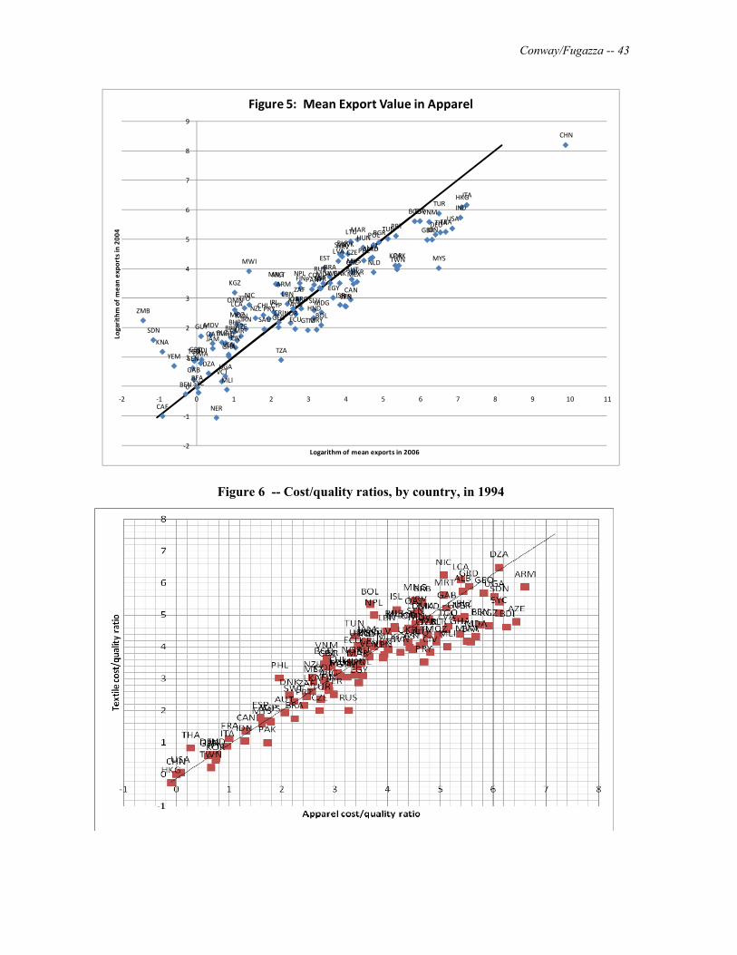
Conway/Fugazza -- 43
Figure 6 -- Cost/quality ratios, by country, in 1994
ALBARG
ARM
AUS
AUT
AZE
BDI
BENBFA
BGD
BGR
BHR
BLR
BLZ
BOL
BRA
BRB
CAF
CAN
CHL
CHN
CIVCMR
COL
CRICYP
CZE
DEU
DMA
DNK
DZA
ECU
EGY
ESP
EST
FIN
FRA
GAB
GBR
GEO
GHA
GRC
GRD
GTMGUY
HKG
HND
HRVHUN
IDN
IND
IRL
IRN
ISL
ISR
ITA
JAM
JOR JPN
KEN
KGZ
KNA
KOR
LBN
LCA
LKA
LTU
LVA
MAR
MDA
MDG
MDV
MEX
MKD
MLI
MLTMNG
MOZ
MRT
MUSMWI MYS
NER
NIC
NLD
NOR
NPL
NZLOMN
PAK
PAN
PER
PHL
POLPRT
PRY
QAT
RUS
SAU
SDN
SEN
SGP
SLV
SVKSVN
SWE
SYC
SYR
TGO
THA
TTO
TUN
TUR
TWN
TZA
UGA
UKR
URY
USA
VCT
VEN
VNM
YEM
ZAF
ZMB
‐2
‐1
0
1
2
3
4
5
6
7
8
9
‐2 ‐1 0 1 2 3 4 5 6 7 8 9 10 11
Logarithm of mean
exports in 2004
Logarithm of mean exports in 2006
Figure 5: Mean Export Value in Apparel
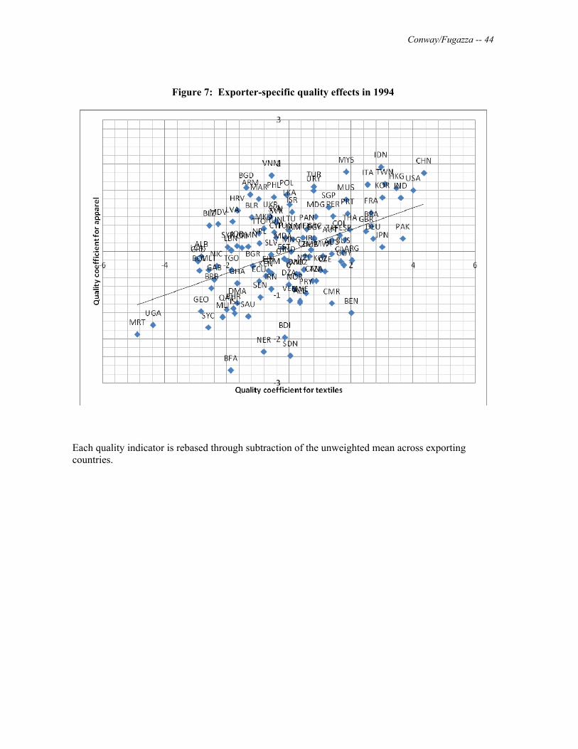
Conway/Fugazza -- 44
Figure 7: Exporter-specific quality effects in 1994
Each quality indicator is rebased through subtraction of the unweighted mean across exporting countries.
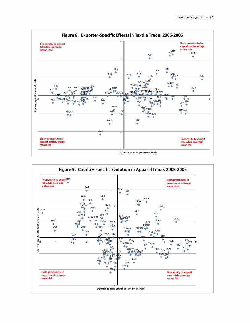
Conway/Fugazza -- 45
ALB
ARG
ARMAUS
AUT
AZE
BDI
BEN
BFA
BGD
BGR
BHR
BLR
BLZ
BOL
BRA
BRBCAN
CHLCHN
CIV
CMR
COL
CRI
CYP
CZE
DEU
DMA
DNK
DZA
ECU
EGY
ESP
ESTFIN
FRA
GAB
GBR
GEO
GHA
GRC
GRD
GTM
GUY
HKG
HND
HRV
HUN
IDNIND
IRL
IRN
ISL
ISR
ITA
JAM
JOR
JPN
KEN
KGZ
KOR
LBNLKA
LTU
LVA
MAR
MDA MDGMDV
MEX
MKD
MLI
MLT
MNG
MOZ
MRT
MUS
MWI
MYS
NER
NIC
NOR
NPL
NZLOMN
PAK
PAN
PER
PHL
POLPRTPRY
QATRUS SAU
SDN
SEN
SGP
SLV
SVK
SVNSWE
SYC
SYR
TGO
THA
TTOTUN
TUR
TWN
TZA
UGA
UKR
URYUSA
‐3
‐2
‐1
0
1
2
3
‐8 ‐6 ‐4 ‐2 0 2 4 6 8
Exporter‐specific value of trade
Exporter‐specific pattern of trade
Figure 8: Exporter‐Specific Effects in Textile Trade, 2005‐2006
Both propensity to export and average value fell
Both propensity to export and average value rose
Propensity to export fell while average value rose
Propensity to export rose while average value fell
ALB
ARG
ARM
AUS
AUT
AZEBDI
BEN
BFA
BGD
BGR
BHR
BLR
BLZ
BOL
BRA
BRBCAF
CANCHL
CHN
CIV
CMR
COL
CRI
CYP
CZE
DEU
DMA
DNK
DZA
ECU
EGY
ESP
EST
FIN
FRA
GAB
GBR
GEO
GHA
GRC
GRD
GTM
GUYHKG
HND
HRV
HUN
IDN
IND
IRL
IRNISL
ISR
ITA
JAM
JOR
JPN
KEN
KGZ
KNA
KOR
LBN
LCA
LKA
LTULVA
MAR
MDA
MDGMDV MEX
MKD
MLI
MLT
MNG
MOZ MRT
MUS
MWI
MYS
NER
NIC
NLD
NOR
NPL
NZL
OMN
PAK
PAN
PER
PHL
POL
PRT
PRY
QAT
RUS
SAU
SDN
SEN
SGP
SLV
SVKSVN
SWE
SYC
SYR
TGOTHA
TTO
TUN
TUR
TWN
TZA
UGA
UKR
URY
USA
‐1.5
‐1
‐0.5
0
0.5
1
1.5
2
‐10 ‐8 ‐6 ‐4 ‐2 0 2 4 6 8 10
Exporter‐specific effects of Value of Trade
Exporter‐specific effects of Pattern of trade
Figure 9: Country‐specific Evolution in Apparel Trade, 2005‐2006
Both propensity to export and average value rose
Both propensity to export and average value fell
Propensity to export fell while average value rose
Propensity to export rose while average value fell
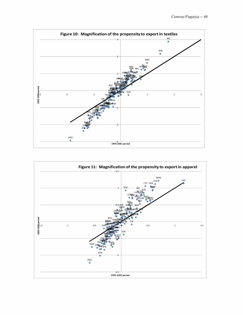
Conway/Fugazza -- 46
ALB
BGD
SAU
SDN
SEN
SGP
SLVSVK
SVN
SWE
SYCSYR
BGRTGO
THA
TTO
TUN
TUR
TWN
TZA
UGA
UKR
URY
BHR
USA
VEN
VNM
BLRBLZ
BOL
BRA
BRB
CAN
ARG
CHL
CHN
CIV
CMR
COL
CRI
CYP
CZE
DEU
DMA
ARM
DNK
DZA
ECU
EGYESP
EST
FINFRA
GAB
GBR
AUS
GEO
GHA
GRC
GRD
GTM
GUY
HKG
HND
HRV
HUN
AUTIDNIND
IRL
IRN
ISL
ISR
ITA
JAM
JOR
JPN
AZEKEN
KGZ
KOR
LBN
LCA
LKA
LTU
BDI
LVA
MARMDA
MDG
MDV
MEX
MKD
MLI
MLT
MNGBEN
MOZ
MRT
MUS
MWI
MYS
NER
NIC
NOR
NPL
NZLBFA
OMN
PAK
PANPER
PHL
POL
PRTPRY
QAT
RUS
‐3
‐2
‐1
0
1
2
3
‐3 ‐2 ‐1 0 1 2 3
2002‐2006 period
1995‐2001 period
Figure 10: Magnification of the propensity to export in textiles
ALB
BGD
SDN
SEN
SGP
SLV
SVK
SVN
SWE
SYC SYR
TGO
BGR
THA
TTO
TUN
TUR
TWN
TZA
UGA
UKR
URY
USA
BHR
BLR
BLZ
BOL
BRA
BRB
CAF
CAN
ARG
CHL
CHN
CIV
CMR
COL
CRI
CYP
CZE
DEU
DMA
ARM
DNK
DZA
ECU
EGY
ESP
EST
FIN
FRA
GAB GBR
AUS
GEO
GHA
GRCGRD
GTM
GUY
HKG
HND
HRV
HUN
AUT
IDN
INDIRL
IRN
ISL
ISRITA
JAM
JOR
JPN
AZE
KEN
KGZ
KNA
KOR
LBN
LCA
LKA
LTULVA
MARBDI
MDA
MDG
MDV MEX
MKD
MLI
MLTMNG
MOZ
MRT
BEN
MUS
MWI
MYS
NER
NIC
NLD
NOR
NPL
NZL
OMN
BFA
PAK PAN
PER
PHL
POL
PRT
PRY
QAT
RUS
SAU
‐1.5
‐1
‐0.5
0
0.5
1
1.5
‐1.5 ‐1 ‐0.5 0 0.5 1 1.5
200
2‐2006 period
1995‐2001 period
Figure 11: Magnification of the propensity to export in apparel

Conway/Fugazza -- 47
ALB
BGD
SAU
SDN
SENSGP
SLV
SVK
SVN
SWE
SYC
SYR
BGRTGO
THA
TTO
TUN
TUR
TWN
TZA
UGA
UKRURY
BHR
USA
VEN
VNM
ZAR
ZWE
BLRBLZ
BOL
BRA
BRB
CAN
ARG
CHL
CHN
CIV
CMR
COL
CRI
CYP
CZEDEU
DMA
ARM
DNK
DZA
ECU
EGY
ESP
ESTFIN
FRA
GAB
GBRAUS
GEO
GHA
GRC
GRD
GTM
GUY
HKG
HND
HRV
HUN
AUT
IDN
IND
IRL
IRN
ISL
ISR
ITA
JAM
JOR
JPN
AZE
KEN
KGZ
KOR
LBN
LCA
LKA
LTU
BDI
LVA
MAR
MDA
MDG
MDVMEX
MKD
MLI
MLT
MNG
BEN
MOZ
MRT
MUS
MWI
MYS
NER
NIC
NOR
NPL
NZL
BFA
OMN
PAKPAN
PER
PHL
POLPRT
PRYQAT
RUS
‐4
‐3
‐2
‐1
0
1
2
3
4
‐4 ‐3 ‐2 ‐1 0 1 2 3 4
2002‐2006 period
1995‐2001 period
Figure 12: The average bilateral value of trade in textiles
ALB
BGDSDN
SEN
SGP
SLV
SVK
SVN
SWE
SYC
SYR
TGO
BGR
THA
TTO
TUN
TUR
TWN
TZA
UGA
UKR
URY
USA
BHR
VCT
VEN
VNM
YEM
ZAF
ZMB
BLR
BLZ
BOL
BRA
BRB
CAF
CAN ARG
CHL
CHN
CIV
CMR
COL
CRICYP
CZE
DEU
DMA
ARM
DNK
DZA
ECU
EGY
ESP
EST
FIN
FRA
GABGBRAUS
GEO
GHA
GRC
GRD
GTM
GUY
HKG
HNDHRV
HUN
AUT
IDN
IND
IRL
IRN
ISL
ISR
ITA
JAM
JORJPN
AZE
KEN
KGZ
KNAKOR
LBN
LCA
LKA
LTU
LVAMAR
BDI
MDA
MDGMDV
MEX
MKD
MLIMLTMNG
MOZ
MRT
BEN
MUS
MWI
MYS
NER
NIC
NLD
NOR
NPLNZL
OMN
BFA
PAK PAN
PER
PHL POL
PRT
PRY
QATRUS
SAU
‐3
‐2
‐1
0
1
2
3
‐3 ‐2 ‐1 0 1 2 3
2002‐2006 period
1995‐2001 period
Table 13: Evolution of the average value of bilateral exports in apparel
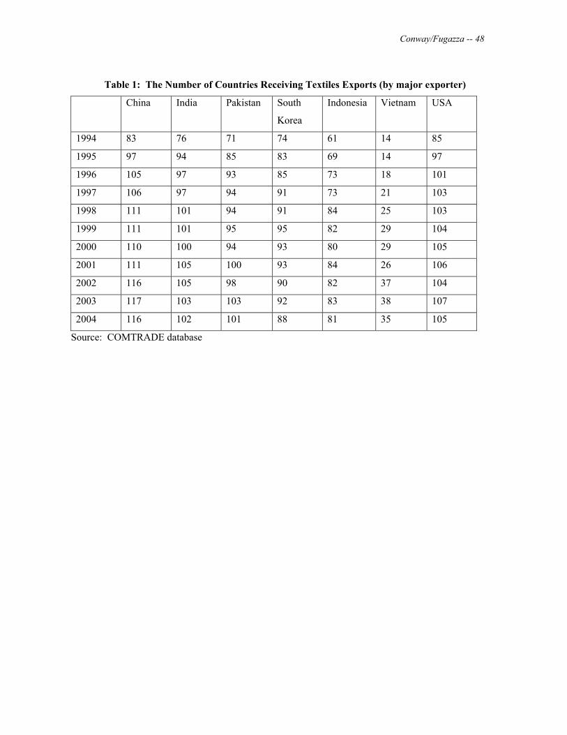
Conway/Fugazza -- 48
Table 1: The Number of Countries Receiving Textiles Exports (by major exporter)
China India Pakistan South
Korea
Indonesia Vietnam USA
1994 83 76 71 74 61 14 85
1995 97 94 85 83 69 14 97
1996 105 97 93 85 73 18 101
1997 106 97 94 91 73 21 103
1998 111 101 94 91 84 25 103
1999 111 101 95 95 82 29 104
2000 110 100 94 93 80 29 105
2001 111 105 100 93 84 26 106
2002 116 105 98 90 82 37 104
2003 117 103 103 92 83 38 107
2004 116 102 101 88 81 35 105
Source: COMTRADE database
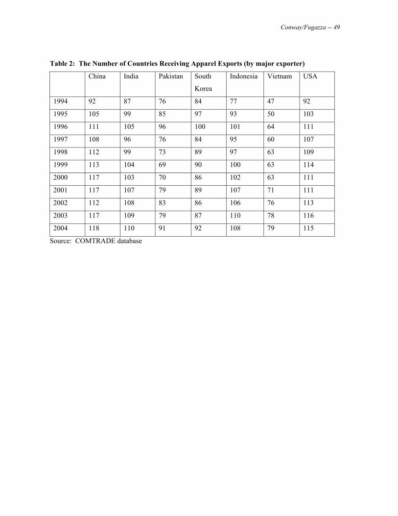
Conway/Fugazza -- 49
Table 2: The Number of Countries Receiving Apparel Exports (by major exporter)
China India Pakistan South
Korea
Indonesia Vietnam USA
1994 92 87 76 84 77 47 92
1995 105 99 85 97 93 50 103
1996 111 105 96 100 101 64 111
1997 108 96 76 84 95 60 107
1998 112 99 73 89 97 63 109
1999 113 104 69 90 100 63 114
2000 117 103 70 86 102 63 111
2001 117 107 79 89 107 71 111
2002 112 108 83 86 106 76 113
2003 117 109 79 87 110 78 116
2004 118 110 91 92 108 79 115
Source: COMTRADE database

Conway/Fugazza -- 50
Table 3: Proportion of non-zero bilateral trade pairs in sample (125 countries)
Year Textiles (652) Apparel (841/842)
1994 19.3 31.1
1995 20.1 34.5
1996 22.9 38.4
1997 22.7 30.8
1998 23.1 31.8
1999 23.7 32.1
2000 23.8 34.3
2001 24.3 35.1
2002 24.3 35.3
2003 24.6 37.1
2004 24.5 39.1
2005 25.7 41.8
2006 27.1 54.2

Conway/Fugazza -- 51
Table 4: The Quota-ridden equilibrium of 1994: estimating the pattern of trade.
Textiles Apparel
Fixed-effect probit Coefficient Standard
Error
Coefficient Standard
Error
ln(Dij) -1.07 0.04 -0.98 0.04
DBij 0.78 0.18 0.15 0.20
ln(τij94) -3.08 1.12 -1.30 2.32
N 11198 11780
Random-effect
probit
Coefficient Standard
Error
Coefficient Standard
Error
ln(Dij) -1.05 0.03 -0.97 0.03
DBij 0.72 0.14 0.14 0.16
ln(τij94) -3.47 0.98 -4.33 1.72
N 15252 15500
The fixed-effect probit includes both importer and exporter-specific indicator variables. The random-effect probit includes exporter-specific indicators and random effects clustered by importer.

Conway/Fugazza -- 52
Table 5: The quota-ridden equilibrium of 1994: estimating the value of trade.
Textiles Apparel
Non-linear
regression
Coefficient Standard
Error
Coefficient Standard
Error
ln(Yjt) 0.53 0.04 0.23 0.01
ln(Ljt) -0.03 0.05 0.06 0.02
ln(1+tijt) -0.04 0.53 0.60 6.67
ln(Dij) -0.98 0.06 -0.32 1.51
μ 5.36 0.57 1.50 1.53
φ 2.00 0.28 0.71 0.13
N 2828 4744
R2 0.70 0.87
Standard errors are robust. Each equation included exporter fixed effects used as the quality estimator.

Conway/Fugazza -- 53
Table 6: Trade in Textiles and Apparel in 2005/2006: the role of quotas
Textiles (SIC 652) Apparel (SIC 841, 842)
(22) and (23) (29) (22) and (23) (29)
ln(Dij) -0.95 -1.08 -0.83 0.35
(0.02) (0.23) (0.02) (0.29)
DBij 0.63 0.37
(0.09) (0.09)
ln(1+tijt) -2.97 -3.12 -0.71 -3.04
(0.35) (0.77) (0.27) (0.35)
ln(ĉi) -1.49 -0.94
(0.12) (0.04)
QBiUt-1 0.48 1.85
(0.18) (0.13)
QBiNt-1 -0.13 0.74 0.88 -3.32
(0.24) (0.32) (0.13) (0.44)
NBiUt-1 0.09 -0.17 0.02 0.36
(0.18) (0.09) (0.21) (0.07)
QBUjt-1 0.87 -1.14 0.29 -1.13
(0.27) (0.20) (0.28) (0.11)
T2006 0.11 -0.17 0.72 -0.52
(0.02) (0.06) (0.02) (0.24)
yjt-1 0.08 0.21
(0.01) (0.00)
ljt-1 0.56 0.08
(0.02) (0.02)
μ 0.79 2.44
(0.22) (0.34)
η 0.43 0.68
(0.12) (0.10)
Exporter-specific effects
Y Y Y Y
N 31000 7777 31000 14120
Log likelihood -7575.4 -9895.0
R2 0.51 0.80
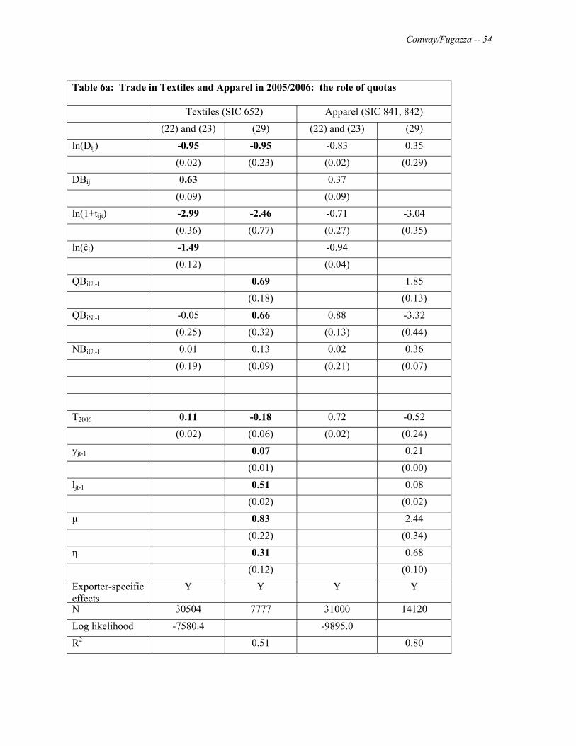
Conway/Fugazza -- 54
Table 6a: Trade in Textiles and Apparel in 2005/2006: the role of quotas
Textiles (SIC 652) Apparel (SIC 841, 842)
(22) and (23) (29) (22) and (23) (29)
ln(Dij) -0.95 -0.95 -0.83 0.35
(0.02) (0.23) (0.02) (0.29)
DBij 0.63 0.37
(0.09) (0.09)
ln(1+tijt) -2.99 -2.46 -0.71 -3.04
(0.36) (0.77) (0.27) (0.35)
ln(ĉi) -1.49 -0.94
(0.12) (0.04)
QBiUt-1 0.69 1.85
(0.18) (0.13)
QBiNt-1 -0.05 0.66 0.88 -3.32
(0.25) (0.32) (0.13) (0.44)
NBiUt-1 0.01 0.13 0.02 0.36
(0.19) (0.09) (0.21) (0.07)
T2006 0.11 -0.18 0.72 -0.52
(0.02) (0.06) (0.02) (0.24)
yjt-1 0.07 0.21
(0.01) (0.00)
ljt-1 0.51 0.08
(0.02) (0.02)
μ 0.83 2.44
(0.22) (0.34)
η 0.31 0.68
(0.12) (0.10)
Exporter-specific effects
Y Y Y Y
N 30504 7777 31000 14120
Log likelihood -7580.4 -9895.0
R2 0.51 0.80

Conway/Fugazza -- 55
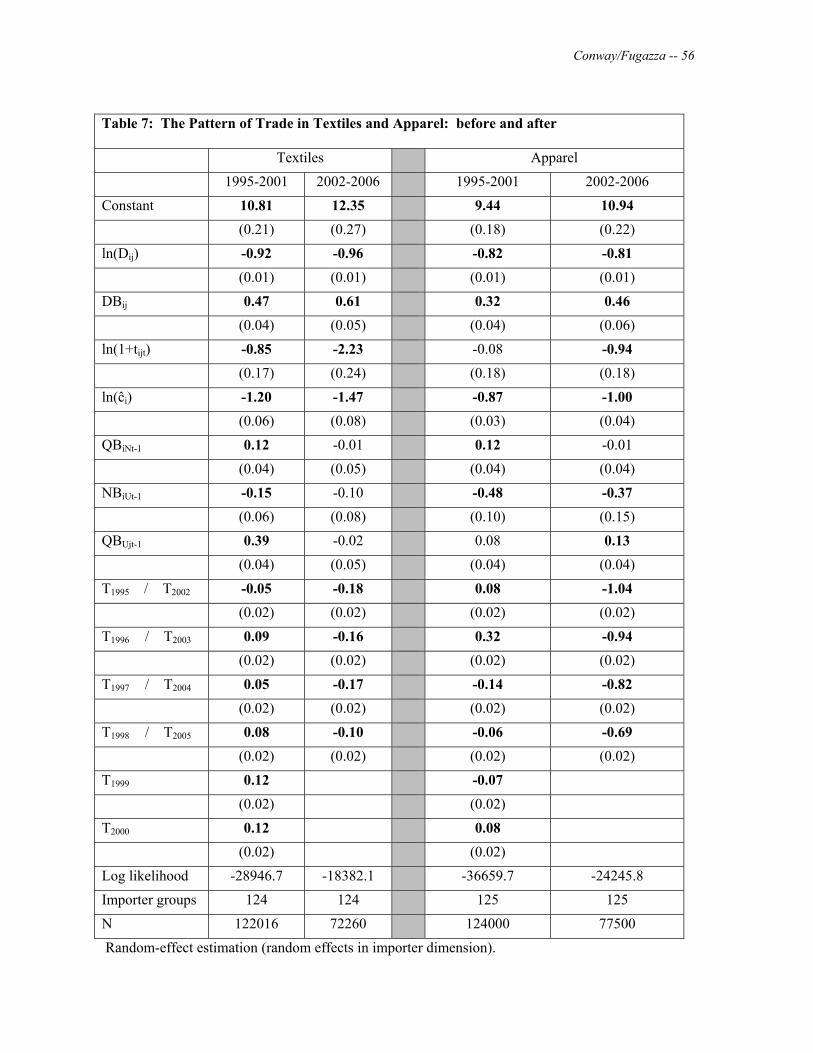
Conway/Fugazza -- 56
Table 7: The Pattern of Trade in Textiles and Apparel: before and after
Textiles Apparel
1995-2001 2002-2006 1995-2001 2002-2006
Constant 10.81 12.35 9.44 10.94
(0.21) (0.27) (0.18) (0.22)
ln(Dij) -0.92 -0.96 -0.82 -0.81
(0.01) (0.01) (0.01) (0.01)
DBij 0.47 0.61 0.32 0.46
(0.04) (0.05) (0.04) (0.06)
ln(1+tijt) -0.85 -2.23 -0.08 -0.94
(0.17) (0.24) (0.18) (0.18)
ln(ĉi) -1.20 -1.47 -0.87 -1.00
(0.06) (0.08) (0.03) (0.04)
QBiNt-1 0.12 -0.01 0.12 -0.01
(0.04) (0.05) (0.04) (0.04)
NBiUt-1 -0.15 -0.10 -0.48 -0.37
(0.06) (0.08) (0.10) (0.15)
QBUjt-1 0.39 -0.02 0.08 0.13
(0.04) (0.05) (0.04) (0.04)
T1995 / T2002 -0.05 -0.18 0.08 -1.04
(0.02) (0.02) (0.02) (0.02)
T1996 / T2003 0.09 -0.16 0.32 -0.94
(0.02) (0.02) (0.02) (0.02)
T1997 / T2004 0.05 -0.17 -0.14 -0.82
(0.02) (0.02) (0.02) (0.02)
T1998 / T2005 0.08 -0.10 -0.06 -0.69
(0.02) (0.02) (0.02) (0.02)
T1999 0.12 -0.07
(0.02) (0.02)
T2000 0.12 0.08
(0.02) (0.02)
Log likelihood -28946.7 -18382.1 -36659.7 -24245.8
Importer groups 124 124 125 125
N 122016 72260 124000 77500
Random-effect estimation (random effects in importer dimension).

Conway/Fugazza -- 57
Standard errors are reported in parentheses. Importer fixed effects are included but not reported here.
Table 8: The Value of Trade in Textiles and Apparel: before and after Textiles Apparel 1995-2001 2002-2006 1995-2001 2002-2006 ln(Yjt) 0.08 0.08 0.20 0.21 (0.003) (0.003) (0.00) (0.00) ln(Ljt) 0.36 0.47 0.06 0.04 (0.01) (0.01) (0.01) (0.01) ln(1+tijt) -3.35 -2.79 -6.01 -4.19 (0.20) (0.38) (0.16) (0.24) ln(Dij) -0.96 -1.07 0.38 -0.08 (0.13) (0.14) (0.18) (0.18) Μ 0.77 0.69 1.95 1.86 (0.13) (0.14) (0.22) (0.22) Φ 0.75 0.41 0.01 0.52
(0.07) (0.08) (0.07) (0.07)
θ̂i1.00 1.00 1.00 1.00
-- -- -- -- QBiUt-1 0.48 0.60 1.64 2.22 (0.12) (0.11) (0.17) (0.12) QBiNt-1 -0.28 0.32 -0.36 -0.21 (0.07) (0.08) (0.08) (0.07) NBiUt-1 0.10 0.01 1.92 1.41 (0.05) (0.06) (0.17) (0.16) QBUjt-1 -0.43 -0.37 -0.87 -0.59 (0.07) (0.06) (0.06) (0.05) T1995 / T2002 0.28 0.78 0.45 1.05 (0.05) (0.06) (0.04) (0.21) T1996 / T2003 0.11 0.87 -0.07 0.89 (0.05) (0.06) (0.08) (0.19) T1997 / T2004 0.09 0.68 -0.03 0.55 (0.04) (0.06) (0.05) (0.17) T1998 / T2005 0.01 0.16 -0.17 0.04 (0.04) (0.05) (0.04) (0.14) T1999 -0.12 -0.23 (0.05) (0.04) T2000 -0.26 -0.69 (0.05) (0.04) N 26504 18607 40916 31639 R2 0.47 0.50 0.84 0.80

Conway/Fugazza -- 58
Textiles: Values of Structural and Quota Variables 1995-2001 2002-2006 1995-2001 2002-2006 Pattern of trade: Value of trade: Dij 8.69 8.69 Dij 8.37 8.36 (0.002) (0.003) (0.006) (0.007) BDij 0.02 0.02 Ln(1+τijt) 0.115 0.10 (0.0004) (0.0005) (0.0006) (0.0006) Ln(1+τijt) 0.13 0.12 yjt 29.96 30.98 (0.0002) (0.0003) (0.05) (0.055) c 3.79 3.79 ljt 16.40 16.52 (0.006) (0.007) (0.01) (0.013) QBint-1 0.04 0.10 QBUjt 0.01 0.03 (0.0005) (0.001) (0.0007) (0.001) NBiUt-1 0.09 0.09 QBint-1 0.08 0.21 (0.0008) (0.001) (0.001) (0.003) QBUjt-1 0.05 0.10 NBiUt-1 0.17 0.16 (0.0006) (0.001) (0.002) (0.003) QBUjt-1 0.06 0.14 (0.002) (0.002) Rho 0.16 -7.95 (0.007) (0.009) Zee 0.87 8.08 (0.005) (0.008) N 122016 76260 26534 18632

Conway/Fugazza -- 59
Apparel: Values of Structural and Quota Variables 1995-2001 2002-2006 1995-2001 2002-2006 Pattern of trade: Value of trade: Dij 8.68 8.68 Dij 8.36 8.42 (0.002) (0.003) (0.007) (0.007) BDij 0.02 0.02 Ln(1+τijt) 0.147 0.142 (0.0004) (0.0005) (0.0006) (0.0006) Ln(1+τijt) 0.19 0.18 yjt 30.90 31.31 (0.0003) (0.0003) (0.05) (0.051) c 3.70 3.70 ljt 16.32 16.34 (0.005) (0.006) (0.012) (0.012) QBUjt-1 0.01 0.02 (0.0005) (0.001) QBiNt-1 0.03 0.12 QBiNt-1 0.05 0.16 (0.0005) (0.001) (0.001) (0.002) NBiUt-1 0.10 0.10 NBiUt-1 0.22 0.19 (0.0008) (0.001) (0.002) (0.003) QBUjt-1 0.03 0.13 QBUjt-1 0.05 0.12 (0.0005) (0.001) (0.001) (0.002) Rho 0.33 0.58 (0.008) (0.009) Zee 0.80 0.68 (0.005) (0.008) N 124000 77500 24251 21887
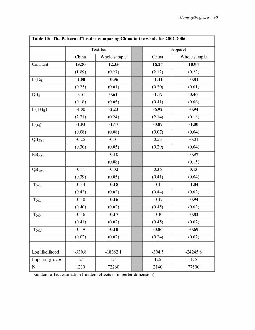
Conway/Fugazza -- 60
Table 10: The Pattern of Trade: comparing China to the whole for 2002-2006
Textiles Apparel
China Whole sample China Whole sample
Constant 13.20 12.35 18.27 10.94
(1.89) (0.27) (2.12) (0.22)
ln(Dij) -1.00 -0.96 -1.41 -0.81
(0.25) (0.01) (0.20) (0.01)
DBij 0.16 0.61 -1.17 0.46
(0.18) (0.05) (0.41) (0.06)
ln(1+tijt) -4.00 -2.23 -6.92 -0.94
(2.21) (0.24) (2.14) (0.18)
ln(ĉi) -1.03 -1.47 -0.87 -1.00
(0.08) (0.08) (0.07) (0.04)
QBiNt-1 -0.25 -0.01 0.55 -0.01
(0.30) (0.05) (0.29) (0.04)
NBiUt-1 -0.10 -0.37
(0.08) (0.15)
QBUjt-1 -0.11 -0.02 0.36 0.13
(0.39) (0.05) (0.41) (0.04)
T2002 -0.34 -0.18 -0.45 -1.04
(0.42) (0.02) (0.44) (0.02)
T2003 -0.40 -0.16 -0.47 -0.94
(0.40) (0.02) (0.45) (0.02)
T2004 -0.46 -0.17 -0.40 -0.82
(0.41) (0.02) (0.45) (0.02)
T2005 -0.19 -0.10 -0.86 -0.69
(0.02) (0.02) (0.24) (0.02)
Log likelihood -330.8 -18382.1 -304.5 -24245.8
Importer groups 124 124 125 125
N 1230 72260 2140 77500
Random-effect estimation (random effects in importer dimension).

Conway/Fugazza -- 61
Table 10: The Average Value of Trade: comparing China to the whole for 2002-2006
Textiles Apparel
China Whole sample China Whole sample
ln(yjt) 0.09 0.08 0.25 0.21
(0.02) (0.003) (0.01) (0.00)
ln(ljt) 0.48 0.47 0.08 0.04
(0.05) (0.01) (0.05) (0.01)
ln(Dij) -0.54 -1.07 0.92 -0.08
(0.06) (0.14) (0.34) (0.18)
ln(1+tijt) 1.76 -2.79 -1.46 -4.19
(1.13) (0.38) (2.10) (0.24)
Mu 1.09 0.69 0.87 1.86
(0.08) (0.14) (0.27) (0.22)
zee 0.32 0.41 -1.54 0.52
(0.29) (0.08) (1.11) (0.07)
QBiUt-1 -0.48 0.60 0.16 2.22
(0.48) (0.11) (0.34) (0.12)
QBiNt-1 -0.45 -0.37 -1.05 -0.21
(0.27) (0.06) (0.32) (0.07)
NBiUt-1 0.01 1.41
(0.06) (0.16)
QBUjt-1 -0.26 -0.37 -0.39 -0.59
(0.27) (0.06) (0.22) (0.05)
T2002 -0.78 0.78 -2.11 1.05
(0.34) (0.06) (0.36) (0.21)
T2003 -0.55 0.87 -2.03 0.89
(0.34) (0.06) (0.36) (0.19)
T2004 -0.35 0.68 -2.06 0.55
(0.34) (0.06) (0.34) (0.17)
T2005 0.11 0.16 -0.91 0.04
(0.22) (0.05) (0.30) (0.14)
N 864 18607 843 31639
R2 0.59 0.50 0.86 0.80
Random-effect estimation (random effects in importer dimension).

Conway/Fugazza -- 62

Conway/Fugazza -- 63
Table 9: The Value of Trade in Apparel with linkages 2005/2006 Early period Later years
Pattern of trade Value of trade Pattern of trade Value of trade Pattern of trade Value of trade
ŝijt 0.28 1.36 0.08
(0.12) (0.32) (0.12)
ŝjit 0.42 3.47 0.40
(0.05) (0.48) (0.05)
QBiUt-1 1.12
(0.13)
QBiNt-1 0.01
(0.04)
NBiUt-1 0.23 1.52 -0.33
(0.23) (0.27) (0.14)
QBUjt-1 0.43 -3.80 0.12
(0.22) (0.49) (0.04)
T2006 0.64 5.43
(0.02) (0.74)
N 30504 14225 76260
R2 0.87 0.84 0.83 0.62
Standard errors are reported in parentheses.

Conway/Fugazza -- 64
Table 11: How well do we predict (in-sample) the pattern of trade in textiles? Column 2:
Predicted trade? Column 3: Predicted trade?
Column 4: Predicted trade?
Actually trading?
Yes No Yes No Yes No Yes No
Yes 129788 1325 128828 2285 128369 2744 124680 6433 No 32192 7195 28738 10649 27426 11961 20257 19130
Correctly classified (percent)
80.3 81.8 82.3 84.3
The predicted trade is derived in each case by setting the cut-off probability at 0.5.
Table 12: How well do we predict (in sample) the pattern of trade in apparel?
Column 2: Predicted trade? Column 2: Predicted trade?
Column 3: Predicted trade? Column 4: Predicted trade?
Actually trading?
Yes No Yes No Yes No Yes No
Yes 108114 3577 107920 3771 107740 3951 107876 3815 No 40441 18363 38203 20606 37522 21287 37831 20978 Correctly classified (percent)
74.2 75.4 75.7 75.6
The predicted trade is derived in each case by setting the cut-off probability to 0.50.
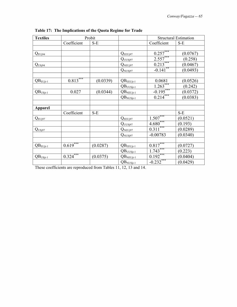
Conway/Fugazza -- 65
Table 17: The Implications of the Quota Regime for Trade
Textiles Probit Structural Estimation Coefficient S-E Coefficient S-E QEUj94
QEEUj97 0.257*** (0.0767) QUUSj97 2.557*** (0.258) QUSj94 QNEUj97 0.213*** (0.0467) QNUSj97 -0.141** (0.0493) QBEUjt-1 0.813*** (0.0339) QBEEUjt-1 0.0681 (0.0526) QBUUSjt-1 1.263*** (0.242) QBUSjt-1 0.027 (0.0344) QBNEUjt-1 -0.195*** (0.0372) QBNUSjt-1 0.214*** (0.0383) Apparel Coefficient S-E S-E QEUj97
QEEUj97 1.507*** (0.0521) QUUSj97 4.680*** (0.193) QUSj97
QNEUj97 0.311*** (0.0289) QNUSj97 -0.00783 (0.0340) QBEUjt-1 0.619*** (0.0287) QBEEUjt-1 0.817*** (0.0727) QBUUSjt-1 1.743*** (0.223) QBUSjt-1 0.324*** (0.0375) QBNEUjt-1 0.192*** (0.0404) QBNUSjt-1 -0.232*** (0.0429) These coefficients are reproduced from Tables 11, 12, 13 and 14.
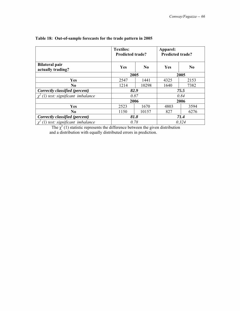
Conway/Fugazza -- 66
Table 18: Out-of-sample forecasts for the trade pattern in 2005
The χ2 (1) statistic represents the difference between the given distribution and a distribution with equally distributed errors in prediction.
Textiles: Predicted trade?
Apparel: Predicted trade?
Bilateral pair actually trading? Yes No Yes No
2005 2005 Yes 2547 1441 4325 2153 No 1214 10298 1640 7382
Correctly classified (percent) 82.9 75.5 χ2 (1) test: significant imbalance 0.87 0.84
2006 2006 Yes 2523 1670 4803 3594 No 1150 10157 827 6276
Correctly classified (percent) 81.8 71.4 χ2 (1) test: significant imbalance 0.78 0.324
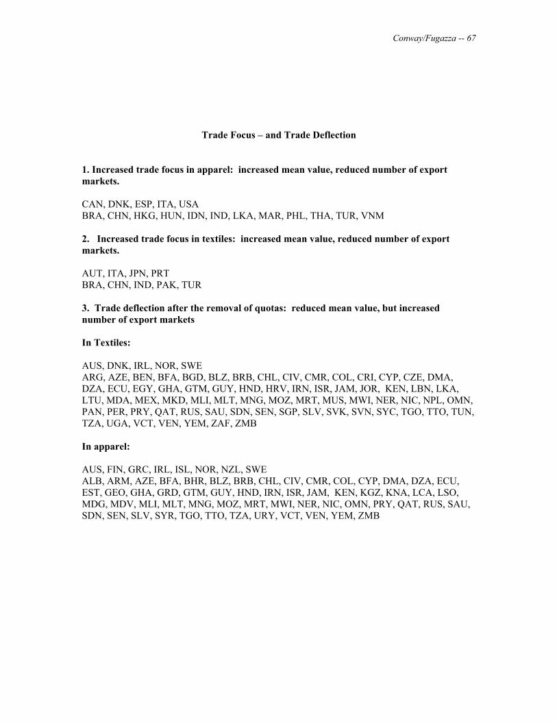
Conway/Fugazza -- 67
Trade Focus – and Trade Deflection
1. Increased trade focus in apparel: increased mean value, reduced number of export markets. CAN, DNK, ESP, ITA, USA BRA, CHN, HKG, HUN, IDN, IND, LKA, MAR, PHL, THA, TUR, VNM 2. Increased trade focus in textiles: increased mean value, reduced number of export markets. AUT, ITA, JPN, PRT BRA, CHN, IND, PAK, TUR 3. Trade deflection after the removal of quotas: reduced mean value, but increased number of export markets In Textiles: AUS, DNK, IRL, NOR, SWE ARG, AZE, BEN, BFA, BGD, BLZ, BRB, CHL, CIV, CMR, COL, CRI, CYP, CZE, DMA, DZA, ECU, EGY, GHA, GTM, GUY, HND, HRV, IRN, ISR, JAM, JOR, KEN, LBN, LKA, LTU, MDA, MEX, MKD, MLI, MLT, MNG, MOZ, MRT, MUS, MWI, NER, NIC, NPL, OMN, PAN, PER, PRY, QAT, RUS, SAU, SDN, SEN, SGP, SLV, SVK, SVN, SYC, TGO, TTO, TUN, TZA, UGA, VCT, VEN, YEM, ZAF, ZMB In apparel: AUS, FIN, GRC, IRL, ISL, NOR, NZL, SWE ALB, ARM, AZE, BFA, BHR, BLZ, BRB, CHL, CIV, CMR, COL, CYP, DMA, DZA, ECU, EST, GEO, GHA, GRD, GTM, GUY, HND, IRN, ISR, JAM, KEN, KGZ, KNA, LCA, LSO, MDG, MDV, MLI, MLT, MNG, MOZ, MRT, MWI, NER, NIC, OMN, PRY, QAT, RUS, SAU, SDN, SEN, SLV, SYR, TGO, TTO, TZA, URY, VCT, VEN, YEM, ZMB

Conway/Fugazza -- 68
Appendix : Characteristics of restraints on textiles and apparel imports to the US and EU.
The system of bilateral quantitative restraints (or quotas) on textile and apparel imports
was an enduring feature of the US and European Union (EU) commercial policy system. From its
inception in the early 1960s with the Long-Term Arrangement in Cotton Textiles (LTA), through
its codification in the Multi-Fiber Arrangement (MFA) from 1974 to 1995, and to its 1995-2005
form in the Agreement on Textiles and Clothing (ATC), the system provided protection to US
and EU producers of textiles and apparel.34
In the negotiations that led to the adoption of the ATC in 1995, the US and EU agreed to
dismantle the system of quantitative restraints sequentially. A large number of restraints was
removed at the beginning of 1995, 1998 and 2002, but those remaining governed trade in the
categories of textiles and apparel most produced in the US and EU. These remaining restraints
were removed on 1 January 2005. The ATC by its end had evolved into a complicated
interlocking set of bilateral agreements on quantities exported. They acted as export restraints,
but they were binding in any given year on only a small subset of the countries under restraint.
Specific limits and group limits interacted in non-transparent ways to limit a given country’s
exports.
The basic unit of the quota system was the restraint category, or quota category. These
categories were defined as aggregated subgroups of textile and apparel products with some shared
characteristic or raw material. The system of import restraints defined by the US identified 11
aggregated categories of yarns, 34 aggregated categories of textiles, 86 categories of apparel and
16 categories of miscellaneous textiles (e.g., towels). Together these categories spanned the
entire set of US textile and apparel imports. The EU identified 41 categories of yarns, 28
categories of textiles, 42 categories of apparel and 32 categories of miscellaneous textiles for a
total of 143 categories – although some of these categories were further subdivided by raw
material.35 Each category included multiple products. For example, US category 225 (blue
denim) was aggregated from 16 distinct HS product lines. Products included in each category
were similar, but could have significant differences: for example, the “blue denim” category
included denim made from both cotton and man-made fibers. There is no corresponding category
34 Francois et al. (2007) provides a detailed discussion of this chronology. There were actually six groupings that imposed bilateral quotas under the MFA and ATC: in addition to the EU and US, there were Canada, Norway, Finland and Austria. The work in this paper focuses upon the US and EU, but the analysis will be extended to the others in future research. 35 The categories for the US, and the correspondence between those categories and the HS classification of imports, are published by the Office of Textiles and Apparel (OTEXA), Department of Commerce, at http://otexa.ita.doc.gov/corr.htm. The categories for the EU, and concordance with CN category, are published in EEC Council Regulation 3030/93 of 12 October 1993.
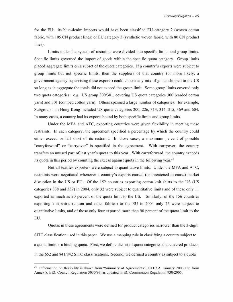
Conway/Fugazza -- 69
for the EU: its blue-denim imports would have been classified EU category 2 (woven cotton
fabric, with 105 CN product lines) or EU category 3 (synthetic woven fabric, with 80 CN product
lines).
Limits under the system of restraints were divided into specific limits and group limits.
Specific limits governed the import of goods within the specific quota category. Group limits
placed aggregate limits on a subset of the quota categories. If a country’s exports were subject to
group limits but not specific limits, then the suppliers of that country (or more likely, a
government agency supervising these exports) could choose any mix of goods shipped to the US
so long as in aggregate the totals did not exceed the group limit. Some group limits covered only
two quota categories: e.g., US group 300/301, covering US quota categories 300 (carded cotton
yarn) and 301 (combed cotton yarn). Others spanned a large number of categories: for example,
Subgroup 1 in Hong Kong included US quota categories 200, 226, 313, 314, 315, 369 and 604.
In many cases, a country had its exports bound by both specific limits and group limits.
Under the MFA and ATC, exporting countries were given flexibility in meeting these
restraints. In each category, the agreement specified a percentage by which the country could
either exceed or fall short of its restraint. In those cases, a maximum percent of possible
“carryforward” or “carryover” is specified in the agreement. With carryover, the country
transfers an unused part of last year’s quota to this year. With carryforward, the country exceeds
its quota in this period by counting the excess against quota in the following year.36
Not all textiles exporters were subject to quantitative limits. Under the MFA and ATC,
restraints were negotiated whenever a country’s exports caused (or threatened to cause) market
disruption in the US or EU. Of the 152 countries exporting cotton knit shirts to the US (US
categories 338 and 339) in 2004, only 32 were subject to quantitative limits and of these only 11
exported as much as 90 percent of the quota limit to the US. Similarly, of the 156 countries
exporting knit shirts (cotton and other fabrics) to the EU in 2004 only 25 were subject to
quantitative limits, and of those only four exported more than 90 percent of the quota limit to the
EU.
Quotas in these agreements were defined for product categories narrower than the 3-digit
SITC classification used in this paper. We use a mapping rule in classifying a country subject to
a quota limit or a binding quota. First, we define the set of quota categories that covered products
in the 652 and 841/842 SITC classifications. Second, we defined a country as subject to a quota
36 Information on flexibility is drawn from “Summary of Agreements”, OTEXA, January 2003 and from Annex 8, EEC Council Regulation 3030/93, as updated in EC Commission Regulation 930/2005.

Conway/Fugazza -- 70
limit if the US or EU had specified a quota limit for that exporting country in any one of those
categories. Third, following Dean (1990) and Dean (1995), we categorized an exporting country
as subject to a binding quota if its observed quantity exported in that year was greater than 90
percent of the quota limit. We used data provided by the OTEXA Division of the US Department
of Commerce and by the EU to calculate this percentage.
Table A1 -- Quota limits (and binding quotas) in 1994
US – textiles (25/13)
EU – textiles (41/11)
US – apparel (44/34)
EU – apparel (46/16)
ARE, BRA, CHN*, ALB, ARE, ARG, ARE*, BGD*, BHR, ALB, ARE, ARM,
COL, CZE, EGY*, ARM, AZE, BGR*, BRA, CHN*, COL*, AZE, BGD, BGR,
HKG*, HUN, IDN*, BLR, BRA, CHN*, CRI*, CZE, DOM*, BLR*, BRA, CHN*,
IND*, LKA, KOR*, CZE*, EGY, EST, EGY*, FJI*, GTM*, CZE, EGY, EST,
MAC, MUS, MYS*, GEO, HKG, HUN, HKG*, HND, HUN, GEO, HKG*, HUN,
PAK*, PHL*, POL, IDN*, IND*, IDN*, IND*, JAM*, IDN*, IND*,
ROM*, SGP, SVK, KGZ, KOR*, KSV, KEN, KOR*, KWT, KGZ, KOR*, KSV,
THA*, TUR*, TWN*, LTU, LVA, MDA, LAO*, LKA*, MAC*, LKA*, LTU, LVA,
URY MKD, MLT, MYS, MKD*, MMR, MUS*, MAC*, MAR, MDA,
PAK*, PER, POL*, MYS*, NPL*, OMN*, MKD, MLT, MNG,
ROM, SGP, SVK, PAK*, PHL*, POL*, MYS*, PAK*, PHL*,
SVN, THA*, TJK QAT*, ROM*, RUS*, POL, ROM*, SGP,
TKM, TUN, TWN*, SGP*, SLV*, SVK, SVK, SVN, THA*,
UZB, VNM* THA*, TUR*, TWN*, TJK, TKM, TUN,
UKR*, URY TWN*, UKR*, UZB,
VNM*
Sources: authors’ calculations
Table A1 indicates the countries subject to quota limits in 1994 – these were the countries i
designated with 1 in QEUi94 and QUSi94. Those with binding quotas in 1994 are marked with an
asterisk. The totals of countries with quota limits and with binding quotas are given in
parentheses at the top of each column. Note that the number of countries with quota limits is
relatively small compared to the total universe of potential exporters. Note also that the
percentage of countries with binding quotas is relatively high due to the aggregation performed
here. In any single quota category, the number of countries subject to binding quotas will
typically be closer to 10 percent. See Conway (2007) for examples.
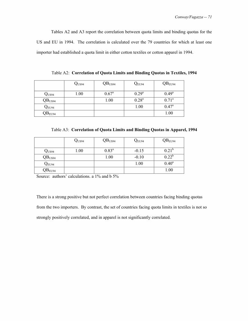
Conway/Fugazza -- 71
Tables A2 and A3 report the correlation between quota limits and binding quotas for the
US and EU in 1994. The correlation is calculated over the 79 countries for which at least one
importer had established a quota limit in either cotton textiles or cotton apparel in 1994.
Table A2: Correlation of Quota Limits and Binding Quotas in Textiles, 1994
QUS94 QBUS94 QEU94 QBEU94
QUS94 1.00 0.67a 0.29a 0.49a
QBUS94 1.00 0.28a 0.71a
QEU94 1.00 0.47a
QBEU94 1.00
Table A3: Correlation of Quota Limits and Binding Quotas in Apparel, 1994
QUS94 QBUS94 QEU94 QBEU94
QUS94 1.00 0.83a -0.15 0.21b
QBUS94 1.00 -0.10 0.22b
QEU94 1.00 0.40a
QBEU94 1.00
Source: authors’ calculations. a 1% and b 5%
There is a strong positive but not perfect correlation between countries facing binding quotas
from the two importers. By contrast, the set of countries facing quota limits in textiles is not so
strongly positively correlated, and in apparel is not significantly correlated.