1

Taking Advantage of Global Diversification:

A Mutivariate-Garch Approach

Elena Kalotychou*, Sotiris K. Staikouras, Gang Zhao

Cass Business School, City University London, 106 Bunhill Row, London EC1Y 8TZ

First draft: June 2008. This version: May 2009.

Abstract

We gauge the economic value of multivariate covariance estimators by assessing the

risk-return performance of the resulting mean-variance efficient portfolios. A dynamic asset

allocation framework is deployed, where the multivariate covariance forecasts compete

against simpler nonparametric rivals widely used in the industry. A two-layer portfolio

construction process for global asset allocation is developed to overcome the problem of

handling large dimensional covariance structures. Based on an out-of-sample volatility

timing setup the empirical results suggest that the multivariate covariance forecasts

outperform their nonparametric counterparts and the proposed two-layer global asset

allocation is favored over conventional portfolio selection approaches.

JEL Classification: C32, C52, C53, F21, G11, G15

Keywords: Dynamic Conditional Correlation, Asymmetry, Covariance forecast, Dynamic

Asset Allocation, Portfolio performance.

The authors would like to thank participants at the 28th International Symposium on Forecasting, June 2008, Nice, the British Accounting Association Annual Conference, April 2009, Dundee, the FMA European Meeting, June 2009, Turin, the Multinational Finance Society Conference, July 2009, Crete, and seminar participants at Cass Business School for useful comments. The usual disclaimer applies. *Corresponding author: Tel. +44(0) 207 040 5259; E-mail: e.kalotychou@city.ac.uk (E. Kalotychou)

2

2.1 INTRODUCTION

There has been a voluminous literature on time series models for the estimation of asset

covariances, and many different specifications have been proposed for this purpose. Most

previous studies either focus on the theoretical properties of novel estimators or compare

them from a statistical point of view. As inferences in regards to the relative performance of

alternative covariance estimators have been largely confined to the use of statistical

evaluation metrics, the debate regarding the economic gains of different covariance models

is still open-ended.

The practical usefulness of multivariate time-varying covariance estimators to asset

allocation has been hindered by the lack of an appropriate way to handle a large number of

assets. Estimating variance-covariance matrices using the entire asset set typically entails

huge computational burden of maximizing the likelihood, whereas two-step quasi

likelihood approaches become biased due to the incidental parameters problem. The

question of fitting large dimensional time-varying covariance models has also caused an

upsurge of recent research (Engle, Shephard and Sheppard, 2008).

In this study, we confront alternative multivariate covariance estimators from a tactical

asset allocation perspective. The contribution to the extant literature is threefold. First,

the covariance estimators are assessed on the basis of on economic value — relative forecast

accuracy is gauged by the ability to yield superior risk-return portfolio performance.

Second, while previous studies mainly focused on in-sample comparisons an out-of-sample

evaluation is conducted, where two forecasting settings for the multivariate covariance

models are deployed. In addition, the RiskMetrics exponential smoother that has been

widely used in the industry as a simple and viable way of estimating conditional

covariances when faced with a large number of assets is used as a rival to assess the

potential gains from multivariate covariance models. Historical moving average and

random walk forecasts are also used as ‘naïve’ benchmarks. Third, we propose a novel

way to tackle the problem encountered in the estimation of time-varying covariances for

high dimensional portfolios of hundreds of assets. We sidestep estimating the covariance

matrix for a huge asset set, by dividing the estimation process in two-layers, namely, the

national market and the domestic market layer. The approach is demonstrated in the

context of global sector allocation.

The empirical evidence suggests that there is substantial economic value in

time-varying multivariate covariance forecasts. Incorporating multivariate conditional

covariance models in the asset allocation strategy generates a better risk-return profile than

3

the portfolio based on the simple covariance forecasts. Furthermore, the proposed

two-layer global asset allocation strategy outperforms the conventional approach by

providing investment superior performance irrespective of the portfolio construction

technique employed.

The remainder of the paper is organized as follows. Section 2.2 reviews the related

literature. Section 2.3 describes the data used and provides some summary statistics.

Section 2.4 delineates the time-varying covariance models and develops the forecasting

framework and the novel global asset allocation strategy. Section 2.5 reports the empirical

results and Section 2.6 concludes.

2.2 BACKGROUND LITERATURE

A burgeoning area in financial economics has been the volatility dynamics of asset returns

and their comovement. The integration of modern financial markets and the booming of

structured financial instruments (such as derivatives) have both contributed to this research

trend. In what follows, this section explores the literature related to the covariance

dynamics of financial assets and their impact on global diversification.

2.2.1 Stylized facts of Volatility and Correlation

There is an extensive literature on the relationship between stock returns and their volatility,

and the consensus is that volatility is time-varying and asymmetric in nature. Black (1976)

conducted the first empirical study on the relation between stock returns and volatility. He

found that volatility was typically higher after the stock market falls than after it rises, so

future conditional stock volatility was negatively linked with the current stock return.

Black argued that the phenomenon may be due to the increase in leverage surfacing when

the market value of a firm declines. In a similar fashion, Christie (1982) documented

parallel results on a larger sample size (379 firms) over a longer sample period (1962-78).

The above findings are further supported by Schwert (1989), who analyzed the relation of

stock volatility a economic activity, financial leverage and stock trading activity using

monthly market indices from 1857 to 1987.

The “leverage” and “volatility feedback” interpretations of asymmetric volatility differ in

regards of causalities: leverage hypothesis rests on the conjecture that return shocks lead to

changes in conditional volatility; whereas the volatility feedback theory contends that return

shocks are caused by changes in conditional volatility. Bekaert & Wu (2000) provided a

new framework to examine the two potential explanations of the asymmetry, which is a

4

Conditional Capital Asset Pricing Model (CAPM) model with a GARCH-M

parameterization. They observed the peaks in the portfolio volatility typically correspond

to large market declines and suggested that “volatility feedback” was the dominant cause of

volatility asymmetry. In addition, they showed the main mechanism behind asymmetry

for high and medium leverage portfolios was covariance asymmetry i.e. negative shocks

substantially increase betas (conditional covariances between portfolio returns and market

portfolio), while positive shocks had a mixed impact on betas.

There is also evidence suggesting that price fluctuations in one asset can transmit to other

assets. This phenomenon is usually known as volatility spillovers, and has attracted the

attention of academics and practitioners alike. At an international level, the consensus

view is that the linkage among global markets has been strengthened by the integration of

financial markets and the growing trading activity among countries. The silent culprits

behind such a trend have been the free flow of goods and capital, as well as the revolution in

information technology.

Eun & Shim (1989) investigated the international transmission mechanism of stock

market movements, and documented substantial amount of interdependence in

international equity markets. The observed innovations occurring in the US market

(1979-1985) rapidly transmitted to other markets simultaneity and in the same direction. In

contrast, the information transmissions from small markets to big markets were found to be

weak and not significant, while the reverse route was far more pronounced. Koutmos &

Booth (1995) investigated the transmission mechanism of price returns and volatility across

the US, UK and Japanese markets. They found strong evidence that volatility spillovers in

a given market were much more pronounced when the news arriving from the last market

was bad, i.e. negative shocks increase volatility transmission considerably more than

positive shocks. Baele (2003) examined the magnitude and time-varying nature of

volatility spillovers from the aggregate indices of European (EU) and US markets to 13 local

European equity market indices and documented an asymmetric effect. The US, as a proxy

for the world market, continued to be the dominate influence in European equity markets.

Contagion increases during periods high equity market volatility. Worthington & Higgs

(2004) analyzed the transmission of equity returns and volatility between developed and

Asian equity markets. The evidence suggested that all Asian markets are highly integrated,

and their co-movement escalated significantly when domestic volatility increased.

The price and volatility spillover phenomenon is also well documented at a company

level within national equity markets. Conrad, Gultekin & Kaul (1991) showed that in the

5

US equity market (all firms recorded on the CRSP tape) there was a size asymmetry in the

predictability of the volatilities transmission of large versus small firms over 1962-1988.

Harris & Pisedtasalasai (2006) investigated the return and volatility transmission

mechanisms between large and small stock in the US stock and showed that returns and

volatilities of large stocks were important in predicting the future dynamics of smaller

stocks, but not vice versa.

More recently, the research focus has recently shifted towards modeling the

dynamics of correlations and covariance. Understanding the dynamics of conditional

covariance is crucial for international portfolio diversification. Bollerslev, Engle &

Wooldridge (1988) showed that the conditional covariances between financial assets were

time-varying. Longin & Solnik (1995) argued that correlations between international equity

markets increased over time. Similarly, Ang & Bekaert (1999) found, via a regime

switching framework, evidence for the existence of a high volatility regime, in which

monthly returns (MSCI for US, UK and Germany 1970-97) were more correlated and had

lower means. In line with the previous empirical evidence (Longin & Solnik, 1995) on

integrated equity markets, they also documented the presence of a high volatility-high

correlation regime which tended to coincide with a bear market.

At the same time, it is true those financial markets are procyclical, and that business

cycles affect the intensity of price movements and the associated correlations. Along these

lines, Erb, Harvey & Viskanta (1994) linked the time variation in correlations to the phases of

business cycles. They investigated the economic changes of the G-7 industrial countries

and found that correlations are higher in recessions relative to expansions, and low when

two countries’ business cycles are out of phase. Longin & Solnik (2001) investigate the

time-varying nature of correlation between financial assets by deploying extreme value theory

to the conditional correlation of extreme observations. Using monthly equity index returns

for the five largest equity markets across the world from 1959 to 1996 they corroborate

previous findings, that correlations rise in bear markets, but not in bull markets.

Bekaert, Harvey & Ng (2005) attempted to explain the cause of asymmetric

correlation at market level, especially in extreme cases i.e. during financial crises. They

proposed an asset pricing model, which posited that changes in conditional correlation were

caused by global, regional and country-specific fundamentals and found that for some crises

(e.g. Mexican crisis, 1994), the sudden jump in cross-correlation between indices was a result

of both market’s excess returns being exposed to a common factor and not of volatility

spillovers. However, they did find economically meaningful increases in the residual

6

correlation1 in Asia, during the crisis.

Although most of the empirical studies in this area have accepted the fact that

correlation and covariance do vary over time, it is only until recently, that researchers have

started to observe and analyze the structural breaks in the time-varying correlations. Billio

& Pelizzon (2003) documented an increase in the conditional correlation of European equity

markets in the aftermath of the EMU introduction, and that the effect was not only regional,

but also had a fundamental impact on global markets. Cappiello, Engle & Sheppard (2006)

proposed an Asymmetric Generalized DCC multivariate model (AG-DCC) to capture

correlation dynamics. They examined daily data on FTSE All-World stock market indices

of 21 countries, and the 5-year average maturity bond indices for the 13 countries over

1987-01. They found strong evidence of asymmetries in conditional covariance of both

equity and bond returns. More importantly, they documented significant evidence of a

structural break. That is, when the EMU was introduced in January 1999, the level of

conditional correlation significantly increased, but this sort of increase had not been found

in the level of conditional volatility. Hyde, Bredin & Nguyen (2007) investigated the

weekly correlation dynamics across 13 Asia-Pacific equity markets, a European index and

the US market index 2 over 1991-06. Similar to previous studies, they established

significant asymmetries in correlations, a structural break for the Asian crisis and an increase

in correlations over time reinforcing the greater market integration.

2.2.5 International Diversification

Diversification is the answer to the enhancement of the risk-return profile in any investment

decision, and the fund management profession has relied on this principle for a number of

decades to manage a vast amount of wealth. The increased trend of financial globalization

and market integration, however, has prompted the question of whether international

diversification is still an effective risk reduction approach. The question becomes even

more relevant when financial crises and their associated effects come under the spotlight.

A few decades later, Markowitz (1952) produced one of the most valuable

breakthroughs in the modern investment management arena. He formalized the intuition

of portfolio theory and proposed a portfolio selection technique on the basis of its risk-return

profile, as opposed to merely compiling portfolios with assets that individually have

1 The residual correlation refers to the correlation of the exceed returns, or, the residual errors from the corresponding return equations. 2 The 13 Asia-Pacific equity markets are presented by their domestic stock exchange indices. The index for US market is S&P500 and the index for European market is a value weighted index of returns from France, Germany, Italy and the UK.

7

attractive characteristics. Tobin (1958) expanded Markowitz’s (1952) work by adding a

risk-free asset to the analysis. This made it possible to leverage or deleverage portfolios on

the efficient frontier. Through leverage, portfolios on the capital market line were able to

outperform portfolios on the efficient frontier.

Solnik (1976) produced the first formal study on international diversification. Using

weekly US and European data, over 1966-71, he showed that through international

diversification, investors can get a portfolio with much lower aggregate volatility compare

to domestic diversification. His findings indicated that in domestic markets, the number of

securities within a portfolio was negatively related to portfolio risk (in line with Markowitz,

1952), while even greater reduction of risk can be attained by diversifying internationally.

De Santis & Gerard (1997) argued that although severe market declines were contagious,

gains from international diversification were still achievable. Using monthly MSCI

dollar-denominated returns on stock indices for the G7 plus Switzerland3 and a conditional

CAPM model with multivariate GARCH-M they showed that spillover effects on price and

volatility are short-lived (several days in most cases), and will not have significant impacts

on a portfolio diversified globally, rebalanced on a low frequency (e.g. monthly or quarterly).

The findings suggested that although holding an internationally diversified portfolio

provided little protection against severe US market declines, the long-term benefits from the

diversification still remained economically attractive.

Recently, Ang & Bekaert (1999, 2002) showed that, a high volatility-high correlation

regime did exist, which tended to coincide with a bear market. However, by examining the

relationship between the US, UK and German markets from 1970s to 1990s, they found the

evidence on higher volatility was much stronger than the evidence on higher correlation and

lower means. They suggested that the benefits of international diversification still existed

even in the high correlation regime for long investment horizons.

Goetzmann, Li & Rouwenhorst (2005) used a long span of historical data to

investigate whether global diversification strategies served investors well over the last

century, and the potential of international diversification in the future. In order to explain

the benefits from global diversification, they decomposed them into a) the variation in the

average correlation in equity markets through time and b) the variation in the investment

opportunity set. From 1850 till 2000, all the available data on over 80 international equity

markets had been collected. The analysis suggested that the structure of global correlations

shifted considerably over time, and it was currently near its historical high. They found

3 The largest European market not included in the G7.

8

that approximately fifty percent of the diversification benefits that achieved by investors

today were due to the increasing number of new investment opportunities in the world

markets; and the other half due to a lower average correlation between the recently available

markets and existing markets, and among the new markets themselves.

2.2.6 Evaluation of Covariance Estimators

The upshot of the extant literature is that although, under extreme conditions,

investors cannot gain extra protection from global diversification, the long-term benefits are

still attainable. Since global asset allocation is still an attractive investment route, the

efficient construction of such a global portfolio comes to the forefront. The key input is the

asset covariance structure but the question emanating is whether it pays off to try and

accurately capture all the stylized facts of covariance structure of asset returns.

De Santis & Gerard (1997) noted that the co-movements between financial assets

were short-lived, which negates the value of accounting for correlation dynamics in a

long-term investment strategy. Fleming, Kirby & Ostdiek (2001) examined the economic

value of volatility timing for short-horizon investors in equity, bond and gold futures.

They found that the predictability captured by conditional volatility models is economically

significant and the dynamically formed portfolio outperforms the unconditionally efficient

static portfolio with the same target expected return and transaction costs.

Balasubramanyan (2004) compared the performance of portfolios constructed on the

basis of different variance-covariance matrix estimation approaches. Portfolios consisting

of US, UK and Japan stocks were rebalanced daily and six multivariate GARCH models had

been employed. The portfolio incorporating time-varying correlation with asymmetric

volatility and spillovers outperformed its simple counterpart that ignored such information.

Engle & Colacito (2006) investigated the variance minimization problem subject to a

required return. They derived an important result, that the efficiency loss of the portfolio

was minimized when the estimated correlation was equal to the “true” value. Using a

two-asset framework, they calculated the loss of efficiency4 while keeping the assets’

expected returns fixed. They demonstrated that the asymmetric DCC specification was the

best performer in a simple stock and bond portfolio. Using a constant correlation model

during volatile correlation phases can be very costly: as much as 40% of return can be

dismissed, if the wrong conditional correlation model were employed.

4 The loss of efficiency refers to the loss in the return-risk ratio when use the incorrect correlation information to construct the portfolio.

9

2.3 THE DATA

The paper is based on daily returns for ten industry indices and one broad market index for

the Japanese, UK and US equity markets obtained from Thomson DataStream International.

The data pertain to the ten broad economic sectors: Energy (ENG), Basic Material (BML),

Consumer Goods (CGS), Consumer Service (CSV), Financial (FIN), Health Care (HCR),

Industrial (IND), Technology (TEC), Telecommunication (TEL), and Utility (UTL). The

sample spans the period from July 1 1996 to May 31 2007, which results in a total of 2,849

logarithmic daily returns for each index. Summary statistics for the selected indices are

presented in Table 1.

[Insert Table 1: Panel A-D]

The mean returns over the period are positive for most sectors and national markets in the

sample, with the exceptions of the Japanese HCR and TEC sectors and the UK TEC sector.

All daily returns are non-normally distributed, particularly in the form of leptokurtosis.

The extent of skewness differs across markets. The UK and US market indices and most of

the sectors therein are significantly negatively skewed, whereas in Japan half of the sectors

show positive skewness and no significant skewness is observed at the national market level.

The lack of symmetry in the return distribution is consistent with previously reported

findings (Bekaert & Wu, 2000; Glosten, Jagannathan & Runkle, 1993). The ADF test rejects

the hypothesis of a unit root for all returns series at the 1% significance level.

Table 2 reports the unconditional industry wide correlations within each market. The

[Insert Table 2: Panel A-D]

sector correlations appear to be high over the sample period in all markets. For Japan, UK

and US the mean unconditional correlations between sectors are 54.9%, 44.3% and 52.5%,

respectively5. At the country level, the UTL (67.2%, Japan), IND (55.9%, UK) and TEL

(63.3%, US) sectors have the highest average unconditional correlation with the rest of the

sectors in the same country, while the ENG (33.4%, Japan), TEC (37.1%, UK) and the CGS

(37.2%, US) are on average, over the sample period, the least correlated. Overall, as borne

out by the unconditional correlations averaged across sectors and markets IND and HCR are

the sectors exhibiting the highest cross-correlations, at 57.1% and 56.9%, respectively. The

ENG sector has the lowest average unconditional correlation with the other sectors (45.2%)

albeit still high. At the national level, the UK and US equity markets exhibit unconditional

correlation of approximately 40%. The association between the US and Japanese equity

5 The three mean correlations are significant at the 95% level with t-statistics at 38.8, 35.3 and 27.26, respectively. The t-statistic is computed as (t-2)/(1-2) and follows a Student-t distribution with degrees of freedom (t-2). The critical value at the 95%significance level is 0.01253.

10

markets is much weaker, only 11.6%, whereas UK and Japanese equity markets is 27.6%.

Volatility spillovers have been well documented in previous studies, which implies that

the increase in the volatility of one asset(s) is transmitted to another asset. In order to

gauge the extent of volatility transmission across sectors and national markets, we look at

the correlation between the current volatility of index i, proxied by daily squared

returns )( 2itR , with the lagged volatility of index j )( 2

1jtR . Table 3 reports the correlation

between the day-t volatility of index i and the day t-1 volatility of index j.

[Insert Table 3: Panel A-D]

In general, the Japanese equity market has the lowest level of volatility spillovers among

sectors (8.9% on average), while the US equity market experienced the highest extent of

cross-sector volatility transmission (15.6% on average).

Across all three equity markets, the U’s volatility change has the largest impact on the

future volatility of the other sectors. The average cross-sector correlation between the

lagged daily volatility of the UTL sector and the current daily volatility of all other sectors is

15.1% (when averaged across the three countries), followed by the FIN sector (14.5%) and

CSV sector (13.5%). The TEC sector has the smallest influence (9.9%) on the other sector

daily volatility fluctuations. Overall, the volatility transmission effect averaged across all

sectors and over the three countries is 12.6%.

The highest degree of volatility spillover among national equity markets is documented

from the UK to Japan. The correlation between the day t-1 volatility of the UK equity

market and the day-t volatility of the Japanese equity market and is approximately 30%.

The spillover measure from the US to the Japanese and UK equity market is around 21%.

The spillover effect from Japan to the rest of the world markets is relatively weak, in line

with the previous empirical findings.

2.4 METHODOLOGY

The ensuing empirical analysis is based on the construction of global industry portfolios and

their comparison on the basis of risk-return profile. The portfolios differ in their way of (i)

estimating asset correlations and variances, and (ii) incorporating this information in asset

allocation. To this end, a novel approach to international diversification is proposed and

tested using national stock market and sector indices from Japan, UK and US. Two

competing dynamic covariance estimation frameworks are deployed. The first one is the

multivariate GARCH (MGARCH) family of estimators, while the second one is the simpler

11

approaches (e.g. RiskMetrics6) widely used in the industry. In order to gauge the quality of

the different MGARCH specifications over the in-sample period, realized variances and

correlations are obtained. Monthly covariance forecasts are generated and used for

dynamic portfolio rebalancing throughout the in- and out-of-sample periods7. Finally, an

out-of-sample evaluation of the volatility timing strategies is conducted in order to appraise

the economic differences of asset allocation based on rival covariance forecasts.

In what follows, Section 2.4.1 delineates the econometric framework, Section 2.4.2

presents the portfolio construction process and the economic evaluation framework, while

Section 2.4.3 sets out the forecasting techniques. In Section 2.4.4, we show how the

MGARCH framework can be embedded in our proposed portfolio construction process.

2.4.1 Multivariate GARCH Estimators

A natural econometric framework for estimating the covariance matrix of asset returns

is the MGARCH class of models. Four different types of MGARCH specifications are

considered in this study and their key characteristics are described below.

The first model we use is the Baba-Engle-Kraft-Kroner (BEKK) model which was

introduced by Engle & Kroner (1995). The BEKK model draws upon the more general

VEC-GARCH specification of Bollerslev, Engle & Wooldridge (1988). Let Ht be the

symmetric [n x n] asset variance-covariance matrix and vec(.) the operator that stacks the

columns of the lower triangular part of its matrix argument. The first-order VEC

parameterization can be expressed as

vec(Ht) = vec(Ω) + A vec(rt-1 r’t-1) + B vec(Ht-1) (1)

where the Ω is an [n x n] constant matrix, rt is the column vector of the cross-section of n

asset returns at time t and A, B are both [n x n] parameter matrices. Albeit very flexible, the

VEC model is bedeviled by two issues. First, it does not guarantee the positive definiteness

of Ht without additional restrictions. Second, even after imposing restrictions to ensure the

symmetry of Ht, the number of parameters to be estimated in a first order VEC is very large,

n(n+1)/2+2(n(n+1)/2)2, unless n is small. The BEKK formulation can be viewed as a

restricted version of (1), which guarantees the positive definiteness of Ht. The first-order

form of the BEKK model specifies the covariance matrix Ht as follows

Ht = C C’ + A (rt-1 r’t-1) A’ + B Ht-1 B’ (2)

where C is an [n x n] upper triangular matrix. The full BEKK specification requires

6 RiskMetrics was initially a VaR methodology proposed by JP Morgan (1996). Now it has become a standard model for portfolio risk assessment. 7 Rebalancing takes place on the first trading day of every month.

12

n2+n(n+1)/2 parameters to be estimated. This study considers two special cases of the full

BEKK estimator, where A and B are scalar and diagonal [n x n] matrices. The diagonal

BEKK estimates n+n(n+1)/2 parameters.

The second class of MGARCH models used is correlation models. Correlation models

rely on decomposing the conditional covariance into conditional standard deviations and

correlations. They have the advantage of estimating fewer parameters than the BEKK.

The simplest is the Constant Conditional Correlation (CCC) GARCH model introduced by

Bollerslev (1990) which imposes time invariant correlations. The CCC model is estimated

in two steps. First, a univariate GARCH(p,q) model is fitted to each return series to

generate the conditional variance hit , i = 1,…, n. Then, the covariance is specified as

Ht = Dt R Dt (3)

where nttt hhdiagD ,...,1 and R is a positive definite [n x n] matrix with [R]ii = 1 and

-1< [R]ij < 1. The unconditional correlation matrix is typically used as an estimator for R.

The constant correlation assumption has been found to be too restrictive in several

empirical studies (Kroner & Ng, 1998; Ang & Bekaert, 1999; Tse & Tsui, 2002). The

covariance decomposition in (3) can be extended to allow for non constant conditional

correlations by introducing dynamics in the correlation matrix R. Among the many

specifications proposed for the evolution of Rt the Dynamic Conditional Correlation (DCC)

GARCH model of Engle (2002) is the most popular. The DCC estimator has the same first

step as the CCC approach, but for each series the standardized errors, εit = uit / hit , are also

produced alongside the conditional variance. In the second step, the time-varying

correlation matrix is formalized via the following dynamic process

Qt = (1-a-b)Q + a εt-1 ε’t-1 + b Qt-1 (4)

where Qt is an [n x n] symmetric matrix;Q = E[εtε’t] is the unconditional covariance

matrix of standardized innovations, estimated by its sample counterpart

'1

1

T

ittT

Q , a and b are scalars. The time varying correlation is specified as

Rt = (Qt*)-1 Qt (Qt*)-1 (5)

where Qt* = diag(√qit,…, √qnt ) and ensures that Rt has the structure of a correlation matrix as

long as Qt is positive definite8. The scalar formulation in (4) poses identical dynamics for

all asset correlations and permits no transmission of past shocks between assets. Appendix

A1 sets out in detail the DCC specification in the two-asset case.

8 Qt will be positive definite with probability one if (Q – A’QA – B’QB) is positive definite.

13

This restriction is relaxed in the Asymmetric Generalized DCC (AG-DCC) version of

Sheppard (2002), which extends (4) by substituting the scalar parameters (a, b) with matrices,

and also accommodating for asymmetries in the conditional variance-covariance

Qt = (Q - A’ Q A – B’ Q B – G’ NG) + A’ εt-1 ε’t-1 A + B’ Qt-1 B + G’ t-1 ’t-1 G (6)

where A, B and G are [n x n] parameter matrices, t = I[εt<0] εt ( indicates the

element-by-element Hadamard product), and N = E[t’t] where expectation is replaced by

its sample analogue, '1

1

T

ittT

N . Model (6) postulates that covariance dynamics are

asset-specific and news can be passed on to other assets. In addition, the last term allows

negative shocks to have a stronger impact on the evolution of variances and covariances.

For estimation tractability we follow Sheppard (2002) and Cappiello, Engle & Sheppard

(2006) and consider the diagonal version of (6) throughout the analysis (ADCC model).

Interdependence of asset volatilities and correlations is not allowed for in this setting. A

more restricted scalar version is also estimated where A= [a], B= [b ] and C= [c]. Appendix

A2 gives details of the ADCC specification in the two-asset case.

We consider also an extended version of (6) which accommodates structural breaks in

both the long-run mean and the dynamics of correlations (ADCC-break) as in Cappiello,

Engle & Sheppard (2006). The ADCC-break model accounts for two regimes as follows

))(1()(

))(1()(

2112212211211111111111

22222222221111111111

GGBQBAAdGGBQBAAd

GNGBQBAQAQdGNGBQBAQAQdQ

tttttttttt

t

(7)

where d is a break indicator defined as d=1 for t < , and 0 else; 1Q = E[εt ε’t] for t < τ, 2Q =

E[εt ε’t] for t ≥ τ, with 21, NN similarly defined.

The News Impact Surface (NIS) for MGARCH models is the analogue to a news impact

curve for univariate models. The NIS function ƒ(ε1,ε2) portrays how the conditional

correlation of two related assets reacts to their joint past information (Kroner & Ng, 1998).

For the ADCC models considered, the NIS for the correlation is given by9

)(),( jijijijiijji ggaacf (8)

where cij is the ijth element of the constant matrix in (6). In the presence of asymmetry, gi

and gj both significant, it is expected that joint bad news has a greater impact on future

correlation than joint good news or a combination of good/bad news, ceteris paribus. Put

differently, for given shocks correlation increases more when both assets suffer (εi < 0, εj <0).

Model estimation is by quasi maximum likelihood (QML). Appendix B gives details of

9 This is a simplified form of the NIS function under the assumption of linearity. The exact NIS function is given in Appendix C.

14

the estimation method and log-likelihood functions. Inferences are based on

Bollerslev-Wooldridge robust standard errors (Bollerslev & Wooldridge, 1992). Individual

significance and joint hypothesis tests are based on t-statistics.

2.4.2 Covariance Estimation and Portfolio Construction Strategies

The sample is divided into an in-sample estimation period 01/07/96 to 28/06/02 of

fixed length 1565 days (T-T₁=72 months), and a holdout evaluation period 01/07/02 to

31/05/07 of 1284 days (T₁=59 months). The in-sample period serves as a testing platform

for selecting the best performing covariance estimator among the various MGARCH

specifications. The selected MGARCH specifications in terms of portfolio performance are

subsequently to be scrutinized in an out-of-sample forecasting exercise. The conditional

covariance (Ωt) is taken as the population covariance measure and its proxy )~

( t for the

in-sample portfolio performance evaluation is the monthly realized covariance,

M

t rr1

~

,

where M is the number of trading days within the corresponding month and rτ are the daily

returns. For comparison purposes benchmark portfolios based on the ex-post realized

covariance matrix are also contrasted against the multivariate approaches.

Once the daily estimates of the conditional variance-covariance matrix are generated

from each model, they are aggregated to monthly using

M

t HH1

, where the Hτ is the

MGARCH covariance matrix for day τ, and M is the number of trading days within month t.

A dynamic mean-variance framework is deployed to construct portfolios based on the

monthly variance-covariance estimates from the different MGARCH models. We consider

an investor with a monthly investment horizon who allocates funds across n risky assets

plus a riskless security according to the following strategies: maximize the expected

portfolio return subject to a target conditional volatility σp* (max-R), minimize the

conditional portfolio variance subject to a target expected return p* (min-V), or maximize

the expected utility of the investment (max-U). The target volatility and expected return

are proxied by the corresponding in-sample averages for the market index. The

three-month Japanese interbank loan, LIBOR, and Treasury bill middle rates are employed

as risk free assets for Japan, UK and US, respectively.

Let t = Et-1[Rt] and Ht = Et-1[Ωt] denote, respectively, the [n x 1] vector of the risky asset

conditional expected returns, and the [n x n] matrix of the conditional covariance matrix for

15

month t. For the in-sample analysis, the ex-post monthly asset return and the estimated

conditional covariance matrix is used to proxy t and Ht. According to the max-R and

min-V and strategies the investor solves the following optimization problems

tttp

ftttpw

wHw

RIwwt

* s.t.

1 max

(9)

, and

ftttp

tttw

RIww

wHwt

1 s.t.

min*

(10)

where tw is an [n x 1] vector of portfolio weights on the risky assets, Rf is the return on the

risk free asset, I is an [n x 1] vector of 1s. No short selling constraints are imposed in order

to guarantee feasibility of the solution. The risky asset optimal weight vectors for the two

strategies are as follows.

For the max- R strategy, IRH

IRHIRw ftt

fttft

pt

1

1

2*

'

)(.

For the min-V strategy, IRHIR

IRHRw

fttft

fttfpt

1

1*

',

while the weight on the risk free asset is (1 – tw I).

For the max-U strategy, we assume the investor is risk averse, with constant absolute

risk aversion. Thus, the utility maximization problem for month t is formulated as

'')( max tttttptw

wHwvwRUt

(11)

where U(Rpt) is the investor’s utility for a given end of period portfolio return Rpt and is the

risk aversion of the investor set at 2.5. No riskless asset is involved in this strategy as with

a riskless asset in the investment opportunity set, the optimal utility-maximizing allocation

under U(.) would assign all the wealth to the riskless asset. A short selling restriction is,

however, imposed in the max-U strategy. We employ a 130/30 short selling restriction,

which is typically adapted in the fund management industry. The 130/30 short-sell

restriction implies that the fund manager can hold no more than 30% of the total wealth

short, and no more than 130% of the initial wealth in long positions.

The portfolios constructed are rebalanced monthly under each covariance estimator to

produce a sequence of portfolios spanning the in-sample period. The adequacy of volatility

timing strategies based on alternative MGARCH specifications is judged on the basis of their

16

portfolio risk-return profile. The portfolio evaluation criteria used are the in-sample

average monthly portfolio return (Ret), Sharpe ratio (SR) and investor utility (U) for the

max-R strategy, portfolio volatility (Std) for the min-V strategy, and investor utility (U) for

the max-U strategy. The evaluation framework described above is used for the in-sample

model selection. The selected MGARCH specification under each economic criterion is

carried forward to the out-of-sample analysis.

2.4.3 Forecast Framework

We use the in-sample daily data in order to estimate the MGARCH model parameter set {Θ},

and generate multi-step-ahead (1 to 30 day) out-of-sample covariance forecasts. The

winner MGARCH models from the in-sample model selection are estimated over an initial

window of fixed length 1565 days, denoted [1,τ*], and a set of covariance matrix forecasts,

MH

*1*}ˆ{

, is generated for each day in the first forecast month t*+1 (July 2002). The daily

covariance forecasts are based on simulated return series for days {τ*+n, n=1,…,M} and

MGARCH parameter estimates }~

{ using information up to day τ*. These are then

aggregated into a monthly forecast that will be used as input for portfolio rebalancing. The

window is then rolled forward M days to [1+M, τ*+M] to obtain the second set of daily

covariance forecasts, for each day in month t*+2 (August 2002), and so forth until 59

iterations for all the months in the out-of-sample period. Eventually, one-month-ahead

covariance forecasts are produced for all out-of-sample months.

Albeit only interested in monthly covariance forecasts the MGARCH models are fitted

directly to daily returns. Using aggregate monthly data to estimate asset return volatility

and their comovement is likely to result in less accurate forecasts (Andresen, Bollerslev &

Lange, 1999) and downward biased estimates because the nature of serial correlation

observed in financial returns is affected by the sampling frequency. Autocorrelation is

typically positive in the short-horizon (daily/weekly) returns, but it could be negative in

longer-horizon (monthly/annually) return series (Fama & French, 1988). In other words,

mean-reversion is documented in low frequency data, while persistence is evident at higher

frequencies. As a result, for daily data the deviation from the mean (volatility) is generally

larger than for monthly, thereby using aggregate monthly returns would lead to

underestimation of volatilities.

Covariance Forecasts based on Simulated Returns

The objective is to simulate the asset return process M-days ahead and use the

17

simulated returns as inputs for generating multi-step-ahead covariance forecasts. The

Monte Carlo Return Generating Process (RGP) used in this paper posits that future returns

are a weighted average of their recent past and a random normally distributed innovation

with mean and variance parameters that are updated monthly. The simulation return DGP

for asset i on the nth out of sample day is as follows

iMnini krkr *,*, )1(ˆ i, ~ )ˆ,ˆ( ii vNiid , n=1,…, M (12)

T

jji

ji r

1*,

1)1(ˆ ,

T

jji

ji rv

1

2*,

12 )1(ˆ (13)

The innovations i are assumed to come from the same distribution with mean and variance

( ii v̂,̂ ) estimated each month using exponential smoothing (decay factor = 0.97) over a

window of T=100 days. Four scenarios are examined with degree of freedom parameter k = 0,

5%, 10%, and 15%.

The simulation RGP draws upon the fact that there is persistence in returns even at

monthly horizons. The basic scenario of k=0 implies that we simulate the one-month-ahead

return by replicating the exact returns pattern observed in the previous month. It follows by

definition that Eτ-M[Rτ-M+1]=Eτ-M[Rτ-M+2]=…= Eτ-m[Rτ]=Rτ-M. In practice, however, we do

observe mean reversion in monthly returns and the introduction of the ghost feature in the

RGP conforms to this contention. In this spirit, we allow the return to fluctuate around the

pattern observed over the last month, while controlling for the magnitude of this fluctuation

through the degree of freedom parameter k.

We construct R=1 simulated samples RjjMC 1}{ , each of them containing the daily return

path },...,,{ *2*1* Mrrr for the following M-trading-day month. The covariance forecast

}ˆ,...,ˆ,ˆ{ *2*1* MHHH for every trading day in the month is generated using the estimated

MGARCH parameter set }~

{ , and the simulated daily return series. The one

month-ahead covariance forecast can then be obtained.

We also construct a simpler covariance forecast based on a weighted average of ex-post

monthly MGARCH covariance estimates over a L-length window LttttH

*

*}~

{ . The forecast

for month t*+1 is generated using the last six months’ covariance estimates,

Lt

ttLt

ttLt HH

*

1*

)1*(1*

~ˆ where L = 6 months and the decay parameter = 0.97 as

advocated by RiskMetrics for monthly data.

18

Simple Benchmark Covariance Models

The out-of-sample performance of the portfolios based on the above forecasts of the

selected MGARCH models is assessed against those of simple rival covariance estimators.

The three naïve competitors for estimating variance-covariance matrices are the Random

Walk (RW), Moving Average (MA) and the RiskMetrics Exponential Weighted Moving

Average (EWMA). The RW variance-covariance forecast for month t*+1 is the realized

variance-covariance of the previous month, *1*

~ˆt

RWtH . The historical MA model

formulates next month’s volatility as an equally-weighted average of the past realized

volatilities over a rolling window of length L=6 months. So the one-month-ahead forecast

of the variance-covariance matrix of the returns series is

Lt

ttLt

MAt LH

*

1*1*

~)1(ˆ . The

EWMA forecast is a weighted average past observations which gives more importance to

recent returns information over the rolling L-month window,

Lt

ttLt

ttLEWMAtH

*

1*

)1*(1*

~ˆ ,

and = 0.97. All approaches are also compared to portfolios formed on the basis of the ex

post realized covariance estimator, t~ .

2.4.3 Two-layer Global Sector Allocation Strategy

In this section, we propose an asset allocation strategy designed to tackle high dimensional

portfolios. The rationale behind this approach, as well as its implementation in the context

of international diversification is oUined below.

Global portfolio selection has traditionally focused on national equity market indices.

However, since sector correlations are generally lower than market correlations we suggest

that diversification based on sector indices across different national markets can be

potentially more fruitful. International sector diversification involves the estimation of a

high dimensional covariance matrix10, which is computationally expensive and can hamper

estimation accuracy. It is a fact that the efficiency of the estimated covariance matrix

decreases with the number of assets (Engle & Sheppard, 2001; Silvennoinen & Teräsvirta,

2008), while some of the MGARCH estimators (e.g. BEKK) are not well-suited to a

multiasset setting. In order to exploit global diversification, and conquer the estimation

difficulties of the increasing number of parameters we propose a two-layer global sector

10 For instance, the Diagonal-DCC MGARCH for a portfolio with aggregate market indices requires estimation of 3 x 3 + 3 x 2=15 parameters, while further diversifying among the ten sectors the number of parameter to be estimated rises to 3(10 x 3 + 10 x 2) = 150.

19

allocation strategy, which builds upon two sub-portfolios, the Domestic Sector (DS) and the

National Market (NM).

The investment opportunity set is the ten sectors of each market and the national market

indices. The proposed Global Sector (GS) allocation strategy decomposes the interaction

among markets into comovement within a national market (sectors), and between the

markets. Wealth allocation is underataken in two layers. The first layer consists of a

mean-variance efficient NM portfolio, where information on market comovement is the

input. Let NMtW denote the K-dimensional column vector of optimal weights for the NM

portfolio of market indices, NMtR be the [K x K] correlation matrix of the national indices,

and KttNMt hhdiagD ,...,1 be the corresponding standard deviation matrix. The NM

portfolio variance can be computed as follows

NMt

NMt

NMt

NMt

NMt

NMt WDRDWh

(15)

In the second layer, the wealth invested in each equity market is further divided across

sectors based on the optimal mean-variance scheme, where information on DS comovement

is the input. The three portfolios comprising S domestic sector indices are generated, based

on the estimated [S x S] sector covariance matrix. The DS portfolio variance is

DSt

DSt

DSt

DSt

DSt

DSt WDRDWh

(16)

with associated expected return DStr . Finally, the GS portfolio is constructed by combining

the NM and DS portfolios. In order to restrict the number of MGARCH estimated

parameters the correlations of the K domestic sector portfolios ( DStR ) between two markets

are assumed to equal to the market wide correlation ( NMtR ). The GS portfolio variance is

NM

tDSt

NMt

DSt

NMt

NMt

DSt

DSt

DSt

NMt

GSt

WDRDW

WDRDWh

(17)

with expected portfolio return NMt

DSt

GSt Wrr

.

The investment strategy provides a trade-off between estimation tractability and global

diversification gains. More importantly, by using two separate layers of asset allocation, at

the national and sector levels, the strategy offers a “dual” protection mechanism. When

global markets become more turbulent, the weighting scheme of the NM is geared towards

the market that is relatively less affected by the bad global economic conditions. Instead of

simply increasing investment in this relatively less vulnerable market, the DS scheme

20

provides a way of optimizing the investment within markets. This approach implies that the

wide market index may not necessarily be the most efficient portfolio in a particular market.

We empirically show, using the realized covariance information over the out-of-sample

period, that the sector portfolio (DS) can yield a superior risk-return profile to the market

index portfolio (NM). However, international investors can still rely on national market

indices to choose how and when to diversify across markets. Whether the GS allocation

strategy proposed outperforms the NM and/or DS portfolio is yet another question pursued

in the ensuing empirical analysis.

2.5 EMPIRICAL RESULTS

The first section examines the outputs of different MGARCH specifications over the

in-sample period, whereas the following section deals with the in-sample performance

evaluation and model selection. The final section investigates the out-of-sample portfolio

performance of the proposed two-layer global allocation strategy and addresses the question

of whether our latter combined with the MGARCH estimated covariances could be fruitful

for fund managers.

2.5.1 Statistical Inferences on MGARCH Estimators

The MGARCH models are estimated over the in-sample period for the national indices and

the domestic sectors in Japan, UK and US.11 The models are: scalar and diagonal BEKK,

scalar CCC, scalar and diagonal DCC, ADCC, DCC-break and ADCC-break, a total of eleven

specifications. For the two-step DCC-type estimators the univariate GARCH must first be

defined. Thus, we fit a GARCH (1,1) and E-GARCH (1,1,1) to daily returns and the Akaike

(AIC) and Schwarz (SIC) information criteria are deployed for selecting the most

appropriate model. Appendix Table A3 sets out the results. The asymmetric E-GARCH is

largely significant, but the simple GARCH specification is favored by the AIC/SBC for all

sector and market index returns.

Given the specification of the first-step univariate conditional volatility, the MGARCH

models are then estimated over the 6-year in-sample period for each of the four

sub-portfolios. The results are reported in Table 4.

[Insert Table 4: Panel A - D]

Table 4, Panels A-C show the MGARCH estimation results for the DS portfolios in the three

11 The BEKK MGARCH estimator does not converge for the covariance estimation of the DS portfolio for Japan and UK, as well as the NM portfolio.

21

markets. Panels A1-C1 report the model parameters when there is no structural break in

the specification. Both the scalar and diagonal ADCC suggest that the asymmetric effect in

correlations albeit significant is negligible. Table 4, Panels A2-C2 set out the estimation

results when a structural break is introduced in the correlation dynamics.

Following the pertinent literature (Baele, 2003; Billio & Pelizzon, 2003 among others),

the breakpoint is the onset of the European Monetary Union (EMU) on 01/01/1999, when all

the EMU members irrevocably fix their exchange rate and the Euro is introduced to replace

the single national currency. The radical transform of the European money market

influenced the economy of the EMU member countries and that of the closely integrated UK

market. This has also affected the US dollar cash flows, through its impact on interest rates

attached to the Euro-dollar. The change in the term structure influences the value of the US

dollar and consequently impacts the US economy. The fundamental changes in the

European and US money markets will affect the domestic equity markets, and further

transmit to the Japanese market due to the strong degree of globalization (Hamao, Masulis,

& Ng, 1990; Koutmos & Booth, 1995). Although the time taken for the effects of money

market transformation in Europe to transmit to the US and then further influence Japan is

less clear, setting the structural breakpoint on the introduction of EMU seems reasonable.

The findings in Table 4, Panels A2-C2 indicate a dramatic change in the dynamic

structure of conditional correlations following the introduction of EMU. Interestingly, for

Japan the diagonal ADCC-break model points towards a substantial degree of correlation

asymmetry for most sectors in the pre-EMU period, but the effect became significantly less

marked post-EMU. The asymmetry parameter has decreased dramatically for 7 out of 10

sectors (ENG, BML, IND, CGS, CSV, FIN and TEC). The TEC industry suffers the biggest

drop with the correlation asymmetry parameter slumping from 0.137 to 0.006, followed by

BML whose asymmetry parameter drops from 0.05 to 0.003. Similar inferences hold for the

UK and US markets. The extent of asymmetry weakens significantly in 7 sectors. In the

UK, the CSV sector experiences the biggest drop in the correlation asymmetry parameter,

from 0.144 to 0.012, whereas in the US, it is the FIN sector for which the asymmetric effect

drops from 0.064 to 0.003. In all markets, the average asymmetry effect loses significance in

the post-EMU period as indicated by the scalar ADCC-break. Overall, it appears that the

asymmetric impact of shocks on the covariance structure of equity returns is smoothed out

post-EMU. A possible interpretation could be the quick recovery of global markets from

the Asian crisis, which increased investor confidence about unfavorable price movements.

The degree of persistence in conditional correlation, measured by (a2 + b2+ g2), also

22

undergoes a structural break. Conditional correlation for most sectors becomes

significantly more persistent after the introduction of the EMU. For instance, for the ENG

sector in Japan the degree of persistence in conditional correlation is 0.843 (diagonal

DCC-break) and 0.840 (diagonal ADCC-break) in the pre-break period, while these rise to

0.990 and 0.997, respectively, in the post-break period. Appendix D reports the results of

statistical tests on differences between the parameters in the pre- and post-EMU periods.

Appendix E presents technical details on how the tests are formulated.

Table 4, Panel D illustrates the MGARCH estimation results for the national market

indices. Correlation asymmetry is less notable for market indices than sectors. In line

with the sector evidence, correlation persistence at the market level increased post-EMU, but

it is still much smaller in magnitude.

The effect of the structural break in correlation dynamics, is further illustrated by means

of the NISs in Figure 1.

[Insert Figure 1]

The NISs refer to the pre- and post-EMU periods for two sectors (IND and FIN), which

behave significantly different in the two periods. In summary, it seems that accounting for

a structural break in correlation dynamics is important as asymmetric effects dampen after

the introduction of the EMU and sector/market correlations become more sluggish.

Increased persistence can result in higher unconditional correlations.

Finally, the relative ranking of alternative MGARCH specifications in terms of

in-sample fit is presented in Table 4, Panels A3-D3 for each sub-portfolio. AIC and SIC

both favor the most parsimonious scalar DCC model, whereas the likelihood ratio test (LR

test) favors the most flexible diagonal ADCC-break for the domestic sectors and the diagonal

ADCC for the national market indices.

2.5.2 Performance Comparison of MGARCH Estimators

It is well known that the best-fit model does not necessarily lead when it comes to economic

value. In this section, we investigate the economic ranking of alternative covariance

estimators with a view to select those that yield superior portfolio performance. The NM

and DS portfolios are built based on three portfolio selection strategies, min-variance,

max-return and max-utility. The investor allocates funds between the market/sectors and

the risk-free asset, and dynamically rebalances the portfolio based on the monthly updated

covariance. The best estimator is chosen for each strategy using various portfolio

23

performance criteria, and is to be scrutinized in the out-of-sample volatility timing exercise.

Table 5 sets out the in-sample evaluation of the estimators in the context of the three

portfolio strategies considered.

[Insert Table 5: Panel A - D]

Table 5, Panel A shows the performance evaluation of the max-return strategy portfolios.

The best performing model is selected using three criteria, average monthly Sharpe Ratio

(SR), Return (Ret), and investor utility (U) - note that in this strategy we fix the volatility at a

target level, which is approximated as close as feasible by each estimator. The estimators

selected by the SR are the diagonal DCC-break model for the domestic sector Japanese

(DS-JP) portfolio, the scalar DCC-break for both the domestic sector portfolios of UK (DS-UK)

and US (DS-US), and the scalar DCC model for the NM portfolio12. In terms of maximum

Ret the CCC estimator is unanimously the best in-sample performer. Under the U measure

the DCC-break (diagonal or scalar) is favored for the DS-JP and DS-US and the NM

portfolios, whereas the scalar ADCC-break is favored for the DS-UK.

Table 5, Panel B presents the in-sample performance of the portfolios based on the

min-variance investment strategy. The best model is assessed in terms of average volatility

Std. The min-variance strategy has a predetermined target return level, so the Ret is fixed

across estimators and volatility is the only differentiating aspect13. The estimators selected

under Std are the diagonal DCC-break for DS-JP, and the scalar DCC-break for DS-UK,

DS-US, and NM. In Panel C, the performance of the max-utility portfolios is illustrated.

It emerges that the utility maximizing estimators are the diagonal ADCC for both the DS-JP

and DS-UK, and the scalar DCC-break for DS-US, whereas the scalar ADCC-break for the

NM portfolio. Because, unlike in the other two strategies, we impose a 130/30 short-sell

restriction and disallow access to risk-free asset on the max-U, the resulting portfolios are

relatively more volatile (low SR, high Std), and score worse in terms of average utility.

Table 5, Panel D summarizes the winner models across strategies and equity markets.

For completeness, all criteria are considered, but the model selected for the out-of-sample

portfolio trading will be based on the most relevant criterion for each strategy. The results

suggest that that for the max-R strategy a simple CCC provides the highest average return.

This is not surprising as when concerned mostly about generating return, risk becomes

largely irrelevant. All other criteria point towards time varying covariance models. This

12 In case of a tie between models, the simplest specification wins. 13 In line with our monthly rebalancing (volatility timing) strategy, our SR and U measures are computed by averaging the monthly Sharpe ratios and utilities over the in-sample period rather than dividing the average monthly Ret and Std (a measure which reflects long-run performance). In the latter case, given the same return level, the model ranking in terms of Std, SR and U are identical, whereas it is not the case here.

24

result suggests that even when the investment strategy is geared towards portfolio return

investors do need to adequately capture covariance dynamics in order to achieve high

risk-return efficiency. The most dominant model in terms of maximum SR and U is the

(scalar/diagonal) DCC-break.

As investors become more concerned about risk, accounting for the dynamics of

correlation becomes increasingly important. For instance, in the min-V strategy the

(scalar/diagonal) DCC-break is the one that achieves the minimum risk and maximum SR.

In the max-U strategy, the ADCC model outperforms its peers in terms of monthly utility.

Given the risk-aversion implied by the typical utility function, the models that entail the

highest utility are often the ones providing the highest risk-return trade-off (SR).

In general, the empirical results in Table 5, Panel D bear out some interesting general

findings. When investors are interested in risk-return tradeoff the accurate estimation of

covariance dynamics is more important. Across strategies in half of the instances, the

model selected by the SR also provides the lowest Std and highest U. At the sector level,

the most successful model tends to be the scalar/diagonal DCC-break, while the max-U

strategy also endorses asymmetries in the DCC specification. For the national market index

portfolio the CCC appears to perform rather well, which may indicate that time variation in

correlation is less notable at a market rather than sector level. For the national market

indices the scalar ADCC-break is favored under the max-return strategy, whereas the CCC

under the min-variance and max-U.

In the light of the statistical and economic inferences so far, three findings are worth

emphasizing. First, in-sample fit and portfolio performance do not go in tandem. The

model that provides the highest LLF is the diagonal ADCC-break, but it is not the most

desirable when it comes to investment performance. According to the AIC/SBC, the best

in-sample fit model is the scalar DCC, however, superior investment performance points

toward somewhat more elaborate specifications. Second, accounting for structural breaks

in the dynamics of the covariance evolution can enhance both the statistical properties and

economic value of covariance models. Not only do structural break models generally

provide better fit, but also low portfolio volatility (under the min-V strategy) and high SR

(under both the min-V and max-R). Third, it seems that in some cases ignoring the effect of

asymmetric correlation can be costly, even though the effect is weak. The empirical

evidence suggests that the asymmetric effect on returns correlation is significant but rather

low. However, in the maximum utility strategy where the investor faces short-selling

constraints and no risk free asset, allowing for asymmetry improves the portfolio risk-return

25

and utility profiles. Correlation asymmetries become relevant form an economic viewpoint

when investors are not allowed to put (large amounts of) funds in the risk-free asset.

2.5.3 Payoffs from the Two-Layer Global Asset Allocation Strategy

In this section we assess the potential of our proposed two-layer global asset allocation

strategy based on the ex post realized covariance process in the out-of-sample period. To

this end, we start by verifying whether the domestic portfolio consisting of sector indices

delivers a better risk-return profile than the corresponding national market index. If true,

the implication is that market portfolio, as replicated by the national market index, may not

be the optimal investment opportunity in a given equity market. Second, we test whether

our proposed two-layer global asset allocation strategy is superior to investing in either the

national market or the domestic sector indices of an individual market.

Table 6 illustrates the performance of the different approaches to asset allocation based

on the ex-post (“true”) variance-covariance information over the out-of-sample period.

[Insert Table 6: Panel A - C]

The approaches differ in (i) the assets in the investment opportunity set (domestic sector

indices, national market indices, global sector indices and the benchmark market index), and

(ii) the criterion for allocating wealth across assets (max-R, min-V and max-U). The same

short-selling and risk-free asset conditions hold for the passive market index tracking.

We first investigate whether the DS portfolios outperform their benchmark market

index rivals under the three investment strategies. In the context of the max-R strategy

(Panel A), it is obvious that the SR (average and standardized), U and Ret of the DS

portfolios are much higher than their market index counterparts are. For the min-V

strategy (Panel B), again the DS portfolios remarkably outperform their domestic market

index benchmark in terms of SR (average and standardized) and Std. Turning to the

max-U strategy (Panel C), the DS portfolios clearly outperform their corresponding domestic

market index on the basis of all performance measures14. The upshot is that the investor

could obtain a better risk-return profile by diversifying assets across sectors instead of

tracking the national market index. Figures 2–4 graphically set out the comparison between

the DS portfolios and domestic market index portfolios under the three strategies.

There is consensus that despite the increasing integration of global financial markets,

14 The utility of the max-U portfolios is negative, reflecting their high volatile nature due to restrictions on

investing in the risk-free asset and short-selling.

26

international diversification is still attractive (De Santis & Gerard, 1997; Ang & Bekaert 1999,

2002; Goetzman, Li & Rouwenhorst, 2005). Our empirical results point to another direction;

the type of assets used is much more important than the number of markets to diversify in.

Table 6, Panel A suggests the all three DS portfolios considerably outperform the NM

portfolio despite the latter being diversified across three equity markets. This corroborates

that domestic sector diversification is more beneficial than international diversification.

Nonetheless, both the NM and DS portfolios are beaten by the GS portfolio under the

min-V and max-U strategies. Similar to the NM portfolio but instead of using national

indices the GS portfolio uses sector level indices from different equity markets to distribute

funds. The results under the min-V strategy (Panel B) suggest that doing so significantly

improves the SR and Std of the portfolio. The performance of the GS is, however, rather

unstable as indicated by the relatively low standardized SR. In the max-U strategy (Panel

C), the average U and Std of the GS portfolio are also much better then those for the NM

counterpart. The results show strong support to the conjecture that the novel two-layer

global asset allocation is superior to either national market or domestic sector diversification.

However, the GS portfolio does not fare well under the max-R strategy, where it shows

a relatively low return, low SR and high volatility (Panel A). Additionally, the average

monthly GS volatility σ(Ret) is 22.84%, much higher than the NM (2.416%) and DS (2.21% -

2.55%) portfolios. The explanation behind the poor performance of the GS portfolio may lie

in the assumptions behind the two-layer allocation: (i) the national market indices

correlations are the inputs for computing the weights to be invested in the domestic sector

(DS) portfolios of each market. That is, the correlation among national markets serves as a

proxy of the correlation among the corresponding DS portfolios when we compute the

variance of the GS portfolio. In order to guarantee feasibility in the constrained

optimization problems for the max-R and min-V strategies we do not impose any

restrictions on short-selling and risk-free assets. However, the portfolio as implied by the

market index does not involve short-selling or risk-free asset. Thus, the national market

index may no longer capture the characteristics of the corresponding DS portfolio, and this

may cast some doubt on the validity of the first layer GS asset allocation.

In the min-V strategy short-selling is only a small proportion of the whole portfolio and

so the national market index correlations can proxy quite well the correlations between the

sector portfolios. The average short-sell percentage in the min-V GS portfolio is only 1.25%

with a maximum short-sell at 9.7%. On the other hand, the average short-sell proportion in

the max-R GS portfolio is 33% with a maximum of 278%. Whether the national market

27

index can still represent the general characteristics of a DS portfolio with such excessive

short-selling becomes questionable. Thus, the relatively poor performance of the max-R

strategy could stem from the fact that the national market correlations are no longer a good

proxy for the domestic sector portfolio correlations.

2.5.4 MGARCH covariance forecasts: Economic gains or trouble?

The next question concerns the performance of our proposed approach to global asset

allocation when based on forecasted covariance. For each performance criterion the NM,

DS and GS portfolios are constructed based on the MGARCH models selected in Section

2.5.2. An additional set of GS portfolios is formed based on simpler covariance forecasts,

treated as benchmarks for gauging the economic value added of MGARCH models.

Table 9 shows the out-of-sample performance of the GS, the NM and DS portfolios

according to the different criteria. In order to isolate the economic value of the various

covariance matrix forecasts, we fix the input of expected return to be either the observed

return over the previous month t = Rt-1, or the average return of the last 12

months

12

112

1

iitt R 15.

[Insert Table 9: Panel A - C]

Panel A sets out the performance of the portfolios based on the max-R strategy and the

MGARCH model selected based on the SR criterion. The empirical results suggest that

when the expected return is estimated as the return of previous month, GS portfolio does

not provide a sound investment efficiency no matter which forecast technique is deployed.

However, when switch the return setting to

12

112

1

iitt R , the GS portfolio based on the

RW covariance forecast enjoys both the highest SR and Ret. The performance statistics in

Panel B are based on the MGARCH models selected by the (Std) criterion under the

min-variance strategy. It is clear that, the GS portfolio yields the lowest out-of-sample Std

among different asset allocation strategies no matter which expected return setting or

forecast method is deployed. Besides, under both expected return settings, the portfolios

based on the MG-EWMA covariance forecast have the lowest monthly volatility. Moreover,

the average volatility of the portfolios under the t = Rt-1 setting is generally lower than their

counterparts derived with the alternative expected return setting.

15 Except for the “Min.Std” portfolio construction strategy, since under this strategy, the weighting scheme is only affected by the information of expected variance-covariance matrix.

28

Panel C shows the performance of the max-U portfolios based on the MGARCH

estimators selected by the U measure. The GS portfolio enjoys the best out-of-sample

performance in terms of both the U and Std measure for all the forecast methods.

Furthermore, the result shows that the portfolio constructed based on

the

12

112

1

iitt R return setting generally enjoy a higher (U) and lower (Std) than its

counterparts based on the alternative return setting. Under this average return setting, the

GS portfolio based on the MG-EWMA covariance forecast technique delivers the best

out-of-sample performance in terms of both (U) and (Std).

In general, the empirical findings reveal that the GS portfolio outperforms the domestic

sector and national market portfolios in terms of the relevant performance measure for each

strategy. In terms of forecast quality, the MG-EWMA ranks best among the rival forecast

methods. Based on the argument of Engle & Colacito (2006), the portfolio based on the best

variance-covariance forecast should provide the lowest portfolio volatility. From the

empirical result, it is clear that the portfolios based on the MG-EWMA forecasts method

enjoy the lowest Std figures across all the three portfolio construction strategies. In terms of

economic value, the MG-EWMA forecast method outperforms its counterparts. The

portfolios based on the MG-EWMA covariance forecast provide the best out-of-sample

investment performance in two out of three portfolio construction strategies (see Std under

min-variance, and, U under max-U) and beat the random walk and RiskMetrics benchmarks.

The only exception is the max-return strategy, where the portfolio based on the RW forecast

method enjoys the best out-of-sample performance. However, the max-return strategy

focuses more on expected return instead of volatility and so the expected covariance input

becomes relatively less important.

2.6 CONCLUSIONS

The estimation and forecast of large dimensional variance-covariance matrix is crucial for

the implementation of modern portfolio theory. Various estimation techniques with

different model specifications have been developed for this purpose. However, a

comprehensive economic comparison among the different approaches has not been carried

out as yet. In this study, we assess the estimation and forecast quality of various academic

state of the art covariance models by gauging the risk-return profile of the portfolio

constructed based on them. In addition, the pervasive problem of estimating a high

dimensional covariance matrix is addressed. To this end, a dynamic mean-variance

29

framework with three portfolio construction strategies is deployed and a two-layer sector

allocation strategy that trades-off estimation tractability and diversification is proposed.

The analysis reveals a mismatch between model statistical fit and economic value. In

general, the most flexible estimator (diagonal ADCC-break), in terms of model specification,

has the best statistical performance. However, when the portfolio construction strategy

and performance criterion are more geared towards expected return the CCC is the best

performing MGARCH model in terms of economic value, while the the models from

DCC-break family are favoured when risk comes into play. Our two-layer global asset

allocation strategy developed to conquer the difficulty of estimating high dimensional asset

covariance matrices provides a better risk-return performance than its rival asset allocation

strategies when constructed based on both the true variance-covariance information. The

MGARCH covariance forecast method provides the best out-of-sample risk-return

performance across the portfolio construction strategies and beats simple benchmark

covariance forecast approaches such as the random walk and the industry standard

RiskMetrics.

REFERENCES

Andersen T. G., Bollerslev, T. and Lange. S. (1999) Forecasting financial market volatility: sample frequency vis-à-vis forecast horizon. Journal of Empirical Finance 6:457-477.

Ang, A. and Bekaert, G. (1999) International Asset Allocation with Time-Varying Correlations.

Working paper of Columbia University.

Ang, A. and Bekaert, G. (2002) International asset allocation with regime shifts. Review of Financial Studies 15:1137-1187. Baele, L. (2003) Volatility spillover effects in European equity markets. Working Papers of Faculty of Economics and Business Administration, Ghent University, Belgium: 03/198. Balasubramanyan, L. (2004) Do time-varying covariances, volatility comovement and spillover matter? Working Paper Series of Pennsylvania State University. Bekaert, G. and Wu, G. (2000) Asymmetric volatility and risk in equity markets. The Review of Financial Studies 13:1-42. Bekaert, G., Harvey, C. and Ng, A. (2005) Market integration and contagion. Journal of

30

Business 78:39-69.

Billio, M. and Pelizzon, L. (2003) Volatility and shocks spillover before and after EMU in European stock markets. Journal of Multinational Financial Management 13:323-340.

Black, F. (1976) Studies of stock price volatility changes. Proceedings of the 1976 meetings of the American Statistical Association, Business and Economics Statistics Section: 177-181. Bollerslev, T. (1990) Modeling the coherence in short-run nominal exchange rate: a multivariate Generalized ARCH approach. Review of Economics and Statistic 72:498-50. Bollerslev, T., Engle, R. and Wooldridge, J. (1988) A capital asset pricing model with time-varying covariances. The Journal of Political Economy 96:116-131. Bollerslev, T. and Wooldridge, J. (1992) Quasi-maximum likelihood estimation and inference in dynamic models with time-varying covariance. Economic Review 11:143-172. Cappiello, L., Engle, R. and Sheppard, K. (2006) Asymmetric Dynamics in the correlations of global equity and bond returns. Journal of Financial Econometrics 4:537-572. Christie, A. (1982) The stochastic behaviour of common stock variances: Value, leverage, and interest rate effects. Journal of Financial Economics 10:407-432. Conrad, J., Gultekin, M. and Kaul, G. (1991) Asymmetric predictability of conditional variances. The Review of Financial Studies 4:597-622. De Santis, G. and Gerard, B. (1997) International asset pricing and portfolio diversification with time-varying risk. The Journal of Finance 52:1881-1912. Engle, R. (2002) Dynamic conditional correlation: a simple class of multivariate generalized autoregressive conditional heteroskedasticity models. Journal of Business and Economic Statistics 20:339-350. Engle, R. and Kroner, K. (1995) Multivariate simultaneous GARCH. Econometric Theory 11:122-150. Engle, R. and Colacito, R. (2006) Testing and valuing dynamic correlations for asset allocation. Journal of Business & Economic Statistics 24:238-253. Engle, R. and Sheppard, K. (2001) Theoretical and empirical properties of Dynamic Conditional Correlation MVGARCH. Working paper No. 2001 – 15, University of California, San Diego. Eun, C. and Shim, S. (1989) International transmission of stock market movements. The Journal of Financial and Quantitative Analysis 24:241-256. Erb, C., Harvey, C. and Viskanta, T. (1994) Forecasting international equity correlations. Financial Analysts Journal November/December-1994:32-45. Fama, E. F. and French, K. R. (1988) Permanent and temporary components of stock prices. The Journal of Political Economy 96:246-273.

31

Fleming, J., Kirby, C., and Ostdiek, B. (2001) The economic value of volatility timing. Journal of Finance 56:329–352. Glosten, L. Jagannathan, R. and Runkle, D. (1993) On the relation between the expected value and the volatility of the nominal excess return on stocks. Journal of Finance 48:1779-1802. Goetzmann, W., Li, L. and Rouwenhorst, K. (2005) Long-term global market correlations. Journal of Business 78:1-38. Hamao, Y. Masulis, R. and Ng, V. (1990) Correlations in price changes and volatility across international stock markets. The Review of Financial Studies 3:281-307. Harris, R. and Pisedtasalasai, A. (2006) Returns and volatility spillovers between large and small stocks in the UK. Journal of Business Finance & Accounting 33:1556-1571. Hyde, S., Bredin, D. and Nguyen, N. (2007) Correlation dynamic between Asia-Pacific, EU and US stock returns. Working Paper of University of Manchester. Kroner, K. and Ng, V. (1998) Modeling asymmetric comovements of assets returns. Review of Financial Studies 11:817-844. Koutmos, G. and Booth, G. (1995) Asymmetric volatility transmission in international stock markets. Journal of International Money and Finance 14:747-762. Longin, F. and Solnik, B. (1995) Is the correlation in international equity returns constant: 1960-1990? Journal of International Money and Finance 14:3-26. Longin, F. and Solnik, B. (2001) Extreme correlation of international equity markets. Journal of Finance 56:649-676. Markowitz, H. (1952) Portfolio selection. The Journal of Finance 7:77-91. Schwert, G. (1989) Why does stock market volatility change over time? Journal of Finance 44:1115-1153. Solnik, B. (1976) Why not diversify internationally rather than domestically? Financial Analyst Journal 30:48-54. Tobin, J. (1958) Liquidity preference as behavior towards risk. The Review of Economic Studies 25:65-86. Tse, Y. and Tsui, A. (2002) A multivariate generalized autoregressive conditional heteroskedasticity model with time-varying correlations. Journal of Business and Economic Statistics 20:351-362. Welch, B. L. (1947) The generalization of “student’s” problem when several different population variances are involved. Biometrika 34:28-35.

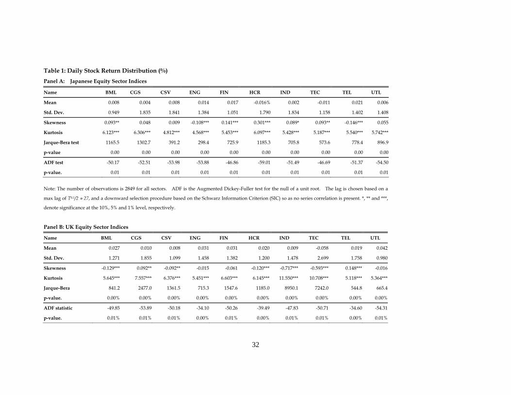
32

Note: The number of observations is 2849 for all sectors. ADF is the Augmented Dickey-Fuller test for the null of a unit root. The lag is chosen based on a

max lag of T0.5/2 27, and a downward selection procedure based on the Schwarz Information Criterion (SIC) so as no series correlation is present. *, ** and ***,

denote significance at the 10%, 5% and 1% level, respectively.

Panel B: UK Equity Sector Indices

Name BML CGS CSV ENG FIN HCR IND TEC TEL UTL

Mean 0.027 0.010 0.008 0.031 0.031 0.020 0.009 -0.058 0.019 0.042

Std. Dev. 1.271 1.855 1.099 1.458 1.382 1.200 1.478 2.699 1.758 0.980

Skewness -0.129*** 0.092** -0.092** -0.015 -0.061 -0.120*** -0.717*** -0.593*** 0.148*** -0.016

Kurtosis 5.645*** 7.557*** 6.376*** 5.451*** 6.603*** 6.145*** 11.550*** 10.708*** 5.118*** 5.364***

Jarque-Bera 841.2 2477.0 1361.5 715.3 1547.6 1185.0 8950.1 7242.0 544.8 665.4

p-value. 0.00% 0.00% 0.00% 0.00% 0.00% 0.00% 0.00% 0.00% 0.00% 0.00%

ADF statistic -49.85 -53.89 -50.18 -34.10 -50.26 -39.49 -47.83 -50.71 -34.60 -54.31

p-value. 0.01% 0.01% 0.01% 0.00% 0.01% 0.00% 0.01% 0.01% 0.00% 0.01%

Table 1: Daily Stock Return Distribution (%)

Panel A: Japanese Equity Sector Indices

Name BML CGS CSV ENG FIN HCR IND TEC TEL UTL

Mean 0.008 0.004 0.008 0.014 0.017 -0.016% 0.002 -0.011 0.021 0.006

Std. Dev. 0.949 1.835 1.841 1.384 1.051 1.790 1.834 1.158 1.402 1.408

Skewness 0.093** 0.048 0.009 -0.108*** 0.141*** 0.301*** 0.089* 0.093** -0.146*** 0.055

Kurtosis 6.123*** 6.306*** 4.812*** 4.568*** 5.453*** 6.097*** 5.428*** 5.187*** 5.540*** 5.742***

Jarque-Bera test 1165.5 1302.7 391.2 298.4 725.9 1185.3 705.8 573.6 778.4 896.9

p-value 0.00 0.00 0.00 0.00 0.00 0.00 0.00 0.00 0.00 0.00

ADF test -50.17 -52.51 -53.98 -53.88 -46.86 -59.01 -51.49 -46.69 -51.37 -54.50

p-value. 0.01 0.01 0.01 0.01 0.01 0.01 0.01 0.01 0.01 0.01

33

Table 1: Daily Stock Return Distribution (CONT’D)

Panel C: US Equity Sector Indices

Name BML CGS CSV ENG FIN HCR IND TEC TEL UTL

Mean 0.027 0.010 0.027 0.046 0.041 0.027 0.033 0.030 0.014 0.019

Std. Dev. 1.369 1.267 1.256 1.415 1.353 1.050 1.278 2.015 1.325 1.110

Skewness 0.083* -0.251*** -0.186*** -0.023 0.114*** -0.154*** -0.136*** 0.223*** -0.119*** -0.405***

Kurtosis 6.318*** 9.006*** 8.554*** 4.860*** 6.446*** 8.347*** 7.415*** 6.847*** 6.039*** 10.214***

Jarque-Bera 1314.4 4325.5 3690.2 412.1 1420.2 3416.3 2330.5 1785.9 1106.3 6275.0

p-value. 0.00% 0.00% 0.00% 0.00% 0.00% 0.00% 0.00% 0.00% 0.00% 0.00%

ADF statistic -52.51 -54.88 -38.94 -40.38 -51.60 -34.40 -39.68 -54.04 -54.61 -51.13

p-value. 0.01% 0.01% 0.00% 0.00% 0.01% 0.00% 0.00% 0.01% 0.01% 0.01%

Panel D: National Equity Market Indices

Name Japan UK US

Mean 0.002 0.020 0.028

Std. Dev. 1.224 0.990 1.094

Skewness -0.075 -0.285*** -0.105***

Kurtosis 4.998*** 5.975*** 6.474***

Jarque-Bera 483.8 1105.8 1459.3

p-value 0.00% 0.00% 0.00%

ADF Statistic -52.5 -52.9 -54.4

p-value 0.00% 0.00% 0.00%

See note in Panel A

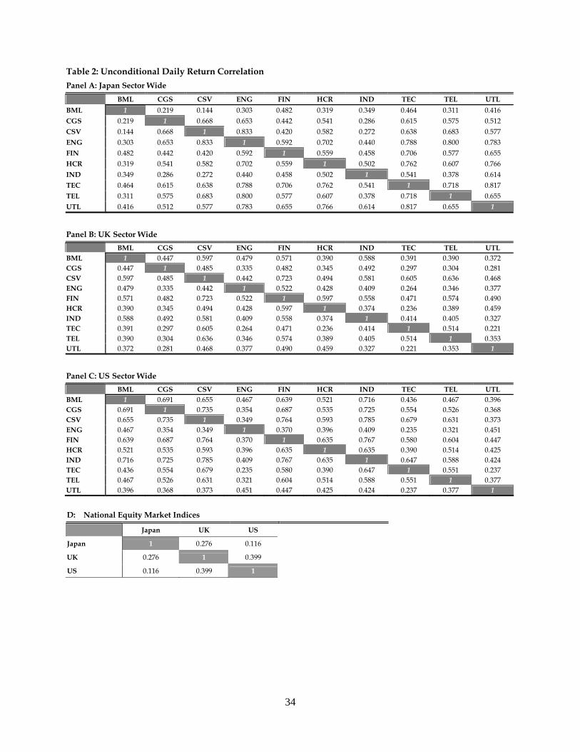
34

Table 2: Unconditional Daily Return Correlation Panel A: Japan Sector Wide

BML CGS CSV ENG FIN HCR IND TEC TEL UTL

BML 1 0.219 0.144 0.303 0.482 0.319 0.349 0.464 0.311 0.416 CGS 0.219 1 0.668 0.653 0.442 0.541 0.286 0.615 0.575 0.512 CSV 0.144 0.668 1 0.833 0.420 0.582 0.272 0.638 0.683 0.577 ENG 0.303 0.653 0.833 1 0.592 0.702 0.440 0.788 0.800 0.783 FIN 0.482 0.442 0.420 0.592 1 0.559 0.458 0.706 0.577 0.655 HCR 0.319 0.541 0.582 0.702 0.559 1 0.502 0.762 0.607 0.766

IND 0.349 0.286 0.272 0.440 0.458 0.502 1 0.541 0.378 0.614 TEC 0.464 0.615 0.638 0.788 0.706 0.762 0.541 1 0.718 0.817 TEL 0.311 0.575 0.683 0.800 0.577 0.607 0.378 0.718 1 0.655 UTL 0.416 0.512 0.577 0.783 0.655 0.766 0.614 0.817 0.655 1

Panel B: UK Sector Wide

BML CGS CSV ENG FIN HCR IND TEC TEL UTL BML 1 0.447 0.597 0.479 0.571 0.390 0.588 0.391 0.390 0.372 CGS 0.447 1 0.485 0.335 0.482 0.345 0.492 0.297 0.304 0.281 CSV 0.597 0.485 1 0.442 0.723 0.494 0.581 0.605 0.636 0.468 ENG 0.479 0.335 0.442 1 0.522 0.428 0.409 0.264 0.346 0.377 FIN 0.571 0.482 0.723 0.522 1 0.597 0.558 0.471 0.574 0.490 HCR 0.390 0.345 0.494 0.428 0.597 1 0.374 0.236 0.389 0.459 IND 0.588 0.492 0.581 0.409 0.558 0.374 1 0.414 0.405 0.327 TEC 0.391 0.297 0.605 0.264 0.471 0.236 0.414 1 0.514 0.221 TEL 0.390 0.304 0.636 0.346 0.574 0.389 0.405 0.514 1 0.353 UTL 0.372 0.281 0.468 0.377 0.490 0.459 0.327 0.221 0.353 1

Panel C: US Sector Wide

BML CGS CSV ENG FIN HCR IND TEC TEL UTL BML 1 0.691 0.655 0.467 0.639 0.521 0.716 0.436 0.467 0.396 CGS 0.691 1 0.735 0.354 0.687 0.535 0.725 0.554 0.526 0.368 CSV 0.655 0.735 1 0.349 0.764 0.593 0.785 0.679 0.631 0.373 ENG 0.467 0.354 0.349 1 0.370 0.396 0.409 0.235 0.321 0.451 FIN 0.639 0.687 0.764 0.370 1 0.635 0.767 0.580 0.604 0.447 HCR 0.521 0.535 0.593 0.396 0.635 1 0.635 0.390 0.514 0.425 IND 0.716 0.725 0.785 0.409 0.767 0.635 1 0.647 0.588 0.424 TEC 0.436 0.554 0.679 0.235 0.580 0.390 0.647 1 0.551 0.237 TEL 0.467 0.526 0.631 0.321 0.604 0.514 0.588 0.551 1 0.377 UTL 0.396 0.368 0.373 0.451 0.447 0.425 0.424 0.237 0.377 1

D: National Equity Market Indices

Japan UK US

Japan 1 0.276 0.116

UK 0.276 1 0.399

US 0.116 0.399 1

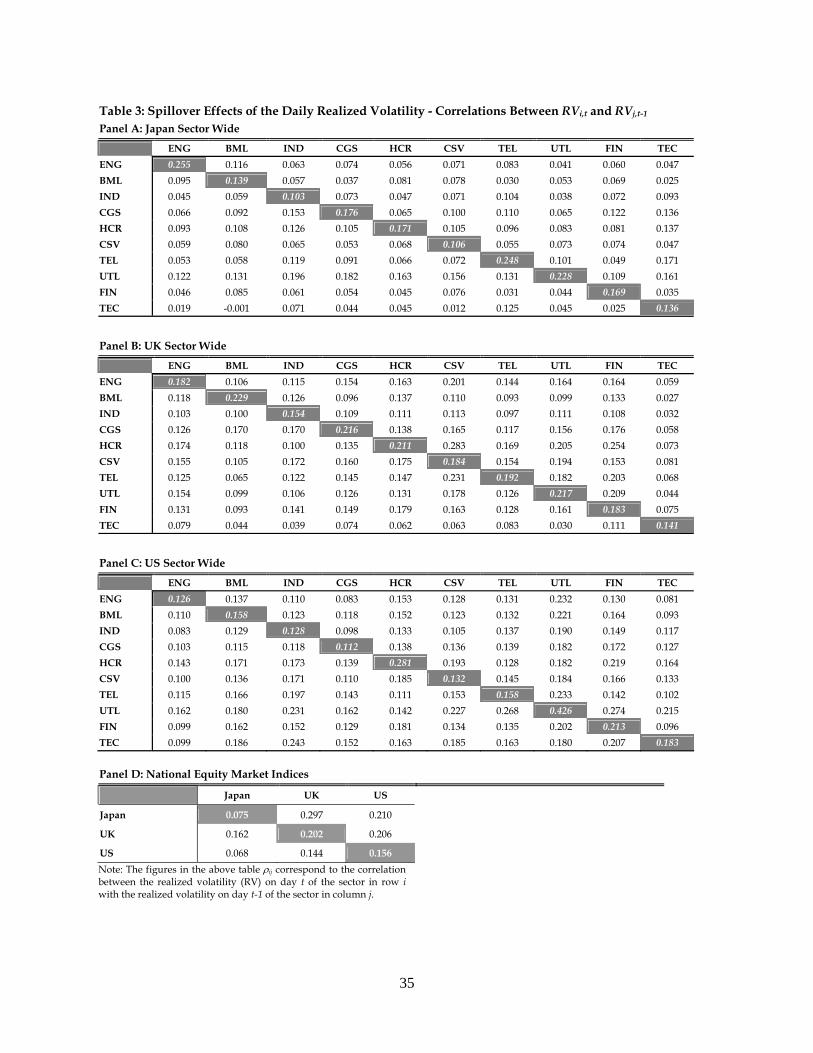
35

Table 3: Spillover Effects of the Daily Realized Volatility - Correlations Between RVi,t and RVj,t-1 Panel A: Japan Sector Wide

ENG BML IND CGS HCR CSV TEL UTL FIN TEC

ENG 0.255 0.116 0.063 0.074 0.056 0.071 0.083 0.041 0.060 0.047

BML 0.095 0.139 0.057 0.037 0.081 0.078 0.030 0.053 0.069 0.025

IND 0.045 0.059 0.103 0.073 0.047 0.071 0.104 0.038 0.072 0.093

CGS 0.066 0.092 0.153 0.176 0.065 0.100 0.110 0.065 0.122 0.136

HCR 0.093 0.108 0.126 0.105 0.171 0.105 0.096 0.083 0.081 0.137

CSV 0.059 0.080 0.065 0.053 0.068 0.106 0.055 0.073 0.074 0.047

TEL 0.053 0.058 0.119 0.091 0.066 0.072 0.248 0.101 0.049 0.171

UTL 0.122 0.131 0.196 0.182 0.163 0.156 0.131 0.228 0.109 0.161

FIN 0.046 0.085 0.061 0.054 0.045 0.076 0.031 0.044 0.169 0.035

TEC 0.019 -0.001 0.071 0.044 0.045 0.012 0.125 0.045 0.025 0.136

Panel B: UK Sector Wide

ENG BML IND CGS HCR CSV TEL UTL FIN TEC

ENG 0.182 0.106 0.115 0.154 0.163 0.201 0.144 0.164 0.164 0.059

BML 0.118 0.229 0.126 0.096 0.137 0.110 0.093 0.099 0.133 0.027

IND 0.103 0.100 0.154 0.109 0.111 0.113 0.097 0.111 0.108 0.032

CGS 0.126 0.170 0.170 0.216 0.138 0.165 0.117 0.156 0.176 0.058

HCR 0.174 0.118 0.100 0.135 0.211 0.283 0.169 0.205 0.254 0.073

CSV 0.155 0.105 0.172 0.160 0.175 0.184 0.154 0.194 0.153 0.081

TEL 0.125 0.065 0.122 0.145 0.147 0.231 0.192 0.182 0.203 0.068

UTL 0.154 0.099 0.106 0.126 0.131 0.178 0.126 0.217 0.209 0.044

FIN 0.131 0.093 0.141 0.149 0.179 0.163 0.128 0.161 0.183 0.075

TEC 0.079 0.044 0.039 0.074 0.062 0.063 0.083 0.030 0.111 0.141

Panel C: US Sector Wide

ENG BML IND CGS HCR CSV TEL UTL FIN TEC

ENG 0.126 0.137 0.110 0.083 0.153 0.128 0.131 0.232 0.130 0.081

BML 0.110 0.158 0.123 0.118 0.152 0.123 0.132 0.221 0.164 0.093

IND 0.083 0.129 0.128 0.098 0.133 0.105 0.137 0.190 0.149 0.117

CGS 0.103 0.115 0.118 0.112 0.138 0.136 0.139 0.182 0.172 0.127

HCR 0.143 0.171 0.173 0.139 0.281 0.193 0.128 0.182 0.219 0.164

CSV 0.100 0.136 0.171 0.110 0.185 0.132 0.145 0.184 0.166 0.133

TEL 0.115 0.166 0.197 0.143 0.111 0.153 0.158 0.233 0.142 0.102

UTL 0.162 0.180 0.231 0.162 0.142 0.227 0.268 0.426 0.274 0.215

FIN 0.099 0.162 0.152 0.129 0.181 0.134 0.135 0.202 0.213 0.096

TEC 0.099 0.186 0.243 0.152 0.163 0.185 0.163 0.180 0.207 0.183

Panel D: National Equity Market Indices

Japan UK US

Japan 0.075 0.297 0.210

UK 0.162 0.202 0.206

US 0.068 0.144 0.156

Note: The figures in the above table ij correspond to the correlation between the realized volatility (RV) on day t of the sector in row i with the realized volatility on day t-1 of the sector in column j.

36

Table 4: In-sample MGARCH Estimation The Table below shows the parameters estimated from the MGARCH models. The sample period is from July/1/1996 to June/28/2002. The “a” is the parameter of the ARCH factor in the second step of the DCC-type MGARCH model; the “b” is the parameter of the GARCH factor in the second step of the DCC-type MGARCH model; the “g” is the parameter of the asymmetry effect in the second step of the DCC-type MGARCH model estimation. The structure break is on the date: Jan/1/1999. Panel A-1: Domestic Sector Portfolio of the Japanese Equity Market

Without Structure Break

Series Diagonal Models a^2 b^2 g^2

ENG DCC 0.011 *** 0.986 ***

ADCC 0.012 *** 0.984 *** 0.000 ***

BML DCC 0.021 *** 0.972 ***

ADCC 0.020 *** 0.971 *** 0.006 ***

IND DCC 0.025 *** 0.957 ***

ADCC 0.024 *** 0.956 *** 0.005 ***

CGS DCC 0.017 *** 0.969 ***

ADCC 0.020 *** 0.966 *** 0.000 ***

HCR DCC 0.016 *** 0.982 ***

ADCC 0.017 *** 0.982 *** 0.000 ***

CSV DCC 0.019 *** 0.967 ***

ADCC 0.020 *** 0.965 *** 0.001 ***

TEL DCC 0.019 *** 0.954 ***

ADCC 0.017 *** 0.954 *** 0.005 ***

UTL DCC 0.005 *** 0.987 ***

ADCC 0.006 *** 0.986 *** 0.000 ***

FIN DCC 0.031 *** 0.951 ***

ADCC 0.030 *** 0.947 *** 0.010 ***

TEC DCC 0.025 *** 0.954 ***

ADCC 0.023 *** 0.954 *** 0.004 ***

Scalar Models a b g

DCC 0.016 *** 0.976 ***

ADCC 0.016 *** 0.976 *** 0.000 ***

The "*"s indicate the parameter significance level: *** -- 99%, ** -- 95%, * -- 90%. The "-" means the parameter is not significant at 90% confidence level.

37

Table 4: In-sample MGARCH-Type Model Estimation Results (CONT’D) Panel A-2: Domestic Sector Portfolio of the Japanese Equity Market (CONT’D)

With Structure Break Period 1 Period 2

Series Diagonal Models a^2 b^2 g^2 a^2 b^2 g^2

ENG DCC 0.014 *** 0.829 *** 0.009 *** 0.981 ***

ADCC 0.013 *** 0.818 *** 0.009 *** 0.009 *** 0.988 *** 0.000 ***

BML DCC 0.057 *** 0.739 *** 0.033 *** 0.903 ***

ADCC 0.041 *** 0.734 *** 0.050 *** 0.031 *** 0.910 *** 0.003 ***

IND DCC 0.027 *** 0.760 *** 0.035 *** 0.907 ***

ADCC 0.021 *** 0.675 *** 0.025 *** 0.034 *** 0.909 *** 0.006 ***

CGS DCC 0.015 *** 0.797 *** 0.017 *** 0.924 ***

ADCC 0.008 *** 0.698 *** 0.037 *** 0.020 *** 0.914 *** 0.000 ***

HCR DCC 0.010 *** 0.775 *** 0.015 *** 0.973 ***

ADCC 0.007 *** 0.722 *** 0.012 *** 0.015 *** 0.965 *** 0.020 ***

CSV DCC 0.030 *** 0.697 *** 0.025 *** 0.921 ***

ADCC 0.028 *** 0.721 *** 0.011 *** 0.028 *** 0.914 *** 0.000 ***

TEL DCC 0.012 *** 0.857 *** 0.042 *** 0.868 ***

ADCC 0.012 *** 0.849 *** 0.007 *** 0.040 *** 0.879 *** 0.004 ***

UTL DCC 0.016 *** 0.984 *** 0.006 *** 0.973 ***

ADCC 0.023 *** 0.977 *** 0.000 *** 0.014 *** 0.753 - 0.029 -

FIN DCC 0.083 *** 0.779 *** 0.074 *** 0.797 ***

ADCC 0.064 *** 0.767 *** 0.050 *** 0.064 *** 0.818 *** 0.006 **

TEC DCC 0.048 *** 0.721 *** 0.042 *** 0.891 ***

ADCC 0.037 *** 0.439 *** 0.137 *** 0.041 *** 0.891 *** 0.006 ***

Scalar Models a b g a b g

DCC 0.017 *** 0.924 *** 0.022 *** 0.932 ***

ADCC 0.017 *** 0.924 *** 0.000 - 0.022 *** 0.932 *** 0.000 -

The "*"s indicates the parameter's significance level: *** -- 99%, ** -- 95%, * -- 90%.

Panel A-3: Summary Table for Domestic Sector Portfolio of the Japanese Equity Market

Scalar Models Diagonal Models

LLF Num. of Para AIC SIC LLF Num. of Para AIC SIC

CCC 50134*** 75 128.36 530.03 DCC 50657*** 50 78.33 346.12

DCC 50614*** 32 42.34 213.72 ADCC 50663*** 60 98.33 419.67

ADCC 50616*** 33 44.34 221.07 DCC-break 50911*** 70 118.32 493.22

DCC-break 50847*** 34 46.33 228.42 ADCC-break 50930 90 158.32 640.33

ADCC-break 50847*** 36 50.33 243.13

Note: The LLF is the log-likelihood value; the AIC is the Akaike Information Criterion, AIC = 2 x K – 2 x ln(LLF), where K is the number of parameter; the SIC is the Schwarz Information Criterion, SIC = K x ln(LLF) - 2 x ln(LLF). The "*"s indicate the significance level of the LR test, with the highest LLF estimator as unrestricted control model: *** -- 99%, ** -- 95%, * -- 90%. BEKK models are not included in the LR test as they are not nested with the conditional correlation specifications. The test statistics is 2 x [LLFunrestricticed – LLFrestricted], the critical value is drawn from the chi-square distribution with degree of freedom equals to the number of restricted parameters.

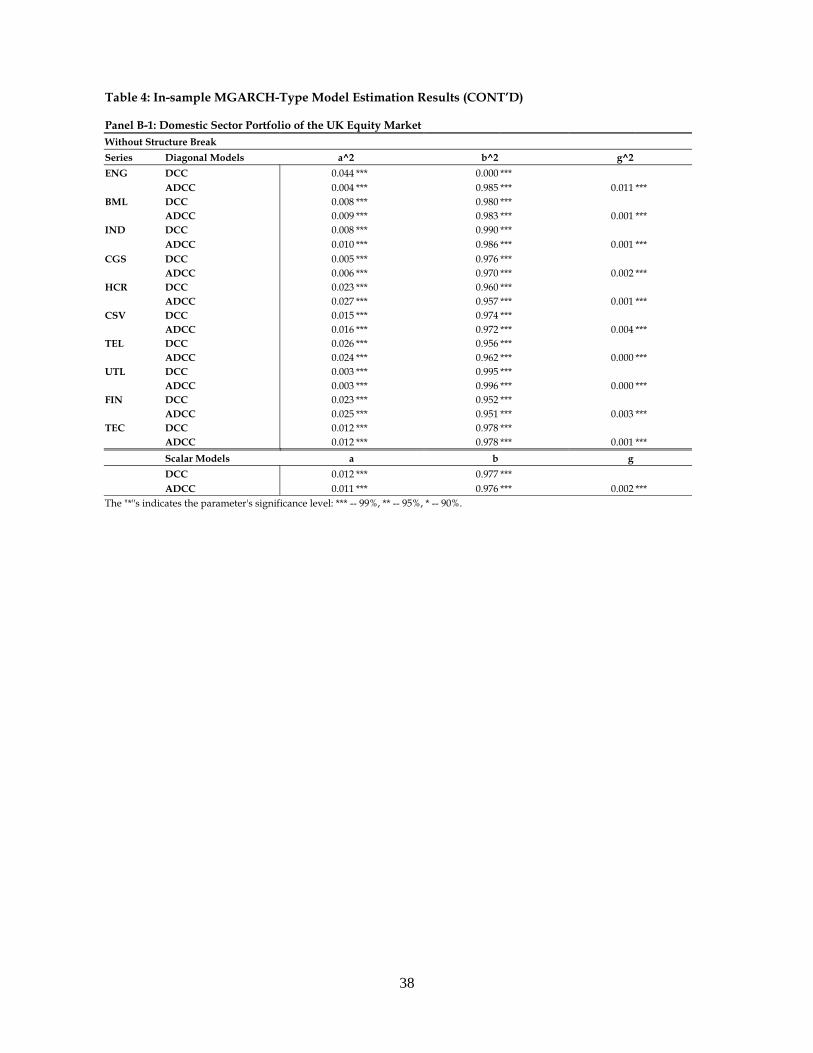
38

Table 4: In-sample MGARCH-Type Model Estimation Results (CONT’D) Panel B-1: Domestic Sector Portfolio of the UK Equity Market Without Structure Break

Series Diagonal Models a^2 b^2 g^2

ENG DCC 0.044 *** 0.000 *** ADCC 0.004 *** 0.985 *** 0.011 *** BML DCC 0.008 *** 0.980 *** ADCC 0.009 *** 0.983 *** 0.001 *** IND DCC 0.008 *** 0.990 *** ADCC 0.010 *** 0.986 *** 0.001 *** CGS DCC 0.005 *** 0.976 *** ADCC 0.006 *** 0.970 *** 0.002 *** HCR DCC 0.023 *** 0.960 *** ADCC 0.027 *** 0.957 *** 0.001 *** CSV DCC 0.015 *** 0.974 *** ADCC 0.016 *** 0.972 *** 0.004 *** TEL DCC 0.026 *** 0.956 *** ADCC 0.024 *** 0.962 *** 0.000 *** UTL DCC 0.003 *** 0.995 *** ADCC 0.003 *** 0.996 *** 0.000 *** FIN DCC 0.023 *** 0.952 *** ADCC 0.025 *** 0.951 *** 0.003 *** TEC DCC 0.012 *** 0.978 *** ADCC 0.012 *** 0.978 *** 0.001 ***

Scalar Models a b g

DCC 0.012 *** 0.977 *** ADCC 0.011 *** 0.976 *** 0.002 *** The "*"s indicates the parameter's significance level: *** -- 99%, ** -- 95%, * -- 90%.

39

Table 4: In-sample MGARCH-Type Model Estimation Results (CONT’D) Panel B-2: Domestic Sector Portfolio of the UK Equity Market (CONT’D)

With Structure Break Period 1 Period 2

Series Diagonal Models a^2 b^2 g^2 a^2 b^2 g^2

ENG DCC 0.002 *** 0.000 *** 0.044 *** 0.000 *** ADCC 0.000 *** 0.851 *** 0.048 *** 0.047 *** 0.000 *** 0.363 *** BML DCC 0.018 *** 0.501 *** 0.006 *** 0.981 *** ADCC 0.005 *** 0.901 *** 0.032 *** 0.005 *** 0.981 *** 0.004 *** IND DCC 0.023 *** 0.438 *** 0.010 *** 0.971 *** ADCC 0.006 *** 0.915 *** 0.058 *** 0.010 *** 0.968 *** 0.000 *** CGS DCC 0.041 *** 0.400 *** 0.004 *** 0.963 *** ADCC 0.016 *** 0.816 *** 0.038 *** 0.009 *** 0.883 *** 0.000 *** HCR DCC 0.023 *** 0.958 *** 0.009 *** 0.991 *** ADCC 0.015 *** 0.890 *** 0.041 *** 0.010 *** 0.990 *** 0.000 *** CSV DCC 0.065 *** 0.101 - 0.024 *** 0.952 *** ADCC 0.005 *** 0.725 *** 0.144 *** 0.025 *** 0.943 *** 0.012 *** TEL DCC 0.051 *** 0.766 *** 0.034 *** 0.942 *** ADCC 0.080 *** 0.875 *** 0.020 *** 0.044 *** 0.932 *** 0.000 *** UTL DCC 0.010 *** 0.000 *** 0.002 *** 0.960 *** ADCC 0.002 *** 0.000 *** 0.000 *** 0.002 *** 0.957 *** 0.000 *** FIN DCC 0.110 *** 0.072 - 0.021 *** 0.948 *** ADCC 0.020 *** 0.919 *** 0.034 *** 0.020 *** 0.946 *** 0.005 *** TEC DCC 0.006 *** 0.875 *** 0.014 *** 0.969 *** ADCC 0.003 *** 0.996 *** 0.001 *** 0.015 *** 0.959 *** 0.002 ***

Scalar Models a b g a b g DCC 0.017 *** 0.911 *** 0.011 *** 0.972 *** ADCC 0.009 *** 0.922 *** 0.015 *** 0.011 *** 0.972 *** 0.000 - The "*"s indicates the parameter's significance level: *** -- 99%, ** -- 95%, * -- 90%.

Panel B-3: Summary Table for Domestic Sector Portfolio of the UK Equity Market

Scalar Models Diagonal Models

LLF Num. of Para AIC SIC LLF Num. of Para AIC SIC CCC 47311*** 75 128.47 530.144 DCC 47562*** 50 78.46 346.24 DCC 47547*** 32 42.46 213.84 ADCC 47595*** 60 98.46 419.80 ADCC 47574*** 33 44.46 221.20 DCC-break 47736*** 70 118.45 493.35 DCC-break 47704*** 34 46.45 228.55 ADCC-break 47766 90 158.45 640.46 ADCC-break 47708*** 36 50.45 243.26 Note: The LLF is the log-likelihood value; the AIC is the Akaike Information Criterion, AIC = 2 x K – 2 x ln(LLF), where K is the number of parameter; the SIC is the Schwarz Information Criterion, SIC = K x ln(LLF) - 2 x ln(LLF). The "*"s indicate the significance level of the LR test, with the highest LLF estimator as unrestricted control model: *** -- 99%, ** -- 95%, * -- 90%. BEKK models are not included in the LR test as they are not nested with the conditional correlation specifications. The test statistics is 2 x [LLFunrestricticed – LLFrestricted], the critical value is drawn from the chi-square distribution with degree of freedom equals to the number of restricted parameters.

40

Table 4: In-sample MGARCH-Type Model Estimation Results (CONT’D) Panel C-1: Domestic Sector Portfolio of the US Equity Market

Without Structure Break

Series Diagonal Models a^2 b^2 g^2

ENG BEKK 0.025 *** 0.980 ***

DCC 0.006 *** 0.982 ***

ADCC 0.006 *** 0.983 *** 0.000 ***

BML BEKK 0.019 *** 0.980 ***

DCC 0.026 *** 0.956 ***

ADCC 0.021 *** 0.956 *** 0.018 ***

IND BEKK 0.029 *** 0.969 ***

DCC 0.021 *** 0.970 ***

ADCC 0.019 *** 0.964 *** 0.013 ***

CGS BEKK 0.021 *** 0.974 ***

DCC 0.022 *** 0.960 ***

ADCC 0.017 *** 0.958 *** 0.015 ***

HCR BEKK 0.031 *** 0.960 ***

DCC 0.013 *** 0.987 ***

ADCC 0.013 *** 0.984 *** 0.004 ***

CSV BEKK 0.029 *** 0.968 ***

DCC 0.015 *** 0.979 ***

ADCC 0.012 *** 0.980 *** 0.008 ***

TEL BEKK 0.025 *** 0.966 ***

DCC 0.007 *** 0.988 ***

ADCC 0.007 *** 0.990 *** 0.000 ***

UTL BEKK 0.036 - 0.960 ***

DCC 0.007 *** 0.988 ***

ADCC 0.009 *** 0.985 *** 0.000 ***

FIN BEKK 0.031 *** 0.965 ***

DCC 0.018 *** 0.971 ***

ADCC 0.016 *** 0.969 *** 0.006 ***

TEC BEKK 0.027 *** 0.966 ***

DCC 0.016 *** 0.974 ***

ADCC 0.015 *** 0.974 *** 0.004 ***

Scalar Models a b g

BEKK 0.146 *** 0.989 ***

DCC 0.014 *** 0.979 *** `

ADCC 0.014 *** 0.979 *** 0.000 -

The "*"s indicates the parameter's significance level: *** -- 99%, ** -- 95%, * -- 90%.

41

Table 4: In-sample MGARCH-Type Model Estimation Results (CONT’D) Panel C-2: Domestic Sector Portfolio of the US Equity Market (CONT’D)

With Structure Break Period 1 Period 1

Series Diagonal Models a^2 b^2 g^2 a^2 b^2 g^2

ENG DCC 0.009 *** 0.839 *** 0.042 *** 0.479 ***

ADCC 0.009 *** 0.990 *** 0.001 *** 0.048 *** 0.480 *** 0.000 ***

BML DCC 0.017 *** 0.838 *** 0.025 *** 0.949 ***

ADCC 0.003 *** 0.982 *** 0.015 *** 0.018 *** 0.955 *** 0.019 ***

IND DCC 0.034 *** 0.826 *** 0.027 *** 0.941 ***

ADCC 0.006 *** 0.951 *** 0.021 *** 0.024 *** 0.935 *** 0.012 ***

CGS DCC 0.027 *** 0.758 *** 0.020 *** 0.956 ***

ADCC 0.004 *** 0.945 *** 0.027 *** 0.015 *** 0.952 *** 0.018 ***

HCR DCC 0.025 *** 0.851 *** 0.009 *** 0.991 ***

ADCC 0.009 *** 0.943 *** 0.014 *** 0.010 *** 0.990 *** 0.000 ***

CSV DCC 0.020 *** 0.838 *** 0.018 *** 0.969 ***

ADCC 0.003 *** 0.955 *** 0.017 *** 0.014 *** 0.968 *** 0.017 ***

TEL DCC 0.015 *** 0.931 *** 0.006 *** 0.964 ***

ADCC 0.019 *** 0.859 *** 0.022 *** 0.013 *** 0.930 *** 0.000 ***

UTL DCC 0.023 *** 0.977 *** 0.023 *** 0.000 ***

ADCC 0.085 *** 0.708 *** 0.000 *** 0.035 *** 0.011 *** 0.000 ***

FIN DCC 0.014 *** 0.899 *** 0.021 *** 0.953 ***

ADCC 0.001 *** 0.931 *** 0.064 *** 0.021 *** 0.950 *** 0.003 ***

TEC DCC 0.048 *** 0.800 *** 0.014 *** 0.967 ***

ADCC 0.007 *** 0.915 *** 0.059 *** 0.014 *** 0.964 *** 0.006 ***

Scalar Models a b g a b g

DCC 0.018 *** 0.916 *** 0.015 *** 0.963 ***

ADCC 0.008 *** 0.939 *** 0.013 *** 0.015 *** 0.963 *** 0.000 -

The "*"s indicates the parameter's significance level: *** -- 99%, ** -- 95%, * -- 90%.

Panel C-3: Summary Table for Domestic Sector Portfolio of the US Equity Market

Scalar Models Diagonal Models

LLF Num. of Para AIC SIC LLF Num. of Para AIC SIC

BEKK 49733 47 72.37 324.09 BEKK 49747 65 108.37 456.49

CCC 49472*** 75 128.38 530.06 DCC 49907*** 50 78.36 346.15

DCC 49867*** 32 42.37 213.75 ADCC 49917*** 60 98.36 419.70

ADCC 49868*** 33 44.37 221.10 DCC-break 50084*** 70 118.36 493.25

DCC-break 50050*** 34 46.36 228.45 ADCC-break 50131 90 158.36 640.36

ADCC-break 50055*** 36 50.36 243.16 Note: The LLF is the log-likelihood value; the AIC is the Akaike Information Criterion, AIC = 2 x K – 2 x ln(LLF), where K is the number of parameter; the SIC is the Schwarz Information Criterion, SIC = K x ln(LLF) - 2 x ln(LLF). The "*"s indicate the significance level of the LR test, with the highest LLF estimator as unrestricted control model: *** -- 99%, ** -- 95%, * -- 90%. BEKK models are not included in the LR test as they are not nested with the conditional correlation specifications. The test statistics is 2 x [LLFunrestricticed – LLFrestricted], the critical value is drawn from the chi-square distribution with degree of freedom equals to the number of restricted parameters

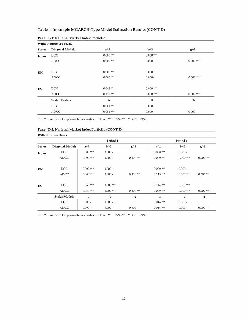
42

Table 4: In-sample MGARCH-Type Model Estimation Results (CONT’D) Panel D-1: National Market Index Portfolio

Without Structure Break

Series Diagonal Models a^2 b^2 g^2

Japan DCC 0.000 *** 0.000 ***

ADCC 0.000 *** 0.000 - 0.000 ***

UK DCC 0.000 *** 0.000 -

ADCC 0.000 *** 0.000 - 0.000 ***

US DCC 0.042 *** 0.000 ***

ADCC 0.122 *** 0.000 *** 0.000 ***

Scalar Models A B G

DCC 0.001 *** 0.000 -

ADCC 0.001 *** 0.000 - 0.000 -

The "*"s indicates the parameter's significance level: *** -- 99%, ** -- 95%, * -- 90%.

Panel D-2: National Market Index Portfolio (CONT’D)

With Structure Break

Period 1 Period 1

Series Diagonal Models a^2 b^2 g^2 a^2 b^2 g^2

Japan DCC 0.000 *** 0.000 - 0.000 *** 0.000 -

ADCC 0.000 *** 0.000 - 0.000 *** 0.000 *** 0.000 *** 0.000 ***

UK DCC 0.000 *** 0.000 - 0.000 *** 0.000 -

ADCC 0.000 *** 0.000 - 0.000 *** 0.115 *** 0.000 *** 0.000 ***

US DCC 0.063 *** 0.000 *** 0.144 *** 0.000 ***

ADCC 0.080 *** 0.000 *** 0.000 *** 0.000 *** 0.000 *** 0.000 ***

Scalar Models a b g a b g

DCC 0.000 - 0.000 - 0.016 *** 0.000 -

ADCC 0.000 - 0.000 - 0.000 - 0.016 *** 0.000 - 0.000 -

The "*"s indicates the parameter's significance level: *** -- 99%, ** -- 95%, * -- 90%.

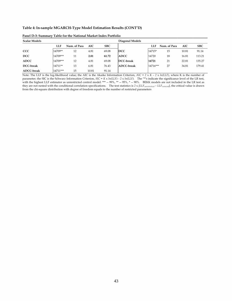
43

Table 4: In-sample MGARCH-Type Model Estimation Results (CONT’D) Panel D-3: Summary Table for the National Market Index Portfolio

Scalar Models Diagonal Models

LLF Num. of Para AIC SBC LLF Num. of Para AIC SBC

CCC 14709** 12 4.81 69.08 DCC 14715* 15 10.81 91.14

DCC 14709*** 11 2.81 61.72 ADCC 14720 18 16.81 113.21

ADCC 14709*** 12 4.81 69.08 DCC-break 14721 21 22.81 135.27

DCC-break 14711** 13 6.81 76.43 ADCC-break 14716*** 27 34.81 179.41

ADCC-break 14711*** 15 10.81 91.14 Note: The LLF is the log-likelihood value; the AIC is the Akaike Information Criterion, AIC = 2 x K – 2 x ln(LLF), where K is the number of parameter; the SIC is the Schwarz Information Criterion, SIC = K x ln(LLF) - 2 x ln(LLF). The "*"s indicate the significance level of the LR test, with the highest LLF estimator as unrestricted control model: *** -- 99%, ** -- 95%, * -- 90%. BEKK models are not included in the LR test as they are not nested with the conditional correlation specifications. The test statistics is 2 x [LLFunrestricticed – LLFrestricted], the critical value is drawn from the chi-square distribution with degree of freedom equals to the number of restricted parameters

44

Table 5: In-sample Portfolio Performance Comparison The Table below shows the performances of the portfolios based on estimated variance-covariance matrices of the different MGARCH models. All the portfolios are rebalanced on a monthly basis over the period from July/1/1996 to June/28/2002.

Panel A: Model Selection under the max-return strategy

Layer JP Equity Market UK Equity Market US Equity Market National Market Index

MGARCH Models μ(SR) μ(Ret) μ(Std) μ(U) μ(SR) μ(Ret) μ(Std) μ(U) μ(SR) μ(Ret) μ(Std) μ(U) μ(SR) μ(Ret) μ(Std) μ(U)

BEKK - - - - - - - - 2.5126 14.2350% 5.7882% 0.0313% - - - - diagonal BEKK - - - - - - - - 2.5358 14.1780% 5.7190% 0.1365% - - - - scalar CCC 2.4289 16.7490% 7.2835% -0.7119% 2.5770 13.7740% 5.4748% 0.3104% 2.4238 14.5180% 6.2416% -0.6644% 1.4695 7.1788% 5.0042% -5.1236%

scalar DCC 2.5381 16.2870% 6.5228% 0.2421% 2.6763 13.5490% 5.1490% 0.8418% 2.5148 14.3200% 5.7890% 0.0424% 1.4712 6.9242% 4.8533% -4.9949%

scalar ADCC 2.5383 16.2900% 6.5236% 0.2428% 2.6761 13.5930% 5.1654% 0.8448% 2.5149 14.3220% 5.7895% 0.0427% 1.4712 6.9242% 4.8533% -4.9949%

diagonal DCC 2.5480 16.2260% 6.4724% 0.2974% 2.6572 13.5370% 5.1881% 0.7310% 2.5251 14.3440% 5.7829% 0.0891% 1.4711 6.9249% 4.8542% -4.9960%

diagonal ADCC 2.5512 16.2220% 6.4599% 0.3229% 2.6737 13.5350% 5.1460% 0.8236% 2.5262 14.4140% 5.8084% 0.0955% 1.4709 6.9249% 4.8547% -4.9979%

scalar DCC-break 2.5490 16.3130% 6.4999% 0.3127% 2.6867 13.5590% 5.1290% 0.8928% 2.5369 14.3090% 5.7383% 0.1455% 1.4712 6.9377% 4.8549% -4.9890%

scalar ADCC-break 2.5490 16.3130% 6.4999% 0.3127% 2.6855 13.6310% 5.1562% 0.9002% 2.5343 14.4020% 5.7776% 0.1407% 1.4712 6.9377% 4.8549% -4.9890%

diagonal DCC-break 2.5575 16.3350% 6.4938% 0.3539% 2.6608 13.6540% 5.2267% 0.7552% 2.5265 14.3820% 5.8139% 0.0632% 1.4704 6.9368% 4.8578% -4.9966%

diagonal ADCC-break 2.5555 16.3620% 6.5094% 0.3389% 2.6784 13.5980% 5.1662% 0.8401% 2.5271 14.4880% 5.8361% 0.0905% 1.4705 6.9389% 4.8585% -4.9961%

Note: The Sharpe Ratio (SR), Utility (U) and average monthly portfolio return (Ret) and volatility (Std) are calculated from the portfolio constructed based on the maximum portfolio expected return with target variance strategy. The (SR) denotes the value of average monthly portfolio Sharpe-Ratio over the in-sample period; the (Ret) is the value of average monthly portfolio return; the (Std) is the value of average monthly portfolio standard deviation over the in-sample period; the (U) is the value of average monthly investor utility. “-“ indicates the particular MGARCH model is not suitable for the multivariate time-series data from the given portfolio. Bold indicates the best model under each model selection criteria.

45

Table 5: In-sample Portfolio Performance Comparison (CONT’D) The Table below shows the performances of the portfolios based on estimated variance-covariance matrices of the different MGARCH models. All the portfolios are rebalanced on a monthly basis over the period from July/1/1996 to June/28/2002.

Panel B: Model Selection under the min-variance Investment Strategy

Layer JP Equity Market UK Equity Market US Equity Market National Market Index

MGARCH Models μ(SR) μ(Ret) μ(Std) μ(U) μ(SR) μ(Ret) μ(Std) μ(U) μ(SR) μ(Ret) μ(Std) μ(U) μ(SR) μ(Ret) μ(Std) μ(U)

BEKK - - - - - - - - 4.5644 0.6500% 0.1488% 0.2837% - - - - diagonal BEKK - - - - - - - - 4.6065 0.6500% 0.1474% 0.2872% - - - - scalar CCC 3.8789 0.0800% 0.0222% 0.0259% 29.3080 0.4700% 0.0170% 0.4285% 4.4049 0.6500% 0.1554% 0.2685% 3.5868 0.5015% 0.2177% 0.0552%

scalar DCC 4.0533 0.0800% 0.0210% 0.0287% 30.4250 0.4700% 0.0163% 0.4301% 4.5701 0.6500% 0.1485% 0.2844% 3.5854 0.5015% 0.2176% 0.0553%

scalar ADCC 4.0535 0.0800% 0.0210% 0.0287% 30.4260 0.4700% 0.0163% 0.4301% 4.5702 0.6500% 0.1485% 0.2844% 3.5854 0.5015% 0.2176% 0.0553%

diagonal DCC 4.0690 0.0800% 0.0209% 0.0288% 30.2080 0.4700% 0.0164% 0.4298% 4.5889 0.6500% 0.1481% 0.2856% 3.5853 0.5015% 0.2176% 0.0553%

diagonal ADCC 4.0741 0.0800% 0.0209% 0.0289% 30.3970 0.4700% 0.0163% 0.4301% 4.5913 0.6500% 0.1480% 0.2858% 3.5850 0.5015% 0.2176% 0.0553%

scalar DCC-break 4.0706 0.0800% 0.0209% 0.0289% 30.5440 0.4700% 0.0162% 0.4302% 4.6104 0.6500% 0.1474% 0.2872% 3.5856 0.5015% 0.2170% 0.0558%

scalar ADCC-break 4.0706 0.0800% 0.0209% 0.0289% 30.5350 0.4700% 0.0162% 0.4302% 4.6064 0.6500% 0.1475% 0.2869% 3.5856 0.5015% 0.2170% 0.0558%

diagonal DCC-break 4.0842 0.0800% 0.0209% 0.0290% 30.2580 0.4700% 0.0164% 0.4298% 4.5919 0.6500% 0.1482% 0.2855% 3.5837 0.5015% 0.2172% 0.0554%

diagonal ADCC-break 4.0811 0.0800% 0.0209% 0.0290% 30.4550 0.4700% 0.0163% 0.4300% 4.5938 0.6500% 0.1481% 0.2857% 3.5841 0.5015% 0.2173% 0.0554%

See note in Panel A.

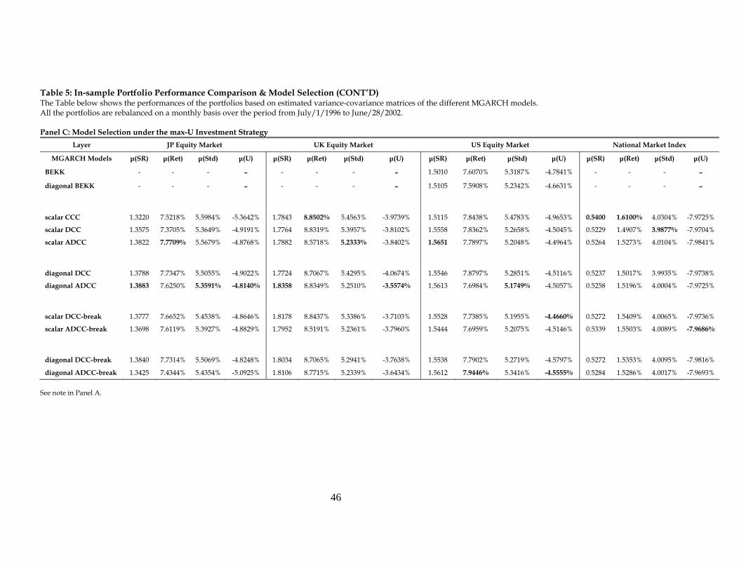
46

Table 5: In-sample Portfolio Performance Comparison & Model Selection (CONT’D) The Table below shows the performances of the portfolios based on estimated variance-covariance matrices of the different MGARCH models. All the portfolios are rebalanced on a monthly basis over the period from July/1/1996 to June/28/2002.

Panel C: Model Selection under the max-U Investment Strategy

Layer JP Equity Market UK Equity Market US Equity Market National Market Index

MGARCH Models μ(SR) μ(Ret) μ(Std) μ(U) μ(SR) μ(Ret) μ(Std) μ(U) μ(SR) μ(Ret) μ(Std) μ(U) μ(SR) μ(Ret) μ(Std) μ(U)

BEKK - - - - - - - - 1.5010 7.6070% 5.3187% -4.7841% - - - - diagonal BEKK - - - - - - - - 1.5105 7.5908% 5.2342% -4.6631% - - - - scalar CCC 1.3220 7.5218% 5.5984% -5.3642% 1.7843 8.8502% 5.4563% -3.9739% 1.5115 7.8438% 5.4783% -4.9653% 0.5400 1.6100% 4.0304% -7.9725%

scalar DCC 1.3575 7.3705% 5.3649% -4.9191% 1.7764 8.8319% 5.3957% -3.8102% 1.5558 7.8362% 5.2658% -4.5045% 0.5229 1.4907% 3.9877% -7.9704%

scalar ADCC 1.3822 7.7709% 5.5679% -4.8768% 1.7882 8.5718% 5.2333% -3.8402% 1.5651 7.7897% 5.2048% -4.4964% 0.5264 1.5273% 4.0104% -7.9841%

diagonal DCC 1.3788 7.7347% 5.5055% -4.9022% 1.7724 8.7067% 5.4295% -4.0674% 1.5546 7.8797% 5.2851% -4.5116% 0.5237 1.5017% 3.9935% -7.9738%

diagonal ADCC 1.3883 7.6250% 5.3591% -4.8140% 1.8358 8.8349% 5.2510% -3.5574% 1.5613 7.6984% 5.1749% -4.5057% 0.5258 1.5196% 4.0004% -7.9725%

scalar DCC-break 1.3777 7.6652% 5.4538% -4.8646% 1.8178 8.8437% 5.3386% -3.7103% 1.5528 7.7385% 5.1955% -4.4660% 0.5272 1.5409% 4.0065% -7.9736%

scalar ADCC-break 1.3698 7.6119% 5.3927% -4.8829% 1.7952 8.5191% 5.2361% -3.7960% 1.5444 7.6959% 5.2075% -4.5146% 0.5339 1.5503% 4.0089% -7.9686%

diagonal DCC-break 1.3840 7.7314% 5.5069% -4.8248% 1.8034 8.7065% 5.2941% -3.7638% 1.5538 7.7902% 5.2719% -4.5797% 0.5272 1.5353% 4.0095% -7.9816%

diagonal ADCC-break 1.3425 7.4344% 5.4354% -5.0925% 1.8106 8.7715% 5.2339% -3.6434% 1.5612 7.9446% 5.3416% -4.5555% 0.5284 1.5286% 4.0017% -7.9693%

See note in Panel A.

47

Table 5: In-sample Portfolio Performance Comparison & Model Selection (CONT’D) The Table below shows the selected models for each sub-portfolio under the different model selection criteria. The portfolios are derived based on estimated variance-covariance matrices of the different MGARCH models. Panel D: Best Performing Model across Selection Criteria

Investment Strategy max-return min-variance max-U

Layer μ(SR) μ(Ret) μ(Std) μ(U) μ(SR) μ(Std) μ(SR) μ(Ret) μ(Std) μ(U)

JP Equity Market diagonal

DCC-break CCC diagonal ADCC

diagonal DCC-break

diagonal DCC-break

diagonal DCC-break

diagonal ADCC scalar ADCC

diagonal ADCC

diagonal ADCC

UK Equity Market scalar DCC-break CCC scalar

DCC-break scalar

ADCC-break scalar

DCC-break scalar

DCC-break diagonal ADCC CCC scalar ADCC diagonal

ADCC

US Equity Market scalar

DCC-break CCC diagonal

BEKK scalar

DCC-break scalar

DCC-break scalar

DCC-break scalar ADCC diagonal

ADCC-break diagonal ADCC

scalar DCC-break

National Market Index scalar DCC CCC scalar DCC scalar DCC-break CCC scalar

DCC-break CCC

CCC

scalar DCC

scalar ADCC-break

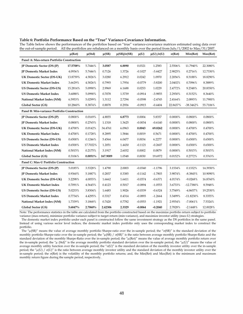
48

Table 6: Portfolio Performance Based on the “True” Variance-Covariance Information. The Table below shows the performances of the portfolios based on “true” variance-covariance matrices estimated using data over the out-of-sample period. All the portfolios are rebalanced on a monthly basis over the period from July/1/2002 to May/31/2007.

μ(Ret) μ(Std) μ(SR) μ(SR)/σ(SR) μ(U) μ(U) /σ(U) σ(Ret) Min(Ret) Max(Ret)

Panel A: Max-return Portfolio Construction JP Domestic Sector (DS-JP) 17.5708% 5.7446% 3.0587 6.8890 0.0321 1.2583 2.5506% 11.7940% 22.3080%

JP Domestic Market Index 4.0936% 5.7446% 0.7126 1.3726 -0.1027 -3.4427 2.9825% 0.2716% 12.7330%

UK Domestic Sector (DS-UK) 13.8759% 4.5826% 3.0280 6.2912 0.0242 1.0970 2.2056% 8.5188% 18.8290%

UK Domestic Market Index 3.6629% 4.5826% 0.7993 1.7954 -0.0779 -3.8200 2.0402% 0.7096% 8.3889%

US Domestic Sector (DS-US) 15.2814% 5.0990% 2.9969 6.1688 0.0253 1.0229 2.4772% 9.2348% 20.8350%

US Domestic Market Index 3.6088% 5.0990% 0.7078 1.5739 -0.0914 -3.9855 2.2930% 0.3152% 8.3640%

National Market Index (NM) 6.5953% 5.0299% 1.3112 2.7294 -0.0598 -2.4745 2.4164% 2.0893% 11.7900%

Global Sector (GS) 10.2860% 8.3874% 0.8878 0.2936 -0.0915 -0.4404 22.8437% -38.3462% 55.7106%

Panel B: Min-variance Portfolio Construction JP Domestic Sector (DS-JP) 0.0800% 0.0169% 4.8855 6.8773 0.0004 5.8357 0.0000% 0.0800% 0.0800%

JP Domestic Market Index 0.0800% 0.2765% 1.1318 1.3625 -0.0034 -0.6140 0.0000% 0.0800% 0.0800%

UK Domestic Sector (DS-UK) 0.4700% 0.0142% 34.4761 6.0963 0.0043 69.8262 0.0000% 0.4700% 0.4700%

UK Domestic Market Index 0.4700% 0.1728% 8.2895 1.5846 0.0019 0.5671 0.0000% 0.4700% 0.4700%

US Domestic Sector (DS-US) 0.6500% 0.1246% 5.4564 6.0477 0.0034 6.2277 0.0000% 0.6500% 0.6500%

US Domestic Market Index 0.6500% 17.7022% 1.2051 1.4430 -0.1121 -0.2607 0.0000% 0.6500% 0.6500%

National Market Index (NM) 0.5015% 0.2175% 3.1917 2.6032 0.0002 0.0879 0.0000% 0.5015% 0.5015%

Global Sector (GS) 0.3106% 0.0051% 167.9009 1.0548 0.0030 19.6972 0.0152% 0.2772% 0.3763%

Panel C: Max-U Portfolio Construction JP Domestic Sector (DS-JP) 5.0185% 3.5328% 1.4790 2.0003 -0.0340 -1.1796 3.1534% 0.1332% 14.3930%

JP Domestic Market Index 0.9360% 5.1887% 0.2837 0.3385 -0.1142 -1.7803 3.9874% -8.3845% 10.9090%

UK Domestic Sector (DS-UK) 5.2298% 4.0055% 1.6662 1.6411 -0.0374 -0.6371 4.0174% -9.0268% 16.8760%

UK Domestic Market Index 0.7091% 4.5645% 0.4123 0.5017 -0.0894 -1.0553 3.6733% -12.7380% 8.5948%

US Domestic Sector (DS-US) 5.0233% 3.8304% 1.6483 1.9026 -0.0339 -0.6324 3.7549% -4.8657% 19.2530%

US Domestic Market Index 0.7734% 4.4295% 0.3317 0.4314 -0.0893 -1.2664 3.3499% -11.8230% 8.3355%

National Market Index (NM) 1.7339% 3.1868% 0.7420 0.7782 -0.0553 -1.1921 2.9554% -7.0061% 7.5324%

Global Sector (GS) 5.6847% 2.7060% 2.42306 2.3329 -0.0064 -0.2040 2.7828% -2.1448% 12.0028%

Note: The performance statistics in the table are calculated from the portfolio constructed based on the maximize portfolio return subject to portfolio variance (max-return), minimize portfolio variance subject to target return (min-variance), and maximize investor utility (max-U) strategies. The domestic market index portfolio under each panel is constructed follow the same investment strategy as the DS portfolios in the same panel. Instead of using various sector level indices, the domestic market index portfolio only uses the corresponding market index to construct the portfolio. The “(SR)” means the value of average monthly portfolio Sharpe-ratio over the in-sample period; the “σ(SR)” is the standard deviation of the monthly portfolio Sharpe-ratio over the in-sample period; the “(SR) / σ(SR)” is the ratio between average monthly portfolio Sharpe-Ratio and the standard deviation of the monthly Sharpe-Ratio over the in-sample period; the “(Ret)” means the value of average monthly portfolio return over the in-sample period; the “ (Std)” is the average monthly portfolio standard deviation over the in-sample period, the “(U)” means the value of average monthly utility function over the in-sample period; the “σ(U)” is the standard deviation of the monthly investor utility over the in-sample period; the “(U) / σ(U)” is the ratio between average monthly investor utility and the standard deviation of the monthly investor utility over the in-sample period; the σ(Ret) is the volatility of the monthly portfolio returns; and, the Min(Ret) and Max(Ret) is the minimum and maximum monthly return figure during the sample period, respectively.

49

Table 7: Out-of-Sample Portfolio Performance Comparison The Table below shows the performances of the portfolios based on estimated variance-covariance matrices of the selected MGARCH models from the in-sample model selection period. All the portfolios are rebalanced on a monthly basis over the period from July/1/2002 to May/31/2007. Panel A: Max-Return Strategy using Models Selected by Sharpe-Ratio Criterion Model for Domestic Sector Portfolio: Japan – diagonal DCC-break UK – scalar DCC-break US – scalar DCC-break Model for National Indices Portfolio: DCC

Performance Measure

Expected Return

t = Rt-1

12

112

1

iitt R

Forecast Method Portfolio μ(SR) μ(Ret) μ(Std) μ(SR) μ(Ret) μ(Std) Simple MA GS -0.07086 -0.42874% 8.69739% 0.05557 0.50169% 8.82681% NM 0.19348 1.12520% 5.39475% 0.28821 1.31818% 5.50831% DS-JP 0.06524 0.56128% 6.89596% 0.23409 1.35879% 7.06520% DS-UK 0.08104 0.70164% 5.37628% 0.18589 0.90367% 5.27777% DS-US -0.11880 -0.17996% 6.23481% -0.02008 -0.32917% 5.89718% Simple EWMA GS -0.07229 -0.44254% 8.65616% 0.05761 0.51275% 8.80290% NM 0.19382 1.12448% 5.38583% 0.28864 1.31593% 5.50125% DS-JP 0.06587 0.56185% 6.87456% 0.23414 1.35993% 7.04531% DS-UK 0.08009 0.69165% 5.35530% 0.18710 0.90611% 5.27001% DS-US -0.11906 -0.18359% 6.21374% -0.01802 -0.31996% 5.88543% RW GS -0.22424 -2.85564% 13.73351% 0.32762 6.58554% 21.28043% NM 0.21216 1.28513% 5.94191% 0.27841 1.36949% 6.10942% DS-JP 0.19516 2.53840% 9.69024% 0.01005 0.61659% 12.26602% DS-UK 0.09117 0.96098% 7.79406% 0.28742 2.59851% 11.90933% DS-US -0.14891 -0.62918% 8.27653% 0.08374 -0.92903% 11.35809%

MGARCH MG-EWMA GS -0.03945 -0.16814% 7.04461% 0.07618 0.60364% 6.75207% NM 0.19340 1.06037% 5.02327% 0.30369 1.33308% 5.11859% DS-JP 0.05750 0.48371% 6.26387% 0.19644 0.96958% 6.39799% DS-UK 0.12526 0.71649% 4.84600% 0.19812 0.79602% 4.60046% DS-US -0.06156 0.11961% 5.43018% 0.01688 -0.05841% 5.12203%

MG-Simulation df=0 GS -0.13108 -2.43535% 13.42599% 0.26163 3.85532% 14.76338% NM 0.21223 1.23442% 5.61232% 0.30415 1.40599% 5.63635% DS-JP 0.10819 1.01223% 6.79582% 0.17142 1.00524% 6.79669% DS-UK 0.05190 0.52882% 8.53044% 0.27272 2.51772% 9.34049% DS-US -0.13364 -0.47783% 9.73951% 0.09046 -0.27369% 10.51403%

df=0.05 GS -0.11542 -2.12316% 14.33986% 0.26629 4.06978% 15.82231% NM 0.20981 1.26993% 5.82070% 0.30182 1.44778% 5.84112% DS-JP 0.10446 1.02829% 7.04701% 0.17198 1.05237% 7.05079% DS-UK 0.04720 0.53042% 8.86361% 0.25078 2.41903% 9.63433% DS-US -0.13279 -0.44979% 9.82401% 0.09676 -0.26566% 10.85535%

Note: The performance statistics in the table are calculated from the portfolio constructed based on the maximize portfolio expected return with target variance (max-return) portfolio construction strategy. The “(SR)” means the value of average monthly portfolio Sharpe-ratio over the out-of-sample period; the “(Ret)” means the value of average monthly portfolio return over the out-of-sample period; the “ (Std)” is the average monthly portfolio standard deviation over the out-of-sample period. Two independent simulations with the same degrees of freedom (d.f.) specification have been carried out, the figure in the table is the average result of the two simulations.

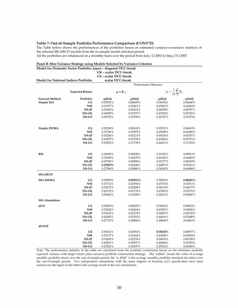
50

Table 7: Out-of-Sample Portfolio Performance Comparison (CONT’D) The Table below shows the performances of the portfolios based on estimated variance-covariance matrices of the selected MGARCH models from the in-sample model selection period. All the portfolios are rebalanced on a monthly basis over the period from July/1/2002 to May/31/2007. Panel B: Min-Variance Strategy using Models Selected by Variance Criterion Model for Domestic Sector Portfolio: Japan – diagonal DCC-break UK – scalar DCC-break US – scalar DCC-break Model for National Indices Portfolio: scalar DCC-break

Performance Measure

Expected Return

t = Rt-1

12

112

1

iitt R

Forecast Method Portfolio μ(Ret) μ(Std) μ(Ret) μ(Std) Simple MA GS 0.30592% 0.00609% 0.30692% 0.06640% NM 0.31557% 0.25061% 0.45021% 0.62418% DS-JP 0.03282% 0.02212% 0.04338% 0.06797% DS-UK 0.43099% 0.01757% 0.43535% 0.05726% DS-US 0.29322% 0.15789% 0.26727% 0.51574%

Simple EWMA GS 0.30594% 0.00610% 0.30701% 0.06610% NM 0.31554% 0.25055% 0.45030% 0.62400% DS-JP 0.03284% 0.02213% 0.04336% 0.06787% DS-UK 0.43097% 0.01755% 0.43546% 0.05721% DS-US 0.29292% 0.15778% 0.26811% 0.51510%

RW GS 0.30609% 0.00838% 0.31921% 0.09013% NM 0.31949% 0.26470% 0.43628% 0.66482% DS-JP 0.03796% 0.02894% 0.03177% 0.08369% DS-UK 0.43203% 0.02446% 0.44871% 0.07631% DS-US 0.27594% 0.20480% 0.26565% 0.66088%

MGARCH MG-EWMA GS 0.30599% 0.00551% 0.30874% 0.06041% NM 0.31712% 0.24784% 0.45735% 0.62011% DS-JP 0.03272% 0.02200% 0.04119% 0.06677% DS-UK 0.43123% 0.01774% 0.43505% 0.05770% DS-US 0.29682% 0.15298% 0.28213% 0.50481%

MG-Simulation df=0 GS 0.30589% 0.00825% 0.58343% 0.08852% NM 0.32242% 0.26264% 0.45051% 0.65436% DS-JP 0.03433% 0.02276% 0.04057% 0.06705% DS-UK 0.43065% 0.02352% 0.44691% 0.07488% DS-US 0.27755% 0.18886% 0.28849% 0.65863%

df=0.05 GS 0.30612% 0.00783% 0.58432% 0.08977% NM 0.32117% 0.26164% 0.44940% 0.65504% DS-JP 0.03426% 0.02276% 0.04054% 0.06708% DS-UK 0.43061% 0.02357% 0.44566% 0.07493% DS-US 0.27821% 0.18537% 0.29212% 0.65681%

Note: The performance statistics in the table are calculated from the portfolio constructed based on the minimize portfolio expected variance with target return (min-variance) portfolio construction strategy. The “(Ret)” means the value of average monthly portfolio return over the out-of-sample period; the “ (Std)” is the average monthly portfolio standard deviation over the out-of-sample period. Two independent simulations with the same degrees of freedom (d.f.) specification have been carried out, the figure in the table is the average result of the two simulations.

51

Table 7: Out-of-Sample Portfolio Performance Comparison (CONT’D) The Table below shows the performances of the portfolios based on estimated variance-covariance matrices of the selected MGARCH models from the in-sample model selection period. All the portfolios are rebalanced on a monthly basis over the period from July/1/2002 to May/31/2007. Panel C: Max-U Strategy using Models Selected by Utility Criterion Model for Domestic Sector Portfolio: Japan – diagonal ADCC UK – diagonal ADCC US – scalar DCC-break Model for National Indices Portfolio: scalar ADCC-break

Performance Measure

Expected Return

t = Rt-1

12

112

1

iitt R

Forecast Method Portfolio μ(U) μ(Ret) μ(Std) μ(U) μ(Ret) μ(Std) Simple MA GS -0.06792 0.92035% 3.38798% -0.05086 0.60760% 2.43832% NM -0.07177 0.87072% 3.58680% -0.06777 0.81524% 3.38185% DS-JP -0.09049 1.16561% 4.42593% -0.07663 0.86009% 3.59237% DS-UK -0.09900 0.57900% 4.68573% -0.08554 0.53547% 4.15653% DS-US -0.09460 0.32598% 4.43001% -0.07808 0.53063% 3.78322%

Simple EWMA GS -0.06674 0.98648% 3.33943% -0.05325 0.36002% 2.43888% NM -0.07159 0.84881% 3.55615% -0.06797 0.79959% 3.38279% DS-JP -0.08835 1.24278% 4.33740% -0.07521 0.91023% 3.54123% DS-UK -0.10035 0.56377% 4.75757% -0.08645 0.48865% 4.17596% DS-US -0.09386 0.32159% 4.42842% -0.08202 0.14313% 3.80194%

RW GS -0.06901 0.69257% 3.28385% -0.05772 0.58287% 2.77087% NM -0.07350 0.82335% 3.63029% -0.06960 0.75568% 3.44122% DS-JP -0.08506 1.26420% 4.10517% -0.07588 0.91175% 3.54935% DS-UK -0.09664 0.62947% 4.60936% -0.09079 0.56856% 4.38960% DS-US -0.09502 0.24755% 4.44654% -0.08192 0.43842% 3.99365%

MGARCH MG-EWMA GS -0.06711 0.90000% 3.36502% -0.04965 0.67369% 2.41762% NM -0.07124 0.83005% 3.54098% -0.06728 0.79457% 3.32776% DS-JP -0.09212 1.13163% 4.49803% -0.07723 0.91756% 3.66023% DS-UK -0.09794 0.57931% 4.64720% -0.08380 0.60178% 4.10626% DS-US -0.09314 0.41850% 4.41177% -0.07936 0.50688% 3.89440%

MG-Simulation df=0 GS -0.07183 0.46881% 3.29508% -0.05917 0.29877% 2.65837% NM -0.07306 0.78297% 3.58784% -0.06881 0.74444% 3.37772% DS-JP -0.08752 1.32746% 4.26223% -0.07694 0.92202% 3.60956% DS-UK -0.09873 0.38320% 4.55455% -0.09142 0.38761% 4.31582% DS-US -0.09764 0.12137% 4.46089% -0.08495 0.15166% 3.94013%

df=0.05 GS -0.07282 0.56329% 3.39918% -0.05650 0.56052% 2.65729% NM -0.07380 0.79670% 3.63529% -0.06902 0.72680% 3.38567% DS-JP -0.08802 1.37297% 4.31542% -0.07882 0.81108% 3.64382% DS-UK -0.10162 0.33021% 4.67853% -0.09163 0.39332% 4.33685% DS-US -0.09714 0.25236% 4.52038% -0.08211 0.46590% 3.96350%

Note: The performance statistics in the table are calculated from the portfolio constructed based on the maximize investor utility (max-U) portfolio construction strategy with 130/30 short-sell constrain. The “(U)” means the value of average monthly portfolio utility over the out-of-sample period; the “ (Ret)” is the average monthly portfolio return over the out-of-sample period; the “ (Std)” is the average monthly portfolio standard deviation over the out-of-sample period. Two independent simulations with the same degrees of freedom (d.f.) specification have been carried out, the figure in the table is the average result of the two simulations.

Figure 1: Pre- and Post-Event Correlation News Impact Surface The structural break point is set on the date of 1st, Jan, 1999. The NISs are obtained from the estimation of diagonal ADCC-break MGARCH model.

UK-Industrial and UK-Financial sectors

US-Industrial and US-Financial sectors.