Taking Account of Housing in Measures of Household Income

Kathleen Short, Amy O’Hara, Scott Susin Housing and Household Economic Statistics Division

U.S. Census Bureau Washington, D.C. 20233

January 2007

Prepared for Session Organized by the Society of Government Economists for the Annual Meeting of the Allied Social Sciences Associations

Chicago, Illinois This report is released to inform interested parties of ongoing research and to encourage discussion of work in progress. The views expressed on statistical, methodological, technical, or operational issues are those of the author and not necessarily those of the U.S. Census Bureau.

Background

In 1977 the United Nations issued provisional guidelines on statistics of the distribution of

income, consumption and accumulation of households. The starting point for the discussion in their report

was the system of national accounts and the extension to the study of the distribution of these flows among

population subgroups. As is done in the national accounts, this group recommended that imputed income

from owner-occupied housing be included in a measure of income for households. On balance, rental

expenditure should also be imputed as an item of household consumption.

In 1987 an international expert group, referred to as the Canberra group, met to advance the

quality of income statistics and to promote international comparability. The primary goal of this group was

to enhance national household income statistics by developing standards on conceptual and practical issues

related to the production of income distribution statistics. They addressed common conceptual, definitional

and practical problems faced by national and international statistical agencies in this important area.

The Canberra group released a report in 2001 that outlined conceptual ground rules for defining

and measuring household income. As part of that conceptual framework their report treats inclusion of

housing-related items in income, the inclusion of the value for housing subsidies and an imputed net rent to

owned homes. The income concept recommended by this group is meant to capture ‘current economic

well-being.’ Sources of income included are employee income, income from self-employment, property

income, and transfer income. The sum of these parts equals total income. Deductions for taxes and social

insurance contributions yield disposable income. Addition of social transfers in-kind yields adjusted

disposable income. This last definition includes both cash and noncash inputs. Resources received in

noncash form include health care, housing, education, childcare, transportation, food, and other subsidies

from governments or other third parties

Following the structure described in the Canberra report, self-employment income includes profit

from unincorporated businesses, sole proprietorships, and royalties. This section also included home

production such as food prepared at home and subsistence agriculture. Also under this heading is imputed

income from owner-occupied dwellings. This is defined as the imputed value of the services provided by a

household’s residence after deduction of expenses such as interest paid on mortgages and property taxes.

2

The Canberra report stated that the purpose of this calculation is to equalize the treatment of

housing between homeowners and renters. As in the system of National Accounts, the approach considers

homeowners as unincorporated enterprises that lease the house back to the household. The value of the

lease is set at the market rent for a similar house and the imputed income is equal to this value less the costs

incurred by the household in their role as landlord (p. 121). These costs include expenses such as

depreciation, property taxes, and interest paid on loans to purchase the owner-occupied dwelling.

Housing subsidies received also fall under the rubric of in-kind or noncash transfers, but were not

a part of total income as defined by the Canberra group1. As such, this paper will focus on net imputed

rental income in an income measure and treat valuing housing subsidies elsewhere. The final section of the

Canberra report lists this among the areas that are most fruitful to pursue (p. 62). The report stated that this

area, the treatment of housing, is important because homeownership rates vary widely among countries,

and is essential for making comparisons of economic wellbeing across countries.

As noted in their report, a chief problem in including housing in income is the accurate

measurement of imputed rent. Estimates of the gross rental value as well as taxes, depreciation, repair and

upkeep, interest charges, property taxes and other shelter costs, are required. (See Eurostat, 1998 and 2000a

for their approach). One approach is to estimate a return on the equity in owned home (Smeeding et al.,

1993). Given information about equity in an owned home this method requires careful selection of an

appropriate rate of return. The report further notes that if this method is followed, care should be used to

measure this in a way that is not nation specific. Unreasonably high land values, such as for Tokyo, Hong

Kong, or New York, would distort the values for residents there. This method can lead to unreasonably

high values of net imputed rent. Johnson and Smeeding (2000) note that low income elderly homeowners

may spend 30 to 40 percent of their incomes on shelter costs, which are not explicitly accounted for in

these types of measures. This suggests that methods based on reported market value of owned home may

be less desirable than those based on rental markets.

Finally, the report notes that estimates are imputed at the macro level by most countries for their

national accounts. They encourage micro-data users to investigate the methodology and data sources used

to make macro-level estimates with a view to drawing on them in producing micro-level estimates (p.64).

1 Value of housing subsidies are included in the Canberra definition of Adjusted Disposable Income.

3

In 2003, the Bureau of Economic Analysis calculated Rental Income of persons with Capital Consumption

Adjustment to be $79 billion.

Following the release of the Canberra Group report, the International Labor Organization released

a report on household income and expenditure statistics. They revised an earlier report to also present new

international guidelines for the production of income and expenditures statistics. Under the heading of

income from household production of services, this group also listed services of owner-occupied housing as

an addition to income.

In general, the studies and reports state that the purpose of this calculation is to extend the

examination of income distributions as measures of economic wellbeing. The calculation of income

distributions that include a faithful representation of access to resources is important in understanding

inequality of such resources among the population. Following treatment in the national accounts,

comparisons of economic well-being appropriately equalize the treatment of homeowners and renters. This

is especially important for international comparisons as the rate of ownership is a matter of custom, culture,

and institutions, and varies widely across countries.

In addition to comparing income distributions, another goal of policymakers is to understand and

measure the incidence of poverty, or the inability of segments of the population to meet basic needs. One

must ask the following question “Does this definition of income make sense in a measure of poverty?”

Clearly, the measure of resources used to estimate poverty rates must be compared to a consistently drawn

poverty line (see Citro and Michael 1995). At this point it is sufficient to note that generally this definition

of income will have to be adjusted to measure poverty. One important example concerns whether the

poverty line is not different by geographic area, as is the current U.S. official poverty line. In this case,

valuing housing by geographic area results in misclassification of the incidence of poverty. If the threshold

does not represent differences in housing costs across geographic areas, then the notion that net imputed

rent or return to home equity is part of resources is problematic. Housing values and costs vary greatly by

area. There are differences in rent-to-value ratios for low and high cost housings markets, suggesting one

might add a single conservative national number to income for this purpose. There is a difference in

treatment of housing for income distribution and for poverty measures: for income it is important to

4

consider the distribution across the entire population, and to reproduce the distributions of imputed net rent

to all homeowners including variation across geographic area.

The Value of Owner-Occupied Housing Services

The goal is to compute after-tax net implicit income from owner-occupied housing, defined as:

(1) Rn = (Rg – I - C) + pV where

Rn = after tax net implicit rental income Rg = implicit gross rent I = Mortgage interest expense

C = operating costs such as maintenance and depreciation, net of tax preferences p = expected appreciation rate of owner-occupied housing V = house market value Many approaches to calculating implicit rental income are based on the assumption that rents (Rg) are

determined by the “user cost” (for example, see Poterba 1984).

(2) Rg = (r + c - p)V

where

r = rate of return on rental housing (mortgage rates plus a risk premium).

c = operating costs as a proportion of house value

Substituting (2) into (1) gives: Rn = (rV – I ) = rV – iM, where i is the nominal mortgage interest rate and M is the mortgage balance remaining to be paid. If we assume that rate of return on rental housing equals the mortgage rate, the equation simplifies to (3) Rn = i(V –M). Valuation Methods

There are several approaches taken in the literature to value imputed rents. We list them here as

Method 1.) return to equity approach ( Smeeding et al., 1993 ), Methods 2 and 3.) a capitalization rate

approach (Yates 1994, Crone et al., 2004), and Method 4.) a rent hedonic approach ( Frick and Grabka,

2003). In the following, we examine these different valuation methods using the 1997-2003 American

Housing Survey data and compare and contrast the results from each approach.

5

Method 1. Return to equity approach

The Census Bureau has included an approximation to implicit net rent in its alternative income

series for several years, as in Smeeding et al. 1993. The calculation uses a combination of Current

Population Survey (CPS-ASEC) and American Housing Survey (AHS) data to estimate home equity for

each household.2 Then equation (3) is applied, taking i as the current year’s return to municipal bonds.3

It should be clear that the implicit rent calculated in this manner will be very sensitive to the rate

of return on rental housing (r) chosen. The Census Bureau uses a return to municipal bonds as a stable and

conservative rate of return. Others have used mortgage interest rates, the rate on short-term bonds (Poterba

1984), or mortgage rates plus a risk premium. Hence, implicit rent calculated using the return to equity

approach will necessarily be somewhat arbitrary, which is a drawback to this method.

Methods 2 and 3. Capitalization rate approach

Several authors have suggested estimating a = Rg/V, the capitalization rate, and then applying this

to equation (1), yielding

(4) Rn = (a + p) V – I – C

(Yates 1994, Crone, Nakamura, and Voith 2004). These methods calculate a rent-to-value ratio

from various sources to transform value of owned home into a market rent. Yates used the rent-to-value

ratios implicit in the national product accounts for Australia to derive imputed rent and microdata to

subtract associated costs. Crone et al. used hedonic techniques to estimate a capitalization rate that makes

the marginal consumer indifferent between renting and owning. They estimated:

ln ( V or Rg) = a D + bX + e

where V = value of home, if owner Rg = gross rent, if renter D = dummy variable, 1 if owner occupied, 0 otherwise X = vector of housing amenities

Estimating this equation for a pooled sample of owners and renters, yields the capitalization rate A

= exp(-a), which, when multiplied by market value of home represents the stream of housing services to a

2 Home equity is not collected on the CPS, so a statistical match, based on household characteristics that include geography and income, obtains this information from the AHS. 3 In practice, property taxes are then subtracted from calculated return to home equity.

6

given homeowner. Since the dependent variable is the log of observed gross rents (or house values), A

represents a gross capitalization rate. Property taxes, maintenance costs, and other expenses must be

subtracted from the gross rent, as indicated in equation (4).

This approach eliminates the need to choose a rate of return, but it adds a difficulty of its

own, including p, the house price appreciation rate, in order to calculate the annual unrealized capital gains

of homeownership (pV). We discuss this issue further below. For now, note that unless unrealized capital

gains from homeownership are included in the capitalization rate estimates, this measure of implicit rent is

not conceptually equivalent to the home equity approach.

One shortcoming of the Yates approach is that it only yields one capitalization rate for the whole

U. S. whereas the Crone, Nakamura, Voith approach can be enhanced to vary geographically by housing

cost. This is discussed further in the results section.

Method 4. Hedonic approach

Another way of directly using equation (1) Rn = (Rg – I - C) + pV, is by estimating gross rent with

a hedonic regression (Frick and Grabka, 2004). That is, the hedonic equation

ln (Rg) = bX + e

is estimated in a sample of renters and the model is then used to predict a market rent for homeowners in

similar types of homes. Once predicted rents are available for homeowners, operating costs may be

subtracted to arrive at the net imputed rent that we require following Yates (1994).

This approach is quite similar to the capitalization rate approach. In fact, if the assumptions of the

capitalization rate model are met, these two methods will yield identical results. The capitalization rate

model imposes the assumption that the regression coefficients for renters and owners are the same by

estimating a single set of coefficients for both groups, allowing only the constant to differ across tenure

types. One important difference is that the capitalization rate approaches, as described above, assign a

single rate across all geographic areas, while it is apparent that rent-to-value ratios vary considerably from

place to place. This approach incorporates geographic difference in the predicted value by using Fair

Market Rents by county combined into deciles. Dummy variables for deciles are referred to as FMR

indicators.

7

House Price Appreciation

As with interest rates, a variety of possible measures of p could be used, such as the Freddie

Mac/OFHEO repeat sales index, or the Census Bureau price index of new single-family homes. In

addition, house price appreciation obviously varies considerably across the country, so we would ideally

want a large set of indexes. This problem did not arise for Crone et al, since they were interested in

measuring inflation in the cost of housing services, rather than imputed rents as such. The choice of p also

does not arise either for Yates, because her definition of net rental income excludes unrealized house price

appreciation. Yates was interested in generating an estimate of implicit rental income consistent with

national accounts, which do not include unrealized capital gains, so her choice of definition was clear. In

the U.S. rental income of persons in the U.S. National Income and Product Acccounts (NIPA), like other

measure of income included there, excludes capital gains or losses resulting from changes in the prices of

existing assets (see Mayerhauser and Reinsdorf, 2005).

Data and Results

The American Housing Survey (AHS) is a household survey that asks questions about the quality

of housing in the United States. In gathering information, the Census Bureau interviewers visit or telephone

the household occupying each housing unit in the sample. For unoccupied units, they obtain information

from landlords, rental agents, or neighbors. The AHS is actually two surveys. The AHS conducts a national

survey and a metropolitan area survey. Both surveys are conducted during a 3- to 7- month period. This

study only uses the national survey.

The national survey, which gathers information on housing throughout the country, interviews at

about 55,000 housing units every 2 years, in odd-numbered years. A sample of housing units in all survey

areas was selected from the decennial census. These are updated by a sample of addresses obtained from

building permits (for new construction) to include housing units added since the sample was selected. The

survey goes back to the same housing units on a regular basis, recording changes in characteristics, adding

and deleting units when applicable.

8

The Census Bureau has interviewed the current sample of housing units since 1985. The AHS

sample is comprised of these units from the sampled PSUs:

• Housing units selected from the 1980 census

• New construction in areas requiring building permits

• Housing units missed in the 1980 census

• Other housing units added since the 1980 census

The AHS for 2003 sampled all occupied units in the U.S. The size of the sample was about 47,000

housing units. Of , about 69% were owner occupied units. The exercise described below only included

housing units owned or rented for cash. We also excluded outliers. If rent paid was reported to be less than

$10 or the value of the home was greater than $1,000,000 they were excluded from the analysis. We

attached 2-bedroom FMRs for counties to each unit and categorized them by deciles in order to account for

variation in housing prices by geographic area.

For method one, we calculated home equity for all homeowners and applied the rate used by the

Census Bureau. For 2003 this rate of interest was 4.73 percent. From this value we subtracted property

taxes in order to replicate the method in Census Bureau’s alternative income calculations. This method

gives an aggregate dollar amount for imputed net rents of $235 billion for all homeowners in the U.S.

The second method follows Yates and used figures from the national accounts to calculate a rent-

to-value ratio. In the U.S. the NIPA method for the PCE accounts uses data from the Residential Finance

Survey (RFS) and the American Housing Survey to value imputed rents. Space rents paid for owned

property are used to create ratios for rent to reported market values from the RFS. Using only one-unit

properties for this purpose, these ratios were applied to categories of market values for households in the

AHS. This figure was updated with the CPI for owners’ equivalent rent between collections of the

decennial RFS and for 2003 this was 6.78 percent.

Reported operating costs for each housing unit in the AHS were subtracted from rent, following

Yates. These costs included routine maintenance expenses, mortgage interest expense and insurance,

property taxes paid, and a depreciation expense. We assumed depreciation of 1 percent per year of house

value. Figure 1 shows the gross rent and operating expenses from the NIPA accounts compared to those

9

based on this method. The aggregate costs reported in the AHS are lower than those subtracted in the

NIPA except for property taxes. Therefore, while the gross rent figures from this method closely replicate

the NIPA figures, the resulting aggregate value of net rental income from the BEA calculations for 2003,

$79 billion, is much below the aggregate value from this method of $212 billion.

For the third method we followed Crone et al. (2004) to estimate a capitalization rate for 2003.

This method included renters and owners together in a hedonic regression to capture the parameter that

translates the value of home into a market rent. Following their specification we calculated a capitalization

rate for owned home of 8.14 percent for 2003. This compares favorably with Crone et al., who estimated a

range of capitalization rates from 8.1 to 9.0 percent over the period from 1985 to 1999. In addition, we

estimated a more comprehensive model, including all of the characteristics as in the hedonic regression

described below for method four. This fuller model gave a lower capitalization rate of 7.23 percent. For

homeowners, we then multiplied the value of the home by the capitalization rate to yield implicit rent.

Subtracting monthly costs gave us the income from home ownership. Monthly costs subtracted include

maintenance costs, mortgage interest cost, property taxes and depreciation, as in method two. The

aggregate figure for net imputed rent for all homeowners from this method was $270 billion.

One advantage of this method over the Yates method, however, is that it allows us to estimate a

different capitalization rate for different areas. We do this by including interaction terms with the tenure

dummy variable and the FMR dummy variables that capture housing price variation. This allows us to

calculate a different cap rate for each of the 10 FMR decile areas. Results from this variation are an

aggregate figure of $250 billion in 2003. The estimated rates are lower and the estimated net rental income

is below the single rate method, though still above the Yates approach. Table 1 shows the summary

statistics and regression results from this estimation.

The final method is an estimated hedonic regression predicting market rent using only renters in

the AHS. Housing characteristics are included in the model along with the FMR decile dummies. Results

from this regression are shown in Table 2. We used this model to predict rents for homeowners given the

housing characteristics and location. After correcting for the log transformation, this model yielded an

imputed rental value from which we subtracted, as above, monthly housing costs. The remaining amount is

10

the income this homeowner would receive, clear of expenses, from renting his or her owned home. The

aggregate value of this rental income is much lower than other methods, $38 billion for 2003.

At this point, tax expenses only include payment of property taxes and as such do not take account

of the income tax benefits of home ownership. Noting that these are significant, they will be addressed in

the next step when rental income is attached to the incomes of households in the CPS and the after-tax

income is calculated. In 2003, individual income tax filers reported $325 billion4 of home mortgage interest

to the IRS when itemizing their deductions. This comprised more than one-third of the total itemized

deductions claimed that year. For AHS 2003, the aggregate amount of total interest paid was $291 billion.

Interest paid and real estate taxes paid are allowable expenses when itemizing deductions. The

deductibility of these expenses will be addressed in future work, when imputed rental income is attached to

the incomes of households in the CPS. At that point, marginal federal and state income tax rates will be

determined according to CPS reported income and applied to the allowable housing expenses to compute

the individual income tax benefit. Preliminary calculations suggest that 17.1 million households would

receive a reduction of about $27 billion dollars in tax liabilities from the tax advantages from

homeownership. This would add roughly $856 to the median estimates of imputed rental income calculated

in this paper.

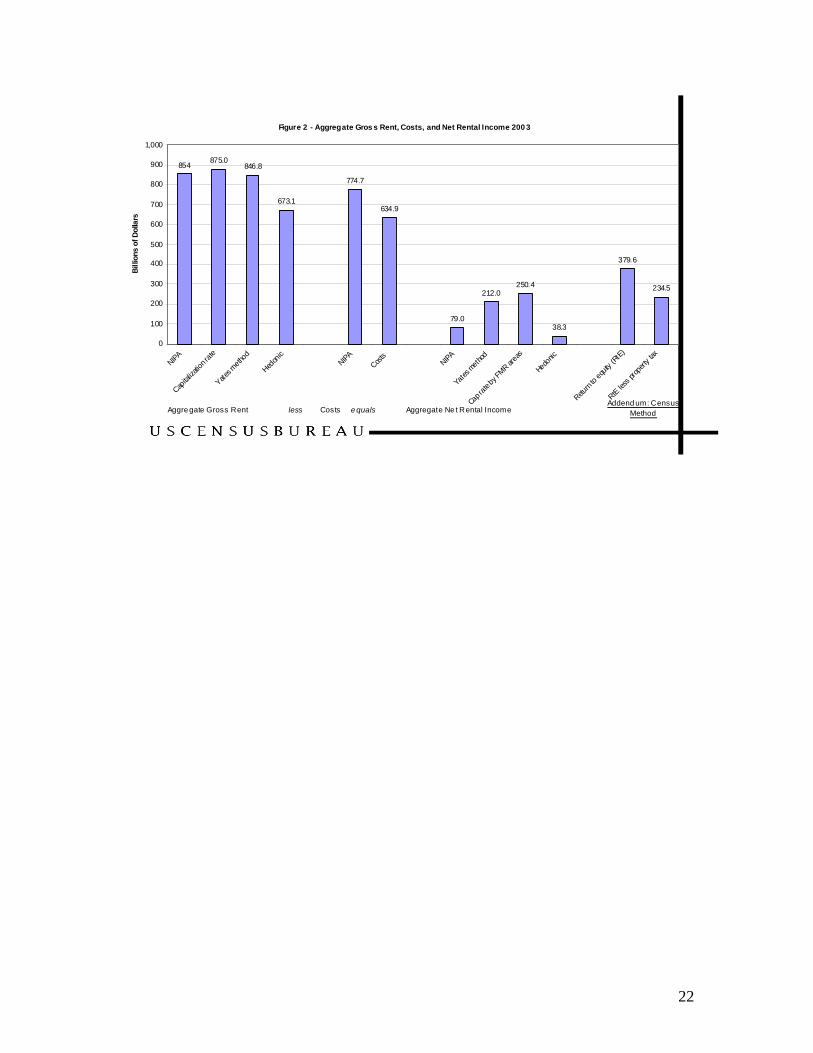
The several methods used here to value imputed net rent yield widely different results as shown in

Figure 2. The first bar represents the aggregate value for space rent in the NIPA. The next three bars are

aggregate values as estimated using methods 2, 3 and 4. The fifth bar is aggregate costs, which are

subtracted from imputed rents at the household level. The second group of bars is imputed rental income of

persons in 2003 net of expenses. This is the set of figures that represents the concept of interest to us,

beginning with rental income of persons as measured by BEA, $79 billion in 2003. All of our valuation

methods yield a much larger aggregate figure, except for the hedonic method, which is much lower.

Distribution of net rental income

The next set of charts shows estimates of net imputed rent using the four methods for 20

categories of households arranged by income and age of householder. This illustrates the distributional

4 IRS SOI Bulletin vol 25 no 3 winter 2005-6.

11

impact of the various valuation methods for important groups. The first 10 groups are householders under

the age of 65 by income decile. The second 10 categories are income deciles of elderly households.

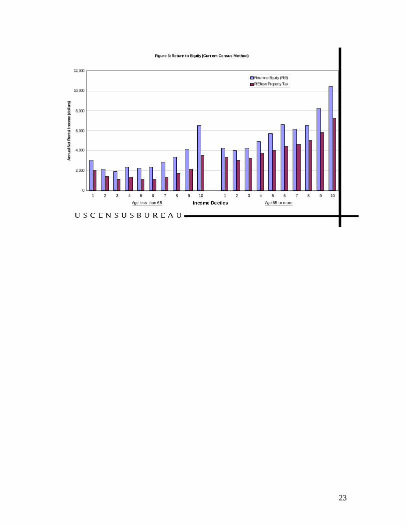
Figure 3 compares return to home equity with and without subtracting property taxes. As shown

above, this method should incorporate costs in the chosen rate of interest and no subsequent subtraction

should be done. Subtracting property taxes has an effect that appears to be proportional to income, possibly

reflecting the correlation between incomes and property values by geographic area. This has the effect of

lowering overall net imputed rent added by the Census Bureau for higher income households relative to

lower income households.

Figure 4 and Figure 5 compare return to home equity (without subtracting property taxes) to the

two capitalization rate methods. These methods are very similar, multiplying reported market value of

home by a percentage and subtracting costs. The main difference between the two is that the Yates method

yielded a lower capitalization rate than the Crone et al. method and the Crone et al. method shown here

incorporates geographic differences in FMRs across areas. Comparing the two distributions suggests that

accounting for varying capitalization rates yields higher rental income overall.

One observation from this comparison is that the return to home equity method is similar to the

other methods for older households, but overestimates net imputed rent for younger households. This

reflects the fact that younger households have very large mortgage interest costs compared with older

households. It suggests further that the Census method, that subtracts property taxes only from return to

home equity, overestimates net imputed rent for younger households, but underestimates this for older

households because it takes no account of other operating costs that vary across the life cycle.

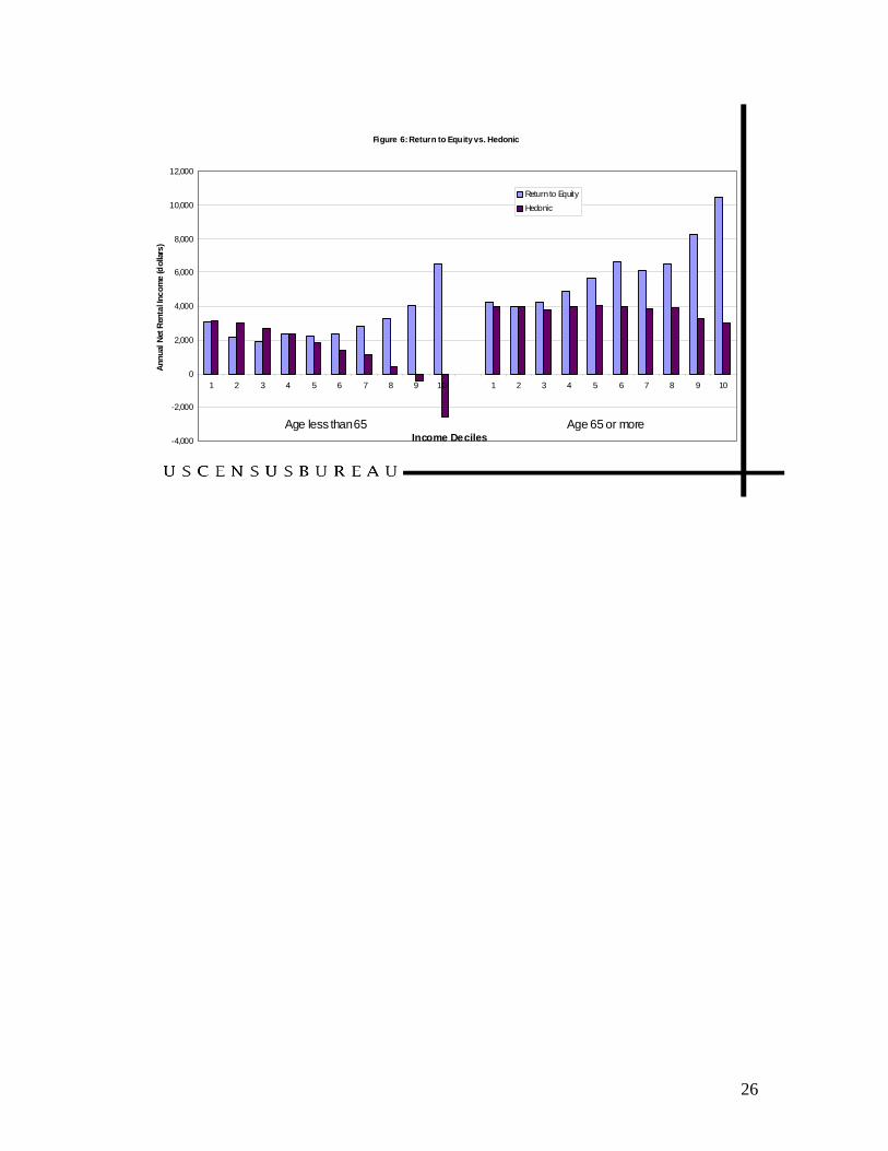
Finally, the distribution of net imputed rent using the hedonic method is shown in Figure 6 with

return to home equity. Here we see a much different pattern than the other methods. For young households

there is a negative relationship with income, actually becoming negative for the highest income deciles of

young households. For the elderly, there is no discernible relationship with income. For this group median

net imputed rent is about $4,000 to $5,000 regardless of income, suggesting that rents may be under-

predicted for higher value homes by this method.

Clearly, all methods show much larger flows from owned homes for elderly households than for

younger households. In general, this results from the lower operating costs elderly householders face due to

12

having paid off mortgages. This illustrates one main problem with the return to equity approach in that it

cannot account for differential costs between specific population subgroups. Among the other methods, the

largest amounts come from the capitalization rate method. The smallest amounts are from the hedonic

approach that also has a different relationship with income deciles than the methods based on market value

of owned home.

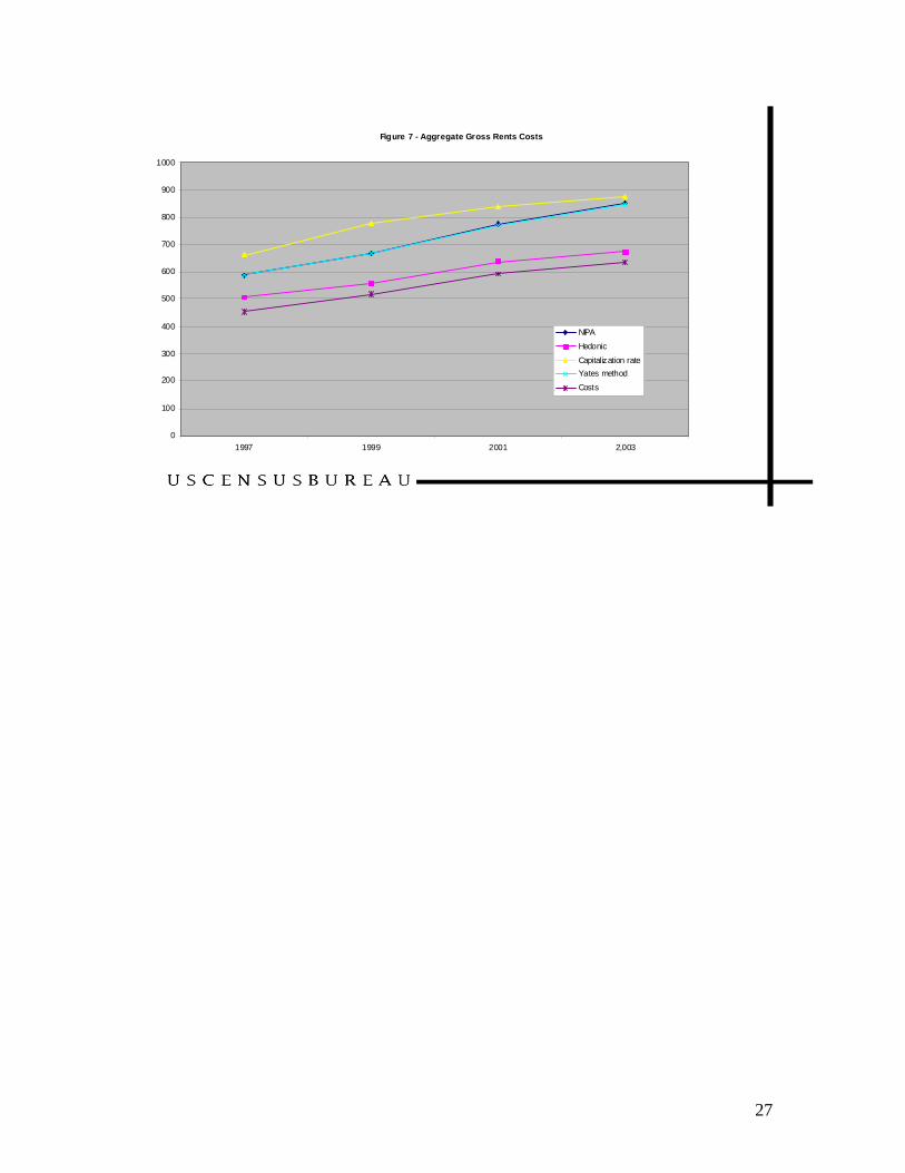
Net Rental Income over time

Using the 1997, 1999, 2001, and 2003 AHS we calculated the different methods to see how they

behave over time. Figure 7 charts our estimates of aggregate rent before costs are subtracted compared

with those of BEA. The chart also plots aggregate costs across owner occupied households in the AHS. The

rents based on BEA rent-to-value ratios are nearly identical to the NIPA rents. All methods show increasing

rents over the period from 1997 to 2003 with slightly different rates of increase year-to-year.

Figure 8 shows net rental income after operating costs have been subtracted from rent at the

household level over the same period. There is a wide variation in trends, as well as levels, over the period.

In general, two methods follow an upward trend across the period – the return to equity approach and the

method following Yates. These two methods are least able to match rents to housing costs by area. Two

methods rise and then fall, rental income from NIPA and the cap rate approach. The hedonic method varies

across the period ending lower in 2003 than in 1997. Overall, across the four years of AHS data examined

here, median home values rose slightly along with median rents from 1997 to 1999, but from 1999 to 2003,

home values rose much faster than median rents, 20 percent compared with 9 percent. This might suggest a

steady and then falling rent-to-value ratio across the period and favor the methods with a downward trend,

given that costs, while varying over the period, are measured similarly across the methods.

Next steps

Overall, this paper describes several approaches to calculating imputed net rental income for

owner-occupiers for an income measure. This effort follows recommendations of the Canberra and ILO

reports on improving income measures and examines the current Census Bureau method. One other

approach in the literature, not tested here, evens the treatment of owners and renters by subtracting housing

13

costs from income rather than adding imputed rents (Ritakallio 2003, Siminksi and Saunders 2004).

Siminski and Saunders argue that including imputed rental income is preferable to cash income for

distributional analysis across housing tenure or life cycle differences, but does nothing to address the

problem of regional housing price differences. Subtracting housings costs from income is a way to take

geographic differences into account. This is a method we will investigate in future work.

For now, once we have selected the best method of computing net rental income, the next step is

to attach these computations to the CPS or SIPP, in order to make the remaining tax and transfer

calculations. Future work will investigate how to conduct a statistical match to other surveys that contain

limited information about housing characteristics. In the CPS, for example, all we have is housing tenure,

so a statistical match must be based on household characteristics, including geography, that are common to

both surveys.

The resulting income measures may be used for calculating poverty statistics, if a relative measure

is employed, ensuring that the threshold (some percentage of median equivalised income) is consistently

measured. If some other poverty threshold is employed, other considerations are required to make sure the

accounting for housing needs are consistently calculated. Garner (2005) points out that rental income for

homeowners is added to income to help meet housing consumption needs that should be a part of the

poverty threshold calculations. As an example, if housing costs do not vary by geographic area in the

thresholds, then adding imputed rents that are higher in the northeast, for example, and lower in the south,

contributes to misclassification by poverty status. Future work will address these issues.

Finally, the issue of valuing housing subsidies is another important housing issue not addressed in

this paper. Obviously, this will involve some similar calculations and concepts as we have developed in this

paper, but for now remains in the area of future work.

Conclusion

This paper has presented work to evaluate net imputed rental income of homeowners to be included in a

measure of income for the purpose of examining distributions of economic well-being. The paper describes

several approaches and compares these to calculations currently used by the Census Bureau and to those in

14

the NIPA by BEA. We believe that we have found some acceptable methods, although, each method has

some problems. Our next step is to choose one and go forward with including that in measures of income.

The questions that are important in the selection of the best method include questions about levels.

What is the size of net rental income to homeowners? Is the amount in the NIPA the right target in terms of

size? If so, how do we improve the costs that are subtracted from imputed rent to arrive at the ‘correct’

amount? For international comparisons it is important that aggregate levels are similarly calculated. For

inter-household comparisons, levels are less important, as long as the relative standing between renters and

homeowner in a distribution of economic wellbeing is addressed. These issues, along with more practical

concerns will be considered in future work.

15

References

Blackley, Dixie M. and James R. Follain. In Search of the Linkage between User Cost. and Rent. Regional Science and Urban Economics, 26, 1996, pp. 409-31 Citro, Constance F. and R.T. Michael, eds., Measuring Poverty : A New Approach. Washington, DC: National Academy Press, 1995. Crone, Theodore, Leonard I. Nakamura, and Richard P. Voith, “Hedonic Estimates of the cost of housing services: rental and owner-occupied units,” Federal Reserve Bank of Philadelphia, Working Paper #04-22, October, 2004. Frick, Joachim and Markus M. Grabka, “Imputed rent and income inequality: a decomposition analysis for Great Britain, West Germany and the U. S.,” Review of Income and Wealth, 49(4), pp.513 – 538, December, 2003. Garner, Thesia I. and Patricia Rozaklis, “Owner-Occupied Housing: An Input for Experimental Poverty Thresholds,” SGE-ASSA Annual Meeting, New Orleans, Louisiana, January 6, 2001, Poverty Measurement Working Paper, Census Bureau web site. Garner,Thesia I., and Kathleen S. Short, Owner-Occupied Shelter in Experimental Poverty Measures November 15, 2001, Poverty Measurment Working Paper, http://www.census.gov/hhes/www/povmeas/topicpg5.html Garner, Thesia, “Incorporating the Value of Owner-Occupied Housing in Poverty Measurement,” unpublished paper prepared for the National Academy of Sciences Workshop on Experimental Poverty Measures, Washington, D.C., June 2004 International Labour Office, Report II: Household income and expenditure statistics, Seventeenth International Conference of Labour Statisticians, Geneva, 24 November- 3 December 2003. Johnson, David, Stephanie Shipp, and Thesia I. Garner, “Developing Poverty Thresholds Using Expenditure Data,” in Proceedings of the Government and Social Statistics Section, Alexandria, VA: American Statistical Association, August 1997, pp. 28-37. Malpezzi, Stephen, Gregory H. Chun, and Richard K. Green, “ New place to place housing price indexes for us metropolitan areas, and their determinants,” Real estate economics, 26(2) 1999, pp 235-274. Mayerhauser, Nicole and Marshall Reinsdorf, “Housing Services in the National Economic Accounts,” 2005, www.BEA.gov. Phillips, Robyn S., “Residential Capitalization Rates: Explaining Intermetropolitan Variation, 1974-1979,” Journal of Urban Economics 23, 278-290, 1988. Poterba, James, “Tax Subsidies to Owner-Occupied Housing: An Asset-Market Approach,” The Quarterly Journal of Economics, 99(4), November, 1084, pp. 729-752. Ritakallio, V.M., “The Importance of Housing Costs in Cross-National Comparisons of Welfare Outcomes,” International Social Security Review, 56(2), 2003, pp. 81-101. Saunders, Peter and Peter Siminski, “Home ownership and inequality: imputed rent and income distributionin australia’, Forthcoming. Siminski, Peter and Peter Saunders, “Accounting for Housing Costs in Regional Income Comparisons,” Australasian Journal of Regional Studies, 10(2), 2004.

16

Smeeding, T., P. Saunders, J. Coder, S. Jenkins, J. Fritzell, A.J.M. Haganaars, R. Hauser, and M. Wolfson, “Poverty , Inequality, and Family Living Standards Impacts across Seven Nations: The Effect of Non-cash Subsidies for Health, Educaiton, and Housing,” The Review of Income and Wealth, 39(3), 229-56, 1993. U. S. Census Bureau, Measuring the Effect of Benefits and Taxes on Income and Poverty: 1979 to 1991, P60-182-RD, 1992. Verbrugge, Randal (2005) “The puzzling divergence of rents and user costs, 1980-2004” Mimeo, Bureau of

Labor Statistics. Yates, Judith, “Imputed rent and income distribution,” Review of Income and Wealth, 40(1), March 1994,

pp. 43-66. Yezer, Anthony, “Issues of Return to Home Equity and Rental Equivalence: Implications for Poverty Measurement,” notes, George Washington University, Washington, DC, November 6, 2002.

17

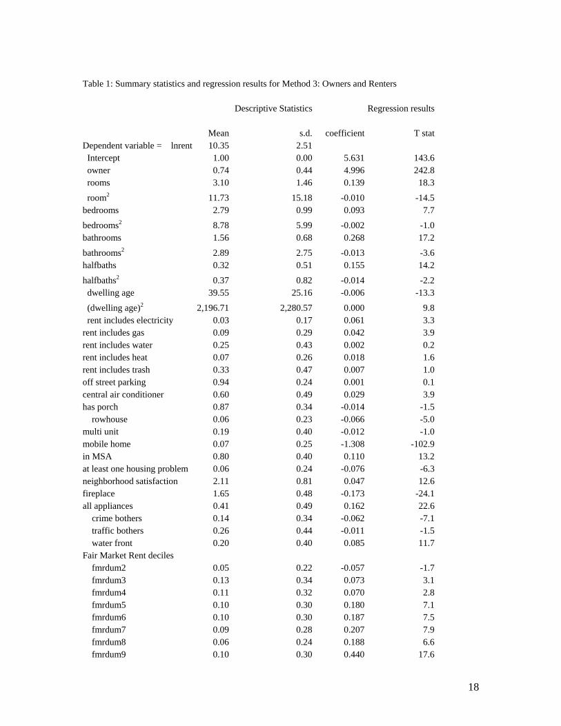
Table 1: Summary statistics and regression results for Method 3: Owners and Renters Descriptive Statistics Regression results Mean s.d. coefficient T stat Dependent variable = lnrent 10.35 2.51 Intercept 1.00 0.00 5.631 143.6 owner 0.74 0.44 4.996 242.8 rooms 3.10 1.46 0.139 18.3

room2 11.73 15.18 -0.010 -14.5 bedrooms 2.79 0.99 0.093 7.7

bedrooms2 8.78 5.99 -0.002 -1.0 bathrooms 1.56 0.68 0.268 17.2

bathrooms2 2.89 2.75 -0.013 -3.6 halfbaths 0.32 0.51 0.155 14.2

halfbaths2 0.37 0.82 -0.014 -2.2 dwelling age 39.55 25.16 -0.006 -13.3

(dwelling age)2 2,196.71 2,280.57 0.000 9.8 rent includes electricity 0.03 0.17 0.061 3.3 rent includes gas 0.09 0.29 0.042 3.9 rent includes water 0.25 0.43 0.002 0.2 rent includes heat 0.07 0.26 0.018 1.6 rent includes trash 0.33 0.47 0.007 1.0 off street parking 0.94 0.24 0.001 0.1 central air conditioner 0.60 0.49 0.029 3.9 has porch 0.87 0.34 -0.014 -1.5 rowhouse 0.06 0.23 -0.066 -5.0 multi unit 0.19 0.40 -0.012 -1.0 mobile home 0.07 0.25 -1.308 -102.9 in MSA 0.80 0.40 0.110 13.2 at least one housing problem 0.06 0.24 -0.076 -6.3 neighborhood satisfaction 2.11 0.81 0.047 12.6 fireplace 1.65 0.48 -0.173 -24.1 all appliances 0.41 0.49 0.162 22.6 crime bothers 0.14 0.34 -0.062 -7.1 traffic bothers 0.26 0.44 -0.011 -1.5 water front 0.20 0.40 0.085 11.7 Fair Market Rent deciles fmrdum2 0.05 0.22 -0.057 -1.7 fmrdum3 0.13 0.34 0.073 3.1 fmrdum4 0.11 0.32 0.070 2.8 fmrdum5 0.10 0.30 0.180 7.1 fmrdum6 0.10 0.30 0.187 7.5 fmrdum7 0.09 0.28 0.207 7.9 fmrdum8 0.06 0.24 0.188 6.6 fmrdum9 0.10 0.30 0.440 17.6

18

fmrdum10 0.14 0.34 0.469 21.0 FMR deciles * owner fmrown2 0.04 0.20 0.023 0.6 fmrown3 0.10 0.30 -0.034 -1.3 fmrown4 0.09 0.29 0.047 1.6 fmrown5 0.08 0.27 0.083 2.9 fmrown6 0.08 0.27 0.043 1.5 fmrown7 0.07 0.25 0.112 3.8 fmrown8 0.04 0.21 0.022 0.7 fmrown9 0.07 0.25 0.276 9.8 fmrown10 0.09 0.29 0.389 15.1

N 43,450 R2 0.9443 Table 2: Summary statistics and regression results for Method 4: Renters Descriptive Statistics Regression results Mean s.d. coefficient T statDependent variable = lnrent 6.35 0.57 Intercept 1.00 0.00 5.495 95.0 rooms 2.40 0.86 0.070 4.8

room2 6.49 7.82 -0.005 -3.6bedrooms 1.98 0.89 0.111 6.1

bedrooms2 4.72 4.08 -0.005 -1.4bathrooms 1.21 0.46 0.242 9.8

bathrooms2 1.67 1.76 -0.027 -4.6halfbaths 0.14 0.38 0.063 3.7

halfbaths2 0.16 0.89 -0.019 -2.9 dwelling age 44.20 25.08 -0.005 -6.0

(dwelling age)2 2,582.52 2,425.37 0.000 3.8 rent includes electricity 0.10 0.30 0.019 1.1rent includes gas 0.18 0.38 0.073 5.6rent includes water 0.64 0.48 0.008 0.7rent includes heat 0.13 0.34 0.046 3.2rent includes trash 0.63 0.48 0.047 4.4off street parking 0.86 0.34 -0.017 -1.2central air conditioner 0.45 0.50 0.051 4.3has porch 0.73 0.44 -0.006 -0.5 rowhouse 0.08 0.27 0.057 2.9multi unit 0.62 0.48 0.047 3.4mobile home 0.04 0.20 -0.324 -12.9in MSA 0.86 0.35 0.172 11.3at least one housing problem 0.10 0.30 -0.035 -2.3neighborhood satisfaction 2.30 0.79 0.037 6.2fireplace 1.87 0.33 -0.094 -6.3

19

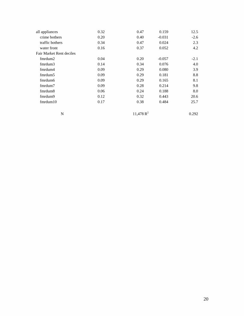
all appliances 0.32 0.47 0.159 12.5 crime bothers 0.20 0.40 -0.031 -2.6 traffic bothers 0.34 0.47 0.024 2.3 water front 0.16 0.37 0.052 4.2Fair Market Rent deciles fmrdum2 0.04 0.20 -0.057 -2.1 fmrdum3 0.14 0.34 0.076 4.0 fmrdum4 0.09 0.29 0.080 3.9 fmrdum5 0.09 0.29 0.181 8.8 fmrdum6 0.09 0.29 0.165 8.1 fmrdum7 0.09 0.28 0.214 9.8 fmrdum8 0.06 0.24 0.188 8.0 fmrdum9 0.12 0.32 0.443 20.6 fmrdum10 0.17 0.38 0.484 25.7

N 11,478 R2 0.292

20

2

Figure 1: Aggregate gross re nt, ope rating e xpe nse s, and ne t re ntal income 2003 NIPA vs. AHS

854

168

123

336

145

79

847

36

145

275

125

212

0

1 00

2 00

3 00

4 00

5 00

6 00

7 00

8 00

9 00

Gros s R ent Maintenance Taxes Interes t D eprec iation Net Rental Inc om e

Bill

ions

of D

olla

rs

NIP A

AHS Method 2

les s equals

21

3

Figure 2 - Aggregate Gros s Rent, Costs, and Net Rental Income 200 3

854875.0

846.8

673.1

774.7

634.9

79.0

212.0250.4

38.3

379.6

234.5

0

100

200

300

400

500

600

700

800

900

1,000

NIPA

Capital

izatio

n rate

Yates m

ethod

Hedon

icNIPA

Costs

NIPA

Yates

method

Cap r

ate by

FMR ar

eas

Hedo

nic

Return

to eq

uity (R

tE)

RtE less p

ropert

y tax

Billi

ons

of D

olla

rs

Aggre gate Gross Rent less Costs e quals Aggregate Ne t Rental IncomeAddend um: Census

Method

22

4

Figure 3: Return to Equity (Current Census Method)

0

2,000

4,000

6,000

8,000

10,000

12,000

1 2 3 4 5 6 7 8 9 10 1 2 3 4 5 6 7 8 9 10

Income Deciles

Annu

al N

et R

enta

l Inc

ome

(dol

lars

)

Return to Equity (RtE)RtE less Property Tax

Age less than 65 Age 65 or more

23

5

Figure 4: Return to Equity vs. Yates

0

2,000

4,000

6,000

8,000

10,000

12,000

1 2 3 4 5 6 7 8 9 10 1 2 3 4 5 6 7 8 9 10

Income Deciles

Ann

ual

Net

Ren

tal I

nco

me

(dol

lar

Return to EquityYates

Age less than 65 Age 65 or more

24

6

Figure 5: Return to Equity vs. Capitalization Rate

0

2,000

4,000

6,000

8,000

10,000

12,000

1 2 3 4 5 6 7 8 9 10 1 2 3 4 5 6 7 8 9 10

Income Deciles

Ann

ual N

et R

enta

l In

com

e (d

olla

r

Return to EquityCapitalization Rate

Age less than 65 Age 65 or more

25

7

Figure 6: Return to Equity vs. Hedonic

-4,000

-2,000

0

2,000

4,000

6,000

8,000

10,000

12,000

1 2 3 4 5 6 7 8 9 10 1 2 3 4 5 6 7 8 9 10

Income Deciles

Annu

al N

et R

enta

l Inco

me

(dol

lars)

Return to Equity

Hedonic

Age less than 65 Age 65 or more

26

8

Figure 7 - Aggregate Gross Rents Costs

0

100

200

300

400

500

600

700

800

900

1000

1997 1999 2001 2,003

NIPA

Hedonic

Capitalization rateYates method

Costs

27

9

Figure 8 - aggregate net rental income by method 1997-2003

6 8

86100

79.0

135.4150.2

177.7

212.0

54.339.7

47 .438.3

292.7

321.8

370.5379.6

210.3

259.1252.2 250.4

0

50

100

150

200

250

300

350

400

1997 1999 2001 2003

NIPAYates methodHe donicRe turn to equity (RtE)Ca p rate by FMR areas

28