![[M-GI29] [EJ] Data-driven analysis, modeling and ...€¦ · *Rina Noguchi1, Hideitsu Hino2 (1.Volcano Fluid Research Center, Depertment of Science, Tokyo Institute of Technology,](https://static.fdocuments.in/doc/165x107/5f9b68f2ffb65f1ddd33cfa4/m-gi29-ej-data-driven-analysis-modeling-and-rina-noguchi1-hideitsu-hino2.jpg)
Takao Murakami*, Hideitsu Hino, and Jun Sakuma ... ·...
21
Proceedings on Privacy Enhancing Technologies ; 2018 (3):84–104 Takao Murakami*, Hideitsu Hino, and Jun Sakuma Toward Distribution Estimation under Local Differential Privacy with Small Samples Abstract: A number of studies have recently been made on discrete distribution estimation in the local model, in which users obfuscate their personal data (e.g., location, response in a survey) by themselves and a data collec- tor estimates a distribution of the original personal data from the obfuscated data. Unlike the centralized model, in which a trusted database administrator can access all users’ personal data, the local model does not suffer from the risk of data leakage. A representative privacy metric in this model is LDP (Local Differential Privacy), which controls the amount of information leakage by a parameter called privacy budget. When is small, a large amount of noise is added to the personal data, and therefore users’ privacy is strongly protected. However, when the number of users N is small (e.g., a small-scale enterprise may not be able to collect large samples) or when most users adopt a small value of , the estimation of the distribution becomes a very challenging task. The goal of this paper is to accurately estimate the dis- tribution in the cases explained above. To achieve this goal, we focus on the EM (Expectation-Maximization) reconstruction method, which is a state-of-the-art sta- tistical inference method, and propose a method to cor- rect its estimation error (i.e., difference between the es- timate and the true value) using the theory of Rilstone et al. We prove that the proposed method reduces the MSE (Mean Square Error) under some assumptions. We also evaluate the proposed method using three large- scale datasets, two of which contain location data while the other contains census data. The results show that the proposed method significantly outperforms the EM reconstruction method in all of the datasets when N or is small. Keywords: Data privacy, Location privacy, Local differ- ential privacy, EM reconstruction method DOI 10.1515/popets-2018-0022 Received 2017-11-30; revised 2018-03-15; accepted 2018-03-16. *Corresponding Author: Takao Murakami: National In- stitute of Advanced Industrial Science and Technology (AIST), E-mail: [email protected] Hideitsu Hino: University of Tsukuba / RIKEN Center for AIP, E-mail: [email protected] 1 Introduction With the widespread use of personal computers, GPS- equipped devices (e.g., mobile phones, in-car navigation systems), and IoT devices (e.g., smart meters, home monitoring devices), personal data are increasingly col- lected and analyzed for various purposes. For example, a great amount of location data (a.k.a. Spatial Big Data [46]) can be analyzed to find commonly frequented pub- lic areas [51], or can be made public to provide traffic information to users [26]. Power-consumption data from smart meters can be analyzed to extract typical daily consumption patterns in households [23], or to identify the right customers to target for demand response pro- grams [8]. Personal data (e.g., age, gender, income, mar- ital satisfaction) collected via survey sampling can be used to infer the statistics (e.g., histogram, heavy hit- ters) of a target population. While these data are useful for discovering knowl- edge or improving the quality of service, the collection of personal data can lead to a breach of users’ pri- vacy. For example, users’ home/workplace pairs [18], long-term properties (e.g., age, job position, smoking habit) [36], and social relationship [14] can be inferred from their disclosed locations. In-home activities (e.g., presence/absence, appliance use, sleep/wake cycle) can also be inferred from power-consumption data [35]. Fur- thermore, various kinds of personal data from different sources can be linked and aggregated into a user profile [21, 42], and can be provided to malicious parties. PPDM (Privacy Preserving Data Mining) algo- rithms [1] have been widely studied to protect users’ privacy while keeping data utility. According to their architecture, they can be divided into the following two categories: centralized model and local model (or local privacy model) [13]. In the centralized model, there is a trusted database administrator, who can access to all users’ personal data. When the administrator provides the data to a data analyst (who is possibly malicious), Jun Sakuma: University of Tsukuba / RIKEN Center for AIP, E-mail: [email protected]
Transcript of Takao Murakami*, Hideitsu Hino, and Jun Sakuma ... ·...

Proceedings on Privacy Enhancing Technologies ; 2018 (3):84–104
Takao Murakami*, Hideitsu Hino, and Jun Sakuma
Toward Distribution Estimation under LocalDifferential Privacy with Small SamplesAbstract: A number of studies have recently been madeon discrete distribution estimation in the local model, inwhich users obfuscate their personal data (e.g., location,response in a survey) by themselves and a data collec-tor estimates a distribution of the original personal datafrom the obfuscated data. Unlike the centralized model,in which a trusted database administrator can accessall users’ personal data, the local model does not sufferfrom the risk of data leakage. A representative privacymetric in this model is LDP (Local Differential Privacy),which controls the amount of information leakage by aparameter ε called privacy budget. When ε is small, alarge amount of noise is added to the personal data, andtherefore users’ privacy is strongly protected. However,when the number of users N is small (e.g., a small-scaleenterprise may not be able to collect large samples) orwhen most users adopt a small value of ε, the estimationof the distribution becomes a very challenging task.The goal of this paper is to accurately estimate the dis-tribution in the cases explained above. To achieve thisgoal, we focus on the EM (Expectation-Maximization)reconstruction method, which is a state-of-the-art sta-tistical inference method, and propose a method to cor-rect its estimation error (i.e., difference between the es-timate and the true value) using the theory of Rilstoneet al. We prove that the proposed method reduces theMSE (Mean Square Error) under some assumptions. Wealso evaluate the proposed method using three large-scale datasets, two of which contain location data whilethe other contains census data. The results show thatthe proposed method significantly outperforms the EMreconstruction method in all of the datasets when N orε is small.
Keywords: Data privacy, Location privacy, Local differ-ential privacy, EM reconstruction method
DOI 10.1515/popets-2018-0022Received 2017-11-30; revised 2018-03-15; accepted 2018-03-16.
*Corresponding Author: Takao Murakami: National In-stitute of Advanced Industrial Science and Technology (AIST),E-mail: [email protected] Hino: University of Tsukuba / RIKEN Center forAIP, E-mail: [email protected]
1 IntroductionWith the widespread use of personal computers, GPS-equipped devices (e.g., mobile phones, in-car navigationsystems), and IoT devices (e.g., smart meters, homemonitoring devices), personal data are increasingly col-lected and analyzed for various purposes. For example,a great amount of location data (a.k.a. Spatial Big Data[46]) can be analyzed to find commonly frequented pub-lic areas [51], or can be made public to provide trafficinformation to users [26]. Power-consumption data fromsmart meters can be analyzed to extract typical dailyconsumption patterns in households [23], or to identifythe right customers to target for demand response pro-grams [8]. Personal data (e.g., age, gender, income, mar-ital satisfaction) collected via survey sampling can beused to infer the statistics (e.g., histogram, heavy hit-ters) of a target population.
While these data are useful for discovering knowl-edge or improving the quality of service, the collectionof personal data can lead to a breach of users’ pri-vacy. For example, users’ home/workplace pairs [18],long-term properties (e.g., age, job position, smokinghabit) [36], and social relationship [14] can be inferredfrom their disclosed locations. In-home activities (e.g.,presence/absence, appliance use, sleep/wake cycle) canalso be inferred from power-consumption data [35]. Fur-thermore, various kinds of personal data from differentsources can be linked and aggregated into a user profile[21, 42], and can be provided to malicious parties.
PPDM (Privacy Preserving Data Mining) algo-rithms [1] have been widely studied to protect users’privacy while keeping data utility. According to theirarchitecture, they can be divided into the following twocategories: centralized model and local model (or localprivacy model) [13]. In the centralized model, there isa trusted database administrator, who can access to allusers’ personal data. When the administrator providesthe data to a data analyst (who is possibly malicious),
Jun Sakuma: University of Tsukuba / RIKEN Center forAIP, E-mail: [email protected]
Toward Distribution Estimation under Local Differential Privacy with Small Samples 85
he/she replaces user IDs with pseudonyms and obfus-cates the data (e.g., by adding noise, generalization,adding dummy data). The obfuscation algorithm is de-signed so that the original data are not recovered fromthe obfuscated data (while enabling data analysis). Inthis model, however, the original data of all users maybe leaked from the database to a malicious adversaryby illegal access or internal fraud. This issue is crucialin recent years, in which the number of data leakage in-cidents is increasing. For example, the number of U.S.data breaches was increased by 40% in 2016 [10].
The local model is designed to be more secureagainst such a data leakage. In this model, users do notassume a trusted party that can access to their personaldata. The users obfuscate their personal data (e.g., addnoise to the data, generalize the data) by themselves,and send them to a data collector (or data analyst). Thedata collector does not observe the original data, butobserves only the obfuscated data. Based on the obfus-cated data, he/she infers the statistics (e.g., histogram,heavy hitters [39]) of the original data or provides a ser-vice (e.g., provides POI (point of interest) informationnearby the noisy location [4]) to the users.
In this paper, we focus on the problem of discretedistribution estimation in the local model, in which dataare represented as discrete values and a data collectorestimates a distribution (i.e., multinomial distribution)of the original personal data from the obfuscated data.Examples of the personal data include locations, power-consumption data, responses in a survey, and radiationlevels [43] (continuous data such as locations and power-consumption data are discretized into bins). We referto this problem as LPDE (Locally Private DistributionEstimation) for short. LPDE is composed of the follow-ing two phases: (1) obfuscating the personal data (i.e.,obfuscation phase) and (2) estimating the discrete dis-tribution (i.e., distribution estimation phase).
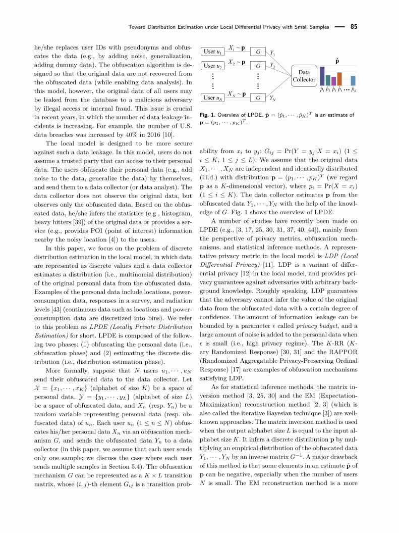
More formally, suppose that N users u1, · · · , uNsend their obfuscated data to the data collector. LetX = {x1, · · · , xK} (alphabet of size K) be a space ofpersonal data, Y = {y1, · · · , yL} (alphabet of size L)be a space of obfuscated data, and Xn (resp. Yn) be arandom variable representing personal data (resp. ob-fuscated data) of un. Each user un (1 ≤ n ≤ N) obfus-cates his/her personal dataXn via an obfuscation mech-anism G, and sends the obfuscated data Yn to a datacollector (in this paper, we assume that each user sendsonly one sample; we discuss the case where each usersends multiple samples in Section 5.4). The obfuscationmechanism G can be represented as a K × L transitionmatrix, whose (i, j)-th element Gij is a transition prob-
Data Collector
G
GUser u1 Y1
User u2 Y2
GUser uN YN
p~1X
p~2X
p~NX
p
1p 2p 3p 4p Kp
Fig. 1. Overview of LPDE. p = (p1, · · · , pK)T is an estimate ofp = (p1, · · · , pK)T .
ability from xi to yj : Gij = Pr(Y = yj |X = xi) (1 ≤i ≤ K, 1 ≤ j ≤ L). We assume that the original dataX1, · · · , XN are independent and identically distributed(i.i.d.) with distribution p = (p1, · · · , pK)T (we regardp as a K-dimensional vector), where pi = Pr(X = xi)(1 ≤ i ≤ K). The data collector estimates p from theobfuscated data Y1, · · · , YN with the help of the knowl-edge of G. Fig. 1 shows the overview of LPDE.
A number of studies have recently been made onLPDE (e.g., [3, 17, 25, 30, 31, 37, 40, 44]), mainly fromthe perspective of privacy metrics, obfuscation mech-anisms, and statistical inference methods. A represen-tative privacy metric in the local model is LDP (LocalDifferential Privacy) [11]. LDP is a variant of differ-ential privacy [12] in the local model, and provides pri-vacy guarantees against adversaries with arbitrary back-ground knowledge. Roughly speaking, LDP guaranteesthat the adversary cannot infer the value of the originaldata from the obfuscated data with a certain degree ofconfidence. The amount of information leakage can bebounded by a parameter ε called privacy budget, and alarge amount of noise is added to the personal data whenε is small (i.e., high privacy regime). The K-RR (K-ary Randomized Response) [30, 31] and the RAPPOR(Randomized Aggregatable Privacy-Preserving OrdinalResponse) [17] are examples of obfuscation mechanismssatisfying LDP.
As for statistical inference methods, the matrix in-version method [3, 25, 30] and the EM (Expectation-Maximization) reconstruction method [2, 3] (which isalso called the iterative Bayesian technique [3]) are well-known approaches. The matrix inversion method is usedwhen the output alphabet size L is equal to the input al-phabet size K. It infers a discrete distribution p by mul-tiplying an empirical distribution of the obfuscated dataY1, · · · , YN by an inverse matrixG−1. A major drawbackof this method is that some elements in an estimate p ofp can be negative, especially when the number of usersN is small. The EM reconstruction method is a more

Toward Distribution Estimation under Local Differential Privacy with Small Samples 86
sophisticated way to infer p. This method is based onthe EM algorithm [22], and iteratively estimates p untilconvergence. The feature of this method is that the finalestimate (converged value) p is equal to the ML (Max-imum Likelihood) estimate in the probability simplex(i.e., p1, · · · , pK ≥ 0,
∑Ki=1 pi = 1), irrespective of the
number of users N (see Section 3.2 for more details). Itis reported in [3] that the EM reconstruction methodsignificantly outperforms the matrix inversion method.
One of the main challenges in LPDE is how to ac-curately estimate the true discrete distribution p whenthe number of users N is small, or when users add alarge amount of noise to their personal data (i.e., highprivacy regime in which the privacy budget ε is small).It is well known that the ML estimate (i.e., the estimateby the EM reconstruction method) converges to the truevalue as the sample size goes to infinity. However, thenumber of users N can be small in practice due to var-ious reasons. For example, N can be small when a datacollector is a small-scale enterprise. Although Googleimplemented the RAPPOR in the Chrome browser andcollected a dozen million samples [17], small-scale enter-prises may not be able to collect such large samples. Foranother example, N can be small when a data collectorestimates a distribution for people at a certain place orat a certain time. Furthermore, even if N is large, theeffective sample size can be small in the high privacyregime. Duchi et al. [11] showed that for ε ∈ [0, 22
35 ],the effective sample size required to achieve a certainlevel of estimation errors (minimax rate) is 4ε2N (i.e.,it decreases quadratically with decrease in ε). Thus, itis very challenging to accurately estimate p when ε issmall (e.g., ε = 0.01 or 0.1).
1.1 Our Contributions
The goal of this paper is to accurately estimate a dis-crete distribution p when the number of users N or theprivacy budget ε is small. To achieve this goal, we fo-cus on a distribution estimation phase in LPDE. Specif-ically, we focus on the EM reconstruction method [2, 3],which is a state-of-the-art statistical inference method,and propose a method to correct its estimation error(i.e., difference between the estimate and the true value)to significantly improve the estimation accuracy.
Our contributions are summarized as follows:– We propose a method to correct an estimation error
of the EM reconstruction method based on the the-ory of Rilstone et al. [41]. A major problem here isthat the estimated error value may not be accurate
when N or ε is small. To address this issue, the pro-posed method multiplies the estimated error valueby a weight parameter α, and automatically deter-mines an optimal value of α. We also prove that theproposed method reduces the MSE (Mean SquareError) under some assumptions (Section 4).
– We evaluate the proposed method using three large-scale real datasets: the People-flow dataset [45], theFoursquare dataset [50], and the US Census (1990)dataset [33]. The first and second datasets con-tain location data, while the third dataset containscensus data. The results show that the proposedmethod significantly outperforms the existing in-ference methods (i.e., the matrix inversion method[3, 25, 30] and the EM reconstruction method [2, 3])in all of the datasets when N or ε is small (Sec-tion 5).
More specifically about the second contribution, we con-sider the fact that the required privacy level can varyfrom user to user in practice [29]. Conservative userswould require high level of privacy, whereas liberal userswould not mind low level of privacy. Some liberal usersmight not mind it even if some of their personal data(e.g., visited sightseeing places, innocuous responses ina survey) are made public, and consequently they mightnot use an obfuscation method.
Taking this into account, we evaluated the proposedmethod (denoted by Proposal) in a scenario where theprivacy budget ε is different from user to user (thosewho do not use an obfuscation method can be modeledby setting ε to ∞). We also generalize the matrix inver-sion method (denoted by MatInv) and the EM recon-struction method (denoted by EM) to such a scenario(see Section 3.2), and evaluate these methods for com-parison. The results show that Proposal outperformsMatInv and EM when the total number of users Nis small (e.g., N ≈ 1000) or when N is large but mostusers adopt a small value of ε (e.g., ε = 0.1).
In addition to the above-mentioned methods, wealso evaluate two methods that estimate p without theknowledge of the obfuscation mechanism. The first oneestimates p as an empirical distribution of the obfus-cated data Y1, · · · , YN (denoted by ObfDat). The sec-ond one always estimates p as a uniform distribution:p = ( 1
K , · · · ,1K )T (denoted by Uniform). In our exper-
iments, we show that all of Proposal, MatInv, andEM performed worse than these two methods whenboth N and ε (adopted by most users) are extremelysmall. This is because the variance of the estimate pis very small in ObfDat and Uniform (in particular,

Toward Distribution Estimation under Local Differential Privacy with Small Samples 87
the variance of p is always 0 in Uniform). On the otherhand, the variance of p is very large in Proposal,Mat-Inv, and EM when both N and ε are extremely small.We show this limitation, and provide a guideline forwhen to use the proposed method by thoroughly evalu-ating the effects of N and ε on the estimation accuracy.
2 Preliminaries
2.1 Notations
Table 1 shows the basic notations used in the rest of thispaper. It should be noted that we denote an obfuscationmechanism of user un by G(n) ∈ [0, 1]K×L (instead ofG). This is because the privacy budget ε can be differentfrom user to user, as described in Section 1.1.
Each user un (1 ≤ n ≤ N) obfuscates his/her per-sonal data Xn via the obfuscation mechanism G(n), andsends the obfuscated data Yn to a data collector (we dis-cuss the case where each user sends multiple samples inSection 5.4). The (i, j)-th element of G(n) is a transitionprobability from xi to yj : G(n)
i,j = Pr(Yn = yj |Xn = xi)(1 ≤ i ≤ K, 1 ≤ j ≤ L). The original data X1, · · · , XNare independent and identically distributed (i.i.d.) withdistribution p = (p1, · · · , pK)T ∈ [0, 1]K . We denote aset of all original data {X1, · · · , XN} and a set of all ob-fuscated data {Y1, · · · , YN} by X and Y, respectively.The data collector estimates p from Y with the helpof the knowledge of G(1), · · · , G(N). We denote the esti-mate of p by p = (p1, · · · , pK)T ∈ RK .
We also denote the probability simplex by C; i.e.,C := {p|p1, · · · , pK ≥ 0,
∑Ki=1 pi = 1}. Moreover, we
define the following K-dimensional vector:
gn := (G(n)1,π(Yn), · · · , G
(n)K,π(Yn))
T ∈ [0, 1]K , (1)
where π(Yn) is an index of the alphabet in Y that isequal to Yn (i.e., if Yn = yj , then π(Yn) = j). gn will beused in Sections 3.2 and 4.
2.2 Utility Metrics
In this paper, we use the MSE (Mean Square Error)and the JS (Jensen-Shannon) divergence [34] as utilitymetrics to measure the difference between the true dis-tribution p and its estimate p.
MSE (Mean Square Error). The MSE is one ofthe most popular metrics to measure the quality of an
Table 1. Basic notations used in this paper (1 ≤ n ≤ N).
Symbol DescriptionR Set of real numbers.N Number of users.un n-th user.X = {x1, · · · , xK} Space of original data.Y = {y1, · · · , yL} Space of obfuscated data.Xn n-th user’s original data.Yn n-th user’s obfuscated data.G(n) ∈ [0, 1]K×L n-th user’s obfuscation mechanism.X = {X1, · · · , XN} Set of all original data.Y = {Y1, · · · , YN} Set of all obfuscated data.p = (p1, · · · , pK)T Distribution of the original data.p = (p1, · · · , pK)T Estimate of p.C := {p|p1, · · · , pK ≥ 0,
∑K
i=1 pi = 1}(i.e., probability simplex).
π(Yn) index of the alphabet in Y equal to Yn(i.e., if Yn = yj , then π(Yn) = j).
gn := (G(n)1,π(Yn), · · · , G
(n)K,π(Yn))T .
estimator. Given p and p, the squared error (i.e., l2loss) is computed as follows:
||p− p||22 =K∑i=1
(pi − pi)2. (2)
It should be noted that the original data X are ran-domly generated from p, and the obfuscated data Yare randomly generated from X using the obfuscationmechanisms G(1), · · · , G(N). Since p is computed fromY, the squared error can be changed depending on Y.
The MSE is an expectation of the squared error:
MSE := E[||p− p||22] (3)
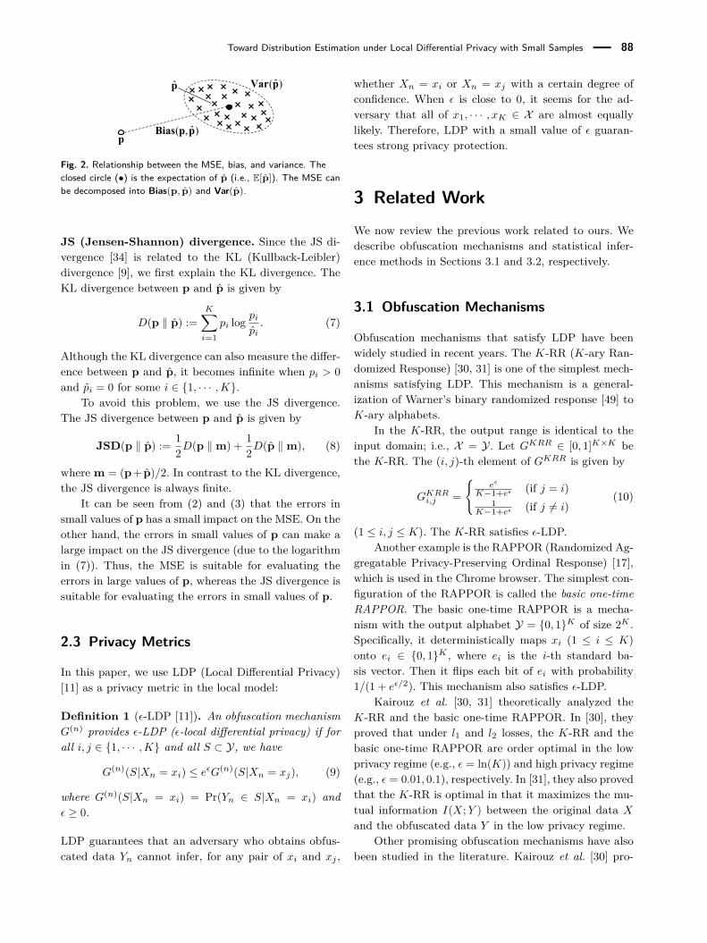
(or the sample mean of the squared errors over multiplerealizations of Y). Based on the bias-variance decompo-sition [22], it can be decomposed as follows:
MSE = ||Bias(p, p)||22 + Var(p), (4)
where
Bias(p, p) := E[p]− p (5)Var(p) := E[||p− E[p]||22]. (6)
Fig. 2 shows the relationship between the MSE,bias, and variance. Note that the bias and variance arehighly dependent on inference methods. For example,when we always estimate p as p = ( 1
K , · · · ,1K )T (i.e.,
Uniform), the variance is always 0 (i.e., Var(p) = 0).When we use the EM reconstruction method, the biasis much smaller (as shown in our experiments) and thevariance is larger than 0.
Toward Distribution Estimation under Local Differential Privacy with Small Samples 88
p
p
)ˆ(pVar
)ˆ,( ppBias
Fig. 2. Relationship between the MSE, bias, and variance. Theclosed circle (•) is the expectation of p (i.e., E[p]). The MSE canbe decomposed into Bias(p, p) and Var(p).
JS (Jensen-Shannon) divergence. Since the JS di-vergence [34] is related to the KL (Kullback-Leibler)divergence [9], we first explain the KL divergence. TheKL divergence between p and p is given by
D(p ‖ p) :=K∑i=1
pi log pipi. (7)
Although the KL divergence can also measure the differ-ence between p and p, it becomes infinite when pi > 0and pi = 0 for some i ∈ {1, · · · ,K}.
To avoid this problem, we use the JS divergence.The JS divergence between p and p is given by
JSD(p ‖ p) := 12D(p ‖m) + 1
2D(p ‖m), (8)
where m = (p+ p)/2. In contrast to the KL divergence,the JS divergence is always finite.
It can be seen from (2) and (3) that the errors insmall values of p has a small impact on the MSE. On theother hand, the errors in small values of p can make alarge impact on the JS divergence (due to the logarithmin (7)). Thus, the MSE is suitable for evaluating theerrors in large values of p, whereas the JS divergence issuitable for evaluating the errors in small values of p.
2.3 Privacy Metrics
In this paper, we use LDP (Local Differential Privacy)[11] as a privacy metric in the local model:
Definition 1 (ε-LDP [11]). An obfuscation mechanismG(n) provides ε-LDP (ε-local differential privacy) if forall i, j ∈ {1, · · · ,K} and all S ⊂ Y, we have
G(n)(S|Xn = xi) ≤ eεG(n)(S|Xn = xj), (9)
where G(n)(S|Xn = xi) = Pr(Yn ∈ S|Xn = xi) andε ≥ 0.
LDP guarantees that an adversary who obtains obfus-cated data Yn cannot infer, for any pair of xi and xj ,
whether Xn = xi or Xn = xj with a certain degree ofconfidence. When ε is close to 0, it seems for the ad-versary that all of x1, · · · , xK ∈ X are almost equallylikely. Therefore, LDP with a small value of ε guaran-tees strong privacy protection.
3 Related WorkWe now review the previous work related to ours. Wedescribe obfuscation mechanisms and statistical infer-ence methods in Sections 3.1 and 3.2, respectively.
3.1 Obfuscation Mechanisms
Obfuscation mechanisms that satisfy LDP have beenwidely studied in recent years. The K-RR (K-ary Ran-domized Response) [30, 31] is one of the simplest mech-anisms satisfying LDP. This mechanism is a general-ization of Warner’s binary randomized response [49] toK-ary alphabets.
In the K-RR, the output range is identical to theinput domain; i.e., X = Y. Let GKRR ∈ [0, 1]K×K bethe K-RR. The (i, j)-th element of GKRR is given by
GKRRi,j =
{eε
K−1+eε (if j = i)1
K−1+eε (if j 6= i)(10)
(1 ≤ i, j ≤ K). The K-RR satisfies ε-LDP.Another example is the RAPPOR (Randomized Ag-
gregatable Privacy-Preserving Ordinal Response) [17],which is used in the Chrome browser. The simplest con-figuration of the RAPPOR is called the basic one-timeRAPPOR. The basic one-time RAPPOR is a mecha-nism with the output alphabet Y = {0, 1}K of size 2K .Specifically, it deterministically maps xi (1 ≤ i ≤ K)onto ei ∈ {0, 1}K , where ei is the i-th standard ba-sis vector. Then it flips each bit of ei with probability1/(1 + eε/2). This mechanism also satisfies ε-LDP.
Kairouz et al. [30, 31] theoretically analyzed theK-RR and the basic one-time RAPPOR. In [30], theyproved that under l1 and l2 losses, the K-RR and thebasic one-time RAPPOR are order optimal in the lowprivacy regime (e.g., ε = ln(K)) and high privacy regime(e.g., ε = 0.01, 0.1), respectively. In [31], they also provedthat the K-RR is optimal in that it maximizes the mu-tual information I(X;Y ) between the original data Xand the obfuscated data Y in the low privacy regime.
Other promising obfuscation mechanisms have alsobeen studied in the literature. Kairouz et al. [30] pro-

Toward Distribution Estimation under Local Differential Privacy with Small Samples 89
posed the O-RR, which is an extension of the K-RR us-ing hash functions and cohorts. They showed that theperformance of the O-RR meets or exceeds that of K-RR and the basic one-time RAPPOR in both low andhigh privacy regimes. Sei et al. [44] proposed an exten-sion of the K-RR that not only randomizes the data butalso adds multiple dummy samples. They showed thatit outperforms the K-RR for ε ∈ [0.1, 1] using severalartificial datasets.
In this paper, we use the K-RR as an obfuscationmechanism satisfying LDP due to the following reasons:(1) it is simple and widely used; (2) the output alphabetsize L is small (not 2K but K); (3) it can provide theoptimal data utility in the low privacy regime [30, 31].
3.2 Statistical Inference Methods
The data collector computes an estimate p =(p1, · · · , pK)T of the distribution p based on obfus-cated data Y = {Y1, · · · , YN}. The matrix inver-sion method [3, 25, 30] and the EM reconstructionmethod [2, 3] are existing methods to compute pfrom Y. Although both of them assume that all usersu1, · · · , uN use the same obfuscation mechanism G
(= G(1) = · · · = G(N)), we generalize these methods tothe case where G(1), · · · , G(N) can be different, as wedescribe in detail below.
Matrix Inversion Method. Assume that the out-put alphabet size L is equal to the input alpha-bet size K, and that all users use the same obfus-cation mechanism G (= G(1) = · · · = G(N)). Letq = (q1, · · · , qK)T ∈ [0, 1]K be a distribution of ob-fuscated data, which is given by
qT = pTG. (11)
Let further q = (q1, · · · , qK)T ∈ [0, 1]K be an empiricaldistribution of Y. The matrix inversion method com-putes p by multiplying q by an inverse matrix G−1
pT = qTG−1. (12)
As the number of users N goes to infinity, the empiri-cal distribution q converges to the true distribution q.Therefore, p also converges to the true distribution p.
We generalize the matrix inversion method to thecase where there are multiple obfuscation mechanismsG1, · · · , GM (M � N) and each user chooses one of themechanisms to obfuscate his/her data (e.g., each userchooses one mechanism out of G1, G2, and G3, each
of which is corresponding to the high, middle, and lowprivacy regime, respectively). Let Nm (1 ≤ m ≤ M)be the number of users who use Gm (N =
∑Mm=1 Nm),
and qm ∈ [0, 1]K be an empirical distribution of theobfuscated data generated using Gm. Then, p can becomputed as follows:
pT = 1M
M∑n=1
qTmG−1m . (13)
As N1, · · · , NM go to infinity, p converges to p (in thesame way as the original matrix inversion method).
However, when the number of users N (=∑Mm=1 Nm) is small, many elements in p can be neg-
ative. Kairouz et al. [30] considered two methods toconstrain p to the probability simplex C. The firstmethod is a normalized decoder, which truncates thenegative elements of p to 0 and renormalizes p so thatthe sum is 1. The second method is a projected decoder,which projects p onto the probability simplex C so thatthe Euclidean distance between the two points is min-imized (using the algorithm in [48]). We evaluate bothmethods in Section 5.
EM reconstruction Method. The EM reconstruc-tion method is a more sophisticated method to inferp. It regards X as a latent variable (or hidden vari-able), and infers p from Y using the EM (Expectation-Maximization) algorithm [22], which guarantees thatthe log-likelihood function LY(p) := log Pr(Y|p) is in-creased at each iteration (EM cycle). Although thismethod assumes that mechanisms G(1), · · · , G(N) arethe same [2, 3], we describe this method in a generalcase where G(1), · · · , G(N) can be different.
Specifically, the following algorithm is equivalentto the EM algorithm (we can show this equivalence inthe same way as [2]; we omit the proof for lack of space):
Algorithm 1 (EM reconstruction Method):1. Initialize p = (p1, · · · , pK)T ∈ C (e.g., the empirical
distribution of Y can be used: p← q [3]).2. Compute p(new) = (p(new)
1 , · · · , p(new)K )T as follows:
p(new)k = 1
N
N∑n=1
pkG(n)k,π(Yn)∑K
l=1 plG(n)l,π(Yn)
. (14)
Repeat the update by (14) until convergence.
The feature of the EM reconstruction method is thatthe final estimate (converged value) p is equal to theML (Maximum Likelihood) estimate in the probabil-ity simplex C, irrespective of the number of users N .

Toward Distribution Estimation under Local Differential Privacy with Small Samples 90
This can be explained as follows. The ML estimate inthe probability simplex C maximizes the log-likelihoodfunction LY(p) (= log Pr(Y|p)) over C. Since all of theobfuscated data Y1, · · · , YN are independent, LY(p) canbe written, using Ln(p) := log Pr(Yn|p), as follows:
LY(p) =N∑n=1
Ln(p) =N∑n=1
log pTgn (15)
(note that Ln(p) = log Pr(Yn|p) = log∑Kk=1 pkG
(n)k,π(Yn)
= log pTgn). log pTgn is strictly concave in p, and thesum of strictly concave functions is strictly concave.Thus, LY(p) in (15) is strictly concave, and has a uniqueglobal maximum over C. It follows from (14) that the es-timate of the EM reconstruction method is always in C.In addition, each EM cycle in the EM algorithm is guar-anteed to increase LY(p) [22]. Therefore, the estimateof the EM reconstruction method converges to the MLestimate in C, whose log-likelihood is the global maxi-mum over C.
Note that this property holds irrespective of thenumber of users N . When N is small, many elementsof p can be negative in the matrix inversion method.On the other hand, the elements of p are always non-negative in the EM reconstruction method, since it isequal to the ML estimate in C. Thus, the EM recon-struction method can significantly outperform the ma-trix inversion method [3]. We also show this in Section 5.
4 Estimation Error Correction ofthe EM Reconstruction Method
The EM reconstruction method is a state-of-the-art sta-tistical inference method, whose estimate is equal to theML estimate in C, irrespective of the number of usersN . However, even this method may not accurately esti-mate the distribution p when N or ε is small, since theestimation error increases with decrease in N and ε.
To address this issue, we propose a method to re-duce an estimation error (i.e., difference between theestimate p and the true value p) of the EM reconstruc-tion method. Here we briefly describe its outline. Wefirst formalize the expectation of the estimation errorE[p]−p (i.e., bias) in the EM reconstruction method upto order O(N−1), which is denoted by a−1 ∈ RK , basedon the theory of Rilstone et al. [41]. We then replace theexpectation E in a−1 with the empirical mean over Nsamples Y1, · · · , YN . We denote the result value by a−1.It is important to note here that the estimate p is also
computed based on the N samples Y1, · · · , YN . Sinceboth a−1 and p are computed based on the N samplesY1, · · · , YN , we can regard a−1 as a rough approximationof p−p (i.e., estimation error vector), whereas a−1 ap-proximates E[p]−p. We also prove that, under some as-sumptions, the MSE of the EM reconstruction methodis reduced by subtracting a−1 from p (Proposition 1in Section 4.4). Note that this correction method wasused to reduce the bias of the estimate [5, 41]. How-ever, we prove a more general result that applying thiscorrection can lead to a reduction in the MSE.
The proposed method computes a−1 as an estimateof p−p, and subtracts it from p. However, a−1 may notbe accurately computed when N or ε is small. Thus, theproposed method multiplies a−1 by a weight parameterα and automatically determines an optimal value of α.
We first describe the theory of Rilstone et al. inSection 4.1. We then describe the proposed algorithm inSection 4.2, and describe how to determine an optimalvalue of α in Section 4.3. We finally provide a theoreticalanalysis of the MSE in Section 4.4.
4.1 Theory of Rilstone et al.
Given a set of N samples Y = {Y1, · · · , YN}, Rilstone etal. [41] considered an estimate p ∈ RK that is writtenas a solution to the following estimation equation:
N∑n=1
sn(p) = 0, (16)
where sn : RK → RK is a function that takes p as inputand outputs a K-dimensional vector based on the n-thsample Yn. The expectation of sn is 0 only at the truevalue p: E[sn(p)] = 0. The class of estimators charac-terized by (16) include the ML estimator, generalizedmethod of moments (GMM), and least squares (LS).
Rilstone et al. [41] showed that E[p]−p (i.e., bias) ofthe estimate that satisfies (16) can be written as follows:
E[p]− p = a−1 +O(N−3/2). (17)
a−1 ∈ RK is a dominant bias term of order O(N−1),which is called the second-order bias1, and is given by
a−1 = 1N
Q{E[VnQsn]− 1
2E[∇2sn]E[Qsn ⊗Qsn]},
(18)
1 Note that the first-order bias, which is a bias term of orderO(N−1/2), is given by E[−Qsn(p)] [41]. However, it is zero sinceE[sn(p)] = 0 (i.e., E[−Qsn(p)] = −QE[sn(p)] = 0).

Toward Distribution Estimation under Local Differential Privacy with Small Samples 91
where sn is a shorthand for sn(p), ∇ is a vector differ-ential operator (i.e., ∇ = ∂
∂p = ( ∂∂p1
, · · · , ∂∂pK
)), ⊗ is atensor product, and
Q = E[∇sn(p)]−1 ∈ RK×K (19)Vn = ∇sn(p)− E[∇sn(p)] ∈ RK×K . (20)
4.2 Proposed Algorithm
We now describe the proposed method. We first exploitthe fact that the estimate of the EM reconstructionmethod is equal to the ML estimate (as described inSection 3.2), and apply the theory of Rilstone et al. tothe EM reconstruction method.
Specifically, we exploit the fact that maximizing thelog-likelihood function LY(p) (=
∑Nn=1 Ln(p)) in (15)
is equivalent to solving the following equation:
N∑n=1∇Ln(p) = 0 (21)
(i.e., the gradient of the log-likelihood function ∇Ln is0). By regarding ∇Ln in (21) as sn in (16), we can applythe theory of Rilstone et al. to the EM reconstructionmethod.
Since Ln(p) = log pTgn (see (15)), sn (= ∇Ln),∇sn, and ∇2sn are written as follows:
sn(p) = 1pTgn
gn ∈ RK (22)
∇sn(p) = − 1(pTgn)2 gngTn ∈ RK×K (23)
∇2sn(p) = 1(pTgn)3 gn ⊗ gn ⊗ gn ∈ RK×K×K (24)
By using (23), Q in (19) and Vn in (20) are written asfollows:
Q = E[∇sn(p)]−1 = −E[
1(pTgn)2 gngTn
]−1(25)
Vn = ∇sn(p)− E[∇sn(p)] (26)
= E[
1(pTgn)2 gngTn
]− 1
(pTgn)2 gngTn . (27)
Note that −E[∇sn(p)] (= −E[∇2Ln(p)]) is the Fisherinformation matrix [9]. Since −Q is the inverse of thismatrix, it provides the lower bound of covariance matrix(i.e., Crámer-Rao inequality [9]).
The second-order bias a−1 in the EM reconstructionmethod is given by substituting (22), (24), (25), and(27) into (18). We replace the expectation E in a−1 withthe empirical mean over N samples Y1, · · · , YN . Since we
do not know the true value p, we also replace p with theestimate p (i.e., plug-in estimate), as done in [5, 41]. Theresult value, denoted by a−1, can be written as follows:
a−1 = 1N
Q
{1N
N∑n=1
(VnQsn(p))
− 12N2
N∑n=1
(∇2sn(p))N∑n=1
(Qsn(p)⊗ Qsn(p))
},
(28)
where
Q = −S−1 ∈ RK×K (29)
Vn = S− 1(pTgn)2 gngTn ∈ RK×K (30)
S = 1N
N∑n=1
1(pTgn)2 gngTn ∈ RK×K (31)
(E in a−1, Q, and Vn is now replaced by the empiricalmean in a−1, Q, and Vn, respectively). We emphasizeagain that both a−1 and p are computed based on theN samples Y1, · · · , YN . Therefore, we use a−1 as an es-timate of p− p (whereas a−1 approximates E[p]− p).
However, there is a major problem in computing Qin (29). When N or ε is small, the rank of S in (31)becomes much smaller than K (note that as ε goes to0, gngTn in (29) approaches to (1/K2)JK , where JK isthe K × K all-ones matrix whose rank is 1). When Sis highly rank deficient, we cannot compute Q in (29),which is the inverse of −S.
To avoid this problem, we add a small positive valueλ (> 0) to the diagonal elements of S to make S afull rank matrix. Such a regularization is known as theTikhonov regularization [20]. That is, we compute Q asfollows:
Q = −(S + λIK)−1 ∈ RK×K , (32)
where IK is the K ×K identity matrix.We compute a−1 from p and gn (1 ≤ n ≤ N) by
substituting (30), (31), and (32) into (28) (we can com-pute a−1 with time complexity O(NK2); for details, seeAppendix B). It should be noted, however, that Q in(32) may not be accurately computed, since the ma-trix λIK is added to S in (32). As a consequence, a−1may also not be accurately computed. To address thisissue, we multiply a−1 by a weight parameter α (> 0).In other words, we do not trust a−1 itself, but trust thedirection of a−1. We denote the corrected estimate inthe proposed method by p = (p1, · · · , pK)T ∈ RK ; i.e.,p = p−αa−1. We describe how to determine an optimalvalue of α in Section 4.3.
Toward Distribution Estimation under Local Differential Privacy with Small Samples 92
p
p
1ˆ ˆα
−= −p p aɶ
1ˆˆ
−− ap
Fig. 3. Corrected estimate p in the proposed method. We mul-tiply a−1 by α, and subtract it from an estimate p of the EMreconstruction method.
In summary, the proposed algorithm is as follows:
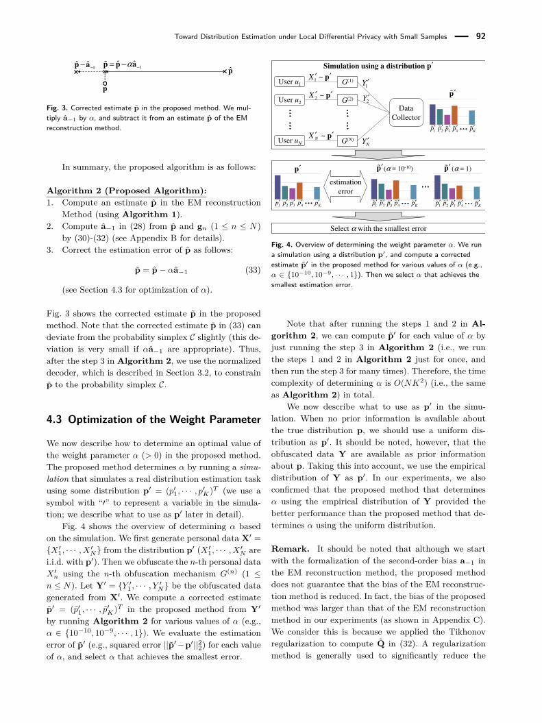
Algorithm 2 (Proposed Algorithm):1. Compute an estimate p in the EM reconstruction
Method (using Algorithm 1).2. Compute a−1 in (28) from p and gn (1 ≤ n ≤ N)
by (30)-(32) (see Appendix B for details).3. Correct the estimation error of p as follows:
p = p− αa−1 (33)
(see Section 4.3 for optimization of α).
Fig. 3 shows the corrected estimate p in the proposedmethod. Note that the corrected estimate p in (33) candeviate from the probability simplex C slightly (this de-viation is very small if αa−1 are appropriate). Thus,after the step 3 in Algorithm 2, we use the normalizeddecoder, which is described in Section 3.2, to constrainp to the probability simplex C.
4.3 Optimization of the Weight Parameter
We now describe how to determine an optimal value ofthe weight parameter α (> 0) in the proposed method.The proposed method determines α by running a simu-lation that simulates a real distribution estimation taskusing some distribution p′ = (p′1, · · · , p′K)T (we use asymbol with “′” to represent a variable in the simula-tion; we describe what to use as p′ later in detail).
Fig. 4 shows the overview of determining α basedon the simulation. We first generate personal data X′ ={X ′1, · · · , X ′N} from the distribution p′ (X ′1, · · · , X ′N arei.i.d. with p′). Then we obfuscate the n-th personal dataX ′n using the n-th obfuscation mechanism G(n) (1 ≤n ≤ N). Let Y′ = {Y ′1 , · · · , Y ′N} be the obfuscated datagenerated from X′. We compute a corrected estimatep′ = (p′1, · · · , p′K)T in the proposed method from Y′
by running Algorithm 2 for various values of α (e.g.,α ∈ {10−10, 10−9, · · · , 1}). We evaluate the estimationerror of p′ (e.g., squared error ||p′−p′||22) for each valueof α, and select α that achieves the smallest error.
1Y ′
2Y ′
NY ′
Data
Collector
G(2)
G(1)User u1
User u2
G(N)User uN
p′′ ~1X
p′′ ~2X
p′′ ~NX
′pɶp′
1p′2p′
3p′4p′
Kp′
(α = 10-10) ′pɶ (α = 1)
estimation
error
′pɶ
1p′ɶ
2p′ɶ
Select α with the smallest error
Simulation using a distribution p′
3p′ɶ
4p′ɶ
Kp′ɶ
1p′ɶ
2p′ɶ
3p′ɶ
4p′ɶ
Kp′ɶ
1p′ɶ
2p′ɶ
3p′ɶ
4p′ɶ
Kp′ɶ
Fig. 4. Overview of determining the weight parameter α. We runa simulation using a distribution p′, and compute a correctedestimate p′ in the proposed method for various values of α (e.g.,α ∈ {10−10, 10−9, · · · , 1}). Then we select α that achieves thesmallest estimation error.
Note that after running the steps 1 and 2 in Al-gorithm 2, we can compute p′ for each value of α byjust running the step 3 in Algorithm 2 (i.e., we runthe steps 1 and 2 in Algorithm 2 just for once, andthen run the step 3 for many times). Therefore, the timecomplexity of determining α is O(NK2) (i.e., the sameas Algorithm 2) in total.
We now describe what to use as p′ in the simu-lation. When no prior information is available aboutthe true distribution p, we should use a uniform dis-tribution as p′. It should be noted, however, that theobfuscated data Y are available as prior informationabout p. Taking this into account, we use the empiricaldistribution of Y as p′. In our experiments, we alsoconfirmed that the proposed method that determinesα using the empirical distribution of Y provided thebetter performance than the proposed method that de-termines α using the uniform distribution.
Remark. It should be noted that although we startwith the formalization of the second-order bias a−1 inthe EM reconstruction method, the proposed methoddoes not guarantee that the bias of the EM reconstruc-tion method is reduced. In fact, the bias of the proposedmethod was larger than that of the EM reconstructionmethod in our experiments (as shown in Appendix C).We consider this is because we applied the Tikhonovregularization to compute Q in (32). A regularizationmethod is generally used to significantly reduce the

Toward Distribution Estimation under Local Differential Privacy with Small Samples 93
variance by introducing a bias in the estimate. TheTikhonov regularization can also introduce a bias [28].
However, we emphasize that the goal of this paperis to accurately estimate p when N or ε is small, andthat we utilize a−1 as a means to reduce the estimationerror. In our experiments, we show that it significantlyreduces the variance (at the cost of increasing the bias),and therefore reduces the MSE and the JS divergence.We also prove that the proposed method reduces theMSE under some assumptions in Section 4.4.
It should also be noted that the weight parameterα can influence the estimation accuracy. In this paper,we generate artificial data from the empirical distribu-tion of Y in an analogous way to the parametric boot-strap method [15], and chooses a hyper-parameter α(i.e., performs a kind of model selection) using the arti-ficial data. It is also known that the bootstrap methodis used for model selection [27]. However, we may beable to choose a better α by improving our method inseveral directions. For example, although we choose αthat minimizes the squared error ||p′ − p′||22 based onone simulation in our experiments, we may be able tochoose a better α by running multiple simulations andusing the MSE as a metric (at the cost of computa-tional time necessary to optimize α). We may also beable to choose a better α by extending our method tothe Bayesian framework in the same way as [19]. Weleave such improvements as future work.
4.4 Theoretical Analysis
We provide a theoretical analysis of the MSE in the pro-posed method. Specifically, we show that the proposedmethod can reduce the second-order MSE, which is anMSE term of order O(N−3/2), to zero under some as-sumptions.
According to the theory of Rilstone et al. [41], theMSE of the EM reconstruction method (denoted byMSEEM) can be written as follows2:
MSEEM = b−1 + b−3/2 +O(N−2), (34)
where
b−1 = E[dTd
]∈ R (35)
b−3/2 = −E[dT{
2QVnd−QE[∇2sn][d⊗ d]}]∈ R(36)
2 Note that in [41], the MSE is represented in the form of amatrix (i.e., error covariance matrix). MSEEM can be writtenas (34) by computing the trace of the MSE matrix in [41].
d = 1N
N∑n=1
dn ∈ RK (37)
dn = Qsn ∈ RK . (38)
b−1 is a term of order O(N−1), and is called the first-order MSE. b−3/2 is a term of order O(N−3/2), and iscalled the second-order MSE.
We now consider the proposed method with theweight parameter α = 1, which corrects the estimatep of the EM reconstruction method by subtracting a−1in (28) from p:
p = p− a−1 (39)
Let MSEProposal be the MSE of this method. Tosimplify our theoretical analysis, we assume the follow-ing two assumptions: (i) a−1 is evaluated at p, (ii)Q, Vn, and E[∇2sn] are perfectly estimated: Q = Q,Vn = Vn, and E[∇2sn] = 1
N
∑Nn=1(∇2sn). In this case,
a−1 in (28) can be written as follows:
a−1 = 1N
Q
{1N
N∑n=1
(VnQsn)
− 12N E[∇2sn]
N∑n=1
(Qsn ⊗Qsn)
}. (40)
It should be noted that although we make some idealassumptions, we still replace the two expectation termsE in a−1 (see (18)) with the empirical mean over N sam-ples Y1, · · · , YN . We prove that the second-order MSE isreduced to zero by these replacements.
Namely, we prove the following result:
Proposition 1.
MSEProposal = b−1 +O(N−2). (41)
The proof is given in Appendix A. Proposition 1 indi-cates that the estimation error can be reduced by sub-tracting a−1 from p (since a−1 may not be accuratelycomputed, we multiply a−1 by α in practice). It shouldbe noted, however, that the first-order MSE b−1 is notreduced in this case. This can be explained by the factthat Proposal provides almost the same performanceas EM when N is large in our experiments. However,we emphasize that it is still beneficial to reduce b−3/2when N is small, since the term of order O(N−3/2) islarge in this case. In fact, Proposal significantly out-performs EM when N or ε is small, as shown in ourexperiments.

Toward Distribution Estimation under Local Differential Privacy with Small Samples 94
5 Experimental Evaluation
5.1 Experimental Set-up
We evaluated the proposed method by conducting ex-periments using three real datasets: the People-flowdataset [45], the Foursquare dataset [50], and the USCensus (1990) dataset [33]. The first two datasets con-tain location data, while the third dataset contains cen-sus data. We used these datasets because they are large-scale datasets (we used the data of 303916, 251689, and2458285 people in the People-flow, Foursquare, and USCensus datasets, respectively). In the following, we de-scribe these datasets in detail:– People-flow dataset: The People-flow dataset
(1998 Tokyo metropolitan area) [45] contains mo-bility traces (time-series location trails) of 722000people in the Tokyo metropolitan area in 1998. Inthis paper, we used this dataset for estimating ageographic population distribution in the period ofone day. To this end, we extracted mobility tracesof 303916 people on the first of October, and usedthe first location sample for each user (we excludedthe remaining 418084 people since they had no lo-cation samples on the first of October). We dividedthe Tokyo metropolitan area into 20×20 regions, ex-cluded 119 regions in the sea, and used the remain-ing 281 land regions as input alphabets (K = 281).
– Foursquare dataset: The Foursquare dataset(global-scale check-in dataset) [50] was collectedfrom April 2012 to September 2013. It containslocation check-ins by 266909 people all over theworld. Since many of these check-ins were located in415 cities, we focused on these cities. We extracted251689 people who had at least one check-in in thesecities, and used the first location check-in for eachuser (we excluded the remaining 15220 people whohad no check-ins in these cities). We used the 415cities as input alphabets (K = 415).
– US Census (1990) dataset: The US Census(1990) dataset [33] was collected as part of US cen-sus in 1990. It contains responses from 2458285 peo-ple (each user provided one response), where eachresponse has 68 attributes. We used the responsesfrom all people, and used age, sex, income, and mar-ital status as attributes. Each attribute has 8, 2,5, and 5 category IDs depending on their value, asshown in Table 2. We regarded a sequence of thesecategory IDs as a single category ID. Thus, the to-tal number of category IDs is 400 (= 8× 2× 5× 5).
Table 2. Attributes (age, sex, income, and marital status) andcategory IDs in the US Census (1990) dataset.
Attribute Category ID (Value)Age 0 (0), 1 (1-12), 2 (13-19), 3 (20-29),
4 (30-39), 5 (40-49), 6 (50-64), or 7 (65-)Sex 0 (male) or 1 (female)Income 0 ($0), 1 ($1-$14999), 2 ($15000-$29999),
3 ($30000-$60000), or 4 ($60000-)Marital status 0 (now married, except separated),
1 (widowed), 2 (divorced),3 (separated), or 4 (never married)
We used these category IDs as input alphabets(K = 400).
For each dataset, we used a frequency distribution ofall people (303916, 251689, and 2458285 people in thePeople-flow, Foursquare, and US Census datasets, re-spectively) as p (i.e., distribution of the original data).We randomly selected N users from these people. Herewe attempted 100 cases to randomly select N users, andran, for each case, the following experiments.
We conducted experiments, in which each user un(1 ≤ n ≤ N) obfuscates his/her personal data Xn (i.e.,region ID, city ID, or category ID) via the obfuscationmechanism G(n), and a data collector computes an es-timate p of the distribution p based on the obfuscateddata Y = {Y1, · · · , YN}. As an obfuscation mechanismG(n), we used the K-RR (i.e., GKRR in (10)). As forthe privacy budget ε, we considered four values: ε = 0.1,2, ln(K), and ∞, each of which is corresponding to thehigh, middle, low, and “no” privacy regime, respectively.We denote the number of users who set ε = 0.1, 2,ln(K), and ∞ by N1, N2, N3, and N4, respectively (i.e.,N =
∑4i=1 Ni).
We set ε = 0.1 and 2 in the high and middle pri-vacy regime, respectively, since many studies used thesevalues [24] and ε = 0.1 offers reasonably strong privacyprotection [32]. We set ε = ln(K) in the low privacyregime, since a user sends different data (i.e., Xn 6= Yn)with probability 50% even in this case. In other words,ε = ln(K) can still provide plausible deniability. Thisvalue of ε was also used in [30]. When ε =∞, GKRR in(10) is equivalent to the identity matrix IK . This meansthat those who do not use an obfuscation method can bemodeled by setting ε to ∞, as described in Section 1.1.
However, many users might care about their pri-vacy and prefer the high or middle privacy regime (i.e.,ε = 0.1 or 2). Taking this into account, we set N3 andN4 much smaller than N1 and N2. Specifically, we firstset N1, N2, N3, and N4 so that N1 : N2 : N3 = 10 : 10 : 1

Toward Distribution Estimation under Local Differential Privacy with Small Samples 95
and changed N4 from 0 to N3 (e.g., (N1, N2, N3) =(500, 500, 50) and N4 ∈ [0, 50]). We then evaluated theperformance in the case where we significantly increasedonly N1 (i.e., most users select the high privacy regimein which ε = 0.1). To more thoroughly evaluate theeffects of N and ε on the performance, we also setN1 = N4 = 0 and evaluated the performance for var-ious values of N2 and N3.
As a statistical inference method, we evaluated thefollowing methods for comparison:– Uniform: A method that always estimates p as a
uniform distribution: p = ( 1K , · · · ,
1K )T .
– ObfDat: A method that estimates p as an empiri-cal distribution of the obfuscated data Y1, · · · , YN .
– MatInvnorm: The matrix inversion method usingthe normalized decoder (described in Section 3.2).
– MatInvproj: The matrix inversion method usingthe projected decoder (described in Section 3.2).
– EM: The EM reconstruction method (described inSection 3.2).
– Proposal: The proposed method.
In EM, we used the empirical distribution of Y as aninitial value of p (i.e., p ← q) in the same way as [3].In Proposal, we set λ = 10−3, and attempted vari-ous values for α: α ∈ {c1 × 10c2 |c1 ∈ {1, · · · , 9}, c2 ∈{−1, · · · ,−10}}. Then we selected α that achieved thesmallest squared error (i.e., ||p′ − p′||22).
After computing the estimate p (or the correctedestimate p in Proposal), we evaluated the MSE andthe JS divergence. Specifically, we computed the aver-age of the squared error ||p−p||22 (or ||p−p||22) over 100runs (i.e., 100 cases to randomly select N users), andused it as the MSE. In other words, we computed thesample mean of 100 squared errors as the MSE. Simi-larly, we averaged the JS divergence over 100 runs. Wealso evaluated, for both the squared error and the JSdivergence, the standard deviation over 100 runs.
5.2 Experimental Results
We first evaluated the MSE and the JS divergence inthe case where (N1, N2, N3) = (500, 500, 50) and N4 ∈[0, 50]. Fig. 5 shows the results.
It can be seen that the MSE and the JS divergenceof MatInvnorm and MatInvproj are very large. Thisis because many elements in the estimate p were nega-tive, as described in Section 3.2. In particular, the per-formance of MatInvproj is much worse than that of theother inference methods. This is because the estimate p
(i) People-flow dataset ((N1, N2, N3) = (500, 500, 50))
0.1
0.2
0.3
0.4
0.5
0.6
0.7
0 20 40 60 80 100N4
JS D
iver
genc
e
4.0E-03
9.0E-03
1.4E-02
1.9E-02
2.4E-02
2.9E-02
8.0E-01
1.2E+00
0 10 20 30 40 50
MSE
N4
Uniform ObfDat MatInvnorm EM ProposalMatInvproj
(ii) Foursquare dataset ((N1, N2, N3) = (500, 500, 50))
0.1
0.2
0.3
0.4
0.5
0.6
0.7
0 20 40 60 80 100N4
JS D
iver
genc
e
4.0E-03
9.0E-03
1.4E-02
1.9E-02
2.4E-02
2.9E-02
8.0E-01
1.2E+00
0 10 20 30 40 50
MSE
N4
Uniform ObfDat MatInvnorm EM ProposalMatInvproj
(iii) US Census dataset ((N1, N2, N3) = (500, 500, 50))
6.0E-03
1.2E-02
1.8E-02
2.4E-02
3.0E-02
3.6E-02
7.0E-01
1.2E+00
0 10 20 30 40 50
MSE
N4
0 20 40 60 80 100N4
JS D
iver
genc
e
0.18
0.27
0.36
0.45
0.54
0.63
0.72
Uniform ObfDat MatInvnorm EM ProposalMatInvproj
Fig. 5. The MSE and the JS divergence in the case where(N1, N2, N3) = (500, 500, 50) and N4 ∈ [0, 50]. The error barsshow standard deviations (we do not show error bars in Uniformand ObfDat, since the standard deviations are very small in thesemethods; in particular, the standard deviation is 0 in Uniform).
that contained many negative elements was projectedto a vertex of the probability simplex (i.e., each elementin p was either 0 or 1). On the other hand, EM outper-forms MatInvnorm and MatInvproj in most cases (inthe same way as [3]), since the elements in p are alwaysnonnegative, as described in Section 3.2.
It can also be seen that Proposal outperforms EM,which shows that the estimation accuracy is improvedby correcting the estimation error (although the errorbars overlap in many cases, we show later that there isa very high correlation between 100 squared errors ofProposal and those of EM). In particular, Proposalsignificantly outperforms EM when N4 is small. This isbecause the estimation error of EM is large in this caseand is corrected by Proposal.
However, when N4 is small, Uniform or ObfDatprovides the best performance in some cases (e.g., theMSE in the People-flow dataset, the JS divergence in

Toward Distribution Estimation under Local Differential Privacy with Small Samples 96
(i) People-flow dataset
0.1
0.2
0.3
0.4
0.5
0.6
0.8
JS D
iver
genc
e
MSE
N
0.7
N
4.0E-03
1.0E-02
1.6E-02
2.2E-02
2.8E-02
3.4E-02
8.0E-01
1.2E+00
Uniform ObfDat MatInvnorm EM ProposalMatInvproj
(ii) Foursquare datasetJS
Div
erge
nce
MSE
N
2.0E-03
8.0E-03
1.4E-02
2.0E-02
2.6E-02
3.2E-02
6.0E-01
1.2E+00
0.05
0.15
0.25
0.35
0.45
0.55
0.75
0.65
N
Uniform ObfDat MatInvnorm EM ProposalMatInvproj
(iii) US Census dataset
JS D
iver
genc
e
MSE
5.0E-03
1.7E-02
2.9E-02
4.1E-02
5.3E-02
6.5E-02
5.0E-01
1.2E+00
0.1
0.2
0.3
0.4
0.5
0.6
0.8
0.7
N N
Uniform ObfDat MatInvnorm EM ProposalMatInvproj
Fig. 6. The MSE and the JS divergence in the case where N ischanged while fixing N1 : N2 : N3 : N4 = 10 : 10 : 1 : 1. Theerror bars show standard deviations.
the Foursquare dataset). This is because the variance ofthe estimate p was very small in Uniform and Obf-Dat (in Appendix C, we also show the results of thebias and variance for each method; see Appendix C fordetails). More specifically, the variance of p was always0 in Uniform, as described in Section 2.2. The vari-ance of p was also close to 0 in ObfDat, since only asmall number of people sent the original data Xn (i.e.,Xn = Yn). In other words, the empirical distributionof the obfuscated data Y1, · · · , YN was close to the uni-form distribution. If the variance is larger than the biasof these methods, the MSE is also larger.
To investigate the relationship between the totalnumber of users N (=
∑4i=1 Ni) and the performance,
we changed N while fixing the ratio of N1 : N2 : N3 : N4.Specifically, we changed N while fixing N1 : N2 : N3 :N4 = 10 : 10 : 1 : 1. Fig. 6 shows the results. It canbe seen that when N is very small, the MSE of Uni-
(i) People-flow dataset ((N1, N2, N3) = (20000, 500, 50))
0.1
0.2
0.3
0.4
0.5
0.6
0.7
0 20 40 60 80 100N4
JS D
iver
genc
e
4.0E-03
9.0E-03
1.4E-02
1.9E-02
2.4E-02
2.9E-02
8.0E-01
1.2E+00
0 10 20 30 40 50
MSE
N4
Uniform ObfDat MatInvnorm EM ProposalMatInvproj
(ii) Foursquare dataset ((N1, N2, N3) = (20000, 500, 50))
0.1
0.2
0.3
0.4
0.5
0.6
0.7
0 20 40 60 80 100N4
JS D
iver
genc
e
4.0E-03
9.0E-03
1.4E-02
1.9E-02
2.4E-02
2.9E-02
8.0E-01
1.2E+00
0 10 20 30 40 50
MSE
N4
Uniform ObfDat MatInvnorm EM ProposalMatInvproj
(iii) US Census dataset ((N1, N2, N3) = (20000, 500, 50))
6.0E-03
1.2E-02
1.8E-02
2.4E-02
3.0E-02
3.6E-02
7.0E-01
1.2E+00
0 10 20 30 40 50
MSE
N4
0 20 40 60 80 100N4
JS D
iver
genc
e
0.18
0.27
0.36
0.45
0.54
0.63
0.72
Uniform ObfDat MatInvnorm EM ProposalMatInvproj
Fig. 7. The MSE and the JS divergence in the case where N1 =20000. The error bars show standard deviations.
form or ObfDat is the smallest in all of the datasets.It can also be seen that the MSE and the JS diver-gence of Proposal rapidly decrease as N increases.Proposal provides the best performance with respectto both the MSE and the JS divergence when N is morethan or equal to 660, 1320, and 440 in the People-flow,Foursquare, and US Census datasets, respectively.
We also evaluated the performance in the case wherewe significantly increased only N1 (i.e., the number ofusers with ε = 0.1). Specifically, we set (N1, N2, N3) =(20000, 500, 50) and N4 ∈ [0, 50]. Fig. 7 shows the re-sults. Fig. 7 is very similar to Fig. 5, and the MSE andthe JS divergence are only slightly decreased (or not de-creased) by increasing N1. This is because when ε = 0.1,the probability of sending the original data Xn (i.e.,Xn = Yn) was very small (0.39%, 0.27%, and 0.28%, inthe People-flow, Foursquare, and US Census datasets,respectively). Since these users sent different data (i.e.,Xn 6= Yn) in most cases, they did not contribute muchto the estimation accuracy. This is consistent with the

Toward Distribution Estimation under Local Differential Privacy with Small Samples 97
200EM PR
N2
10-2
Squa
red
Erro
r
People-flow (N3 = 0)16
14
1210
8
6
4
400EM PR
600EM PR
0EM PR
200EM PR
400EM PR
600EM PR
22201816141210
N2
10-3
Squa
red
Erro
r
People-flow (N3 = 100)
0EM PR
200EM PR
400EM PR
600EM PR
N2
Squa
red
Erro
r
10-3 People-flow (N3 = 200)1413121110
9876
0EM PR
200EM PR
400EM PR
600EM PR
N2
Squa
red
Erro
r
10-3 People-flow (N3 = 300)111098765
200EM PR
N2
10-2
Squa
red
Erro
r
Foursquare (N3 = 0)
400EM PR
600EM PR
161412108642
0EM PR
200EM PR
400EM PR
600EM PR
N2
10-3Sq
uare
d Er
ror
Foursquare (N3 = 100)
22201816141210
24
86
0EM PR
200EM PR
400EM PR
600EM PR
N2
Squa
red
Erro
r
10-3 Foursquare (N3 = 200)16
14
12
10
8
6
0EM PR
200EM PR
400EM PR
600EM PR
N2
Squa
red
Erro
r
10-3 Foursquare (N3 = 300)
1110987654
1312
200EM PR
N2
10-2
Squa
red
Erro
r
US Census (N3 = 0)
400EM PR
600EM PR
16141210
864
18
0EM PR
200EM PR
400EM PR
600EM PR
N2
10-2
Squa
red
Erro
r
US Census (N3 = 30)
5.56
4.55
3.54
2.53
1.52
0EM PR
200EM PR
400EM PR
600EM PR
N2
Squa
red
Erro
r
10-2 US Census (N3 = 60)
3.5
3
2.5
2
1.5
1
0EM PR
200EM PR
400EM PR
600EM PR
N2
Squa
red
Erro
r
10-2 US Census (N3 = 90)3
2.5
2
1.5
1
Fig. 8. Box plots of 100 squared errors for EM and Proposal in the case where N2 and N3 are changed and N1 = N4 = 0 (EM: EM,PR: Proposal). The ends of the whiskers represent the minimum and maximum values. The bottom and top of the box represent thefirst and third quartiles, respectively. The red band inside the box represents the median.
fact that the effective sample size decreases quadrati-cally with decrease in ε [11].
To more thoroughly evaluate the effects of N andε on the performance, we finally set N1 = N4 = 0 andevaluated 100 squared errors and the MSE for variousvalues of N2 and N3 (we do not show the JS divergencefor lack of space). Fig. 8 shows the box plots of 100squared errors for EM and Proposal. We also com-puted the correlation coefficient r between 100 squarederrors of Proposal and those of EM, and the p-value pof the t-test for paired samples. Fig. 9 shows the results.In addition, Fig. 10 shows the best inference method,which achieves the smallest MSE among the six meth-ods, for each case.
It can be seen from Fig. 8 that Proposal signifi-cantly outperforms EM when N3 is small. This is be-cause the estimation error of EM is large in this caseand is corrected by Proposal. It can also be seen fromFig. 9 that the correlation coefficient r is very closeto one in most cases. This means that when the MSEof Proposal is smaller than that of EM, Proposaloutperforms EM in almost all of the 100 runs. Con-
sequently, the difference between 100 squared errors ofProposal and those of EM is statistically significant(p < 0.05).
However, it can be seen from Fig. 10 that Uniformor ObfDat provides the best performance when N2 andN3 are very small (e.g., N3 = 0). This is because thevariance of the estimate p was very small in UniformandObfDat, as previously explained. In addition, Pro-posal provides almost the same performance as EMwhen N2 and N3 are large. From Fig. 8 and 10, we con-clude that Proposal is effective especially when N3 isabout 100 to 200 in the People-flow dataset, about 100to 200 in the Foursquare dataset, and about 30 to 60 inthe US Census dataset.
5.3 Visualization of Distributions
In Section 5.2, Proposal significantly outperformedEM in the case where the number of users N was smallor when most users adopted a small value of ε. To ex-plain how the proposed method corrected the estimation

Toward Distribution Estimation under Local Differential Privacy with Small Samples 98
r = 0.999p = 9.90×10⁻³⁵
r = 0.994p = 8.78×10⁻³⁴
r = 0.989p = 6.69×10⁻²⁴
r = 0.982p = 3.06×10⁻²¹
r = 0.999p = 1.23×10-45
r = 0.991p = 1.96×10-42
r = 0.982p = 3.98×10-41
r = 0.975p = 2.55×10-38
r = 0.999p = 3.69×10-61
r = 0.974p = 7.65×10-64
r = 0.955p = 1.69×10-57
r = 0.956p = 4.80×10-65
N/A r = 0.970p = 5.90×10-45
r = 0.966p = 1.54×10-67
r = 0.964p = 1.04×10-70
N3
0 200 400 600 N2
(i) People-flow dataset
0
100
200
300
r = 0.999p = 8.93×10⁻⁹
r = 0.997p = 6.88×10-41
r = 0.996p = 5.38×10-42
r = 0.987p = 1.14×10⁻²⁸
r = 0.999p = 6.48×10⁻²⁰
r = 0.994p = 3.85×10-46
r = 0.986p = 1.49×10-44
r = 0.990p = 3.92×10-48
r = 0.999p = 9.50×10-50
r = 0.966p = 2.46×10-56
r = 0.968p = 1.14×10-62
r = 0.974p = 2.83×10-66
N/A r = 0.999p = 3.62×10-70
r = 0.996p = 1.14×10-69
r = 0.982p = 2.59×10-76
N3
0 200 400 600 N2
(ii) Foursquare dataset
0
100
200
300
r = 0.999p = 1.46×10⁻²²
r = 0.988p = 6.62×10-41
r = 0.981p = 2.91×10⁻³⁴
r = 0.946p = 3.26×10⁻²⁷
r = 0.999p = 3.09×10-49
r = 0.980p = 1.61×10-58
r = 0.966p = 1.37×10-52
r = 0.899p = 2.75×10-43
r = 0.999p = 1.05×10-72
r = 0.964p = 4.50×10-75
r = 0.940p = 7.40×10-67
r = 0.918p = 9.48×10-70
N/A r = 0.999p = 1.58×10-63
r = 0.995p = 8.96×10-68
r = 0.984p = 1.01×10-73
N3
0 200 400 600 N2
(iii) US Census dataset
0
30
60
90
Fig. 9. Correlation coefficients and p-values in the case whereN2 and N3 are changed and N1 = N4 = 0. “r” represents thecorrelation coefficient between 100 squared errors of Proposaland those of EM. “p” represents the p-value of the t-test forpaired samples.
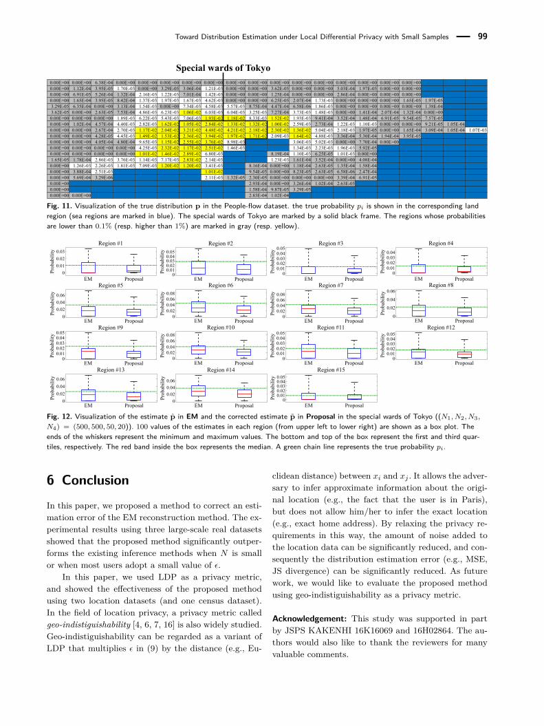
error in the EM reconstruction method, we visualize thetrue distribution p, the estimate p in EM, and the cor-rected estimate p in Proposal using the People-flowdataset.
Fig. 11 shows the true distribution p. Fig. 12 showsp and p in the special wards of Tokyo in the case where(N1, N2, N3, N4) = (500, 500, 50, 20). In Fig. 12, we show100 values of the estimates in each of the fifteen regions(from upper left to lower right) as a box plot.
It can be seen that a variance of is smaller in Pro-posal in all of the regions. The maximum value of pi inEM is much larger than the true value. EM also esti-mates pi to be very close to zero in many cases (e.g., Re-gions #1, #3, #4, and #15). Proposal corrects theseover/underestimated values. We consider this is the rea-son Proposal significantly outperformed EM.
5.4 Discussions on the Case of MultipleSamples Per User
In our experiments, we assumed that each user sendsonly one sample, and the data collector estimates the
MatInvnorm(7.38×10⁻³)
Proposal (7.48×10⁻³)
Proposal (7.24×10⁻³)
Proposal(7.43×10⁻³)
ObfDat(9.48×10⁻³)
Proposal(9.25×10⁻³)
Proposal(8.89×10⁻³)
Proposal(9.00×10⁻³)
ObfDat(1.45×10⁻²)
Proposal(1.26×10⁻²)
Proposal(1.22×10⁻²)
Proposal(1.23×10⁻²)
N/A Uniform(1.59×10⁻²)
Uniform(1.59×10⁻²)
Uniform(1.59×10⁻²)
N3
0 200 400 600 N2
(i) People-flow dataset
0
100
200
300
Proposal(6.25E-03)
Proposal(5.99E-03)
Proposal(6.02E-03)
Proposal(5.86E-03)
Proposal(8.05E-03)
Proposal(7.82E-03)
Proposal(7.49E-03)
Proposal(7.52E-03)
Proposal(1.34E-02)
Proposal(1.17E-02)
Proposal(1.09E-02)
Proposal(1.09E-02)
N/A Uniform(1.46E-02)
Uniform(1.46E-02)
Uniform(1.46E-02)
N3
0 200 400 600 N2
(ii) Foursquare dataset
0
100
200
300
Proposal(1.70E-02)
Proposal(1.60E-02)
Proposal(1.55E-02)
Proposal(1.57E-02)
Proposal(2.28E-02)
Proposal(1.95E-02)
Proposal(1.85E-02)
Proposal(1.85E-02)
Uniform(2.59E-02)
Uniform(2.59E-02)
Proposal(2.55E-02)
Proposal(2.48E-02)
N/A Uniform(2.59E-02)
Uniform(2.59E-02)
Uniform(2.59E-02)
N3
0 200 400 600 N2
(iii) US Census dataset
0
30
60
90
Fig. 10. Best inference method, which achieves the smallestMSE, in the case where N2 and N3 are changed and N1 = N4 =0. The value inside of the parenthesis represents the MSE. A cellin which Proposal is not the best method is shaded in gray.
distribution p. We finally discuss the extension of ourresults to case where each user sends multiple samples.
For example, suppose that user un obfuscates t sam-ples X
(1)n , · · · , X(t)
n using the obfuscation mechanismG(n), which satisfies ε-LDP, and sends the obfuscatedsamples Y (1)
n , · · · , Y (t)n to the data collector. Then, it
follows from by the composition theorem [13] that the tsamples are protected by (εt)-LDP. Therefore, if user unwants to protect t samples by ε-LDP, he/she can satisfythis privacy requirement by using, for each sample, theobfuscation mechanism satisfying (ε/t)-LDP.
When the number of samples t is large, each pri-vacy budget ε/t can be very small and therefore a largeamount of noise is added to each sample. A recent study[38] also showed that the data utility can be completelydestroyed in the case of time-series location data. Itshould be noted, however, that the number of samples tcan be different from user to user, and ε/t can be largefor users whose t is small. For example, users who sendonly a small number of their locations (e.g., t = 2 or 3)may not have to add a large amount of noise to each lo-cation. If many users adopt a small value of ε/t and someusers adopt a large value of ε/t, the proposed methodwould work well in the same way as in Fig. 7.
Toward Distribution Estimation under Local Differential Privacy with Small Samples 99
0.00E+00 0.00E+00 6.38E-04 0.00E+00 0.00E+00 0.00E+00 0.00E+00 0.00E+00 0.00E+00 0.00E+00 0.00E+00 0.00E+00 0.00E+00 0.00E+00 0.00E+00 0.00E+00 0.00E+000.00E+00 1.12E-04 3.95E-05 1.70E-03 0.00E+00 3.29E-05 3.06E-04 1.21E-03 0.00E+00 0.00E+00 3.62E-05 0.00E+00 0.00E+00 5.03E-04 1.97E-05 0.00E+00 0.00E+000.00E+00 6.91E-05 5.26E-04 1.32E-04 2.16E-03 1.22E-03 7.01E-04 1.42E-03 0.00E+00 0.00E+00 1.25E-04 0.00E+00 0.00E+00 2.86E-04 0.00E+00 0.00E+00 0.00E+000.00E+00 1.65E-04 3.95E-05 8.42E-04 1.37E-03 1.97E-03 1.67E-03 4.62E-03 0.00E+00 0.00E+00 6.25E-05 2.07E-04 1.73E-03 0.00E+00 0.00E+00 0.00E+00 1.65E-05 1.97E-053.29E-05 6.35E-04 0.00E+00 3.13E-04 1.54E-03 0.00E+00 7.34E-03 4.58E-03 5.57E-03 8.75E-04 4.47E-04 6.58E-06 1.86E-03 0.00E+00 0.00E+00 0.00E+00 0.00E+00 1.38E-043.62E-05 0.00E+00 2.63E-05 7.53E-04 4.86E-03 6.23E-03 1.06E-02 6.03E-03 6.04E-03 3.25E-03 7.27E-04 3.73E-03 1.48E-03 0.00E+00 1.41E-04 2.07E-04 1.32E-04 0.00E+000.00E+00 0.00E+00 0.00E+00 1.89E-03 6.22E-03 5.43E-03 7.06E-03 1.93E-02 1.18E-02 8.33E-03 1.52E-02 1.93E-03 9.41E-04 3.52E-04 1.48E-04 6.91E-05 9.54E-05 7.57E-050.00E+00 1.02E-04 4.57E-04 4.40E-03 2.82E-03 1.62E-02 1.05E-02 2.84E-02 1.33E-02 1.32E-02 1.00E-02 2.59E-03 2.73E-04 1.22E-03 1.10E-03 0.00E+00 0.00E+00 9.21E-05 1.05E-040.00E+00 0.00E+00 2.67E-04 2.70E-03 1.17E-02 2.04E-02 3.21E-02 4.48E-02 4.21E-02 2.18E-02 2.30E-02 1.36E-02 5.04E-03 2.18E-03 1.97E-05 0.00E+00 1.65E-04 3.09E-04 1.05E-04 1.07E-030.00E+00 0.00E+00 4.28E-05 4.45E-03 1.49E-02 1.53E-02 2.36E-02 3.94E-02 1.97E-02 1.71E-02 2.09E-03 1.64E-02 4.88E-03 3.36E-04 5.30E-04 1.94E-04 3.95E-050.00E+00 0.00E+00 4.05E-04 4.80E-04 9.65E-03 1.15E-02 2.55E-02 3.76E-02 8.98E-03 3.06E-03 5.02E-03 0.00E+00 7.70E-04 0.00E+000.00E+00 0.00E+00 0.00E+00 0.00E+00 4.25E-03 2.32E-02 1.17E-02 2.51E-02 1.46E-03 1.34E-03 2.23E-03 1.96E-03 5.92E-050.00E+00 0.00E+00 0.00E+00 0.00E+00 1.01E-02 1.46E-02 2.89E-02 6.80E-03 8.19E-04 1.10E-03 6.25E-05 1.01E-03 0.00E+001.65E-05 1.78E-04 2.86E-03 3.76E-03 1.14E-03 7.17E-03 2.83E-02 2.14E-03 1.23E-03 1.61E-04 3.52E-04 0.00E+00 4.08E-040.00E+00 1.26E-03 2.26E-03 1.81E-03 7.09E-03 1.20E-02 1.20E-02 3.41E-03 8.16E-04 0.00E+00 1.18E-04 2.63E-05 1.35E-04 1.58E-040.00E+00 3.88E-04 2.51E-03 1.01E-02 9.54E-05 0.00E+00 8.23E-05 2.63E-05 6.58E-06 2.47E-040.00E+00 5.69E-04 3.29E-06 2.11E-03 1.32E-05 2.30E-05 0.00E+00 0.00E+00 0.00E+00 3.39E-04 6.91E-050.00E+00 2.93E-04 0.00E+00 3.26E-04 1.02E-04 2.63E-050.00E+00 1.58E-04 9.87E-05 3.29E-050.00E+00 0.00E+00 2.83E-04 1.02E-04
Special wards of Tokyo
Fig. 11. Visualization of the true distribution p in the People-flow dataset. the true probability pi is shown in the corresponding landregion (sea regions are marked in blue). The special wards of Tokyo are marked by a solid black frame. The regions whose probabilitiesare lower than 0.1% (resp. higher than 1%) are marked in gray (resp. yellow).
Prob
abili
ty
EM Proposal
Region #10.030.020.01
0 Prob
abili
ty
0.010
0.020.030.040.05
EM Proposal
Region #2
Prob
abili
tyEM Proposal
Region #30.040.05
0.010
0.020.03
Prob
abili
ty
EM Proposal
Region #40.04
0.010
0.020.03
Prob
abili
ty
EM Proposal
Region #5
0.04
00.02
0.06
Prob
abili
ty
EM Proposal
Region #6
0.04
00.02
0.060.08
Prob
abili
ty
EM Proposal
Region #7
0.04
00.02
0.060.08
Prob
abili
ty
EM Proposal
Region #8
0.02
0
0.04
0.06
Prob
abili
ty
EM Proposal
Region #9
0.02
00.01
0.030.040.05
Prob
abili
ty
EM Proposal
Region #10
0.020
0.040.060.08
Prob
abili
ty
EM Proposal
Region #11
0.02
00.01
0.030.040.05
Prob
abili
ty
EM Proposal
Region #12
0.02
00.01
0.030.040.05
Prob
abili
ty
EM Proposal
Region #13
0.020
0.040.06
Prob
abili
ty
EM Proposal
Region #14
0.06
0.020
0.04
Prob
abili
ty
EM Proposal
Region #15
0.02
00.01
0.030.040.05
Fig. 12. Visualization of the estimate p in EM and the corrected estimate p in Proposal in the special wards of Tokyo ((N1, N2, N3,
N4) = (500, 500, 50, 20)). 100 values of the estimates in each region (from upper left to lower right) are shown as a box plot. Theends of the whiskers represent the minimum and maximum values. The bottom and top of the box represent the first and third quar-tiles, respectively. The red band inside the box represents the median. A green chain line represents the true probability pi.
6 ConclusionIn this paper, we proposed a method to correct an esti-mation error of the EM reconstruction method. The ex-perimental results using three large-scale real datasetsshowed that the proposed method significantly outper-forms the existing inference methods when N is smallor when most users adopt a small value of ε.
In this paper, we used LDP as a privacy metric,and showed the effectiveness of the proposed methodusing two location datasets (and one census dataset).In the field of location privacy, a privacy metric calledgeo-indistiguishability [4, 6, 7, 16] is also widely studied.Geo-indistiguishability can be regarded as a variant ofLDP that multiplies ε in (9) by the distance (e.g., Eu-
clidean distance) between xi and xj . It allows the adver-sary to infer approximate information about the origi-nal location (e.g., the fact that the user is in Paris),but does not allow him/her to infer the exact location(e.g., exact home address). By relaxing the privacy re-quirements in this way, the amount of noise added tothe location data can be significantly reduced, and con-sequently the distribution estimation error (e.g., MSE,JS divergence) can be significantly reduced. As futurework, we would like to evaluate the proposed methodusing geo-indistiguishability as a privacy metric.
Acknowledgement: This study was supported in partby JSPS KAKENHI 16K16069 and 16H02864. The au-thors would also like to thank the reviewers for manyvaluable comments.
Toward Distribution Estimation under Local Differential Privacy with Small Samples 100
References[1] Aggarwal CC, Yu PS (2008) Privacy-Preserving Data Min-
ing. Springer[2] Agrawal D, Aggarwal CC (2001) On the design and quan-
tification of privacy preserving data mining algorithms. In:Proceedings of the 20th ACM SIGMOD-SIGACT-SIGARTSymposium on Principles of Database Systems (PODS’01),pp 247–255
[3] Agrawal R, Srikant R, Thomas D (2005) Privacy preservingOLAP. In: Proceedings of the 2005 ACM SIGMOD interna-tional conference on Management of data (SIGMOD’05), pp251–262
[4] Andrés ME, Bordenabe NE, Chatzikokolakis K, PalamidessiC (2013) Geo-indistinguishability: Differential privacy forlocation-based systems. In: Proceedings of the 20th ACMConference on Computer and Communications Security(CCS’13), pp 901–914
[5] Bao Y, Ullah A (2007) The second-order bias and meansquared error of estimators in time-series models. Journal ofEconometrics 140(2):650–669
[6] Bordenabe NE, Chatzikokolakis K, Palamidessi C (2014)Optimal geo-indistinguishable mechanisms for location pri-vacy. In: Proceedings of the 21st ACM Conference on Com-puter and Communications Security (CCS’14), pp 251–262
[7] Chatzikokolakis K, ElSalamouny E, Palamidessi C (2017)Practical mechanisms for location privacy. Proceedings onPrivacy Enhancing Technologies (PoPETs) 2017(4):210–231
[8] Chelmis C, Kolte J, Prasanna VK (2015) Big data analyticsfor demand response: Clustering over space and time. In:Proceedings of 2015 IEEE International Conference on BigData (BigData’15), pp 2223–2232
[9] Cover TM, Thomas JA (2006) Elements of InformationTheory, Second Edition. Wiley-Interscience
[10] Data Breaches Increase 40 Percent in 2016, Finds New Re-port from Identity Theft Resource Center and CyberScout(2017) http://www.idtheftcenter.org/2016databreaches.html
[11] Duchi JC, Jordan MI, Wainwright MJ (2013) Local privacyand statistical minimax rates. In: Proceedings of the IEEE54th Annual Symposium on Foundations of Computer Sci-ence (FOCS’13), pp 429–438
[12] Dwork C (2006) Differential privacy. In: Proceedings of the33rd international conference on Automata, Languages andProgramming (ICALP’06), pp 1–12
[13] Dwork C, Roth A (2014) The Algorithmic Foundations ofDifferential Privacy. Now Publishers
[14] Eagle N, Pentland A, Lazer D (2009) Inferring friend-ship network structure by using mobile phone data. Pro-ceedings of the National Academy of Sciences (PNAS)106(36):15,274–15,278
[15] Efron B, Hastie T (2016) Computer Age Statistical Infer-ence. Cambridge University
[16] Eltarjaman W, Dewri R, Thurimella R (2017) Location pri-vacy for rank-based geo-query systems. Proceedings on Pri-vacy Enhancing Technologies (PoPETs) 2017(4):19–38
[17] Úlfar Erlingsson, Pihur V, Korolova A (2014) RAPPOR:Randomized aggregatable privacy-preserving ordinal re-sponse. In: Proceedings of the 2014 ACM SIGSAC Confer-ence on Computer and Communications Security (CCS’14),
pp 1054–1067[18] Freudiger J, Shokri R, Hubaux JP (2011) Evaluating the
privacy risk of location-based services. In: Proceedings of the15th international conference on Financial Cryptography andData Security (FC’11), pp 31–46
[19] Gelman A, Meng XL, Stern H (1996) Posterior predictiveassessment of model fitness via realized discrepancies. Sta-tistica Sinca 6:733–807
[20] Groetcsh C (1984) The Theory of Tikhonov Regularizationfor Fredholm Equations of the First Kind. Pitman AdvancedPublishing Program
[21] Hasan O, Habegger B, Brunie L, Bennani N, Damiani E(2009) A discussion of privacy challenges in user profilingwith big data techniques: The EEXCESS use case. In: Pro-ceedings of 2013 IEEE International Congress on Big Data(BigData Congress’13), pp 25–30
[22] Hastie T, Tibshirani R, Friedman J (2009) The Elements ofStatistical Learning. Spinger, 2nd edition
[23] Hino H, Shen H, Murata N, Wakao S, Hayashi Y (2013)A versatile clustering method for electricity consumptionpattern analysis in households. IEEE Transactions on SmartGrid 4(2):1048–1057
[24] Hsu J, Gaboardi M, Haeberlen A, Khanna S, Narayan A,Pierce BC, Roth A (2014) Differential privacy: An eco-nomic method for choosing epsilon. In: Proceedings of the2014 IEEE 27th Computer Security Foundations Symposium(CSF’14), pp 398–410
[25] Huang Z, Du W (2008) OptRR: Optimizing randomizedresponse schemes for privacy-preserving data mining. In:Proceedings of IEEE 24th International Conference on DataEngineering (ICDE’08), pp 705–714
[26] Hull B, Bychkovsky V, Zhang Y, Chen K, Goraczko M(2006) CarTel: A distributed mobile sensor computing sys-tem. In: Proceedings of the 4th International Conferenceon Embedded Networked Sensor Systems (SenSys’06), pp125–138
[27] Ishiguro M, Sakamoto Y, Kitagawa G (1997) Bootstrappinglog likelihood and EIC, an extension of AIC. Annals of theInstitute of Statistical Mathematics 49(3):411–434
[28] Johansen TA (1997) On Tikhonov regularization, bias andvariance in nonlinear system identification. Automatica(3):441–446
[29] Jorgensen Z, Yu T, Cormode G (2015) Conservative or lib-eral? Personalized differential privacy. In: Proceedings ofIEEE 31st International Conference on Data Engineering(ICDE’15), pp 1023–1034
[30] Kairouz P, Bonawitz K, Ramage D (2016) Discrete dis-tribution estimation under local privacy. In: Proceedingsof the 33rd International Conference on Machine Learning(ICML’16), pp 2436–2444
[31] Kairouz P, Oh S, Viswanath P (2016) Extremal mechanismsfor local differential privacy. Journal of Machine LearningResearch 17(1):492–542
[32] Li N, Lyu M, Su D (2016) Differential Privacy: From Theoryto Practice. Morgan & Claypool Publishers
[33] Lichman M (2013) UCI machine learning repository. URLhttp://archive.ics.uci.edu/ml
[34] Lin J (1991) Divergence measures based on the shannon en-tropy. IEEE Transactions on Information Theory 37(1):145–151

Toward Distribution Estimation under Local Differential Privacy with Small Samples 101
[35] Lisovich MA, Mulligan DK, Wicker SB (2010) Inferring per-sonal information from demand-response systems. IEEESecurity & Privacy 8(1):11–20
[36] Matsuo Y, Okazaki N, Izumi K, Nakamura Y, Nishimura T,Hasida K (2007) Inferring long-term user properties basedon users’ location history. In: Proceedings of the 20th In-ternational Joint Conference on Artifical Intelligence (IJ-CAI’07), pp 2159–2165
[37] Pastore A, Gastpar M (2016) Locally differentially-privatedistribution estimation. In: Proceedings of the 2016 IEEEInternational Symposium on Information Theory (ISIT’16),pp 2694–2698
[38] Pyrgelis A, Troncoso C, Cristofaro ED (2017) What doesthe crowd say about you? Evaluating aggregation-basedlocation privacy. Proceedings on Privacy Enhancing Tech-nologies (PoPETs) 2017(4):76–96
[39] Qin Z, Yang Y, Yu T, Khalil I, Xiao X, Ren K (2016) Heavyhitter estimation over set-valued data with local differentialprivacy. In: Proceedings of the 2016 ACM SIGSAC Confer-ence on Computer and Communications Security (CCS’16),pp 192–203
[40] Quercia D, Leontiadis I, McNamara L, Mascolo C, CrowcroftJ (2011) Spotme if you can: Randomized responses for lo-cation obfuscation on mobile phones. In: Proceedings of the2011 31st International Conference on Distributed Comput-ing Systems (ICDCS’11), pp 363–372
[41] Rilstone P, Srivastava V, Ullah A (1996) The second-orderbias and mean squared error of nonlinear estimators. Journalof Economics 75(2):369–395
[42] Schiaffino S, Amandi A (2009) Intelligent user profiling. In:Bramer M (ed) Artificial Intelligence, Springer-Verlag, pp193–216
[43] Schubert E, Zimek A, Kriegel HP (2014) Generalized outlierdetection with flexible kernel density estimates. In: Proceed-ings of the 14th SIAM International Conference on DataMining (SDM’14), pp 542–550
[44] Sei Y, Ohusuga A (2017) Differential private data collec-tion and analysis based on randomized multiple dummiesfor untrusted mobile crowdsensing. IEEE Transactions onInformation Forensics and Security 12(4):926–939
[45] Sekimoto Y, Shibasaki R, Kanasugi H, Usui T, ShimazakiY (2011) Pflow: Reconstructing people flow recyclinglarge-scale social survey data. IEEE Pervasive Computing10(4):27–35
[46] Shekhar S, Evans MR, Gunturi V, Yang K (2012) Spatialbig-data challenges intersecting mobility and cloud comput-ing. In: Proceedings of the 11th ACM International Work-shop on Data Engineering for Wireless and Mobile Access(MobiDE’12), pp 1–12
[47] van der Vaart AW (1998) Asymptotic Statistics. CambridgeUniversity Press
[48] Wang W, Carreira-Perpiñán MÁ (2013) Projection ontothe probability simplex: An efficient algorithm with a simpleproof, and an application. CoRR abs/1309.1541, URL http://arxiv.org/abs/1309.1541
[49] Warner SL (1965) Randomized response: A survey techniquefor eliminating evasive answer bias. Journal of the AmericanStatistical Association 60(309):63–69
[50] Yang D, Zhang D, Qu B (2016) Participatory cultural map-ping based on collective behavior data in location based
social network. ACM Transactions on Intelligent Systemsand Technology 7(3):30:1–30:23
[51] Zheng Y, Zhang L, Xie X, Ma WY (2009) Mining interest-ing locations and travel sequences from GPS trajectories. In:Proceedings of the 18th International Conference on WorldWide Web (WWW’09), pp 791–800
A Proof of Proposition 1In this appendix, we prove Proposition 1 in Sec-tion 4.4. The difference between the estimate p of theEM reconstruction method and the true value p can bewritten as follows (see Lemma 3.1 in [41]):
p− p =− d + Q
(1N
N∑n=1
Vn
)d− 1
2QE[∇2sn][d⊗ d]
+O(N−3/2). (42)
By using (37), (38), (40), and (42), the difference be-tween the estimate of the proposed method (i.e., p −a−1) and the true value p can be written as follows:
p− a−1 − p = −d + c1 − c2 +O(N−3/2), (43)
where
c1 = 1N2 Q
N∑n=1
N∑n′=1
n 6=n′
(Vndn′)
(44)
c2 = 12N2 Q
E[∇2sn]N∑n=1
N∑n′=1
n6=n′
(dn ⊗ dn′)
. (45)
We note here that d, c1, and c2 are terms of orderO(N−1/2), O(N−1), and O(N−1), respectively. This canbe explained as follows. Since E[sn] = 0 (as describedin Section 4.1), the expectation of dn in (38) is also 0:E[dn] = QE[sn] = 0. Therefore, d in (37) is a term oforder O(N−1/2) (due to the central limit theorem [47]).In addition, it follows from (20) that E[Vn] = 0. Then,since both ( 1
N
∑Nn=1 Vn) and d in (42) are terms of or-
der O(N−1/2), both the second term and the third termin (42) are terms of order O(N−1). Since a−1 in (40) con-verges to a−1 in (18) as N increases, a−1 is also a termof order O(N−1) (in the same way as a−1). Therefore,both c1 and c2 are terms of order O(N−1) (note thatthe right-hand side of (43) is obtained by subtractinga−1 from the right-hand side of (42)).

Toward Distribution Estimation under Local Differential Privacy with Small Samples 102
Thus, MSEProposal can be written, using (35) and(43), as follows:
MSEProposal = E[||p− a−1 − p||22] (46)
= E[|| − d + c1 − c2 +O(N−3/2)||22] (47)= b−1 − 2E[dT c1] + 2E[dT c2] +O(N−2). (48)
In the following, we show that both E[dT c1] andE[dT c2] are 0. We begin with E[dT c1], which can bewritten, using (37) and (44), as follows:
E[dT c1] = 1N3
N∑m=1
N∑n=1
N∑n′=1
n6=n′
E[dTmQVndn′ ]. (49)
As previously described, E[dn] = E[Vn] = 0. In addi-tion, d1, · · · ,dN are independent, and V1, · · · ,VN arealso independent. Using these facts, we have
E[dTmQVndn′ ]
=
E[dTnQVn]E[dn′ ] = 0 (if m = n)E[dTn′QE[Vn]dn′ ] = 0 (if m = n′)E[dTmQ]E[Vn]E[dn′ ] = 0 (if m 6= n,m 6= n′).
(50)
By (49) and (50), we have
E[dT c1] = 0. (51)
We can show that E[dT c2] is 0 in the same way. E[dT c2]can be written, using (37) and (45), as follows:
E[dT c2]
= 12N3
N∑m=1
N∑n=1
N∑n′=1
n6=n′
E[∇2sn] · E[QTdm ⊗ dn ⊗ dn′ ],
(52)
where A · B (A,B ∈ RK×K×K) represents the tensorcontraction of A and B as follows:
A ·B =K∑i=1
K∑j=1
K∑k=1
[A]i,j,k[B]i,j,k (53)
([A]i,j,k and [B]i,j,k are the (i, j, k)-th element of A andB, respectively). Since E[dn] = 0 and d1, · · · ,dN areindependent, we have
E[QTdm ⊗ dn ⊗ dn′ ]
=
E[QTdn ⊗ dn]⊗ E[dn′ ] = 0 (if m = n)E[QTdn′ ⊗ E[dn]⊗ dn′ ] = 0 (if m = n′)E[QTdm]⊗ E[dn]⊗ E[dn′ ] = 0 (if m 6= n,m 6= n′).
(54)
By (52) and (54), we have
E[dT c2] = 0. (55)
By (48), (51), and (55), the equation (41) holds.
It should be noted that we can immediately de-rive from (43) that both b−1 and b−3/2 will be re-duced to zero by subtracting (a−1 − d) from p (sincethe MSE will be E[||p − (a−1 − d) − p||22] = E[||c1 −c2 +O(N−3/2)||22] = O(N−2) in this case). However, theestimation of d in (37) is very challenging, since it be-comes zero after replacing p with p: 1
N
∑Nn=1 dn(p) =
Q( 1N
∑Nn=1 sn(p)) = 0 (by (16)). In other words, we
cannot use a plug-in estimate of d. Thus, we leave find-ing a practical method to reduce both b−1 and b−3/2 forfuture work.
B Computation of a−1 in theProposed Method
Here we describe how to compute a−1 in (28) from pand gn (1 ≤ n ≤ N) by using (30), (31), and (32) withtime complexity O(NK2).
We begin by explaining the first term of (28):
1N
N∑n=1
(VnQsn) ∈ RK . (56)
Vn ∈ RK×K , Q ∈ RK×K , and sn ∈ RK are com-puted from p and gn (see (22), (30), (31), and (32)). Astraightforward computation of (56) requires time com-plexity of O(NK3), since the multiplication of Vn ∈RK×K and Q ∈ RK×K requires time complexity ofO(K3). However, we can compute (56) with time com-plexity O(NK2) by transforming VnQsn as follows:
VnQsn = (sTn (VnQ)T )T = (sTn QT VTn )T . (57)
We can compute the multiplication of sTn ∈ RK byQT ∈ RK×K with time complexity O(K2). Similarly,we can compute the multiplication of sTn QT ∈ RK byVTn ∈ RK×K with time complexity O(K2). Thus, we
can compute (57) with time complexity O(K2), and (56)with time complexity O(NK2).
We then explain the second term of (28), which ismore complicated:
12N2
N∑n=1
(∇2sn)N∑n=1
(Qsn ⊗ Qsn) ∈ RK . (58)

Toward Distribution Estimation under Local Differential Privacy with Small Samples 103
Let A ∈ RK×K×K be∑Nn=1(∇2sn) in (58). Let further
B ∈ RK×K be∑Nn=1(Qsn ⊗ Qsn) in (58). Then, (58)
can be written as follows:1
2N2 AB ∈ RK . (59)
Note that AB is a K-dimensional vector, whose i-thelement [AB]i is written as follows:
[AB]i =K∑j=1
K∑k=1
[A]i,j,k[B]j,k (60)
([A]i,j,k is the (i, j, k)-th element of A, and [B]j,k is the(j, k)-th element of B). In the following, we describe howto compute AB in detail.
[A]i,j,k can be expressed, using (24), as follows:
[A]i,j,k =N∑n=1
1(pTgn)3 [gn]i[gn]j [gn]k (61)
([gn]i is the i-th element of gn ∈ [0, 1]K). [B]j,k can beexpressed as follows:
[B]j,k =N∑n=1
[Qsn]j [Qsn]k (62)
([Qsn]j is the j-th element of Qsn ∈ RK).[AB]i in (60) can be written, using (61), as follows:
[AB]i =N∑n=1
1(pTgn)3 [gn]iun, (63)
where
un =K∑j=1
K∑k=1
[gn]j [gn]k[B]j,k ∈ R. (64)
Therefore, we can compute AB ∈ RK as follows:1. Compute B ∈ RK×K from Qsn ∈ RK by using (62).2. Compute u = (u1, · · · , uN )T ∈ RN from gn (1 ≤
n ≤ N) and B by using (64).3. Compute AB ∈ RK from p, gn (1 ≤ n ≤ N), and u
by using (63).
Both the steps 1 and 2 require time complexity ofO(NK2), and the step 3 requires time complexity ofO(NK). Thus, we can compute AB with time complex-ity of O(NK2). By using (59), we can compute the sec-ond term of (28) with time complexity of O(NK2).
Therefore, we can compute a−1 in (28) with timecomplexity of O(NK2).
C Analysis of the Bias and theVariance in Our Experiments
In this appendix, we decompose the MSE in Fig. 5, 6,and 7 into the bias and variance, and show the resultsof the bias and variance.
Fig. 13, 14, and 15 show the empirical bias andsample variance corresponding to Fig. 5, 6, and 7, re-spectively. The empirical bias and sample variance werecomputed by replacing the expectation E in (5) and (6)with the empirical mean over N samples Y1, · · · , YN . Itcan be seen that the variance of the estimate p is 0 inUniform, and is close to 0 in ObfDat, as describedin Section 5.2. This is the reason Uniform or ObfDatprovided the best performance when N is very small.
It can also be seen that the bias of Proposal islarger than that of EM. We consider this is because weapplied the Tikhonov regularization to compute Q in(32), as described in Section 4.2. However, Proposalsignificantly reduces the variance, and therefore reducesthe MSE and the JS divergence in Fig. 13, 14, and 15.We consider this is because a can be used as a roughapproximation of p − p, as described in Section 4.2.This result is also consistent withProposition 1, whichstates that the MSE is reduced (especially when N issmall) by subtracting a from p.
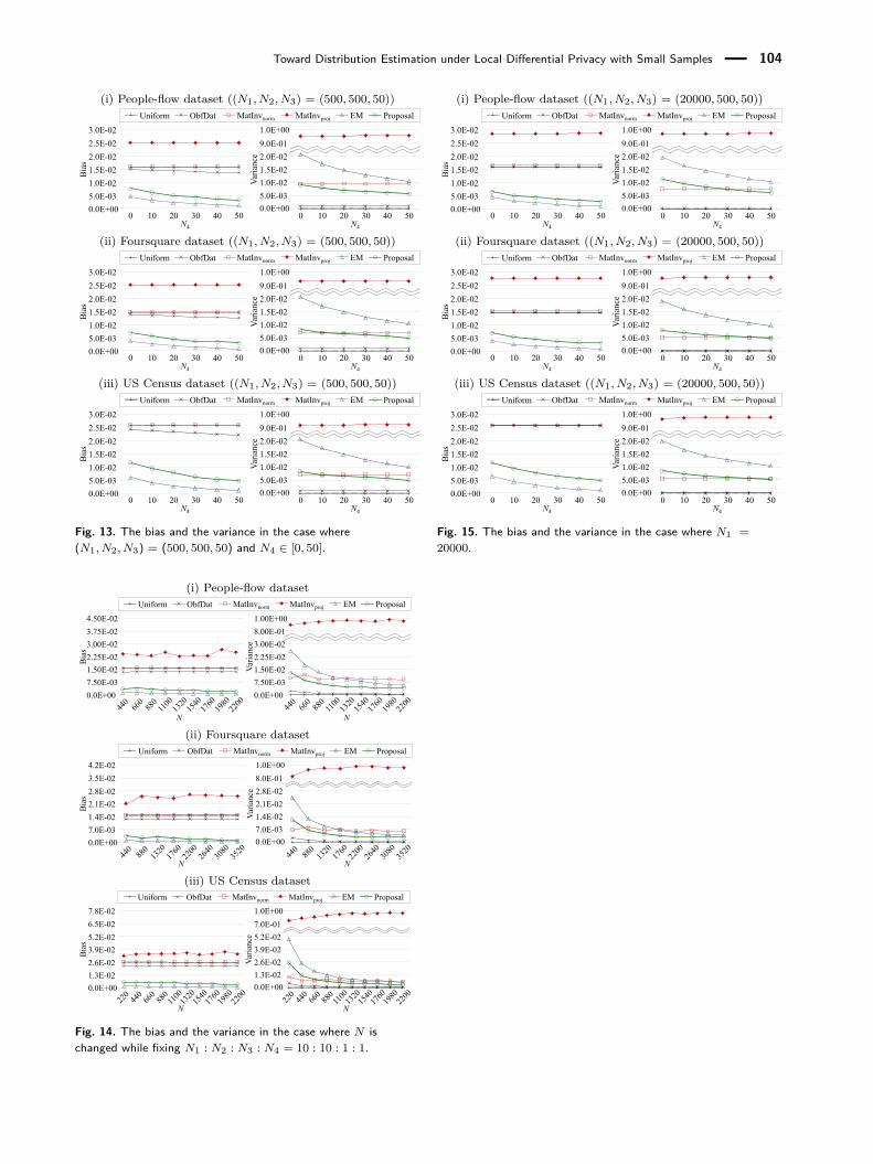
Toward Distribution Estimation under Local Differential Privacy with Small Samples 104
(i) People-flow dataset ((N1, N2, N3) = (500, 500, 50))
0 10 20 30 40 50N4
Uniform ObfDat MatInvnorm EM ProposalMatInvproj
Bia
s
0.0E+005.0E-031.0E-021.5E-022.0E-022.5E-023.0E-02
0 10 20 30 40 50N4
0.0E+005.0E-031.0E-021.5E-022.0E-029.0E-011.0E+00
Varia
nce
(ii) Foursquare dataset ((N1, N2, N3) = (500, 500, 50))
Bia
s
0.0E+005.0E-031.0E-021.5E-022.0E-022.5E-023.0E-02
0 10 20 30 40 50N4
0 10 20 30 40 50N4
0.0E+005.0E-031.0E-021.5E-022.0E-029.0E-011.0E+00
Varia
nce
Uniform ObfDat MatInvnorm EM ProposalMatInvproj
(iii) US Census dataset ((N1, N2, N3) = (500, 500, 50))
Bia
s
0.0E+005.0E-031.0E-021.5E-022.0E-022.5E-023.0E-02
0 10 20 30 40 50N4
0 10 20 30 40 50N4
0.0E+005.0E-031.0E-021.5E-022.0E-029.0E-011.0E+00
Varia
nce
Uniform ObfDat MatInvnorm EM ProposalMatInvproj
Fig. 13. The bias and the variance in the case where(N1, N2, N3) = (500, 500, 50) and N4 ∈ [0, 50].
(i) People-flow dataset
N
Uniform ObfDat MatInvnorm EM ProposalMatInvproj
Bia
s
0.0E+007.50E-031.50E-022.25E-023.00E-023.75E-024.50E-02
N
0.0E+007.50E-031.50E-022.25E-023.00E-028.00E-011.00E+00
Varia
nce
(ii) Foursquare dataset
N
Uniform ObfDat MatInvnorm EM ProposalMatInvproj
Bia
s
0.0E+007.0E-031.4E-022.1E-022.8E-023.5E-024.2E-02
0.0E+007.0E-031.4E-022.1E-022.8E-028.0E-011.0E+00
Varia
nce
N
(iii) US Census dataset
N
Bia
s
0.0E+001.3E-022.6E-023.9E-025.2E-026.5E-027.8E-02
0.0E+001.3E-022.6E-023.9E-025.2E-027.0E-011.0E+00
Varia
nce
N
Uniform ObfDat MatInvnorm EM ProposalMatInvproj
Fig. 14. The bias and the variance in the case where N ischanged while fixing N1 : N2 : N3 : N4 = 10 : 10 : 1 : 1.
(i) People-flow dataset ((N1, N2, N3) = (20000, 500, 50))Uniform ObfDat MatInvnorm EM ProposalMatInvproj
0 10 20 30 40 50N4
Bia
s
0.0E+005.0E-031.0E-021.5E-022.0E-022.5E-023.0E-02
0 10 20 30 40 50N4
0.0E+005.0E-031.0E-021.5E-022.0E-029.0E-011.0E+00
Varia
nce
(ii) Foursquare dataset ((N1, N2, N3) = (20000, 500, 50))Uniform ObfDat MatInvnorm EM ProposalMatInvproj
Bia
s
0.0E+005.0E-031.0E-021.5E-022.0E-022.5E-023.0E-02
0 10 20 30 40 50N4
0 10 20 30 40 50N4
0.0E+005.0E-031.0E-021.5E-022.0E-029.0E-011.0E+00
Varia
nce
(iii) US Census dataset ((N1, N2, N3) = (20000, 500, 50))Uniform ObfDat MatInvnorm EM ProposalMatInvproj
Bia
s
0.0E+005.0E-031.0E-021.5E-022.0E-022.5E-023.0E-02
0 10 20 30 40 50N4
0 10 20 30 40 50N4
0.0E+005.0E-031.0E-021.5E-022.0E-029.0E-011.0E+00
Varia
nce
Fig. 15. The bias and the variance in the case where N1 =20000.