
TAG unit M2 variable demand modelling, March 2017 - gov.uk · 1.2 This TAG Unit 1 ... Assignment...
85
Transcript of TAG unit M2 variable demand modelling, March 2017 - gov.uk · 1.2 This TAG Unit 1 ... Assignment...
Contents
1 Introduction 1
1.1 Background to Variable Demand Modelling 1 1.2 This TAG Unit 1 1.3 Core Requirements 2
2 Scoping the Model and Initial Development 3
2.1 Background 3 2.2 Assessment of the Need for Variable Demand Modelling 3 2.3 Preliminary Assessment of the Scope of the Variable Demand Model 5 2.4 Model Area and Zone Size 7 2.5 Trip Matrices 8 2.6 Segmentation: Trip and Person Types 10 2.7 Division into Time Periods 13
3 Representation of Travel Costs 14
3.1 Generalised Cost Formulation 14 3.2 Composite Costs 16 3.3 Cost Damping 18
4 Model Form and Choice Responses 23
4.1 Background 23 4.2 Functional Form 23 4.3 Form of Models 24 4.4 Model Interfaces 26 4.5 Hierarchy of Choice Responses 28 4.6 Trip Frequency 30 4.7 Mode Choice 30 4.8 Time of Day Choice 33 4.9 Trip Distribution 34 4.10 Route Choice: Assignment Modelling 37
5 Demand Model Calibration 38
5.1 Local Calibration of Demand Models 38 5.2 Trip Frequency 38 5.3 Mode Choice 38 5.4 Time Period Choice 39 5.5 Distribution 39 5.6 Illustrative Parameter Values 40
6 Convergence, Realism and Sensitivity 44
6.1 Background 44 6.2 Building the Model and Model Interfaces 44 6.3 Convergence 45 6.4 Realism Testing 47 6.5 Model Adjustment 52 6.6 Sensitivity Testing 55 6.7 Reporting 56
7 References 57
8 Document Provenance 58
Appendix A Elasticity Models 59

Appendix B An Approach to Building the Base Demand Matrix 62
Appendix C Values of Time for Use with Income Segmentation 64
Appendix D Functional Forms for VDM 66
Appendix E Incremental Model Formulation 71
Appendix F Absolute Model Formulation 75
Appendix G Estimation of Transferred Mode Choice Models 77
Appendix H Use of DIADEM 81

TAG Unit M2 Variable Demand Modelling
Page 1
1 Introduction
1.1 Background to Variable Demand Modelling
1.1.1 Guidance for the Technical Project Manager and TAG Unit M1.1 – Principles of Modelling and Forecasting explain why variable demand modelling needs to be considered in a scheme appraisal. The technical project manager guidance explains how to establish whether there is a need for variable demand modelling in a particular application. Assuming that there is a need, it then goes on to give preliminary advice on the scope of the model, with a view to developing a model which is appropriate for the complexity of the interventions that it will be used to test.
1.1.2 Any change to transport conditions will, in principle, cause a change in demand. The purpose of variable demand modelling is to predict and quantify these changes.
1.1.3 It is of key importance in modelling to establish a realistic scenario in the absence of and with the inclusion of the proposed scheme or strategy. For schemes that may affect traveller behaviour such as choice of mode, realistic levels of demand across the modes needs to be established.
1.1.4 Although the modelling effort needs to be proportionate to the scale of a potential intervention, the need to consider variable demand is not simply a question of the size of the intervention. Since both demand changes and benefits tend to scale with the size of the scheme, changes in demand can have similar proportionate effects on benefits for both large and small schemes. Thus changes in demand can have fundamental implications for the justification of a scheme of any size, in terms of economic, environmental and social impacts and should be represented appropriately and proportionately.
1.1.5 Any response in the demand for transport of freight is not considered here, since it is often sufficient to assume that total freight traffic is fixed, but susceptible to re-routeing. See TAG Unit M1.1, Section 4.3, for further details.
1.2 This TAG Unit
1.2.1 This TAG Unit describes the considerations and processes required in variable demand modelling:
• Scoping out the requirements of the model, based on the objectives at hand and the requirements of a fit-for-purpose forecasting tool, including scoping the need for having a variable demand model at all by testing how important including demand responses might be and whether it is acceptable to exclude them (Section 2);
• Formulation of how travel costs (disutilities) will be handled within the model (Section 3);
• Development of the model and appreciation of the model form and choice responses that need to be represented (Section 4);
• Ensuring that the model is appropriately calibrated using local data sources or illustrative model parameters (Section 5);
• Ensuring that the model is valid and fit-for-purpose, by ensuring convergence, undertaking realism tests and running sensitivity tests around key parameters (Section 6).
1.2.2 Throughout the advice there are a number of important recommendations shown highlighted and in bold: if these actions are not followed, analysts will need to provide rigorous justification for the course of action taken.

TAG Unit M2 Variable Demand Modelling
Page 2
1.3 Core Requirements
1.3.1 The intention of this advice is to describe the basis of variable demand modelling as clearly and simply as possible and it is intended to represent generally-accepted best practice. A summary of the main points to note regarding core requirements is as follows:
• Overall, there should be a presumption that the effects of variable demand on scheme benefits will be estimated quantitatively unless there is a compelling reason for not doing so. This may be justified by undertaking scoping tests as described in Section 2.2. The justification for the approach adopted, including the results of these tests where conducted, should be reported in an Appraisal Specification Report. Even if induced traffic does not alter the case for the scheme appreciably, the assessment may be criticised if it cannot demonstrate that the case is robust against possible changes in demand.
• The amount of detail required in demand modelling will depend upon the particular application, since the effort and cost involved should be commensurate with the investment being assessed and the scale of its effects. A distribution mechanism is expected to be included where discrete choice models are used.
• In modelling demand, some segmentation by trip and traveller type is essential: at minimum there should be categorisation by trip purpose (at least home-based work (commuting), employer’s business, and ‘other’ purposes); some form of distinction between travellers with and without a car available is also very desirable and is expected where mode-choice is to be considered. In many cases, modelling multi-car ownership is desirable, and should be practicable, if household survey data sets are available or sufficient data are available for its synthesis.
• The sequence of the distribution and mode split stages in the calculation hierarchy depends upon the relative strengths of the sensitivity parameters, but trip frequency should always be calculated first (highest) and micro time period choice (peak-spreading), if it is to be included, will generally be lowest in the demand model hierarchy, with route choice (within the assignment model) being the most sensitive. The sensitivity parameters must always increase (strictly never decrease) along this sequence from highest to lowest, and this may require different sequences for different segments of travel (e.g. purpose, etc.). In the absence of strong evidence to the contrary, the model should adopt the default hierarchy of responses as recommended in Section 4.5.
• All transport models depend upon relating people’s travel choices to estimates of their generalised cost of travel – a weighted sum of time and other costs of travel which can be measured in units of money or (preferably) time; these costs are estimated within both the demand model and assignment model.
• The Department’s long-established preferred approach is to use an incremental rather than an absolute model, unless there are strong reasons for not doing so.
• Convergence between the assignment and the demand model(s) is very important and must be clearly reported.
• Variable demand mechanisms should be calibrated on local data, to reflect the local strengths of the choice mechanisms, or where this is not possible; the illustrative parameter values presented in this unit may be used, obtained from a review of UK transport models.
• It is essential to apply realism testing to ensure that the model responds rationally and with acceptable elasticities.
• It is also necessary to apply sensitivity testing to determine the variation in the results of the assessment against the uncertainty in the input parameters.

TAG Unit M2 Variable Demand Modelling
Page 3
2 Scoping the Model and Initial Development
2.1 Background
2.1.1 This Section describes some of the early choices that need to be made when considering the development of a variable demand model. This includes preliminary tests for the need of such a model and, once a need is ascertained, defining the scope of the model in general. The following Sections go into more detail regarding specific components of the demand model and the calibration process.
2.1.2 This guidance is based on cases where a full multi-modal model with appropriate segmentation and representation of demand responses is required. Less detail may be acceptable, though it will be expected that an appropriate case is made at an early stage for any simplifications adopted (see Guidance for the Technical Project Manager and the requirements for an Appraisal Specification Report). In particular, readers should consult Section 2.3 regarding the need for a full representation of alternative modes.
2.1.3 A summary of the advice in this Section is as follows:
• An initial assessment of the need for a variable demand model should be undertaken. This is discussed in Section 2.2.
• Once the need for a variable demand model has been established, some initial decisions concerning the basic structure of the model are required. These should be based on the expected transport problems and likely solutions being assessed. This is discussed in Section 2.3.
• The demand and supply processes need to allow for trip redistribution when designing the zone system and provide a fine enough level of detail for the schemes and strategies being assessed. This is discussed in Section 2.4.
• Various stages of the demand modelling and forecasting process require travel movements to be described in terms of the factors that generate or attract trips – i.e. by productions and attractions (P/A). Section 2.5 discusses the conversion between P/A and origin/destination (O/D) forms for use in the multi-stage modelling process. It also discusses the requirement to construct a base year travel pattern and reference case growth forecasts.
• The impacts of different policy measures on particular groups of people can only be represented realistically and forecast satisfactorily if the demand modelling process is suitably segmented. Modelling should use groups of travellers (segments) that it is expected will continue to behave in similar fashion over time. This is discussed in Section 2.6.
• Travel demand and traffic levels vary throughout the day and this usually requires the modelling of different time periods. The need to divide the day into different periods, related to the daily profiles of road traffic, is no more onerous than is normally needed in assignment modelling, unless it is intended to model peak spreading, as described in Section 2.7.
2.2 Assessment of the Need for Variable Demand Modelling
2.2.1 It may be acceptable to limit the assessment of a scheme to a fixed demand assessment if the following criteria are satisfied:
• The scheme is quite modest either spatially or financially and is also quite modest in terms of its effect on travel costs. Schemes with a capital cost of less than £5 million can generally be considered as modest; or the following two points:

TAG Unit M2 Variable Demand Modelling
Page 4
• There is no congestion or crowding on the network in the forecast year (10 to 15 years after opening), in the absence of the scheme; and
• The scheme will have no appreciable effect on travel choices (e.g. mode choice or distribution) in the corridor(s) containing the scheme.
2.2.2 Under congested conditions, the without-scheme forecasts may be affected by peak spreading (change in micro-time period choice), or diverted or suppressed traffic. It will often be the case that such suppression will have a greater impact on the scheme benefits than any induced traffic from the scheme itself. It is, however, expected that where a variable demand model is used for forecasting, then that model will be used to derive forecasts for all scenarios, both with and without the scheme.
2.2.3 The benefit from schemes can be substantially altered by changes in demand arising from the scheme. Any scheme potentially encourages more use of the transport network and hence may affect congestion levels - in the case of highway schemes over the entire journey distances travelled by the traffic through it. Even where congestion is minimal under the expected operating conditions and induced traffic may have little effect on speeds on the scheme, there may still be substantial reductions in speeds on roads leading to and from it due to induced traffic. Those extra induced trips and longer trips are the key components of induced traffic.
2.2.4 In order to establish a case for omitting variable demand in the model, preliminary quantitative estimates of the potential effects of variable demand on both traffic levels and benefits should be made.
2.2.5 An existing variable demand model of the area should be used for the purpose of testing if one is available, Otherwise, since a highway assignment model is usually a minimum requirement for scheme appraisal, an elastic assignment procedure can be used to give an initial indication of the effects of variable demand. The limitations and uncertainties surrounding such an approach must be appreciated, and further evidence must be collected in order to determine that inclusion of variable demand is not necessary. A key indicator is often the level of cost change that is expected in the future or due to an intervention. Where this is likely to be significant, as suggested by the indicative tolerances below, some form of variable demand model will be a requirement.
2.2.6 Where preliminary calculations using an existing variable demand model are carried out, it will be acceptable in general to use a fixed demand assessment where the resulting difference in suppressed/induced traffic when using the demand model does not change benefits resulting from a scheme by more than 10% in the opening year and 15% in the forecast year (10 to 15 years later) relative to a fixed demand case.
2.2.7 These calculations may provide strong enough evidence to conclude that the impact of variable demand will be negligible and thus provide a useful justification for restricting the assessment to fixed trip matrix. However, the possible superiority of alternative schemes that may have more significant impacts on demand, including potential improvements to public transport, also needs to be considered.
2.2.8 If it is decided that variable demand modelling is required then the scope of the variable demand model must be established. See Section 2.3.
2.2.9 The outcome of the assessment of the need for a variable demand model, as well as the series of tests outlined below, should be reported in the Appraisal Specification Report (see Guidance for the Technical Project Manager). Details of how each criterion has been considered and all the evidence that has been compiled should be fully documented. In all cases, the analyst will need to provide a justification for any simplifications adopted.

TAG Unit M2 Variable Demand Modelling
Page 5
The Status of Elasticity Methods
2.2.10 “Own-cost” elasticity models assume that the demand for travel between two points is purely a function of the change in costs on that mode between the two places. The strength of that function can vary for different trip lengths.
2.2.11 It is recommended that own cost elasticity models are not used instead of full variable demand models1. An own cost elasticity model applied to all trips cannot recreate the change in pattern of travel nor all of the changes in trip lengths that are forecast by a trip distribution model, nor can it properly represent the transfer of trips from one mode to another when there are changes to the cost of several modes or the transfer from one time period to another. Research has shown that elasticity models may significantly overestimate the effect of variable demand responses on scheme benefits.
2.2.12 There may be a role for elasticity models in option testing to proxy full variable demand model results where it would be disproportionate to run the full model. This may be particularly useful if the model takes a long time to run or there are a large number of potential options. However, the analyst must note the caveats related to elasticity-based methods and be satisfied that the results do not mislead in order to avoid poor options being taken through to the full modelling stage. If an elasticity approach is to be applied in this way, then Appendix A sets out the different possible formulations.
2.3 Preliminary Assessment of the Scope of the Variable Demand Model
2.3.1 Having concluded that a variable demand model is required, it is necessary to take a view on the scope of the modelling system. TAG Unit M1.1 – Principles of Modelling and Forecasting describes the stages required in a full model system, including the role of the demand model and its interaction with assignment.
2.3.2 The analyst should explore whether or not a potentially suitable model of the required area already exists in order to apply it to the transport problem and proposed solutions. Such a model may require adjustment to this particular case, but may substantially save time in development. However, where there is no existing model, the analyst must ensure that the effort in constructing a model to appraise an intervention is proportionate.
2.3.3 Typically, the demand model should address the responses of frequency, mode choice and destination choice, as well as, in some instances, time of day, and should be applied on a Production/Attraction [P/A] basis. However, while for large and complex schemes a full variable demand approach is likely to be required, not all schemes will require this, and it is important that the model is appropriate for the interventions that it will be used to test.
2.3.4 For the majority of cases, it will be essential to model AM peak, PM peak and inter-peak time periods. The modelling of off-peak periods (before the AM peak and after the PM peak) may be worthwhile where important impacts occur in this period (e.g. noise or air quality issues).
2.3.5 The main possibility for simplification relates to the treatment of mode, since much of the modelling effort can be attributed to measuring the impact on alternative modes. If it is the case that the model is required to appraise policies relating to both highway and public transport modes, it will be unlikely that any simplification in the level of modal detail from a fully-specified approach can be made. However, when policies relate only to one mode, it may be possible to concentrate on that mode.
2.3.6 Where there is limited scope for transfer between modes, the demand model may not require a mode choice element nor the representation of the costs of alternative modes in any detail (and
1 A common exception is in rail appraisals, which often make use of elasticity-based demand forecasting methods (using elasticities from the Passenger Demand Forecasting Handbook (PDFH)). These models are often uni-modal rather than multi-modal, commonly lacking explicit representation of other modes.

TAG Unit M2 Variable Demand Modelling
Page 6
hence may not need an associated assignment model for those modes). Simplifications of this kind are likely to also impact on the level of detail required in the demand model. For example, in the case of a highway scheme where no shift to or from public transport is expected, the demand model segmentation may be restricted to car users only.
2.3.7 There may also be scope for simplification in the supply model where there may not be significant routeing alternatives. In a public transport scheme where crowding is a possibility, the generalised costs are dependent on the level of demand and more detailed representation, most likely involving a public transport assignment model, is warranted. However, when crowding is not present, and route choice is simple (because of restricted alternatives), the need for a public transport assignment model is greatly reduced. This applies even in the case of a policy relating to public transport.
Modal Shift Significance Test
2.3.8 In principle, any change in relative generalised cost between the modes will lead to some modal shift. However, this sensitivity is usually low, as implied by the mode choice parameters in Section 5.6. A test can been formulated to make a preliminary estimate of the likely amount of modal diversion, as follows:
• For each zone-to-zone movement, using available data, estimate the approximate modal split between car and public transport, and the change in costs expected to arise from the scheme for each mode.
• The modal impact may be considered significant if, for any zone to zone movement where the car share is below 75%, the cost change between modes is more than one minute, or, where the car share is between 75% and 85%, the cost change is more than two minutes, or, where the car share is above 85%, the cost change is more than four minutes.
• If on this basis no zone-to-zone movement demonstrates significant modal impact, then this is prima facie evidence for not requiring a mode choice model.
Logical Tests for Provisional Model Scope
2.3.9 A set of logical tests has been defined to give a clear assessment of which modes need to be modelled:
• Test 1 - Do the set of schemes to be appraised relate to only one of the modes; public transport and highway? If NO, a multi-modal treatment will, in principle, be required.
• Test 2 - If the scheme is highway only, does the application of the mode shift test suggest that there will be a significant impact on public transport demand? If YES, a mode choice model will, in principle, be required.
• Test 3 - If the scheme is public transport only, does the application of the mode shift test suggest that there will be a significant impact on highway demand? If YES, a mode choice model will, in principle, be required.
• Test 4 - If the scheme is highway only, and a mode choice model is not required, then a public transport assignment model is not required.
• Test 5 - If the scheme is public transport only, and a mode choice model is not required, then a highway assignment model is not required. In addition, a public transport network model may not be necessary if the level of crowding is not expected to be significant during the lifetime of the scheme, and routeing is generally straightforward.
• Test 6 - If the scheme is public transport only, then, even if a mode choice model is required, it may be proportional to manage without a highway assignment model and use the techniques

TAG Unit M2 Variable Demand Modelling
Page 7
described in TAG Unit A5.4 – Marginal External Costs to measure decongestion benefits (through use of “Marginal External Costs of Congestion”). This will only be appropriate where there is no impact from the scheme on highway capacity, the analyst is satisfied that highway costs are adequately represented in the base and forecast years where a mode choice model is in use and there is a relatively small amount of mode shift (i.e. the highway costs are not anticipated to change significantly). In addition, as in Test (5), a public transport assignment model may not be necessary if the level of crowding is not expected to be significant during the lifetime of the scheme, and routeing is generally straightforward.
Mode Choice Model: Bespoke or Transferred?
2.3.10 In practice, where a mode choice model is a requirement, the majority of model developers transfer the mode choice component from other similar model types and structures. Bespoke models may occasionally be required in cases where appropriate models to transfer do not exist or are of insufficient quality, or the scope of the model or scheme is sufficiently large and complex to warrant such an approach. An example of this is where a new mode is required to be modelled, for very large public transport schemes, or where traveller behaviour, e.g. in terms of values of time, is substantially different from national norms.
2.3.11 Many models may fall somewhere between pure ‘bespoke’ and ‘transferred’ types, depending on how the ‘imported parameters’ are obtained, and the extent to which local data is available to calibrate the model. As part of the calibration procedure, it is important that the model sensitivities are replicated (and in the case of absolute models, the observed mode shares).
2.3.12 Further information on construction of bespoke mode choice models can be found in the Supplementary Guidance section of WebTAG. Section 4.7 provides some guidance on how to estimate mode choice models in the context of transferred models.
Land Use and Transport Interactions
2.3.13 Undertaking a land use transport interaction model is costly, data-hungry and time-consuming. For some cases, however, the impact of the scheme on regeneration is expected to be substantial and therefore an important part of scheme appraisal. In these cases, this option should be carefully considered.
2.3.14 Where such expenditure is not defensible, an alternative approach is to extract measures of accessibility from the transport model and use these to inform expert judgement. In cases where an objective of the scheme is simply to improve accessibility these measures are in principle sufficient in themselves, but they can also give sufficient information for an expert to assess what land use changes are likely.
2.4 Model Area and Zone Size
Model Area
2.4.1 The consideration of the spatial area to be represented by both demand and assignment models is a balance between the area being large enough to capture all the salient impacts of a scheme, whilst not being so large that model runtimes, convergence and noise become a problem (TAG Unit M1.1 has more details). The overall maxim is that the model area should be fit for purpose in order to fully account for not only the route choice impacts, but the choices on the demand side as well.
2.4.2 TAG Unit M3.1 – Highway Assignment Modelling and TAG Unit M3.2 – Public Transport Assignment Modelling, give guidance on defining an appropriate modelled area for assignment models. This will usually be composed of an Area of Detailed Modelling, in which both routeing and demand responses are expected to occur and hence it is desirable to have the representation of the network and zoning system as detailed as possible. The rest of the fully modelled area may contain larger zones and less network detail. The external area will usually consist of very large zones and a skeletal network. The “study area” would generally equate to the fully modelled area.
TAG Unit M2 Variable Demand Modelling
Page 8
2.4.3 Movements between the internal and external areas need to be represented at an appropriate level of detail, for four reasons:
• On the demand side if only internal movements are properly represented as trips, then zones near the border will have (apparently) lower levels of trip-making.
• When modelling destination choice, travel opportunities to both internal and external zones need to be represented. Thus, although the external area can be represented at a coarse geographical level, it is important that it should contain sufficient close destinations, and appropriately attractive ones, to take a realistic share of demand from within the modelled area.
• Similarly, zones just outside the fully modelled area need to provide a realistic demand into the area. Hence, the fully modelled area should be surrounded by a ring of ‘buffer’ zones with a dimension a little larger than the internal zones, and outside these will be very large zones representing the rest of the external area.
• On the supply side, movements from one external zone to another external zone may form ‘through traffic’ in the modelled area and this may respond to factors beyond the scope of the model.
Zone Size and Intrazonals
2.4.4 The size of internal zones will need to be carefully considered in relation to intrazonal trips in order to avoid any biases in the demand model. At the distribution stage it is important to be able to redistribute intrazonals to become interzonals, and interzonals to become intrazonals, if relative costs change. If the zone sizes are small this is less of a problem, but for large zones it is important that the average intrazonal costs are as realistic as possible.
2.4.5 Various approaches may be used to derive intrazonal costs:
• assume the average cost of an intrazonal trip is a fixed proportion of the costs of interzonal trips to the neighbouring zones, or
• assume the mean distance of an intrazonal trip is a proportion of distance to the neighbours and costs generated accordingly.
2.4.6 Intrazonal costs should reflect the prevailing level of congestion via the mean journey speeds, and preferably its response to changing demand. Basing costs on those of trips to the neighbouring zones will generally be sufficient.
2.4.7 As noted in TAG Unit M3.1, cordon models are not recommended, since they do not allow a full representation of end-to-end costs for journeys crossing the cordon. The use of truncated costs will render some forms of demand model inappropriate whereas the use of end-to-end journey costs will allow the modeller greater freedom in the choice of demand model.
2.5 Trip Matrices
Matrix Form
2.5.1 The majority of contemporary models use trip-based matrices. In a number of transport models, however, the modelling is not based on trips but on tours. A “tour” is defined as any round trip, starting and finishing at home, and may contain stops at several different destinations. Journeys between non-home destinations are handled automatically in these models, but most demand models treat them as Non-Home Based trips. A choice can be made by the model developers between trip-based and tour-based approaches. In general, a tour-based approach can be considered to give higher quality representation of behaviour in several of the components of the

TAG Unit M2 Variable Demand Modelling
Page 9
model system2, but they are, at the present time, generally restricted to large scale strategic models. If available, they could be used to provide inputs to more locally based models.
2.5.2 Where a non-uniform growth is forecast at either the production (home) end or the attraction end, forecasts produced using O/D matrices will be less accurate than those produced using P/A based matrices. For this reason P/A matrices should be used, even if no explicit trip distribution modelling is performed.
2.5.3 There are a number of circumstances, however, where it may be satisfactory to use O/D based matrices for forecasting, largely for reasons of practicality. This may be where the model is simple enough or used for a specific enough purpose that the analyst can be confident that the forecasts will not be biased, such as where forecasts are based on a simple overall growth rate, or only the AM peak is being modelled, etc. This situation is expected to be very uncommon. Advice should be sought from the Department before specifying the model if this approach is being considered.
Matrix Building
2.5.4 TAG Unit M1.2 – Data Sources and Surveys gives guidance on data sources that are appropriate to construct and calibrate demand models. The data required for the demand calculations depend upon the chosen level of segmentation (i.e. disaggregation) of travellers and travel characteristics, as discussed in Section 2.6.
2.5.5 There are two separate processes that need to be considered when developing forecast matrices for use in demand models:
• the production of a base year travel pattern (replicating observed movements and behaviours in the base year), and
• the production of reference cases for future years (estimating future travel demand based on demographic changes, prior to consideration of changes in costs).
Deriving the Base Year Travel Pattern
2.5.6 As discussed, variable demand models require base year matrices in Production/Attraction (P/A) form. The method of constructing these matrices is dictated by the modelling approach, but in most cases is expected to be an all-day (or 16 / 12 hour period) model, see Section 2.7. As advised in Section 4.3, however, unless there are compelling reasons to the contrary, the Department’s strong suggestion is to use an incremental approach, either using a pivot-point model or based on incremental application of absolute estimates.
2.5.7 This Section discusses the construction of a base year matrix based on observed and synthesised data to form a calibrated base situation for an incremental model. The same data will be used in order to calibrate the demand responses of an absolute model. For further detail on model forms, see Section 4.3.
2.5.8 The base P/A matrix can be constructed from observed travel movements based on road-side and passenger surveys, as well as household survey data. In theory it should also be possible to make use of traffic counts; the fact that these contain no associated directional or purpose information means that methodologies for doing this are only recently being developed. Opportunities for exploiting technologies such as GPS devices and mobile phone data could be explored, although these may encounter similar problems and the potential bias in these sources should be thoroughly understood.
2.5.9 The detail available in these travel patterns is largely dictated by the richness of the survey data. In reality the procedure to provide the “best” base matrices will always involve some synthesis as not all movements will be surveyed. In carrying out a synthesis of a P/A matrix, it will generally be
2 Examples include use where parking or time-specific charging systems are a key consideration.

TAG Unit M2 Variable Demand Modelling
Page 10
desirable to base the productions on some reputable trip end model and data from the National Trip End Model (NTEM), provided in the TEMPRO software, should be treated as the default in this respect. Alternatively, more detailed local data may be available to use with the model, but it will be necessary to ensure that at a broad level it is consistent with the assumptions of the NTEM data.
2.5.10 Matrix building is a complex topic, where several different approaches have been used in the development of models. The Department recognises the need to develop more guidance in this area. In the interim, Appendix B contains one approach that could be adopted. Whichever approach is used, it is important that the approach adopted is identified early and thoroughly explained in the Appraisal Specification Report.
Production of Reference Cases for Future Years
2.5.11 Modelling of incremental changes from the base matrix is required for most assessments. For very large schemes or situations where there will be substantial land-use and demographic changes within the timescale of the assessment, however, it may be necessary to make a detailed absolute forecast of at least part of the future reference case (see Section 4).
2.5.12 The construction of the reference case forecast requires reference case growth factors/assumptions and will involve the adjustment of the row and column of the base P/A matrix at an all-day all-modes level to reflect expected land-use and car ownership changes (taking no account of cost changes). As a default, these should be based on NTEM.
2.5.13 If the O/D matrix is made incompatible with the P/A matrix, i.e. by means of matrix estimation, it will often be necessary to undertake an incremental assignment, adjusting the validated base year matrix based on the incremental output from the demand model (however, again, other emergent methods may be available).
2.5.14 During the modelling process, trip matrices must be converted from a P/A basis to an O/D basis. This is discussed in Section 4.4.
2.6 Segmentation: Trip and Person Types
2.6.1 “Segmentation” is the division of travel, traveller and transport attributes into different categories so that all travellers in the same category can be treated in the same way.
2.6.2 In general, assignment and demand models require different forms of segmentation. Demand modelling generally requires more categorisation, both in order to estimate how much demand, and of what type, a particular zone may produce or attract, and because different types of traveller respond differently to changes in travel conditions and costs.
2.6.3 To be accepted by the policy-makers, forecasting and assessment must be seen to deal realistically with the variety of external factors which will contribute to changes in travel demand. Moreover, policy makers may wish to know whether policies impact differently on different types of traveller, and if so, how. However, segmentation increases the size, complexity and run times of models, as does a more detailed spatial description using smaller zones, and judgements have to be made about how much detail is necessary in a particular application. The same degree of segmentation may not be necessary at all stages of the model, and each of the stages of the demand model is considered in turn in the detailed discussion below.
2.6.4 Ultimately the segmentation adopted in the modelling process must depend on the nature of the study area, the objectives of the study, the data available, the outputs required and the intended model structure. Table 2.1 suggests the minimum levels of segmentation for demand modelling. Note that these are guidelines on minimum segmentation, they are not necessarily adequate, and the degree of segmentation used should depend upon the particular application and the resources available.

TAG Unit M2 Variable Demand Modelling
Page 11
Table 2.1 Minimum Segmentations for a Multi-Stage Demand Model Attribute Segmentation Household type and traveller type
Two categories: travellers categorised into car-available/no-car-available or by household car ownership into car-owning/non-car-owning. Models that only need to deal with road traffic will include only those travellers who have a car available. If a local trip generation model is being developed, a more detailed segmentation into household structure, employed members, etc is very desirable and used in NTEM, but this finer level of segmentation need not be carried through to the subsequent stages.
Value of time Variation of VOT across the population is important but can usually be addressed sufficiently through the trip purpose split. However, for schemes specifically involving charging, some additional segmentation by willingness-to-pay or income may be required. In this case 3 separate income ranges – high, medium and low (with different VOT) with demand distributed evenly across the groups - will be adequate (see Appendix C). Where there is a large range of trip distance, it is desirable to allow VOT to vary with trip distance (see Section 3.3).
Trip purpose 3 categories: Commuting/ Employer’s business/ Other: these categories are likely to have different elasticities and different distributions in both time and space, and substantially different values of time.
Modes 2 categories: Car/public transport. It is usually necessary to have a base of trips that can transfer to and from car.
Road vehicle types
2 categories: Car/other, where the “other” may include freight and bus/coach as a fixed-flow matrix for assignment.
2.6.5 While it is undoubtedly useful to use a more elaborate segmentation of the population at the trip
generation stage in order to facilitate forecasting, there is generally less requirement to carry such segmentation forward into subsequent stages of the model. A distinction between purposes is however essential; a suitable starting point would be – commuting, employer’s business and others. Currently values of time used in appraisal are considered different for these purposes (see the TAG Data Book). Where mode choice is modelled, it will also be important to make a distinction between travellers who have a car available for a trip and those who do not and are therefore limited in their choice of modes.
2.6.6 Not all stages of the demand model require the same degree of segmentation. The guidance below gives more detail on what is needed for each stage, and considers the associated value of time issues.
Trip Frequency
2.6.7 For most purposes it will be satisfactory to take the observed trip pattern and modify this pattern incrementally by making it respond to changes in travel times and costs. Categorisation by trip purpose (where the values of time are assumed to differ) is usually more than sufficient. It is also possible to assume that only certain trip purposes will change their frequency in response to changing travel costs, for instance trip frequency changes may be modelled for leisure trips but not for commuting trips.
Trip Distribution
2.6.8 The distribution model estimates the number of trips between each pair of zones, and ideally includes intrazonal trips which begin and end in the same zone, as well as the interzonal trips. It should be noted that it may be necessary to apply area-specific constants or movement-specific deterrence functions within the distribution model to reflect the difference in the nature of travel to

TAG Unit M2 Variable Demand Modelling
Page 12
certain areas (e.g. longer distance trips to city centres). If this particular problem arises for the application being considered, some form of income or socio-economic group (SEG) segmentation may be appropriate to reflect how, for example, jobs in city-centres may have a high component of high SEGs such as professional and managerial posts in finance, banking and other business services, where workers may be drawn from further away producing higher average trip distances. A similar pattern may emerge for shopping trips to the city centre and both may require a white collar /blue collar distinction, for example at a zonal trip attraction level. However, for most applications such a complication will be unnecessary.
Mode Choice
2.6.9 Since the choice of mode depends on whether a traveller has a car available for the journey it is desirable to categorise travellers according to car availability for the trip, but since this is hard to identify in practice the segmentation is often merely available or non-available with more detail being by the level of household car ownership such as 0, 1 or 2+ cars. The model must include all relevant modes between which to choose, although will often omit active modes (walk and cycle). It is standard practice to develop models with different parameter values for different purposes and different categories of car availability.
Time of Day Choice
2.6.10 Where time of day choice is modelled explicitly this choice mechanism can represent either macro time period choice (the broad choice between time periods, e.g. 2 to 3 hours in length) or micro time period choice (choice of travel time within a ‘macro’ period, e.g. between hourly or 15 minute slices). The definition of the modelled time periods should be consistent with the choices to be made and the necessary segmentation by trip purpose, since obligatory travel such as work and education is likely to have less flexibility in adjusting its time of travel than travel for more optional purposes such as shopping or leisure.
Value of Time
2.6.11 Different user classes will have a different willingness to trade money for time in order to visit their destinations. The demand model should be suitably segmented in order to reflect the differences in the values of time between groups. See Section 3 and Appendix C for details.
Public Transport Considerations
2.6.12 An important influence on the use of public transport by those with a car available is whether or not they also have access to a convenient parking space. Consideration should therefore be given to segmenting the home-based work demand by the availability of a parking space at the workplace. For further details on the requirements of modelling where parking is a key consideration, see TAG Unit M5.1 – Modelling Parking and Park-and-Ride.
2.6.13 Segmentation of demand according to the type of ticket or fare concession may also offer a significant improvement in model accuracy. For instance, many senior citizens, children and students are able to take advantage of fare concessions and may travel more than they would if they did not have the concessions. Consideration should therefore be given to the extent to which demand should be segmented by these groups.
2.6.14 Travellers using a public transport link to an airport have special characteristics which need to be reflected in the model. First, the distinction must be made between air passengers and airport workers. The propensity of air passengers to use public transport to access the airport depends strongly on whether they are travelling on business or leisure and whether they are in the home area or away from home. The use that airport workers can make of a public transport service is limited by the availability of services which fit in with their shift patterns.
TAG Unit M2 Variable Demand Modelling
Page 13
2.7 Division into Time Periods
2.7.1 Travel conditions vary considerably across the day, and across the days of the week and time of year. Models usually represent a weekday during a ‘neutral’ or representative month. In order to capture the variation in conditions within the modelled day, and especially the fact that many schemes are aimed primarily at times of maximum travel demand and highway congestion, it is conventional practice to divide the day into different periods for modelling purposes.
2.7.2 A judgement must be made as to how best to define the time periods so that, within each, travel conditions are sufficiently constant to provide a realistic mean cost for the modelling purposes. A balance needs to be struck between the level of detail in the assignment model and the need for detail elsewhere in the modelling process (the number of time periods, the level of detail in the various segmentations, the stages included in the demand model, etc).
2.7.3 In general, demand modelling uses relatively broad time periods. When examining times and places of high congestion, it may be desirable to introduce a higher level of time-dependent responsiveness into assignment, either by modelling a series of short time-periods, or by dynamic assignment which represents explicitly the variation of demand over time, in order to obtain a better estimate of these average costs.
2.7.4 Demand modelling depends upon the time-divisions of the traffic assignment because the relevant travel costs and journey times which are extracted from the assignment are averages across the assignment periods. Hence, it is important to ensure consistency between the time-periods used in the calculation of these averages and the key time periods for the main demand segments.
2.7.5 However, the demand modelling can be assumed to take place over different time-periods, such as 24 hour weekday or 16 hours. In theory, different demand responses can be modelled over different time-scales. A good deal of the survey data will be collected over a 12 hour or 16 hour period, and the background changes in trips estimated from NTEM data are on a 24 hour basis. Many of the current large regional models estimate trip frequency, mode choice and distribution over a 24 hour time period. However, procedures need to be adopted to convert such 24 hour trip patterns to be compatible with the shorter time-scales generally required for assignment modelling (a peak hour or an average inter-peak period, for instance).
2.7.6 Guidance on division of the modelled period into time periods and time slices is given in Traffic Appraisal in Urban Areas DMRB 12.2.1. It recommends that automated traffic counts should be used to establish a daily profile across at least a week’s traffic data, and that subdivision should only be made where there is a clear difference in traffic congestion and/or travel patterns, or where there is an intention to model time of day choice. However, if modal transfer between private and public transport is important, and public transport offers different fares or frequencies at different times of day, it is advisable to choose time periods to reflect their different costs.
2.7.7 TAG Unit M3.1 – Highway Assignment Modelling discusses the development of appropriate time period models in detail. It is unlikely that inclusion of variable demand modelling will require any greater segmentation of time periods than is satisfactory for assignment, except where there is an interest in modelling time of day choice, as discussed in Section 4.8.
TAG Unit M2 Variable Demand Modelling
Page 14
3 Representation of Travel Costs
3.1 Generalised Cost Formulation
3.1.1 All transport modelling should recognise that people’s travel choices depend upon the cost, in both time and money. It is important to combine time and money into a single disincentive to travel (“disutility”), so that demand can be assumed to rise or fall with reductions or increases in either. To do so, it is necessary to apply appropriate weights to the time and money components of this combined cost so that travellers can trade money for time, such as in choosing between a faster but more expensive mode or a slower but cheaper mode.
Components of generalised cost
3.1.2 Two kinds of variable can enter into the function of generalised cost:
• variables which relate to the trip under consideration, and
• variables which relate to the individual making the choice.
3.1.3 Taking mode choice as an example, the cost function developed for the choice of, say, rail by an individual can be influenced both by variables relating to rail (e.g. travel time, fare) and by variables relating to the individual (e.g. income, gender, journey purpose). In principle the generalised cost structure permits a considerable level of variation in behaviour to be examined and allowed for in the forecasting process.
3.1.4 Different groups of people will trade off time and money in different ways: for example, company car owners may be less affected by rises in fuel prices, and holders of certain kinds of public transport tickets may receive free marginal travel. There is likely to be further variation by trip purpose and time of day, which can be modelled using segmentation or disaggregation.
3.1.5 Each segment considered will have, in principle, different parameters in the generalised cost function. Central to this is the concept of value of time (VOT), whereby money costs are converted into time units or vice-versa. Different values of time are appropriate to different segments of the travel market, particularly according to different journey purposes. It is usually sufficient to use the mean VOT across a user segment. Where some form of charging is central to the scenarios being tested, it will be important to include income group segmentation explicitly; in this case the analyst will be required to set the appropriate average value of time for each group, separated by purpose. Further information on this is given in Appendix C, with more on values of time in general in TAG Unit A1.1.
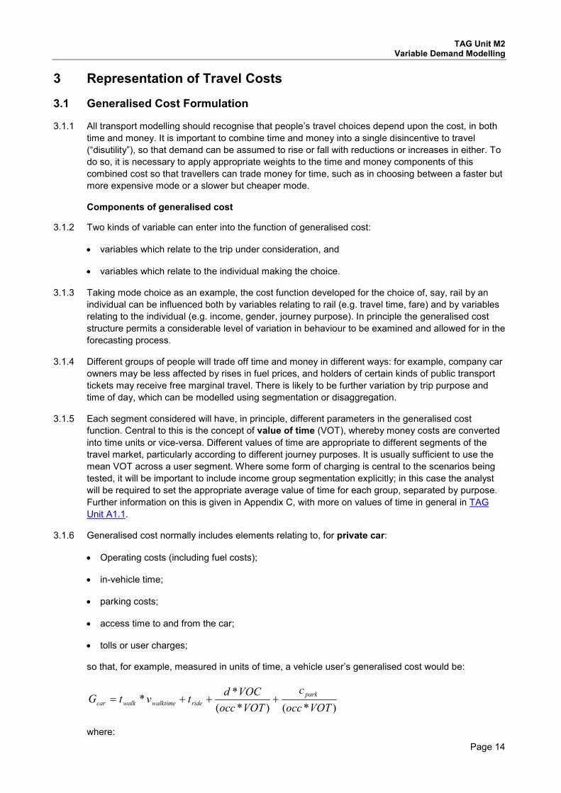
3.1.6 Generalised cost normally includes elements relating to, for private car:
• Operating costs (including fuel costs);
• in-vehicle time;
• parking costs;
• access time to and from the car;
• tolls or user charges;
so that, for example, measured in units of time, a vehicle user’s generalised cost would be:
)*()*(**
VOToccc
VOToccVOCdtvtG park
ridewalktimewalkcar +++=
where:

TAG Unit M2 Variable Demand Modelling
Page 15
twalk is the total walk time to and from the car;
vwalktime is the weight to be applied to walking time (see below).
tride is the journey time spent in the car;
VOC is the vehicle operating cost per km for a journey of d km, dependent on purpose3;
occ is the number of people in the car (who are assumed to share the cost);
VOT is the appropriate value of time; and
cpark is the parking cost.
3.1.7 Although in this formulation the generalised cost is measured in time, it can just as easily be expressed in monetary units by multiplying the whole equation by VOT4. Similarly, out-of-pocket monetary costs such as parking charges and tolls may needed to be added. These would be converted into generalised cost units by dividing by the relevant value of time.
3.1.8 For public transport modes generalised cost will include:
• fares,
• in-vehicle time,
• walking time to and from the service,
• waiting times,
• interchange penalty,
• non-walked access, e.g. park and ride,
so that, for example, in time units
erchangefare
ridewaittimewaitwalktimewalkPT cVOTc
tvtvtG int** ++++=
where:
twalk is the total walking time to and from the service;
twait is the total waiting time for all services used on the journey;
vwalktime and vwaittime are the weights to be applied to time spent walking and waiting;
tride is the total in-vehicle time;
cfare is the fare;
VOT is the appropriate value of time for the user segment; and
cinterchange is the interchange penalty if the journey involves transferring from one service to another (I is normally calculated as a time penalty multiplied by the number of interchanges).
3 Note the advice in TAG Unit A1.4 is to assume that travellers in course of work (Employer’s Business) take into account fuel cost and other operating costs of travel, whilst private travel only takes into account the cost of fuel. 4 To derive the vehicle cost in monetary units, multiply by (occ*VOT).

TAG Unit M2 Variable Demand Modelling
Page 16
3.1.9 Values of walk and wait times and interchange penalties are usually related to the value of in-vehicle time by applying weights such as vwk or vwt above. For instance, waiting time is often valued at around double the in-vehicle time. Further guidance on these weightings can be found in the generalised cost section of TAG Unit M3.2 – Public Transport Assignment Modelling.
3.1.10 It should be noted that there are other factors that affect travel choices. Probably the most important omission is that of reliability. These effects are potentially important, although mechanisms whereby reliability can be included in the generalised cost formulation are currently under development. An interim approach to estimating reliability benefits is given in the Reliability Impacts section in TAG Unit A1.3 – User and Provider Impacts as a post-model calculation. It should be noted that reliability is not included in the illustrative parameter values in Section 5.6.
3.1.11 For public transport schemes, the effects of comfort may need to be represented. Stated Preference (SP) exercises have produced plausible results whereby time spent in crowded or standing conditions incurs a higher cost than time spent seated in relative comfort (see TAG Unit M3.2). In these circumstances the estimation of the generalised costs of using public transport has an additional cost related to the degree of overcrowding, which in turn depends upon the number of passengers and capacity of the service, in terms of seating and standing capacity. To be effective, models including an overcrowding feature need to be embedded in a feedback procedure so that they are demand-sensitive. In principle this is necessary if overcrowding changes significantly in either the base or forecast situations.
3.1.12 The example below, from a rail model, shows how the impact of seating and standing capacity can be modelled as influencing the perceived journey time by using a Crowding Factor Fc:
1 when sCV *6.0≤
=cF ss CCV *4.0/)*6.0(*12.01 −+ when ss CVC ≤≤*6.0
)]*35.025.1(*)(*12.0[*1 )()(1
sCtCsCV
ssV CVC −−+−++ when CsV ≥
where
V = volume;
Cs = seating capacity; and
Ct = total capacity seating and standing.
In this model, the Crowding Factor increases the cost of in-vehicle time by a factor which is zero when 60% of the seats are occupied, rising to 1.12 when all the seats are occupied and to 2 when all the standing room is full.
3.1.13 In general, because the generalised cost methodology is relatively robust, the inclusion of additional elements does not present major modelling problems for demand forecasting. If required, it should be possible to build models that extend the standard definition of generalised cost, and also allow for greater behavioural variation between person-types and purposes.
3.1.14 All the above discussion has related to a (dis)utility function where the generalised cost is made up of a weighted linear combination of quantities such as time, distance toll etc. It is however possible that the (dis)utility function may include these quantities in a non-linear form e.g. costs may be expressed logarithmically. In these situations the concept of generalised cost, measured in time units with a constant relationship between time and cost quantities, does not hold.
3.2 Composite Costs
3.2.1 Unless mechanisms at two adjacent levels in the hierarchy are calculated simultaneously (which may be the case where levels have the same sensitivity), it is necessary to formulate a composite
TAG Unit M2 Variable Demand Modelling
Page 17
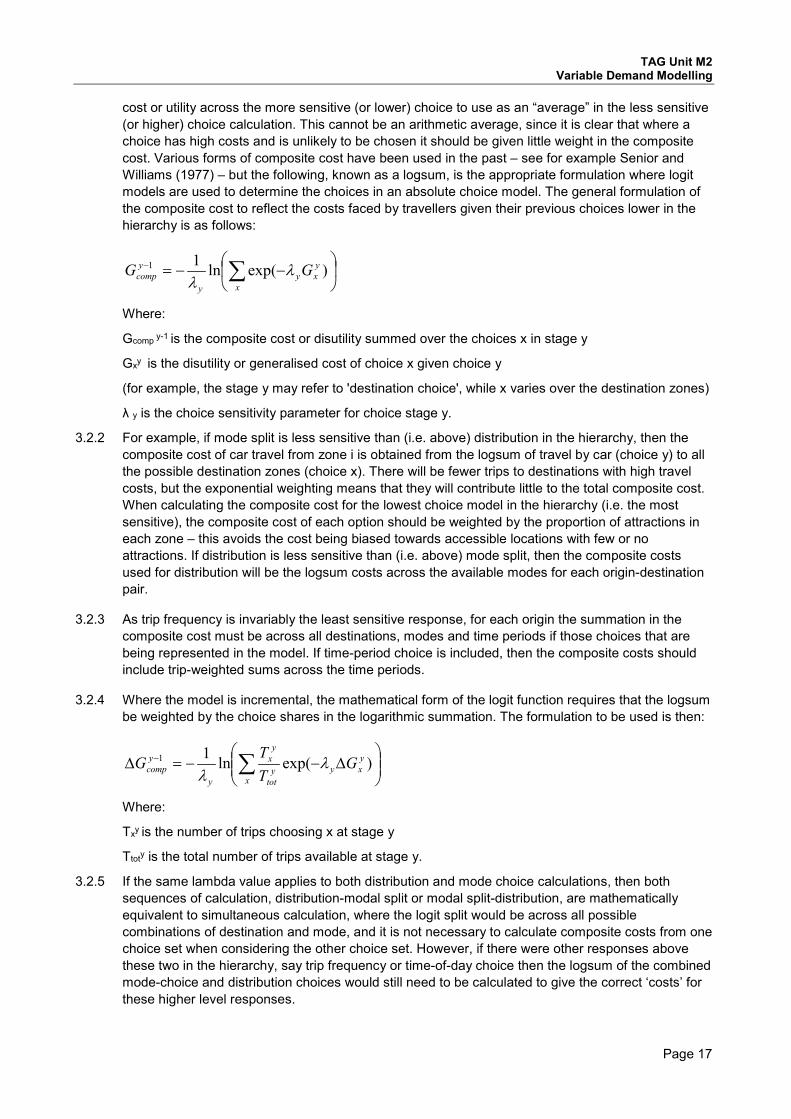
cost or utility across the more sensitive (or lower) choice to use as an “average” in the less sensitive (or higher) choice calculation. This cannot be an arithmetic average, since it is clear that where a choice has high costs and is unlikely to be chosen it should be given little weight in the composite cost. Various forms of composite cost have been used in the past – see for example Senior and Williams (1977) – but the following, known as a logsum, is the appropriate formulation where logit models are used to determine the choices in an absolute choice model. The general formulation of the composite cost to reflect the costs faced by travellers given their previous choices lower in the hierarchy is as follows:
−−= ∑−
x
yxy
y
ycomp GG )exp(ln11 λ
λ
Where:
Gcomp y-1 is the composite cost or disutility summed over the choices x in stage y
Gxy is the disutility or generalised cost of choice x given choice y
(for example, the stage y may refer to 'destination choice', while x varies over the destination zones)
λ y is the choice sensitivity parameter for choice stage y.
3.2.2 For example, if mode split is less sensitive than (i.e. above) distribution in the hierarchy, then the composite cost of car travel from zone i is obtained from the logsum of travel by car (choice y) to all the possible destination zones (choice x). There will be fewer trips to destinations with high travel costs, but the exponential weighting means that they will contribute little to the total composite cost. When calculating the composite cost for the lowest choice model in the hierarchy (i.e. the most sensitive), the composite cost of each option should be weighted by the proportion of attractions in each zone – this avoids the cost being biased towards accessible locations with few or no attractions. If distribution is less sensitive than (i.e. above) mode split, then the composite costs used for distribution will be the logsum costs across the available modes for each origin-destination pair.
3.2.3 As trip frequency is invariably the least sensitive response, for each origin the summation in the composite cost must be across all destinations, modes and time periods if those choices that are being represented in the model. If time-period choice is included, then the composite costs should include trip-weighted sums across the time periods.
3.2.4 Where the model is incremental, the mathematical form of the logit function requires that the logsum be weighted by the choice shares in the logarithmic summation. The formulation to be used is then:
∆−−=∆ ∑−
x
yxyy
tot
yx
y
ycomp G
TT
G )exp(ln11 λλ
Where:
Txy is the number of trips choosing x at stage y
Ttoty is the total number of trips available at stage y.
3.2.5 If the same lambda value applies to both distribution and mode choice calculations, then both sequences of calculation, distribution-modal split or modal split-distribution, are mathematically equivalent to simultaneous calculation, where the logit split would be across all possible combinations of destination and mode, and it is not necessary to calculate composite costs from one choice set when considering the other choice set. However, if there were other responses above these two in the hierarchy, say trip frequency or time-of-day choice then the logsum of the combined mode-choice and distribution choices would still need to be calculated to give the correct ‘costs’ for these higher level responses.

TAG Unit M2 Variable Demand Modelling
Page 18
3.3 Cost Damping
3.3.1 There is strong empirical evidence that the sensitivity of demand responses to changes in generalised cost reduces with increasing trip length (see, for example, Daly (2008, 2010)). In order to ensure that a model meets the requirements of the realism tests specified in Section 6, it may be necessary to include this variation. The mechanisms by which this may be achieved are generally referred to as ‘cost damping’.
3.3.2 Cost damping functions of one of the forms specified below should generally be used. Should analysts wish to use other forms of cost damping than those listed below, they should consult the Department before doing so.
3.3.3 Cost damping is part of our current best understanding of travel behaviour and would be expected to be incorporated into models. There are, however, some contexts where the range of travel distances that need to be represented in a transport model are limited. This might, for example, apply to some smaller interventions. In circumstances where this is not immediately clear, it would be prudent to review the range of travel distances that need to be modelled and justify the use of simpler functional forms (i.e. where values of time do not vary with distance).
3.3.4 It is not necessary for analysts to conduct tests using each of the forms specified below and to prove that one is better than the others. This is because the form of cost damping and the cost damping parameter values will interact with other aspects of the model, such as the demand model parameter values and values of time. While the cost damping parameter values, demand model parameter values and values of time should all be kept within certain limits specified below and in Section 6, it is the performance of the combination of all these aspects of the model in yielding satisfactory realism test results that is important.
3.3.5 If cost damping is employed, it should apply to all person demand responses. The same cost damping function should be applied to both car (private) and public transport costs. While the starting position should be that the same cost damping parameter values are used for both modes, it may be necessary to vary the cost damping parameters between the modes in order to achieve satisfactory realism test results. It may also be necessary to vary cost damping parameters by trip purpose. However, these variations by mode and purpose should be avoided unless it is essential to achieve acceptable model performance.
Varying Value of Time with Distance
3.3.6 Research undertaken for the Department has demonstrated that for all trip purposes there is a relationship between travel distance and the value of travel time savings (DfT, 20155). This evidence indicates that travellers’ sensitivity to cost declines more rapidly with distance than their sensitivity to time. The implication is that it is likely to be beneficial to express this in the utility function.
3.3.7 The implementation of this form of cost damping, given the emergence of this evidence, is likely to be valuable in improving model estimation and calibration and hence it is recommended to investigate this functional form during this process.
3.3.8 Varying the value of time with distance may be achieved using the following formulation:
dVOTctG +=′′′
where;
ct, are the trip time and money cost, respectively (see footnote to paragraph 3.3.11);
dVOT is the value of time which varies with distance and is specified as follows:
5 'Provision of market research for value of travel time savings and reliability: Phase 2 Report' (DfT, 2015)

TAG Unit M2 Variable Demand Modelling
Page 19
dVOTcn
ddVOT
=
0
.
where:
d is the trip length;
0d is the distance (in kilometres) underpinning the national average values of time;
VOT is the average value of time;6 and
cn is the distance elasticity which must be non-negative and less than unity, (0.248 for commuting, 0.315 for other,7 0.387 for car EB and 0.435 for rail EB); and
G ′′′ is the modified generalised cost.
3.3.9 d should be calculated by skimming distances along minimum distance paths built between all origin-destination pairs using a base year network. In forecasting, there would only be a need to recalculate these distances if the structure of the network changed significantly between base and forecast years8.
3.3.10 Models which have varied the value of time with distance have found it necessary to apply a minimum distance cut-off, cd , as follows:
dVOTcn
c
dddVOT
=
0
),max(.
where;
cd is a calibrated parameter value designed to prevent short-distance trips, particularly intra-zonal trips, becoming unduly sensitive to cost changes.
Note that, if a cut-off is used, it needs to be applied before calibrating 0d to correct the average value of time.
Damping Generalised Cost by a Function of Distance
3.3.11 Damping generalised cost by a function of distance may be achieved using the following formulation:
).()/( VOTctkdG +=′ −α ,
where;
ct, are the trip time and monetary cost9, respectively;
VOT is the value of time;
6 Appropriate assumptions for d0 and the average VOT can be found in annex C of this guidance unit. 7 These elasticities have been taken from the DfT (2015) research. 8 The reason for this is that there may be significant changes in distance travelled between the same zone pairs in a future network, for example a new estuary crossing. Using the most appropriate distance should yield more suitable damping of costs and accuracy in the demand model. This is a separate issue from distance used in appraisal, which is discussed in TAG Unit A1.3 – User and Provider Impacts. 9 Money costs include private car fuel, parking, tolls and charges and public transport fares.

TAG Unit M2 Variable Demand Modelling
Page 20
)( VOTct + is generalised cost;
G′ is the damped generalised cost;
d is the trip length10; and
α and k are parameters that need to be provided or calibrated.
3.3.12 α must be positive and less than 1 and should be determined by experimentation in the course of adjusting a model so that it meets the requirements of realism tests, as advised in Section 6. Also, if used in conjunction with variation in the value of time with distance, a further restriction on the value of α would apply (as explained below).
3.3.13 k must also be positive and in the same units as d. The ways in which its value may be determined include:
• set to the mean trip length for the modelled area; or
• set to the national mean trip length; or
• experiment to find an appropriate distance such that the results of the realism tests and any necessary model adjustments accord with the advice in Section 6.
3.3.14 Models that have used this form of cost damping have found it necessary to apply a minimum distance cut-off, below which the cost damping does not apply. The purpose of such a cut-off is to prevent short-distance trips, particularly intra-zonal trips, becoming unduly sensitive to cost changes. If a cut-off is used, it would be necessary to specify the distance below which generalised costs would not be reduced, that is the distance, d ′ , up to which )( VOTct + would apply. When a
cut-off d ′ is applied, k effectively needs to be set equal to d ′ , so that G′ is a continuous function of d at the cut-off (i.e. if a cut-off is used, the analyst should ensure that there are no discontinuities in the function).
3.3.15 Commonly used parameter values are as follows:
α = 0.5;
k = 30 km; and
d ′ = 30 km.
These values are provided merely to give an idea of the values that might be appropriate.
Power Function of Utility
3.3.16 Cost damping may also be affected by use of the following power function of utility:
βµGG =′′ ,
where;
ct, are the trip time and monetary9 cost, respectively;
VOT is the value of time;
10 This should be calculated in the same way as discussed in paragraph 3.3.9.

TAG Unit M2 Variable Demand Modelling
Page 21
G is generalised cost;
G ′′ is the damped generalised cost; and
βµ, are coefficients, which must be positive.
3.3.17 β must be greater than zero but must not exceed unity. Both β and µ should be determined by experimentation in the course of adjusting a model so that it meets the requirements of realism tests, as advised in Section 6.
3.3.18 In some applications, β has been set at values ranging from 0.65 to 0.9 and then µ has been
defined so as to set )( VOTctg += at a specified generalised cost, such as the mean generalised cost.
Combinations of Mechanisms
3.3.19 In some models, varying values of time with distance has been used in combination with damping
generalised cost by a function of distance. If this combination is used, then α + cn must be less
than 1 (which is feasible if values α and cn of the order of magnitude indicated above are used).
3.3.20 Varying values of time with distance may also be used in combination with the power function of
utility form of cost damping. If this combination is used, then both β and cn must satisfy the same limits as if the mechanisms had been used separately (i.e. both of them need to be between zero and unity).
Log Cost plus Linear Cost
3.3.21 Some models have used a log cost term in the utility function instead of the linear approach advised in the previous section. Recent research for the Department has shown that, in some cases, a better fit to the data may be obtained by a combination of log cost and linear cost, as follows:
cctG γδε +++= )log(ˆ
where;
G is generalised cost defined as a combination of log cost and linear cost;
ct, are the trip time and monetary cost, respectively;
δ is a small constant (e.g. 1 pence); and
γε , are coefficients which must be positive and would be better determined by statistical estimation rather than by experimentation.
3.3.22 When models of this type are used, the implied value of time can be obtained from the formula:
( )cVOT
εγ +=
1
These values of time need to be reported and acceptable over all appropriate values of c .

TAG Unit M2 Variable Demand Modelling
Page 22
Application of Cost Damping in Composite Cost Calculations
3.3.23 If cost damping is employed, the generalised costs used at the bottom of the choice hierarchy should be those obtained by the application of cost damping. At each higher level in the choice hierarchy, the composite costs should be calculated in the standard manner.

TAG Unit M2 Variable Demand Modelling
Page 23
4 Model Form and Choice Responses
4.1 Background
4.1.1 This Section provides the detailed advice required for those carrying out variable demand modelling after preliminary procedures have been undertaken and the scope of the model has been considered (Section 2).
4.1.2 The key summary of this part of the advice is as follows:-
• Most variable demand models use some form of “hierarchical logit” formulation (introduced in Section 4.2), in which the choice between travel alternatives depends upon an exponential function of the generalised cost or disutility (discussed in Section 4.5).
• It is recommended that demand models are applied incrementally in most cases, although absolute modelling methods may be used, applied directly or in an incremental manner (Section 4.3).
• It is expected that distribution models will be included in all variable demand models. Details of the different model formulations are discussed, as is the representation of the fringes of a study area, which is particularly important when using trip distribution models (Section 4.6).
• The representation of different modes in the variable demand model is discussed, including how it may be necessary to model journey components in detail, including the effect of changing road conditions on bus travel, or whether it is acceptable to include alternative modes as a set of fixed costs (Section 4.7).
• The modelling of departure time choice as a demand response or in close association with assignment is discussed. It is recommended that large "macro" adjustments only need to be modelled when considering differential pricing between time periods, or access restrictions (Section 4.8).
• Where highway costs are important, a variable demand model will need to include a highway assignment stage to provide cost information to the demand model (Section 4.10).
4.2 Functional Form
4.2.1 Any model of the demand for travel relies on a mathematical mechanism that reflects how demand will change in response to a change in generalised cost. These are discussed in detail in Appendix D.
4.2.2 Most variable demand models use some form of “hierarchical logit” formulation, in which the choice between travel alternatives (frequency, modes, destinations, time periods) depends upon an exponential function of the generalised cost or disutility.
4.2.3 A single logit model may be applied to the entire range of choices available using a multinomial logit model. However, that would implicitly assume that the sensitivities of those choices were all the same. This is unlikely to be the case. This leads to a hierarchical system of logit formulations in which at each level a limited number of choices are considered. For example, a variable demand model might:
• first estimate the number of trips from any given origin (trip frequency - usually as an elasticity formulation);
• then estimate how many trips will choose each available mode (mode split); and
• then estimate how these trips choose amongst the available destinations (trip distribution).

TAG Unit M2 Variable Demand Modelling
Page 24
(Note: this example excludes any time of day choice mechanism.)
4.2.4 The sequence appropriate often varies between types of trip and does not necessarily represent the sequence of thought that makes these decisions. All the choices are interconnected, so that in a model that is converged, choices made earlier in the sequence are consistent with choices later in the sequence as the calculation is repeated.
4.2.5 Choices made higher in the hierarchy act as constraints on those made later. Hence, if the sensitivity of choice decreases down the sequence there is a danger of later choices being too strongly influenced by earlier choices. Further discussion of the hierarchy of responses can be found in Section 4.5.
4.2.6 Within any of the steps (known as hierarchical levels), it may be desirable to model some secondary choices, for example, because travellers seem not to discriminate between different public transport modes in the same way as they treat the choice between car and public transport. Consequently, it may be preferable to split mode choice into a “high-level” two-way choice between car and public transport, with a “lower level” split into the different public transport modes. This is often referred to as nested logit. It avoids the common problem with forecasting trips across three modes, car, bus and rail, of making the choice over-sensitive to changes in what travellers perceive as competing public transport services.
4.3 Form of Models
4.3.1 An important issue that needs to be decided is the form of the demand model used for particular applications. There are a number of model forms that can be employed and these can generally be placed into three categories:
• absolute models, that use a direct estimate of the number of trips in each category;
• absolute models applied incrementally, that use absolute model estimates to apply changes to a base matrix; and
• pivot-point models, that use cost changes to estimate the changes in the number of trips from a base matrix.
The choice of which form of model would depend on the compatibility of the base demand matrix if in P/A format (see Section 2.5) and the assignment matrix used.
4.3.2 The latter two methods in the above list retain all the detail of the observations, but generally face difficulties where too many (or key) cells in the observed matrices are empty because of the limited amount of surveying possible. This section explains the differences and the preferred approaches.
Absolute Models
4.3.3 Absolute demand models generate estimates of trip numbers, based on a model that is calibrated to fit as closely as possible to the known observed movements and the resulting model is used to directly forecast future trips. Base year and forecast trip patterns are produced independently of each other, using common model parameters. The sensitivity parameters used in absolute models should be calibrated from local data. In addition to the calibrated sensitivity parameters, however, mode-specific and movement-specific constants will usually be required to achieve an acceptable fit to the observed data.
4.3.4 The fit of these models to the observed base year data can often be quite poor, or particularly challenging and time consuming to calibrate satisfactorily, even where calibration constants disaggregated by area type are used.

TAG Unit M2 Variable Demand Modelling
Page 25
Absolute Models Applied Incrementally
4.3.5 In more recent practice, forecasting approaches have attempted to make use not only of the absolute model but also the ‘observed’ base trip matrices on which it was calibrated. This could be by factoring the forecast trip matrices by the ratio of the base year synthesised matrix to that of the base year observed matrix, so that:
Future year matrix = (Base year observed matrix / Model absolute base year matrix) * Model absolute future forecast
4.3.6 However, this could lead to odd results where the cells of the observed trip matrix are zero. A way around this problem that has been used by some multi-stage models is to employ an additive approach so that:
Future year matrix = (Model absolute future forecast - Model absolute base year matrix) + Base year observed matrix
4.3.7 Thus, the future forecast by the model is increased by the difference between the base year observed trip matrices and those produced in the base year by the model. The danger with this approach is that negative cell values could result.
4.3.8 In either of these two approaches the important differences between the observed matrices and the base year model that were not picked up in the calibration process are reflected in the forecasts.
Pivot-Point Models
4.3.9 Pivot-point models estimate changes in trip patterns relative to a base matrix in which, normally, observed movements are used as much as possible. Such model applications are often described as ‘incremental’ or ‘marginal’. The predicted relative changes are applied to the base matrix, so that the complexities of the base matrix are preserved. Where it would be difficult to calibrate a demand model to reproduce the observed pattern of travel these incremental models can be used to predict from (pivot off) this base matrix and associated costs. The matrix can also be updated in whole or in part without altering the forecasting model since the parameters controlling the mechanisms can be independent of the calibration of the base model.
4.3.10 With true incremental models the base year conditions (costs) and the reference trip pattern (derived from the base year trip matrix assuming no changes in travel costs) are direct inputs to the forecasting process. Such an approach can use existing data relatively easily, and the parameters used in the model can reflect known sensitivities to changes in input variables without having to perform the additional and time-consuming task of fitting to an observed pattern. The parameters will generally need to be calibrated using external data sources, or imported from other demand models (see Appendix G, which discusses transferring mode choice model systems and Section 5.5, which discusses illustrative parameter values). Models that use this approach to forecasting are described further in Section 6.
4.3.11 The principles of the recommended pivot-point approach to forecasting, i.e. the way that the forecasts pivot off the base year costs, are explained in more detail in TAG Unit M4 – Forecasting and Uncertainty.
Choice of Model Form
4.3.12 The Department’s recommendation for scheme appraisal is to use an incremental form of model, whether pivot-point or based on incremental application of absolute estimates, unless there are strong reasons for not doing so. Such reasons could include situations where there are large changes in land use between the base and forecast years, which will significantly change the distributions of origins and destinations.
4.3.13 ’Observed’ trip matrices drawn from survey data that are used in incremental models are likely to contain a very high proportion of cells with zero trips. Without importing synthetic data an

TAG Unit M2 Variable Demand Modelling
Page 26
incremental model will never fill these cells. If the travel that the cell represents is truly infeasible then zero trips may be a reasonable assumption, but if the cell is empty merely because of sample limitations some matrix infilling will be essential. These infilling techniques are discussed in detail in DMRB Volume 12.1.1.
4.3.14 In contrast, absolute forecasting models use observed data for calibration purposes. In practice, often a large number of calibration factors need to be used with most absolute models to provide a reasonable fit to these data, often in a rather arbitrary way, especially in the case of distribution models. In addition the parameter values so obtained may have arisen from some masking of observed differences (which may for example be distance-related effects) by the zonal or mode specific constants and may therefore either underestimate or exaggerate the true sensitivity of travellers to changes. Consequently, the apparent superiority of local calibration is often not fulfilled in practice except in large-scale transport studies, where the data collection and calibration can be sufficiently comprehensive.
4.3.15 Pivot-point approaches are attractive, but it is necessary to sound a note of caution. Any deliberate decision not to attempt to synthesise observed cross-sectional variation has potential forecasting implications. To the extent that a model is deficient in synthesising, it may be equally deficient when used incrementally. This is called model misspecification.
4.3.16 However, the observed data are themselves affected by sampling error considerations. One way around this problem is to use a mixture of observed and synthesised data, even for movements supposedly wholly observed, particularly where sample sizes are small and sampling error consequently high. The relative quality of the data and the synthetic model need to be considered, especially if long-term redistribution processes might not have been fully realised.
4.3.17 However, by taking a weighted average of the observed and synthetic matrices empty cells are eliminated and greater weight is given to cells where there are more observed trips than expected from the locally-calibrated synthetic model. Relative weights should reflect the relative accuracy of the two forms of estimates. Synthesised data is also required for movements not captured by the survey strategy.
4.3.18 The main problem with using pivot-point models occurs when the base matrix contains few or no trips for a set of movements, but the forecasts expect large changes in these movements to occur. This often arises when a zone is re-developed or has no trips to or from it in the base situation. In these situations the forecast will have to be synthesised exogenously for these movements.
4.4 Model Interfaces
4.4.1 It is essential that the demand and assignment models are correctly connected, with consistent cost definitions and appropriate conversions between the P/A demand model matrices and the assignment O/D matrices.
Matrix Conversion
4.4.2 The conversion from P/A to O/D matrices (all or most of the day to specific time periods) is usually done after time of day choice, distribution and mode choice and before assignment. P/A based trips are converted into O/D based trips by using conversion factors disaggregated by time of day and trip purpose (distinguishing between from and to home ,home-based trips). Although these factors may change over time in reality, it is usually acceptable practice to assume constancy before any time-period choice is applied. Such factors can be obtained locally or by using NTS data tables (this is how NTEM produces O/D based forecasts from P/A forecasts). Indeed, this conversion is available in the TEMPRO software and may be used as a default way to achieve this conversion.
4.4.3 Demand changes to the base P/A matrix may then be modelled either absolutely or incrementally. Where modelling incrementally, the base values are incorporated explicitly in the demand formulation. In the case where the adjustments to the P/A matrix do not provide a “compatible” O/D

TAG Unit M2 Variable Demand Modelling
Page 27
matrix, only the implied change in demand after converting to O/D form is used to adjust the base assignment matrices.
4.4.4 Whilst highway assignment modelling is concerned with vehicle movement, demand modelling is concerned with individual traveller decisions. Before the highway assignment stage is reached, car occupancy factors need to be applied to the private travel demand matrices to convert them to vehicles. Data Book Table A1.3.3 gives default values by trip purpose and time period, as well as assumptions about how these factors are expected to change through time. Local factors can be calculated from RSI data to see if there are other local factors affecting car occupancy, such as direction of travel or type of flow. These local factors should be used if there are significant differences from the national ones and if there is confidence that the RSI-based factors are an unbiased estimate of all vehicle travel in the area.
Feeding Back Costs from Assignment to Demand Model
4.4.5 The assignment model provides the travel times and costs required by the demand model, and generally both assignment and demand models will use costs averaged across the defined time periods into which the model has been divided. In principle, models should calculate trip-weighted cost averages across the time periods according to the number of trips in each period (which is the approach adopted in DIADEM, see Appendix H). Note that in the demand model these average costs for particular types of trips may be averaged again across different modes, or different destinations, to obtain the “composite” costs on which the demand mechanisms operate.
4.4.6 The trip-weighted average approach requires an adequate level of detail in the model. Where this is not the case, some models relate all demand in a given purpose category to the costs in the period where most of these trips are made. Depending on which trip purposes are categorised in the model, the cost bases may be approximated as follows:
Table 4.1 Approximate Cost Bases for Each Trip Purpose Trip purpose Cost base home-based journey to/from work peak period costs home-based education peak period costs home-based shopping off-peak11 or interpeak period costs home-based leisure/recreation off-peak or interpeak period costs home-based social/personal business off-peak or interpeak period costs home-based employer’s business peak period costs home-based other off-peak or interpeak period costs non-home-based employer’s business off-peak or interpeak period costs non-home-based other off-peak or interpeak period costs
4.4.7 Few models have as detailed a disaggregation of trip purposes as listed in Table 4.1 and it is usual
to aggregate them into fewer categories (home-based shopping, leisure and social are often combined into “other” category, for example). For each category, the mean generalised costs of travel in the appropriate period, or in a combination of periods (or sub-periods) weighted according to the proportions of trips in each, are calculated and fed back to the demand model. Where the assignment model used is dynamic, or quasi-dynamic, mean costs can be obtained on a flow-weighted basis taking proper account of the variation over time, but the mean across the broader time periods should still form the basis of the demand modelling.
11 It should be noted that off peak costs (the period outside of the AM peak, inter-peak and PM peaks) can have sufficiently different costs from the inter-peak period. The analyst should of course choose the most representative costs for each purpose in order to minimise bias in the demand model.

TAG Unit M2 Variable Demand Modelling
Page 28
4.5 Hierarchy of Choice Responses
4.5.1 As described in previous Sections, the main choice response mechanisms that are considered in variable demand models are as follows:
• Trip Frequency;
• Mode Choice;
• Time of Day Choice (Macro and/or Micro Time Period Choice);
• Destination Choice (Trip Distribution);
• Route Choice (Assignment).
These choice responses are described in more detail in Sections 4.6 to 4.10. These choices are not exclusive and others may be included, such as micro time period choice or other subsidiary choices, e.g. parking models.
4.5.2 Once decisions have been made on which responses to include in the model, the hierarchy in which those responses are considered must follow certain rules. This is not simply a question of mathematical or computational convenience. The sequence of the mechanisms is important to the overall outcome, and the resultant elasticities of demand and the predicted travel pattern will be affected by it. This section describes how the hierarchy should be determined.
4.5.3 The appropriate hierarchy or sequence of choice mechanisms must be determined by the relative sensitivities (the lambdas of a logit model) of the choices to the generalised costs or disutilities of travel. Different sequences for different purposes and/or segments of the travel market are often appropriate.
4.5.4 A mechanism placed higher in the hierarchy of demand mechanisms should reflect the composite cost of choices lower in the hierarchy and allow for how a choice with high costs is unlikely to be chosen. A logsum of costs has that property, but requires higher demand mechanisms to have a smaller sensitivity, to avoid a plausible change in generalised cost producing an implausible shift in demand.
4.5.5 The sequence of calculations is that, during each cycle, the composite costs must be calculated for each level in the hierarchy, since each level refers to different combinations of choice lower in the hierarchy (see Section 3.2 for further detail on composite cost calculations).
Figure 4.1 A Typical Choice Hierarchy with Associated Cost Transfers
4.5.6 Thus the composite cost calculation starts at the bottom of the hierarchy and works its way up the levels, adding one more choice into the composite cost at each level. The choice calculations are
Composite cost (p,j,t,m)
Composite cost (p,j,t)
Composite cost (p)
Assignment costs
Trip Frequency
Mode choice (m)
Trip distribution (j)
Micro time period choice (p)
Assignment
Composite cost (p,j) Macro time period choice(t)
Composite cost (p,j,t,m)
Composite cost (p,j,t)
Composite cost (p)
Assignment costs
Trip Frequency
Mode choice (m)
Trip distribution (j)
Micro time period choice (p)
Assignment
Composite cost (p,j) Macro time period choice(t)

TAG Unit M2 Variable Demand Modelling
Page 29
then made down the hierarchy and the whole cycle is recalculated in the next iteration until an acceptable degree of convergence is achieved (see section 6.3).
4.5.7 Depending on their relative sensitivities, the mechanisms may need to be positioned at different places in the hierarchy. Available evidence suggests that the sensitivity of trip frequency is very much smaller than for the other mechanisms, and it is justifiable to always treat this choice as first in the hierarchy.
4.5.8 Route choice is invariably modelled as the most sensitive response below the other demand mechanisms. In equilibrium, there is little or no difference in utility or generalised cost between the routes which are likely to be used for any given origin-to-destination journey; if costs change, a new equilibrium involving some change of route between the minimum cost alternatives is quickly established. Thus the route assignment part of the modelling can be considered separately, though of course demand and assignment must be executed iteratively to obtain an equilibrium solution.
4.5.9 Where macro time period choice is thought applicable (where there are expected to be differential changes in the costs or capacity in different time-periods) evidence suggests that the position of this mechanism is at a similar level to main mode choice for most purposes.
4.5.10 Where micro time period choice is being modelled, this should be placed above assignment but otherwise at the lowest level (most sensitive) of the hierarchy.
4.5.11 The main decision centres on the relative positions of distribution (destination choice) and mode split (choice).
4.5.12 Where sufficient local data of suitable quality exist, and the skilled resources required are available, lambda values should be estimated (calibrated) from that data and the hierarchy selected so that the less sensitive of the two responses is positioned above the more sensitive.
4.5.13 Where this is not the case, then it may be possible to select the hierarchy on the basis of local evidence about the relative sensitivities of destination and modal choice from existing local models where the lambda values have been estimated and the adopted choice hierarchy has been justified. If estimated parameters for mode and destination choice are very similar, there may be a case for simultaneous calculation using a single lambda value for each traveller segment.
4.5.14 If there is insufficient local data or resources for estimation, and no suitable local model from which the parameters can be transferred, it will be necessary to consider the illustrative values provided from Section 5.6 as the basis for the choice hierarchy. All the models used to derive the illustrative parameter values were rigorously calibrated against local data and all showed that main mode choice was less sensitive than destination choice. In the absence of any information to the contrary, this is therefore the hierarchy which should be adopted.
4.5.15 However, if for example, destination choice has a larger sensitivity parameter than mode choice, yet mode split was mistakenly calculated after distribution, an increase in the cost of, say, car travel might increase the mean (composite) cost of travel on which distribution is based. In extreme cases that could shorten all trips to such an extent that not only is car use decreased, as required, but also travel on the competing modes, which is implausible. Such an effect is often described as a perverse cross-elasticity.
4.5.16 In a multinomial logit formulation, a given level of the main choice hierarchy may split the choice into separate sub-levels. Such “nesting” is most often met in mode choice, where the split between competing public transport modes is made at a lower level than the primary split between car and public transport (and possibly the active modes also). This avoids the “red bus/blue bus problem” where separating the bus mode into two without nesting apparently affects the predicted total bus share. Nested logit can be applied to other demand mechanisms; however, as for example in a time-period split between broad peak and off-peak periods, and then subsequently between

TAG Unit M2 Variable Demand Modelling
Page 30
narrower periods within the peak. Nesting can also use high-level large zones in distribution, and subsequently a further distribution within the larger zone to finer zones, but this is likely to be relevant only to more specialised models than the ones addressed by this advice.
4.5.17 Whichever approach is adopted, it is essential to apply “realism testing” to a broad range of transport changes (see Section 6) to ensure that the model responds rationally and with acceptable elasticities.
4.6 Trip Frequency
4.6.1 Trip frequency models represent the response of trips to changes in generalised costs. This is distinct from trip generation, which estimates trips based on the demographic and socio-economic characteristics of an area. If the population or car ownership or built development of the area is changing appreciably over the time period of interest, an explicit trip generation mechanism should be considered, i.e. a trip end model. Where this is not a requirement, NTEM provides growth forecasts of trip productions and attractions.
4.6.2 The inclusion of a trip frequency response requires the incorporation of the elasticity mechanism to represent trip frequency as described in Appendix D.
4.6.3 Where the active modes of walk and cycle are not explicitly included in the demand model, trip frequency may be thought of as, mainly, the transfer between the active modes and the mechanised modes. Otherwise, overall trip rates will be fairly stable and there will often be no need to model the response of trip frequency to changes in travel cost since the effect of trip frequency is likely to be small. It may therefore be proportional to omit this response, particularly since the frequency effect is markedly less important than the other choices and there is little evidence to justify the scale of frequency parameters and elasticities by purpose.
4.6.4 The trip frequency sub-model, when used, should apply at the total motorised mode level, and separately by trip purpose. A single frequency lambda parameter should initially be adopted for each purpose without distinction by car ownership or availability. As with other choice parameters, adjustments may be required and variations by car availability introduced to ensure the demand elasticities generated by the realism tests accord with established values.
4.6.5 There will not normally be a requirement to model trip frequency for doubly-constrained trips such as commuting, since the constraints on total travel are usually assumed to be binding, since employment is assumed to be fixed. This implication does not hold if active modes have been omitted and they are likely to form a significant percentage of commuting trips, and/or the planned intervention will result in a significant impact on active mode users. These circumstances indicate that, where it has been considered that including a mode choice response for active modes is of disproportionate effort, a trip frequency response should be included if the potential impact is judged to be sufficiently large. If so, care needs to be taken that the response is not simply affecting long distance trips rather than the short distance trips the response is acting as a surrogate for.
4.6.6 It is unlikely that data will be available to enable trip frequency lambdas to be estimated locally. In general, trip frequency lambdas should be imported rather than estimated.
4.7 Mode Choice
Which Modes at What Detail?
4.7.1 Usually, the main alternative mode to car will be public transport in its various forms and vice versa. Depending on the nature of scheme and its expected impacts, it may also be desirable to represent competition from walk and cycle.
4.7.2 It is almost always desirable to include some representation of modal choice in variable demand modelling, but the level of detail depends upon the importance attached to it. It may be acceptable to include the alternative mode(s) merely as a set of fixed costs, but it may be necessary to model

TAG Unit M2 Variable Demand Modelling
Page 31
the journey components in detail, including for example the effect of changing road conditions on bus travel times.
4.7.3 A few models omit the mode choice mechanism altogether because modal transfer is not considered to be important. This is not recommended in most cases (see Section 2.3), but if that approach is used it will be important to include a trip frequency elasticity at a greater strength than usual, since this will act as proxy for trips transferred to the car mode from other modes and vice versa.
4.7.4 If there is little real competition between private and public transport and public transport is not a key focus of the intervention being tested (and the future role of public transport in the locality will not become increasingly important through other intervention), the public transport generalised cost estimates can be made with limited precision. The level of competition can best be judged from local knowledge of modal split for car-available travellers. This can be obtained by travel surveys which set out to identify car availability: in most cases it will have to be proxied by household car ownership, but this will generally overestimate true availability. Approximate values for an area can be obtained from the Census.
4.7.5 As a general guide, if public transport is chosen by less than 5% of travellers, use of fixed public transport costs will suffice, unless public transport alternatives need to be assessed as part of the scheme appraisal.
4.7.6 For rail, access to stations is likely to be by car for some trips, and a mean generalised cost of access across all relevant modes (walk, bus, and car including parking charges) should be estimated. Large changes in demand for either rail or bus might result in changes in service frequency. These effects should be examined using a specialised public transport model (see TAG Unit M3.2), from which the generalised costs for each OD can be extracted directly. Where a highway assignment model is also included, the generalised costs of the highway and public transport assignment models need to be consistent with one another.
Active Modes
4.7.7 Most scheme appraisal models will be sufficient where active modes are not included in the demand model, particularly in the case of highway schemes. However, there may be special reasons for examining the role of active modes in the modelling (for instance for schemes on radial routes in urban areas with high cycle usage) and their inclusion may well affect predictions of short trips on a road scheme.
4.7.8 When active modes are omitted trip frequency elasticities should be stronger, since then they have to represent the effect of active modal transfer. If active modes are to be included, then a cost-responsive trip frequency mechanism can be omitted altogether. If they are treated as a separate mode, as opposed to them being included in a general non-car mode, it will normally be adequate to treat their generalised costs as linearly dependent on OD distance travelled, via an average speed that is conventionally 4 km/h for walking and 12 km/h for cycling. Walking speeds in particular are a function of the number of roads crossed, and the amount of traffic on these roads, but this aspect is rarely captured in modelling.
4.7.9 Active modes may be included in mode split at either level of the hierarchy, as part of a higher level car/public transport/active mode split with perhaps a sub-modal split between walk and cycle, or, more usually, the higher level split may be kept binary between car and public transport plus active mode, and the latter split at a further nested sub-modal level.
Detail of the Model
4.7.10 In the case that more than one mode may offer a competitive alternative to car, the demand model should include a higher level private/public transport modal split mechanism, with a separate nest between the available public transport modes below this in the hierarchy (see Section 4.5). The choice sensitivity lambda parameters should be larger at these lower levels than at the higher level.

TAG Unit M2 Variable Demand Modelling
Page 32
A separate public transport assignment model is recommended where the scheme is expected to have a significant impact on public transport and/or public transport alternatives are to be tested (see TAG Unit M3.2).
4.7.11 The detail of the mode choice sub-model may not only depend on the nature of the existing public transport system and the type of scheme, but also on the nature of the passengers being served. For example, air passengers respond differently from the average traveller. People’s propensity to use public transport to and from an airport may vary markedly according to whether they are travelling on business or leisure and whether they are away from their home area. For a mode choice sub-model designed to appraise a link to an airport, therefore, the demand needs to be segmented in a different way to that used for the modelling of general travel in an urban area.
4.7.12 An initial structural issue is how mode choice and destination choice should relate to each other within the hierarchy. How the models relate to each other depends on the relative accuracy of measurement of generalised cost differences influencing the two choices. Issues such as zone size and the quality of the transport networks will therefore influence the structure. This issue is thus best left to analysis of local data.
4.7.13 It is essential that the models of mode and destination choice be properly linked through appropriate composite costs (see Section 3.2). Further, the coefficient of composite cost must have a value which lies in a specific range – depending on the exact model structure, but usually between 0 and 1 – which ensures that the responses of the model are not obviously wrong. For example, if such a constraint were not met, it might be possible that an improvement to public transport in a corridor could increase total traffic in the corridor by so much that car journeys were also predicted to increase.
Sub-mode Choice
4.7.14 Within the public transport system there may be a range of ‘sub-modes’:
• different public transport modes, i.e. bus, light rail, heavy rail;
• different access modes to public transport, i.e. walk, cycle, taxi, car (park-and-ride or ‘kiss-and-ride’).
4.7.15 Further there will be many trip options that involve combinations of public transport modes. Choices within these sub-modes can be modelled either by choice models of the form used for the main mode choice or they can be handled in the assignment procedure. This is an important decision for the design of a model and requires careful consideration.
4.7.16 A logit-based approach to choice modelling is more stable and transparent, and therefore capable of inspiring greater confidence, than an assignment-based approach. A choice model approach can also be supported by empirical evidence more easily. However, in instances where there are predicted to be significant numbers of mixed mode trips using a significant number of mode combinations, a logit-based approach can be cumbersome.
4.7.17 A logit-based approach is also preferable for situations:
• where travellers who are indistinguishable with respect to measured variables are likely to choose different alternatives in significant numbers, i.e. the split is not close to zero–one;
• where sub-mode split can only be explained by the incorporation of a constant representing the net effect of unmeasured variables in influencing the choice between sub-modes;
• where there are serious difficulties in calculating fares for trips using a mixture of sub-modes – as these can be directly incorporated in a choice model;

TAG Unit M2 Variable Demand Modelling
Page 33
• where the model includes representation of car access to public transport, because there are many household-related reasons for using or not using a car that are not clearly represented in current models. Further, assignment packages generally have difficulty with the processing needed to deal with mixed car and public transport journeys. The car access component should of course be assigned to the car network.
4.7.18 For the choice among ‘pure’ public transport alternatives (i.e. not mixed modes such as park and ride), however, the issue is not so clear and local circumstances, including software capability, will be decisive. A key issue for consideration is deriving appropriate composite cost measures for use in the main mode choice model.
4.7.19 The analyst should be aware that, even if the sub-mode choices are modelled through a choice model, the public transport assignment must produce the required skimmed time and cost values for each of the alternatives, for example by bus and train separately. Particular care must be taken that, for the sake of consistency, the assignment should reproduce the (sub)-modal splits calculated in the choice model, which may require manipulation of networks and linkages – so-called biased networks.
4.8 Time of Day Choice
4.8.1 It is unlikely that a variable demand model for a scheme will need to look at time of day choice over all 24 hours in a day but there will be circumstances where the choice of time of travel in certain parts of the day could be expected to be influenced by changing travel costs.
4.8.2 There are two distinctly different aspects of time of day choice; these are termed macro time period choice and micro time period choice. Macro time period choice represents the choice between broad modelled time periods, whereas micro time period choice represents choices within a modelled time period. Variable demand models only usually include macro time period choice if at all, to represent transfer of traffic between broad time periods, although micro time period choice has more recently been facilitated by some software packages and notably in the Department’s DIADEM software (see Appendix H).
Macro Time Period Choice
4.8.3 Macro time period choice, involving the transfer of trips between broad time periods, can be modelled as a logit choice in a similar way to the choice mechanisms described for the other stages of demand modelling. However, if the demand modelling uses the typical division of time into two peak periods and an inter-peak, the freedom of most trips to transfer between them will be severely constrained: few work trips, for example, could move outside the three-hour peak periods entirely, and such a mechanism might be applied predominantly for shopping as opposed to the journey to work.
4.8.4 To model macro choices, it is necessary to know what proportion of each type of trip takes place in each period. At a macro level trips must be allocated to a discrete time period; even those which start and finish in different periods. An incremental logit model can then be used to modify the total number of trips of each type of trip in each time period according to the changes in the mean generalised costs in each period.
4.8.5 Macro time period choice should be considered when strong cost differentials between time periods are expected to develop or change. This is obviously the case where different charges are introduced for use of a road, rail or bus service in the peak and inter peak or off-peak, or where different levels of access to road capacity are being contemplated, or perhaps where peak surcharges are introduced for parking in a way which affects a large proportion of traffic. In these cases it is obviously important to choose the modelled time periods to facilitate the modelling of the differential costs. If this mechanism is included then sensitivity testing (see Section 6) of the strength of the parameters should be used to examine the possible range of responses. it can be important to apply different sensitivity parameters to different trip purposes.

TAG Unit M2 Variable Demand Modelling
Page 34
4.8.6 Less evidence is available about the sensitivity of the macro-time period choice than either main mode or destination choice. Research conducted for the Department suggests that the sensitivity of the choice between relatively long time periods, such as three hours or so, should be about the same as that of main mode choice. The research also suggests that, as the time periods are reduced, the sensitivity increases. Thus, when long time periods, of the order of three hours, are being modelled, macro-time period choice should be positioned either just above or just below main mode choice, with parameter values similar in magnitude to the main mode choice parameter values.
Peak Spreading (Micro Time Period Choice)
4.8.7 It is common experience that when demand grows in a congested network the peak in demand tends to occupy a longer time. The peak is unable to grow higher for lack of capacity, so additional demand is accommodated in the shoulders of the peak. This effect is known as “peak spreading”, but it occurs because of a mixture of responses, both involuntary and voluntary:
4.8.8 If modelling predicts unrealistically severe congestion in the peak hour, micro time period choice modelling to reallocate trips between the peak hour and the shoulders may be used to achieve a more realistic estimate. The HADES model functionality imbedded within the DIADEM software has been developed in order to assist with this (see Appendix H). It represents a continuous range of departure times and interfaces with a range of assignment software which use a small number of time periods. For further information see https://www.gov.uk/government/publications/diadem-software.
4.8.9 The length of the peaks will spread as congestion grows, because lower speeds mean that any given journey will take longer to complete and will occupy a longer period. The traveller has little influence in this, and the delays caused by this effect are often represented within the assignment modelling itself.
4.8.10 Travellers can deliberately change their time of travel, departing and arriving earlier, or later, than their preferred time. It is common experience in congested conditions that a quarter hour change in departure time can change the expected mean travel time significantly. Some travellers will find such a change acceptable, because the saving in journey time outweighs the benefit they attach to arriving at a preferred time. The response is clearly more available for travellers who have some flexibility in precisely when they must arrive and is applicable to those work trips that have some degree of flexibility for earlier or later arrival.
4.8.11 In the face of increasing congestion, some travellers will adjust their departure times or arrival times to gain a reduction in travel time. In principle, this can be represented as a choice mechanism reflecting the generalised cost of travel to which has been added the cost of not arriving at the preferred time: this is a “schedule disutility term”, essentially an extra component to the generalised cost which measures how far the actual arrival time is before or after the preferred time.
4.8.12 When a micro time period choice response (that will include a schedule disutility term) is included in a variable demand model, evidence suggests that this is likely to be more sensitive than other responses except route choice.
4.8.13 Other techniques may be used to represent peak spreading between the peak hour and shoulders, such as multinomial logit, although there are theorectical reasons why this form of model may not be a reliable predictor of choice between shorter time periods.
4.9 Trip Distribution
4.9.1 When modelling individual variable demand responses it is expected that a distribution mechanism will be included. This can have a substantial effect on the trip pattern and the amount of traffic using the scheme.

TAG Unit M2 Variable Demand Modelling
Page 35
4.9.2 Distribution models can be applied in terms of zonal productions and attractions or less satisfactorily in terms of origin and destination trip totals.
4.9.3 It is common to use doubly-constrained models for forecasting commuting and education trips, so that each zone attracts and generates a fixed total of work trip ends, and singly-constrained models for other purposes, where only the total number of trips generated in each zone is fixed.
4.9.4 In addition to cost, distribution also depends on some measure of the attraction of a zone, estimated in terms of the numbers of “opportunities” such as jobs or retail floorspace in the zone. These reflect the likelihood that the zone will be chosen as a destination, other things being equal (though in doubly-constrained models the attraction is simply the number of trips required to end in the zone).
4.9.5 The main stumbling block in the use of distribution models lies in estimating the trip attraction factors for each zone in a robust and reliable way, and in determining parameters which have real predictive values. This is difficult, since the distribution parameters are normally calibrated to recreate the (cross-sectional) data observed at a given point in time, which depend on a wide range of historic and socio-economic factors, which cannot be captured fully in the modelled transport factors. Those historic factors can be large enough sometimes to mask the true choice process amongst closely competing destinations in an equilibrium model.
4.9.6 Consequently, the model’s ability to predict choices and changes in trip patterns due to changing transport factors is generally unproven. For this reason it is recommended that trip distribution models normally have an incremental form, building on a largely observed base. Local parameter values should be calibrated for use in the model; however, if there is insufficient observed data for satisfactory calibration, externally derived parameter values should be used, although some adjustment may be needed to deal with any under-representation of competing destinations and situations where major changes to land-use are expected to occur.
4.9.7 Predictions of trip distribution are usually “Production Constrained” to a total based on forecasts of trip-ends. Similarly, the trip matrix can be constrained to match a required number of total trip attractions. In general, the trip matrix and productions will be disaggregated by trip/traveller segments, and will have to satisfy the constraints within each individual segment, such as each trip purpose or traveller type.
4.9.8 There are four main decisions that have to be made about the use of trip distribution models within a variable demand model:
i) Production/Attraction or Origin/Destination Modelling
4.9.9 The implications for this are discussed Section 2.5 and the choice is likely to be made based on the availability of data, what other demand responses are being modelled, and what form of demand/assignment model is being used. However, when building a new model, or substantially updating one, the presumption should be that any new matrices are assembled and used as P/A defined trip matrices.
ii) Doubly or Singly Constrained
4.9.10 In general, doubly constrained models should be used for commuting and education. This reflects the relative confidence in the measures of attraction (employment and student numbers) for commuting and education trips, as well as the relatively fixed nature of these attraction values in the short term.
4.9.11 Other purposes such as shopping, social and leisure trips are typically modelled as singly production-end constrained. For these purposes, the trip end factors reflect the attraction of destinations, not the actual numbers of trips attracted and ideally the availability of intervening similar destinations between the origin zone and the zone in question. For some of these purposes it may be logical to consider a trip frequency effect on top of the distribution effect; that is decreasing

TAG Unit M2 Variable Demand Modelling
Page 36
costs will lead to greater numbers of trips of that purpose as well as change the destinations. Examples of this are leisure or holiday trips, but shopping trips are also likely to be elastic, especially if the model does not include active modes, since walk trips to the local shop may become mechanised trips to more distant shopping centres if travel costs fall.
4.9.12 In practice the required estimates need be only relative and usually depend on a weighted combination of quantities like shopping floorspace or employment, with the weights obtained from fitting regression models, or they may be obtained from trip-end models such as NTEM.
iii) Incremental or Absolute (based on wholly synthetic models) Forecasting Models
4.9.13 Where possible incremental models should be used, since these usually have the benefits of a more directly observed trip matrix (see Section 4.3). Absolute methods require the calculation of a multitude of area-specific fitting constants (“K factors”), which is often not straightforward12.
iv) Model Form
4.9.14 It is expected that the model form will generally be logit; however, a number of different deterrence functions are possible. These are discussed more fully in Appendix D. Discussion on incremental distribution models can be found in Appendix E.
4.9.15 The detailed form of the distribution sub-model depends on its position in the sub-model hierarchy. If the distribution sub-model is less sensitive than mode choice, it should distribute trip generations (by car ownership or car availability where mode choice is modelled) to a combined set of trip attractions. If the distribution sub-model is more sensitive than mode choice, it should distribute trip generations by mode to a combined set of trip attractions. Whatever its position, the distribution sub-model should be applied separately by trip purpose.
4.9.16 For models in which the distribution sub-model is more sensitive than mode choice, it may be necessary to adjust some model parameters to ensure that the demand elasticities implied by the overall model accord with established values, potentially starting from a basis of using the same lambdas for both car and public transport. If adjustments of this kind are necessary, one option which could be considered is to differentiate the destination choice model parameters by calibration area and/or mode. The modeller may opt to conduct tests of the sensitivity of the forecasts to alternative lambda values which vary by mode.
4.9.17 In the event that insufficient locally-collected data are available for estimation of the model lambda (spread, sensitivity or scaling) parameters, values may be imported from other models. If so, the modeller should ensure that the chosen values are consistent with those provided in Section 5.5. If the imported values differ significantly from these values, the Department will expect to see a convincing justification for the preferred values.
4.9.18 Different values of the distribution parameters can be used for different cells, or over different cost bounds, or a completely empirical relationship between deterrence and cost can be used. However, since most of the evidence on suitable parameter values relates to the logit form, this should be the first choice. Where alternative parameters are justified by a study of the base situation, the logit parameter value may vary by origin or destination zone. However, any logit or exponential distribution model implies that the sensitivity to a given absolute change has the same effect on travel between zones far apart as on those close together, and this sometimes leads to large percentage changes in long-distance trips. This can be mitigated by careful choice of calibration areas or the testing the introduction of cost damping. It should not be a problem for local models, but could give rise to unusual forecast changes for models with very long and very short trips (though trip-end constraints will mitigate the effect somewhat for doubly-constrained models). Where locally derived parameters have been produced by calibration area, then the trip matrix may need to be
12 K factors represent that part of the interaction between zones that does not conform to the general synthetic model expectations. In calculating those factors it is advisable to first identify calibration areas and then vary the distribution parameter by calibration area as well as traveller type before resorting to such zone-to-zone factors.

TAG Unit M2 Variable Demand Modelling
Page 37
split into categories based on these calibration areas (for instance trips to an urban centre) before forecasting is undertaken.
Spatial Issues
4.9.19 Trip distribution models are likely to be the demand response most sensitive to the spatial extent of the model area but the degree of sensitivity will also depend on the form of the distribution model chosen. Three issues are worth highlighting with respect to trip distribution models.
• Where possible, all likely destinations for zones within the main area of interest should be modelled. This is particularly important for trip distribution models since trip increases in one area, say, within a corridor of interest after improvements, should lead to decreases to other destinations. This will have implications for traffic quantities and benefits (overall, and within given areas).
• Average intrazonal trip costs should be calculated as accurately as possible to remove bias against shorter trips in the distribution model. Power function models are particularly sensitive to very low intrazonal costs, and where mode choice is undertaken lower down the hierarchy than distribution the distribution of car trips using a power function could lead to an excess of very short distance car trips.
• If destinations outside the central area of focus of the model (often referred to as the ‘fully modelled area’) are potential alternative destinations then the costs to these destinations should be calculated reasonably accurately, even if the network, and the zoning system outside of this area, is of a coarse nature.
4.10 Route Choice: Assignment Modelling
4.10.1 A variable demand model includes an assignment stage to provide travel cost information to the demand model. That assignment stage must be adequately converged, particularly since this is necessary to achieve a good level of convergence between the assignment model and the demand model. Assignment can be considered separately from the other mechanisms, but it is essential that an equilibrium solution between demand and supply is obtained.
4.10.2 TAG Unit M3.1 provides detailed guidance on highway assignment modelling. This includes guidance on selecting the most appropriate assignment model form, particularly when considering the importance of time periods that need to be modelled. For example, the use of short time periods in a dynamic assignment will be valuable in modelling micro time period choice as part of the assignment stage. TAG Unit M3.2 gives advice specific to assignment on public transport networks.
TAG Unit M2 Variable Demand Modelling
Page 38
5 Demand Model Calibration
5.1 Local Calibration of Demand Models
5.1.1 This section provides advice on using local data to calibrate the parameters of the demand model. If, after considering the issues below, it is impractical to calibrate local values, then consideration should be given either to importing values from existing locally calibrated models or to using the illustrative values given in Section 5.5.
Using Local Data to Calibrate Parameter Values
5.1.2 Calibration of the parameters in the demand response mechanisms can be a very time-consuming and expensive phase, and for smaller schemes or where it is proportionate to do so, the alternatives of using other local model parameters and/or standard illustrative values should be considered.
5.1.3 Calibration of the different demand responses varies in both the amount of data required and the ease of the calibration itself. In some cases the surveys used for calibration of the model can be used for other purposes (such as eliciting behaviour in response to tolling or parking restraint), making the necessary survey work more cost-efficient.
5.2 Trip Frequency
5.2.1 If a trip frequency response is included, the parameters which govern the response to cost changes will be dependent on what other responses are in the model. The 'true' travel cost will be that signified by the composite cost derived from responses lower in the hierarchy: i.e. costs and hence “accessibility” will depend upon the trip distribution and mode-split mechanisms (see Section 4.5). To disentangle these complex interactions unambiguously requires comprehensive data on responses to large changes in travel costs, which will not usually be available.
5.3 Mode Choice
5.3.1 Detailed advice on model estimation is given in Appendix G for the case where a mode choice model is being transferred from another source.
5.3.2 The practicality of local calibration of the mode choice mechanism depends on the quality of the data available and the ability to distinguish between public transport travellers with and without a car available, since these two categories of traveller will have very different choice-sets. It will also depend on the extent to which choice of mode is exercised by car available travellers. These data, coupled with estimates of times and costs by the various modes using standard values of time, can enable mode-choice parameters to be estimated.
5.3.3 The quality of data about trip purpose will determine how disaggregate a model can be estimated. That is likely to be most problematic for public transport data. Whichever approach is used, a check should still be made that the model reproduces the modal-split correctly for the important movements. Similar considerations apply when using parameters from other local studies such as a regional multi-modal study.
5.3.4 Relatively simple mode-choice calibration can be undertaken where the number of car trips and public transport trips for which a car is available are known for a large number of important flows, together with estimates of times and costs by the various modes and appropriate values of time. Car availability data can only be obtained by personal survey, either in the household or on public transport, though even then the travellers’ claim to have a car available often ignores competition for the car within the household. As always, the quality of data on trip purpose will determine the disaggregation possible.
5.3.5 An alternative mechanism would be to use Stated Preference (SP) surveys to estimate the important determinants of mode choice. SP survey work provides a useful approach when

TAG Unit M2 Variable Demand Modelling
Page 39
considering the introduction of states that are not present in the current situation, such as tolling or parking restraints, or where new modes (to the area) are being considered. In these cases the surveys are more likely to be geared towards estimating the relative impact of items that make up the definition of generalised cost than to provide evidence of the parameters controlling the mode choice. Specialist advice should be used to establish the mode specific constants of the relative attractiveness of the new modes. Where household surveys are being undertaken to collect other data for modelling purposes, it may be possible to attach an SP study at marginal cost. The software available to calibrate models using SP (and other data) can handle a variety of forms of hierarchy of travel responses. The output statistics can help to shed light on the most likely choice structure. This is particularly important for mode choice, where nested choice structures are often required. Thus, one can estimate models where a traveller chooses from all available modes at one level or chooses between say car travel and public transport and then makes a subsequent choice between bus and rail or any other such mode if the circumstances require such detailed modelling of the demand for public transport.
5.3.6 One of the characteristics of calibration using SP methods is that the results tend only to give the relative importance of different modes and their attributes, and may not reproduce current market shares, without using a “scaling factor”. To do this, observed data on the actual choices made are normally required: this is known as the Revealed Preference (RP). The observed data and the reasons behind the decisions made are more complex than the clearer-cut comparisons of Stated Preference data making it more difficult to identify the relationships between costs and choice.
5.3.7 Calibration to reproduce the cross-sectional details of the base case is less of an issue when using incremental or pivot-point modelling (the recommended approach), since the observed OD matrices are used directly and only changes from the base or pivoted reference case are to be forecast. In general, SP methods cannot be relied on for estimating the scales of the responses accurately, as they tend to overestimate the response to change.
5.3.8 Whatever approach is used, a check should still be made that the model reproduces the modal split correctly for all major flows in the base year in the face of no cost changes, especially when using parameters from other local studies such as a regional Multi-Modal study. In absolute models, adjustment (K) factors may be needed to achieve this (see Appendix D). However, it is desirable to keep the number of adjustments of this type to a minimum, even if this means that the modelled base case departs from the observations in some respects.
Estimation of Transferred Mode Choice Models
5.3.9 Supplementary Guidance on Bespoke Mode Choice Models describes how a mode choice model may be developed as a bespoke tool, or transferred from another source. Appendix G discusses the more common approach of transferring mode choice models in more technical detail. In some cases a transferable mode choice model may be embedded in a complete transferable model system and advice for these cases is also presented.
5.4 Time Period Choice
5.4.1 Advice on calibrating models concerning time-period modelling is likely to develop over time. SP techniques can be used to estimate travellers’ broad time-period switching in response to travel cost changes, and this may be especially appropriate if one of the policy options relates to encouraging time-period switching. Otherwise, at present, the analyst should follow the advice given in Section 5.6.
5.5 Distribution
5.5.1 Calibration of a trip distribution model can be difficult and to fit the observed data sufficiently well the calibration may need to be done separately for different sectors. Even if this is done, the estimated parameters are not necessarily the correct values for estimating the responses to changes in costs, since the observed trip patterns occur for a range of historical and land-use reasons not necessarily
TAG Unit M2 Variable Demand Modelling
Page 40
closely linked to travel costs. To provide a satisfactory local calibration the data available must be of sufficient quality and quantity. This will require that either the range of trip lengths in the observed part of the trip matrix on which the distribution parameter(s) are being calibrated is representative of the whole trip matrix or account is taken of the variations in sampling rate over the full range of trips. The aim is to ensure that the synthesised trip length distribution is correctly representative of the full range of trips.
5.5.2 In practice the main approach to calibrating distribution models is to use observed data.
5.5.3 Given observed or part-observed/part-synthesised trip matrices, it is possible to estimate parameter values based on the present-day distribution of trips provided a simple form of distribution model formulation is chosen. Single parameter models (i.e. the lambda of a logit model or the elasticity of a power function) are calibrated by adjusting the parameter iteratively for each calibration area until the average cost (for an exponential or logit function) or the weighted average of the logarithmic costs (for a power function) equals that observed. The theoretical background to the method of calibrating a demand function with a single parameter is available in standard texts such as that by Ortuzar and Willumsen (2001), and in the references for matrix manipulation programs in most commercial transportation modelling suites.
5.5.4 A similar approach can be adopted whether a singly or doubly constrained model form is assumed. In practice, the simple demand function may not fit the trip pattern well, and the expected trip-length distribution should be checked against the observed distribution, even where the mean values are well estimated. In addition, the observed trip pattern is likely to contain particular movements that are not properly represented by the modelled function, and additional constants will be needed to reproduce the observed base. Use of an incremental model rather than an absolute one avoids most of this complication.
5.5.5 The output values of the sensitivity parameters are then assumed to control the response of travellers’ trip distribution to changes in travel costs.
5.6 Illustrative Parameter Values
5.6.1 This section suggests illustrative values obtained from a review of a number of UK transport models for situations and responses where either local calibration or derivation from existing models and/or local knowledge is not possible. The values should be compared with local values or modified in the light of local circumstances and accompanied by realism tests. The illustrative values can provide an acceptable approach to including variable demand modelling in transport appraisals where it is deemed too difficult to establish local values.
5.6.2 No matter how carefully the model has been constructed and coded, if the parameter values it contains are wrong the appraisal will be wrong. The base year demand matrix and travel costs will be based on measured local data. It should present a reasonably accurate account of the prevailing situation, but the mechanisms which model travellers’ behaviour, and the choices they make, must be calibrated against appropriate evidence of that behaviour. That should ideally include evidence of how choices change as costs change rather than the observed cross-sectional variations.
5.6.3 Although locally calibrated parameters should be used wherever possible, some of the sensitivity parameters may have to be obtained from generalisations of other modelling work. The illustrative values given in the tables below are values obtained from transport models which have been developed by means of rigorous estimation processes. They are not necessarily appropriate for all circumstances, and need to be assessed and modified where necessary but, in the absence of a specific local calibration, they may be the best available estimates. Whatever values are selected, whether from local knowledge or based on the illustrative values, it is essential to conduct “realism” tests (see Section 6.4) to ensure that the actual behaviour of the model against variation in travel times and costs accords with experience.

TAG Unit M2 Variable Demand Modelling
Page 41
5.6.4 The parameter values for main mode and destination choice have been derived from “Multi-Modal Model Data Provision”, by MVA, dated June 2005. Information was also obtained from Rand Europe on the PRISM model of the West Midlands. The trip frequency parameter values in the report were derived in part from TRL (2001), which has now been largely superseded by the MVA report but may still offer some useful insights. These illustrative parameter values represent the current “best estimates” but are inevitably uncertain.
5.6.5 The seven models were the only ones of a generally acceptable form that were available at the time for which parameters had been estimated, in some cases rigorously but in other cases not so rigorously. All the models were trip-based, all based on linear generalised cost (time) formulations, and none used cost damping in any form.
5.6.6 The illustrative parameter values relate to trip-based models. If home-based tours are modelled, the total costs for all legs of the tour taken together need to be used rather than the costs of each leg separately. In these instances, the lambda values which govern the destination choice process should be halved. The theta values which govern the mode choice process are scaling parameters and do not need to be halved.
5.6.7 The Department is keen to obtain further evidence on illustrative values and would welcome information on parameter values from models that have been rigorously calibrated.
5.6.8 All the illustrative parameter values provided in this section relate to generalised costs in minutes for an O/D trip, as derived using the Department’s standard formulations of generalised cost (see Section 3) and standard values of time (see Unit A1.4).
5.6.9 If other units or some functional form other than logit were to be used, it is always possible to ensure that the model sensitivity, measured for the local circumstances, is equivalent to that of a logit formulation using the default values as follows:
• estimate “typical” values of the relevant generalised costs;
• apply a modest change to a time or cost component (10% is commonly used);
• calculate the appropriate change in demand using both the logit formulation and the functional form of the model; and
• adjust the parameters of the model mechanism to obtain a similar change in demand to that given by the logit form.
Trip Frequency
5.6.10 If active modes are represented in the model, in the majority of cases the overall trip rates from each zone can be considered to be constant, and not responsive to changes in travel costs. If active modes are omitted, then a small sensitivity value can be assumed by trip purpose. Some purpose categories, such as work and employer’s business, may naturally have a more inelastic response, but as noted in Section 4.6, there may still be a need for a frequency response where the proportion of active mode users in a purpose is significant. Note that here we are concerned solely with the response of the total number of trips from each zone changing as travel costs change: dependence on the demographics and land use of the zone is a different issue.
5.6.11 Some models include trip frequency but the evidence on the appropriate sensitivity parameter value is limited and no explicit values may be recommended. Some indicative short-term car trip (only) elasticities to car journey time, however, are presented in Appendix A.
Destination Choice
5.6.12 Illustrative destination choice parameter values are shown in Table 5.1 below. On the presumption that destination choice will follow main mode choice in the model hierarchy (see Section 4.5), parameter values are provided separately for car trips and public transport trips. No illustrative
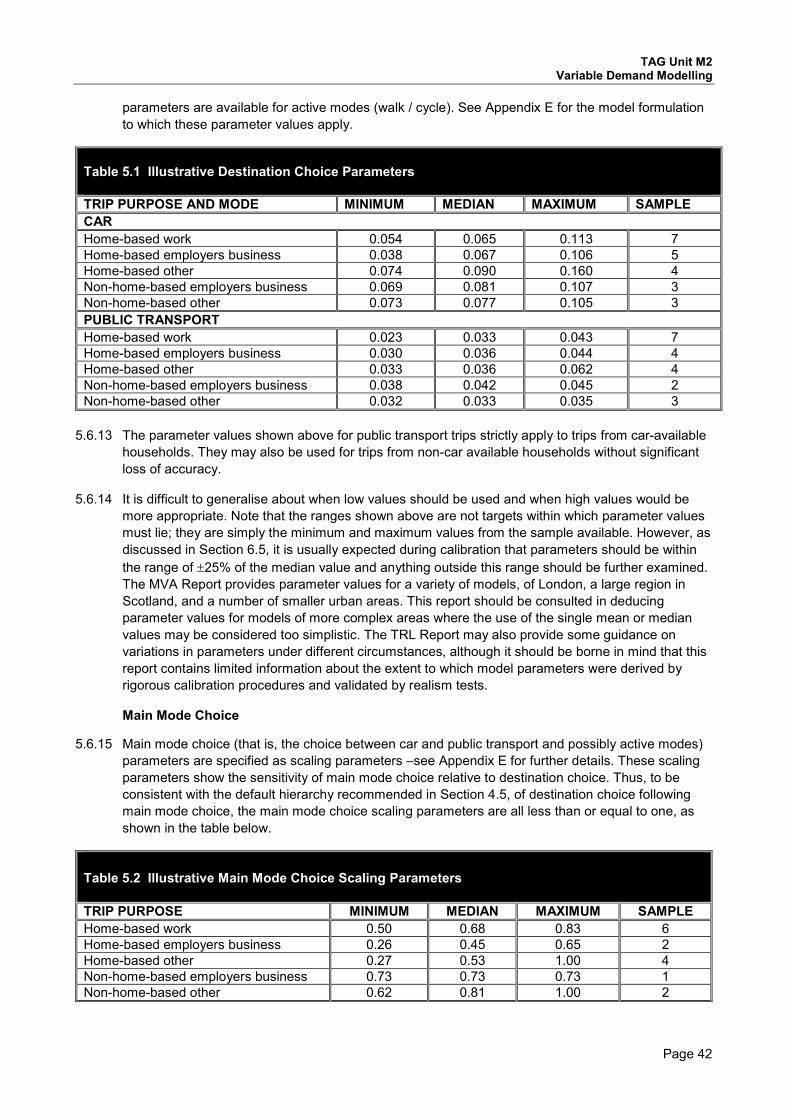
TAG Unit M2 Variable Demand Modelling
Page 42
parameters are available for active modes (walk / cycle). See Appendix E for the model formulation to which these parameter values apply.
Table 5.1 Illustrative Destination Choice Parameters TRIP PURPOSE AND MODE MINIMUM MEDIAN MAXIMUM SAMPLE CAR Home-based work 0.054 0.065 0.113 7 Home-based employers business 0.038 0.067 0.106 5 Home-based other 0.074 0.090 0.160 4 Non-home-based employers business 0.069 0.081 0.107 3 Non-home-based other 0.073 0.077 0.105 3 PUBLIC TRANSPORT Home-based work 0.023 0.033 0.043 7 Home-based employers business 0.030 0.036 0.044 4 Home-based other 0.033 0.036 0.062 4 Non-home-based employers business 0.038 0.042 0.045 2 Non-home-based other 0.032 0.033 0.035 3
5.6.13 The parameter values shown above for public transport trips strictly apply to trips from car-available
households. They may also be used for trips from non-car available households without significant loss of accuracy.
5.6.14 It is difficult to generalise about when low values should be used and when high values would be more appropriate. Note that the ranges shown above are not targets within which parameter values must lie; they are simply the minimum and maximum values from the sample available. However, as discussed in Section 6.5, it is usually expected during calibration that parameters should be within the range of ±25% of the median value and anything outside this range should be further examined. The MVA Report provides parameter values for a variety of models, of London, a large region in Scotland, and a number of smaller urban areas. This report should be consulted in deducing parameter values for models of more complex areas where the use of the single mean or median values may be considered too simplistic. The TRL Report may also provide some guidance on variations in parameters under different circumstances, although it should be borne in mind that this report contains limited information about the extent to which model parameters were derived by rigorous calibration procedures and validated by realism tests.
Main Mode Choice
5.6.15 Main mode choice (that is, the choice between car and public transport and possibly active modes) parameters are specified as scaling parameters –see Appendix E for further details. These scaling parameters show the sensitivity of main mode choice relative to destination choice. Thus, to be consistent with the default hierarchy recommended in Section 4.5, of destination choice following main mode choice, the main mode choice scaling parameters are all less than or equal to one, as shown in the table below.
Table 5.2 Illustrative Main Mode Choice Scaling Parameters TRIP PURPOSE MINIMUM MEDIAN MAXIMUM SAMPLE Home-based work 0.50 0.68 0.83 6 Home-based employers business 0.26 0.45 0.65 2 Home-based other 0.27 0.53 1.00 4 Non-home-based employers business 0.73 0.73 0.73 1 Non-home-based other 0.62 0.81 1.00 2

TAG Unit M2 Variable Demand Modelling
Page 43
5.6.16 Again, it is difficult to generalise about when low values should be used and when high values would be more appropriate. (Note that the ranges shown above are not targets within which parameter values must lie; they are simply the minimum and maximum values from the sample available.) The MVA Report should be consulted in deducing parameter values for models of more complex areas where the use of the single mean or median values may be considered too simplistic. The TRL Report may again be of some use, noting the caveat in paragraph 5.6.2.
Time of Day Choice
5.6.17 Section 4.8 discusses that limited evidence broadly suggests that the sensitivity of macro time period choice at relatively long periods (e.g. 3 hours) should be about the same as main mode choice and hence comparable to the values in Table 5.2. Micro time period choice will clearly be more sensitive.

TAG Unit M2 Variable Demand Modelling
Page 44
6 Convergence, Realism and Sensitivity
6.1 Background
6.1.1 Once the model has been scoped and developed, it is important to ensure that the model converges, is realistic and that sufficient sensitivity tests have been undertaken in order to further validate its fitness for purpose and to understand the operation of the model before applying it directly to scheme appraisal or testing strategies.
6.2 Building the Model and Model Interfaces
6.2.1 Practitioners should use their judgment to decide on a modelling approach that best suits their needs and the scope of the model that is to be developed. Various commercial software packages are available, along with required interfaces between assignment and demand models.
6.2.2 The Department’s DIADEM software (Dynamic Integrated Assignment and DEmand Modelling) has been developed to provide simple multi-stage demand models and an interface direct with some commercially available assignment modelling packages (at present, SATURN and CONTRAM), although the interface is flexible enough that it has been used with other packages. DIADEM contains procedures that apply a range of convergence improving techniques, guided by a number of convergence measures and desired stop criteria. For further information, see Appendix H.
6.2.3 There are a number of different approaches that can be adopted in developing assignment and demand models and their interfaces that are crucial when considering general performance and convergence issues:
Combined Assignment-Demand Models
6.2.4 Some software packages can handle demand-supply responses as a combined assignment-demand model. This is the preferred solution in most cases since the software will be constructed to ensure, as far as possible, that the model is properly integrated, computationally efficient and sufficiently converged to a correct solution. At present the main drawback is that the demand responses that can be modelled may be limited, either in number or in the sequence order; or the embedded assignment model does not provide all the functionality required for the area, e.g. detailed junction modelling.
6.2.5 With some models, more exact measures of convergence can be defined than the % relative GAP measure recommended in Section 6.3. This may arise from the nature of the combined demand-supply formulation. The approach to improve convergence should be given in the Validation Report. The TUBA tests outlined in Section 6.3 can be done to ensure that convergence is to the level required by the scale of the scheme.
Combining Separate Demand and Assignment Models
6.2.6 The next best alternative is to make use of a transportation software suite’s matrix manipulation tools to construct an interface and iterate between the assignment program and the demand model. This will ensure that the supply and demand data are in compatible format. Various transportation software packages are available that cover both demand and assignment functions.
6.2.7 The user will need to ensure that the final solution meets the convergence criteria set out in Section 6.3. This requires the demand model and assignment model to be run alternately, usually with the cost matrix being passed directly from the assignment model to the demand model. The trip matrix may be passed directly from the demand model to the assignment model, but this approach may require a large number of iterations, a potentially unacceptable amount of time to run, and is not guaranteed to converge. Other algorithms (e.g. the Method of Successive Averages (MSA)) combine a proportion of the demand matrix with demand matrices from earlier iterations, and may reach the convergence criteria more quickly.

TAG Unit M2 Variable Demand Modelling
Page 45
6.2.8 It is difficult to provide a single ready-made solution for all software and all schemes, and it may be necessary to seek advice from the software developers. For these models the iteration between assignment model and demand models should give statistics from which to calculate the % GAP statistic, as recommended in Section 6.3. The approach to iterating between the supply and demand models, and the monitoring of the convergence progress should be detailed in the Validation Report. Evidence should be provided that the models meet the convergence requirements set out in Paragraph 6.3.10.
6.3 Convergence
6.3.1 It is of crucial importance to demonstrate that the whole model system converges to a satisfactory degree, in order to have confidence that the model results are as free from error and ‘noise’ as possible.
6.3.2 Convergence of the full model system, i.e. iteration between demand and supply, or in other words between the demand response components and (public transport and highway) assignment, may be monitored using the guidelines developed for DIADEM; if necessary the convergence algorithms designed in DIADEM, or indeed any other appropriate software, could be incorporated in the model system to aid in achieving required levels of convergence..
6.3.3 Preliminary tests indicate that improved demand convergence can reduce the convergence errors to less than 10% of the economic benefit derived from the intervention. Demand modelling software may provide a number of measures of convergence, both relating to proximity (how close to the true equilibrium), and stability (how much the results are changing each iteration). For the purposes of this Unit, the proximity measures are the more important.
6.3.4 The recommended criterion for measuring convergence between demand and supply models is the demand/supply gap defined by:
100*)(
))(()(
∑
∑ −
an
an
a
an
an
an
a
XXC
XXCDXC
where:
naX is cell a in the previous assignment matrix for iteration n;
( )naXC is cell a in the generalised costs resulting from assigning that matrix
))(( naXCD is cell a in the matrix output by the demand model based on costs ( )n
aXC . In models where the matrix output by the demand model is used directly as the assignment matrix (as will
usually be the case in variable demand models), this will be equal to 1+naX 13.
a represents every combination of origin, destination, demand segment/user class, time period and mode
6.3.5 This is a measure of how far the current flow is from the equilibrium point and will be zero in a perfectly converged model. The demand-supply gap is represented, for one flow, by the shaded area in Figure 6.1. As convergence improves, and the difference in trips between successive iterations decreases so the shaded area decreases until the equilibrium point is reached. One of the reasons for the choice of this statistic is that it is easily calculated and is not dependant on the
13 Convergence is being measured according to whether the weighted demand (or cost) is different from what would be obtained in the next iteration if no further weighting occurred. Unless the cobweb approach is being used, it is incorrect to treat D(C(Xan)) as Xan+1. This may give a misleading impression of convergence.

TAG Unit M2 Variable Demand Modelling
Page 46
precise form of demand-supply modelling undertaken. It is referred to as the %GAP, reflecting its relative nature.
Figure 6.1 Measuring Convergence between Demand and Supply
6.3.6 The demand/supply model used may report other measures of convergence. Some of these may be stability statistics that indicate how much the solution is changing from one iteration to the next. An example of this could be the maximum change in absolute flows. It is often assumed that a stable solution implies convergence. However, it can also be an artefact of the particular algorithm being used so stability statistics are, in general, not a good indicator of how close the solution is to equilibrium.
6.3.7 It is beneficial to monitor and report the %GAP for not only the last iteration of demand and supply, but for several iterations in order to understand the stability of the model.
6.3.8 Tests indicate that gap values of less than 0.1% can be achieved in many cases, although in more problematic systems this may be nearer to 0.2%. Where the convergence level, as measured by the %GAP, is over 0.2% remedial steps should be taken to improve the convergence, by increasing the assignment accuracy.
6.3.9 To optimise processing time and help reach converged solutions the travel cost formulations used in both assignment and demand models should contain a ratio of weights of journey time relative to journey distance that are as consistent as possible. Where possible, it will be beneficial to have available an integrated and automated demand and assignment process.
Convergence and scheme benefits
6.3.10 The required level of convergence needs to be linked to the scale of the benefits of the scheme being appraised, relative to the network size. For instance the calculation of benefits from small schemes in large networks will be much more sensitive to convergence than large schemes in small networks. On the basis of testing it has been discovered that the following rule of thumb may be a useful indicator of the suitability of the convergence of the model: ideally the user benefits, as a percentage of network costs, should be at least 10 times the % Gap achieved in the Without-Scheme and With-Scheme scenarios.
6.3.11 User benefits can be derived through use of DfT’s TUBA software. It may also be done manually by using matrix manipulation of the with and without scheme trip and skimmed generalised cost matrices to produce an estimate of the consumer surplus by the rule of a half.
Cost
Trips
D
X
C(X)
D(C(X))
Cost
Trips
D
X
C(X)
D(C(X))

TAG Unit M2 Variable Demand Modelling
Page 47
6.4 Realism Testing
6.4.1 Once a variable demand model has been constructed, it is essential to ensure that it behaves ‘realistically’, by changing the various components of travel costs and times and checking that the overall demand response accords with general experience. If it does not, then the values of the parameters controlling the response of demand to costs should be adjusted until an acceptable response is achieved. There will be more scope for adjustments to model parameters where they have been imported and where the model form is incremental, and less scope where the model parameters have been estimated from local data and/or where the model form is absolute. Ways of adjusting models to improve the outcome of the realism tests are discussed in Section 6.5.
6.4.2 In this section, the calculations required for the realism tests are defined. Advice is also provided on how the acceptability of the test results may be judged.
6.4.3 Many of the parameters controlling the behaviour of a model ought to reflect local circumstances. However, even if there are adequate local data for an acceptable estimation or calibration of a model, the fact that a model replicates the travel patterns in base year cross-sectional data satisfactorily does not guarantee that the model is a good predictor of the demand responses to changes in travel costs over time and responses to changes in travel costs brought about by schemes in the forecast year. Also, in cases where a local estimation or calibration is not possible and parameter values are imported from other models or from the illustrative values provided in Section 5.6, it will be important to check that the behaviour resulting from these parameter values is plausible in their new context.
6.4.4 If the model does not behave in accordance with general experience, it should not be used to appraise a transport scheme, unless a convincing case can be made to explain the differences in terms of special local circumstances. Instead, the model parameters should be modified until its responses are plausible (as advised in Section 6.5).
Demand Elasticities
6.4.5 The acceptability of the model’s responses is determined by its demand elasticities. These demand elasticities are calculated by changing a cost or time component by a small global proportionate amount and calculating the proportionate change in travel made. These changes may be implemented on either a link basis and skimmed to yield the interzonal changes or directly at the matrix cell level. The elasticity recommended is:
e = (log(T1)-log(T0))/(log(C1)-log(C0)),
where the superscripts 0 and 1 indicate values of demand, T, and cost, C, before and after the change in cost, respectively. For example, if car fuel costs increase by 10% and trips by car fall by 2%, then the elasticity of car trips with respect to fuel cost would be log(0.98)/log(1.10)=-0.212. For the purposes of these realism tests, demand would be in terms of vehicle-kms14 (for private modes) or person trips (for public transport). Elasticities would normally represent long-term responses unless indicated otherwise.
The Tests Required
6.4.6 Any component of cost or travel time can be used to calculate demand elasticities; however, they are not all independent so that there may be little point in checking all of them separately. The different components of generalised cost for any particular journey are interlinked by the weights applied in calculating the generalised cost (see Section 3). Thus, if one weighted component always accounts for twice as much as another in the total cost, the elasticity of demand relative to it will always be twice as much. Nevertheless, it is desirable to test the more important components in this way to ensure that the formulation of generalised cost in the model is correct.
14 An exception to this is car journey time, which uses trips.

TAG Unit M2 Variable Demand Modelling
Page 48
6.4.7 The primary realism tests require that car fuel cost and public transport fare elasticities lie within specified bands (as set out below). Car fuel cost elasticity tests are required in all cases where a highway model is used. Public transport fare elasticity tests are required in all cases where changes in public transport generalised costs, including changes in fares, are modelled. Car journey time elasticity tests are also required (as a potentially useful diagnostic). Other realism tests – for example, of a model’s ability to reproduce elasticities of demand with respect to other charges, such as parking charges and tolls - may be appropriate where empirical elasticities are available.
6.4.8 The elasticities should be calculated using the base year model.
6.4.9 In order to achieve acceptable results from these realism tests, it may be necessary to modify or damp the generalised cost changes used in the demand model for longer trips. The mechanisms by which cost damping may be implemented are specified in Section 3.3. In models where the parameter values are estimated or calibrated from local data, cost damping, if it is to be employed, should be built in to the model at the estimation or calibration stage. In these cases, the realism tests should always include the cost damping. In models where parameter values are imported, initial realism tests may be undertaken without cost damping to gain an understanding of the impact of cost damping if and when it is introduced15. Advice on the introduction of cost damping is provided in Section 6.5.
6.4.10 The elasticities should be calculated from a converged run of the demand/supply loop. This requirement arises from the fact that these observed elasticities, against which the modelled elasticities are to be compared, are the result of the real world interaction of demand responses, congestion and crowding. Running a model to full equilibrium may be time-consuming and it may be more practical to explore the sensitivity of the demand elasticities to changes in the model parameter values using fewer iterations. If this approach is adopted, the extent to which the elasticities resulting from the smaller number of iterations are changed by further iteration to convergence should be established at the outset.
6.4.11 A demand weighted average of these elasticities by time period and demand segment or user class should be taken so that the result ideally represents the average elasticity for the whole year, including weekends and holidays. This is because the target elasticity specified below relates to all periods of the year. The annualisation factors used for the Transport Economic Efficiency appraisal may be used for this purpose – see TAG Unit A1.3. Where the annualisation factors do not account for all periods of the year, the available factors should be used but their limitations should be noted in the realism test reporting.
Car Fuel Cost Elasticity
6.4.12 The car fuel cost elasticity required is the percentage change in car vehicle-kms with respect to the percentage change in fuel cost. The calculations should be carried out for a 10% or a 20% fuel cost increase. (A 10% increase is preferred but, in some cases, a larger increase, such as 20% has proved necessary for plausible results to be obtained.) Care should be taken not to increase non-fuel operating costs in this process.
6.4.13 Car fuel cost elasticities should be calculated in both of the following ways.
• Matrix-based
• The change in car vehicle-kms should be calculated from the car trip matrices and skimmed distance matrices which relate to the before and after fuel cost change model
15 This will be the case where the illustrative parameters in Section 5.6 are used, or if the model from which the parameters are imported has no cost damping. Where parameters have been imported from a model that employed cost damping, that function should be imported also and tested to see if realism tests are met. If this fails, the model will need to be re-estimated or calibrated by adjusting the behavioural parameters, ASCs and/or the cost damping function (see Section 6.5).

TAG Unit M2 Variable Demand Modelling
Page 49
runs. The movements included in this calculation should relate only to the movements to which the full range of demand responses apply in the demand model.
• For example, if external to external trips are treated as fixed, then it could be argued that the responses of external to internal trips would not be fully responsive as the model would not allow change of destination so that external to internal trips became external to external and vice versa. In this case, the matrix-based calculations should use only the internal to external and internal to internal trips.
• Even if external to external trips are not fixed, they will very often be modelled in a very approximate manner using very simplified networks and speed/flow relationships and approximate estimates of demand. In all such cases, external to external movements should be excluded from the elasticity calculations.
• Complete trips, from real origin to real destination, should be used for these elasticity calculations. This can often require a zoning system and network which covers a large area. These calculations should be carried out by time period and car trip purpose, and also aggregated over time periods and trip purposes to produce an overall average elasticity.
• The calculations can be carried out on either an O/D or P/A basis, although the former is likely to be the more convenient.
• Network-based
• Car vehicle-kms should be accumulated over a specified network from the before and after fuel cost change runs and the difference taken. The network used for this calculation should extend to cover the area over which the highway assignment model has been validated but should exclude external areas where the model is more approximate.
• This calculation is likely to underestimate the fuel cost elasticity if the change in car-kms includes fixed elements, such as external to external trips (unless the external to external car-kms can be excluded from the calculations). These calculations should be carried out by time period and car user class, and also aggregated over time periods and trip purposes to produce an overall average elasticity.
6.4.14 A number of UK studies using time-series data on car travel and fuel prices and costs have shown an elasticity of car use with respect to fuel cost of about -0.3 (see Bradburn and Hyman (2002), Graham and Glaister (2002), Hanly, Dargay and Goodwin (2002)) and this value equates well with a review of European research on this topic (TRACE, 1999). Taking account of this research, unless analysts can provide a good reason otherwise, the Department’s view is that:
• the annual average fuel cost elasticity should lie within the range -0.25 to -0.35 (overall, across all purposes); and
• the annual average fuel cost elasticity should lie on the right side of -0.3, taking account of the levels of income and average trip lengths prevailing in the modelled area – see below for advice on what is the ‘right’ side of -0.3.
6.4.15 Fuel cost elasticities would be expected to be weaker than -0.3 (i.e. closer to zero) where trip lengths are shorter than average, car driver mode shares are higher than average, and where proportions of low elasticity demand segments, such as employers’ business, are higher than average, and stronger (i.e. further from zero) where the opposite applies. Higher than average income levels may also be consistent with a weaker elasticity. However, it is generally difficult to estimate the magnitude of the effects of these factors and therefore the extent to which the true elasticity for the area being modelled may vary from the figure of -0.3. It is for this reason that an acceptable range, from -0.25 to -0.35, is specified and analysts should not use models for scheme

TAG Unit M2 Variable Demand Modelling
Page 50
appraisal which have elasticities outside this range without providing a reasoned case for doing so and without the Department’s approval.
6.4.16 Note that, if local variations in values of time are used to argue for a particular target fuel cost elasticity, local values of time should be used in the model. In this case, evidence for the local values of time will be required.
6.4.17 Elasticities may also be regarded as more plausible if:
• the pattern of annual average elasticities shows values for employers’ business trips near to -0.1, for discretionary trips near to -0.4, and for commuting and education somewhere near the average; and
• the pattern of all-purpose elasticities shows peak period elasticities which are lower than inter-peak elasticities which are lower than off-peak elasticities.
6.4.18 While there is little or no empirical evidence to support the variation in elasticities by purpose and time period, most models show the pattern suggested above, although a few models which are otherwise acceptable have been created which show morning peak elasticities which are higher than inter-peak elasticities which are higher than evening peak elasticities. In the case of models which show different variations in elasticities by purpose and time period, an explanation for the differences will need to be provided.
Public Transport Main Mode Fare Elasticities
6.4.19 The public transport fare elasticity required is the percentage change in public transport trips by all public transport modes with respect to the percentage change in public transport fares. The calculations should be carried out for a 10% or a 20% public transport fare increase, applied to all public transport modes equally.
6.4.20 Public transport fare elasticities should be calculated on a matrix basis, by time period and trip purpose. The movements included in this calculation should relate only to the movements to which the full range of demand responses apply in the demand model and should generally exclude external to external movements in any event. Complete trips, from real origin to real destination, should be used for these elasticity calculations.
6.4.21 Elasticities of public transport trips with respect to public transport fares have been found to lie typically in the range –0.2 to -0.9 for changes over a period longer than a year (TRL, 2004). Values close to -0.2 are unlikely for the whole public transport market unless this includes a high proportion of concessionary fare trips with a significant number made free of charge.
6.4.22 The elasticities may also be regarded as more plausible if:
• the pattern of annual average public transport fare elasticities shows values for non-discretionary purposes which are lower than those for discretionary trips; and
• the pattern of all-purpose public transport fare elasticities shows peak period elasticities which are lower than inter-peak elasticities which are lower than off-peak elasticities; and
• the elasticities for car-available segments are greater than the non-car-available segments since the former have greater choice than the latter, although there are arguments to suggest that non-car-available fare elasticities may be higher where incomes are lower.
However, there is little or no empirical evidence available to support these patterns and other patterns may be acceptable.
TAG Unit M2 Variable Demand Modelling
Page 51
Public Transport Sub-modes
6.4.23 In addition to calculating elasticities for all public transport trips combined, separate elasticities should be calculated for all public transport sub-modes which carry significant shares, where the model structure allows such calculations to be undertaken in an appropriate manner. In order for valid fare elasticities for individual public transport sub-modes to be calculated, the fares applicable to the sub-mode would need to be explicitly included in the generalised costs used in the model. In the case of models where the split between the public transport sub-models is handled in the public transport assignment model, fares for each sub-mode would need to be included in both the demand model and the public transport assignment model. Where this is handled in the demand model, fares by each sub-mode would need to be included in the costs used in that choice process (but would not be needed in the assignments which would be restricted in each case to a single sub-mode).
6.4.24 Elasticities of bus trips with respect to bus fares for full fare paying passengers have been found to lie typically in the range –0.7 to -0.9 for changes over a period longer than 5 years (Dargay and Hanley). Unless analysts can provide a good reason otherwise, the Department’s view is that the annual average bus fare elasticity from the base year model should lie within this range. It should be noted that up to a third of bus trips made in the off-peak and some in the morning peak are made by concessionary passengers free of charge. Their demand will be unaffected by changes in fares. If possible, it would be useful to estimate the fare elasticity for full fare paying passengers separately noting that there are several half-fare or similar schemes for children and students. Including concessionary passengers would tend to reduce the elasticities given above to around -0.4 with a lower elasticity in the off-peak. There is no available evidence of the long-run fare elasticities for heavy and light rail.
Short and Long-Term Trip Kilometre Elasticities
6.4.25 The range of trip-kilometre elasticities shown in Table 6.1 have been used to validate a number of multi-modal models and may also be useful in addition to the elasticities given in this Section.
Table 6.1 Expected Short and Long-Term Trip Kilometre Elasticities High Central Low Car fuel (cost/km after allowing for vehicle fuel efficiency changes) 1 year -0.28 -0.125 -0.07 5 years -0.32 -0.2 -0.13 10 years or longer -0.48 -0.3 -0.19 Bus fares 1 year -0.65 -0.3 -0.16 5 years -0.96 -0.6 -0.38 10 years or longer -1.12 -0.7 -0.44
Car Journey Time Elasticity
6.4.26 The car journey time elasticity required is the change in car trips with respect to the change in journey time (calculated using the formulation given in 6.4.5).
6.4.27 These journey time elasticities should be calculated using a single run of the demand model because the target elasticities in this case were derived from stated preference data, where the costs of each option and attribute were exogenous.
6.4.28 Journey time elasticities should be calculated from both a model run and on a matrix-basis using times from the networks, for each trip purpose in each time period. Complete trips, from real origin to real destination, should be used for these elasticity calculations. The output elasticities should be

TAG Unit M2 Variable Demand Modelling
Page 52
checked to ensure that the model does not produce very high output elasticities (say stronger than -2.0).
Summary of Recommended Elasticities
6.4.29 Table 6.2 below summarises the recommended elasticities that should be achieved by the realism tests outlined in this Section.
Table 6.2 Summary of Recommended Elasticity Ranges High Low Average Fuel Cost (kms) -0.35 -0.25 PT Main Mode Fare (trips) -0.9 -0.2 Bus Fare (trips) -0.9 -0.7 Car Journey Time (trips) No stronger than -2.0
6.5 Model Adjustment
6.5.1 This section explains what should be done if a model fails to yield elasticities in the specified ranges and adjustment to the model is deemed necessary.
6.5.2 The model is required to satisfy expected car fuel cost, car journey time and public transport fare elasticities and trip lengths for each mode. Where it does not, the following main model features may be adjusted in order to do so:
• the model sensitivity parameters;
• the values of time; and
• the cost damping function.
6.5.3 These features are considered in turn, for each of two kinds of model:
• first, models which have been developed by importing sensitivity parameter values from either an existing model whose parameters have been estimated16 statistically reliably; and
• secondly, models for which parameter values, and possibly values of time also, have been estimated statistically from local data.
Models Developed by Importing Initial Parameter Values
6.5.4 Elasticities. As noted in Section 6.4, for models with imported parameters, initial realism tests may be undertaken without cost damping to gain an understanding of the impact of cost damping if and when it is introduced17.
6.5.5 Sensitivity Parameters. The data base used to derive the illustrative lambda and theta demand parameter is described in Section 5.6. Notwithstanding the associated caveats, the Department considers that analysts should start with the median lambdas and thetas and adopt a cautious, simple and systematic process for modifying these. In general, care should be taken to avoid over-complicating the adjustments to the median lambdas and thetas.
6.5.6 A record of all the changes made and their results should be kept and made available if requested. The aim should be to reduce the chances of peculiar combinations being selected for no good
16 In this context, ‘estimation’ is a statistical process and ‘calibration’ is a process of adjustment, often by trial and error. Thus, demand model parameters are often ‘estimated’ while assignment models are often ‘calibrated’. 17 Assuming that the model parameters being imported from itself does not have cost damping, as discussed in Section 6.4.

TAG Unit M2 Variable Demand Modelling
Page 53
reason. Consistency in matters like this helps the Department interpret appraisals and check results for plausibility. Typically, revised lambdas and thetas which were within +25% of the median illustrative values would be regarded as acceptable and values outside this range would merit investigation.
6.5.7 Values of Time. Varying the value of time with distance is one of the recommended forms of cost damping and is considered separately, below. The advice here is concerned with the notion of changes to the average values of time, irrespective of distance.
6.5.8 It is strongly advised that the generalised costs used in both assignment and demand models are compatible18 and that values of time and vehicle operating costs given in TAG Data Book should be used19.
6.5.9 If values of time are changed in order to achieve better elasticities, a revalidation, and possibly a recalibration also, of the assignment model would also be required. If the values in the assignment model were left unchanged and were only changed in the demand model, an inconsistency would arise between the values used in the demand and assignment models. Consistency must be assured18.
6.5.10 Given these considerations, analysts should:
• start with WebTAG values of time unless they can put forward good reasons for doing otherwise; and
• start with compatible generalised cost coefficients (vehicle operating costs and values of time) in the assignment and demand models.
6.5.11 That said, it is allowable to estimate values of time which differ from the WebTAG values (see TAG Unit M4, for example). Thus, analysts may adjust the starting WebTAG values of time to achieve better elasticities, but only if they have good evidence from estimation using either revealed or stated preference data that show local values of time that are different from the equity values presented in the TAG Data Book. A strong justification must be made for changes to the WebTAG average values of time in excess of +20%.
6.5.12 Cost Damping Function. If cost damping is to be employed, the following forms or functions are recommended:
• variation in the value of time with distance; and/or,
• damping of generalised cost by either a function of distance or a power function; and/or,
• use of a log cost term along with the conventional linear cost term in the generalised cost function.
6.5.13 For the damping of generalised cost by either a function of distance or a power function, there are parameters that can be adjusted by the analyst. The cost damping functions given in Section 3.3 effectively scale the generalised costs. In principle, therefore, the functions and suggested parameter values apply equally to trip-based and tour-based models, although, in practice, parameter values may need to vary according to local characteristics.
6.5.14 Trip Lengths. If the model is a true incremental model and has been set up by initially importing parameter values, checks on how well the final parameter values reproduce observed trip lengths
18 Except to the extent that certain elements of generalised cost may be relevant to only one of the models and that the costs should relate to vehicles in the assignment model and persons in the demand model. 19 The advice in DMRB Volume 12 allows the analyst to adjust the value of time in an assignment model but then advises that the resulting distance coefficient should be held constant in forecasting. This approach causes inconsistencies with the demand model where vehicle operating costs and values of time are normally changed over time in forecasting and hence is not recommended where a variable demand model is used.
TAG Unit M2 Variable Demand Modelling
Page 54
are not required. However, if the model is an absolute model, whether used in absolute form or applied incrementally, then checks should be made to assess how well the model parameters reproduce observed trip lengths.
6.5.15 In summary: in the case of models which have been developed by importing sensitivity parameter values, there is scope to achieve more acceptable elasticities by:
• adjusting the sensitivity parameters within a defined range; and
• using a form of cost damping and adjusting the parameters which define that function.
Models for Which Parameter Values, and Possibly Values of Time, Have Been Calibrated
6.5.16 Elasticities. The target elasticities and their ranges are not affected by how the model has been developed and therefore apply to this category of models too.
6.5.17 Sensitivity Parameters. In this category of models, sensitivity parameters and Alternative-Specific Constants (ASCs) will have been estimated to reproduce observed trip lengths for each demand segment (as well as observed trip patterns and volumes). In some cases, it may be possible to adjust the sensitivity parameters to yield more appropriate elasticities while maintaining the fit to the observed trip length distributions by means of adjustments to the ASCs. However, in most cases, this could be a complicated and arguably impractical process. Therefore, the scope for adjusting estimated sensitivity parameters is probably quite limited (although revised parameters may arise from some of the other adjustments below).
6.5.18 Values of Time. If values of time have been taken from WebTAG initially, they may be adjusted only if an estimation using local revealed or stated preference data supports the change. If changes to the initial values of time are made on these grounds, the sensitivity parameters and ASCs would need to be re-estimated.
6.5.19 In some cases, values of time are estimated as part of the model estimation process. Once these have been accepted as plausible, it would be very hard to find good reason to adjust them in order to achieve more acceptable elasticities.
6.5.20 Cost Damping. In principle, the same range of cost damping forms is available for use in this category of models as in the models which started with imported parameters. However, in this case, these functions must be employed at the stage before sensitivity parameters and ASCs, and values of time, are estimated. Cost damping cannot be retro-fitted without re-estimation.
6.5.21 It is open to the analyst to adjust the parameters which define the cost damping function, with the same scope for adjustment being available as for the models which start with imported sensitivity parameters. These adjustments may be carried out initially without re-estimating the model but, once a favoured set of cost damping parameters has emerged, the sensitivity parameters, ASCs and values of time, must be re-estimated.
6.5.22 It is possible that there will be a number of combinations of cost damping parameters, choice model sensitivity parameters, and ASCs that would yield an acceptable model. Calibration should focus on achieving the most suitable sensitivity parameters and ASCs before attempting to adjust the cost damping function to achieve better model fit.
6.5.23 Trip Lengths. The statistical estimation processes are designed to identify sensitivity parameters, ASCs and values of time which mean that the model should replicate observed trip lengths. It may be necessary to allow some flexibility in the estimation in order that the requirements of the realism tests may be met. It may be that some relaxation of the fit of the model to the data is required, perhaps by altering the explanatory power of the sensitivity parameters and the ASCs, for the realism test requirements to be satisfied.
TAG Unit M2 Variable Demand Modelling
Page 55
6.5.24 In summary: in the case of models for which parameter values, and possibly values of time also, have been estimated from local data, there should be scope to achieve more acceptable elasticities by:
• adjusting the sensitivity parameters and ASCs; and
• using a form of cost damping and adjusting the parameters that define that function.
6.5.25 The practicality of adjusting the sensitivity parameters and ASCs may be restricted, as may be the scale of any changes that could be made by these means. If it is decided that cost damping should be introduced (not having been included in the initial estimation), the model would have to be re-estimated with the chosen cost damping function and parameters.
6.6 Sensitivity Testing
6.6.1 Sensitivity testing, as distinct from realism testing, is aimed at identifying the relative effects of the various parameters on the outcome of a scheme appraisal, rather than in checking the model responses against experience. Especially where the model parameter values are uncertain, it is important to know how sensitive the appraisal results are to these uncertainties, so that confidence can be invested in the conclusions.
6.6.2 Sensitivity testing should be undertaken of the model’s behaviour against variation in those parameters that are judged to:
• have a substantial effect on the model’s prediction of changes when forecasting, and
• be uncertain in their calibration.
6.6.3 The most obvious values are the sensitivity parameters that govern the individual demand mechanisms (i.e. the lambda values). If they have been calibrated on local data, the extent of possible error in their calibration should be examined from the statistics calculated during the fitting, which is usually substantial. If they have been imported, the uncertainty may be even greater since they are being used in a context different from their original application. The illustrative values given in Section 5.6 were obtained from a review of models of a generally acceptable form available at the time for which parameters had been estimated; and typically the range of values was twice the mean value. This indicates the degree of uncertainty in values imported from other studies.
6.6.4 If the lambda values have been calibrated on local data, whether for the variable demand model itself or for an existing local model, then check the overall result of the scheme appraisal against runs of the model with the lambdas set at +25% of the mean, or +1 s.d., whichever is larger. Behaviour of the model will not necessarily be symmetrical against increases and decreases in the parameter, but the increase will indicate the strength of the response, and if it is an important factor the result can also be tested against a decrease. If the values have been imported then test the result against +50% of the mean. This range is to reflect the greater uncertainty that occurs with imported values. Unless there are convincing reasons for not doing so, the changes are to be made to all parameters in the same direction at the same time so that the gradation of parameter values is still consistent with the hierarchy.
6.6.5 Given the acknowledged uncertainty of distribution parameters obtained from cross-sectional fitting, this larger margin could be applied even to locally calibrated distribution lambdas. It is the stronger variable demand mechanisms which will have most effect on the assessment, so there may be no point in testing the result against a small trip frequency response, for example, when distribution or mode choice are dominant.
6.6.6 Where the model includes time of day choice it will be essential to test variation of the assumed sensitivity. Evidence for these values is more uncertain and wide sensitivity factors say: +50% and -50% of the mean are suggested. The range will be limited by the need to ensure that any changes in the values are still consistent with the hierarchy.

TAG Unit M2 Variable Demand Modelling
Page 56
6.6.7 Sensitivity testing should not be limited to the response parameters, however. Any parameter that seems likely to have a substantial effect on the net benefit, and where appreciable uncertainty is likely to affect the assessment substantially, should also be tested. An example of this may be the assumed distribution of willingness-to-pay bands in road-tolling exercises.
6.6.8 Although sensitivity testing is important, there is a danger in using it to obtain such a wide range of values that any prediction is mistrusted. In interpreting the results it is important to understand (and to emphasise in presentation) that the central values are still the best available prediction of the likely outcome and additional forecasts obtained by sensitivity testing are purely to establish the effects of uncertainty around this central forecast. The aim is for the modeller to make clear the extent of the possible uncertainty, while providing clear central predictions to support policy making and assessment.
6.6.9 There are other sensitivity tests that should be undertaken for forecast years to test the sensitivity of the appraisal to variations in other inputs such as changes in the build-up of demand, values of time, or differing economic forecasts. These tests are described in more detail in TAG Unit M4 – Forecasting and Uncertainty.
6.7 Reporting
6.7.1 The results of the realism tests should be documented in a validation report. The items that should be included in a Validation Report are set out in significant detail in DMRB Volume 12 Section 2 Part 1.
6.7.2 Particularly related to forecasting, realism and sensitivity, the report should include at least the following items:-
• The background to the decision on the particular demand responses included in the model. This will include a statement on any demand tests.
• A description of the reasoning behind the choice of lambda parameter values, including any local calibration should be given. The parameter values should be explicitly shown together with details of the elements of generalised cost, and the route-choice factors.
• Details should be given of any realism tests, which should, at least, include the estimation of the elasticity of car travel (vehicle kilometres) to changes in car fuel cost and, if possible, the elasticity of car trips to car journey time. Where a mode-choice has been included the realism checks should also include the sensitivity to changing bus/rail fares. The Report should also include details of any changes to the model parameters arising from these tests.
• Details should be given of any base year sensitivity tests undertaken and their potential implications for forecasting.

TAG Unit M2 Variable Demand Modelling
Page 57
7 References Batley R, T Fowkes, G Whelan and A Daly.(2001) Models for choice of departure time. European Transport Conference, Seminar on methodological innovations Homerton College, Cambridge Sept 2001
Bradburn, P and Hyman, G (2002). An econometric investigation of car use in the National Transport Model for Great Britain. European Transport Conference, September 2002, Seminar on Applied Transport Methods, Homerton College Cambridge 2002
Daly, A (2008), The Relationship of Cost Sensitivity and Trip Length, European Transport Conference, Transport Modelling Seminar, Leeuwenhorst, The Netherlands.
Daly, A (2010), Cost Damping in Travel Demand Models Report of a study for the Department for Transport. http://www.rand.org/pubs/technical_reports/TR717.html
Dargay J.M. & Hanley M. (1999), Bus Fare Elasticities.
Department for Transport (2015), 'Provision of market research for value of travel time savings and reliability: Phase 2 Report'. https://www.gov.uk/government/uploads/system/uploads/attachment_data/file/470231/vtts-phase-2-report-issue-august-2015.pdf
DMRB 12.2.2 HMSO February 1997 - withdrawn Summer 2004
Graham D & S Glaister (2002) Review of income and price elasticites of demand for road traffic. Final report to the DTLR. July 2002.
Hanly M, J Dargay & P Goodwin (2002) Review of Income and Price Elasticities in the Demand for Road traffic. Final Report to DTLR. March 2002.
Highways Agency (1996) Traffic Appraisal in Urban Areas (Design Manual for Roads and Bridges (DMRB) 12)
Institution of Highways and Transportation (1996) Guidelines on Developing Urban Transport Strategies.
Institute of Transport Studies, University of Leeds, in association with John Bates Services (2003), Values of travel time savings in the UK.
MVA (2005), Multi-Modal Model Data Provision.
Ortuzar, J de D and Willumsen, L G (2001). Modelling Transport (Third Edition). Wiley, Chichester
P.J. Mackie, A.S. Fowkes, M. Wardman, G. Whelan and J. Nellthorp (Institute for Transport Studies, University of Leeds) and J. Bates (John Bates Services) (2003) Value of travel time savings in the UK: summary report. ITS Leeds, January 2003 (also available on DfT web site)
Senior M L and H C W L Williams (1977) Model-based transport policy assessment. Traffic Engineering and Control, Vol 18 (9/10).
TRACE (1999). TRACE Final report, http://www.transport-research.info/Upload/Documents/200310/trace.pdf
TRL (2001), User-friendly multi-stage modelling advice, Phase 2: Modelling parameters, calibration and validation.
TRL (2004) The demand for public transport: a practical guide. TRL Report TRL593. Crowthorne UK.

TAG Unit M2 Variable Demand Modelling
Page 58
8 Document Provenance This Unit consists of restructured and edited material from the following guidance Units that existed in the previous structure at August 2013:
Preliminary Assessment Procedures (TAG Unit 3.10.1), reflecting the consultation comments received on Steps 1 to 4 of the draft Variable Demand Modelling Advice produced by TRL in June 2003. Updated in October 2009 (3.10.1c) to include new guidance on Proportionate Appraisal. Some of these changes (most notably former Section 1.5 – ‘Further Simplifications in Demand Modelling for schemes with a capital cost below £20 million’) were removed in January 2011.
Scope of the Model (TAG Unit 3.10.2), reflecting consultation comments received on the Model Scoping Stage of the draft Variable Demand Modelling Advice produced by TRL in June 2003. The section on cost damping was added in 2009.
Key Processes (TAG Unit 3.10.3), reflecting the consultation comments received on the Key Processes Stage of the draft Variable Demand Modelling Advice produced by TRL in June 2003. This was also modified in October 2009 following the release of Proportionate Appraisal Guidance in consultation.
Convergence, Realism and Sensitivity (TAG Unit 3.10.4), first released in June 2006. Section 6.4 on realism testing was revised in May 2009 and Section 6.5 on model adjustment was added at the same time.
Model Structures and Traveller Responses for Public Transport Schemes (TAG Unit 3.11.1) has been incorporated where relevant to discuss principles that are applicable across highway and PT modes in one place.
Mode Choice Models: Bespoke and Transferred (TAG Unit 3.11.3). The elements on transferring mode choice models has been added to this unit, primarily to Appendix G. The remaining guidance on bespoke mode choice models has been retained in the Supplementary Guidance section.
Modelling Road Pricing (TAG Unit 3.12.2c). Where relevant, specific information on tolls and charging schemes have been added to this Unit.
Subsequent edits have been made in May 2016 to clarify the role of cost damping to reflect the research evidence from Provision of market research for value of travel time savings and reliability: Phase 2 Report (DfT, 2015) regarding the relationship of value of time with distance.

TAG Unit M2 Variable Demand Modelling
Page 59
Appendix A Elasticity Models
A.1 Functional Forms and Parameter Values of Elasticity Models
A.1.1 Where an elasticity model is appropriate the functional form and parameter values need to be selected. The simplest functional form – an ‘own-cost’ elasticity model - assumes that changes in the demand for travel between two points can be adequately estimated purely by a function of the change in costs between the two places.
A.1.2 However, if costs do indeed change, the relationship between change in demand and change in costs can take a number of forms, but only exponential and power formulations, and a composite of the two forms (called a Tanner function), will be considered here. With a power formulation the proportionate change in trips is related to the proportionate change in costs, as shown in the equation below. With an exponential formulation, on the other hand, the proportionate change in trips is a function of the absolute change in costs.
A.1.3 For most applications the Power relationship below which is a simple own cost elasticity model due to its constant elasticity value is recommended:
A
ij
ijijijij G
GTgT
=
00 **
Where:
Tij is the forecast number of trips between zones i and j
Gij is the forecast disutility or generalised cost
gij is the forecast growth rate relative to an earlier or base year
0Tij is the number of trips in the earlier or base year
0Gij is the disutility or generalised cost in the earlier or base year
A is the elasticity, which should be negative and is the same for all trips in the same user class.
A.1.4 This is a well-behaved formulation that is simple to apply, and is base independent: that is, it is guaranteed to give the same results if forecasts are produced from one year to another directly or via an intermediate year. It assumes that a proportionate change in trips is related to a proportionate change in costs. As the parameter A is constant the implied elasticity is the same for all lengths of trip within the same user class (i.e. it is “distance neutral”).
A.1.5 This formulation can easily be set up using the matrix manipulation facilities available in modern transportation modelling suites, or in some modelling suites combined directly with the assignment process. The facility is also available within the DIADEM modelling framework.
A.1.6 An alternative formulation is the “Exponential” relationship. In this case the effective elasticity increases with increasing trip cost, and hence for study areas where there are a wide variety of trip lengths the effective elasticities could vary markedly. Thus the exponential approach should only be considered in the case where the study area is small and urban, and where a general elasticity approach is being combined with a logit choice mechanism to jointly represent the individual demand mechanisms. Most logit mechanisms in the variable demand hierarchy share this exponential function characteristic, but some have a more benign effect since trip re-distribution, for example, can be constrained to avoid changing the overall number of trips. In that case trip re-distribution in the face of changing travel costs effectively adjusts the proportions of trips of different length to compensate for the changes. Similarly mode-choice models estimate shares rather than absolute numbers.

TAG Unit M2 Variable Demand Modelling
Page 60
A.1.7 The “Exponential” formulation assumes that the proportional change in trips is a function of the absolute change in costs:
)}(*exp{** 00 ijijijijij GGBTgT −=
Where the elasticity of demand with respect to generalised cost U is B*Gij with B negative. This is an own cost elasticity that is not simple due to the elasticity not being constant.
A.1.8 These equations can be used in two ways. They can be based or pivoted on a base year, where base trips and costs are known from empirical data, and the product gij * 0Tij represents what is referred to as the Reference Case Matrix. Alternatively, the equations can be formulated to compare costs between alternatives for the same year, where the ‘earlier’ year costs and trips are derived from the other scenario.
A.1.9 Both these formulations are closely incremental in nature, allowing the number of trips in the system to change up or down. This is in contrast to most of the individual demand-response mechanisms that are set out as share formulations where the total number of trips is fixed (say by NTEM all-mode forecasts) and merely allocated to one choice or another (e.g. to different modes or destinations).
A.1.10 Whilst the formulation is relatively easy to set up, there are some issues that must be dealt with when considering the parameter values to assign to a demand segment.
A.1.11 ‘Own cost’ elastic assignment modelling in congested Urban Areas should be undertaken at a peak hour unless there are significant variations in demand, or congestions levels are high in which case the modelling should cover linked time-periods, sub-divided into time slices and sub-periods.
A.1.12 The size of the parameter value will reflect the number of responses that the elasticity formulation is acting as proxy for. For instance, if the elasticity formulation is taking the place of all responses then it will be larger than if it is acting as proxy for only one or two responses. The table below sets out the recommended starting values for the elasticity of demand with respect to journey time.
Table A1 Derived Long-Term Car Journey Time Elasticities for Different Purposes Purpose Time
elasticity – High modal competition
Time elasticity – Low modal competition
Time elasticity –
High modal competition including time-switching
Time elasticity –
Low modal competition including time switching
Trip frequency effect (only)
HB Work -0.22 -0.14 -0.48 -0.30 -0.04
Employer's Business -0.60 -0.35 -0.96 -0.55 -0.15
Essential Other -0.47 -0.26 -0.65 -0.36 -0.12
Discretionary Other -0.35 -0.20 -0.50 -0.28 -0.10
Notes: Derived from 1997 DMRB Volume 12 Section 2 Part 2 Table C2 and paragraph C13. The values are based on car journey time elasticities - equivalent generalised cost elasticities would be about 10-50% higher, depending on the value of time and average network speed. Short-term elasticities are 28%, 8% & 5% less for HBW, Employer’s Business and Discretionary purposes respectively.
A.1.13 Equivalent journey cost elasticities can be calculated from the above table by dividing the elasticities by the proportion of the total generalised cost made up of journey time. For instance, if a model assigns on the basis of generalised cost (t+kd), the appropriate time elasticity must be multiplied by a factor (1+kv) where v is the average speed in the base year in kilometres per minute if journey

TAG Unit M2 Variable Demand Modelling
Page 61
time (t) is in minutes and distance (d) is in kilometres. TAG Data Book can be used to provide the relevant factors for given combinations of purpose, forecast period and congestion level if standard values of time are being used. In practice, the generalised cost elasticities will be between 10% and 50% higher than the values shown in the table above with values at the lower end for Employer’s Business trips, urban areas and later forecast years.
A.1.14 If an exponential formulation is used then the above values will need to be subsequently divided by the mean generalised cost to give the equivalent parameter value.
A.1.15 The estimated generalised cost elasticities (and associated parameter values if an exponential model is used) may need to be adjusted so that the fuel cost elasticity estimate from the model reflects the national overall estimate of -0.3 (see Section 6.4).
A.1.16 Where possible, the trips should be split by trip purpose (and any other known major variation such as willingness to pay or movement type). If this is not possible, for instance where only a single private vehicle user class is available, then they should be split by time-period. Using the national car driver journey purpose mix for each period of the day (from NTS), the above elasticities can be converted to elasticities for all trips by time period. If local data suggests a significantly different mix of purposes by time-period, then the local proportions can be substituted for the national ones.
A.1.17 Care should be taken when dealing with intra-zonal trips. Because most assignment models do not output intra-zonal costs (since intra-zonal trips are not assigned) there may be problems with using incremental models where there are observed intra-zonal trips in the base year trip matrix. It is desirable that robust estimates of intra-zonal costs should be estimated in these instances. These could be some function of the inter-zonal costs, for example half the minimum inter-zonal costs for that zone (of course factors such as the nature of juxtaposition of other zones and the size of the zone itself are considerations). Power function elasticity models will be particularly sensitive to very small intra-zonal costs, and this is one reason why they should be avoided when this is the case.

TAG Unit M2 Variable Demand Modelling
Page 62
Appendix B An Approach to Building the Base Demand Matrix B.1.1 This extract suggesting a possible approach to base year P/A matrix building is taken from previous
TAG Unit 3.10.2 – VDM Scope of the Model. This is a developing area of research and other emergent methods are available and others have been used across different models.
B.1.2 The essence of the approach is to begin with a wholly synthetic model, which makes minimal, but reasonable, assumptions. In this way, initial P/A matrices at the required level of detail are developed. These are then treated as a “prior” that is then modified in the light of observed data, and the reliability thereof, leading to an improved version of the base matrix.
B.1.3 The initial synthetic model should start off with the all-day zonal productions and attractions implied by NTEM for each purpose (or, better, make use of the underlying car ownership and trip end functions applied to local data on population, households and employment). The matrix cells should then be filled by means of a standard gravity model that should be constrained to reproduce (at least) average trip length for the purpose (taken either from local sources or national sources such as NTS). Next, factors giving modal choice and time of day (again, available as part of the NTEM database, although local data is preferred where possible) can be applied. In this way the complete prior matrix is built up by mode and time period, distinguishing the outbound and return portions of home-based purposes.
B.1.4 The process of “introducing observed data” must then make allowance for the statistical accuracy of that data, based essentially on sampling theory (see guidance in DMRB 12.1). This could be done along the following lines. For each observed cell of the matrix (i.e. production zone, attraction zone, purpose, mode, time period as well as possibly some segmentation data relating to car availability etc), the “prior” value would be tested as to whether it lay outside of the confidence region of the observed data: if so, the prior data will need to be modified.
B.1.5 In the course of such modification, certain key features of the prior matrix may be lost: for example, the modifications may change the total productions, or the average trip length. There will therefore be a need for an iterative process which attempts to re-impose some features as “constraints”. The modification can typically be done by means of a “proportionate fitting method”. Note that, provided that purpose is available in all the observed data, this adjustment process can be carried out independently for each purpose.
B.1.6 When the adjustments have converged to a satisfactory degree and the resulting matrices have been validated, these can be taken as an acceptable P/A basis, and used as the pivot for an incremental demand model.
B.1.7 If a modified Origin-Destination (O/D) matrix for assignment purposes has already been validated, then this matrix should be used as the basis for assignment, and predicted changes in demand (after conversion from P/A to O/D) will be used to adjust this matrix.
B.1.8 If no assignment matrix is in existence, then the first step should be to see whether the derived base P/A matrix can, when converted to O/D form, be satisfactorily validated at the assignment level. However, problems may be incurred when, after reasonable adjustments to the network, it is concluded that significant errors remain which are essentially attributable to the matrix. Ideally, further data should be introduced to the whole modelling procedure in such a way that the base P/A matrix is modified. Unfortunately, there is little experience of how to do this, and conventional methods of “matrix estimation” (using, in particular, link counts as a source of information) only operate at an O/D level. If the O/D matrix is adjusted in this way, in order to improve the quality of the assignment, there is no direct way in which these adjustments can be conveyed to the P/A-based demand model. The result is that there will be a discrepancy between the demand model and the assignment model.
B.1.9 With the current state of knowledge, if this position is encountered, the best approach is to use an incremental version of the assignment model. Essentially, after converting the output of the demand

TAG Unit M2 Variable Demand Modelling
Page 63
model from P/A to O/D, the resulting matrix is not directly assigned, but is compared with a base case, and the implied changes are used to adjust an independently validated “assignment matrix”. This adjustment could be done in a number of ways, proportionally, additively, or by a mixture of the two20.
B.1.10 There are thus two types of incremental modelling, a) on the demand side, on a P/A basis, and b) on the assignment side, on an O/D basis. These two incremental variants are entirely independent of each other.
B.1.11 Further guidance on matrix building at the current time can be found in DMRB 12.1.1.8.
20 Note, although for the greater part of the matrix, no problems will be incurred by either an additive or a proportional approach, both these methods can give rise to problems in specific cases. It is possible that the demand model could imply a decrease in demand for a particular ij cell which causes the adjusted assignment matrix to go negative. Alternatively, a large proportionate effect predicted by the demand matrix in the case of a low base demand could correspond with a much larger cell in the assignment matrix. Some care is therefore required in applying the method, and a small amount of re-allocation between cells may be necessary, with the aim of ensuring that the total change predicted by the demand procedure is maintained.

TAG Unit M2 Variable Demand Modelling
Page 64
Appendix C Values of Time for Use with Income Segmentation C.1.1 This Appendix presents the values of time for each segment, most commonly for use when tolling or
charging options are included in the model. It hence provides a greater level of detail for this purpose than the values of time in the TAG Data Book. If information is available on the distribution by income and/or distance of trips in the study area, then this may be used to establish local segmentations and local values of time may be estimated.
C.1.2 Data should be collected to inform how the trip matrices should be segmented into income groups, relative to the proportion of households within those bands. These can be collected locally or more aggregate data sources such as the National Travel Survey may be used. The relative accuracy of the allocation of households to income bands will depend on the purpose of the model. For example it may suffice to use aggregate segmentations to model the impact of a major tolled road on the strategic network, but it may be more appropriate to use more detailed data when undertaking more detailed analysis of, say, an urban congestion charging scheme.
C.2 National Values of Time
Values for Time for Non-Work Trips
C.2.1 Data Book Table M2.1 presents the values of time for commuting, other and all non-work purposes segmented by income. The values presented are perceived costs in market prices. See TAG Unit A1.1 for further details on the unit of account. The values were taken from a study that presented values for household income bands in the categories of below £17K, £17K-£35K and over £35K. These have subsequently been updated to 2010 values, which explains the income bands used in the table.
M2.1: Values of Time for Non-Work Purposes (£/hr)
C.2.2 Note that the average values of time differ from those discussed in TAG Unit A1.3. This is due to differences in uprating the values in line with GDP. To ensure consistency, the values given here should be used when comparing appraisal results based on segmented values with those based on aggregate values.
C.2.3 Growth in income may be assumed to be the same across all income bands. This implies that the boundaries of the income bands will increase, but the proportion of trips in each income band will be unaffected. The growth in the values of time for each band should be estimated by applying the forecast growth in the real value of non-working time, given in the Data Book General Parameters table.
Values of Time for Working Trips
C.2.4 Data Book Table M2.2 provides values of time for work trips segmented by income and mode. The table presents the perceived costs and as businesses perceive costs in the factor cost unit of account these values are also the resource costs. Market price values can be derived by multiplying the perceived cost values by the indirect tax correction factor as discussed in TAG Unit A1.3.
M2.2: Values of Time for Work Trips (£/hr)
C.2.5 As for the non-work purposes the average values of time differ from those discussed in TAG Unit A1.3. Again, to ensure consistency, the values given here should be used when comparing appraisal results based on segmented values with those based on aggregate values.
C.2.6 As growth in income may be assumed to be the same across all income bands, the annual growth rates for work values of time as given in the Data Book General Parameters table should be applied to the values in the table above.
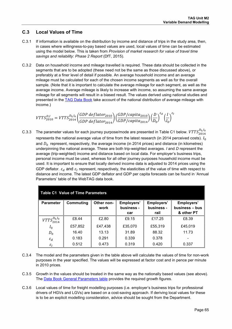
TAG Unit M2 Variable Demand Modelling
Page 65
C.3 Local Values of Time
C.3.1 If information is available on the distribution by income and distance of trips in the study area, then, in cases where willingness-to-pay based values are used, local values of time can be estimated using the model below. This is taken from Provision of market research for value of travel time savings and reliability: Phase 2 Report (DfT, 2015).
C.3.2 Data on household income and mileage travelled is required. These data should be collected in the segments that are to be adopted (these need not be the same as those discussed above), or preferably at a finer level of detail if possible. An average household income and an average mileage must be calculated for each of the chosen income segments as well as for the overall sample. (Note that it is important to calculate the average mileage for each segment, as well as the average income. Average mileage is likely to increase with income, so assuming the same average mileage for all segments will result in a biased result. The values derived using national studies and presented in the TAG Data Book take account of the national distribution of average mileage with income.)
C.3.3 The parameter values for each journey purpose/mode are presented in Table C1 below. 𝑉𝑉𝑉𝑉𝑉𝑉𝑉𝑉2014𝐷𝐷0,𝐼𝐼0
represents the national average value of time from the latest research (in 2014 perceived costs). 𝐼𝐼0 and 𝐷𝐷0 represent, respectively, the average income (in 2014 prices) and distance (in kilometres) underpinning the national average. These are both trip-weighted averages. I and D represent the average (trip-weighted) income and distance based on local data. For employer’s business trips, personal income must be used, whereas for all other journey purposes household income must be used. It is important to ensure that locally derived income data is adjusted to 2014 prices using the GDP deflator. 𝜀𝜀𝑑𝑑 and 𝜀𝜀𝐼𝐼 represent, respectively, the elasticities of the value of time with respect to distance and income. The latest GDP deflator and GDP per capita forecasts can be found in ‘Annual Parameters’ table of the WebTAG data book.
Table C1 Value of Time Parameters Parameter Commuting Other non-
work Employers’ business -
car
Employers’ business -
rail
Employers’ business – bus
& other PT
𝑉𝑉𝑉𝑉𝑉𝑉𝑉𝑉2014𝐷𝐷0,𝐼𝐼0 £8.44 £2.80 £9.15 £17.25 £8.39
𝐼𝐼0 £57,852 £47,438 £35,070 £55,319 £45,019 𝐷𝐷0 16.40 13.13 31.89 88.32 11.73 𝜀𝜀𝑑𝑑 0.183 0.291 0.339 0.378 - 𝜀𝜀𝐼𝐼 0.512 0.473 0.319 0.420 0.337
C.3.4 The model and the parameters given in the table above will calculate the values of time for non-work
purposes in the year specified. The values will be expressed at factor cost and in pence per minute in 2010 prices.
C.3.5 Growth in the values should be treated in the same way as the nationally based values (see above). The Data Book General Parameters table provides the required growth figures.
C.3.6 Local values of time for freight modelling purposes (i.e. employer’s business trips for professional drivers of HGVs and LGVs) are based on a cost-saving approach. If deriving local values for these is to be an explicit modelling consideration, advice should be sought from the Department.
𝑉𝑉𝑉𝑉𝑉𝑉𝑉𝑉2010𝐷𝐷,𝐼𝐼 = 𝑉𝑉𝑉𝑉𝑉𝑉𝑉𝑉2014
𝐷𝐷0,𝐼𝐼0 �𝐺𝐺𝐷𝐷𝐺𝐺 𝑑𝑑𝑑𝑑𝑑𝑑𝑑𝑑𝑑𝑑𝑑𝑑𝑑𝑑𝑑𝑑2010𝐺𝐺𝐷𝐷𝐺𝐺 𝑑𝑑𝑑𝑑𝑑𝑑𝑑𝑑𝑑𝑑𝑑𝑑𝑑𝑑𝑑𝑑2014
� �𝐺𝐺𝐷𝐷𝐺𝐺/𝑐𝑐𝑑𝑑𝑐𝑐𝑐𝑐𝑑𝑑𝑑𝑑2010𝐺𝐺𝐷𝐷𝐺𝐺/𝑐𝑐𝑑𝑑𝑐𝑐𝑐𝑐𝑑𝑑𝑑𝑑2014
� �𝐷𝐷𝐷𝐷0�𝜀𝜀𝑑𝑑�𝐼𝐼𝐼𝐼0�𝜀𝜀𝐼𝐼

TAG Unit M2 Variable Demand Modelling
Page 66
Appendix D Functional Forms for VDM
D.1 Detailed Advice on Functional Forms of VDM
D.1.1 Any model of the demand for travel relies on a mathematical mechanism which reflects how demand will change in response to a change in generalised cost. For example, the “own cost” elasticity mechanisms, described in Appendix A, modify an earlier estimate of demand using a curve which is as illustrated in Figure D.1: the demand approaches (and is asymptotic to) zero, but never actually falls to zero even at very high costs.
Figure D.1 “Own Cost” Elasticity Model Figure D.2 Choice Model
D.1.2 In a variable demand model, a different mechanism is normally used to apportion the total demand in a particular travel category between two or more available choices, as for example between car and public transport, or between many different destinations (see Figure D.2). In this case, when the generalised cost of the specified choice is very much lower than the alternative choices almost all travellers will choose it, and if it is very much greater then very few will. Again, the function used is asymptotic to 100% or zero, as illustrated in Figure D.2, since in any large population of travellers there will be a small but finite number who will take the apparently expensive choice. This arises even when only considering travellers with a car available and in general reflects how individual circumstances or choice preferences may be very different from the average.
D.1.3 The choice is unlikely to be based purely on simple formulations of generalised cost of travel: it will also depend upon appropriate zone or mode specific constants estimated in model calibration or implied by incremental models (see Section 4.3). They represent any reduction in disutility by making that choice (in other words, any gain of utility). For example, some modes will be inherently more attractive than others. Models assume that these hidden differences in the utility of travelling to any particular destination remain unchanged through time, and most therefore only need to reflect changes in the specific terms included in the generalised cost.
D.1.4 There are various mathematical functions that can provide a suitable relationship between travel demand and the disutility or generalised cost of a trip. These all offer broadly similar behaviour, but have subtly different mathematical properties. Appendix A discusses the equivalent subtle differences of power functions and exponential functions for own cost elasticity models, both of which can provide a convenient downward sloping relationship as shown in Figure D.1 and the parameters can be adjusted to give an elasticity of any required strength. For choice models a range of mathematical functions, most based on powers or exponentials, or both, can recreate the desired relationship. Ortuzar and Willumsen (2001) discusses the detailed functional forms of VDM models and the derivation of many of the forms in more detail.
Demand
Cost0
100%
Cheaper 0
Proportion choosing option 1
Difference in cost between option 1 and alternative(s)
More expensive

TAG Unit M2 Variable Demand Modelling
Page 67
Logit Formulation
D.1.5 Logit is a commonly used mathematical function to represent the behaviour shown in Figure D.2 because it is easy to manipulate mathematically. In general, it is formulated as:
( )( )∑ −
−=
pp U
UP
λλ
expexp
for an absolute model formulation
( )( )∑ ∆−
∆−=
pp U
UP
λλ
expexp
for an incremental model formulation
Where:
Pp is the proportion of travellers choosing alternative p out of q possibilities, Up is the disutility of option p (based on composite costs at lower levels in the hierarchy) and ∆Up is the change in disutility of option p. The summation in the denominator is over all q alternatives, including p. If there are only two choices this is called a binary logit model with the simple formulation P1=exp(-λU1) / [exp(-λU1) + exp(-λU2)]; for more choices it is referred to as a multinomial logit model.
D.1.6 The mechanism should be applied separately to different segments of travel, such as trip purposes, as the sensitivity of the model is likely to be different in each category. For different trip purposes, for example, the logit sensitivity parameter (lambda) is likely to be numerically larger where there is more freedom to choose. Thus more optional travel, such as shopping trips, tends to be more elastic and have a numerically larger lambda value than, say, travel to work.
D.1.7 The multinomial logit choice function is one of a number of possible formulations of “random utility” models in which a random component is added to the deterministic disutility21 of choice p as follows:
∑ += pnnnp xU εβ
Where the disutility Up of choice p is calculated as the sum of:
• the generalised cost Gp = ∑n βn xn of choice p, with the set of cost components xn weighted by coefficients βn, summed over all components relevant to choice p as explained in Section 3.1. (For example, if G is measured in units of time, x might be the money cost of a journey and β the inverse of Value of Time), and
• a random component εp used to represent variations in the situation or tastes of individual travellers, or modelling errors, or unobserved elements of the alternative choices. (In the most general case this random component can depend on both the traveller and on the choice alternative).
D.1.8 A choice-specific calibration constant (i.e. constant specific to the mode or areas used in calibration) could be added to the generalised cost function to adjust the calculated choice to the observed value.
D.1.9 A random utility model assumes that the alternative with the minimum disutility is chosen, so that a probabilistic model results.
D.1.10 The assumed statistical distribution of the error terms or residuals εp determines the exact mathematical formulation. For example, assuming one particular distribution for the random components, that they are Independent and Identically Distributed (IID) extreme value variables, leads to the widely-used multinomial logit model:
21 For transport modelling the utility is generally the negative of the value of generalised cost (or disutility).

TAG Unit M2 Variable Demand Modelling
Page 68
∑ −−
=)exp()exp(
ptotp U
UTT
λλ
Where λ is the positive sensitivity parameter and Up is the disutility / generalised cost.
D.1.11 The elasticity of demand in this formulation is -λUp(1-Tp/Ttot), so that the elasticity scales with U, and tends to be larger for longer trips for a given value of λ and larger for choices with a small share of the total. If those implications are inappropriate for the model area a different functional form or a series of calibration areas should be used to produce a model with suitable implications.
D.1.12 Other forms such as the power function or the Tanner function, which have been described in relation to ‘own cost’ elasticity models, or formulations assuming a normal distribution of error terms (Probit models) are possible but little used in modelling for scheme appraisal. However, different formulations of the logit model which have less restrictive statistical assumptions are also possible.
D.2 Trip Frequency
D.2.1 The elasticity function could be a power function or an exponential function. However, if logit is used for the other mechanisms, a similar exponential function is generally used to adjust trip frequency. In this case, the function operates simply as an elasticity with respect to disutility or generalised cost, since the relevant choice is to travel or not to travel, and the disutility of not travelling remains constant:
)exp()exp(
0
0
icompfreq
icompfreqii G
GTT
⋅−−
=λλ
D.2.2 Where Ti is the number of trips from origin zone i, prefix 0 denotes the base values, λfreq is the choice sensitivity parameter for the trip frequency stage and the generalised cost Gicomp is the composite cost or disutility calculated across the trip origins. The compound cost of travel for trips from a given zone must be calculated across all available choices lower in the hierarchy (i.e. destination, mode and time period choices where available). See Section 3.2 for details.
D.3 Mode Choice
D.3.1 For mode choice, trips between each origin-destination pair of zones are allocated to the available modes according to the composite disutility or generalised cost of travel by that mode:
∑ −−
=)exp(
)exp(
ijmmodem
ijnmodeijijn G
GTT
λλ
if mode choice is the only demand response; and
∑ −−
=)exp(
)exp(
ijmcompmodem
ijncompmodeijijn G
GTT
λλ
if mode choice is a more sensitive response than distribution. Tijn is the number of trips choosing mode n from a set of modes m and λmode is the choice sensitivity parameter for the trip mode stage. The composite cost Gijncomp is calculated across the time periods in a way that weights the average according to the probability of choosing that period. The summation is across all available modes m, including n. However, if mode choice is less sensitive than distribution, the composite cost Gimcomp must be calculated to forecast an overall modal split for each origin zone. If there is more than one public transport mode it is usual to use a nested or hierarchical model, with a higher level split between car and public transport (and possibly active modes also). The allocation to the different

TAG Unit M2 Variable Demand Modelling
Page 69
public transport modes (and between walk and cycle if modelled) is then made at a lower level (see Section 4.5) or possibly in assignment.
D.4 Time of day choice
D.4.1 Macro time period choice (or the allocation of trips between broad time periods) assuming this is the most sensitive response takes the form:
∑ −−
=)exp()exp(
ijmttimet
ijmstimeijmijms G
GTT
λλ
Where Tijms is the number of trips between zones i and j by mode m in time period s. Gijmt is the disutility or generalised cost of travel between zones i and j by mode m in time period t, which may typically be peak and inter-peak and λtime is the choice sensitivity parameter for the time period stage. However, if it is above mode choice and distribution, it would take the form:
∑ −−
=)exp(
)exp(
ittimet
istimeiis G
GTTλλ
Where Tis is the number of trips in Zone i in time period s and Gis is the disutility or generalised cost of travel in zone i in time period s.
D.5 Trip Distribution
D.5.1 The general form for a doubly-constrained distribution model is:
)( ijjijiij GfDObaT =
Where:
Tij is the number of trips from zone i to zone j,
Oi is the total number of trips originating in zone i
Dj is the total number of trips ending in zone j
Tij depends on the travel disutility or cost via the deterrence function as f(Gij),
Which in most models is a logit function
∑ −−
)exp()exp(
ikcompk
ijcompdist
istGdG
λλ
Where:
Gijcomp is a composite cost calculated across the available modes and time periods, if these choices are to be calculated after distribution
ai and bj are balancing factors which are only used when the model is singly or doubly constrained to ensure that ∑j Tij = Oi (ie there are Oi trips originating in zone i), and ∑i Tij = Dj (ie there are Dj trips ending in zone j), and are calculated at each iteration of the constraining routine as ai = 1/∑j bj Dj
f(Gij) or bj = 1/∑i aI OI f(Gij)
D.5.2 In the above equation, Tij is proportional to Oi, the total number of trips originating in zone i,Tij is also proportional to Dj, the total number of trips ending in zone j, or alternatively in a singly-constrained model the facilities available in zone j (numbers of jobs, retail floorspace, etc) so that the number of trips ending in j depends also on the competing attractivities of other zones.
D.5.3 If the distribution model is singly (origin)-constrained the equivalent destination choice model is:

TAG Unit M2 Variable Demand Modelling
Page 70
∑=
kikk
ijjiij GfD
GfDOT
)()(
which satisfies the origin constraint:
ij
ij OT =∑
If the distribution model is doubly-constrained, the destination choice model is:
∑=
kikkk
ijjjiij GfDb
GfDbOT
)()(
where the bj‘s are calculated iteratively to satisfy the destination constraint:
ji
ij DT =∑
In the case of origin constrained trip distribution Dj is some function of the attractiveness of destination zone j, and in the case of a doubly-constrained trip distribution model Oi and Dj represent total origin and total destination trip ends respectively. Gij represents the generalised costs of travel between i and j and f(Gij) the deterrence function which may or may not contain (multiplicative or additive) Kij factors.
D.5.4 In the above equation there are a number of different deterrence function forms that can be adopted for f(Gij). In a true gravity model the deterrence functions are power functions f(Gij) = Gija (and originally zone pair distance was used instead of G), but it is standard now to use an exponential form:
)exp()( ijdistij GGf λ−=
or with multiplicative Kij factors:
)exp()( ijdistijij GKGf λ−=
or with additive Kij factors:
)(exp()( ijijdistij KGGf +−= λ )
D.5.5 The calculation of costs should use composite cost Gijcomp (see Section 4.5) calculated only across the stages lower in the hierarchy of mechanisms.

TAG Unit M2 Variable Demand Modelling
Page 71
Appendix E Incremental Model Formulation E.1.1 When specifying an incremental hierarchical logit model, scaling parameters as provided in section
5.6 could be used. These parameters (thetas) refer to the probability of nests of alternatives or composite alternatives. They reflect the ratios of the lambdas for different response mechanisms as one moves up the model structure. The scaling parameters are applied to the logsums of the composite or nested alternatives. They should have a value between 0 and 1 if the responses have been included in the correct order in the model, such that the sensitivity of the responses changes down the hierarchy from lower to higher.
E.1.2 The standard incremental multinomial logit model is given as
( )( )∑ ∆∆
=
qqq
ppp Up
Upp
θθ
expexp0
0
where
pp is the forecast probability of choosing alternative p
0pp is the reference case probability of choosing alternative p (calculated from the input
reference demand)
θ is the scaling parameter (always =1 for the bottom level of the hierarchy)
pU∆ is the change in the utility of alternative p
For the choice at the bottom level of the hierarchy the change in utility is given by
( )0pipp CCU −−=∆ λ
Where
0pC is the reference generalised cost and
pC is the forecast generalised cost, skimmed from the latest assignment
λ is the spread or dispersion parameter (defined by the user); it should be positive
For choices above the bottom level of the hierarchy the change in utility is the composite change over the alternatives in the level below:
( )∑ ∆=∆p
pp UpU expln 0*
This model formulation can be used for mode choice, time period choice and singly constrained distribution
E.1.3 A modified version of the logit model is used for doubly-constrained distribution as follows:
( )( )∑
=
∆
∆= N
kikikk
ijijjiij
UTB
UTBOT
1
0
0
exp
exp
θ
θ
Where
ijT is the forecast number of trips travelling from zone i to zone j

TAG Unit M2 Variable Demand Modelling
Page 72
0ijT is the reference case number of trips travelling from zone i to zone j
iO is the number of trips travelling from zone i
jB are destination-based constants, normalised so that ∑j
jB is equal to the number of zones
Note that destination constraints are summed over all person types within a purpose, and across all modes and time periods, if those choices have been modelled.
The change in composite utility for origin zone a is calculated using:
( )∑ ∆=∆b
aba
abba U
OTBU θexpln 0
0*
The illustrative parameter values currently provided in Section 5.6 can be used in an incremental model structure as follows:
Suppose we assume the follow choices available
• Single trip purpose (say commuting) split into:
• Two person types (say car available and car not available)
• Mode choice – between car and public transport (all sub modes), no active modes
• Car available hierarchy (from top to bottom): frequency, mode choice, macro time period choice, distribution (doubly constrained)
• Car not available hierarchy (from top to bottom): frequency, time period choice, distribution (doubly constrained)
E.2 Inputs
E.2.1 Inputs to the demand model are:
0ijmtpcC reference generalised cost from zone i to zone j by mode m in time period t, trip purpose p,
person type c
ijmtpcC corresponding forecast generalised cost, skimmed from latest assignment
0ijmtpcT corresponding reference demand, defined via the user interface
In all the above, there is no data for the highway mode for the no-car person type
E.3 Bottom level utilities
E.3.1 The first step is to calculate the change in utility for the lowest level of the hierarchy:
( )0, ijmtpcijmtpcmcdistijmtpc CCU −−=∆ λ
Where mcdist ,λ is the mode m-and person type c specific distribution λ parameter
E.4 Doubly-constrained distribution
E.4.1 Since the lowest level is a doubly constrained distribution model there is a need to find the balancing factors jpB . This requires solving the set of equations given by:

TAG Unit M2 Variable Demand Modelling
Page 73
( )( )∑
=
∆
∆= N
kikmtpcikmtpckp
ijmtpcijmtpcjpimtpcijmtpc
UTB
UTBOT
1
0
0
exp
exp
such that the destination trip end constraints are met:
jpimtc
ijmtpc DT =∑
The destination constraints are calculated from the reference demand matrix:
∑=imtc
ijmtpcjp TD 0
Note that the destination trip end constraints depend on destination and trip purpose only.
The balancing factors are normalised so that
NBj
jp =∑
where N is the number of destination zones.
On the first iteration only of the demand model, the origin trip ends are calculated from the reference demand matrix:
∑=j
ijmtpcimtpc TO 0
For subsequent iterations they are obtained from the application of the conditional probabilities described below.
E.5 Composite Utilities
E.5.1 The change in the composite utility from the distribution, time period choice and mode choice stages is then calculated:
( )∑ ∆=∆j
ijmtpcimtpc
ijmtpcjpimtpc U
OT
BU expln 0
0*
( )∑ ∆=∆t
imtpctimecimcptimpc UpU *0
|* expln θ
( )∑ ∆=∆m
impcmodecicpmipc UpU *0
|* expln θ
(car available person type) **impcipc UU ∆=∆ (car not available person type, m= PT)
The reference case probabilities are calculated from the input reference demand as follows:
∑∑
=
jtkijktpc
jtijmtpc
icpm T
Tp 0
0
0|
∑∑
=
kijmkpc
jijmtpc
imcpt T
Tp 0
0
0|
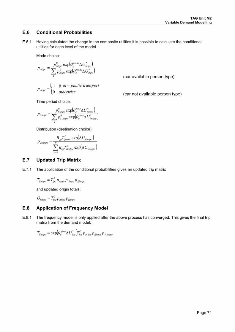
TAG Unit M2 Variable Demand Modelling
Page 74
E.6 Conditional Probabilities
E.6.1 Having calculated the change in the composite utilities it is possible to calculate the conditional utilities for each level of the model
Mode choice:
( )( )∑ ∆
∆=
kikpc
modecipck
impcmodecipcm
ipcm UpUp
p *0|
*0|
| expexp
θθ
(car available person type)
=
=otherwise
transportpublicmifp ipcm 0
1|
(car not available person type)
Time period choice:
( )( )∑ ∆
∆=
kimkpc
timecimpck
imtpctimecimpct
impct UpUp
p *0|
*0|
| expexp
θθ
Distribution (destination choice):
( )( )∑
=
∆
∆= N
kikmtpcikmtpckp
ijmtpcijmtpcjpimtpcj
UTB
UTBp
1
0
0
|
exp
exp
E.7 Updated Trip Matrix
E.7.1 The application of the conditional probabilities gives an updated trip matrix
imtpcjimpctipcmipcijmtpc pppTT |||0=
and updated origin totals:
impctipcmipcimtpc ppTO ||0=
E.8 Application of Frequency Model
E.8.1 The frequency model is only applied after the above process has converged. This gives the final trip matrix from the demand model:
( ) imtpcjimpctipcmipcipcfreq
cijmtpc pppTUT |||0*exp ∆= θ

TAG Unit M2 Variable Demand Modelling
Page 75
Appendix F Absolute Model Formulation F.1.1 The illustrative parameter values currently provided in Section 5.6 can be used in an absolute model
structure as follows:
F.2 Assumed Nesting
Layer 1 (Highest): Frequency
Layer 2: Main Mode
Layer 3: Macro Time Period
Layer 4 (Lowest): Destination
F.3 Notation
Trip origin i Trip destination j, k
Macro time period t, s Main mode m, r
Trips T Generalised cost G
Distribution parameter λdist Attraction factor B
Composite utility U Tree parameters θtime, θmode, θfreq
Pivot (reference) trips 0T Pivot (reference) utilities 0U
F.4 Composite Utilities:
F.4.1 The incremental composite utilities summed over the choices in the destination layer are given by:
∑ ∑−−=j j
jijmtdistjimt BGBU ln)exp(ln λ
F.4.2 Initial values for the attraction factors Bj are needed (see notes given later about the destination choice probabilities).
F.4.3 The composite utilities summed over choices in the time period layer are given by
∑=t
imttimeim UU )exp(ln θ
This uses the scaling parameter θtime which reflects the ratio of the lambda for macro time period to the lambda for distribution.
F.4.4 The incremental composite utilities summed over the main mode layer are given by
∑=m
immodei UU )exp(ln θ
These composite utilities are used to calculate the choice probabilities in the various layers as follows. Where required, base utilities can also be calculated from the same composite utility formulae given above, but using base values for the generalised costs and balancing factors.
F.5 Choice Probabilities:
F.5.1 Layer 1, Frequency:

TAG Unit M2 Variable Demand Modelling
Page 76
)exp()exp(
0
0
ifreq
ifreqii U
UTT
θθ
=
Note that this calculation makes use of a reference utility value
F.5.2 Layer 2, Main Mode Choice (m):
∑=
rirmode
immodeiim U
UTT)exp()exp(
θθ
F.5.3 Layer 3, Macro Time Period Choice (t):
∑=
simstime
imttimeimimt U
UTT)exp()exp(
θθ
F.5.4 Layer 4, Destination Choice (j):
∑ −
−=
kikmtdistk
ijmtdistjimtijmt GB
GBTT
)exp()exp(
λλ
Notes
F.5.5 All distribution models satisfy the constraint: ∑ =j
imtijmt TT
F.5.6 For doubly constrained destination choice models Bj needs to be calculated to satisfy the additional constraint: ∑ =
imtjijmt TT
F.5.7 Some models employ area specific, mode specific, and time period specific constants and/or sensitivity parameters which vary by zone or zone pairs. Advice on these matters can be found in Appendix D.

TAG Unit M2 Variable Demand Modelling
Page 77
Appendix G Estimation of Transferred Mode Choice Models Importing Mode Choice Model Parameters
G.1.1 The foundation of a mode choice model using imported model parameters is the utility formulation describing the choice alternatives, i.e.:
∑=k
nikkni xV β
where niV is the deterministic component of utility derived from alternative i by user n, nikx are the
relevant attribute values (k) relating to alternative i for user n and kβ are the model parameters indicating the relative importance of each attribute.
G.1.2 The specific attribute values, for each choice observation, will usually be derived from networks or other databases, e.g. fares. In bespoke models, the βs will be estimated such that the observed choices are best represented. For transferred models, these parameters are inputs to the modelling. Specific local calibration will require data from either Stated Preference (SP) or Revealed Preference (RP) studies. Where these are impractical or unnecessary, several national indicative sources may be used:
• Values in the TAG Data Book;
• TRL Report TRL593, The demand for public transport: a practical guide, for information on the relative valuations of public transport journey components;
• Passenger Demand Forecasting Handbook (PDFH), in cases where access to this source is possible;
• a mixture of the above (including some SP or RP where available).
G.1.3 It is essential that the βs are measured in consistent units. Two units of measure are generally used: Generalised Costs (GC) and Generalised Times (GT).
G.1.4 In the generalised cost formulation, all in-vehicle and out-of-vehicle time components (x) are multiplied by appropriate values, by purpose and journey component (β), to convert them into monetary values. For example, if a typical generalised cost formulation for a rail journey were to be considered, it may include in-vehicle time, out-of-vehicle time and other components, for example:
farexfersxfers
xtimeVOTxtimewaittimeeVOTwaittimacctimeVOTacctimerailtimeeVOTrailtimRailGC
xxxxxxV
+++++=
βββββ
where
eVOTrailtimβ value of time for travel by rail, for specific purpose of travel
VOTacctimeβ value of time for access and egress to rail
eVOTwaittimβ value of time for (first) wait time
VOTxtimeβ value of time for interchange time
xfersβ monetary penalty value of an interchange

TAG Unit M2 Variable Demand Modelling
Page 78
G.1.5 When using generalised times, all in-vehicle and out-of-vehicle time components (x) must be multiplied by appropriate values, by purpose and journey component (β), to convert the component into units of time. The same example rail journey specified above would now be specified as follows:
fareVOTxfersxfersxtimextimewaittimewaittimeacctimeacctimerailtimeRailGT xxxxxxV /1βββββ +++++=
where
acctimeβ value of access and egress time, relative to rail in-vehicle time
waittimeβ value of (first) wait time, relative to rail in-vehicle time
xtimeβ value of interchange time, relative to rail in-vehicle time
xfersβ time penalty value (in terms of rail in-vehicle time) of an interchange
VOT/1β value of money, in terms of rail time (1 / VOT)
G.1.6 TAG Data Book has assumptions that should be made for changes in value of time into the future, and though these recommendations relate strictly to their use in appraisal, they may be taken as representing reasonable practice for modelling as well.
G.1.7 It is not recommended to change the model alternative-specific constants (ASCs) as a result of forecast changes in income and/or values of time, on the basis that the unmeasured component of utility, as measured by the alternative-specific constants, has no expected relationship with income.
G.1.8 For models using imported parameters, it is recommended to use local RP data to calibrate both the model scale and ASCs.
Recalibration of Transferred Mode Choice Models
G.1.9 The advantage of using disaggregate or semi-aggregate RP data for recalibration of transferred models is that these data allow the direct estimation of the model scale and ASCs through Maximum Likelihood estimation of a logit model, with the accompanying tests of coefficient accuracy and significance that can be undertaken (see Supplementary Guidance on Bespoke Mode Choice Models) and model fit. Specifically, the model results will indicate the accuracy of the scale coefficient and provide evidence of its validity, i.e. whether it is significantly different from zero. The methodology for identification of the model scale and alternative specific constants is set out below.
G.1.10 First, for each observation, the generalised cost or time term is calculated, e.g. VRail , VBus and VCar below. The utility equation for each alternative is then defined by the generalised cost or time term, multiplied by a scale (βscale) and a constant (added to all but one alternative).
RailconstRailscaleRailAdj VV ββ +=
BusconstBusscaleBusAdj VV ββ +=
CarscaleCarAdj VV β=
G.1.11 The scale parameter and ASCs are then estimated directly using standard software for estimating logit models. In the specification of the utilities it does not matter whether the ASCs are multiplied by the scale or not, because in a logit model it is the differences between utility equations for different alternatives which are important. It is important, however, that the definition of the constants in the forecasting model is consistent with that used for model estimation, i.e. scaled or unscaled.

TAG Unit M2 Variable Demand Modelling
Page 79
G.1.12 If disaggregate RP data are used for the model calibration, then there is further scope for identifying socio-economic terms, reflecting for example preferences for specific modes. These terms would be included directly in the utility equation; for example if a term for high-income travellers was to be tested for rail, the following term would be included in the rail utility as follows:
)( highincomeVV HighIncomeRailconstRailscaleRailAdj =++= βββ
G.1.13 Nested model structures can also be tested using the scaled utilities. Separate scales, constants and model structures should be calculated for each travel purpose. It is important that the scaled model is used for any scenario tests.
G.1.14 In the simplest case, aggregate information on mode shares may be used to recalibrate ASCs and information on mode shares by trip length could be used to calibrate the model scale. It is emphasised that semi-aggregate and disaggregate data provide much better information for calibration of the model scale and therefore the use of aggregate information is only recommended for the recalibration of models for small schemes.
G.1.15 Adjustments to the ASCs can be made iteratively, by running the mode choice model using the generalised cost or time equations for utility and by then examining how closely the mode shares are replicated. Adjustments equal to ln(observed share/predicted share) are added to the utility for each mode, until the predicted shares closely reproduce the observed shares.
G.1.16 Adjustments to the scale also have to be made iteratively, by running the model and examining how closely the mode shares by trip length category are replicated. Adjustments to the model scale must be made until the mode shares are approximately correct.
G.1.17 It is noted that the scale and constants are inter-related and any amendment to the scale will impact the mode shares and vice versa.
G.1.18 An alternative validation procedure to obtain a model scale is to adjust the scale until known or desired elasticities are reproduced. Again, adjustments to the constants will also be required to reproduce the observed overall mode shares.
G.1.19 Separate scales and constants should be calculated for each travel purpose.
Transfer of Model Systems
G.1.20 In this case, an entire model system is available which applies to one area and is to be transferred to the area in which a proposed scheme is to be appraised.
G.1.21 The transfer can be approached either component by component or for the system as a whole. In any case, models for separate travel purposes should be transferred separately.
G.1.22 When separate components of a model system are transferred, the procedure is that the transferred model is used to specify the utility functions of the alternatives in each component (destination choice, mode choice etc.) and that ASCs and scale factors are then estimated to calibrate the model to local conditions.
G.1.23 This procedure closely follows that described in the previous section, except that an existing model is used to define the utility functions, rather than the analyst defining the functions and then looking to find suitable coefficients for the variables he or she thought should be included.
G.1.24 Data, for example from networks, are required to describe the explanatory variables in the model utility equations for the area of interest.
G.1.25 In the transfer of a disaggregate mode choice model, or disaggregate model system, scale parameters are estimated for a limited number of functional subgroups of explanatory variables such as level-of-service attributes, personal characteristics, other local effects, etc.. The idea is that each

TAG Unit M2 Variable Demand Modelling
Page 80
subgroup has a similar functionality, and different groupings may be tested as part of the estimation procedure.
G.1.26 Because the scales of the component models are changed by this process, care must be taken to maintain the validity of the model structure. That is, if the mode choice model is more sensitive than the destination choice model, so that an appropriate hierarchical structure is used in the original model, then the scales applied to calibrate these models to the new situation must be checked to ensure that the relative sensitivities remain consistent with the hierarchy in the model. If this is not the case, then the model may need to be restructured.
G.1.27 An alternative approach is to transfer the entire model system and to preserve the structural coefficients that are used in that model. Essentially this means that a single scale is applied to the entire model. The advantages of this approach are that less data is required in the fully modelled area and that the structural problems mentioned above cannot arise. The disadvantage is that a model transferred in this way will fit the local circumstances less well. In any case, ASCs should be calibrated to match the overall mode shares in the new area.
Transferred Mode Choice Model Validation
G.1.28 It should be verified that the relative value of the model coefficients, e.g. implied values of time, will be reasonable for transferred models, which are an input to the modelling process.
G.1.29 In the cases where the model scale and constants are estimated directly as part of the model transfer recalibration procedure, the model results will indicate the accuracy of the scale coefficient and can provide evidence of its validity, i.e. whether it is significantly different from zero.
G.1.30 The presence of disaggregate RP data allows examination of model predictions and observed choices to be examined across socio-economic and possibly geographical sub-segments.

TAG Unit M2 Variable Demand Modelling
Page 81
Appendix H Use of DIADEM
H.1 Introduction
H.1.1 The DIADEM procedures provide an adjustable hierarchical structure of trip frequency, mode choice, distribution, and time of day choice (macro and micro), and an interface to assignment. It is also possible to use DIADEM for a simple “own-cost” elasticity calculation where applicable. The DIADEM framework controls iteration within assignment, and between demand and assignment, to ensure that the calculation reaches an acceptable equilibrium.
H.1.2 At present, DIADEM has been developed with an interface to the CONTRAM and SATURN assignment packages. It is expected, however, that the suppliers of other assignment packages will provide equivalent functionality or suitable interfaces with DIADEM; so that it can be used with whatever assignment model is available for the scheme to be assessed. As ever, there is no monopoly on the most convenient way to achieve best practice: as with choice of assignment package; which one to adopt is a matter of individual preferences and priorities. If a decision is made to use DIADEM then Section H.2 provides a summary of the approach. If other software is to be used then Section 6.2 gives guidance on how alternative software should be used.
H.2 DIADEM Procedures
H.2.1 The DIADEM procedures cover all the demand-side issues that must be considered when applying multi-stage models and provides the user with the necessary choice between alternative formulations and full control over each aspect.
Model Type
H.2.2 Demand responses: DIADEM allows the following responses to be included:
• the elasticity model has a 2-parameter Tanner form, which is intended to be used in its extremes, setting one of the parameters to 0 to return either a power or an exponential form, as discussed in Section 4. The use of both parameters together in the Tanner form is not recommended.
• the trip frequency model is an exponential elasticity function, but unlike general elasticity models (which operate at the OD level), the trip frequency model applies to the zone level, using composite zone (accessibility) costs as discussed in Section 4.
• the mode choice model is a binomial logit formulation. The model does not automate the hierarchical modelling of public transport modes i.e. sub mode choice. Any lower-level split between different public transport modes would have to be estimated independently or at assignment as discussed in Section 4. However, this sub-mode choice will rarely be needed in a road-based scheme appraisal.
• the trip distribution model can be singly-origin constrained or singly-destination constrained (to approximate to Production /Attraction constraints) or doubly-constrained as discussed in Section 4.
• a macro time period choice model in logit form is currently available.
• a micro time period choice model using HADES is also available.
H.2.3 For a discussion on alternative model forms of departure-time choice, see Batley et al (2001).
Model hierarchy
H.2.4 DIADEM allows a different range of responses, a different model form and a different hierarchy to be applied to each individual purpose and traveller type combination.

TAG Unit M2 Variable Demand Modelling
Page 82
Model parameters
H.2.5 Each modelled response is driven by a single user-defined lambda parameter, per purpose and traveller type combination, apart from the elasticity models which as Tanner formulations are driven by two parameters (though normally one of these should be set to zero, returning the Tanner function to either a power or an exponential function).
Generalised costs
H.2.6 Generalised cost coefficients are defined for each purpose and traveller type combination, allowing for time, distance and monetary components. Any weighting of in-vehicle, waiting or walking time must be done within the assignment stage or outside the DIADEM environment, and a similar argument applies to crowding effects. The analyst is provided with a flexible tool in DIADEM to arrange the sequence of demand responses and warned if the proposed sequence does not reflect demand sensitivities. However, the analyst will still need to ensure that the definitions of generalised cost in the demand and assignment phases include all the necessary terms and are sufficiently compatible.
Model running
H.2.7 Guidance on how to run the DIADEM software is given in the user guide to the software. It should be noted that the solution closest to equilibrium may not necessarily be the one produced by the last iteration of the DIADEM demand/assignment modelling system. The solution from the iteration with the lowest GAP value should be used for appraisal purposes. This may require an additional run of the assignment package using this ‘best’ trip matrix to obtain a converged solution.