Table of Contents - University of Michiganriboch/publications/NACADuct.pdf · Table of Contents...

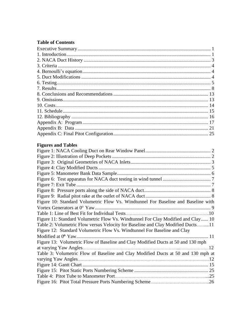
Table of Contents

Executive Summary ............................................................................................................ 1

1. Introduction ..................................................................................................................... 1 2. NACA Duct History ....................................................................................................... 3 3. Criteria ............................................................................................................................ 4 4. Bernoulli’s equation ........................................................................................................ 4 5. Duct Modifications ......................................................................................................... 4

6. Testing............................................................................................................................. 5 7. Results ............................................................................................................................. 8 8. Conclusions and Recommendations ............................................................................. 13 9. Omissions ...................................................................................................................... 13 10. Costs ............................................................................................................................ 14

11. Schedule ...................................................................................................................... 15

12. Bibliography ............................................................................................................... 16 Appendix A: Program ...................................................................................................... 17

Appendix B: Data ............................................................................................................ 21 Appendix C: Final Pitot Configuration ............................................................................. 25

Figures and Tables Figure 1: NACA Cooling Duct on Rear Window Panel ..................................................... 2

Figure 2: Illustration of Deep Pockets ................................................................................ 2 Figure 3: Original Geometries of NACA Inlets ................................................................. 3 Figure 4: Clay Modified Ducts ........................................................................................... 5

Figure 5: Manometer Bank Data Sample............................................................................ 6

Figure 6: Test apparatus for NACA duct testing in wind tunnel ....................................... 7

Figure 7: Exit Tube ............................................................................................................. 7 Figure 8: Pressure ports along the side of NACA duct ...................................................... 8

Figure 9: Radial pitot rake at the outlet of NACA duct ..................................................... 8 Figure 10: Standard Volumetric Flow Vs. Windtunnel For Baseline and Baseline with

Vortex Generators at 0 Yaw .............................................................................................. 9

Table 1: Line of Best Fit for Individual Tests…………………………………………………….10

Figure 11: Standard Volumetric Flow Vs. Windtunnel For Clay Modified and Clay ...... 10

Table 2: Volumetric Flow versus Velocity for Baseline and Clay Modified Ducts……....11 Figure 12: Standard Volumetric Flow Vs. Windtunnel For Baseline and Clay

Modified at 0 Yaw ........................................................................................................... 11

Figure 13: Volumetric Flow of Baseline and Clay Modified Ducts at 50 and 130 mph

at varying Yaw Angles……………………………………………………………...…………………12

Table 3: Volumetric Flow of Baseline and Clay Modified Ducts at 50 and 130 mph at

varying Yaw Angles……………………………………………………………………………………12

Figure 14: Gantt Chart ...................................................................................................... 15 Figure 15: Pitot Static Ports Numbering Scheme ............................................................ 25 Table 4: Pitot Tube to Manometer Port…………………………………………………………....25

Figure 16: Pitot Total Pressure Ports Numbering Scheme…………………………………….26

1

Executive Summary

For the past 4 months Team RentDR has been studying cooling ducts for Dodge Racing

trying to find ways to increase the mass flow. We were working on NACA (National

Advisory Committee for Aeronautics) ducts that are used in NASCAR to help cool the

inside of the racecars. As this is a continuation of previous work our goal was to expand

on what had been already done. After we studied what had been done we decided on

what we thought would be best to proceed forward with. Since the previous work only

tested a NACA duct with clay modification and vortex generators we decided our

primary goal would be to see which had a more significant effect on the increase of mass

flow. We used the University of Michigan’s 5 ft x 7 ft wind tunnel to best simulate

actual racing conditions. We were able to vary the speed from 20 miles per hour (mph)

all the way to 160 mph. While NASCAR racecars can reach speeds averaging 180 mph

on the superspeedways we felt that 160 mph would be significant since most of the

racetracks that NASCAR uses do not reach such high speeds.

Using a testing apparatus that was constructed previously, we were able to connect

multiple static and total pressure ports to a manometer bank and tested three different

variations that had been made to the ducts. After analyzing our data we found that only

clay modifications gave an improvement of 37.3% increased mass air flow at 130 mph

into the ducts. Based on this and due to the fact that we found that the vortex generators

we were using hindered the flow, we recommend that Dodge Racing manufacture and

implement these new duct designs into their racecars. We feel that this modification

would be a very cheap and simple solution to implement.

1. Introduction

In the world of NASCAR every advantage a team can get over another team is very

important. Many teams resort to cheating to get that advantage. This can be seen every

year when there is a story in the news about how a team was caught for cheating. There

is even a motto used in NASCAR that states “If you ain’t cheatin’ you ain’t tryin’!”. This

shows how much teams are trying to get ahead of everyone else to improve their racecars.

Dodge Racing is going about improving their cars the legal way by tasking us, Team

RentDR in finding a way to improve the mass flow into the cooling ducts that are placed

on the sides of the racecar.

2

Figure 1: NACA Cooling Duct on Rear Window Panel

Our work was a continuation of previous work done by the AERO 405 group working on

this problem last semester. The main thing we were able to achieve was the ability to test

the ducts in the 5 ft x 7 ft wind tunnel. Previously the ducts were only tested in the 2 ft x

2 ft wind tunnel and the boundary layers were studied. In studying the boundary layer

the previous group thought of adding vortex generators to help keep the flow attached. In

addition, they added clay to try and smooth the flow into the duct. The way the ducts are

currently designed is there are deep side pockets on either side of where the flow enters

the circular tube of the duct, as is shown below in Figure 2. The previous team thought

by eliminating these pockets that the flow would not need to be turned and would go

directly into the tubing.

Figure 2: Illustration of Deep Pockets

3

Since we were trying to improve mass flow we wanted to test how the clay and vortex

generators affected the mass flow separately since this was not done before. Another

scenario that we wanted to investigate was the yaw angle of the duct since this also was

not tested previously. The ultimate purpose of the duct is to cool, so the more air

entering the ducts the more effective the cooling will be. By investigating the design of

the duct and how it is aligned with the flow we hope to present an improved model that

can be used in the future.

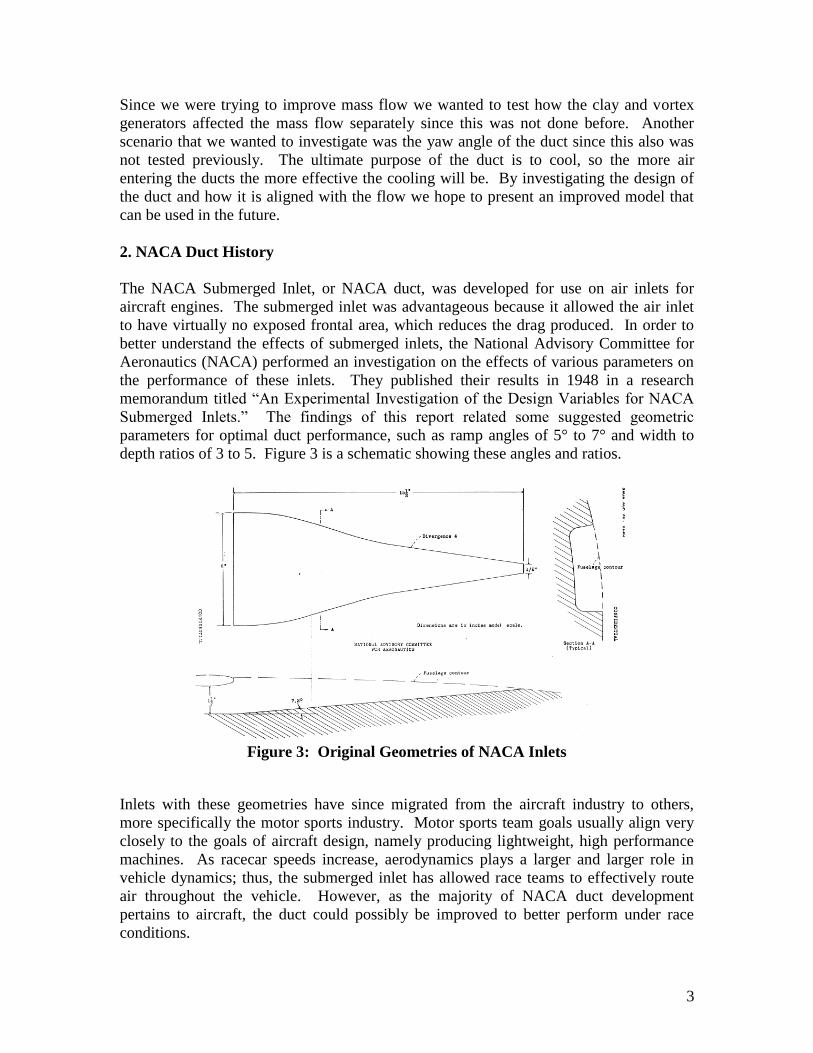
2. NACA Duct History

The NACA Submerged Inlet, or NACA duct, was developed for use on air inlets for

aircraft engines. The submerged inlet was advantageous because it allowed the air inlet

to have virtually no exposed frontal area, which reduces the drag produced. In order to

better understand the effects of submerged inlets, the National Advisory Committee for

Aeronautics (NACA) performed an investigation on the effects of various parameters on

the performance of these inlets. They published their results in 1948 in a research

memorandum titled “An Experimental Investigation of the Design Variables for NACA

Submerged Inlets.” The findings of this report related some suggested geometric

parameters for optimal duct performance, such as ramp angles of 5° to 7° and width to

depth ratios of 3 to 5. Figure 3 is a schematic showing these angles and ratios.

Figure 3: Original Geometries of NACA Inlets

Inlets with these geometries have since migrated from the aircraft industry to others,

more specifically the motor sports industry. Motor sports team goals usually align very

closely to the goals of aircraft design, namely producing lightweight, high performance

machines. As racecar speeds increase, aerodynamics plays a larger and larger role in

vehicle dynamics; thus, the submerged inlet has allowed race teams to effectively route

air throughout the vehicle. However, as the majority of NACA duct development

pertains to aircraft, the duct could possibly be improved to better perform under race

conditions.

4

3. Criteria

The main focus for this examination was increasing the mass flow through the specified

3-inch inlet hose. As this inlet size is standard for this application, different duct

geometries are the most effective way of changing the airflow through the duct.

Therefore, this study concentrates almost entirely on measuring the mass flow through

the duct. The four ducts tested were evaluated solely on the mass airflow through the

hose. While the drag produced by the different ducts is very important, our test apparatus

was not sufficient to ensure accurate data. The drag produced by the ducts can be studied

at a later date at a facility with a larger wind tunnel to allow full scale testing of the entire

racecar.

4. Bernoulli’s equation

The governing equation that was used to determine velocity through the outlet of the duct

was Bernoulli’s equation defined as:

(1)

Where is the static pressure, is the density of air, v is velocity in meter per seconds

(m/s) and is the total pressure.

After the air velocity is found using Equation 1, the mass flow rate can be calculated.

Mass flow rate of air is determined by:

(2)

Where A is the area of the outlet of the duct, v is the velocity of air through the outlet of

the duct and is the air density, assume incompressible flow through the duct.

5. Duct Modifications

Four ducts were tested for this study. A standard, unmodified NACA duct was tested to

use as a baseline for all subsequent tests. This duct was then modified to promote better

airflow into the inlet tube. The standard duct has large depressions near the tube that can

be seen back in Figure 2.

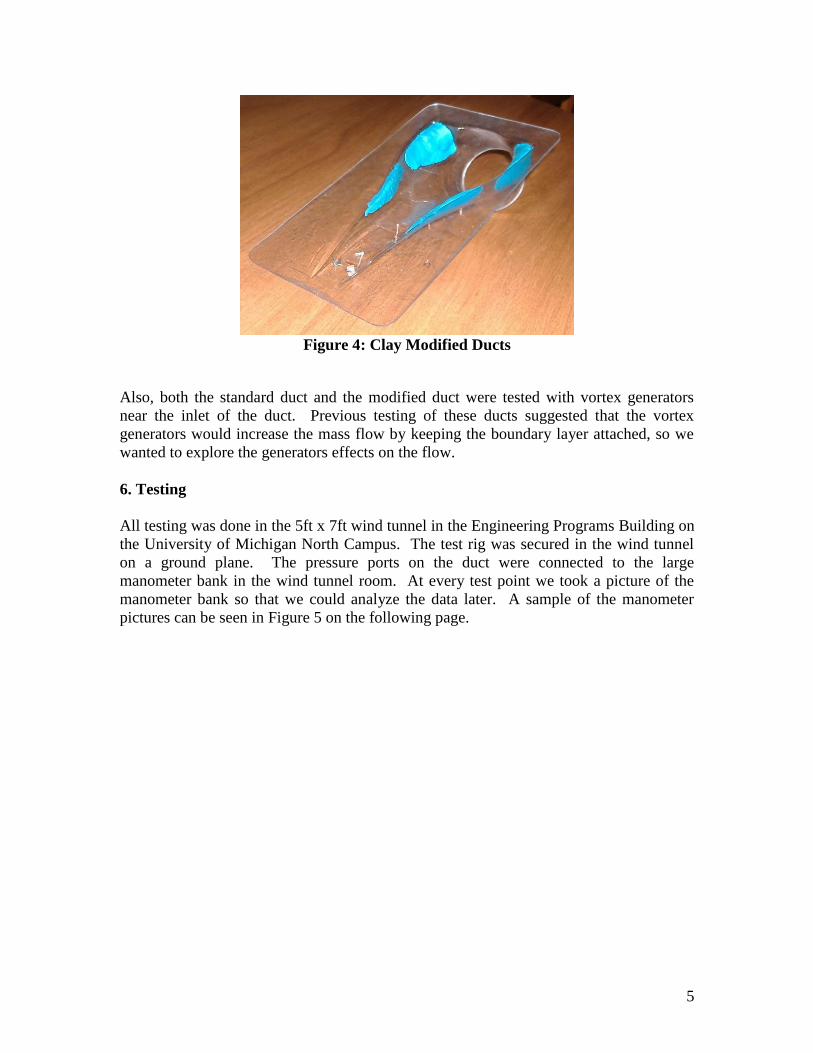
These depressions were filled in with clay to smooth out the surface to allow the flow to

go directly into the tube. These modifications can be seen in Figure 4.

5

Figure 4: Clay Modified Ducts

Also, both the standard duct and the modified duct were tested with vortex generators

near the inlet of the duct. Previous testing of these ducts suggested that the vortex

generators would increase the mass flow by keeping the boundary layer attached, so we

wanted to explore the generators effects on the flow.

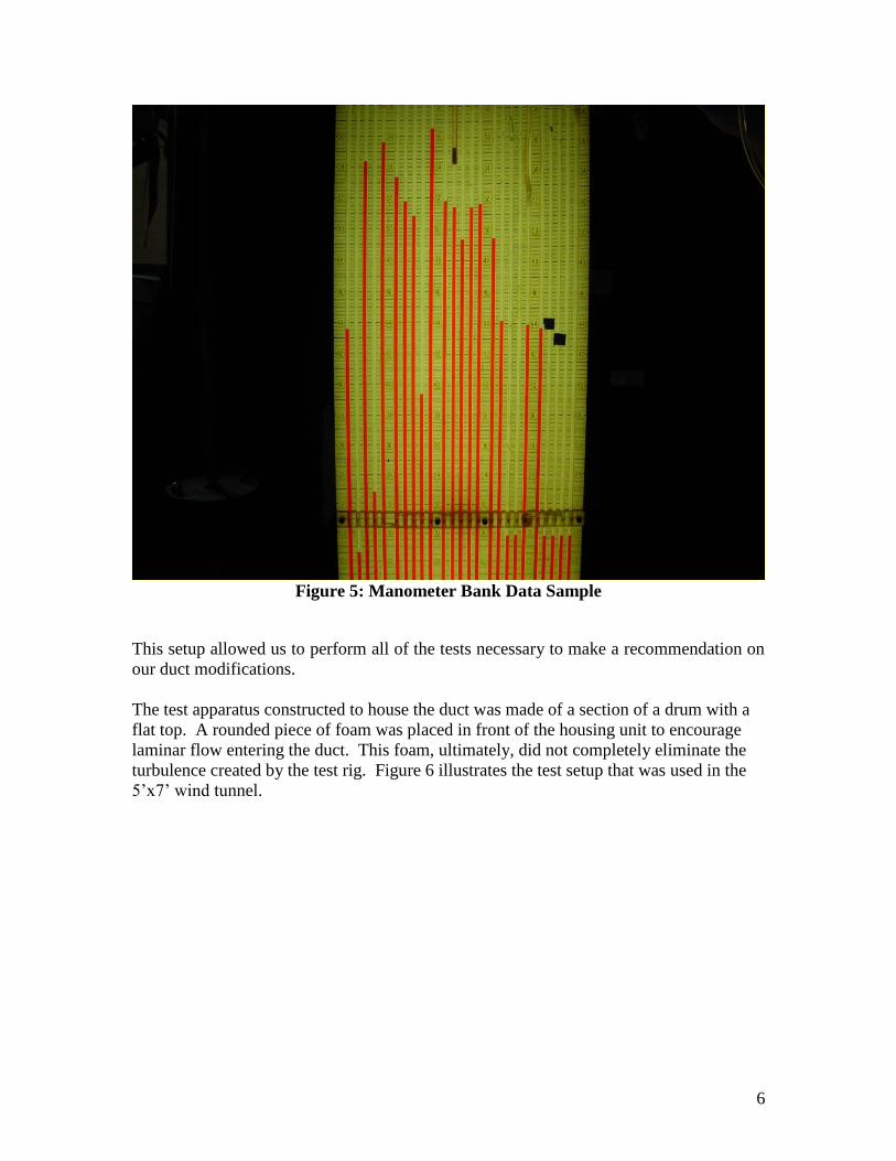
6. Testing

All testing was done in the 5ft x 7ft wind tunnel in the Engineering Programs Building on

the University of Michigan North Campus. The test rig was secured in the wind tunnel

on a ground plane. The pressure ports on the duct were connected to the large

manometer bank in the wind tunnel room. At every test point we took a picture of the

manometer bank so that we could analyze the data later. A sample of the manometer

pictures can be seen in Figure 5 on the following page.

6

Figure 5: Manometer Bank Data Sample

This setup allowed us to perform all of the tests necessary to make a recommendation on

our duct modifications.

The test apparatus constructed to house the duct was made of a section of a drum with a

flat top. A rounded piece of foam was placed in front of the housing unit to encourage

laminar flow entering the duct. This foam, ultimately, did not completely eliminate the

turbulence created by the test rig. Figure 6 illustrates the test setup that was used in the

5’x7’ wind tunnel.

7

Figure 6: Test apparatus for NACA duct testing in wind tunnel

The duct was placed flush with the top of the drum, parallel to the flow stream. Smooth,

flat tape was used to secure the duct to the top of the apparatus. Pressure ports were

placed along the inside of the duct to measure the static pressure of the flow. A flexible

tube was secured to the outlet of the duct inside of the apparatus and passed through the

opening in the back of the apparatus as shown in Figure 7.

Figure 7: Exit Tube

8

Figure 8 below shows the arrangement of the pressure ports along the side of the duct.

Figure 8: Pressure ports along the side of NACA duct

The radial pitot rake was placed inside of this flexible pipe, about six inches downstream

of the outlet of the duct. The pitot rake was used to measure total pressure. These

pressure measurements were then used to determine the mass flow rate through the duct.

This pitot rake can be seen in Figure 9 below. Two static ports we also incorporated into

the duct and we located at ports 11 and 12. A detailed schematic can be seen in

Appendix C.

Figure 9: Radial pitot rake at the outlet of NACA duct

The entire apparatus was secured to the ground plane inside of the wind tunnel with bolts

during testing. The ground plane was paramount in the testing of the performance of the

NACA ducts during the yaw test due to its ability to be rotated to a predetermined angle.

7. Results

Using the previously described test set-up in section 6.1 our team tested two ducts with

two different configurations. Figures 10-12 display the volumetric flow (V) versus the

speed of the air (s) given in standard cubic feet per minute (scfm) versus miles per hour

(mph). Using the program in Appendix A, we were able to calculate various

characteristics of the flow. Not all of these characteristics are included because they were

9

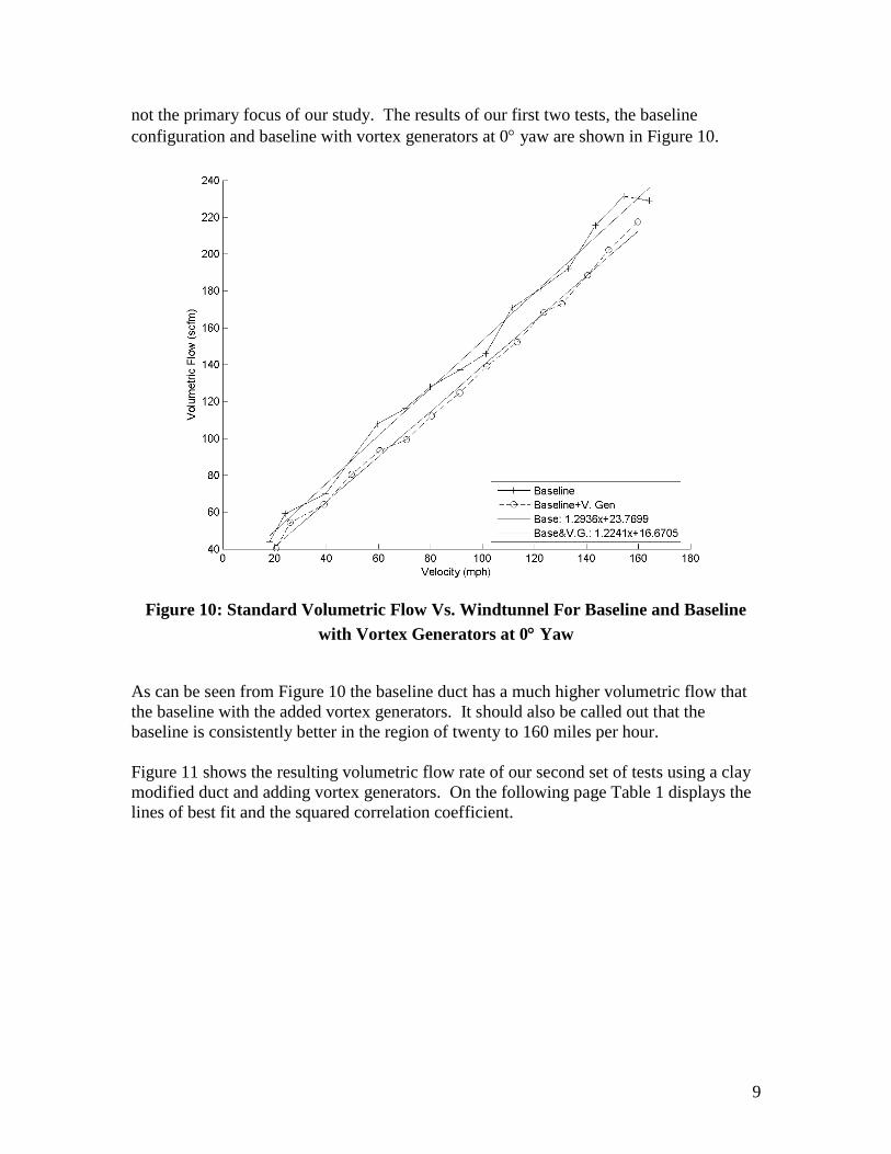
not the primary focus of our study. The results of our first two tests, the baseline

configuration and baseline with vortex generators at 0 yaw are shown in Figure 10.

Figure 10: Standard Volumetric Flow Vs. Windtunnel For Baseline and Baseline

with Vortex Generators at 0 Yaw

As can be seen from Figure 10 the baseline duct has a much higher volumetric flow that

the baseline with the added vortex generators. It should also be called out that the

baseline is consistently better in the region of twenty to 160 miles per hour.

Figure 11 shows the resulting volumetric flow rate of our second set of tests using a clay

modified duct and adding vortex generators. On the following page Table 1 displays the

lines of best fit and the squared correlation coefficient.

10

Figure 11: Standard Volumetric Flow Vs. Windtunnel For Clay Modified and Clay

Modified with Vortex Generators at 0 Yaw

Again in this test we found that vortex generators hinder the amount of flow passing

through the ducts. However, compared to the baseline duct we see a substantial increase

in mass flow for the clay modified duct, on the order of 37.3% at approximately 142

miles per hour. This is better visualized using Figure 12 on the next page, a plot of the

baseline and clay modified ducts.

One major feature of the results is the linearity in the region of twenty to 160 miles per

hour. As can be seen visually, and mathematically though the correlation coefficient

close to 1, a linear fit is outstanding for this region. There are obvious non-linear effects

as the velocity goes to zero because at zero, there can be no flow through the duct.

Test

Line of Best Fit

V(scfm)=f(mph) R²

Baseline 1.2936 23.7699V s 0.992

Baseline & V.G. 1.2241 16.6705V s 0.996

Clay Modification 2.0178 11.1658V s 0.983

Clay Modification & V.G. 1.879 2.1669V s 0.999

Table 5: Line of Best Fit for Individual Tests

11

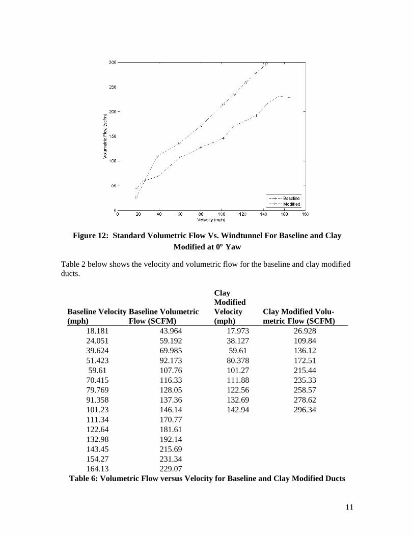
Figure 12: Standard Volumetric Flow Vs. Windtunnel For Baseline and Clay

Modified at 0 Yaw

Table 2 below shows the velocity and volumetric flow for the baseline and clay modified

ducts.

Baseline Velocity

(mph)

Baseline Volumetric

Flow (SCFM)

Clay

Modified

Velocity

(mph)

Clay Modified Volu-

metric Flow (SCFM)

18.181 43.964 17.973 26.928

24.051 59.192 38.127 109.84

39.624 69.985 59.61 136.12

51.423 92.173 80.378 172.51

59.61 107.76 101.27 215.44

70.415 116.33 111.88 235.33

79.769 128.05 122.56 258.57

91.358 137.36 132.69 278.62

101.23 146.14 142.94 296.34

111.34 170.77

122.64 181.61

132.98 192.14

143.45 215.69

154.27 231.34

164.13 229.07

Table 6: Volumetric Flow versus Velocity for Baseline and Clay Modified Ducts

12

As mentioned before the clay modified ducts appear to be far better due to the rounding

of the back corners and narrowing of the inlet aperture. Following the baseline tests for

our ducts, we then changed the yaw angle of our test apparatus to determine the effect on

volumetric flow. The results are surprising to say the least. As the yaw angle is

increased, the more mass flow the driver receives. This can be seen in Figure 13.

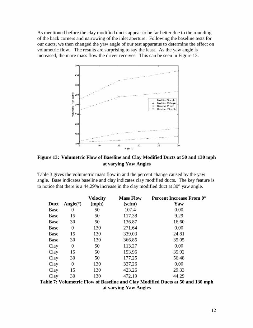
Figure 13: Volumetric Flow of Baseline and Clay Modified Ducts at 50 and 130 mph

at varying Yaw Angles

Table 3 gives the volumetric mass flow in and the percent change caused by the yaw

angle. Base indicates baseline and clay indicates clay modified ducts. The key feature is

to notice that there is a 44.29% increase in the clay modified duct at 30 yaw angle.

Duct Angle(°)

Velocity

(mph)

Mass Flow

(scfm)

Percent Increase From 0°

Yaw

Base 0 50 107.4 0.00

Base 15 50 117.38 9.29

Base 30 50 136.87 16.60

Base 0 130 271.64 0.00

Base 15 130 339.03 24.81

Base 30 130 366.85 35.05

Clay 0 50 113.27 0.00

Clay 15 50 153.96 35.92

Clay 30 50 177.25 56.48

Clay 0 130 327.26 0.00

Clay 15 130 423.26 29.33

Clay 30 130 472.19 44.29

Table 7: Volumetric Flow of Baseline and Clay Modified Ducts at 50 and 130 mph

at varying Yaw Angles

13

8. Conclusions and Recommendations

Overall we were very pleased with the results we obtained from testing. Our data had

good linear trends so this makes it easy to make any predictions for higher speeds if

needed in the future. We saw vast improvement in mass flow with the modifications that

were tested. Our results show that there is a 145.8% increase in volumetric flow with the

clay modifications over the standard NACA duct we used as our baseline.

Based on these results it is our recommendation to use the duct with clay modifications

and angle the duct at 30 degrees on the side of the car. If further work is to be done, we

recommend dimpling the ramp to create vortex generators without obstructing the flow.

Last year’s group did find that vortex generator did help keep the flow attached and

lowered the boundary layer though we found that the vortex generators they were using

hindered the flow. Also more testing regarding the yaw angle would be advisable since

we had such large incremental gaps in our testing angles.

9. Omissions

One thing we wanted to do but were unable due to software and time constraints was to

make a Computer Aided Design (CAD) model import it into Computational Fluid

Dynamic (CFD) software. We wanted to do this to look at theoretical data and to see

how our close our test results came to theoretical numbers. Since the geometry of the

ducts is very complex it was difficult to make an accurate model. We did try a laser scan

to create a file that could be used as a CAD model to import into CFD software. The

software did not like our model and did not create a good mesh in order to do any

simulations. If future work is done, CFD analysis should be done but work on these need

to be started earlier in order to compensate all the unforeseen problems with the software.

14

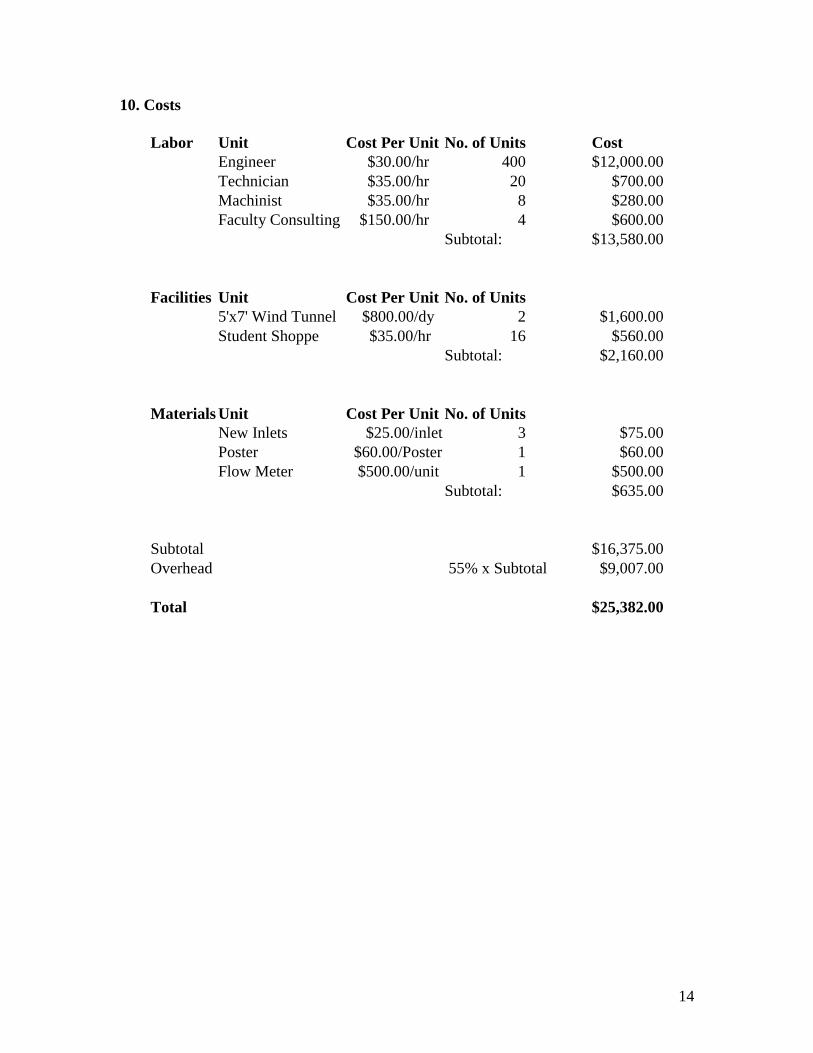
10. Costs

Labor Unit Cost Per Unit No. of Units Cost

Engineer $30.00/hr 400 $12,000.00

Technician $35.00/hr 20 $700.00

Machinist $35.00/hr 8 $280.00

Faculty Consulting $150.00/hr 4 $600.00

Subtotal: $13,580.00

Facilities Unit Cost Per Unit No. of Units

5'x7' Wind Tunnel $800.00/dy 2 $1,600.00

Student Shoppe $35.00/hr 16 $560.00

Subtotal: $2,160.00

Materials Unit Cost Per Unit No. of Units

New Inlets $25.00/inlet 3 $75.00

Poster $60.00/Poster 1 $60.00

Flow Meter $500.00/unit 1 $500.00

Subtotal: $635.00

Subtotal $16,375.00

Overhead 55% x Subtotal $9,007.00

Total $25,382.00

15

11. Schedule

Figure 1414: Gantt Chart

16

12. Bibliography

Anderson, John. (2007). Fundamentals of Aerodynamics (4th

ed). Boston: McGraw

Hill.

Bairstow, Leonard. (1920). Applied Aerodynamics (1st ed.). London: Longmans and

Company.

Brown, James Ward, & Churchill, Ruel. (2003). Complex Variables and Applications

(7th

ed). Boston: McGraw Hill.

Chow, Cheun-Yen, & Keuthe, Arnold M. (1976). Foundations of Aerodynamics (3rd

ed).

New York: Wiley.

Milne-Thomson, L. M. (1973). Theoretical Aerodynamics (4th

ed). New York: Dover.

United States. National Advisory Committee for Aeronautics. Katzoff, S. (December

1940). The Design of Cooling Ducts with Special Reference to the Boundary

Layer at the Inlet. Langley Field, Virginia. NACA.

United States. National Advisory Committee for Aeronautics. Czarnecki, K.R., &

Nelson, W.J. (September 1943). Wind-Tunnel Testing of Rear Underslung

Fuselage Ducts. Langley Field, Virginia. NACA.

United States. National Advisory Committee for Aeronautics. Mossman, Emmet, &

Randall, Lauros. (January 1948). An Experimental Investigation of the Design

Variables for NACA Submerged Duct Entrances. Langley Field, Virginia. NACA.

17

Appendix A: Program

function pressuredata()

%{

port2man=xlsread('Port to Manometer.xls','A2:B20');

f=dir(fullfile('Picture Data','*.xls'));%Reads all the Microsoft Excel...

%file names in directory

s3=size(f);

cd('Picture Data')

data=struct('con',{},'P',{},'T',{},'D',{},'rho',{},'vtun',{},'run',...

{},'Pic',{},'ang',{});

%{

*.con=Test Number

*.P=Pressure

*.T=Temperature

*.D=Manometer Height

*.rho=Density

*.vtun=Free Stream Velocity

*.run=Data Point

*.Pic=Corresponding Picture

*.angle=Angle of Yaw

%}

for n=1:s3(1)

[d1]=xlsread(f(n).name,'Test Info','B1:B5');

data(n).con=d1(1);

data(n).P=d1(4);

data(n).T=d1(5)+459.67;

[num txt raw]=xlsread(f(n).name,'Data');

data(n).run=num(:,1);

data(n).Pic=num(:,23);

data(n).ang=num(:,24);

data(n).D=[num(:,2) num(:,3) num(:,port2man(:,2)'+1)];

data(n).vtun=.3048*14.439*sqrt((data(n).D(:,1)-data(n).D(:,2))*...

data(n).T/data(n).P);

data(n).P=d1(4)*3386;

data(n).T=(d1(5)+459.67)/1.8;

data(n).rho=data(n).P/(286.9*data(n).T);

clear('num','d1','txt','raw')

end

cd ..

save('WTdata','data')

%}

load('WTdata.mat')

18

psp=[2 3 4 5 6 7 8 11 12]+1;%Static Pressure Ports

pspb=[11]+1;%Static Pressure Port Bottom

ptpb=[13 14 15 16 20]+1;%Bottom Total Pressure Ports

pspt=[12]+1;%Top Static Port

ptpt=[17 17 17]+1;%Top Total Pressure Ports

ptp=[13:20]+1;%Total Pressure Ports

value=struct('pspvel',{},'psp',{},'ptpvel',{},'ptp',{},'pres',{},...

'vel',{},'mfr',{},'scfm',{});

%{

*.pspvel=Static Pressure Port Velocity

*.psp=Manometer Difference Static Pressure Port

*.ptpvel=Total Pressure Ports Velocity

*.ptp=Manometer Difference Total Pressure Port

*.pres=Pressure At Port

*.vel=Velocity At Port

*.mfr=Mass Flow Rate

*.scfm=Standard Cubic Feet Per Minute (SI STP)

%}

for a=1:6

value(a).pspvel=.3048*14.439*sqrt((data(a).P-data(a).D(:,psp))*...

1.8*data(a).T/(data(a).P/3384));

s1=size(data(a).D(:,ptpb));

for b=1:s1(2)

value(a).ptpvel(:,b)=[.3048*14.439*sqrt(-(data(a).D(:,ptpb(b))-...

data(a).D(:,pspb))*1.8*data(a).T/(data(a).P/3384))];

value(a).ptp(:,b)=data(a).D(:,ptpb(b))-data(a).D(:,pspb);

end

s2=size(ptpt);

for c=1:s2(2)

value(a).ptpvel(:,c+5)=[.3048*14.439*sqrt(-(data(a).D(:,ptpt(c))-...

data(a).D(:,pspb))*1.8*data(a).T/(data(a).P/3384))];

value(a).ptp(:,c+5)=data(a).D(:,ptpb(c))-data(a).D(:,pspb);

end

value(a).ptpvel=value(a).ptpvel(:,[[1:4] [6:8] 5]);

value(a).ptp=value(a).ptp(:,[[1:4] [6:8] 5]);

value(a).vel=[value(a).pspvel value(a).ptpvel];

value(a).mfr=sum(value(a).ptpvel*3.683^2*pi/8*data(a).rho,2);

value(a).psp=data(a).P-data(a).D(:,psp);

value(a).scfm=value(a).mfr*data(a).P/101325*273.15/data(a).T*...

3.53146667E-5*3600;

%{

figure(a)

plot(data(a).vtun,value(a).mfr,'k+')

19

xlabel('Velocity (m/s)')

ylabel('Volumetric Flow (cc/s)')

%}

end

%{

figure(1)

plot(data(1).vtun,value(1).mfr,'k+-',data(2).vtun,value(2).mfr,'ko--')



title('Baseline Duct Volumetric Flow vs. Tunnel Velocity')

legend('Baseline','Baseline+V. Gen','Location','SE')

figure(2)

plot(data(3).vtun,value(3).mfr,'k+-',data(4).vtun,value(4).mfr,'ko--')



title('Modified Duct Volumetric Flow vs. Tunnel Velocity')

legend('Modified','Modified+V. Gen','Location','SE')

figure(3)

plot(data(5).ang(1:3),value(5).mfr(1:3),'k+--',data(5).ang(4:6),...

value(5).mfr(4:6),'k^--',data(6).ang(1:3),value(6).mfr(1:3),...

'ko--',data(6).ang(4:6),value(6).mfr(4:6),'kv--')

xlabel('Angle (\circ)')


title('Volumetric Flow for Baseline and Modified Ducts')

legend('Modified 50 mph','Modified 130 mph','Baseline 50 mph',...

'Baseline 130 mph','Location','E')

%}

%%{

figure(4)

[coef r1]=fit(2.2369*data(1).vtun,value(1).scfm,'poly1');

c1=[coef.p1 coef.p2]

r1



r2

hold on

plot(2.2369*data(1).vtun,value(1).scfm,'k+-',2.2369*data(2).vtun,...

value(2).scfm,'ko--')

plot(2.2369*data(1).vtun,polyval(c1,2.2369*data(1).vtun),'k',...

2.2369*data(2).vtun,polyval(c2,2.2369*data(2).vtun),'k')

xlabel('Velocity (mph)')

ylabel('Volumetric Flow (scfm)')

%title('Baseline Duct Volumetric Flow vs. Tunnel Velocity')

legend('Baseline','Baseline+V. Gen',['Base: ' num2str(c1(1)) ...

20

'x+' num2str(c1(2))],['Base&V.G.: ' num2str(c2(1)) 'x+'

num2str(c2(2))],'Location','SE')

saveas(gcf,'baseline','tif')

figure(5)



r3



r4

hold on

plot(2.2369*data(3).vtun,value(3).scfm,'k+-',2.2369*data(4).vtun,...


plot(2.2369*data(3).vtun,polyval(c3,2.2369*data(3).vtun),'k',...

2.2369*data(4).vtun,polyval(c4,2.2369*data(4).vtun),'k')



%title('Clay Modified Reduced Inlet: Volumetric Flow vs. Tunnel Velocity')

legend('Modified','Modified+V. Gen',['Mod: ' num2str(c3(1)) 'x+' ...

num2str(c3(2))],['Mod&V.G.: ' num2str(c4(1)) 'x+'...

num2str(c4(2))],'Location','SE')

saveas(gcf,'modified','tif')

figure(6)

plot(data(5).ang(1:3),value(5).scfm(1:3),'k+--',data(5).ang(4:6),...

value(5).scfm(4:6),'k^--',data(6).ang(1:3),value(6).scfm(1:3),...

'ko--',data(6).ang(4:6),value(6).scfm(4:6),'kv--')

xlabel('Angle (\circ)')


%title('Yaw Tests For Volumetric Flow for Baseline and Modified Ducts')

legend('Modified 50 mph','Modified 130 mph','Baseline 50 mph',...

'Baseline 130 mph','Location','E')

saveas(gcf,'yaw','tif')

figure(7)

plot(2.2369*data(1).vtun,value(1).scfm,'k+--',2.2369*data(3).vtun,...




%title('Baseline vs. Clay Modified Reduced Inlet: Volumetric Flow...

%vs. Tunnel Velocity')

legend('Baseline','Modified','Location','SE')

saveas(gcf,'basevsmod','tif')

%}

save('testdat.mat','value')

21

Appendix B: Data

Test Information:

Test 1

Duct Baseline

Date 10-Mar-08

Pressure 29.459 inHg

Tunnel Temperature 42.7 F

Test 2

Duct Baseline + Vortex Generators

Date 10-Mar-08

Pressure 29.459 inHg

Tunnel Temperature 56.5 F

Test 3

Duct Modified

Date 11-Mar-08

Pressure 29.142 inHG

Tunnel Temperature 26 F

Test 4

Duct Modified + Vortex Generators

Date 11-Mar-08



Test 5

Duct Modified Angular

Date 11-Mar-08



Test 6

Duct Baseline Angular

Date 11-Mar-08



22

Test 1: Data - Baseline

Test 2: Data – Baseline and Vortex Generators

Test 3: Data – Clay Modified

23

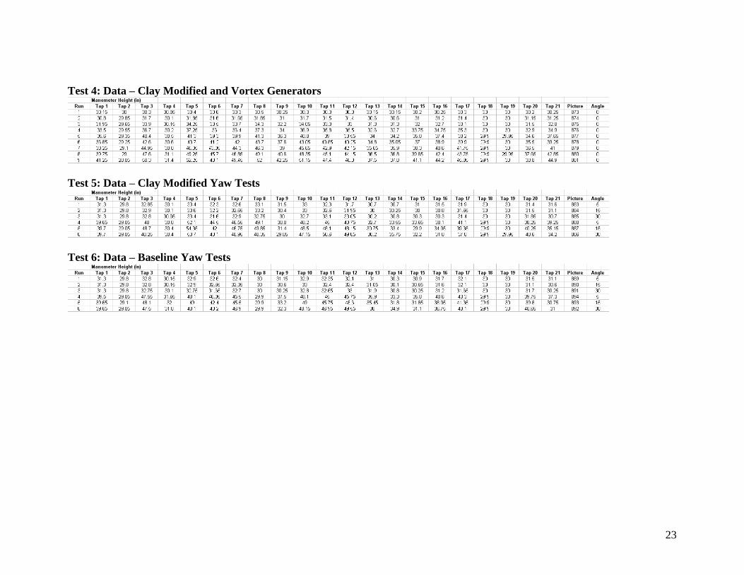
Test 4: Data – Clay Modified and Vortex Generators

Test 5: Data – Clay Modified Yaw Tests

Test 6: Data – Baseline Yaw Tests

25

Appendix C: Final Pitot Configuration

Figure 15: Pitot Static Ports Numbering Scheme

Pressure

Port

Manometer

Tap

2 10

3 3

4 4

5 5

6 6

7 7

8 8

9 9

10 21

11 11

12 12

13 13

14 14

15 15

16 16

17 17

18 18

19 19

20 20

Table 8: Pitot Tube to Manometer Port

3

5

11

7

2 4 6 8

9

9

12

10

9

26

Figure 16: Pitot Total Pressure Ports Numbering Scheme

Static pressure port

Static pressure port

19 18

20

13

14

15

16

17

Table of Contents - University of Michiganriboch/publications/NACADuct.pdf · Table of Contents...

Documents

Transcript of Table of Contents - University of Michiganriboch/publications/NACADuct.pdf · Table of Contents...