TABLE OF CONTENTS - Teledyne LeCroycdn.teledynelecroy.com/files/manuals/lw400a-om2.pdfCAUTION: Refer...

1

TABLE OF CONTENTS

Arbitrary Waveform Generator Users Guide

1. General

Installation and Safety . . . . . . . . . . . . . . . . . . . . . . . . . .13

Getting Started . . . . . . . . . . . . . . . . . . . . . . . . . . . . . . . .18

2. Introductory Tutorial

Creating a simple Arbitrary Waveform . . . . . . . . . . . . . . .21

3. Waveform Viewing

Waveform Selection . . . . . . . . . . . . . . . . . . . . . . . . . . . .33

Display Setup . . . . . . . . . . . . . . . . . . . . . . . . . . . . . . . . .37

Zooming . . . . . . . . . . . . . . . . . . . . . . . . . . . . . . . . . . . .310

4. Live Waveform Manipulation

Time Cursors . . . . . . . . . . . . . . . . . . . . . . . . . . . . . . . . .41

Voltage Cursors . . . . . . . . . . . . . . . . . . . . . . . . . . . . . . .43

Edit Time . . . . . . . . . . . . . . . . . . . . . . . . . . . . . . . . . . . .45

Duration . . . . . . . . . . . . . . . . . . . . . . . . . . . . . . . . . . . . .45

Move Feature . . . . . . . . . . . . . . . . . . . . . . . . . . . . . . . . .46

Delay . . . . . . . . . . . . . . . . . . . . . . . . . . . . . . . . . . . . . . .46

Edit Amplitude . . . . . . . . . . . . . . . . . . . . . . . . . . . . . . . .48

5. Insert Wave

From Scope . . . . . . . . . . . . . . . . . . . . . . . . . . . . . . . . . .52

Standard Waves . . . . . . . . . . . . . . . . . . . . . . . . . . . . . . .54

Equations . . . . . . . . . . . . . . . . . . . . . . . . . . . . . . . . . . . .57

Other Waves . . . . . . . . . . . . . . . . . . . . . . . . . . . . . . . . .526

6. Waveform Editing

Clearing the Display . . . . . . . . . . . . . . . . . . . . . . . . . . . .61

Editor Properties and Options . . . . . . . . . . . . . . . . . . . . .63

Insert . . . . . . . . . . . . . . . . . . . . . . . . . . . . . . . . . . . . . . .65

Cut . . . . . . . . . . . . . . . . . . . . . . . . . . . . . . . . . . . . . . . .66

Paste . . . . . . . . . . . . . . . . . . . . . . . . . . . . . . . . . . . . . . .69

2

Table of Contents

7. Sequence Waveforms

Sequence Editor . . . . . . . . . . . . . . . . . . . . . . . . . . . . . . .73

Sequence Example . . . . . . . . . . . . . . . . . . . . . . . . . . . . .75

Group Sequences . . . . . . . . . . . . . . . . . . . . . . . . . . . . .711

8. Waveform Math

Dual Waveform Math . . . . . . . . . . . . . . . . . . . . . . . . . . .88

Example . . . . . . . . . . . . . . . . . . . . . . . . . . . . . . . . . . . . .88

9. Adding Noise to A Waveform

Adding noise on the LW400/LW400A . . . . . . . . . . . . . . . . .93

Adding Noise on the LW400B . . . . . . . . . . . . . . . . . . . . . . .93

Controlling Noise . . . . . . . . . . . . . . . . . . . . . . . . . . . . . . . .94

10. Project Structure

Project Import . . . . . . . . . . . . . . . . . . . . . . . . . . . . . . . . . .105

Project Export . . . . . . . . . . . . . . . . . . . . . . . . . . . . . . . . . .107

11. Hardcopy

Printers . . . . . . . . . . . . . . . . . . . . . . . . . . . . . . . . . . . .113

Storing Graphics Files . . . . . . . . . . . . . . . . . . . . . . . . . .114

File Naming . . . . . . . . . . . . . . . . . . . . . . . . . . . . . . . . .115

12. Importing & Exporting Waveform Files

Spreadsheet . . . . . . . . . . . . . . . . . . . . . . . . . . . . . . . .129

MathCad . . . . . . . . . . . . . . . . . . . . . . . . . . . . . . . . . .1210

PSpice . . . . . . . . . . . . . . . . . . . . . . . . . . . . . . . . . . . .1212

MatLab . . . . . . . . . . . . . . . . . . . . . . . . . . . . . . . . . . .1213

EasyWave File . . . . . . . . . . . . . . . . . . . . . . . . . . . . . .1215

LeCroy Scope File . . . . . . . . . . . . . . . . . . . . . . . . . . . .1216

Other Files . . . . . . . . . . . . . . . . . . . . . . . . . . . . . . . . .1217

Exporting Files . . . . . . . . . . . . . . . . . . . . . . . . . . . . . .1218

3

Table of Contents

13. Setting the Clock

LW400 Clock . . . . . . . . . . . . . . . . . . . . . . . . . . . . . . . . . . .132

LW400A/B Clock . . . . . . . . . . . . . . . . . . . . . . . . . . . . . . . .136

External ReferenceSynchronization . . . . . . . . . . . . . . .139

14. Marker

Programming the Marker . . . . . . . . . . . . . . . . . . . . . . . .142

Clocking with the Marker . . . . . . . . . . . . . . . . . . . . . . . .144

15. Trigger

Trigger Setup . . . . . . . . . . . . . . . . . . . . . . . . . . . . . . . . . . .151

16. Interfaces

Centronics . . . . . . . . . . . . . . . . . . . . . . . . . . . . . . . . . .162

GPIB . . . . . . . . . . . . . . . . . . . . . . . . . . . . . . . . . . . . . .163

17. Function Generator

Standard Functions . . . . . . . . . . . . . . . . . . . . . . . . . . . . . .172

18. Disk Utilites

Floppy Disk . . . . . . . . . . . . . . . . . . . . . . . . . . . . . . . . . . . .181

Hard Disk . . . . . . . . . . . . . . . . . . . . . . . . . . . . . . . . . . . . . .182

Appendix A: Measurement Functions Description

Appendix B: WaveStation Specifications

Appendix C: LW400-09A Digital Output Option

1-1

GENERAL INFORMATION

Warranty LeCroy warrants operation under normal use for a period of oneyear from the date of shipment. Replacement parts and repairsare warranted for 90 days. Accessory products not manufacturedby LeCroy are covered by the original equipment manufacturerswarranties.

In exercising this warranty, LeCroy will repair or, at its option,replace any product returned to the factory or an authorized servicefacility within the warranty period only if the warrantors examina-tion discloses that the product is defective due to workmanship ormaterials and the defect has not been caused by misuse, neglect,accident, or abnormal conditions or operations.

The purchaser is responsible for transportation and insurancecharges. LeCroy will return all in-warranty products with transporta-tion prepaid.

This warranty is in lieu of all other warranties, express or implied,including but not limited to any implied warranty of merchantability,fitness, or adequacy for any particular purpose or use. LeCroyCorporation shall not be liable for any special, incidental, or conse-quential damages, whether in contract or otherwise.

Product Assistance Help with installation, calibration, and the use of LeCroy productsis available from your local LeCroy office or a LeCroy customerservice center.

Maintenance Agreements LeCroy offers a choice of customer support services to meet yourindividual needs. Extended warranty maintenance agreements letyou budget maintenance costs after the initial warranty hasexpired. Other services such as installation, training, calibration,enhancements and on-site repair are available through specificSupplemental Support Agreements. Contact your local LeCroyoffice or a LeCroy customer service center for details.

1

RETURN A PRODUCTFOR SERVICE OR REPAIR If you do need to return a LeCroy product, identify it for us using

both its model and serial numbers (see rear of instrument).Describe the defect or failure, and provide your name and contactnumber. For factory returns, use a Return Authorization Number(RAN), obtainable from customer service. Attach it so that it can beclearly seen on the outside of the shipping package to ensurerapid redirection within LeCroy. Return those products requiringonly maintenance to your customer service center.

Within the warranty period, transportation charges to the factorywill be your responsibility, while all in-warranty products will bereturned to you with transport prepaid by LeCroy. Outside thewarranty period, you will have to provide us with a purchase-ordernumber before the work can be done. And you will be billed forparts and labor related to the repair work, as well as for shipping.

You should pre-pay return shipments. LeCroy cannot accept COD(Cash On Delivery) or Collect Return shipments. We recommendusing air-freight.

TIP: If you need to return your WaveStation, try to use the originalshipping carton. If this is not possible, the carton used should berigid and be packed so that that the product is surrounded by aminimum of four inches, or 10 cm, of shock-absorbent material.

Software Upgrades To determine the software revision presently installed:

1) press 2nd then soft key on the front panel.

2) press Page Down

3) observe SW Rev: line on the display

To update Revision: 1) Turn off instrument power

2) Insert floppy disk

3) Power on instrument and the firmware will be updated

1-2

General Information

1-3

Installation and Safety

Operating Environment The WaveStation will operate to its specifications if the environ-ment is maintained within the following parameters:

Temperature: 5° to 35° C to full specifications, 0° to 40° C operating, -20° to 70° Cnon-operating

Humidity: 10% to 80% non-condensingAltitude: < 2000 Meters (6560 ft)Operation: Indoor use only

This equipment complies to Safety Standards per EN 61010-1(Safety Requirements for Electrical Equipment for Measurement,Control, and Laboratory Use). It has been been qualified to thefollowing EN 61010-1 categories:

Installation (Overvoltage) Category IIPollution Degree 2.

Safety Symbols Where these symbols or indications appear on the front or rearpanels, and in this manual, they have the following meanings:

CAUTION: Refer to accompanying documents (for Safety-relatedinformation). See elsewhere in this manual wherever the symbol ispresent, as indicated in the Table of Contents.

On (Supply) Off (Supply)

Alternating Current Only CAUTION, Risk of electric shock

Protective Conductor Terminal Earth Terminal

WARNING Denotes a hazard. If a WARNING is indicated on the instrument,do not proceed untils its conditions are understood and met.

x

~

1-4

Any use of this instrument in a manner not specified by themanufacturer may impair the instruments safety protection.

The WaveStation has not been designed for use in making directmeasurements on the human body. Users who connect aWaveStation directly to a person do so at their own risk.

Power Requirements The WaveStation operates from a 115 V (90 to 132 V) or 230 V(180 to 250 V) AC (~) power source at 47 Hz to 63 Hz. Novoltage selection is required, since the instrument automaticallyadapts to the line voltage present.

The power supply of the WaveStation is protected against short-circuit and overload by means of one internal 5.0A/250 V ~, "T" rated fuse. The fuse is not replaceable by the user.

The WaveStation has been designed to operate from a single-phase power source, with one of the current-carrying conductors(neutral conductor) at ground (earth) potential. Maintain the groundline to avoid an electric shock.

None of the current-carrying conductors may exceed 250 V rmswith respect to ground potential. The WaveStation is provided witha three-wire electrical cord containing a three-terminal polarizedplug for mains voltage and safety ground connection. The plug'sground terminal is connected directly to the frame of the unit. Foradequate protection against electrical hazard, this plug must beinserted into a mating outlet containing a safety ground contact.

Power On Connect the WaveStation to the power outlet and switch it on bypressing the power switch located on the front panel. After theinstrument is switched on, a self test is peformed. The full testingprocedure takes approximately 30 seconds, after which time adisplay will appear on the screen.

Do not exceed the maximum specified input voltage levels. (Seeappendix B for details.)

Warning


1-5


Risk of electrical shock: No user serviceable parts inside. Leaverepair to qualified personnel.

Cleaning And Maintenance Maintenance and repairs should be carried out exclusively by aLeCroy technician. Cleaning should be limited to the exterior of theinstrument only, using a damp, soft cloth. Do not use chemicals orabrasive elements. Under no circumstances should moisture beallowed to penetrate the WaveStation. To avoid electric shocks,disconnect the instrument from the power supply before cleaning.

Service Procedure Refer any servicing requiring removal of exterior enclosure panelsto qualified LeCroy service personnel. Be prepared to describe theproblem in detail. Prior to returning a unit please obtain a ReturnAuthorization Number (RAN) from the LeCroy Customer Care Centerin New York at (914) 578-6020 or the LeCroy office nearest you.

If the product is under warranty, LeCroy will at its option, repair orreplace the LW400 Series at no charge. For repairs after thewarranty period, the customer must provide a Purchase OrderNumber before the service engineer can initiate repairs. Thecustomer will be billed for the parts, labor and shipping..

Shipping Guidelines 1. First attach a tag to the instrument which indicates:a. Return Authorization Numberb. Purchase Order numberc. Owners name and complete addressd. The service required including detailed operational problemse. Person to contact for confirmation (include phone number)

2. Ship the unit in its original packaging.3. Protect the finish by carefully wrapping the unit in polyethylene

sheeting.4. Place adequate dunnage or urethane foam in the container

(approximately 4 inch depth) and place the wrapped unit on it.Allow approximately four inches of space on all four sides andthe top of the unit.

5. Fasten the container with packaging tape and/or industrialstaples. Address the container to LeCroys service locationand include your return address.

CAUTION

1-6

Getting Started

How To Use This Manual

The LW400 Series arbitrary waveform generator is designed to beoperated without having to refer to this manual. This is madepossible by the intuitive controls and guiding menus. Most of thearbitrary waveform generator functions are accessed using theOperation Keys clustered around the rotary knob. The other pushbuttons give access to the useful new features offered by this inno-vative instrument. A built-in Help library is provided for instant aidin answering questions while operating the AWG.

It is suggested that this manual be used to:1. Gain an overview of the instrument2. Familiarize you with the terminology3. Provide detailed descriptions of the various functions4. Illustrate the use of the new features of the instrument

Perhaps the best way to use it is to read through the early sectionsand then browse through the later chapters in order to becomefamiliar with the LW400s capabilities. The Table of Contents isorganized so that you can find the right information by locating thethings you want to do.

*Note: The LW400 Series includes the LW420, LW420A, andLW420B dual channel and the LW410, LW410A, and LW410Bsingle channel arbitrary waveform generators (AWGs). At times thedesignation LW400 is used to describe features common to allmodels. At other times specific reference is made to the LW400Aand the LW400B Series.

WaveStation Arbitrary Waveform Generator The LeCroy LW400 makes it easy to create and edit waveforms

The LW400 combines complete on board word proccessor like cut,copy and paste, waveform editing with live waveform feature manip-ulation and waveform generation. Salient benefits include:

1. 100 psec feature placement resolution

2. 400 MS/s maximum sample clock for each channel

1-7

Getting Started

3. Sample Clock:

LW400 series sample clock rate is selectable within fivedecade ranges as describedsee chapter13

LW400A and the LW400B series sample clock is continuoslyvariable from 6 KHz to 400 MHz with a 1 Hz resolutionseechapter 13

4. 100 MHz analog bandwidth

5. Fast Switch Group Sequence mode switches waveforms in < 11 ms minimizing test execution time.

6. 1 channel (LW410/LW410A/LW410B) and 2 channel(LW420/LW420A/lw420B) versions

7. Live update of waveform output

8. Stand alone design, no PC required

9. Waveform Data formats for Spreadsheets, PSpice,MathCad, MatLab, ASCII, and others

10. Up to 1 megabyte of playback memory (256 k standard)

11. Hard Disk of >400 Mbyte standard

12. 3.5 DOS compatible floppy disk for waveforms, sequence,equators, and projects, file transfer and storage

13. GPIB

14. SCPI compatible command set

15. Centronics hard copy interfaces

16. Internal Asynchronous noise source on the LW400 andLW400A series (not available on the LW400B series).

1-8

Getting Started

Accessories Supplied This Operators ManualRemote Programmers ManualPower Cord for country of destinationProtective Front CoverFirmware Installation Disk

Available AccessoriesLS-RM Rackmount KitLS400-SM Service ManualLS-CART Oscilloscope CartLS-TRANS Hardshell Transit CaseLS-SOFT Softshell Carrying BagDC-GPIB 2 meter GPIB cable

OptionsLW420-ME2 1 Mbyte MemoryLW410-ME2 1 Mbyte MemoryLW400-HD1 >400 Mbyte HDDLW400-09A Digital Output

Organization This manual is organized by application topics (e.g.,VIEWING WAVE-FORMS and WAVEFORM EDITING) in order to provide rapid accessto those areas of most use. When specific information concerningthe operation of a particular push button or control is needed referto the index of this guide or use the LW400 built-in HELP facility.

Using the Front Panel Controls The LW400 Getting Started Guide, which follows, describes the

basic operation of the LW400 series arbitrary waveform generators.Use it interactively with the tutorial in section 2 for a fast introduc-tion to LW400 operations.

1-9

Getting Started

Welcome to the LeCroy WaveStation LW400 arbitrary waveformgenerator (AWG) Getting Started Guide. This guide offers a quickoverview of basic LW400 operations. The Getting Started Guide isintended for a fast introduction or a brief review, more completedetails are available in the following sections of the LW400Operators Manual.

The WaveStation ConceptThe WaveStation Concept is unique among arbitrary waveformgenerators in that it is designed to make waveform creation aninteractive process. Waveforms can be created and modifiedcontinually with an observable, live response at the outputs.

The best place to start when learning to use the LW400 is to lookat the conceptual block diagram, shown below.

Figure 1.2 Block Diagram

1-10

Central to the operation of an AWG is waveform creation and modi-fication. This operation is done in the WaveStations editor whichincludes 3 workspaces. The channel 1 and channel 2 edit work-spaces drive the respective outputs. The connection is direct andpermits live updates of the output as the waveform is changed.The scratch pad area is an off-line, utility edit workspace. The EDITcontrol group on the front panel provides access to operations inthe edit work spaces. Waveform selection, creation, and modifica-tion are all EDIT functions.

When a workspace is selected the current waveform contents aredisplayed on the internal CRT display. The VIEW control groupprovides control of the display parameters, time and voltagecursors, as well as hardcopy operations.

The output operations, like filtering and the addition of additivewhite noise, are controlled by the CHAN1 and CHAN2 controls.

The SAVE and PROJECT controls are used to move waveformsbetween the hard disk or floppy disk and the edit workspace. Inaddition to its waveform file management role PROJECT includescontrol of system related operations such as the real time clockand control of the remote interfaces.

Getting Started

1-11

Front Panel Controls

LW420 Front Panel Layout

*Note the front panel of the LW410/LW410A is similar to theLW420/LW420A except that all controls related to channel 2 areremoved.

Figure 1.3 Front Panel Layout

1-12

The LW400 WaveStation is a menu driven instrument. Push buttoncontrols on the front panel bring up related menus on the CRTdisplay. The LW400 is controlled through the selection and/orentry of the desired parameters in the menus.

1. The controls on the LW400 front panel aredivided into functionally related groups. Forexample:

The VIEW Group controls display related func-tions including hardcopy and the measurementof waveforms on the CRT Screen.

The EDIT Group controls waveform selection, editing, and modification.

The CHAN 1 and CHAN 2 buttons are used to controlthe channel related elements of the output such asturning channel output on or off, adding noise, orsetting the output channel bandwidth.

2. The rotary control knob is used to select menu itemsor to scroll through numeric parameters within amenu item. The DIGIT select buttons set the rate of change ofthe rotary knob by selecting the digit of the numeric value to bemodified.


DISPLAY

1-13

3. The numeric keypadallows precise entry ofnumeric data into menufields. Unit multiplier,enter keys p, n, µ, mENTER, k, and M areused to attach theappropriate unit multi-pliers to the valuesbeing entered.

4. Dedicated controls are permanently labeled to indicate theirfunction.

5. Dual function controls have a secondary function indicated bya red label printed above the control. The second function isaccessed by first pressing the red push button labeled 2NDand then pressing the desired button.

6. Information on the function of each front panel button is readilyavailable by pressing the Help button followed by the desiredbutton or softkey.

7. The functions of the Menu or Softkeys, locatedadjacent to the CRT display, are indicated by menulabels shown on the display.

8. The rotary knob symbol appearing adjacent to a softkeylabel, on the CRT, indicates that the parameterdescribed in the label may be varied using the rotary knob.

The keypads symbol appearing next to a softkey label, on theCRT, indicates that the parameter described in the label canbe entered or changed using the front panel numeric keypad.

9. Softkey labels with a shadow box effect, such as the Markerlabel in the figure above, have additional menu items behindthe label. Pressing the corresponding softkey again will list allthe choices for that item.


1-14

The LW400 Display The main elements of the LW400 CRT display are shown in thefigure below. The display annotation summarizes the current stateof the generator including the date and time. Hardcopy capabili-ties allow the CRT display to be saved to a printer, plotter, orgraphics file for notebooks or test procedure documentation.

The Display

Figure 1.4

Waveform Locator

Trigger Mode

1-15

Rear Panel Connections

Rear Panel Connections

Note: The digital output connectors for ECL and TTL are not presentif the LW400-09A Digital Output option is not installed.

1-16

Using the LW400 as aFunction Generator The LW400 includes a function generator mode offering

Sine, Square, Triangle, Ramp, Pulse, DC, and Multi-tonewaveforms. The frequency of the periodic waveforms canbe swept linearly or logarithmically using user enteredsweep rate, and start/stop frequencies.

1. Select the function generator mode by pressing thered 2nd button and then selecting the desiredchannel. The Function Gen menu will be displayedallowing the selection of desired waveform, ampli-tude, offset, start phase, and frequency by meansof the softkeys and/or numeric keypad.

2. Pressing the menu softkey labeled Sweep will alter-nately turn the frequency sweep on and off asindicated by the toggle switch icon. Pushing theSweep Param menu key allows control of thesweep parameters.

3. Pressing the Chan 1 (or 2) button on the frontpanel allows access to the CH1 (or 2) menu.

4. The channel 1 (or 2) output can be turned on or offusing the menu key labeled Output.

5. The bandwidth of either channels output can becontrolled in decade steps from 10 kHz to 100MHz. Bandwidth is automatically selected but theuser may choose to override this selection.

6. Gaussian white noise can be added to the signal as apercentage of the peak to-peak signal level.

LW400 as a Function Generator

1-17

Figure 1.5

Generating Arbitrary Waveforms From Existing Waveform Files

Arbitrary waveforms can be generated from an existing waveformfile or from a sequence of files described by a waveform sequence.The EDIT group on the front panel is used to select an existingwaveform and output it.

1. Depress the SELECT WAVE button in the EDIT group.

2. Press the menu key corresponding to the waveform label ineither Channel 1 or Channel 2. Use the rotary control knob toselect the desired waveform filename which will be displayed andsimultaneously output, as shown in figure 1.5. Its that simple!

3. The LED indicator next to the CHANNEL 1 (or 2) output connectoris green when the waveform is being ouput and red when it is off.To control the output press the CHAN1 (or 2) button.

4. Push the menu button labeled Output, in the CH1 menu, totoggle the channel 1 output on or off.

Generating Arbitrary Waveforms

1-18

Recalling Other Waveforms or Sequences

Waveform files and sequences are stored in the LW400s internalhard drive under a dual level file system characterized by a projectname and a waveform or sequence filename. This permits multipleusers to each have their own set of independent waveform files.To recall a specific waveform you have to select the project it hasbeen stored in and then the waveform or sequence filename.

1. Press the PROJECT button.

2. Push the button labeled Open in the PROJECTmenu to see the existing project names.

3. Use the rotary knob to select the desired project,then press the Accept menu key.

4. Use SELECT WAVE, as shown previously, to see the available waveforms.

Recalling Other Waveforms

1-19

Creating a New Arbitrary Waveform Using Standard Waveforms The LeCroy WaveStation LW400 offers many techniques for

creating arbitrary waveforms. They can be imported from oscillo-scopes, or common mathematics programs. They can be createdfrom built in libraries of standard waveforms, or from mathematicalequations. A full complement of waveform editing, modification,and array math capabilities allows existing waveforms to be usedas sources of new waveforms. Waveforms are created in thecurrently open project, instructions for creating a new project arefound in the following section.

1. Depress the SELECT WAVE button in theEDIT group.

2. Press the menu key marked NEW to create a new waveformname in either channel 1, or channel 2, or scratch pad.

3. Enter the desired waveform name, up to 14 characters long,then press the Accept softkey.

4. Press the front panel EDITbutton to access the wave-form and sequence editfunctions.

5. Press the softkey labeledInsert Wave to access thewaveform sources.

6. The Insert Wave menuallows the choice ofacquiring the waveform froma digital oscilloscope, usingthe standard waveslibraries, creating a wave-form from an equation, orinserting another waveform.

Creating a New Waveform

1-20

7. Press the menu key corresponding to the Standard Waveslabel. The LW400 will display a menu listing the standardwaveform library.

8. The Sine menu, typical of the standard wave-form setup menus, shows the waveformparameters that are available to control thestandard waveform.

Select the menu softkey adjacent to thedesired parameter and then use the rotaryknob or the numeric keypad to enter the valueneeded. After all the parameters have beenentered, press the Accept softkey to createthe waveform.

9. The LED indicator next to the CHANNEL 1 (or2) output connector is green when the wave-form is being output and red when it is off. To turn the outputon press the CHAN1 (or 2) button.

10. Push the menu button labeled Output, in the CH1 (or 2) menu,to toggle the channel 1 (2) ouput on or off.

Starting a New Project Projects provide individual work and storage areas,especially helpful when multiple users share theAWG. To create a new project:

1. Press the PROJECT button.

2. Press the NEW softkey to enter a new projectname, just as the waveform name was enteredpreviously, and then press the Accept menu key.

New Project

1-21

Saving a Waveform After creating a new waveform it is a good practice to save thewaveform to the LW400s internal hard drive. The waveform isstored in the current project with a user assigned filename.

1. Press the SAVE button on the front panel to displaythe SAVE WAVEFORM menu.

2. The name of the currently selected waveform will appear in themenu item labeled Waveform. To save the waveform usingthis name press the menu keyed marked Save It.

3. To change the name of the waveform, press the menu keylabeled Save As. This will bring up the SAVE AS menu allowingthe entry of a new waveform file name. After renaming thewaveform press the Accept menu key.

New Project

1-22

Using Display Zoom The display zoom controls are used to setup the display horizontaland vertical scaling and position. These controls only affect thedisplay of the waveform and not the waveform itself.

1. Push the front panel ZOOM button to display the ZOOM TraceMenu.

2. Pressing the softkeys labeled Horz Center, Horz Time/Div, VertCenter, and Vert Volts/Div allows the respective display para-meter to be set using either the rotary knob or the numerickeypad.

3. Pressing the menu key marked Display All will automaticallyscale and position the waveform so that all of it is displayed.

4. The Zoom to Cursor menu selection will automatically scaleand position the portion of the waveform between the left andright time cursors to fill the display area between 10% and90% of the horizontal axis.

5. Selecting the Zoom Previous softkey restores the last zoomsetting. This is used to quickly toggle between alternatedisplay settings.

Display Zoom

1-23

Using Display Controls to Setup the Waveform Display The Display controls are used to setup the type of display, the

display Grid Style, and the waveform and grid intensity.

1. The display control menu is accessed by firstpressing the red 2ND button on the front panelfollowed by pressing the DISPLAY/ZOOM button.

2. Pushing the menu key labeled Type allows theselection of one of 4 different grid types.Pressing the Type menu key a second time willshow all the available selections.

3. In a similar manner, theLW400 display can be setupin any of 3 different grid stylesusing the Grid Style menu key.

4. Pressing the menu keylabeled Intensity allows theintensity of the displayedwaveform and its associated annotation to be varied using therotary control knob or the numeric keypad. The range of inten-sity values is from 1% to 100%.

5. Similarly, the Grid Intensity softkey allows the intensity of theselected grid to be varied between 1% and 100% using thekeypad or rotary knob.

6. Two system related display functions, the Screen Saver andthe Time/Date display, are controlled using the SystemPreference menu. Since these are seldom used controls.They are grouped with other system related controls within theproject group. This is described in the section on setting thesystem configuration.

Setup Waveform Display

1-24

Using Time And Voltage Cursors The dual time and voltage cursors of the LW400 provide calibrated

readout of the time or voltage amplitude of any position on a wave-form. Both absolute and relative measurement readouts areshown on the LW400 display. Time cursors also are used to selectspecific regions, for all edit operations.

The adjacent figure shows both the time and voltage cursors. Thewaveform values at each cursor are displayed in the cursor readoutfield in the lower left corner of the CRT screen.

1. Push the TIME CURSOR button on the front panel todisplay the TIME CURSOR menu.

2. The menu key marked with Time Cursors toggle switch icon isused to turn the time cursors on and off. The default conditionis On.

Figure 1.6

Cursors

Volt Bottom Cursor

Volt Top Cursor Time Right Cursor

Time Left Cursor

1-25

3. In the track mode the right time cursor follows the left timecursor by a constant, user set, Delta. The track mode iscontrolled by the menu key labeled Track. The track toggleswitch icon shows the state of the track mode.

4. The Time Left and Time Right menu keys are used to selectand position the respective time cursors using the rotary knobor the numeric keypad. Time Cursor locations are entered inseconds.

5. Pressing the menu key marked Select All will move the left andright time cursors to the beginning and end of the waveform,respectively. Note that if the waveform extends beyond thedisplay the cursors may seem to disappear.

6. The Cursors to Grid menu key is used to bring the cursors tofixed positions on the current display. Pressing this menu keywill force the left cursor to the 10% point and the right cursorto the 90% point of the display.

7. Depressing the menu key labeled Cursor to end will positionboth left and right time cursor at the end of the waveform.

8. Press the VOLT CURSOR button on the front panelto display the VOLT CURSOR menu.

9. The menu key marked with Volt Cursors toggle switch icon isused to turn the time cursors on and off. The default conditionof the Voltage Cursor is Off.

10. In the track mode the top voltage cursor follows the bottomvoltage cursor by a constant, user set, amplitude difference(Delta). The track mode is controlled by the menu key labeledTrack. The track toggle switch icon shows the state of thetrack mode.

The Volt Top and Volt Bottom menu keys are used to selectand position the respective voltage cursors using the rotaryknob or the numeric keypad. Volt Cursor locations are enteredin units of Volts.

Cursors

1-26

11. The Cursors to grid menu key is used to bring the voltagecursors to fixed positions on the current display. Pressing thismenu key will force both the top and bottom cursors to firstmajor graticule division inside the upper and lower limits of thedisplay. The figure below shows the positions of both the Timeand Volt cursors after pressing the Cursors to grid menu keys.

Cursors

Figure 1.7

Volt Top Cursor

Volt Bottom Cursor

1-27

Using The Live Waveform Modification Capabilities` The waveforms from the LW400 can be modified from the front

panel while the waveform is being output. Live output modifica-tion includes the ability to change all or part of a waveform. Theamplitude, offset, duration, position, or delay (phase) can be modi-fied as you watch the output on an oscilloscope. Waveformfeatures can be shifted in time by as little as 100 ps. Theadjoining screen display provides examples of some of the manipu-lations possible.

Figure 1.8

Waveform Modification

1-28

1. Recall or create the waveform that is to be modified.

2. Use the time cursors to bracket the feature or waveformsegment to be modified.

3. To delay, move, or modify the duration of the waveform pressthe TIME button on the front panel to display the TIME menu.

4. Pressing the menu key labeled Duration allows the duration ofthe waveform feature, between the time cursors, to be variedusing the rotary control knob or the numeric keypad.

5. Pressing the menu key marked Mode will change the toggleswitch icon, alternating between the insert (Ins) and overwrite(Ovr) modes. If the duration is varied in the insert mode, allwaveform data to the right of the feature being changed willmove by the same time difference. In the overwrite mode thedata to the right of the area being modified will be replaced, ifduration is increased. In overwrite mode the overall durationof the waveform remains constant.

6. To move the selected waveform feature, press the menu keylabeled Move. The selected area can now be moved horizon-tally under the control of the rotary knob or the numerickeypad. The LW400 captures and stores the original waveformsegment for such calculations. As the selected region ismoved signal processing techniques are applied to minimizediscontinuities at the boundaries. The Capture Feature menukey allows the user to capture a different reference feature ifdesired.

The LW400 normally captures the feature for you and there isno need to push this button. This button is only needed tooverride normal capturing. For instance, if one pulse is movedon top of another and now it is desired to move the two pulsesusing this button will capture the new feature.

Waveform Modification

1-29

7. Pressing the menu key labeled Delay allows the selectedfeature to be delayed in time using the rotary control knob orthe numeric keypad. Waveform elements to the right of theselected region will move by the same time delay increment.

8. To change the amplitude related parameters of the selectedsegment press the AMPLITUDE button on the front panel todisplay the AMPLITUDE menu.

9. Amplitude changes can be entered by controlling the ampli-tude, median value, maximum, or minimum amplitudes of theselected waveform segment. Pressing the menu key with thedesired parameter name allows it to be controlled using therotary knob or from the numeric keypad.

10. Pressing the UNDO button in the numeric keypadon the front panel will restore the waveform to thestate it was in before the AMPLITUDE or TIMEmenu was entered.

Before the undo operation is executed the LW400 will put up awarning message confirming the operators intent to undo thechanges.

Modification Capabilities

Figure 1.9

1-30

Triggering And Markers The LW400 has 4 triggering modes to provide flexible timing andsynchronization of the output waveforms. Each output channelincludes a marker output which can be set up to provide a customtiming signal to the device or system using the AWG output wave-form. The marker output can produce up to 128 user set edgesor a clock output with user set frequency.

1. Press the TRIGGER button on the front panelto display the TRIGGER menu.

2. The trigger modes are selected using themenu key labeled Mode. Pressing this key asecond time will show the four availabletrigger modes.

Continuous mode is a free running mode.

Single mode outputs the waveform once for each triggerinput.

Burst mode outputs an integer number of repetitions of thewaveforms, as set in the Burst Count field of the triggermenu, for each trigger received.

The Gated trigger mode produces and outputs continuouslyas long as a gating signal, applied to the external triggerinput, exceeds the preset trigger level. When the gatingsignal no longer exceeds the trigger level, the current wave-form is output to completion and terminated.

Trigger sources include the external trigger input, manual triggerand trigger via the GPIB interface. The external trigger level andslope are entered in the Level and Slope fields of the TRIGGERmenu. The external trigger input is mounted on the front panel.Triggers may also be initiated manually, by pressing the menu keymarked Manual.

Triggering

1-31

3. Marker outputs, for each channel, offer a very flexible methodof providing timing signals synchronous with the output wave-form. Each marker is independently programmable with atiming resolution of one sample clock and is associated with aspecific waveform. To edit or change themarker, press the SELECT WAVE buttonand use the SELECT WAVE menu to selector create a new waveform in either Channel1, 2 or scratch pad.

4. Press the EDIT button on thefront panel and select theMarker menu item from theEDIT menu. The MARKER menu will bedisplayed along with the marker waveform.The following figure shows a typical displayusing the dual grid display type.

5. The marker Output Level menu key is usedto select either TTL or ECL logic levels for the marker signals.

Figure 1.10

Triggering

1-32

6. The marker Type menu key selects either a periodic clock oredge(s) as a marker type.

7. Pressing the Position menu key allows the positioning of amarker edge using the numeric keypad or the rotary knob. Thetime cursor tracks the position setting. The Set High and SetLow menu keys set the logic state starting at the currentcursor position.

8. The clock marker type allows the clock frequency to be set bydepressing the Frequency menu key. The frequency is settablefrom 10 Hz - 200MHz using the rotary knob or the keypad.

9. Similarly, the delay to the first clock edge is settable from 2.5ns - 1 s using the First Edge menu field.

10. The Default Marker is a positive pulse, with a width of 31sample clocks and a rising edge one sample clock from thebegining of the waveform.

Configuration

Figure 1.11

1-33

Configuring the LW400 The system parameters of the LW400, including setup of remoteinterfaces, setting the time/date, and disabling the screen saver,are all user settable.

1. Press the Project button on the front panelto display the Project menu

2. Push the Preferences menu softkey to viewthe Preferences menu.

3. Select the System softkey to access theSystem menu.

4. The Logo menu key is used to turn theLW400 logo, in the upper right corner of thedisplay, off and on.

5. The Screen Saver softkey enables ordisables the LW400 screen saver feature.

6. The GPIB menu keys provide access to theremote control interface setup menus.

7. Pressing the Set Time/Date menu key willdisplay the Time & Date menu. This menuis used to set up the real time clock.

Configuration

2-1

INTRODUCTORY TUTORIAL

Introduction This tutorial is intended to give the new user of WaveStation his orher first introduction. Further details on all operations are locatedin the remainder of the operators manual. This introduction isdivided functionally into six main categories. They are as follows:

1. Creation of a simple arbitrary waveform

2. Display manipulation and zooming to see more detail

3. Positioning the Cursors

4. Live waveform manipulation

5. Simple waveform editing

6. Saving the Waveform

1. Creation of a Simple Arbitrary Waveform

Clearing the display We will create a waveform that consists of 4.75 cycles of a sinewave followed by ten cycles of a square wave. The first step in theprocess is to ensure we start with a clean slate. The followingsteps will clear the channel 1 waveform display.

1, Push Select Wave

2. Push New

3. Push New CH1 Wave

4. Use the alphanumeric keys to enter the name new, (To entera letter push the key that contains that letter in the list, thenpush the key with the letters symbol in it. For example, toenter the letter N first push the key that containsIJKLMNOP then push the N key.)

2

2-2

Tutorial

5. Push Accept after entering New

We now have a screen that shows no waveforms on it.

Creating 4.75 cycles of a sine wave1. Push Edit

2. Push Insert Wave

3. Push Standard Waves

4. Push Sine

5. Push Cycles

6. Change the number to 4.75 (Use the keypad to enter 4.75.being sure to push enter on the keypad. Alternately use therotary control to dial in the number 4.75).

Figure 2.1 The Blank Screen

2-3

7. Verify that all menu selections are as shown in figure 2.2.Make any necessary changes.

8. Push Accept

The screen of WaveStation should now show 4.75 cycles of a 10MHz sine wave. It also shows some additional cycles very faintly.These show how the waveform segment connects to itself incontinuous trigger mode. That is the two cycles before and fivecycles after the highlighted five cycles are what comes before andafter in continuous trigger mode.

Tutorial

Figure 2.2 The sine wave

2-4

Tutorial

Adding two cycles of a square wave

1. Push Time Cursor

2. Push Cursors to end (note: both cursors move to the right sideof the displayed waveform: all inserting of waves begins at theleft cursor location which is now on the right side of the wave -exactly where we want it)

3. Push Edit

4. Push Insert Wave

5. Push Standard Waves

6. Push Square

7. Select Base and set it for -500 mV (Type -500 followed bym on the numeric keypad)

Figure 2.3 Add two cycles of square wave

2-5

8. Select Cycles and dial in 2 with the Rotary Knob

9. Verify that all menu items match those shown in figure 2.3

10. Push Accept

2. Zooming to see more detail

1. Push ZOOM

2. Push Horz Center

3. Using the Rotary Control dial in 400 nsec

4. Push Horz Time/Div

5. Select 100 ns (Use either the Rotary Knob or the numeric keypad

Tutorial

Figure 2.4 Result of Zooming

2-6

Tutorial

3. Positioning the Cursors

1. Push TIME CURSOR

2. Select Time Left

3. Turn the Rotary Knob and observe the cursor move

4. Select Time Right

5. Turn the Rotary Knob and observe the cursor move

6. Use the Digit keys (above the rotary knob) to change the sensitivity of the cursors

7. Set the cursors around some area of the waveform of interestto you, for example the second cycle of the sine wave

Figure 2.5 Result of Moving the Time Cursors

2-7

Tutorial

4. Live Waveform Manipulation

1. Push TIME in the Edit group

2. Select Duration

3. Use the Rotary Knob to change the Duration of the area ofthe waveform you selected

4. Select Move Feature

5. Use the Rotary Knob to slide your feature around

6. Select Duration

7. Experiment with the difference between the mode Ins andOvr (notice overwrite removes data to the right of the regionbeing expanded where as insert extends to total time [length]of the waveform.)

Figure 2.6 Live Waveform Manipulation

2-8

5. Simple Waveform Editing

The cursors should still be surrounding the feature you originallyselected although you have probably stretched or compressed it.

1. Push Edit-the menu in figure 2.7 will be displayed.

2. Push Cut

3. Push Delete (your feature disappeared)

4. Push UNDO (on the keypad) and answer OK(your feature is back)

5. Push Extract

6. Push UNDO followed by OK

7. Push Copy

8. Push Time Cursor

9. Move the Time Left Cursor to a new location

10. Return to the Edit Menu (Push Edit)

11. Push Paste

12. Push Accept

Tutorial

Figure 2.7

Edit menu

2-9

Tutorial

6. Saving Your Creation

1. Push SAVE button on the front panelthe menu shown infigure 2.8 is displayed.

2. Push Save Waveform

At this point, the waveform called NEW has been saved to theinternal hard drive in the current directory or project. For a descrip-tion of the project and directory structure see the section of themanual entitled Project Structure.

Figure 2.8Saving theWaveform

New

2-10

Tutorial

Final Exercise: Deleting the waveform New

1. Push Project

2. Push Delete

3. Push What and select Waveform

4. Push Waveforms and scroll until NEW appears

5. If you wish to delete NEW waveform select Delete.

Figure 2.9 Preparing to Delete New

3-1

WAVEFORM VIEWING

Waveform Viewing Viewing a waveform can have two different meanings. It can meanviewing a waveform on the screen of the WaveStation, or viewing iton an oscilloscope. BNC to BNC cables are used to connect theAWG to an external oscilloscope such as a LeCroy 9354 digitaloscilloscope. In general the signal or waveform appearing on thescreen of the AWG is coming out the front panel BNC connectorsand there is no further action required on the part of the user.(Except of course to set up the oscilloscope correctly: in the caseof all LeCroy oscilloscopes, this means invoking the singlekeystroke auto setup).

The exceptions to this are if the channel being viewed is turned offor if it is the scratch pad editor, which is not connected to anoutput. If the channel is turned off, the LED between the frontpanel connector for the channel and the marker will be red indi-cating no output from that channel. To turn the channel on pushthe channel select button, such as CHAN 1 and then select outputon using the upper grey softkey on the right side of the screen.

It is possible to have a different waveform displayed on the screenof the AWG than the one being viewed on the oscilloscope. Forexample, the oscilloscope can be connected to the output ofchannel 1 while the screen of the AWG is displaying the contents ofthe scratch pad or channel 2. This situation is rectified by pressingthe button labeled SELECT WAVE and then selecting the desiredwaveform using the grey softkeys at the right of the display.

3

3-2

Select Wave

Triggering anexternal oscilloscope In order to produce a stable display on an oscilloscope, it is

frequently necessary to use an external trigger. The simplest wayto do this is to use the marker output of the WaveStation to triggerthe scope. Connect a BNC to BNC cable between the Markeroutput connector of the appropriate channel on the front of theWaveStation and the external trigger input of the oscilloscope. Setthe oscilloscope trigger conditions of the external trigger, DCcoupled, negative edge and set the threshold at approximately300mv (the default marker is a TTL level pulse so, anything abovea few hundred millivolts will do). The scope should now trigger andproduce a stable display.

If the display is still not stable, make sure that the default markeris enabled. To do this, press EDIT and enter the Marker menu andpush Default Marker. For further information, see the section ofthis manual titled MARKER.

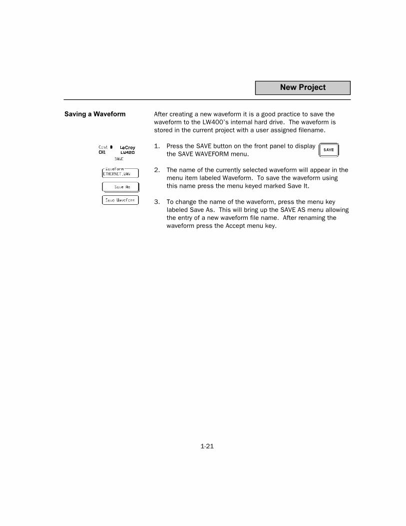
WAVEFORM SELECTION

Figure 3.1 Result of Pushing Select Wave

3-3

GENERAL Selecting a waveform generally implies choosing the desired wave-form to display or playback from a list of options. It may meanselecting a waveform for editing with live feature manipulation byediting one of the channels while it is active. It could also meanediting a waveform in the scratch pad memory so the results of theedit can be viewed without affecting the current state of the output.An additional function is the creation of completely new waveforms.Pushing the button labeled SELECT WAVE near the upper right sideof the AWG rotary control knob causes the AWG to enter a menufrom which these various options can be exercised.

Help! Where is my waveform? (Changing Projects)

If the desired waveform does not seem to be available, it ispossible that it is stored in a different PROJECT than the onecurrently active. This may be remedied by pushing the buttonlabeled PROJECT on the left of the floppy disk drive and opening the correct project. See the section on Project Structure for a moredetailed description of projects and waveform management.

Channel 1/Channel 2 In the box labeled channel 1 or channel 2 there are two choices:Wave/Seq and Waveform*. The former is a toggle switch thatchooses whether or not the output of the selected channel is to bea simple waveform or a sequence of waveforms . See the sectionon Sequence Waveforms for a detailed explanation.

*NOTE: For this discussion it is assumed that the toggle switchhas been set to WAVE.

Select Wave

Table 3.1 Summary of Select Wave menu

Channel 1 Select Waveform or Sequence for Channel 1Channel 2 Select Waveform or Sequence for Channel 2Scratch Pad Select Waveform or Sequence for the Scratch padNew Select a New WaveReference Select A Reference Wave

3-4

The second choice is Waveform. Pushing the associated greysoftkey will cause the Rotary Knob symbol to attach to the wave-form select function. Turning the rotary knob will scroll through thelist of available waveforms. Alternately pushing the associatedgrey softkey again will cause the AWG to display the list of avail-able waveform options on the left side of the screen. Theassociated softkey can be pushed to select the desired waveform.As described previously, if the waveform desired is not in the list,perhaps it is stored in a different project.

Notice that after selecting a waveform for channel 1 or 2, the corre-sponding waveform is now displayed on the screen of the AWG.This waveform is now appearing at the output of the BNC connec-tors as described above provided the output is enabled.

Figure 3.2 Selecting the Wave from a list

Select Wave

3-5

Scratch Pad The Scratch Pad has the same selection options as Channel 1 andChannel 2; however, it has a different functionality. The scratchpad is not directly associated with an output channel. It is, as thename implies, a place to experiment with different waveformoptions before they are committed to an output. Waveforms canbe edited in the scratch pad memory without affecting the state ofthe output of the AWG.

New This is the starting point for creation and naming of a totally newwaveform. Pushing the softkey labeled new activates a sub menupermitting selection of a new channel 1 wave, a new channel 2wave or a new scratch pad wave as a new wave. Selecting one ofthese three options now causes the system to jump to its alphanu-meric entry menu and permits the user to assign a unique name tothis new waveform.

Note that alphanumeric entries may also be made via an IBMPC/AT compatible keyboard connected to the Auxilliary Controlconnector on the rear panel of the LW400. Entries from thekeyboard are limited to upper case letters and numbers. The back-space key may be used to delete text.

Select Wave

Reference

Selecting the Reference Often it is desirable to see a reference wave. For example, it maybe desirable to edit a waveform while viewing the original version ofthe waveform as it is being edited. The reference wave providesthis ability. In the accompanying figure, a reference wave (bottomtrace) is shown simultaneously as the WaveStation user preparesto Edit the active Waveform file (top trace).

Selecting Reference from the SELECT WAVE menu causes theWaveStation to enter a submenu from which it is possible tochoose the reference wave. The choices are the same as for thechannel 1 or channel 2 wave. There is an additional selection toShow Reference. Answering yes permits the reference to beviewed.

3-6

Reference

Figure 3.3 Viewing the Reference

3-7

Display

Figure 3.4 Setting up the display

Splitting the Grid To have two grids as in the figure, it is necessary to enter thedisplay menu. Push 2nd followed by DISPLAY and under Typeselect Dual Grid and push MENU RETURN. For further details seethe following section on DISPLAY.

Display The Display menu is used to setup the type of display, the gridstyle, and the display intensities. Press the red 2ND button andthen DISPLAY ( the alternate function of the ZOOM button). TheDISPLAY menu, shown in the adjacent figure, will appear.

3-8

Display

Type The four display types available are Single, Dual, Single and X-Y,and X-Y. Press the Type softkey to enable selecting the displaytype using the rotary knob. Pressing the softkey a second time willshow all the choices along with individual softkeys for selection.

With Single grid, the selected waveform, or the selected waveformand the reference waveform can be displayed within the same grid.

The Dual grid splits the display into two grids. The selected wave-form is displayed within the top grid. The reference waveform, ifenabled by Show Reference switch in the REFERENCE menu, isdisplayed in the lower grid.

The Single and X-Y grid combines an X-Y display and a singledisplay grid. The Reference waveform is plotted as the Y (ordinate)axis, while the Selected Waveform is plotted along the X (abscissa)axis. This arrangement permits waveform phase relationships tobe investigated as shown in the accompanying figure.

Similarly, the X-Y grid provides a full screen view of the referencewaveform plotted against the selected waveform.

Figure 3.5 X-Y Single Display

3-9

Display

Grid Style Full, Border, or Cross-Hair grids can be selected by pressing theGrid Style softkey. The Full grid includes graticule lines at eachmajor division in the 8 by 10 division display. The Border styleeliminates all the grid lines except for an outer border. The Cross-Hair grid, as the name implies, consists of a set of perpendicularaxes marked with major and minor division increments

Intensity The Intensity menu field is used to set the displayed intensity ofthe waveforms and annotation. When selected, it is adjustableover a range of 1% to 100% using the rotary knob or by numericentry from the keypad. Likewise, the Grid Intensity allows the userto adjust the brightness of the grid lines independently of the wave-form traces.

3-10

Zoom

Figure 3.6 The Zoom Trace Menu

Zoom Pushing the operation key labeled ZOOM on the left of the rotarycontrol knob activates the menu that permits selection of thedisplayed time and amplitude scale factors (zoom factor). TheZOOM controls only affect the display of the waveform. The timebase and amplitude settings of the waveform are not affected bythese settings. There are two major selection fields in thissubmenu. They are Horizontal and Vertical. Each section has twoadditional selections: the value at the center and the appropriatescaling in time or volts per division. Pushing the appropriate greymenu button causes the rotary control to attach to the functionselected. The rotary control is now used to change the value of theselected function. Whenever the rotary control is used to change anumerical value, the resolution of the digit being controlled can bechanged by using the left and right digit button located above therotary control.

3-11

Zoom

When a selected numerical quantity is lowered or raised until eitherthe low or high limit is reached, an error message is printed on thescreen of the AWG. This error message states for example,Cannot decrement this digit meaning that either incrementing ordecrementing the selected digit will exceed the extreme limit forthe field.

Display All Display All causes the entire waveform to appear on the screen. Ithas the effect of undoing any expansions that have previously beeninvoked both in time and in amplitude. This will effect the displayonly, and not the current waveform or output.

Zoom to Cursor Zoom to Cursor will cause the region of the waveform between thetime cursors to expand and fill the screen between the 10% to 90%horizontal grid line.

Zoom Previous Toggles between the current and previous ZOOM setting.

3-12

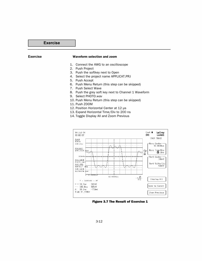
Exercise Waveform selection and zoom

1. Connect the AWG to an oscilloscope2. Push Project3. Push the softkey next to Open4. Select the project name APPLICAT.PRJ5. Push Accept6. Push Menu Return (this step can be skipped)7. Push Select Wave8. Push the grey soft key next to Channel 1 Waveform9. Select PHOTO.wav10. Push Menu Return (this step can be skipped)11. Push ZOOM12. Position Horizontal Center at 12 µs13. Expand Horizontal Time/Div to 200 ns14. Toggle Display All and Zoom Previous

Figure 3.7 The Result of Exercise 1

Exercise

4-1

LIVE WAVEFORM MANIPULATIONS4

Cursor Manipulations Live waveform manipulation means selecting some feature of awaveform and changing it while the output is also modified. Thischange does not occur in real time: there is some delay betweenfeature manipulation in the AWG and a change in the state of theoutput which is proportional to the size of the area affected.

The first step in live waveform manipulation is to use the timecursors to select a region of interest in the waveform. This mayalso involve using the Zoom controls discussed previously. Byusing Zoom to expand the waveform a detailed examination andselection of waveform elements can be accomplished. This willhelp assure accurate results of a waveform manipulation of aspecific feature.

Time Cursors Pressing the Operation key labeled TIME CURSOR next to therotary control knob activates the menu depicted in figure 4.1 andsummarized in table 4.1 below. The time cursors consist of twovertical bars that can be positioned on either side of a waveformfeature in order to manipulate extract or delete that feature when

Figure 4.1 Time Cursor Menu

4-2

Time Cursor

editing. (See editing waveforms in section 6). The time cursorsmay not cross one another. Time cursors are used in all editing,functions and measurements. Measurements and Cut editingoperations use both cursors while Paste and other Insert opera-tions use the left Cursor.

Help ! Where are the Cursors? When the cursors are first turned on, it is possible that they are not

visible on screen. Try pushing the softkey labeled Cursors to Gridimmediately. The reason the cursors may not be seen initially isthey are located on a portion of the waveform that is outside thefield of view. This can occur if, for example, the waveform hasbeen previously expanded and recentered using the ZOOMcontrols. Notice it is possible to manipulate the cursors indepen-dent of viewing them: the AWG knows where the cursors are even ifthey are not being displayed. Similarly Cursors To End may movethe cursors off the screen and outside the field of view if thepresent state of the expansion is such that the end of the wave-form is outside the field of view.

Another reason the cursors may not be visible is because they arelocated directly over a display gradicule line. Turning the rotarycontrol knob will bring the selected cursor into view.

Table 4.1 Summary of Time Cursor Operations

Time Cursor On/Off This toggle switch selection turns the timer cursors on or offTrack On/Off With track set to On, the right cursor moves with left cursor at a fixed

time difference (DELTA) when the left cursor is selected and moved.Measure On/Off This toggle switch turns the measurements on or off Time Left Select this field to move the Time Left Cursor Time Right Select this field to move the Time Right Cursor Delta Change the delta between the cursorsSelect All Position the cursors to surround the entire waveformCursors To Grid Move the cursors onto the grid (see discussion below)Cursors To End Move both cursors to the right end of the waveform

4-3

Measure When the measurements are on they will be displayed in thebottom center of the screen (below the grid). Six measurementswill be made: min, max, rise time, fall time, period (PER) and width(WIDP). Min will be the minimum amplitude between the Time Leftand Time Right cursors. Max will be the maximum amplitudebetween the Time Left and Time Right cursors. Rise time and Falltime will be the first respective qualifying edge after the Time Leftcursor and are 10% to 90%. Period will be the time between twoodd numbered 50% crossings beginning with the 1st crossingsafter the left cursor. WIDP is the time between adjacent 50%crossings for the first positive pulse between the cursors. See Appendix A for more detail.

Voltage Cursors Pressing the menu selection key labeled Voltage Cursors next tothe rotary control knob activates the submenu seen in figure 4.2and summarized in the table below. The voltage cursors consist of two horizontal bars that can be positioned up or down along thewaveform. The voltage cursors may not cross one another. Thesecursors are used for making measurements on waveforms.

Voltage Cursor

Fig. 4.2 Voltage Cursor Menu

voltage cursors

4-4

Live Manipulations Many Time Editing operations are performed as quickly as possiblein response to user input. The LW400 attempts to compute thedesired waveform immediately when the state is changed. If therequested state is changed again before the computation iscompleted, the partially completed computation is discarded and anew attempt to compute the desired waveform is begun.

If the waveform being edited is the active waveform for one of thechannels, then it is automatically updated when the new waveformis computed. The output holds a data point from the previouswaveform while the new playback image is being loaded. The play-back of the new image begins at its first value.

Voltage Cursor

Table 4.2 Summary of Voltage Cursor Operations

Volt Cursor On/Off This toggle turns the voltage cursors on or offTrack On/Off With Track set to On, the voltage cursors move together at a

fixed voltage difference (DELTA) when the top cursor is moved.Volt Top Select this field to move the top voltage cursorVolt Bottom Select this field to move the bottom voltage cursorDelta With track On, this is the voltage difference between the top

and bottom cursorsCursors To Grid Position the cursors on the grid from their current location

4-5

Time Edit Press the Time button in the Edit group to get the menu of figure4.3. From this menu the duration of part or all of a waveform canbe rescaled, or shifted (delayed) in time. Changing the duration of aregion always expands or compresses it horizontally: verticalscaling is not affected.

Duration Stretches and compresses the waveform between the cursors hori-zontally, in time. The left cursor remains in a fixed position and theright cursor moves to the left or right depending on the direction inwhich the rotary knob is turned. A number for duration can also beentered using the numeric keypad. As the right cursor slides inresponse to the input, the amplitude value at the right cursorremains fixed. The method of insertion depends on the selectionof mode described below.

Note that using duration provides a quick way to rescale an entire waveform. Using the time cursors, select all, then changeduration.

Time Edit

Fig 4.3 The Edit Time Menu

4-6

Time Edit

Mode In Overwrite Mode the length of the waveform doesnt change as aregion is rescaled: as the region expands, data to the right of theregion is overwritten; as the region shrinks, amplitude of the right-most point is replicated to keep the waveform length constant. InInsert Mode the waveform size increases and decreases as theregion increases and decreases.

Move Feature Slides the region, or feature, between the cursors over the wave-form. As the region slides, the waveform values are linearlysuperimposed on each other. The precision with which a featurecan be placed is 100 psec.

Capture Feature As a waveform feature is moved the linear addition causes newfeatures to be formed. That is for example, a pulse sliding overanother pulse and adding to it will cause a new pulse that is the sum of the two. If it is now desired to capture this newfeature and move it, then press Capture Feature. The memory willnow lose the old feature and begin to slide the new feature inits place.

Delay Takes the entire waveform starting with the left cursor and slides itto the right or left by an amount equal to the value in the Delayfield. This is done with a maximum precision, or resolution of 100 psec.

4-7

Time Edit

Fig. 4.4 Moving the feature in PHOTO.WAV

1. Refer back to Exercise 1 for WaveformSelection & Zoom

2. Press Time Cursor3. Position the Time Left and Time Right

Cursor around a small section of thewaveform

4. Press Time in the Edit section5. Select Move Feature and turn the Rotary

Knob. Observe the effort on the oscilloscope.

6. Push UNDO on the keypad and answer ok7. Select Duration and turn the Rotary

Knob. Observe the effort on the oscilloscope.

8. Repeat step 69. Select Delay and change it with the

Rotary Knob. Again, observe the effort onthe oscilloscope.

10. Repeat step 6 to Undo your changes

Live Waveform Manipulation

4-8

Amplitude Edit Press the Amplitude button in the Edit group to get the menu offigure 4.4. From this menu the amplitude of all or selectedportions of the active waveform can be manipulated live.

Amplitude Edit

Figure 4.4 The Edit Amplitude Menu

Amplitude Sets the peak-to-peak amplitude of the waveform between the two cursorswith respect to the baseline.* The baseline is the line drawn between thetwo cursors

Median Sets the median voltage of the displayed waveform between the time cursorsMax Voltage Sets the maximum voltage of the displayed waveform between the time

cursorsMin Voltage Sets the minimum voltage of the displayed waveform between the time

cursors

Table 4.3 Summary of the Edit Amplitude menu

*Note: The baseline is the reference line shown on the display,connecting the points where two cursors intersect the waveform.Ifthe baseline termination points are not of equal amplitude thebaseline will be sloped.

4-9

Live Waveform Inversion Waveform inversion (i.e. multiply by -1) is available as an amplitudeedit function. As in all of the edit functions, the portion of the wave-form between the time cursors is affected by the invert operation. Itis possible to invert all or part of the waveform.

In the example shown in the top trace of the accompanying figure,the portion of the waveform between the time cursors has beeninverted. The lower trace is the reference waveform, showing theoriginal waveform. Note that the signal is inverted about the editbaseline (the line connecting the points on the waveform inter-sected by the time cursors). In this example the baseline is set tobe 0 Volts.

Amplitude Edit

Figure 4.5 The Invert softkey in the Amplitude Edit menu

5-1

INSERT WAVE5

Edit Insert Wave Menu There are many different sources of waveforms available to the

user of the LW400 Series Arbitrary Waveform Generator.Waveform files may be transferred directly from a variety of oscillo-scopes without the need for an intermediate computer. They mayalso be transferred from other LeCroy arbitrary function generators.Especially important to current users of LeCroy AFGs is the abilityto transfer EasyWave files to the LW400. If a function can bedescribed with an equation, then the built in equation editor shouldmake entry relatively painless. Waveform files may be input in anASCII format from any source. In addition, a variety of standardfunctions are available as a starting point for waveform creation.

All of these functions can be accessed from Insert Wave, assummarized in table 5.1.

Fig 5.1 The Edit Wave Menu

5-2

Insert from DSO

From Scope DSO Type This is the type of digital oscilloscope that the waveform will bedownloaded from. There are many available choices includingoscilloscopes from LeCroy, Hewlett Packard, and Tektronix. Otheroscilloscopes may be added by importing an appropriate digitaloscilloscope configuration (DSO) file using the Import function inthe Project menu.

GPIB Address This command does not set the address of the scope or the AWG.It tells the AWG what address the DSO is already set for.

Table 5.2 Summary of Get From Scope menu options

DSO Type Selects from the list of available scopesTrace Source Selects which (DSO) Trace to get the waveform fromDSO GPIB Address Selects the scopes GPIB address (see below)Preserve Time/Pts Preserve time resamples the data keeping the waveform duration

constant. Preserve points reproduce each sample acquired fromthe DSO but at the LW400s clock period

Request Control yes/no Set to yes if LW400 is installed in a system with another GPIB controller on the bus.

Execute Transfers the waveform from the DSO to the AWG

Table 5.1 Summary of Sources from which Waves may be inserted

From Scope Waveforms can be inserted from a variety of scopes (Section 5.1)Standard Waves There are a variety of standard waves (Section 5.2)Equations The equation editor is described in Section 5.4Other Waves Insert other waveforms from current project

5-3

Insert from DSO

Preserve Time/Pts This choice allows the operator to select between preserving theshape in absolute time of a waveform that is being transferred orto preserve the number of points. For example, suppose a DSOhas sampled a waveform at 200 Megasamples/second and theWaveStation is running at a clock speed of 400 Megapoints persecond. Preserving time means the waveform coming from thescope is resampled to match the faster clock speed of the AWGand thus will have twice as many points.

Preserving points, on the other hand, means the reconstructedwaveform will have twice the frequency content of the original wave-form. This is because the reconstructed waveform will have thesame number of points however; since the AWG is going twice asfast as the scope, the new points will be spaced closer together.

The choice to preserve the number of points has the potential tochange the frequency content of a signal unless the WaveStationclock is adjusted accordingly but it preserves the exact shape ofthe waveform.

Figure 5.2 Insert From Scope

5-4

Insert from Standard Waves

Standard Waves A library of standard waves is available. Figure 5.2 shows themenu selections available in the standard waves menu. The tablesbelow summarize the characteristics of these waves.

Sine

Variable Range Resolution Default Value

Amplitude (peak-to-peak) 0 mV - 10 V 1mV 1 VoltOffset @ zero phase +5 V to -5 V 1 mV 0 VoltsFrequency 1 Hz to 100 MHz 1 ppm 10 MHzCycles 0.01 to 65 k 1 or 10 10 cyclesStart Phase (see note below) 0 to 360 .05 degree 0 degree

Figure 5.3 Standard Wave Selection

5-5


Square

Ramp

Triangle


Amplitude (peak-to-peak) 0 mV - 10 V 1mV 1 VoltOffset @ zero phase +5 V to -5 V 1 mV 0 VoltsFrequency 1 Hz to 25 MHz 1 ppm 10 MHzCycles 0.01 to 65 k 1 or 10 10 cyclesStart Position 0 to 100% 1 m % 0.0 %Invert on/off off


Amplitude (peak-to-peak) 0 mV - 10 V 1mV 1 VoltOffset @ zero phase +5 V to -5 V 1 mV 0 VoltsFrequency 1 Hz to 25 MHz 1 ppm 10 MHzCycles 0.01 to 65 k 1 or 10 10 cyclesStart Phase (see note below) 0 to 360 .05 degree 0 degree


Amplitude (peak-to-peak) 0 mV - 10 V 1mV 1 VoltBase +5 V to -5 V 1 mV 0 VoltsFrequency 1 Hz to 50 MHz 1 ppm 10 MHzCycles 0.01 to 65 k 1 or 10 10 cycles1Time Delay 0 ns to mem. length 1 ns 0 ns1Edge Time (risetime and falltime) 5 nsec to 500 ns 1 ns 5 ns

1. This range is given for the 400 MS/s clock rate. This range is scaled with the clock rate.

5-6


DC


Level + - 5V 1mV 1VoltDuration 10 ns to mem length 1ns 10 usec

1. This range is given for the 400 MS/s clock rate. This range is scaled with the clock rate.2. Maximum period and width are related to the length of waveform memory. Numbers quoted are for 1 Mbyte memory.

Pulse


Amplitude (peak-to-peak) 0 mV - 10 V 1mV 1 VoltBase +5 V to -5 V 1 mV 0 Volts1, 2Period 10 ns - 2.5 ms 1 ppm 10 MHzCycles 0.01 to 65 k 1 or 10 10 cycles1, 2Width 0 to 2.5 ms 1 ns 5 nsTime Delay 0 to memory length 1 ns 0 ns1Edge Time (risetime and falltime) 5 nsec to 500 ns 1 ns 5 ns

5-7

Edit Equation

Equations Any waveform that can be described by an equation using the 11basic waveform functions, can be entered via the equation editor.This includes simple everyday functions like sine waves andpulses, and extends to very complex mathematical expressions.The equation editor provides an environment for entering, editingand calculating mathematical functions.

This section of the manual describes the equation editor and theassociated functions and arguments.

Waveform Equation Notebook A separate publication called the Waveform Equation Notebook

gives examples of many functions and their associated equations.The Waveform Equation Notebook is included with this manualsection.

5-8

Edit Equation

Select LineThis field allows a user to select one of the 16 lines in the equa-tion. This is the equation line that is calculated. A valid linenumber can be entered using the numeric key pad or the rotaryknob can be used to move the line cursor. The cursor will not wraparound from line 16 to line 1, it will stop at the extremes.

Figure 5.3 Edit Equations

Table 5.3 Summary of Edit Equation Options

Duration This is the duration of the waveform that is calculatedEdit Equation Line Enter an equation on the selected lineNew Start or name an equationOpen Get an already existing equationSave Save an equationCalculate Calculate the equation in the selected line and produce a waveform

5-9

Edit Equation

Edit Eqn Line On entering this menu the select line bar will go away and the textcursor will appear at the beginning of the selected line. When theFunctions, Operators, Variables, or Arguments field is pressed,the lists are expanded, allowing the user to choose a list item.When the list item is selected (by pressing the softkey next to theitem) it will be inserted into the equation. Constants can be placedinto the equation by using the numeric key pad. No attempt will bemade to make sure that the equation is syntactically correct, it issolely up to the user. If an incorrect equation is calculated, theuser will be told there is an error in the equation. References canbe made to include other lines of the equation sheet by definingvariables. The entire equation will be expanded (internally) but theexpanded version must not exceed 1024 characters.

Figure 5.4 The Equation Editor

5-10

Edit Equation

Functions The following functions can be used in equations; AbsoluteValue(ABS), Cosine(COS), Exponent(EXP), Integer Floor (FLOOR),Natural Logarithim(LN), Common Logarithim(LOG), Pulse (PULSE),Sine(SIN), Square Root(SQRT), Unit Step(STEP), Tangent(TAN).Since all these functions require a ( ) after the function name, itwill automatically be inserted and the cursor will be placed betweenthe parentheses.

Operators The available operators are; Add(+), subtract(), multiply (*),divide( /), group ( ), comma (,) and raise to a power( ^).

Variables You can define a variable in the form of X# = <any valid equationincluding constants>, where # ranges from 1 to 16. These vari-ables can be used in the middle of another equation, e.g. X1 + X2.

Arguments Includes: 2*PI*T, T, PI, NOISE and GNOISE. NOISE returns apseudorandom series of values with uniform amplitude distribution.GNOISE returns a pseudorandom sequence with Gaussian distributedamplitude values. Note: T = 0 at the left cursor.

Figure 5.5 The Functions List

5-11

Edit Equation

Move Cursor This field has the rotary knob and numeric keypad attached to it.The text cursor is moved by turning the knob or entering thenumeric position desired.

Backspace Backspace will delete the character to the left of the cursor.

Accept Enters the selected line and returns the user to the main EQUA-TION menu and the highlight bar will be restored.

Note: exiting this menu without pressing Accept causes no action to be taken.

New This field contains the name for a new equation. The number keypad and the keyboard (if present) will be active. It is 14 charactersin length and can contain spaces. Entering and accepting a newequation name will close the contents of the equation editor.

Open A list of available equations to open.

Save On entry to the menu this field contains the name of the openequation. If a new name is entered in the Save As menu (seebelow) then this field contains that name.

Save As This menu acquires the name under which to save the currentequation.

Save It Saves the equation. Note: if the project that the equation belongsto is write protected then the user will be told its a write protectedproject and abort the save operation. If a new name was enteredfor the equation (Save As) then a new equation is created from thecurrent equation. The old equation is closed (no prompt is given ifthe equation has changed) and the new equation is opened.

Calculate Calculates the data points of the selected equation and inserts itinto the waveform in the INSERT mode. This is the only way tocalculate and insert the equation. Exiting this menu withoutpressing Calculate causes no action to be taken.

5-12

Edit Equations

Waveform Equation Note book

Creating Waveforms From Equations Equations offer the most precise method of creating a waveform in

the LeCroy WaveStation, LW400 Series Arbitrary WaveformGenerator. This notebook is intended to provide examples ofcommonly used waveforms and the equations which describethem. It also provides examples of waveform creation techniqueswhich can be applied more generally.

LW400 Equation Functions And Operators The WaveStation equation editor includes 11 mathematical func-

tions and 9 operators, which are described briefly below.

Functions

ABS ( ) Absolute value, calculates the absolute value, unipolar magnitude, of a function or argument

COS ( ) Cosine, calculates the cosine of the argument

EXP ( ) Exponential, calculates an exponential, using the base of natural logarithms, e, raised to the power specified in the argument

FLOOR ( ) Floor, calculates the integer floor of a function

LN ( ) Natural Logarithm, calculates the natural logarithm, base e, of the argument or function

LOG ( ) Common Logarithm, calculates the common logarithm, base10, of the argument or function

PULSE ( ) Pulse, creates a pulse using edge locations, or functions, specified in the argument

SIN ( ) Sine, calculates the sine of the argument

SQRT ( ) Square root, calculates the square root of the argument or function

STEP ( ) Step Function, creates a unit step at the location specified by the argument or function

TAN ( ) Tangent, calculates the tangent of the argument

5-13

Operators

+ Addition

- Subtraction

* Multiplication

/ Division

( Mathematical grouping

) Mathematical grouping

, comma separator for arguments

= equality

^ Raise to a power (exponentiation)

Variables The variables X1 - X16 can be used to label the contents of anyline on the equation editor. The variable can then be used toreplace the contents in another equation.

Example: X1 = SIN(2*PI*10E6*T)X2 = (1+ 0.75 * COS(2*PI*1E3*T))X1*X2

The product X1*X2 will be computed as follows:

X1*X2 = SIN(2*PI*10E6*T ) * (1+ 0.75 * COS(2*PI*1E3*T))

Arguments There are five functional arguments available for use in equations:

2*PI*T Phase variable for trigonometric functions, in radian seconds

T Time variable, in secondsPI Numerical Constant 3.14159265358979 NOISE Uniformly distributed random numbers 0-1,

mean = 0.5, standard deviation = 0.288GNOISE Gaussian distributed random numbers 0-1,

mean = 0.5, standard deviation = 0.1667

Edit Equations

5-14

Constants Numerical constants can be entered from the keypad on the frontpanel. Use the units multiplier entry keys, p(pico, 1E-12), n (nano,1E-9), µ or u (micro, 1E-6), m (milli, 1E-3), ENTER (units, 1), k (kilo,1E3), M (Mega, 1E6) to specify the correct multiplier. For example7.5 M = 7.5 E6 and 2n = 2 E-9

Wave Math Equations are used in the creation of waveforms from an analyticaldescription. Wave Math is a waveform array processor which oper-ates on entire waveforms, regardless of their source. Theoperations available in wave math include:

SmoothingWaveform AdditionWaveform SubtractionWaveform MultiplicationWaveform DivisionIntegrationDifferentiationConvolution

These operations are available in addition to equation entry but areunique in that they operate on entire waveform. Wave Math opera-tions are covered in a separate section.

Using The Equation Notebook In the following examples each waveform type includes a general

equation showing the functions, arguments, and variables required.User entered constants are described in general terms. Theaccompanying waveform includes a specific numerical example. Itprovides the actual equation used to create the waveform shown.

Edit Equations

5-15

Waveform General Equation LW400 Example

1. Unit Step STEP (T-T° )

T° - Edge location in seconds

2. Time Reversed STEP (T° -T)Step(Step Down) T° - Edge location

in seconds

3. Unit Pulse PULSE (T1,T2) or STEP (T-T1) - STEP (T-T2)

T1 - Time of leading edge in seconds

T2 - Time of trailing edge in seconds

Edit Equations

5-16


4. Pulse Train STEP (SIN (2*PI*T*FS )) FS - Pulse frequency in Hertz

Note: The LW400 function STEP ( ) accepts other func-tions, f(t), as an argument:

STEP ( f(T)>0) = 1STEP (f(T) <0) = 0

5. Tri-level Pulse PULSE (T1,T2) - PULSE (T3,T4)

T1 ,T3 - Time of leading edges in seconds

T2 , T4 -Time of trailing edges in seconds

6. Ramp A * T

A - Slope of ramp (DV/DT)

Edit Equations

5-17


7. Delayed Ramp A * ( T-TD ) * STEP (T-TD )

A - Slope of ramp (DV/DT)TD - Time delay, seconds

8. Truncated Ramp A * (T-TD ) * PULSE ( TD, TL )

A - Slope of ramp (DV/DT)TD - Time delay, secondsTL - Length of ramp, seconds

9. Negative Ramp - A * ( T-TD ) * PULSE (Truncated) ( TD, TL )

A - Slope of ramp (DV/DT)TD - Time delay, secondsTL - Length of ramp, seconds

Equation Notebook

5-18


10. Trapezoidal X1=-A * (T-T1)* STEP (T-T1)Pulse X2= A * (T-T2)* STEP (T-T2)(with adjustable X3= A * (T-T3)* STEP (T-T3)rise and fall X4=-A * (T-T4)* STEP (T-T4)times)

A - Edge slope (DV/DT)T1 - Leading edge start time T2 - Leading edge end timeT3 - Trailing edge start timeT4 - Trailing edge end timeall times in seconds

11. Sine V * SIN(2*PI*T*FS )

FS - Signal frequency, HertzV - Signal amplitude, V P-P

12. Gated Sine V* SIN(2*PI*T*FS )*STEP (T-TG )

FS - Signal frequency, HertzV - Signal amplitude, V P-PT° - Gate start time, seconds

Equation Notebook

5-19


13. Sine Burst V*SIN(2*PI*T*FS)* PULSE(TS,TE )

V- Signal amplitude, V P-PFS - Signal frequency, HertzTS - Burst start time TE - Burst end timeall times in seconds

14. Decaying EXP( -T / TC )Exponential

TC - Time constant, seconds

15. Delayed EXP (-( T-TD ) /T C )*Exponential STEP(T-TD ) Decay

TC - Time constant, secondsTD - Time delay, seconds

Edit Equation

5-20


16. Rising 1- EXP (-T/TC)Exponential

TC - Time constant, seconds

17. Delayed 1-EXP(-(T-TD)/TC)*Rising STEP(T-TD)Exponential

TC - Time constant, secondsTD - Time delay, seconds

18. Exponential X1=(1-EXP(-(T-T1)/T2))* Pulse With PULSE(T1, T3)Different X2=(EXP(-(T-T3)/T4)* Rise And Fall STEP(T-(T3))Constants X1+X2

T1 - Delay of rising edgeT2 - Time constant of riseT3 - Delay of falling edgeT4 - Time constant of fall³T - Sample period

Edit Equation

accused

5-21


19. Exponentially V*EXP(-T/TC) * Damped Sine SIN(2*PI*T*FS)With Gain

FS - Signal frequency, HertzTC - Time constant, secondsV- Signal amplitude, V P-P

20. Gaussian EXP( -(1/2)*(( T-TM )/Ts)^2)Pulse

TM - Time location of center or mean of Gaussian pulseTs - Half width of Gaussian point corresponds to standard deviation, s .

21. Amplitude X1 = SIN(2*PI*T*FC)Modulation X2 = (1+ K * f (T))

X1*X2

f (T)- Modulating waveform, a function of T: e.g SIN(2*PI*T*FM)FC - Carrier frequency, HertzFM - Modulation frequency, HertzK - Modulation index, 0<K<1

Edit Equation

5-22


22. Sine (A*T) * SIN(2*PI*T*FS ) AmplitudeSweep A - Slope of ramp

FS - Signal frequency, Hertz

23. Frequency SIN(( 2*PI*T*FC+(FD/FM)* Modulation COS( 2*PI*T*FM )

FC - Carrier Frequency, HertzFD - Frequency Deviation, Hertz FM - Modulation Frequency

Note: For frequency modulation the phase argumentof the SIN function includes the integral, ∫ f(t), of thedesired modulation function, f(t): e.g. for sinusoidalFM f(t) = SIN(2*PI*FM*T) the phase argumentcontains f(t)=COS(2*PI*FM*T)/(2*PI*FM)

24. Linear SIN(PI*(2*T*FS+Frequency ((FE-FS)/TS)*T^2))Sweep

FS - Start frequency, HertzFE - End frequency, HertzTS - Sweep duration, seconds

Edit Equation

5-23


25. Logarithmic X1 = LN (FE/FS)/TS

Frequency SIN(2*PI*(( FS/ X1)*Sweep EXP( X1*T )-1)))

FS - Start frequency, HertzFE - End frequency, HertzTS - Sweep duration, seconds

26. Phase SIN(2*PI*T*FC+K * Modulation SIN( 2*PI*T*FM))

FC - Carrier frequency, HertzFM - Modulation frequencyK - Peak phase excursion, radians

27. Pulse Width X1=SIN(2*PI*T*FC+K*Modulation COS(2*PI*T*FM)

X2=SIN(2*PI*T*FC+K*SIN(2*PI*T*FM)STEP (X1) * STEP (X2)

FC - Pulse frequency, HertzFM - Modulation frequencyK - Peak phase excursion, radians

Edit Equation

5-24


28. Pulse A*T*STEP(SIN(2*PI*T*FC)Amplitude Modulation A - Slope of ramp,

Volts/secondFC - Pulse frequency, Hertz

29. Lorentz Pulse 1/(1+(( T-TD ) / TW ) ^ 2)

TD - Time delay, secondsTW- Half width @ 50% amplitude, seconds

30. Full Wave ABS (SIN (2*PI*T*FS))Rectified Sine


Edit Equation

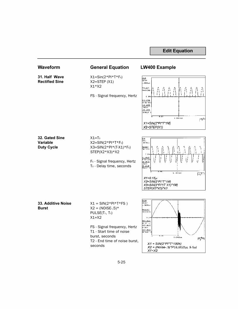
5-25


31. Half Wave X1=Sin(2*PI*T*FS)Rectified Sine X2=STEP (X1)

X1*X2


32. Gated Sine X1=TD

Variable X2=SIN(2*PI*T*FS)Duty Cycle X3=SIN(2*PI*(T-X1)*FS)

STEP(X2*X3)*X2

FS - Signal frequency, HertzTD - Delay time, seconds

33. Additive Noise X1 = SIN(2*PI*T*FS )Burst X2 = (NOISE-.5)*

PULSE(T1, T2)X1+X2

FS - Signal frequency, HertzT1 - Start time of noise burst, secondsT2 - End time of noise burst, seconds

Edit Equation

5-26

Other Waves

Other Waves

Waveform A list of available waveforms to insert. These are the waveformsthat are stored in the open project. For a discussion of the projectstructure, see Project Section 10 in this manual.

Accept Inserts the waveform in the field Waveform starting at the leftcursor.

Returns to the main INSERT menuNote: exiting this menu without pressing Accept causes no actionto be taken.

6-1

WAVEFORM & EDITING6

Getting Started Editing operations include the creation and modification of wave-forms. The controls within the EDIT section of the front panelprovide a complete set of tools for waveform creation as well ascut and paste editing. In this section we will look at the EDITfunctions.

Clearing The Display The easiest way to clear one of the AWGs editors is to select anew waveform. The process was discussed in the tutorial insection 2.

Exercise 6.1 1. Push SELECT WAVE2. Press the NEW softkey in the SELECT WAVE menu3. Push NEW CH1 WAVE in the NEW menu.4. Enter the desired waveform name, for instance New, then

press the Accept softkey.

Figure 6.1 Result of Exercise 1

6-2

The Edit Menu Pressing the EDIT button in the EDIT group on the front panel ofthe LW400 causes the EDIT menu to be displayed:

Edit Menu

Figure 6.2

The Edit Menu

Table 6.1 The Edit Menu Functions

Softkey Label Function

Properties Selects editor options: insert or over-write and insert before or after thecursor. Also used to select waveoptions: oversampling yes/no andcontinuous or single waves.

Cut Selects Delete, Copy, or Extract opera-tions to remove or copy a selectedsection of a waveform to the cut buffer.

Paste Selects Paste operations to copy thecontents of the cut buffer to the wave-form at the selected insertion point.

Insert Wave Inserts a waveform segment from aDSO, equation editor, standard func-tion, or another waveform into thecurrent waveform at the selected inser-tion point.

Digital Edit Selects digital edit menu. This menuselection only appears if theLW09/LW09A digital option is installed.

Marker Selects the Marker edit menu used tosetup the timing marker(s) associatedwith the waveform.

Edit Sequence Selects the sequence editor for creatinga composite waveforms and group

6-3

Edit Properties

Figure 6.3

PropertiesMenu

Pressing the EDIT button in the EDIT group on the front panel ofthe WaveStation displays the EDIT menu. Select properties tochoose the editing insertion technique to be used.

Editor Options

Ins/Ovr Overwrite inserts the new section starting at theleft time cursor and overwrites, or replaces,existing sections without increasing the overallduration of the waveform, however it may increasethe total duration. It acts the same as the similarfunction in a word processor.

With Insert the new waveform section is inserted atthe left cursor and moves all the data to the right ofthe cursor (not including the point under the leftcursor) by the length of the inserted section. Onceagain, this is similar to insert in a word processoras it pushes the old data out of the way andchanges the length accordingly.

Insert before or after cursor?This editor option tells the editor what to do withthe cursors after inserting new sections into thewaveform. If Before is selected, then upon inser-tion of the new section into the waveform the leftcursor is moved to the end of the insertedsectionleaving the inserted section before thecursor. If After is selected then the left cursor isnot moved upon insertion of the new section is intothe waveform.

The Properties Menu

6-4

Edit Properties

Wave optionsWaveform options apply to the currently selectedwaveform. These options are saved with the wave-form when the wavefo rm is saved.

Type This is an information field only. It displayswhether the selected waveform is an ANALOGwaveform or a DIGITAL waveform.

Oversample waveIn order for the LW400 to edit a waveform, thewaveform must be oversampled. Many of theediting functions apply signal processing that usesa sinx/x interpolator. The interpolator will createsignificant ringing if the data is not oversampled.If this field is set to Yes then the waveform will bechecked for discontinuities and if found they willbe fixed by passing the discontinuity through a lowpass filter. If No is chosen then the data will notbe checked for discontinuities. The limitation withthis is that no editing operations can be applied tothe waveform until it is oversampled. The advan-tage is oversampling slows the edges by requiringat least two points on every edge. So, by turningoversampling off, faster edges can be achieved.

Waves are Use to select if the WaveStation is to considersthe waveform a single shot waveform or a contin-uous waveform (last point wrapped to the first).Continu-ous waveforms are displayed with theends wrapped in a dimmer shade on the screen.The WaveStation will check for a discontinuitybetween the end and the beginning of the wave-form. This makes the presumption that when theLW400 reaches the end of the waveform it willjump to the beginning and play the first point. Ifthe waveform is only to be played once (singleshot) or, is part of a sequence where wrapping theends might be an incorrect thing to do, singleshould be selected for this field.

6-5

Edit Mode

Creating A Waveform With Insert Wave

The Insert Wave function can be used, as it was in the tutorial, tocreate a distinctive waveform to demonstrate editing operations.Standard Function sine, square wave, and triangle waves wereused to create the waveform shown in figure 6.3.

Figure 6.3 A Waveform Created With Insert Wave

6-6

Cut

Table 6.2 Summary of Cut Functions

Softkey Label Function

Delete Erases the section of the current waveform between the time cursorsand copies it to the cut buffer. The waveform duration is reduced by thecursor time difference.

Copy Copies the section of the waveform between the time cursors to the cutbuffer without removing it from the original waveform.

Extract* Erases the section of the current waveform between the time cursorsand copies it to the cut buffer. The removed waveform section isreplaced by a baseline level.

Baseline Sets the mode for baseline generation either automatic or manual.Automatic baseline is determined by the value at the left, right, or bothcursors as selected by the user in the Attach field. Manual baselineallows user entered values to desribe the end points of the baseline.

Attach Sets the end points of the automatic baseline as the amplitude value ofthe left, right, or both cursors.

Baseline Attach Action

Auto Left Baseline is set at the amplitude value read at the Time Left cursor

Auto Right Baseline is set at the amplitude value read at the Time Right cursor

Auto Both Baseline is drawn connecting the amplitudes at the Time Left cursor andthe Time Right cursor

Man Left/Right Baseline is drawn between the user entered amplitude values specifiedin the Left and Right entry fields. Automatic baseline is determined bythe value at the left, right, or both cursors as selected by the user in theAttach field. Manual baseline allows user entered values to desribe theend points of the baseline.

Cut The Cut functions include Delete, Copy, and Extract which aredescribed in table 6.2 and cut baseline actions in table 6.3.

Table 6.3 Summery of Cut Baseline Settings

6-7

Delete

Figure 6.5 Result of the Delete operation

Figure 6.4 Setup for a CutDelete operation

Delete The following figures show the setup for a Delete operation on thesquare wave section of the waveform. Figure 6.4 shows the place-ment of the time cursors about the section to be deleted. Figure6.5 shows the result of the deletion. Note that the waveform isshortened by the duration of the deleted section. Pressing theUNDO button, located on the front panel, and confirming undo withOK will restore the original waveform.

6-8

Extract

Figure 6.6 The result of an Extract operation

Extract The results of an Extract operation are shown in figure 6.6 for thesame cursor settings. Note that the waveform retains its originalduration and that the extracted section is replaced by a baseline.The baseline, created in Auto-Both mode, connects the amplitudevalue under the time left cursor (-499 mV) to that of the time rightcursor(-500 mV). Alternative baseline settings are outlined in table6.3 shown on page 6-4..

* Extract is useful in editing small features which occur on a basewaveform. For example, adding a glitch to a sine wave.

6-9

Paste

Figure 6.8 Pasting after an Extract operation

Paste Paste copies the contents of the cut buffer into a waveform at aninsertion point marked by the Time Left cursor. The number ofrepetitions of the insertion is users selectable from the PASTEmenu.

The results of the paste operation will change depending onwhether the waveform in the cut buffer came from a Cut/Delete,Copy, or a Cut/Extract operation. Examples are shown in figures6.7 and 6.8.

Figure 6.7 Pasting after a Delete operation

If the cut buffer was filled as a resultof a Copy or Delete operation thenthe waveform is inserted into, oroverwrites, the waveform dependingon the edit mode. If the contents ofthe cut buffer are from an extractoperation, they are added to thewaveform.

7-1

SEQUENCE WAVEFORMS

Introduction to Sequences

The Wavestation includes the capability of generating a waveformsequencecomprised of waveformsand a waveform groupsequencecomprised of sequences. Both types of sequences aidin generating long, complex waveforms. The group sequencemode has the capability of switching from one waveform sequenceto the next in less then 5 ms. Both modes are useful for generatingcertain types of long, complex waveforms while minimimizing theamount of memory.

In sequence modewaveform sections that repeat are made intosegments that are repeated with loopseffectively generating thewaveform using minimal memory. Each waveform and its number ofrepetitions are stored in a sequence list. The wavestation outputsthe waveforms sequentially, the specified number of times.

In group sequence mode, waveform sequences are specified in agroup list for processing. The first sequence in the list is outputuntil an advance command or a jump command is received. Whenadvance is received the next waveform in the list is output. If ajump command is received, the waveform selected by the jumpcommand is output.

7

7-2

Sequence Waveforms

Sequence mode A sequence is the result of concatenating a number of waveformfiles in a specified fashion. Suppose, for example, it is desired togenerate a TV signal. The TV signal is composed of a number ofdifferent elements. There is the equalization pulse followed by thevertical synch pulse followed by more equalization pulses then thebeginning of the color burst and horizontal synch informationfollowed by video information and so on. This signal can be gener-ated from the smaller parts, or segments, by a process calledlinking. In linking, the individual waveform segments areconnected together in the correct order, or sequence, so thecomposite waveform is a correct representation of the parts in thespecified order.

When the individual segments are connected together, eachsegment can be repeated a chosen number of times. This iscalled looping. So for example, the first segment can be loopedseveral times before the next segment is connected or linked on.This next segment can then be looped a preset number of timesbefore the third segment is linked on. By continuing this linkingand looping process, very long complex waveforms can be gener-ated from a collection of smaller segments.

The looping and linking operation described above is limited only bythe amount of available memory and the loop and link counters.The maximum number of loops a given segment can have is 255.The maximum number of links in a given waveform is 512 with256K of memory installed (standard configuration) and 2048 withthe optional 1 Megapoint of memory installed. These are summa-rized in table 7.1 below.

256K points memory 512 links

1 Meg memory 2048 links

maximum number of loops 255

minimum segment size 64 points

maximum segment size available memory

Table 7.1

7-3

Sequence Editor

The Sequence EditorIn order to generate a sequence waveform it is necessary to firstspecify the list of waveform segments in the correct order and withthe loop count required. This is done in the sequence editor.Push the EDIT key followed by the Edit Sequence softkey thatappears at the bottom of the edit menu. From this menu it is arelatively simple task to create and edit sequence files.

Line This selects the line number to be edited. Notice a line numbermay be entered using the numeric keypad. Alternately the rotaryknob may be used to scroll down through the available lines. Eachline represents a single linking operation. The maximum number oflines in a given sequence file is 512 in a 256K memory machineas discussed above.

Waveform This selects the waveform file that will be inserted at the currentline location as determined above. Activating this menu field bypushing the associated softkey causes the Rotary Knob to attachto this field. A second push of the softkey causes a list of avail-able waveform options to be displayed.

Repetitions This is the loop counter discussed above. Setting this numbercauses an individual waveform or segment to be repeated by thenumber of times that this counter is set for. The maximum numberof loops a given segment can have is 255.

If more than 255 repetitions are needed then the waveform can berepeated on multiple lines each with a maximum of 255 repeti-tions.

Insert This is the action key that causes the waveform selected above tobe inserted into the sequence file at the location given by line.Notice the waveform name is inserted one time independent of thesetting of the repetitions or loop counter. Upon waveform genera-tion, these segments will be repeated an appropriate number oftimes as specified by the repetitions field.

Block Activates the Block menu which is used to define a group of linesas a block which can be re-inserted into the sequence at a desiredline, or deleted.

7-4

Delete This is an action key that will delete a waveform from a specifiedline as selected by the line number above.

Note you do not specify the waveform to delete, rather you specifythe line to delete and the waveform already inserted at that linelocation will be deleted from the link list. This causes the list ofwaveforms below the selected line to roll upwards one line to fillthe gap. That is, if you delete the waveform in line 7 then thewaveform in line 8 moves up into line 7 etc. There will be no blanklines in the link list for the sequence file.

Group Advance This softkey is used to activate the Group Advance menu. GroupAdvance operations are useful with Group Sequences to advanceor jump to a selected sequence by pressing the appropriate sofkey.

Note: Group Advance operations are not used with standardSequence. If a Group Advance operation is invoked on a standardsequence a message will be displayed at the top of the displaynotifying you with a message similar to Warning: Ch 1 is not agroup sequence.

Compile Compile is an action key. It causes the WaveStation to compilethe list of waveforms that has been defined by the previous insertoperations. This is the act that actually generates the sequence.

Sequence Editor

7-5

EXAMPLE OF USING THE SEQUENCE EDITOR

Creating a Waveform SequenceIn the following exercise an EMI waveform will be generated using awaveform sequence.

Figure 7.1 shows a sketch of a typical EMI waveform. The wave-form is made up of a 20 pulse burst of 1 ms duration repeatedwith a 200 ms period. This process continues for 24 cycles.Waveforms like this, with long dead times and highly repetitiveelements are ideal for generation by sequence mode.The waveform can be created using two waveforms. The first is the

exponential pulse with a 50 µs periodsee figure 7.2. This will berepeated 20 times to make each burst. The second waveform is a0 V DC level 1 ms longsee figure 7.3. This will be repeated 199times to create the 199 ms dead time between bursts. Each set ofrepeated waveforms must be repeated 24 times to complete thewaveform.

Sequence Editor

Figure 7.1

7-6

Sequence Editor

Figure 7.2 SEQ1 Waveform

Figure 7.3 SEQ2 Waveform

7-7

1. The SEQ1 AND SEQ2 waveforms are located in the projectTraining.. Use the SELECT WAVE menu to view each of thewaveforms.

2. From the SELECT WAVE menu press the softkey New to viewthe NEW menu. Select the New CH1 Seq item from this menu.

3. The NEW CH1 SEQ menu will prompt you to enter a name forthe new sequence. Enter the name SEQ1 and press Accept.

4. Press the EDIT Key. When the EDIT menu appears select EditSequence. The following figure 7.4 shows the Sequenceeditor. Enter the waveform and repetitions as shown in thefigure, make sure to press the enter key in the keypad afterentering the numeric information in the repetitions field. Whenthis sequence file is compiled and run, this line instructs theLW400 to output the waveform SEQ1 20 times. When finishedentering the data press the Insert menu key.

If you make an error in entering any of the information, selectthe line with the error and press the Delete menu key.

Sequence Editor

Figure 7.4

7-8

5. Continue to Line 2 and select the waveform SEQ2 with 199repetitions as shown in figure 7.5. Press Insert to add this tothe sequence file. This sequence file will generate a burst of20 SEQ1 waveform repetitions followed by SEQ2 repeated 199times.

Sequence Editor

Figure 7.5

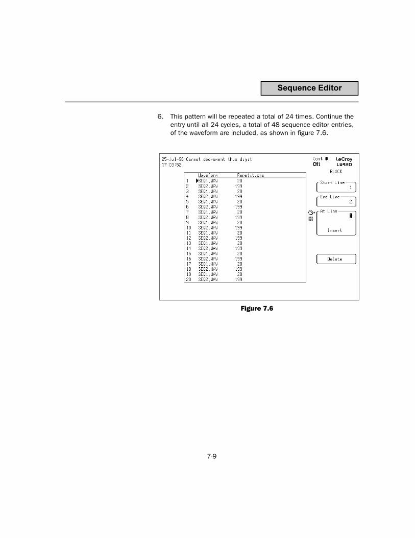
7-9

Sequence Editor

6. This pattern will be repeated a total of 24 times. Continue theentry until all 24 cycles, a total of 48 sequence editor entries,of the waveform are included, as shown in figure 7.6.

Figure 7.6

7-10

To simplify this process, we would normally define lines 1 and 2 asa Block and use sequence block edit to copy this pattern 23more timessee figure 7.7.

7. When complete, press the compile menu key to assemble andoutput the waveform.

The sequence mode will combine waveforms created with differentclock rates by selecting the optimum clock rate to generate all thewaveforms. Any error in waveform duration, incurred by this resam-pling, is reported in the Error column of the sequence editor. If acommon clock was used to generate the waveform segments theerror will always be 0.

View the output waveform on the oscilloscope at 0.5 s/div (1 Msample acquisition). Use zoom expansion to inspect the waveformat 0.2 ms/div and 50 µs/div.

Sequence Editor

Figure 7.7

7-11

Group Sequences

Introduction In the Group sequence mode all unique waveforms for allsequences included in the group sequence are loaded into theWaveStations high speed memory. The sum of the points in thewaveforms must be less than 1 Mpoint (Note: that waveforms muststart on a 512 point boundary so the actual sum may be less).Once the waveforms are all placed into high speed memory theAWG will start playing the first sequence in the list. See Table 7.1for a command summary.

The sequence will continue to play (in continuous trigger mode)until a sequence advance (defined below) is initiated from eitherthe front panel or by a remote command. The Wavestation willthen immediately advance to the next sequence in high speedmemory and play that sequence until another sequence advance isencountered. In addition to the auto advance feature, there is alsoa command to jump forward or backward to the nth group in thesequence.

The clock rate for all sequences must be the same. If the wave-forms of the sequences are not at the same clock rate, then thefastest clock is chosen and a dialog box will inform the user of this(just like with digital sequences).

Group Sequence

7-12

Creating a Group Sequence

The procedure to create a new Group Sequence is similar to thatused to create a new Sequence.

1. From the SELECT WAVE menu press the softkey New to viewthe NEW menu. Select the New CH1 SEQ item from this menu.

2. Use the appropriate softkey to select Group from the WhichType sub-menu that is displayed on the NEW CH1 SEQ menu..

3. The NEW CH1 SEQ menu will prompt you to enter a name forthe new sequence nd press Accept.. In this example the nameNEW GROUP SEQ2 was enteredsee figure 7.8.

3. Press the EDIT Key. When the EDIT menu appears select EditSequence to access the sequence editorsee figure 7.8.

4. The name of the first sequence of the group is then entered onthe EDIT SEQUENCE menu. Press the Insert softkey to enterthe sequence name in the group sequence file as shown infigure 7.8.

If you make an error in entering any of the information, selectthe line with the error and press the Delete menu key.

5. Continue to the next line until all sequences in the group areentered.

7. When complete, press the compile menu key to assemble andoutput the waveform. A message will be displayed when thecompile is completed sucessfully see figure 7.11.

Group Sequence

7-13

Group Sequence

Figure 7.10 Compiled Group Sequence

Figure 7.9 Edit Sequence MenuFigure 7.8

New CH1 SEQMenu

7-14

Group Sequence

Figure 7.11 Group Advance Operation

Using Group Sequences

When a Group sequence is selected the waveforms contained inthe sequences in the group are all placed into high speed memory.Upon completing the waveform loading, the WaveStation will beginplaying the first sequence in the list.

The sequence will continue to play (in continuous trigger mode)until a sequence Advance or Jump is initiated from either the frontpanel or by a remote command. The sequence pointed to by theAdvance or Jump will then immediately play until anothersequence command is issued.

ADVANCE ON Selects the channel the Advance, Jump, and Reset buttonscontrol.

ADVANCE Advances to the next sequence in the list. The current sequencewill stop wherever it currently is and the next sequence in the listwill begin playing

See the following figure 7.11for an example of ADVANCE.

7-15

Group Sequence

Figure 7.12 Group Jump Operation

JUMP TO Specifies which the sequence to jump to when the Jump button ispushed.

JUMP Jumps to the sequence specified by the value in Jump To. Thecurrent sequence will stop wherever it currently is and thesequence specified by the Jump To field will begin playing.

RESET Resets to the first sequence in the listequivalent to a jump to 1.The current sequence will stop wherever it currently is and the firstsequence in the list will begin playing.

See the following figure 7.12for an example of JUMP.

8-1

WAVEMATH8

WAVEMATHIntroduction Wavemath permits the user of the LW400 WaveStation to operate

mathematically on complete waveform files. The mathematicaloperations that are available are summarized in table 8.1.Mathematical operations such as smooth, integrate, and differen-tiate, that involve a single waveform, operate on the activechannel. In other words, to smooth the waveform in channel 1, itmust be the active waveform in the SELECT WAVE menu.Operations that require two waveforms (add, subtract, multiply,divide, convolve) forces the display to dual grid and a secondsource or reference wave to appear.

Table 8.1

Function Name Function DefinitionADD F(X) =Active Wave + Source 2SUBTRACT F(X) = Active Wave - Source 2MULTIPLY F(X) = Active Wave X Source 2DIVIDE F(X) = Active Wave / Source 2INTEGRATE (DC) F(X) = ∫ (Active Wave Median)INTEGRATE (AC) F(X) = ∫ (Active Wave)DIFFERENTIATE F(X) = d/dt (Active Wave)SMOOTH F(X) is an N point moving average

of the source

This is a form of digital filtering whichreduces the effective bandwidth of thesource.

Points is user selectable as 3, 5, 7, or9

Convolve

F(x)= ∫∞f1(t) f2(t-τ) dτ

−∞

Where f1 (t) = Active Wavef2 (t) = Source 2

*Note: Integrate, differentiate, and convolve are normalized tomaintain the initial peak to peak amplitude of the waveforms.

LW400 Math Functions

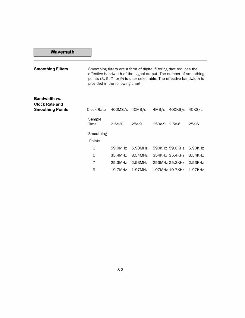
8-2

Smoothing Filters Smoothing filters are a form of digital filtering that reduces theeffective bandwidth of the signal output. The number of smoothingpoints (3, 5, 7, or 9) is user selectable. The effective bandwidth isprovided in the following chart.

Bandwidth vs. Clock Rate and Smoothing Points Clock Rate 400MS/s 40MS/s 4MS/s 400KS/s 40KS/s

SampleTime 2.5e-9 25e-9 250e-9 2.5e-6 25e-6

Smoothing

Points

3 59.0MHz 5.90MHz 590KHz 59.0KHz 5.90KHz

5 35.4MHz 3.54MHz 354KHz 35.4KHz 3.54KHz

7 25.3MHz 2.53MHz 253MHz 25.3KHz 2.53KHz

9 19.7MHz 1.97MHz 197MHz 19.7KHz 1.97KHz

Wavemath

8-3

Selecting the wave The following examples describe the use of these operations.

To ensure that the waveform of interest is active, it must beselected. This is described in detail in the section entitled

Waveform Viewing. The simplest way to tell if the desired wave-form is active is to look at the display. If you dont see yourwaveform, it is not active. In other words the display always showsthe active waveform.

Example: See figure 8.1 above

1. Push Select Wave

2. Select Channel 1 waveform

3. Select EQ27 WAVEFORM (in Project Examples.PRJ)

Wavemath

Figure 8.1 Selecting the wave

8-4

Performing Wavemath Performing Wavemath on this complete waveform is now a verysimple operation. The example below details integrating this wave-formSee Figure 8.2. Any of the functions that operate on a singlewaveform can be employed. To integrate this waveform perform thefollowing steps:

1. Push 2nd followed by WAVEMATH

2. Select the operation Integrate (This requires using the RotaryKnob or pushing the associated softkey and selecting from thelist of available functions)

3. Note: The difference between AC & DC coupling; DC integrationis done around zero whereas AC is done around the median ofthe waveform. Set the coupling to DC

4. Push Select All (note this assures the entire waveform isselected)

5. Push Accept (This is the action key that causes the mathemat-ical operation to be performed)

Wavemath

8-5

Wavemath

Figure 8.2 Integrating EQ27 WAVEFORM

Note: To undo the result simply push the UNDO button in thenumeric keypad group and answer OK.

8-6

Operating between the cursors It is not necessary to operate on entire waveforms. If you want to

operate on only a region of a waveform then the region of interestcan be isolated by using the time cursors. For example, if youwant to integrate only the fourth positive going pulse of the wave-form then enter the TIME CURSOR menu and bracket the firstpulse as shownin figure 8.3. The time cursors in this examplehave been set to 2.7 µsec for the left cursor and 3.5 µsec for theright cursor. This region is then isolated for the wavemath opera-tion. Refer to the section of the manual on Cursor manipulation formore details. The steps involved are outlined below.

1. Push Time Cursor

2. Select Time Left

3. Move the left cursor to 2.7 µsec

4. Select Time Right

5. Move the right cursor to 3.5 µsec

6. Return to the Wavemath Menu (2nd followed by Wavemath)

7. Set the coupling to AC

8. Push Accept

As before, it is possible to UNDO this operation by selecting andaccepting the UNDO command in the numeric keypad.

Wavemath

8-7

Wavemath

Figure 8.3 Isolating the fourth pulse for integration

Figure 8.4 Integrating the fourth pulse

8-8

Dual Waveform Math

Suppose we wish to operate on two waveforms with an appropriatemathematical function such as add, subtract, multiply, divide, orconvolution. Selecting one of these operations in the WAVEMATHmenu causes a new field to appear. This field is labeled Source 2and is where the selection is made for the second waveform to beused in the wavemath operation.

1. Push 2nd followed by WAVEMATHSee figure 8.5

2. Select Convolve

Wavemath

Figure 8.5 Dual Waveform Math

8-9

Wavemath

Figure 8.6 Selecting the second source

Practical Example of Dual Wave Math In this example, the active channel 1 waveform is differentiated

NRZ pattern. It is desired to convolve this NRZ pattern with asystem impulse response. The impulse response has been previ-ously measured or calculated and imported to the LW400 as awaveform called Convolve Wave and is shown in the bottom half offigure 8.6. Notice when a wavemath function that requires twowaveforms is selected, the screen splits so the second waveformcan be seen by the user. If the second waveform is not the correctone for the calculation, then push the Source 2 softkey and selectthe correct waveform.

As before, UNDO can be used to recover if a mistake has beenmade. It is also possible to use the cursors to bracket or isolate aregion of the active waveform to operate on. This operation is thesame as described above.

8-10

Wavemath

Figure 8.7 The result of convolving two waveforms

The final steps are as follows:

1. Push Select All

2. Push Accept

The result of the convolution of the two waveforms is shown on thetop trace of the display in figure 8.7.

9-1

ADDING NOISE9

Adding Noise To Waveforms The WaveStation allows users to add controlled amounts of noise

to waveforms in two ways. Synchronous pseudorandom noise canbe added using equations. Noise created in this way is repeatableand is the same every time the waveform is output.

On LW400 and LW400A models, internally generated, asynchro-nous noise can be added to the waveform (not available on theLW400B). This noise, uncorrelated with the waveform, is generatedby an independent pseudorandom noise generator and summedinto the output channels.

The LW400, LW400A, and LW400B models all include a rear panelBNC input for application of an external noise source.

Synchronous Noise Synchronous noise is added to waveform equations using either oftwo noise arguments, NOISE or GNOISE. Both NOISE and GNOISEare white noise sources; i.e. their signal energy is uniformly

distributed in the frequency domain. NOISE has a uniform ampli-tude distribution, while GNOISE provides a Gaussian amplitudedistribution. The statistical characteristics of the noise argumentsare summarized in the following table:

The random number generator used in the equation editor createsthe same noise sequence each time it is initialized at power up.Subsequent equation calculations, made without cycling power,return different noise sequences. In either case, the noise compo-nent added to each sample within the waveform is fixed and cannotbe changed without re-calculating. To recreate a waveform with adifferent set of noise components, simply recalculate the wave-form.

NOISE GNOISEFrequency Distribution Uniform Uniform

Amplitude Distribution Uniform Gaussian

Amplitude Range 0-1 V 0-1V

Mean 0.5 0.5

Standard Deviation 0.288 0.1667

Adding Noise

Figures 9.1 and 9.2 illustrate the use of GNOISE in adding noise toa damped sinewave:

Figure 9.1 Equation of a Damped Sine with additive noise

Figure 9.2 Damped Sine with additive noise

9-2

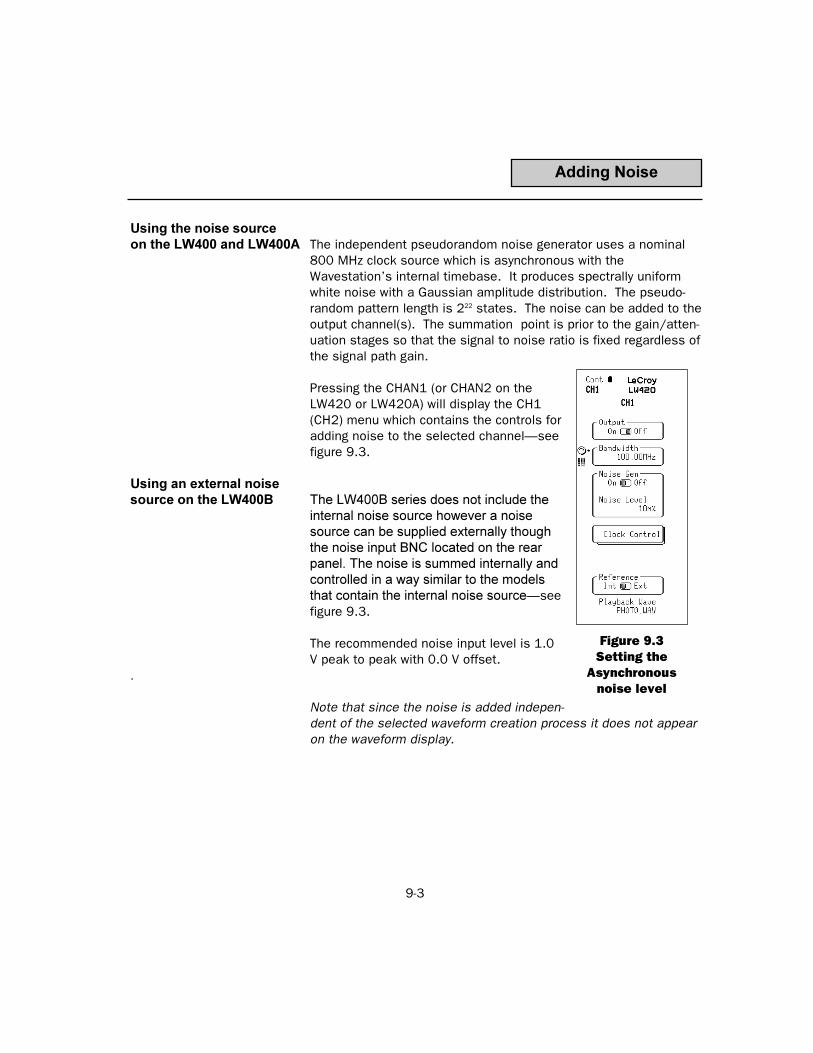
9-3

Adding Noise

Using the noise sourceon the LW400 and LW400A The independent pseudorandom noise generator uses a nominal

800 MHz clock source which is asynchronous with theWavestations internal timebase. It produces spectrally uniformwhite noise with a Gaussian amplitude distribution. The pseudo-random pattern length is 222 states. The noise can be added to theoutput channel(s). The summation point is prior to the gain/atten-uation stages so that the signal to noise ratio is fixed regardless ofthe signal path gain.

Pressing the CHAN1 (or CHAN2 on theLW420 or LW420A) will display the CH1(CH2) menu which contains the controls foradding noise to the selected channelseefigure 9.3.

Using an external noisesource on the LW400B The LW400B series does not include the

internal noise source however a noisesource can be supplied externally thoughthe noise input BNC located on the rearpanel. The noise is summed internally andcontrolled in a way similar to the modelsthat contain the internal noise sourceseefigure 9.3.

The recommended noise input level is 1.0V peak to peak with 0.0 V offset.

.

Note that since the noise is added indepen-dent of the selected waveform creation process it does not appearon the waveform display.

Figure 9.3Setting the

Asynchronousnoise level

9-4

Adding Noise

Noise Control Noise may be added to either or both channels in the dual channelmodels. The noise level is independently adjustable in eachchannel. The noise level is specified as a percentage of the noiseamplitude (in Volts RMS) to the currently selected waveformsamplitude (in Volts peak-to-peak) to a maximum of 9%. Thisassumes that the AWGs output bandwidth is set to the maximum,100 MHz, setting.

Example:

For A Signal Amplitude Of 1 Vpp And A Noise Level of 9%VNOISE=1 X 0.09VRMS (Gaussian Noise)

For Gaussian Noise the Peak to Peak Noise is:VNOISE(P-P)+6VNOISE RMS

Note: The noise source is uncalibrated, therefore the noise levelshould be measured and set to your specific requirements. ForGaussian Noise: VRMS=1 (sigma) and Peak to Peak=6 X VRMS

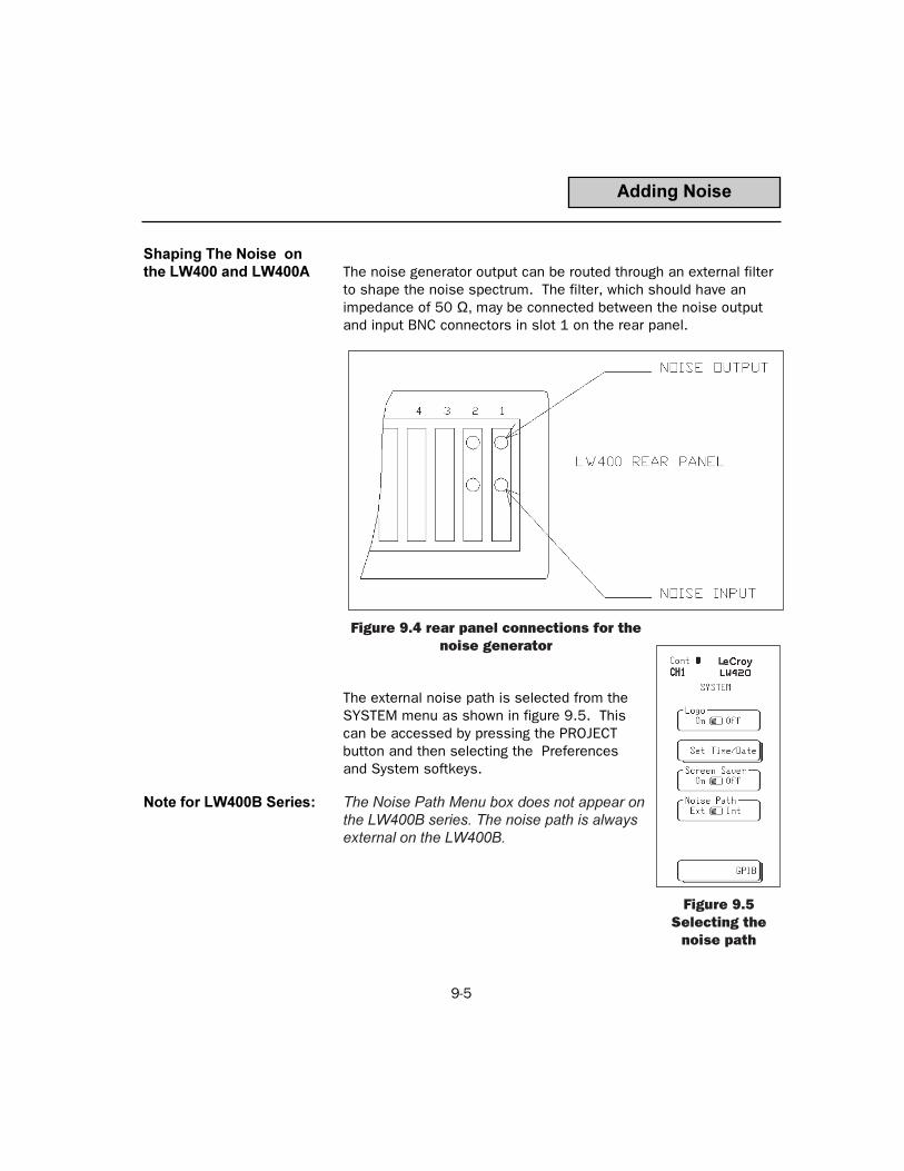
9-5

Adding Noise

Shaping The Noise onthe LW400 and LW400A The noise generator output can be routed through an external filter

to shape the noise spectrum. The filter, which should have animpedance of 50 Ω, may be connected between the noise outputand input BNC connectors in slot 1 on the rear panel.

The external noise path is selected from theSYSTEM menu as shown in figure 9.5. Thiscan be accessed by pressing the PROJECTbutton and then selecting the Preferencesand System softkeys.

Note for LW400B Series: The Noise Path Menu box does not appear onthe LW400B series. The noise path is alwaysexternal on the LW400B.

Figure 9.4 rear panel connections for thenoise generator

Figure 9.5Selecting the

noise path

10-1

PROJECT STRUCTURE10

The project structure of the WaveStation is intended to provide alogical place to group waveform files and certain system parame-ters. It is intended to facilitate the use of the instrument in a multiuser environment where different users can have their own uniquedirectory of waveforms. Within the user directories, waveform filescan be stored along with certain system setup files that define theconfiguration of the LW400 at start up or initialization.

The project structure can be likened to the file manager in moderncomputer operating environments such as windows in that itgives the user an easy way to access a hierarchy of directories,called projects in the WaveStation, and to move files into and outof each project directory in WaveStation, as well as between projectdirectories. It also gives the user a way to write protect his or herfiles should it be necessary.

The multi disk file management capability provides support forimporting and exporting large waveforms and projects.

Figure 10.1 The Project Menu

10-2

Project Structure

Figure 10.2 The Role of the Project Manager

Table 10.1 Selections in the Project menu

New Assign a name to a New Project

Open Choose an existing project from a list and open it

Save Will save changes to current project or save as to change name

Delete Delete a waveform, sequence, equation or project

Import Get something from various available sources (see below)

Export Send something to various available destinations (see below)

Preferences Sets a myriad of initial conditions (see below)

Factory Default Set to known statedefault settings

YOUR

PROJECT

MY

PROJECT

THEIR

PROJECT

PPRROOJJEECCTT

MMAANNAAGGEERR

PPRROOJJEECCTT

MMAANNAAGGEERR

MATHCAD

MATHLAB

PSPICE

OTHER PROJECTS

FLOPPY DISK FILES

SCOPE FILES

LW400 FILES

EASYWAVE EQUATIONS

LeCroy SCOPE FILES

10-3

Project Menu

New This menu is used to create and name a new project.

Open This menu is used to select an existing project.

Save On entry to the menu this field contains the name of the openproject. If a name is entered in the Save As menu (see below) thenthis field contains that name.

Save As This menu is used to change the name under which the currentproject will be saved.

Save It Saves the current project. Note: if the project is write protectedthen the user will be told its a write protected project and abortthe save operation. If a new name was entered for the project(Save As) then a new project is created from the current project.This includes all waveforms, sequences, equations and projectpreference settings. The old project is closed (no prompt is given ifsettings have changed) and the new project is opened.

Project Save

10-4

Delete This is the only place to delete projects, waveforms, sequences,equations, or DSO files. Everything comes in and out of theLW400 through the project menu. The current and default projectsmay not be deleted. Anything in a write protected project may notbe deleted. After delete is pressed then a message appears toverify delete.

What This field contains the different types of objects that can bedeleted; Projects, Waveforms, Sequences, Equations and DSOfiles. This field dictates what type of objects are shown in the nextfield. The rotary knob is attached to this field.

Projects This field contains the objects that can be deleted (dependent onthe What field). The label for this field changes in accordance withthe What field. If the What field contains Sequence the label willbe Sequences. The different labels for this field are: Projects,Waveforms, Sequences, and Equations.

Delete This is the action softkey that begins the delete operation (depen-dent on the Are You Sure button) of the object in the fieldsdescribed above. If the object is write protected it will not bedeleted and the appropriate message will be given to the user.

Project Delete

10-5

Project Import

ImportRefer to section 12 for additional details

What The following object types that can be imported into a project: LW4XX Waveform, LW4XX Sequence, LW4XX Equation, LW4XXProject, EasyWave Wave, EasyWave Wad, EasyWave Seq,LeCroyScopeFile, MathCad File, PSpice File, MatLab File,ASCII(Data,Hex,Binary), Spread Sheet File or DSO file.

From This is the location of the object to be imported.Objects can be imported from other projects, or afloppy disk.

Path/Project This is the actual path to the objects. Theappearance of this field depends on the Fromfield. If the From field displays Another Project,then this field is a list of valid projects. If theFrom field displays Floppy Disk, then this field isa menu labeled Path. The path submenupermits selection of the floppy disk subdirectory.

Source File This is the object to be imported. The listcontains the objects found in the Project/Path.

Target File This is the name assigned to the importedobject. It will duplicate the name in the SourceFile field until it is changed with Import As (seebelow) at which point it will be the name entered.

Import As Use this menu to enter a new name for theobject to be imported.

Options Pressing the Options softkey displays a menu used to selectop-tions to process waveforms during import.

Import Press the IMPORT softkey to import the object in Source File intothe current project with the name in Target File. If it is not anLW4XX object then it will be converted to one because only LW4XXobjects are stored in the WaveStation.

Figure 10.3The Import

Menu

10-6

Project Import

Export

To This is the location to export the object to. Objects can only beexported to a floppy disk. Transfers between projects are handledby Import.

Project/Path This is the actual path to store the objecti on thefloppy disk. The path menu is shown below.

What This field specifies what is to be exported,choices are Projects, Waveform, Sequence,Equations, or DSO files.

Format This field only appears only if a waveform isbeing exported. This is the format in which toexport the object in. The valid choices are:LW400 Waveform, MathCad, Matlab, spreadsheet, or PSpice (PWL)

Source File This is the object to be exported. The listcontains the objects of the type in the currentproject.

Target File This is the name to be used when the object isexported. It will duplicate the name in theSource File field unless it is changed with ExportAs (see below) at which point it will be the nameentered.

Export As This menu allows the user to enter a new name for the object to beexported.

Export This is the action softkey that exports the object in Source File tothe disk with the path as dictated by the Project/Path field in theformat of the Format field with the name in Target File.

Figure 10.4The Export

Menu

10-7

Project Export

Preferences The preferences menu, shown in the followingfigure, offers the choice of entering the Systempreferences menu or enabling Write Protect onthe current project.

System Menu Pressing the System softkey will result indisplay of the SYSTEM menu shown in figure10.6.

The functions of the SYSTEM menu softkeys aresummarized in table 10.2 shown below.

Write Protect This On/Off switch write protects the entireproject. All waveforms and settings will be writeprotected. New waveforms, however, may be created, or imported.Waveforms may also be exported. Note: that any waveform that iscreated in a write protected project is automatically write protectedonce it is saved.

Enable Undo Selecting Yes/No with the softkey enables/disables the undobuffer operation. This can speed up menuchanges on very long waveforms

Figure 10.5 ThePreferences

Menu

Figure 10.6The System

MenuTable 10.2

Softkey FunctionLogo (ON/OFF) Turn The LeCroy LW400 logo on or off

Time/Date Turn real time clock display on or off. Sets time and date.

Screen Saver (ON/OFF) Enables screen saver

Noise Path (EXT/INT) Selects internal or external path for asynchro-nous noise source. The external path is used tosupply an external noise source and to filter orcolor the noise. On the LW400B, External isalways selected.

GPIB Used to set GPIB address of the LW400

11-1

HARDCOPY11

Hardcopy

Format Graphics or Printer

Type Graphics:.PCX., .TIF, .BMPType Printer: Epson MX/FX.LQ, HP LaserJet II

and HP ThinkJetQuality Proof of Draft (Graphics Only)Destination Centronics, Floppy, GPIB (Printer)

Filename Enter the file name (Floppy only)Index Filename.index starting with .000Auto/Incr Yes/No turns on incrementing of theindex

Table 11.2 Setup Options for Printer output only

Size Presentation (4.26" X 2.66")Notebook (5.53" X 5.33") (Valid for HPLaser Jet II only).

Quality Proof/Draft: Valid for Epson LQ, HP ThinkJet, & HP LaserJet only.Page Feed On/Off: On generates a page feed after the waveform is printed.

Table 11.1 Hardcopy Options

Figure 11.1Hardcopy Menu

Many different styles of printers and graphics files are directlysupported. The hardcopy setup menu system is accessed bypressing 2nd (red button) followed by the Time Cursor button(HARDCOPY is in red) in the View Group on the front panel next tothe Rotary Knob. The menu displayed is shown in figure 11.1. Theprinter types, formats and options are shown intables 11.1 and11.2.

11-2

Hardcopy

Hardcopy Output LW400 hardcopy output provides screen images to graphics file orprinter. If the output format is capable of high resolution, theoutput quality can be selected as either proof or draft.

Draft output provides black/white output only: Trace, Grid, andText, printed as black on white.

Proof output takes advantage of the extra available output resolu-tion to provide a differentiation between trace data and Grid usinggray scale intensity.

Choosing the Portfor Hardcopy If hard copy is to be performed directly to a printer then it is neces-

sary to connect the printer to one of the available output ports. TheCentronics or GPIB port are both available as printer destinations.

File names The filename will be HCOPY with a 3 digit index. The extension willbe .WAV if it is a printer file or the appropriate graphics file formatextension if it is a graphics file. Example: HCOPY000.TIF

* for additional setup information, see the following sections enti-tled Interface Basics describing these ports and how toconfigure them.

11-3

Printers

Using Hardcopy for Printing

The HARDCOPY softkey menu is shown in figure 11.1. To send apicture of the current display to your printer perform the followingsteps.

1. Set FORMAT to PRINTER

2. Set TYPE to (As defined below)Types: Epson MX/FX Epson compatible 9 Pin Dot matrix

printerEpson LQ Epson compatible 24 Pin Dot matrix

printerHP Laser Jet II HP Laser Jet Series II and

compatibles (also Laser Jet IV)HP ThinkJet HP ThinkJet Compatible

3. Setup OPTIONS (as defined below)

Size: Notebook: 4.2" x 6.0" (10.66 mm x 7.62 mm)Presentation: 8.4" x 6.0" (21.33 mm x 15.25 mm)

Page Feed:On: Automatic form feed for each pageOff: Requires manual or externally generated

form feed.Quality: Proof: High qualitygray scale presentation of

graphic element.Draft: Fast printing black/white only.

11-4

Graphic Files

Storing Hardcopy to a Floppy Disk

In order to use the hardcopy menu to store a screen image to thefloppy disk, select destination floppy in the hardcopy menu. Thismenu permits selection of either printer format files or graphicsformat files. The steps are as follows.

1. Select 2nd followed by Hardcopy2. Select Format Printer or Graphics file3. Select Type from the available options4. Select setup option (printer only)5. Select Index6. Set Auto Incr. to yes or no7. Select execute

This final step causes an image of the screen to be stored to thefloppy disk in whatever format was selected.

Figure 11.2 Storing to Floppy Disk

11-5

File Naming

File Naming Conventions

The LW400 uses a standardized scheme for filenames whenstoring and recalling files from disk.

All files adhere to the DOS convention of an 8 character name and3 character extension. The default extensions are defined below foreach of the data formats supported by LW400.

.PRN Hardcopy Printer format file

.PCX PC-Paintbrush compatible graphics file

.BMP Windows Bit-Map compatible graphics file

.TIF Tag-Image format compatible graphics file

Many of the Hardcopy file formats supported in LW400 can alsoaccommodate a unique numeric index to facilitate an auto-incre-menting filename.

When the auto-increment feature is supported, for a particular fileformat, a three-digit numeric index is used for the last 3 digits ofthe 8 character filename.

Disk Paths The IMPORT, EXPORT, and HARDCOPY system use a defaultdirectory (or paths) for all file related operations. The default direc-tory is specified in the PATHS menu. This menu is accessible fromwithin the EXPORT or IMPORT menus, found under PROJECT.

12-1

IMPORTING & EXPORTING12

IMPORTING AND EXPORTING WAVEFORM FILES

The LW400 WaveStation provides multiple formats to communicatewith other sources of waveform data. By definition, importing andexporting means bringing a waveform file into or out of a currentproject from either another project or on a floppy disk. The Importand Export menus are found under the Project Menu. In order toSelect Import or Export, push the Project key located on the leftside of the floppy disk drive on the front panel of the WaveStation.After this select either Import or Export. In all that follows, Importwill be used as an example. The export operation is in general, theinverse of the Import operation.

Figure 12.1 The Import Menu

12-2

Import

Information Requested On Import

The Wavestation will prompt the user for time and/or amplitudeinformation if it is not evident from the file being imported or it mayneed to perform rescaling of the imported data. This may occur forEasywave files without associated setup files, ASCII (.DAT) files,Matlab, or spreadsheet files.

Time and AmplitudeRange Request When necessary the Wavestation will prompt you to enter new

time and/or amplitude informationEnter Newor to use thecurrentUse CurrentWavestation settings as shown in figure12.2.

Figure 12.2 The Time/Amplitude Warning Box

12-3

Import

Figure 12.3 Entering time information

Time and Amplitude Entry If Enter New was selectedsee figure 12.2 the menu shown infigure 12.3 will be displayed, however only the necessary informa-tion will be requested. Time is entered as Time/Point and theamplitude range is specified by entering minimum and maximumvoltage levels.

12-4

Import

Figure 12.4 The Rescale Warning Box

Rescaling If the Wavestation determines that the data requires rescaling priorto import a prompt will appear as shown in figure 12.4. Twochoices are provided for rescaling of the waveform during import:

1. Choosing Preserve Time automaticaly sets the sample clock toassure that the duration of the waveform generated on theWaveStation equals that of the waveform file imported.

2. Preserve shape assures that the generated waveform has thesame shape as the waveform file imported, however the durationof the waveform may not be the same..

12-5

Import

Import Options

Oversample Wave In order to edit a waveform on the WaveStation, the waveform mustbe sufficiently oversampled. Many of the editing functions utilizesignal processing using a sinx/x interpolator. The interpolator willcreate significant ringing if the data is notoversampled. If this field is set to Yes thenthe waveform will be checked for discontinu-ities and if found they will be fixed bypassing the discontinuity through a lowpass filter assuring sufficient oversampling.

If No is chosen then the data will not bechecked for discontinuities. If the dataimported is not sufficiently oversampled,editing operations cannot be applied to thewaveform until it is oversampled. If youattempt to edit an undersampled waveform,the Wavestation will prompt you with amessage allowing you to oversample thewaveform. After the waveform has be over-sampled, editing operations can beperformed.

Advantages of not oversampling are: Faster edges can be achievedsince more then one point on and edge is not required; You canimport a waveform without modifying the points. This may provevaluable in some situations.

WAVES ARE Choose to consider the waveforms imported as a single shot wave-form or a continuous waveform (last point wrapped to the first).Continuous waveforms are displayed with the ends wrapped in adimmer shade on the screen. The discontinuity check will checkfor a discontinuity between the end and the beginning of the wave-form. This makes the presumption that when the Wavestationreaches the end of the waveform it will jump to the beginning andplay the first point. If the waveform is only to be played once(single shot) or, is part of a sequence where wrapping the endsmight be an incorrect thing to do, single should be selected for thisfield.

Figure 12.5Import Options

Menu

12-6

Import

Import/Export ofLarge ASCII Waveforms Multi-disk importing is supported for LW4XX waveforms and other

files including: Spreadsheet, Mathcad, MatLab, and PSpiceformats. When the import function reaches the end of a file forone of these formats you will be prompted, questioning if there ismore data or not. If the answer is yes, you will be prompted toselect another file. The default name will be the original name ofthe file being imported but with a .000 extension. The next fileextension will be .001, then .002 etc. If this is not the name ofthe next portion of the waveform the user can enter the name usinga standard filename entry menu (like import as menu).

When the Wavestation exports large waveforms the first disk islabeled with a name entered by the user (i.e. user.txt). The nextdisk will be automatically labeled user.000 then user.001 etc.

12-7

Import

The Import Menu Sourcesof Waveforms to Import There are many sources of waveforms to import (export). The list

of available options is arrived at by selecting what in the Import(Export) menu. Selections include:

LW4XX Waveforms

LW4XX Sequence

LW4XX Equation

LW4XX Project

EasyWave Wave

EasyWave Wad (dual waveform file)

EasyWave Sequence

Spreadsheet (useful for any text file of values)

MathCad

MatLab

PSpice (maximum of four nodes in simulation output)

ASCII Data (integer values between 0 and 255)

LeCroy Scope File

DSO Config File (creat configuration for other scopes)

Note: units equipped with the LW400-09 digital ouput option wilalso accept digital EasyWave files, ASCII Hex, and ASCII Binary.See the Appendix covering LW400-09 for additional details.

12-8

Import

Figure 12.6 Choices for Import (Export)

Import What Menu The menu shown in figure 12.6 is displayed upon selection ofWhat by pressing the softkey on the front panel. The selection ofthe object type to import, is made by pressing the approriatesoftkey.

12-9

Spread Sheets

Communicating With Spread Sheets

Importing from the spreadsheet to WaveStation Creating waveforms from data in spreadsheets (such as Microsoft

Excel) requires files in comma delimited, ASCII format.

The spreadsheet import selection also enables import of filescontaining values in one or two columns.

For a file containing two vectors, or arrays, the first array will beassumed to be time and the second array will be amplitude. So,the arrays are read in as time value, amplitude value.

For a single column or array, it is assumed to be the amplitudearray and a question will be asked to prompt you to enter a timevalue.

Wavestation automatically scales the amplitude to assure thefull digitizing range is used. If the peak to peak amplitude is inthe range of ± 5.0 volts the signal amplitude will correspond tothat of the data imported. The amplitude can easily be adjustedvia the front panel and saved under a name of your choice.

Exporting From WaveStation to the spreadsheet If a file is exported from the WaveStation as a spreadsheet file,

both amplitude and time values are stored for each waveformpoint. To import the file into a spreadsheet program enter thespreadsheet and import the file as a text (filename.txt) file.

Note in Excel, for example, this also means selecting the commaas the delimiting item. Enter Excel and pull down the filemenu. Select open. In the open dialogue box select textand then select comma. Note these file formats are alsocompatible with other apreadsheet programs as well as databaseprograms such as Microsoft ACCESS.

Refer to your softwares manual for specific instruction regardingimporting common delimited ASCII Files.

12-10

Communicating with MathCad

Importing From MathCad to WaveStation From MathCad, to prepare a file for importing into the WaveStation

it is stored with the WRITEPRN(FILE) command of MathCad. Thisproduces a data file named FILE.PRN. This file will be read directlyby the WaveStation. Store the file on a floppy disk and insert thedisk into WaveStation. In the figure below, a file namedMY_FILE.PRN has been stored on the floppy disk. It is ready to beimported to WaveStation.

MathCad

Figure 12.7 Importing From Mathcad

12-11

Exporting from WaveStation to Mathcad

The steps to export a data file from WaveStation to MathCad areas follows:

1. Export a waveform file to a floppy disk using MathCad (.PRN)formatSee figure.

2. Storing the desired waveform in MathCad format produces astructured data file with the .PRN extension. Start MathCad andinsert the disk containing the MathCad file into the computer.

3. Use associate filename found in the MathCad FILE pull downmenu to associate the LW400 file with a MathCad matrix vari-able, LS_DATA.

4. Use the READPRN(LS_DATA) command in MathCad to read thedata from the file into matrix LS_DATA.

MathCad

Figure 12.8 Exporting a waveform to Mathcad

12-12

COMMUNICATING WITH PSPICE

PSpice is an analog simulation package that can be used togenerate waveforms from circuit models. PSpice has severaldifferent methods of generating or storing files. It generates filesin piecewise linear format (.PWL) or .OUT format. WaveStationgenerates .PWL files for exporting to PSpice and accepts .OUT filesfor importing from PSpice.

Exporting from WaveStation to PSpice

WaveStation generate files in the .PWL or piece wise linear format.The files so generated are used to describe a voltage source wave-form in PSpice and must be included in the Spice net list. The filegenerated from the WaveStation must be included in the appro-priate PSpice directory.

Importing to WaveStation from PSpice

The PSpice file must be stored as a .OUT file. Up to four nodescan be included in the file. If more than one node is present,WaveStation will ask which node to import. Import begins at thepoint in the file where the first character is a numeric value.If a linecontains a numeric character in the first colum prior to this pointan import error will occur.

**** TRANSIENT ANALYSIS TEMPERATURE = 27.000 DEG C******************************************************************************TIME V(1) V(2) V(3) V(4)

0.000E+00 0.000E+00 -6.590E-26 6.590E-26 0.000E+001.000E-05 3.139E-01 3.314E-03 1.611E-04 1.158E-032.000E-05 6.266E-01 9.882E-02 3.136E-03 3.399E-023.000E-05 9.365E-01 3.273E-01 1.027E-02 1.125E-014.000E-05 1.243E+00 5.915E-01 1.852E-02 2.034E-015.000E-05 1.544E+00 8.678E-01 2.715E-02 2.983E-016.000E-05 1.840E+00 1.146E+00 3.584E-02 3.939E-017.000E-05 2.128E+00 1.421E+00 4.444E-02 4.885E-0

PSpice

12-13

Communicating With MatLab

MatLab is a matrix oriented mathematical analysis program that isin common use for generating complex waveshapes. MatLabgenerates two different waveform format files. Either can containmultiple matrices. The first is a standard ASCII file. The second isthe .MAT file which is a binary file. Currently WaveStation supportsthe ASCII file format (identified by a .DAT extension) from MatLab.

Exporting to MatLab from WaveStation In order to export a file to MatLab from WaveStation, it is only

necessary to export it in MatLab format. The WaveStation exports aone dimensional array of amplitude values. If the wavefile name ismyfile, it will be exported as myfile.dat and can be importeddirectly into MatLab using the Load command.

Importing from MatLab to WaveStation

1 dimensional arrays The case of the 1xN or Nx1 array is handledsimilarly. In MatLab, save the file with thecommand string save yourfile.dat arrayname -ascii. This produces a file with name yourfilefrom the MatLab array arrayname.

Load the floppy disk with this file into theWaveStation and import it directly. In the caseof the one dimensional array, only amplitudevalues are assumed. The timebase that will beassociated with this file is the currentWaveStation clock setting.

Import Steps 1. Push Project2. Push Import 3. Select What and then MatLab4. Select From and then Floppy5. Select Sourcefile and Yourfile6. Push Import

See figure 12.9 at right.2 dimensional arrays

MatLab

Figure 12.9 Importing From

MatLab

12-14

column matrices There are two formats for 2 dimensional arrays: column format orrow format. In column format (there are 2 columns of n elementseach), The WaveStation examines the first two elements of the firstcolumn and extracts the timebase. If the first column had valuesx1, x2, x3, ..., then the time step is taken as x2 - x1 = t. If this is aninvalid time, then the user is prompted and asked whether topreserve time or shape. Preserving shape will cause theWaveStation to use its current clock setting, whereas preservingtime causes WaveStation to resample the waveform thuspreserving the overall waveform duration.

row matrices It is possible to save the data file in two arrays that are effectively2 individual 1xN arrays. The format of the MatLab command issave yourfile.dat array1 array2 -ascii. This produces two individualarrays that can be examined by the WaveStation. In this case,array1 is assumed to be the time array while array2 is the amplitudearray.

This file is imported into WaveStation just the same as the singlearray. However this presents an interesting possibility for theinformed user. WaveStation will only examine the first values ofarray1 to determine the amplitude values. If the remainder of thearray is empty, it is of no consequence with one exception. Theremust be a third value in the array which is used solely to deter-mine that it is a row array and not a column array. So in the case ofdescribing the function with two independent arrays, if the values inarray1 are array1 = (0,t,x) where t is the requested delta time and xis any number, then the correct time information can be passed toWaveStation while achieving a considerable savings in the file size.

MatLab

12-15

Easy Wave

Communicating With EasyWave

EasyWave files are directly imported to WaveStation. If theEasyWave file has an associated setting file (filename.set) then theWaveStation will read the time, amplitude and offset informationfrom the settings file. If an EasyWave waveform file has no associ-ated setup file the LW400 will look for a default setings file,IMPORT.SET. If no settings file is present, the WaveStation asksthe operator to input a time increment.

12-16

LeCroy DSOs

Communicating with LeCroy Digital Oscilloscopes

Any LeCroy digital oscilloscope that has a floppy disk drive cangenerate a WaveStation compatible file. This file can then beimported into the WaveStation using the file import menu. UseLeCroy Scope File from the What field. Note this is different thanthe Get From Scope command that is implemented in the wave-form editor under Insert Wave which requires a GPIB cablebetween the oscilloscope and the WaveStation.

12-17

Import Other Files

Importing ASCII Data Files ASCII Data files consist of integer values between 0 and 255,

encoded as ASCII numbers separated by spaces or commas. TheWaveStation will prompt for the voltage range and time per point.

DSO Configuration Files DSO configurations file with .DSO extension, are used to describe

the key parameters of digital oscilloscopes needed to input wave-forms. For more information contact LeCroy for additionalinformation.

12-18

Export

Exporting to Floppy Disk

1. Press Operation key PROJECT.

2. Press softkey EXPORT then select the destination of the databy selecting TO floppy disk.

3. Press softkey WHAT and select type of file to be stored.

4. Press the FORMAT softkey and select the choices of how thewaveform will be stored (LW400 Waveform, MathCad, PSpice,etc.).

5. The TO softkey will default to Floppy.

6. Select the source file and TARGET FILENAMES.

7. Press EXPORT and the waveform will be stored. If more then 1floppy disk is required you will be prompted to insert additionaldisks.

8. The TARGET FILENAME can be changed to any desired file-name by pressing the EXPORT AS menu key and then enteringthe desired file name.

13-1

SAMPLE CLOCK

Sample Clock Introduction

The LW400A and the LW400B Models have a sample clock thatis continuously variable while the LW400 models have a clock vari-able over specific decade ranges.

The clock menu is used to set the clock related options for theselected waveform. The menu and range of the clock are differentdepending on whether or not the continuous clock option isinstalled. The continuous clock has a range from 6kHz to 400MHz.The standard clock has the following frequency ranges: 355MHz -400MHz, 35.5MHz - 40MHz, 3.55MHz - 4MHz, 355kHz - 400kHz,35.5kHz - 40kHz.

There are three parts to this section.

Refer to the LW400 Clock Setting part if you are using anLW410 or LW420.

Refer to the LW400A/B Clock Setting part if you are using anLW410A, LW420A, LW410B, or LW420B.

The External Reference part is common to all models anddescribes setting up the Wavestation for use with a 10 MHzexternal clock reference.

13

13-2

LW400 Clock Setting

LW400 Clock Setting

Setting The SampleClock Rate When a waveform is created or imported, the LW400 determines

the clock rate and number of samples required to generate thewaveform with the correct timing and optimum output filtering.Therefore, a logical sample clock rate is associated with everywaveform generated in the LW400. Channel 1 is setup as themaster channel, the waveform in channel 1 determines the phys-ical clock rate for the AWG. Whenever a waveform is selected asthe channel 1 waveform the sample clock associated with thatwaveform is used to set the internal clock rate of the LW400.

There are two methods ofchanging a waveforms sampleclock rate.

Clock Set Method 1 1. Press the CHAN1 button onthe front panel to access theCH1 menufigure 13.1.

2. Press the Clock Controlsoftkey to access the ClockControl menufigure 13.2.

3. Select the desired value ofthe Max Clk Value or ClockRate in the Clock Controlmenu.

The clock parameter fields inthe CH1 menu control theclock hardware of the LW400directly and affect the wave-forms in both channels of theLW400.

Figure 13.1Clock

Selection onCH-1 Menu

Figure 13.2Setting the

Clock Decadeand Frequency

13-3

LW400 Clock Setting

The clock rate is normally set automatically by the LW400. TheClock Control menu allows users to override the normal operationof the LW400 and manually set the logical clock rate, associatedwith the selected waveform. If channel 1 is selected as the activewaveform, then the CLOCK menu sets both the logical clock rate ofthe waveform and the system clock rate. Otherwise, if the scratchpad or channel 2 editor is selected, the CLOCK menu only affectsthe logical clock rate of the waveform.

Clock Set Method 2 The second method of changing the clocksetting for the currently selected waveform is asfollows:

1. Access the Clock Control menu from thefront panel by pressing the red 2ND buttonthen the CLOCK button(the alternate function ofthe TIME button). The CLOCK menu is shown infigure 13.3.

2. Select the Max Clk Value or Clock Rate inthe Clock Control menu.

The menu items associated with setting theclock rate, using either method, are similar anddescribed on pages 13-4 and 13-5.

Figure 13.3 TheClock Menu

13-4

LW400 Clock Setting

AUTO CLOCK SET The Auto Clock Set selection determines if the sample clock ratecan be automatically varied as each new waveform is created orimported or if it is fixed at a single value. If this field is set to Yes,the WaveStation automatically selects the best sample rate inorder to achieve the required duration. With this field set to No,the clock rate is held at the user set frequency and the number ofsamples is varied to set the waveform duration. In general, thevariable clock rate allows more flexibility in achieving the desiredwaveform duration. In fixed mode, the achievable waveform dura-tion will always be integer multiplies of the clock period.

MAX CLK VALUE This field is used to set the maximum value for the clock rate. TheMax Clk Value is a numeric field that can be set to one of thefollowing: 400MHz, 40MHz, 4MHz, 400kHz, or 40kHz to match theavailable output filters of 100 MHz, 10 MHz, 1 MHz, 100 kHz, 10kHz respectively.

MIN CLK VALUE The Min Clk Value is an information field that displays the currentminimum clock rate value.

CLOCK RATE If Auto Clock Set is set to No, the clock frequency shown in theClock Rate field is fixed, and will not change unless anotherfrequency is manually selected. If Auto Clock Set is set to Yes,the current clock frequency is shown in the field. The clock ratecan be adjusted when either setting is selected, however, if theLW400 is in auto clock mode then the clock rate may changewithout notification.

The Clock Rate is set using the numeric keypad or the rotary knob.The frequency can be set with a 1 Hz resolution within the decaderangesee table 13.1displayed by the Max Clk Value and MinClk Value fields.

Note that if the LW400-09A digital output option is installed thenadditional clock ranges are available for use with digital wave-forms. See the appendix covering LW400-09A for additionalinformation.

Clock Rate In Dual Channel AWGs Waveforms selected in channel 2 of the LW400

are generated using the same sample clock aschannel 1. For this reason, if the waveform wascreated at a different clock rate then a warningmessage, Please resample channel 2 willappear. Press the button labeled CHAN 2 todisplay the CH 2 menu, shown in the accompa-nying figure. Press the Resample softkey, thewaveform in channel 2 is resampled using thecurrently set clock rate.

13-5

Figure 13.4ResamplingChannel 2

LW400 Clock Setting

Decade Lower Limit Upper Limit400 MHz 355 MHz 400 MHz40 MHz 35.5 MHz 40 MHz4 MHz 3.55 MHz 4 MHz400 kHz 355 kHz 400 kHz40 kHz 35.5 kHz 40 kHz

Table 13.1 Clock Decades

13-6

LW400A/B Clock Setting

LW400A/B Clock SettingPress the 2nd then CLOCK buttons on the front panel to enter theCLOCK CONTROL menu.

OPTIMIZE CLOCK (Set to Yes) This field gives the user a single button to press that sets the clock

menu up in a way that will best optimize the clock. SettingOptimize Clock to Yes on the menu sets Auto Clock Set to Yesand Limit Clock to Yes. This causes the LW400A/B to automati-cally pick the best clock for edit operations and limits that clock toa clock rate that has a matching filter.

The clock can be modifiedwithin the rangeshown on the menuby changing the value inthe Clock Rate sub-menu shown.

The Maximum clock rate can be changed bychanging the value shown in the Max ClkValue sub-menu as shown. If a value isselected that is not within an allowable clockdecade, the WaveStation will select a valuewithin the decade.

When set for optimized clock, the LW400A/Bclock operation is similar to that of theLW400.

Figure 13.5Clock Control

13-7

LW400A/B Clock Setting

OPTIMIZE CLOCK (Set to No) Setting Optimize Clock to NoWith the continuous clock option

enables full control of the continuously variable clock. With thissetting the two menus available are as shown in figure 13.5 andFigure 13.6

AUTO CLOCK SET The Auto Clock Set selection determines if the sample clock ratecan be automatically varied as each new waveform is created orimported or if it is fixed at a single value. If this field is set to Yes,the WaveStation automatically selects the best sample rate inorder to achieve the required duration. With this field set to No,the clock rate is held at the user set frequency and the number ofsamples is varied to set the waveform duration. In general, thevariable clock rate allows more flexibility in achieving the desiredwaveform duration. In fixed mode, the achievable waveform dura-tion will always be integer multiplies of the clock period.

LIMIT CLOCK The WaveStation has five built in filters that are designed to matchthe decade ranges of the standard clock. Using one of theseclocks and the corresponding filter will produce the best output.Selecting Yes in the Limit Clock to Internal Filter Ranges? menu,limits the clock that can be set (by both the user and the automaticclock select feature) to only clock ranges that have a correspondingfiltersee figure 13.6. If this field is set to No then all achievableclock ranges can be setsee figure 13.5.

MAX CLK VALUE The Max Clk Value field changes depending on the state of theLimit Clock field. This field sets the maximum value for the clockrate. With the Limit Clock set to Yessee figure 13.6, this fieldis a numeric field that can be set to one of the following: 400MHz,40MHz, 4MHz, 400kHz, or 40kHz to match the available outputfilters of 100 MHz, 10 MHz, 1 MHz, 100 kHz, 10 kHz respectivly.

With Limit Clock set to Nosee figure 13.5, this field is an infor-mation box that displays what the Maximum clock rate is and cannot be changed.

MIN CLK VALUE This is an information field that displays the current minimum clockrate value.

13-8

CLOCK RATE If Auto Clock Set is set to No, the clock frequency shown in theClock Rate field is fixed and will not change unless anotherfrequency is manually selected. If Auto Clock Set is set to Yes, thecurrent clock frequency is shown in the field. The clock rate can beadjusted when either setting is selected, however, if the LW400 isin auto clock mode then the clock rate may change without notifica-tion.

The user can enter the sample clock rate using the numeric keypador the rotary knob. The frequency can be set with 1 Hz resolutionwithin the range displayed by the Max Clk Value and Min ClkValue fields.

LW400A Clock Setting

Figure 13.6Variable Clock

Figure 13.7Limited Clock

13-9

External Reference

Figure 13.8 Selecting the External Reference

EXTERNAL REFERENCE

The external reference input is an external input that permitsWaveStation to be synchronized to other devices. The referenceinput requires a 10 MHz clock. Input voltage range is 400 mV to 5 dbV pk-pk into 50 ohm. This reference input is phase locked tothe internal sample clock.

Selecting External Reference The reference selection is made in the CH1 menu. In order to set

the reference to external the following sequence is required.

1. Push CH1

2. Select Ext using the Reference softkey

3. Push Menu Return

14-1

MARKER14

MARKER OUTPUT The LW400 WaveStation is equippedwith a programmable marker output that can be used to synchro-nize external events to the WaveStation. In the simplest case, themarker is used to trigger some device, say an oscilloscope, at thestart of a waveform or waveform segment. The marker is a one bitDigital to Analog converter (DAC) and is fully programmable. Thereare two marker modes, EDGE and CLOCK. Up to 128 transitions(individual edges) can be defined by the user. The Clock Markerwill produce a user selected Square wave clock.

Accessing the Marker The Marker setup menu is found in the Edit group. In order toenter the Marker menu push the Edit followed by Marker softkey.The menu shown in figure 14.1 will appear.

Figure 14.1 The Marker menu & The Default Marker

14-2

Default Marker The Default Marker is to provide a single, positive, TTL level pulse,with a width of 31 Sample Clocks and a rising edge one SampleClock from the beginning of the output of a waveform. In figure14.1, the position control is set at 2.5 ns and the current statedisplay is High. Notice the cursor on the top trace located at thebeginning of the waveform being generated and the marker on thebottom trace. This is the default marker. This marker can alwaysbe generated simply by pushing the softkey labeled Default Markerat the bottom of the menu.

Erasing the Default Marker The Default Marker may be erased by positioning the cursor at

2.5 nsthe rising edge positionas shown in figure 14.1 andpushing the softkey labeled Set Low. This will change the transi-tion at 2.5 ns to low and effectively eliminate the default marker.The position is set by activating the position control (pushing thesoftkey next to Position) and entering a value with the numerickeypad or scrolling along with the Rotary Knob until the desiredposition is reached. Note: The position of the first edge of themarker is dependent on the sample clock setting. In this examplethe sample clock is set to 400 MHz resulting in the first edgeoccurring at 2.5 ns.

Programming The Marker Up to 128 individual transitions may be programmed for the EDGE

marker. This is done by scrolling the marker position along to the desired location and alternately pushing the Set High and SetLow softkeys to change the current marker value from high to lowor low to high. For example, suppose in the above figure it is desir-able to have a positive TTL pulse that is 250 nsec wide starting at950 ns. The keystrokes required to achieve this are as follows.

1. Select Position2. Dial the Rotary Knob until position reads 950 ns3. Push Set High4. Dial the Rotary Knob until it reads 1.20 us5. Push Set Low

Note: See figure 14.2 on them following page.

Marker

14-3

Marker

Figure 14.2 Programming The Marker

14-4

Marker

The constraints are summarized as follows.

Maximum marker clock period half the length of the waveform file being generated.

Allowable marker clock periods even multiples of the current clock period.

Maximum marker clock frequency one half of the current clock frequency (200 MHz for400 MHZ).

Clocking With The MarkerIt is possible to use the marker to clock an external device orevent. By pushing the field Type in the above menu, clock may beselected. In this case a new field labeled Frequency appears. Thedesired clock frequency may be input subject to certainconstraints. The two fundamental constraints on the marker whenused as a clock arise from the fact that the marker is associatedwith a waveform file and can only have frequencies that are evenmultiples of the current clock frequency. For example, a singlemarker pulse cannot be longer than the associated waveform file.Also the marker cannot have frequencies that are not even multi-ples of the clock frequency. For example, if the clock is running at400 MS/sec, which is 2.5 nsec period then the marker can have aperiod of 5 nsec, 10 nsec, 15 nsec, 20 nsec, etc. It however,cannot have a period of 12.5 nsec or 17.5 nsec.

14-5

Marker

Figure 14.3 Setting The Clock Marker

15-1

TRIGGER15

The Trigger Setup Menu

The LW400 WaveStation provides many different trigger modes anda great deal of trigger flexibility for the user. The trigger setupmenu is accessed via the front panel Trigger key located directlyabove the power switch. The trigger setup menu is shown in theaccompanying picture.

Trigger Input The trigger input is a front panel BNC connector located on thelower left side below the CRT. Depending on the trigger modesetting, the WaveStation may be triggered from the external triggerinput, or over GPIB. It can also generate its own internal triggersas described on the following page.

Figure 13.1 The Trigger Setup Menu

15-2

Trigger

Trigger Modes There are four trigger modes available. They are:

Continuous The output of WaveStation free runs continuously generating theactive waveform(s) provided the channels are turned on orenabled as described under the channel setup menu.

Single WaveStation generates a complete cycle of the active waveform(s)one time upon receipt of a trigger. The trigger may come from theexternal input or from pushing the Manual trigger softkey in theabove menu. It may also come from the GPIB bus. Triggersreceived while the waveform is still running are ignored.

Burst WaveStation generates the output waveform for the number ofcycles entered in the Burst Count field in the above menu. Themaximum setting for the Burst count is 4096. Triggers receivedwhile the burst is still running are ignored.

Figure 13.2 Selecting The Trigger Mode

15-3

Trigger

Gate WaveStation generates the output waveform(s) as long as theexternal trigger input is held at a voltage level above the thresholdset in the field titled Level as seen in the above menu. The outputstarts on receipt of a leading edge and terminates at the comple-tion of the cycle following the trailing edge.

Trigger DelayThe Delay field permits entry of the delay time from the triggerpoint to the start of the ouput waveform. However, the minimumtrigger delay from a rising edge crossing the threshold at the frontpanel input connector to the beginning of the output of the activewaveform is typically 35 nsec ± 3.5 nsec. This is a unit to unit vari-ation and, once determined for an individual unit, is fixed. There isan additional delay of 5 or 6 clock periods. Therefore the actualjitter, or uncertainty, is one clock period. The best case jitter istherefore 2.5 nsec. at the highest clock frequency of 400 MS/sec.

Trigger CharacteristicsTrigger slope positive or negativeTrigger input impedance 50 ohm ± 5%Threshold Range ± 2.5 VThreshold Resolution 20 mVThreshold Accuracy 100 mVThreshold Sensitivity 50 mV pk-pkMinimum Pulse Width 5 nsecProtection ± 5 V

Retrigger TimeRetrigger time is specified by the minimum trigger delay:35ns ± 3.5ns + 5 sample clock periods.

For a 400 MS/s clock rate (2.5 ns/point) the minimum delay is 51 ns.

16-1

INTERFACES16

The LW400 has several interfaces. Included are Centronics andGPIB. This section of the manual will cover the setup and use ofthese interfaces.

1. CENTRONICS

2. GPIB

In addition, the selection of several graphics and data formats areprovided to allow for direct compatibility between the oscilloscopedata and your application. The type of formats supported include:

GRAPHICS

1. .PCX PC Paintbrush

2. .BMP Windows Bit Map

3. .TIF Tagged-Image Format

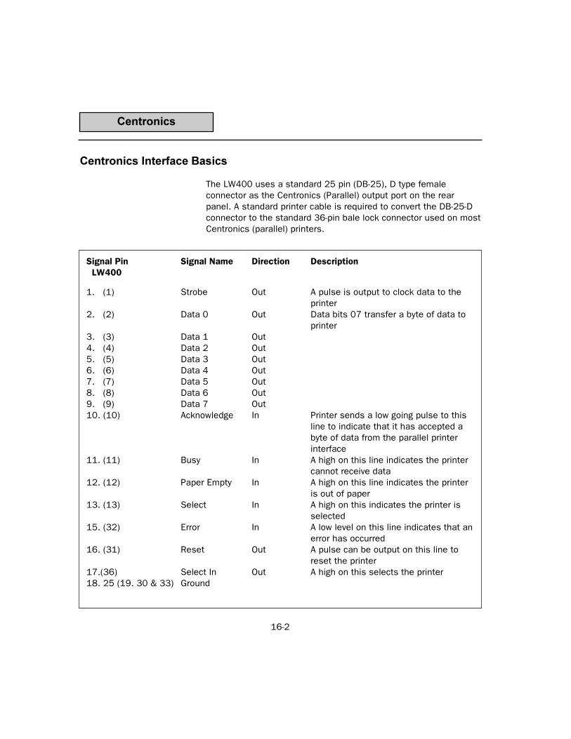
Signal Pin Signal Name Direction DescriptionLW400

1. (1) Strobe Out A pulse is output to clock data to theprinter

2. (2) Data 0 Out Data bits 07 transfer a byte of data toprinter

3. (3) Data 1 Out4. (4) Data 2 Out5. (5) Data 3 Out6. (6) Data 4 Out7. (7) Data 5 Out8. (8) Data 6 Out9. (9) Data 7 Out10. (10) Acknowledge In Printer sends a low going pulse to this

line to indicate that it has accepted abyte of data from the parallel printerinterface

11. (11) Busy In A high on this line indicates the printercannot receive data

12. (12) Paper Empty In A high on this line indicates the printeris out of paper

13. (13) Select In A high on this indicates the printer isselected

15. (32) Error In A low level on this line indicates that anerror has occurred

16. (31) Reset Out A pulse can be output on this line toreset the printer

17.(36) Select In Out A high on this selects the printer18. 25 (19. 30 & 33) Ground

16-2

Centronics

Centronics Interface Basics

The LW400 uses a standard 25 pin (DB-25), D type femaleconnector as the Centronics (Parallel) output port on the rearpanel. A standard printer cable is required to convert the DB-25-Dconnector to the standard 36-pin bale lock connector used on mostCentronics (parallel) printers.

16-3

GPIB

GPIB I/O Basics

The devices on the GPIB network may be connected in any combi-nation of a STAR or LINEAR arrangements. Standard IEEE 488.2cables must be used to connect all the devices and total lengthmust not exceed 20 meters. The devices must conform to theserules:

1. At least half the devices on the network must be turned on.

2. One network can connect no more than 15 devices (includingthe controller).

3. One device must be connected for every two meters of cable,assuming one device presents one standard device load.

4. Each device must have a unique bus address.

The LW400 communicates across the GPIB as a Talker or aListener to receive remote host commands and send responses.The LW400 implements the IEEE 488.2 interface standard asdefined by the table on the following page.

16-4

GPIB

The GPIB SETUP softkey menu is obtained by:

1. Pressing the PROJECT key.

2. Pressing the PREFERENCE key

3. Pressing the SYSTEM key

4. Pressing the GPIB key.

Address selection is the only setup parameter. Addresses from 1to 30 may be selected. 1 is the default address setting.

17-1

THE FUNCTION GENERATOR

Besides being an Arbitrary Waveform Generator, the WaveStation isalso a standard function generator. WaveStation is capable ofgenerating most standard functions such as sines, squares etc.and also some rather nonstandard functions such as multitonesand sweeps.

Activating the Standard Function Generator The Standard Function Generator is activated by pressing 2nd

followed by either the channel 1 or channel 2 select key. The func-tion generator menu is used in a manner that is the same as allother menus in the WaveStation. Pressing the Functions softkeywill cause the rotary knob to attach to that key making it possibleto dial through the list of available standard functions. Alternatelya second push of the Functions softkey will present a list of avail-able standard functions to choose from. The tables belowsummarize the available standard functions and the ranges of theparameters that are selectable by the user.

17

Figure 17.1 Selecting the Standard Function

17-2

Function Generator

Variable Range Resolution Default ValueAmplitude (peak to peak) 1 mv - 10 Volts 1 mv 1 voltBase + 5V to -5V 1 mv 0 voltsFrequency 1 Hz to 50 MHz 1 Hz 10 MHzSweep Start Frequency 1 Hz to 50 MHz 1 Hz 1 MHzSweep Stop Frequency 1 Hz to 50 MHz 1 Hz 10 MHzSweep Time 1 ns to 1 sec 1 ns 2 msSweep Type linear/natural log .LinearTime Delay 0 ns to memory length 1ns 5 nsEdge Time (risetime and falltime) 5 nsec to 500 ns 1 ns 5ns

Table 17.3 Square Wave Function Generator

Variable Range Resolution Default ValueAmplitude (peak to peak) 1 mv - 10 Volts 1 mv 1 voltOffset @ zero phase + 5V to -5V 1 mv 0 voltsFrequency 1 Hz to 100 MHz 1 Hz 10 MHzSweep Start Frequency 1 Hz to 100 MHz 1 Hz 1 MHzSweepStop Frequency 1 Hz to 100 MHz 1 Hz 10 MHzSweep Time 1 ns to 1 sec 1 ns 2 msSweep Type Linear/Natural Log .LinearStart Phase 0 to 360 .05 degree 0 degrees

Variable Range Resolution Default ValueAmplitude (peak to peak) 1 mv - 10 Volts 1 mv 1 voltOffset @ zero phase + 5V to -5V 1 mv 0 voltsFrequency 1 Hz to 25 MHz 1 Hz 10 MHzSweep Start Frequency 1 Hz to 25 MHz 1 Hz 1 MHzSweepStop Frequency 1 Hz to 25 MHz 1 Hz 10 MHzSweep Time 1 ns to 1 sec 1 ns 2 msSweep Type Linear/Natural Log .LinearStart Phase 0 to 360 .05 degree 0 degrees

Table 17.1 Sine Wave Function Generator

Table 17.2 Triangle Wave Function Generator

17-3

Function Generator

Variable Range Resolution Default ValueAmplitude (peak to peak) 1 mv - 10 Volts 1 mv 1 voltBase + 5V to -5V 1 mv 0 voltsPeriod 20 ns to memory length .1 ns 200 nsWidth 5 ns to mem length 0.1 ns 50 nsTime Delay 0 to memory length 0.1ns 0Edge Time (risetime and falltime) 5 ns to 5 ms 1 ns 10

Variable Range Resolution Default ValueAmplitude (peak to peak) 1 mv - 10 Volts 1 mv 1 voltOffset @ zero phase + 5V to -5V 1 mv 0 voltsFrequency 1 Hz to 100 MHz 1 Hz 10 MHzNumber Of Tones 1 to 10 1 Tone 1Relative Amplitude 0 to 1 .001 1 volt

Variable Range Resolution Default ValueLevel + - 5 volts 1 mv 1 volt

Variable Range Resolution Default ValueAmplitude (peak to peak) 1 mv - 10 Volts 1 mv 1 voltOffset @ zero phase + 5V to -5V 1 mv 0 voltsFrequency 1 Hz to 25 MHz 1 Hz 10 MHzSweep Start Frequency 1 Hz to 25 MHz 1 Hz 1 MHzSweep Stop Frequency 1 Hz to 25 MHz 1 Hz 10 MHzSweep Time 1 ns to 1 sec 1 ns 2 msSweep Type Linear/Natural Log .LinearStart Position 0 to 100 % .001% 0Invert on/off off

Table 17.4 Ramp Wave Function Generator

Table 17.5 Pulse Wave Function Generator

Table 17.6 Multitione Wave Function Generator

Table 17.7 DC Wave Function Generator

18-1

DISK UTILITIES

Disk Utilities Two disk utility functions are available under the SAVE menuseefigure 18.1. The disk utility functions are file search and floppy diskformat. Disk Utilities are accessed by pressing theSAVE button on the front panel and then pressingthe Disk Utilities softkey.

1188

Fig. 18.1 DiskUtilitiesMenu

Floppy Disk Format The LW400 will DOS format 1.44 MByte (high density), 3.5 inchfloppy disks. Select Format Floppy from the Disk Utilities menu tobegin the formatting process. The format opera-tion is confirmed by a dialog box to preventerroneous erasure of data.

Fig. 18.2Floppy Disk

Format Menu

18-2

The result of the file search operation is a report box listing thefiles found by name, type, and project. Use Page Up and PageDown to view any additional pages.

Disk Utilities

Hard Disk File Search Utility The hard disk file search utility is controlled from

the Find File menu. File search will find wave-forms, sequences, equations, or all file types, byname, as specified in the What menu field. A wildcard character (*) may be used as a substitute fora group of characters at the beginning or end ofany file name.

Fig. 18.3 HardDisk FileSearch

Figure 18.4 File search resuts

A-1

APPENDIX AA

Figure A-1

Figure A-2

A-2

Appendix A

Measurement Functions Description

IntroductionWaveform parameters supported by the LW400 are described inthe following pages in alphabetical order. The description of eachparameter follows the form shown below. If a section is notneeded for a particular parameter, it is omitted.

Full Name Abbreviated Name

Description: This section contains a brief description of the parameter. It is intended toconvey the meaning and use of the parameter without getting into technicaldetails.

Definition: This is a more technical description of the parameter than the one given above.

Diagram: Diagrams referenced by the current parameter are given here. At the end of thesection on parameters, there is a single page containing diagrams which help toexplain the definitions of the parameters.

Restrictions: This indicates conditions necessary for the computation of the parameter.

Special Cases: This describes situations in which the parameter may be computed differentlydepending on the data in the waveform.

Units: The units of the parameter are given here.

Notes: This section describes any unusual or unexpected behavior of the parameter. Itmay indicate the differences between this and related parameters.

A-3

Appendix A

Fall Time fall

Description: Fall time measures the time between the 10% and 90% values on the fallingedges of a waveform. The FALL times of each edge between the cursors are aver-aged to produce the final result.

Definition: Time at Lower Threshold - Time at Upper Threshold averaged over all fallingedges.

Diagram: Figure A-1

Restrictions: The waveform is assumed to have two major levels. For signals in which this isnot true, such as triangle or sawtooth waves, FALL may not give results.

Units: Seconds

A-4

Appendix A

Minimum Level min

Diagram: Figure A-1

Description: MINIMUM LEVEL measures the lowest point in a waveform. MIN makes no suchassumptions that the waveform has two basic levels.

Definition: Lowest value in the waveform between the cursors.

Units: Volts

A-5

Appendix A

Maximum Level max

Description: MAXIMUM LEVEL measures the highest point in a waveform.

Definition: Highest value in the waveform between the cursors.

Diagram: Figure A-1

Units: Volts

A-6

Appendix A

Rise Time rise

Description: Rise time measures the time between the 10% and 90% values on the risingedges of a waveform. The RISE times for each rising edge on the screen orbetween the cursors is averaged to produce the final result.

Definition: Time at Upper Threshold - Time at Lower Threshold averaged over each risingedge.

Diagram: Figure A-1

Restrictions: The waveform is assumed to have two major levels. For signals in which this isnot true, such as triangle or sawtooth waves, RISE may not give predictableresults.

Units: Seconds

A-7

Apendix A

Width Positive widp

Description: The width of a cyclic signal is determined by examining 50% cross-ings in the input data. WIDTH POSITIVE searches for a rising edgeafter the left edge or left cursor. In this case, WIDTH is the timebetween adjacent rising and falling edges.

The widths of all pulses in the waveform are averaged to producethe final result.

Definition: Width of the first positive pulse, averaged for all similar pulses.

Diagram: Figures A-1 and A-2

Units: Seconds.

A-8

Appendix A

Period per

Description: The period of a cyclic signal is measured as the time betweenevery other pair of 50% crossings. Beginning with the first transi-tion defined by the left edge of the graticule or, the left cursor, theperiod is measured for each pair of transitions. These values areaveraged to produce the final result.

Definition: Time between odd numbered 50% crossings beginning with the leftmost crossing between the cursors, averaged over all such pairs ofcrossings.

Diagram: Figures A-2

Units: Seconds.

B-1

APPENDIX B

LW400/LW400A/LW400B WaveStation Specifications

Generator Mode Standard Function Waveforms - 1 Hz ResolutionSine, 1 Hz - 100 MHzSquare, 1 Hz - 50 MHzTriangle, 1 Hz - 25 MHzRamp, 1 Hz - 25 MHzPulse, (period)20 ns - max. memory DC

Frequency Sweep Linear / LogMultitone, 1-10 tones, 1 Hz - 100 MHz

Arbitrary Functions: Waveform CreationInteractive Graphical editor on Internal 9 CRT

Standard FunctionsSine, Square, Triangle, Ramp, Pulse, DC

Equation EditorWaveform (array) MathWaveform Import From

Digital OscilloscopeFloppy Disk

Waveform Feature Time Resolution: 100 ps

Available memory: 256k/ch. standard, 1 Mpoint optional

Minimum segment length:64 points

Maximum segment length: Up to available memory (1Mpoint when optional memoryinstalled)

Segment length resolution: 1 point

Number of links: 512 for 256k memory2048 for 1M memory

Internal Noise Generator: Available in LW400 and LW400A onlyIndependent pseudorandom white noise generator with Gaussiandistribution and 222 states

B-2

Appendix B

Waveform Output Output channels: Characteristics LW410/LW410A - 1 Channel

LW420/LW420A - 2 ChannelOutput Impedance:

50 Ω , ± 5%DC Accuracy:

±(2% of setting +40 mV) for output > 500 mV peak-peak±(2% of setting +15 mV) for output ≤ 500 mV peak-peak

Vertical resolution: 8 bits

Minimum output voltage: 10 mV p-p into 50 Ω

Maximum output voltage: 10 V p-p into 50 Ω

Offset voltage range: ± 5 V into 50 Ω. The output voltage (signal + offset) must bein the range ± 5 V into 50 Ω .

Offset voltage resolution: 0.05% of full scale

Output bandwidth: 100 MHz (-3dB) (widest bandwidth)

Total harmonic distortion: <5 V p-p <-45 dBc (-50 dBc typical)

for sinusoidal output <=1MHz <-35dBC

for sinusoidal output 1 MHz to 20 MHz (<-45 dBc typical) <-25 dBc

to 50 MHz (<-40 dBc typical) (predominantly 2nd harmonic)Spurious & non-harmonic distortion:

<-60 dBc for frequencies <=1 MHz for outputSignal-to-noise ratio:

>40 dB (-45 typical) for output amplitudes >100 mV @ 0 offsetTransition times: @ widest bandwidth with band limiting off

LW400/LW400A/LW400B: < 6 ns 10%- 90% LW400/LW400A/LW400B: < 5 ns 10%- 90% @ widest

bandwidth with band limiting offOvershoot and ringing:

<8% of step size max. 3% typicalSettling time:

<50 ns to within 3% of step size @ widest bandwidthInter-channel crosstalk: <1%Squarewave Symmetry: < 6 ppm + 0.5 ns

B-3

Appendix B

Pulse Generator Characteristics: Pulse repetition frequency(max): 50 MHzPulse repetition frequency(min):

Limited by Channel memory and clock speedFrequency accuracy: ± 3 ppm over operating temperaturerangePulse width(max): Limited by channel memory and clock speedPulse width(min): 10 nsPulse width accuracy:

± 3 ppm + 0.5 ns for widths > 2x the risetimePulse delay Characteristics:

Same as trigger delay with the following exception. pulse time delay resolution = 1 ns

Ch 1 to Ch 2 skew: <1 ns for identical waveforms in each channel (widest bw)

Output protection: ± 20 V

Output filtering: The following filter cutoff frequencies will be available; 100 MHz Gaussian, 10 MHz Gaussian, 1 MHz Gaussian, 100kHz Gaussian, 10 kHz Gaussian

Sample clock characteristics: (with internal 10 MHz reference)Maximum sample rate:

400 MS/secondAccuracy:

±3 ppm over operating temperature rangeStability:

Aging <1 ppm/yearSSB Phase Noise:

LW410/LW420: <-95 (-100 typical) dBc/Hz @ 10 KHz offset for a 10 MHz sine wave at output

LW410A/LW420A: <-90 dBc/Hz @ 10 KHz offset for a 10 MHz sine wave at output

Resolution: 1 Hz

Variable Clock LW400A and LW400B series onlyVariable over range of 6 Khz to 400 MHz

Triggering Characteristics Trigger slope: Positive or NegativeTrigger input impedance: 50 Ω ± 5%Threshold range: ± 2.5VThreshold resolution: 20 mVThreshold accuracy: ±100 mV Threshold sensitivity: 50 mV minimum p-pMinimum pulse width: ≤ 5 ns

Protection: ± 5 V

Trigger ModesContinuous:

Runs continuouslySingle:

Outputs 1 repetition of the waveform for each trigger received.Triggers received while the waveform is still running areignored.

Burst: Outputs the selected waveform a programmable number oftimes in response to a trigger. The maximum number of repeti-tions for a burst is 4,096. Triggers received while the burst isrunning are ignored.

Gated: The waveform starts on the leading edge of the gate signal andstops on completion of the waveform cycle occuring at thetrailing edge of the gate signal.

B-4

Appendix B

B-5

Appendix B

Trigger DelayMinimum(min) delay time:

35 ns ±3.5 ns +5 sample clocksMaximum delay time:

(232-1) sample clocksDelay resolution:

1 sample clock. The delay will be programmed in units ofseconds. When operating from the front panel the resolution(sample clock period) will be shown to the user and the delaywill change in increments of that value.

Delay accuracy: ± (0.0003% x programmed value)+min delay time+delay jitter

Note: The min delay time is a fixed value for each instrumentat the selected sample clock rate. Considering this fact, thetime delay at a specific sample clock rate can be measuredand used to offset the programmed value to obtain the desiredtime delay.

offset programmed value = desired value - measured delay

In this case the delay accuracy is: ± (0.0003% x offset programmed value)+delay jitter

Delay jitter: 1 sample clock

Trigger SourcesManual:

Front panel pushbuttonExternal:

Front panel BNC connectorGPIB:

A trigger command may be issued over the GPIB bus

B-6

Appendix B

Auxiliary Inputs External 10 MHz reference: A rear panel input is provided thatallows an external reference clock to be input. 400 mV p-p to 5 Vp-p into 50 Ω.

Noise Input: ±500 mV maximum into 50 Ω.

Auxiliary Outputs 10 MHz reference output:Frequency accuracy: ± 3 ppmAmplitude (high): ≥ 1.6 v into 50 ΩAmplitude (low): ≤ 0.2 v into 50 Ω

Timing marker:1 bit of memory up to 128 transitions definableOutput levels:

ECL or TTL levelsProtection:

Outputs are protected to ± 5 V

Digital Output: Channel 1 only, 8 bits and clock available from rear panel.TTL/ECL logic levels simultaneously.

Noise In/Out: From rear panel BNC Connectors

Hard Copy Outputs Supported Printers include:Epson MX/FXEpson LQHP LaserJet IIHP ThinkJet

Programmability GPIB IEEE 488.2 compatible. Compliant with SCPI programminglanguage. Capable of initiating and controlling waveform transferfrom digital oscilloscopes by simply connecting a GPIB cable (nocomputer required).

B-7

Appendix B

General Temperature: 5° C to 35° C full specifications; 0° C to 40° C operating;-20° C to 70° C non-operating.

Humidity:10% to 80% relative, non-condensing

Altitude:< 2000 Meters (6560 ft)

Power:90 - 132/180-250 V AC47 - 63 Hz4 amps @ 115 V AC (20 amps cold start surge)2 amps @ 230 V AC (40 amps cold start surge)

The power supply is internally protected against short circuitand overload by means of a single T5.0A/250 V ~ fuse,which is not replaceable by the user.

Dimensions (HWD):7.67, 14.92, 19.58 (inches)19.5, 37.9, 49.7 (cm)

Weight: 27.6 lbs (12.5 kilograms)

Warranty: One year

Calibration Interval: Annually

B-8

Appendix B

CE Certifications: CE, UL and cUL

The Wavestation meets requirements of the EMC Directive89/336/EEC for Electromagnetic Compatibility and Low VoltageDirective 73/23/EEC for Product Safety. See "Declaration ofConformity" certificate for details.

Warning: This is a Class A product. In a domestic environmentthis product may cause radio interference, in which case the usermay be required to take adequate measures.

UL and cUL Certifcations:

UL Standard: UL 3111-1

Canadian Standard: CSA-C22.2 No. 1010.1-92

TABLE OF CONTENTS - Teledyne LeCroycdn.teledynelecroy.com/files/manuals/lw400a-om2.pdfCAUTION: Refer...

Documents

Transcript of TABLE OF CONTENTS - Teledyne LeCroycdn.teledynelecroy.com/files/manuals/lw400a-om2.pdfCAUTION: Refer...