Table of Contents Chapter 6 (Network Optimization Problems)aa2035/CourseBase/Oper… · PPT...
36
Table of Contents Chapter 6 (Network Optimization Problems) Minimum-Cost Flow Problems (Section 6.1) 6.2–6.12 A Case Study: The BMZ Maximum Flow Problem (Section 6.2) 6.13–6.16 Maximum Flow Problems (Section 6.3) 6.17–6.21 Shortest Path Problems: Littletown Fire Department (Section 6.4) 6.22–6.25 Shortest Path Problems: General Characteristics (Section 6.4) 6.26–6.27 Shortest Path Problems: Minimizing Sarah’s Total Cost (Section 6.4) 6.28–6.31 Shortest Path Problems: Minimizing Quick’s Total Time (Section 6.4) 6.32–6.36 © 2014 by McGraw-Hill Education. This is proprietary material solely for authorized instructor use. Not authorized for sale or distribution in any manner. This document may not be copied, scanned, duplicated, forwarded, distributed, or posted on a website, in whole or part.
Transcript of Table of Contents Chapter 6 (Network Optimization Problems)aa2035/CourseBase/Oper… · PPT...

Table of ContentsChapter 6 (Network Optimization Problems)
Minimum-Cost Flow Problems (Section 6.1) 6.2–6.12A Case Study: The BMZ Maximum Flow Problem (Section 6.2) 6.13–6.16Maximum Flow Problems (Section 6.3) 6.17–6.21Shortest Path Problems: Littletown Fire Department (Section 6.4) 6.22–6.25Shortest Path Problems: General Characteristics (Section 6.4) 6.26–6.27Shortest Path Problems: Minimizing Sarah’s Total Cost (Section 6.4) 6.28–6.31Shortest Path Problems: Minimizing Quick’s Total Time (Section 6.4) 6.32–6.36
© 2014 by McGraw-Hill Education. This is proprietary material solely for authorized instructor use. Not authorized for sale or distribution in any manner. This document may not be copied, scanned, duplicated, forwarded, distributed, or posted on a website, in whole or part.

Distribution Unlimited Co. Problem
• The Distribution Unlimited Co. has two factories producing a product that needs to be shipped to two warehouses– Factory 1 produces 80 units.– Factory 2 produces 70 units.– Warehouse 1 needs 60 units.– Warehouse 2 needs 90 units.
• There are rail links directly from Factory 1 to Warehouse 1 and Factory 2 to Warehouse 2.
• Independent truckers are available to ship up to 50 units from each factory to the distribution center, and then 50 units from the distribution center to each warehouse.
Question: How many units (truckloads) should be shipped along each shipping lane?
6-2

The Distribution Network
F1
DC
F2 W2
W180 unitsproduced
70 units produced
60 unitsneeded
90 units needed
6-3

Data for Distribution Network
F1
DC
F2 W2
W180 unitsproduced
70 units produced
60 unitsneeded
90 units needed
$700/unit
$1,000/unit
$300/unit
[50 units max.]
$500/unit
[50 units max.]
$200/unit
[50 units max.]
$400/unit [50 units max.]
6-4

A Network Model
F1
DC
F2 W2
W1$700
$1,000
[80] [- 60]
[- 90][70]
[0]$300 [50]
$200 [50]
$500 [50]
$400 [50]
6-5

The Optimal Solution
F1
DC
F2 W2
W1(30)
(40)
[80] [- 60]
[- 90][70]
[0](50)
(30)
(30)
(50)
6-6

Terminology for Minimum-Cost Flow Problems
1. The model for any minimum-cost flow problem is represented by a network with flow passing through it.
2. The circles in the network are called nodes.
3. Each node where the net amount of flow generated (outflow minus inflow) is a fixed positive number is a supply node.
4. Each node where the net amount of flow generated is a fixed negative number is a demand node.
5. Any node where the net amount of flow generated is fixed at zero is a transshipment node. Having the amount of flow out of the node equal the amount of flow into the node is referred to as conservation of flow.
6. The arrows in the network are called arcs.
7. The maximum amount of flow allowed through an arc is referred to as the capacity of that arc.
6-7

Assumptions of a Minimum-Cost Flow Problem
1. At least one of the nodes is a supply node.
2. At least one of the other nodes is a demand node.
3. All the remaining nodes are transshipment nodes.
4. Flow through an arc is only allowed in the direction indicated by the arrowhead, where the maximum amount of flow is given by the capacity of that arc. (If flow can occur in both directions, this would be represented by a pair of arcs pointing in opposite directions.)
5. The network has enough arcs with sufficient capacity to enable all the flow generated at the supply nodes to reach all the demand nodes.
6. The cost of the flow through each arc is proportional to the amount of that flow, where the cost per unit flow is known.
7. The objective is to minimize the total cost of sending the available supply through the network to satisfy the given demand. (An alternative objective is to maximize the total profit from doing this.)
6-8

Properties of Minimum-Cost Flow Problems
• The Feasible Solutions Property: Under the previous assumptions, a minimum-cost flow problem will have feasible solutions if and only if the sum of the supplies from its supply nodes equals the sum of the demands at its demand nodes.
• The Integer Solutions Property: As long as all the supplies, demands, and arc capacities have integer values, any minimum-cost flow problem with feasible solutions is guaranteed to have an optimal solution with integer values for all its flow quantities.
6-9

Spreadsheet Model
3456789
1011
B C D E F G H I J K LFrom To Ship Capacity Unit Cost Nodes Net Flow Supply/Demand
F1 W1 30 $700 F1 80 = 80F1 DC 50 <= 50 $300 F2 70 = 70DC W1 30 <= 50 $200 DC 0 = 0DC W2 50 <= 50 $400 W1 -60 = -60F2 DC 30 <= 50 $400 W2 -90 = -90F2 W2 40 $900
Total Cost $110,000
345678
JNet Flow
=SUMIF(From,I4,Ship)-SUMIF(To,I4,Ship)=SUMIF(From,I5,Ship)-SUMIF(To,I5,Ship)=SUMIF(From,I6,Ship)-SUMIF(To,I6,Ship)=SUMIF(From,I7,Ship)-SUMIF(To,I7,Ship)=SUMIF(From,I8,Ship)-SUMIF(To,I8,Ship)
6-10

The SUMIF Function
• The SUMIF formula can be used to simplify the node flow constraints.
=SUMIF(Range A, x, Range B)
• For each quantity in (Range A) that equals x, SUMIF sums the corresponding entries in (Range B).
• The net outflow (flow out – flow in) from node x is then
=SUMIF(“From labels”, x, “Flow”) – SUMIF(“To labels”, x, “Flow”)
6-11

Typical Applications of Minimum-Cost Flow Problems
Kind ofApplication
SupplyNodes
Transshipment Nodes
DemandNodes
Operation of a distribution network Sources of goods Intermediate storage
facilities Customers
Solid waste management
Sources of solid waste Processing facilities Landfill locations
Operation of a supply network Vendors Intermediate
warehouses Processing facilities
Coordinating product mixes at plants Plants Production of a
specific productMarket for a specific product
Cash flow management
Sources of cash at a specific time
Short-term investment options
Needs for cash at a specific time
6-12

The BMZ Maximum Flow Problem
• The BMZ Company is a European manufacturer of luxury automobiles. Its exports to the United States are particularly important.
• BMZ cars are becoming especially popular in California, so it is particularly important to keep the Los Angeles center well supplied with replacement parts for repairing these cars.
• BMZ needs to execute a plan quickly for shipping as much as possible from the main factory in Stuttgart, Germany to the distribution center in Los Angeles over the next month.
• The limiting factor on how much can be shipped is the limited capacity of the company’s distribution network.
Question: How many units should be sent through each shipping lane to maximize the total units flowing from Stuttgart to Los Angeles?
6-13

The BMZ Distribution Network
ST
LI
BO
RO
NO
NY
LA
New York
Rotterdam
Stuttgart
LisbonNew Orleans
{40 units max.]
Bordeaux[70 units max.]
Los Angeles
[80 units max.]
[60 units max.]
[50 units max.]
[30 units max.]
[50 units max.]
[40 units max.]
[70 units max]
6-14

A Network Model for BMZ
ST
LI
BO
RO
NO
NY
LA[70]
[80]
[70]
[60]
[40]
[50]
[30]
[50]
[40]
6-15
Spreadsheet Model for BMZ
3456789
1011121314
B C D E F G H I J KFrom To Ship Capacity Nodes Net Flow Supply/Demand
Stuttgart Rotterdam 50 <= 50 Stuttgart 150Stuttgart Bordeaux 70 <= 70 Rotterdam 0 = 0Stuttgart Lisbon 30 <= 40 Bordeaux 0 = 0
Rotterdam New York 50 <= 60 Lisbon 0 = 0Bordeaux New York 30 <= 40 New York 0 = 0Bordeaux New Orleans 40 <= 50 New Orleans 0 = 0
Lisbon New Orleans 30 <= 30 Los Angeles -150New York Los Angeles 80 <= 80
New Orleans Los Angeles 70 <= 70
Maximum Flow 150
6-16

Assumptions of Maximum Flow Problems
1. All flow through the network originates at one node, called the source, and terminates at one other node, called the sink. (The source and sink in the BMZ problem are the factory and the distribution center, respectively.)
2. All the remaining nodes are transshipment nodes.
3. Flow through an arc is only allowed in the direction indicated by the arrowhead, where the maximum amount of flow is given by the capacity of that arc. At the source, all arcs point away from the node. At the sink, all arcs point into the node.
4. The objective is to maximize the total amount of flow from the source to the sink. This amount is measured in either of two equivalent ways, namely, either the amount leaving the source or the amount entering the sink.
6-17

BMZ with Multiple Supply and Demand Points
• BMZ has a second, smaller factory in Berlin.
• The distribution center in Seattle has the capability of supplying parts to the customers of the distribution center in Los Angeles when shortages occur at the latter center.
Question: How many units should be sent through each shipping lane to maximize the total units flowing from Stuttgart and Berlin to Los Angeles and Seattle?
6-18

Network Model for The Expanded BMZ Problem
ST
BE
BO
NY
LI
NO
HA
BN
RO
LA
SE
[70]
[20]
[20]
[40]
[10]
[80]
[70]
[40]
[30]
[60]
[40]
[50]
[30]
[60]
[50]
[40]
6-19

Spreadsheet Model
3456789
101112131415161718192021
B C D E F G H I J KFrom To Ship Capacity Nodes Net Flow Supply/Demand
Stuttgart Rotterdam 40 <= 50 Stuttgart 140Stuttgart Bordeaux 70 <= 70 Berlin 80Stuttgart Lisbon 30 <= 40 Hamburg 0 = 0
Berlin Rotterdam 20 <= 20 Rotterdam 0 = 0Berlin Hamburg 60 <= 60 Bordeaux 0 = 0
Rotterdam New York 60 <= 60 Lisbon 0 = 0Bordeaux New York 30 <= 40 Boston 0 = 0Bordeaux New Orleans 40 <= 50 New York 0 = 0
Lisbon New Orleans 30 <= 30 New Orleans 0 = 0Hamburg New York 30 <= 30 Los Angeles -160Hamburg Boston 30 <= 40 Seattle -60
New Orleans Los Angeles 70 <= 70New York Los Angeles 80 <= 80New York Seattle 40 <= 40
Boston Los Angeles 10 <= 10Boston Seattle 20 <= 20
Maximum Flow 220
6-20

Some Applications of Maximum Flow Problems
1. Maximize the flow through a distribution network, as for BMZ.
2. Maximize the flow through a company’s supply network from its vendors to its processing facilities.
3. Maximize the flow of oil through a system of pipelines.
4. Maximize the flow of water through a system of aqueducts.
5. Maximize the flow of vehicles through a transportation network.
6-21

Littletown Fire Department
• Littletown is a small town in a rural area.
• Its fire department serves a relatively large geographical area that includes many farming communities.
• Since there are numerous roads throughout the area, many possible routes may be available for traveling to any given farming community.
Question: Which route from the fire station to a certain farming community minimizes the total number of miles?
6-22

The Littletown Road System
Fire Station
H
G
F
E
D
C
B
A
36
42
1
7
5
4
6
8
6
4
3
4
6
7
52
3
Farming Community
6-23

The Network Representation
T
H
G
F
E
D
B
C
A
O (Destination)(Origin)
3
6
1
2
6
4
34
7
8
6
5
42
34
6
75
6-24

Spreadsheet Model
34567891011121314151617181920212223242526272829
B C D E F G H I J KFrom To On Route Distance Nodes Net Flow Supply/Demand
Fire St. A 1 3 Fire St. 1 = 1Fire St. B 0 6 A 0 = 0Fire St. C 0 4 B 0 = 0
A B 1 1 C 0 = 0A D 0 6 D 0 = 0B A 0 1 E 0 = 0B C 0 2 F 0 = 0B D 0 4 G 0 = 0B E 1 5 H 0 = 0C B 0 2 Farm Com. -1 = -1C E 0 7D E 0 3D F 0 8E D 0 3E F 1 6E G 0 5E H 0 4F G 0 3F Farm Com. 1 4G F 0 3G H 0 2G Farm Com. 0 6H G 0 2H Farm Com. 0 7
Total Distance 19
6-25

Assumptions of a Shortest Path Problem
1. You need to choose a path through the network that starts at a certain node, called the origin, and ends at another certain node, called the destination.
2. The lines connecting certain pairs of nodes commonly are links (which allow travel in either direction), although arcs (which only permit travel in one direction) also are allowed.
3. Associated with each link (or arc) is a nonnegative number called its length. (Be aware that the drawing of each link in the network typically makes no effort to show its true length other than giving the correct number next to the link.)
4. The objective is to find the shortest path (the path with the minimum total length) from the origin to the destination.
6-26

Applications of Shortest Path Problems
1. Minimize the total distance traveled.
2. Minimize the total cost of a sequence of activities.
3. Minimize the total time of a sequence of activities.
6-27

Minimizing Total Cost: Sarah’s Car Fund
• Sarah has just graduated from high school.
• As a graduation present, her parents have given her a car fund of $21,000 to help purchase and maintain a three-year-old used car for college.
• Since operating and maintenance costs go up rapidly as the car ages, Sarah may trade in her car on another three-year-old car one or more times during the next three summers if it will minimize her total net cost. (At the end of the four years of college, her parents will trade in the current used car on a new car for Sarah.)
Question: When should Sarah trade in her car (if at all) during the next three summers?
6-28

Sarah’s Cost Data
Operating and Maintenance Costsfor Ownership Year
Trade-in Value at Endof Ownership Year
PurchasePrice 1 2 3 4 1 2 3 4
$12,000 $2,000 $3,000 $4,500 $6,500 $8,500 $6,500 $4,500 $3,000
6-29

Shortest Path Formulation
(Origin) (Destination)4321
17,00010,500
10,500
5,500 5,500 5,500 5,500
25,000
17,000
10,500
0
6-30

Spreadsheet Model
34567891011121314151617181920212223
B C D E F G H I JOperating & Trade-in Value PurchaseMaint. Cost at End of Year Price
Year 1 $2,000 $8,500 $12,000Year 2 $3,000 $6,500Year 3 $4,500 $4,500Year 4 $6,500 $3,000
From To On Route Cost Nodes Net Flow Supply/DemandYear 0 Year 1 0 $5,500 Year 0 1 = 1Year 0 Year 2 1 $10,500 Year 1 0 = 0Year 0 Year 3 0 $17,000 Year 2 0 = 0Year 0 Year 4 0 $25,000 Year 3 0 = 0Year 1 Year 2 0 $5,500 Year 4 -1 = -1Year 1 Year 3 0 $10,500Year 1 Year 4 0 $17,000Year 2 Year 3 0 $5,500Year 2 Year 4 1 $10,500Year 3 Year 4 0 $5,500
Total Cost $21,000
6-31
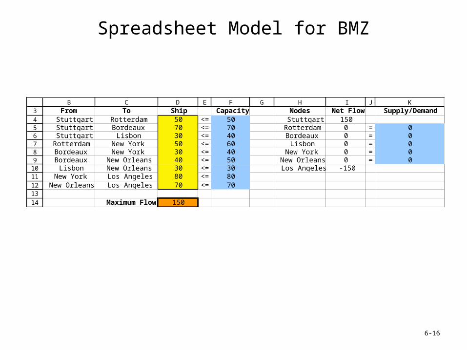
Minimizing Total Time: Quick Company
• The Quick Company has learned that a competitor is planning to come out with a new kind of product with great sales potential.
• Quick has been working on a similar product that had been scheduled to come to market in 20 months.
• Quick’s management wishes to rush the product out to meet the competition.
• Each of four remaining phases can be conducted at a normal pace, at a priority pace, or at crash level to expedite completion. However, the normal pace has been ruled out as too slow for the last three phases.
• $30 million is available for all four phases.
Question: At what pace should each of the four phases be conducted?
6-32

Time and Cost of the Four Phases
LevelRemainingResearch Development
Design ofMfg. System
Initiate Productionand Distribution
Normal 5 months — — —
Priority 4 months 3 months 5 months 2 months
Crash 2 months 2 months 3 months 1 month
LevelRemainingResearch Development
Design ofMfg. System
Initiate Productionand Distribution
Normal $3 million — — —
Priority 6 million $6 million $9 million $3 million
Crash 9 million 9 million 12 million 6 million
6-33

Shortest Path Formulation
(Norm
al)
(Crash)
(Crash)
(Priority
) (Crash)
(Crash)
(Crash)
(Priority)
(Crash)
(Crash)
(Crash)
(Crash)5
3
3
2
3 1
132
(Priority
)
(Crash)1
2
3
3
2
,
T
3, 6
3, 9
3, 12
2, 12
2, 15
2, 18
2, 21
1, 21
1, 240, 30
1, 27
3, 3
4, 9
4, 6
4, 3
4, 0
(Origin) (Destination)(Norm
al)
(Priority)(Crash)
(Crash)
(Priority
)
(Priority) (Priority)
(Crash)
(Crash)
(Crash)
(Priority) (Priority) (Priority)
(Crash)
(Crash)
(Crash)
(Priority) ((Priority)
(Crash)5
35 2
0
0
0
0
25
3
42
3 (Priority) (Priority)5
1
132
(Priority
)
(Crash)2
1
2
3
3
2
5
2
6-34

Spreadsheet Model
From To On Route Time Nodes Net Flow Supply/Demand(0, 30) (1, 27) 0 5 (0, 30) 1 = 1(0, 30) (1, 24) 0 4 (1, 27) 0 = 0(0, 30) (1, 21) 1 2 (1, 24) 0 = 0(1, 27) (2, 21) 0 3 (1, 21) 0 = 0(1, 27) (2, 18) 0 2 (2, 21) 0 = 0(1, 24) (2, 18) 0 3 (2, 18) 0 = 0(1, 24) (2, 15) 0 2 (2, 15) 0 = 0(1, 21) (2, 15) 1 3 (2, 12) 0 = 0(1, 21) (2, 12) 0 2 (3, 12) 0 = 0(2, 21) (3, 12) 0 5 (3, 9) 0 = 0(2, 21) (3, 9) 0 3 (3, 6) 0 = 0(2, 18) (3, 9) 0 5 (3, 3) 0 = 0(2, 18) (3, 6) 0 3 (4, 9) 0 = 0(2, 15) (3, 6) 0 5 (4, 6) 0 = 0(2, 15) (3, 3) 1 3 (4, 3) 0 = 0(2, 12) (3, 3) 0 5 (4, 0) 0 = 0(3, 12) (4, 9) 0 2 (T) -1 = -1(3, 12) (4, 6) 0 1(3, 9) (4, 6) 0 2(3, 9) (4, 3) 0 1(3, 6) (4, 3) 0 2(3, 6) (4, 0) 0 1(3, 3) (4, 0) 1 2(4, 9) (T) 0 0(4, 6) (T) 0 0(4, 3) (T) 0 0(4, 0) (T) 1 0
Total Time 10
6-35

The Optimal Solution
Phase Level Time Cost
Remaining research Crash 2 months $9 million
Development Priority 3 months 6 million
Design of manufacturing system Crash 3 months 12 million
Initiate production and distribution Priority 2 months 3 million
Total 10 months $30 million
6-36