ARC HYDRO GROUNDWATER TUTORIALS - Aquaveo - Water Modeling Solutions

UTEXAS4
A COMPUTER PROGRAM FOR SLOPE STABILITY CALCULATIONS
By
Stephen G. Wright
May 1999 - Revised September 1999
Shinoak Software Austin, Texas
Copyright © 1999, 2007 by Stephen G. Wright - All Rights Reserved

i
TABLE OF CONTENTS Page
LIST OF TABLES................................................................................................................ viii
LIST OF FIGURES ............................................................................................................... xii
Section 1. INTRODUCTION ............................................................................................... 1
Section 2. RUNNING UTEXAS4 ....................................................................................... 3 Introduction .................................................................................................................. 3 Running UTEXAS4 ..................................................................................................... 3 Printing Output ............................................................................................................. 3 UTEXAS4 Application Settings .................................................................................. 4
Miscellaneous .................................................................................................. 4 Type of Units ....................................................................................... 4 Input File Path Name ........................................................................... 5 Default Input File Directory ................................................................. 5 Wide Format for Output ....................................................................... 5 Output Font for Text ............................................................................ 5 Output Font for Page Numbers ............................................................ 6 Attempt to Switch Point Sequence ...................................................... 6 Delete Duplicate Points ........................................................................ 6 Save Settings ........................................................................................ 6 Constants .......................................................................................................... 6 Maximum Number of Slices ................................................................ 7 Unit Weight of Water ........................................................................... 7 Default Force and Moment Imbalances ............................................... 7 Default Minimum Weight .................................................................... 7 Maximum Iterations ............................................................................. 8 Maximum Radius ................................................................................. 8 Decimal Places ................................................................................................. 8
Section 3. GENERAL DESCRIPTION OF INPUT DATA REQUIREMENTS ............. 13 Introduction................................................................................................................. 13 Sequence of Input ...................................................................................................... 13 Coordinate System ..................................................................................................... 14 Units for Data ............................................................................................................. 14 Default Values ........................................................................................................... 15 General Recommendations and Cautions Regarding External Water and Submerged Slopes ......................................................................................... 15 Limits on Data and Problem Size .............................................................................. 16 Compatibility with UTEXAS3 Input Data ................................................................ 16 Formats for Reading Input Data ................................................................................ 17
Blank Lines .................................................................................................... 17 Comment Lines .............................................................................................. 18
Section 4. COMMAND WORDS ...................................................................................... 20

ii
TABLE OF CONTENTS - Continued Page
Section 5. GROUP A DATA FOR HEADING AND LABELS (Optional) ...................... 24 Introduction ................................................................................................................ 24 Heading Data Input .................................................................................................... 24 Label Data Input .........................................................................................................24
Section 6. GROUP B DATA FOR PROFILE LINES ....................................................... 27 Introduction ................................................................................................................ 27 Relationship Between Profile Lines and Slope Geometry ......................................... 27 Input Data Format ..................................................................................................... 28
Section 7. GROUP C DATA FOR MATERIAL PROPERTIES ...................................... 33 Introduction................................................................................................................. 33 Effective Stress versus Total Stress Analyses ............................................................ 33 Properties for Multi-Stage Computations ................................................................... 34 Unit Weights ............................................................................................................... 34 Shear Strength Options ............................................................................................... 35
Option 1 (Conventional c, φ Strength) ........................................................... 35 Option 2 (Linear Increase below Profile Line) .............................................. 35 Option 3 (Linear Increase Below Horizontal Reference) .............................. 36 Option 4 (Constant c/ p Ratio) ....................................................................... 36 Option 5 (Anisotropic Strengths).................................................................... 37 Option 6 (Nonlinear, Curved Failure Envelope) ............................................ 37 Option 7 (Interpolation of Strength) .............................................................. 38 Option 8 (Two-Stage Strength - Linear Envelopes) ...................................... 39 Option 9 (Two-Stage Strength - Nonlinear Envelopes) ................................. 39 Option 10 ("Very High" Strengths) ............................................................... 39
Pore Water Pressure Options .......................................................................................40 Option 1 (No Pore Water Pressure) ............................................................... 40 Option 2 (Constant Pore Water Pressure) ...................................................... 40 Option 3 (Constant Pore Water Pressure Coefficient, ru) .............................. 40 Option 4 (Piezometric Line) .......................................................................... 40 Option 5 (Pressure Interpolated) .................................................................... 41 Option 6 (Pressure Coefficients, ru, Interpolated) .......................................... 41 Negative Pore Water Pressures ...................................................................... 41
Input Data Format ..................................................................................................... 41
Section 8. GROUP D DATA FOR THE PIEZOMETRIC LINE (Optional) .................... 57 Introduction ................................................................................................................ 57 Relationship between Piezometric Lines and Surface Water Loads ......................... 57 Description of Data .................................................................................................... 57 Multi-Stage Computations ......................................................................................... 58
Input Data Format ..................................................................................................... 58
iii
TABLE OF CONTENTS - Continued Page
Section 9. GROUP E DATA FOR INTERPOLATION OF PORE WATER PRESSURES AND SHEAR STRENGTHS (Optional) ................................... 62
Introduction ................................................................................................................ 62 Interpolation Scheme ................................................................................................. 62 Input Data Format .................................................................................................... 64
Section 10. GROUP F DATA FOR THE SLOPE GEOMETRY (Optional) ...................... 73 Introduction................................................................................................................. 73 Description of Data ..................................................................................................... 73 Special Note for Flat Slopes ....................................................................................... 74 Input Data Format ...................................................................................................... 74
Section 11. GROUP G DATA FOR DISTRIBUTED LOADS (Optional) ......................... 76 Introduction ................................................................................................................ 76 Description of Data .................................................................................................... 76 Automatic Generation of Distributed Load Data ....................................................... 77 Multi-Stage Computations ......................................................................................... 77 Input Data Format ...................................................................................................... 78
Section 12. GROUP H DATA FOR LINE LOADS (Optional) .......................................... 82 Introduction ................................................................................................................ 82 Description of Input Data ........................................................................................... 82 Multi-Stage Computations ......................................................................................... 83 Input Data Format ...................................................................................................... 83
Section 13. GROUP J DATA FOR INTERNAL REINFORCEMENT (Optional) ........... 88 Introduction ................................................................................................................ 88 Representation and Use in Computations .................................................................. 88 Selection and Interpretation of Forces for Input ........................................................ 90 Input Data Format ...................................................................................................... 90
Section 14. GROUP K DATA FOR THE ANALYSIS AND COMPUTATIONS............. 97 Introduction................................................................................................................. 97 Individually Specified Shear Surfaces ........................................................................ 97
Individual Circular Shear Surfaces ................................................................ 98 Individual Noncircular (including Wedge) Shear Surfaces ........................... 99
Vertical ("Tension") Cracks ..................................................................................... 100 Assumed Direction of Sliding and Slope Face Analyzed ........................................ 101
Special Case 1 .............................................................................................. 101 Special Case 2 .............................................................................................. 101
Automatic Searches ................................................................................................. 102 Circular Shear Surfaces ................................................................................ 102
Type 1 – “Floating Grid” Search Scheme ........................................ 103 Limiting Depth for Circles ................................................... 105 Limiting Lowest Elevation for Centers ................................ 105

iv
TABLE OF CONTENTS - Continued Page
Multiple Minima/Local Minima .......................................... 105 Subdivision into Slices ......................................................... 105 Maximum Attempts ............................................................. 105
Type 2 – “Fixed Grid” Search Scheme ............................................ 106 Lateral Restrictions on Search ......................................................... 107
Noncircular Shear Surfaces (Including Wedge) .......................................... 108 "N-Most" Critical Shear Surfaces ................................................................ 110
Seismic Coefficient .................................................................................................. 110 Computation for Factor of Safety ............................................................................ 111
Procedures for Computing F ........................................................................ 111 Spencer's Procedure ......................................................................... 111 Simplified Bishop Procedure ........................................................... 112 Corps of Engineers' Modified Swedish Procedure .......................... 112 Lowe and Karafiath's Procedure ...................................................... 113 The "Unknowns" .............................................................................. 113
Solution Parameters ..................................................................................... 114 Factor of Safety ................................................................................ 115 Side Force Inclination (Spencer's Procedure) .................................. 115 Side Force Inclination (Modified Swedish Procedure) .................... 116 Allowed Force and Moment Imbalance ........................................... 116 Iteration Limit .................................................................................. 117 Minimum Weight ............................................................................. 117
Special Note for Automatic Searches ...................................................................... 118 Special Note for Nonlinear Strength Envelopes ...................................................... 118 Input Data Format .................................................................................................... 118
Section 15. DESCRIPTION AND EXPLANATION OF PRINTED OUTPUT TABLES ......................................................................................... 165
Introduction .............................................................................................................. 165 Output Tables for Input Data ................................................................................... 165 Output Tables for Computed Results ....................................................................... 166 Output Table Contents ............................................................................................. 167
Output Table 1 - Program Header ................................................................ 167 Output Table 2 - Units Data ......................................................................... 167 Output Table 3 - Input Data for Profile Lines .............................................. 167 Output Tables 4 - Input Data for Material Properties (Stage 1) .................. 167 Output Tables 5 - Input Data for Material Properties (Stage 2) .................. 167 Output Tables 6 - Input Data for Piezometric Lines (Stage 1) .................... 167 Output Tables 7 - Input Data for Piezometric Lines (Stage 2) .................... 168 Output Tables 8 - Input Data for Pore Water Pressure and Shear Strength Interpolation (Stage 1) ............................................................. 168 Output Tables 9 - Input Data for Pore Water Pressure and Shear Strength Interpolation (Stage 2) ............................................................. 168

v
TABLE OF CONTENTS - Continued Page
Output Table 10 - Input Data for Slope Geometry ...................................... 168 Output Tables 11 - Input Data for Distributed Loads (Stage 1) .................. 168 Output Tables 12 - Input Data for Distributed Loads (Stage 2) .................. 169 Output Tables 13 - Input Data for Line Loads (Stage 1) ............................. 169 Output Tables 14 - Input Data for Line Loads (Stage 2) ............................. 169 Output Table 15 - Input Data for Reinforcement.......................................... 169 Output Table 16 - Input Data for Analysis/Computations............................ 169 Output Table 17 - Modified Input Data for Profile Lines ............................ 169 Output Table 18 - Modified Input Data for Piezometric Lines (Stage 1) .... 170 Output Table 19 - Modified Input Data for Piezometric Lines (Stage 2) .... 170 Output Table 20 - Modified Input Data for Pore Water Pressure and Shear Strength Interpolation (Stage 1) ................................................... 170 Output Table 21 - Modified Input Data for Pore Water Pressure and Shear Strength Interpolation (Stage 2) ................................................... 170 Output Table 22 - Modified Input Data for Slope Geometry ...................... 170 Output Table 23 - Modified Input Data for Distributed Loads (Stage 1) .... 171 Output Table 24 - Modified Input Data for Distributed Loads (Stage 2) .... 171 Output Table 25 - Modified Input Data for Reinforcement Lines ............... 171 Output Table 26 - Slope Geometry Data Generated by UTEXAS4 ............ 171 Output Table 27 - Distributed Load Data Generated by UTEXAS4 (Stage 1) ......................................................................... 172 Output Table 28 - Distributed Load Data Generated by UTEXAS4 (Stage 2) ......................................................................... 172 Output Tables 29, 30 and 31 - "Long-Form" Progress Output for Automatic Type 1 Search with Circles .................................................. 172 Output Table 32 - "Short-Form" Progress Output for Automatic Type 1 Search with Circles ................................................................................ 173 Output Table 33 - Summary of Automatic Search (Circles) ....................... 173 Output Table 34 - Summary for “N” Circular Shear Surfaces with the Lowest Factors of Safety ....................................................................... 173 Output Table 35 - "Long-Form" Progress Output for Fixed Grid (Type 2) Search - Circular Shear Surfaces .................................... 173 Output Table 36 - Summary for Individual Grid Points for Fixed Grid (Type 2) Search - Circular Shear Surfaces .................................... 174 Output Table 37 - "Short-Form" Output for Fixed Grid (Type 2) Search - Circular Shear Surfaces ............................................ 174 Output Table 38 - Final Summary of Computations with Fixed Grid (Type 2) Search - Circular Shear Surfaces .................................... 174 Output Table 39 - "Long-Form" Progress Output for Automatic Search with Noncircular Shear Surfaces ................................................ 174 Output Table 40 - "Short-Form" Progress Output for Automatic Search with Noncircular Shear Surfaces ................................................ 175 Output Table 41 - Summary of Automatic Search with Noncircular Shear Surfaces .................................................................... 175

vi
TABLE OF CONTENTS - Continued Page
Output Table 42 - Summary for “N” Noncircular Shear Surfaces With the Lowest Factors of Safety from Automatic Search .................. 176 Output Table 43, 44, 45 and 46 - Individual Slice Information (Conventional or First Stage Computations) ......................................... 176
Output Table 43 ............................................................................... 176 Output Table 44 ............................................................................... 176 Output Table 45 ............................................................................... 177 Output Table 46 ............................................................................... 177 End Matter ....................................................................................... 177
Output Table 47 - Iterative Solution for the Factor of Safety (Conventional or First Stage Computations) ......................................... 177 Output Table 48, 49 and 50 - Individual Slice Information (Second Stage Computations) ................................................................ 178
Output Table 48 ............................................................................... 178 Output Tables 49 and 50 .................................................................. 178
Output Table 51 - Iterative Solution for the Factor of Safety (Second Stage Computations) ................................................................ 178 Output Table 52 and 53 - Individual Slice Information (Third Stage Computations) ................................................................... 179
Output Table 52 ............................................................................... 179 Output Table 53 ............................................................................... 179
Output Table 54 - Iterative Solution for the Factor of Safety (Third Stage Computations) ................................................................... 179 Output Table 55 - Final Factor of Safety Computation Check – Spencer’s Procedure ............................................................................... 179 Output Table 56 - Final Factor of Safety Computation Check – Simplified Bishop Procedure ................................................................. 180 Output Table 57 - Final Factor of Safety Computation Check – Force Equilibrium Procedure ................................................................. 180 Output Table 58 - Final Solution Information – Stresses on Shear Surface ......................................................................................... 180 Output Table 59 - Supplemental Final Solution Information – Spencer’s Procedure ............................................................................... 180 Output Table 60 - Supplemental Final Solution Information – Force Equilibrium Procedures ......................................................................... 181
REFERENCES ..................................................................................................................... 191 Appendix A. MULTI-STAGE STABILITY COMPUTATIONS .................................. 193 Introduction .............................................................................................................. 193 First-Stage Computations ......................................................................................... 194 Second-Stage Computations .................................................................................... 194 "Two-Stage" Strength Envelopes ................................................................ 195

vii
TABLE OF CONTENTS - Continued Page
Calculation of Undrained Strengths for Second Stage ................................ 200 Freely-Draining Materials ............................................................................ 201 Loading Conditions ...................................................................................... 201 Third-Stage Computations ....................................................................................... 202 Appendix B. EXAMPLE PROBLEMS .......................................................................... 204 Introduction .............................................................................................................. 204 Example No. 1 ......................................................................................................... 204 Example No. 2 ......................................................................................................... 206 Series 1 Computations ................................................................................. 206 Series 2 Computations ................................................................................. 206 Series 3 Computations ................................................................................. 213 Example No. 3 ......................................................................................................... 215
viii
LIST OF TABLES
Table Page 2.1 Items for Which the Number of Decimal Points for Output Can Be Set ............. 12
3.1 Typical Units for English and SI Unit System ..................................................... 19
3.2 Possible "Other" Units Using Meters and Killogram-Force .................................19
4.1 Command Words which Must be Immediately Followed by Additional Lines of Data ................................................................................. 21
4.2 Command words which Do Not Require Additional Lines of Data to Immediately Follow ............................................................................ 22
5.1 Group A - Heading Data Input Format ................................................................ 26
5.2 Sample Heading Data .......................................................................................... 26
5.3 Group A - Label Data Input Format .................................................................... 26
5.4 Sample Label Data ............................................................................................... 26
6.1 Group B - Profile Line Data Input Format - Standard Mode ............................... 30
6.2 Group B - Profile Line Data Input Format - Import Mode .................................. 31
6.3 Sample Profile Line Data - Standard Mode ......................................................... 31
6.4 Sample Profile Line Data - Import Mode ............................................................ 32
6.5 Sample "Import" File (= MyProfileData.dat) of Profile Line Data ..................... 32
7.1 Group C - Material Property Data Input Format ................................................. 43
7.2 Sample Material Property Data for Options Applicable to All Stages ................ 49
7.3 Sample Material Property Data for Materials with "Two-Stage" Strengths ........ 51
8.1 Group D - Piezometric Line Data Input Format .................................................. 60
8.2 Sample Piezometric Line Data ............................................................................. 61
9.1 Group E - Interpolation Point Data Input Format - Standard Mode .................... 66
9.2 Group E - Interpolation Point Data Input Format - Import Mode ........................67
9.3 Sample Interpolation Data - All Data in Primary File ......................................... 67
9.4 Sample Interpolation Data Using Import File - Primary Input File Contents ...... 68
9.5 Sample Interpolation Data Using Import File - Import File Contents ................. 68
10.1 Group F - Slope Geometry Data Input Format .................................................... 75
10.2 Sample Slope Geometry Data .............................................................................. 75
11.1 Group G - Distributed Load Data Input Format for Individual Points .................................................................................................. 79

ix
LIST OF TABLES - Continued
Table Page
11.2 Group G - Distributed Load Data Input Format for Automatic Computation of Pressures from a Piezometric Line ............................................ 79
11.3 Sample Distributed Load Data ............................................................................. 80
12.1 Group H - Line Load Data Input Format .............................................................. 84
12.2 Sample Line Load Data ........................................................................................ 84
13.1 Group J - Reinforcement Line Data Input Format ............................................... 91
13.2 Sample Reinforcement Line Input Data ............................................................... 92
14.1 Group K - Analysis and Computation Data First Line of Input ......................... 120
14.2a Group K - Analysis and Computation Data Input Format - Single Circular Shear Surface ........................................................................................ 121
14.2b Group K - Analysis and Computation Data Input Format - Single Noncircular Shear Surface .................................................................................. 123
14.2c Group K - Analysis and Computation Data Input Format - Type 1 ("Floating" Grid) Automatic Search with Circular Shear Surfaces ................... 124
14.2d Group K - Analysis and Computation Data Input Format - Type 2 ("Fixed" Grid) Automatic Search with Circular Shear Surfaces ....................... 126
14.2e Group K - Analysis and Computation Data Input Format - Automatic Search with Noncircular Shear Surfaces ............................................................ 129
14.3 Summary of Sub-Command Words for Group K Data ...................................... 131
14.4 Sub-Command: Computation Stages ................................................................. 133
14.5 Sub-Command: Slice Arc Length (Circles Only) .............................................. 133
14.6 Sub-Command: Nominal Slice Base Length (Noncircular Only) ..................... 134
14.7 Sub-Command: Change Initial Estimates For Factor Of Safety During Automatic Searches ............................................................................... 134
14.8 Sub-Command: Vertical "Tension" Crack ......................................................... 135
14.9 Sub-Command: Search Termination (Type 1 "Floating" Grid Search Only) ...................................................................................................... 136
14.10 Sub-Command: Initial Trial Factor of Safety .................................................... 136
14.11 Sub-Command: Force Imbalance Allowed for Convergence ............................ 137
14.12 Sub-Command: Nominal Slice Increments (Noncircular Only) ........................ 138
14.13 Sub-Command: Maximum Number of Iterations .............................................. 138
14.14 Sub-Command: Slope Face Selection (Circles Only) ........................................ 139
14.15 Sub-Command: Output Format for Search ........................................................ 139

x
LIST OF TABLES - Continued
Table Page
14.16 Sub-Command: Minimum Weight for Computations ....................................... 139
14.17 Sub-Command: Moment Imbalance Allowed for Convergence ....................... 140
14.18 Sub-Command: Opposite Sign Convention ....................................................... 141
14.19 Sub-Command: Maximum Number of Passes (Searches with Noncircular Shear Surfaces Only) ..................................................................... 141
14.20 Sub-Command: Procedure of Analysis .............................................................. 142
14.21 Sub-Command: Search Restrictions .................................................................. 143
14.22 Sub-Command: Number of Shear Surfaces to be Saved (Searches Only) ........ 144
14.23 Sub-Command: Seismic Coefficient .................................................................. 144
14.24 Sub-Command: Initial Trial Side Force Inclination .......................................... 145
14.25 Sub-Command: Sorted/Unsorted Radii (Type 2 "Fixed" Grid Search Only) ..................................................................................................... 145
14.26 Sub-Command: Slice Subtended Angle (Circles Only) ..................................... 146
14.27 Sub-Command: Maximum Number of Trials (Type 1 "Floating" Grid Search Only) ...................................................................................................... 146
14.28 Sub-Command: Unit Weight for Water in "Tension" Crack ............................. 146
14.29 Sub-Command: "Tension" Crack Water ............................................................ 147
15.1 Output Tables 43, 49 and 53 Content: Individual Slice Coordinate, Weight and Strength Information ...................................................................... 182
15.2 Output Tables 44 and 50 Content: Seismic Force and Distributed Load Information for Individual Slices .............................................................. 183
15.3 Output Table 45 Content: Detailed Reinforcement Force Information for Sides and Base of Individual Slices ......................................... 184
15.4 Output Table 46 Content: Resultant Reinforcement Forces Assigned to Individual Slices ............................................................................. 185
15.5 Output Table 48 Contents: Summary of Second-Stage Shear Strength Computations for Individual Slices ................................................................... 186
15.6 Output Table 52 Content: Summary of Third-Stage Shear Strength Computations for Individual Slices ................................................................... 187
15.7 Output Table 58 Content: Final Stresses on the Shear Surface for Individual Slices ........................................................................................... 188
15.8 Output Table 59 Content: Supplemental Final Solution Information for Spencer's Procedure ..................................................................................... 189

xi
LIST OF TABLES - Continued
Table Page
15.9 Output Table 60 Content: Supplemental Final Solution Information for Force Equilibrium Procedures ...................................................................... 190
B.1 Soil Properties for Example No. 2 - Short-Term, End-of-Construction Stability Condition ........................................................... 208
B.2 Summary of First Series (End-Of-Construction) Stability Computations for Example No. 2 ...................................................................... 211
B.3 Soil Properties for Example No. 2 Long-Term, Steady State Seepage Condition .................................................................................... 212
B.4 Summary of Second and Third Series (Steady Seepage) Stability Computations for Example No. 2 ........................................................ 214
B.5 Soil Properties for Example No. 3 - First-Stage of Rapid Drawdown Stability Computations ......................................................... 217
B.6 Soil Properties for Example No. 3 - Second and Third Stages of Rapid Drawdown Stability Computations ......................................... 219
B.7 Summary of Stability Computations for Example No. 3 ................................... 221

xii
LIST OF FIGURES Figure Page 2.1 Application Setting Dialog Box - Miscellaneous "Page" ...................................... 9
2.2 Application Setting Dialog Box - Constants "Page" ............................................ 10
2.3 Application Setting Dialog Box - Decimals "Page" ............................................ 11
7.1 General Variation in Undrained Shear Strength When Shear Strengths Are Defined by a Constant c/ p ratio ................................................................... 52
7.2 Anisotropic Shear Strength Representation and Sign Convention for Failure Plane Orientation ............................................................................... 53
7.3 Nonlinear (Curved) Mohr-Coulomb Failure Envelope ........................................ 54
7.4 Linear Failure Envelopes Used to Define "Two-Stage" Shear Strengths ............ 55
7.5 Nonlinear Failure Envelopes Used to Define "Two-Stage" Shear Strengths ...... 56
9.1 Interpolation Data Points with Triangulation of Convex Hull ............................. 69
9.2 Illustration of Convex Hull .................................................................................. 70
9.3 Triangulation of Convex Hull Extending Beyond the Region of Materials That Contain the Interpolation Points .................................................. 71
9.4 Incomplete Data Points and Triangulation Causing Unsuccessful Interpolation ......................................................................................................... 72
11.1 Illustration of Distributed Loads Showing Locations Where Values Must be Specified in the Input Data .............................................................................. 81
12.1 Oblique and Two-Dimensional Views of a Line Load ........................................ 85
12.2 Illustration of Direction and Corresponding Sign Convention for Inclination of Positive Values of Line Loads ...................................................... 86
12.3 Equivalent Representations of Line Loads as Either Positive or Negative Forces ................................................................................................... 87
13.1 Direction for Positive Shear Forces in Reinforcement ........................................ 93
13.2 Directions for Positive Rotations in Reinforcement for Left-Facing and Right-Facing Slopes ............................................................................................. 94
13.3 Reinforcement Forces Applied to Slices When Option = 1 ................................. 95
13.4 Reinforcement Force Applied to Slice When Option = 2 .................................... 96
14.1 Illustration of Subtended Angle and Arc Length Used as Criteria for Subdivision of Circular Shear Surfaces into Slices ........................................... 148
14.2 Vertical "Tension" Crack Showing Depth of Crack and Zone of Soil Above Shear Surface That is Neglected in Stability Computations .................. 149
14.3 Position of Vertical Tension Crack for Three Different Circles ........................ 150

xiii
LIST OF FIGURES - Continued Figure Page
14.4 Slope Face Criteria and Direction of Resisting Shear Stress on Slide Mass for Left-Facing and Right-Facing Slopes ................................................. 151
14.5 Direction of Sliding and Direction of Resisting Shear Stress on Slide Mass Assumed for Horizontal Ground ................................................ 152
14.6 Circle Intersecting both Left and Right Faces of a Slope .................................. 153
14.7 Direction of Resisting Shear Stress on Slide Mass for "Normal" and Optional ("Opposite Sign Convention") Conditions ................................... 154
14.8 Direction of Resisting Shear Stress on Soil Mass for Horizontal Ground When the "Opposite Sign Convention" Option is Activated ................ 155
14.9 Illustration of Variation in Factor of Safety with Radius After Initial Incrementing of Radii .............................................................................. 156
14.10 Refinement of Trial Radii for Multiple Local Minima ...................................... 157
14.11 Example Slope Where It May Be Necessary to Restrict the Extent of the Search ........................................................................................... 158
14.12 Illustration of Search Restrictions Specified in Terms of Absolute Limits ....... 159
14.13 Illustration of Search Restrictions Specified in Terms of Relative Limits ........ 160
14.14 Additional "Unknowns" (Besides Factor of Safety and Side Force Inclination) Calculated in Various Procedures of Slices Implemented in UTEXAS4 ...................................................................................................... 161 14.15 Sign Convention for Data Input of Side Force Inclinations .............................. 162
14.16 Sign Convention for Side Force Inclinations Used for Computations and Output .......................................................................................................... 163 14.17 Limits on Side Force Inclinations for Left-Facing and Right-Facing Slopes .... 164
A.1 Shear Strength Envelopes Used to Compute Shear Strengths for Second Stage of Two-Stage Stability Computations .................... 196
A.2 R ("Total Stress") Envelope from Consolidated-Undrained Triaxial Shear Tests ............................................................................................ 198
A.3a R ("Total Stress") Envelope Tangent to Circles ................................................. 199
A.3b R ("Total Stress") Envelope Through Points Representing Stresses on the Failure Plane............................................................................... 199
B.1 Homogeneous Slope for Example No. 1............................................................. 205
B.2 Embankment Cross-Section for Example No. 2 ................................................. 207

xiv
LIST OF FIGURES - Continued Figure Page
B.3 Anisotropic Shear Strengths for Material Number 3 (Foundation Layer) - Example Problem No. 2 - Short-Term, End-of-Construction Stability Condition. ...................................... 209
B.4 Nonlinear Strength Envelope for Material Number 12 (Downstream Shell) - Example Problem No. 2 - Short-Term, End-of-Construction Stability Condition. ...................................... 210
B.5 Embankment Cross-Section for Example No. 3 ................................................. 216
B.6 Nonlinear Shear Strength Envelope for Material No. 7 (Central Core) for First Stage of Computations - Example No. 3. ................................... 218
B.7 Nonlinear Shear Strength Envelopes for Material No. 7 (Central Core) for Second Stage of Computations - Example No. 3. ............................... 220

1
SECTION 1 - INTRODUCTION UTEXAS is general-purpose software for limit equilibrium slope stability
computations. UTEXAS4 computes a factor of safety, F, with respect to shear strength. The factor of safety is defined as
F = s/τ 1.1
where, s is the available shear strength of the soil and τ is the shear strength (shear stress) required for just-stable equilibrium. This definition of the factor of safety (Eq. 1.1) is the one most commonly employed for slope stability analyses. The factor of safety is computed for an assumed shear (potential sliding) surface employing a procedure of slices. You can select one of several procedures of slices for computing the factor of safety. The procedures which may be selected are:
(1) Spencer's procedure (Spencer, 1967; Wright, 1969)
(2) Bishop's Simplified procedure (Bishop, 1960)
(3) The U.S. Army Corps of Engineers' Modified Swedish procedure (Corps of Engineers, 1970)
(4) Lowe and Karafiath's (1960) procedure
Spencer’s procedure fully satisfies static equilibrium; it is the only one of the above procedures that does so. Bishop’s Simplified procedure is restricted to circular shear surfaces and satisfies vertical force equilibrium for each slice as well as overall moment equilibrium about the center of the circle. The U. S. Army Corps of Engineers’ Modified Swedish procedure and Lowe and Karafiath’s procedure are both “force equilibrium” procedures; they satisfy vertical and horizontal force equilibrium for each slice, but ignore moment equilibrium.
Although not listed above, the procedure commonly referred to as the “Simplified Janbu” procedure can also be used to compute the factor of safety: The Simplified Janbu procedure is a force equilibrium procedure; it is simply a special case of the Corps of Engineers' Modified Swedish procedure, where the side forces are specified to be horizontal.
Further details regarding the implementation of the procedures for computing the factor of safety are presented in Section 14 where the specific input data used to select the procedures are described. Although UTEXAS4 contains several procedures for computing the factor of safety, Spencer's procedure is recommended and is automatically selected unless you designate otherwise in the input data. Spencer's procedure is the only procedure in UTEXAS4 which satisfies complete static equilibrium for each slice.

INTRODUCTION 2
The factor of safety may be computed using either circular or noncircular shear surfaces. You may specify the shear surfaces as individual surfaces, one-by-one, or request UTEXAS4 to automatically search for a most critical shear surface with a minimum factor of safety. Regardless of the option chosen, you will generally be most interested in the critical shear surface with the lowest factor of safety.
The slope geometry and soil profile are described by a series of "Profile Lines" whose coordinates are input as data. The material beneath a given Profile Line is assumed to have a given set of properties (shear strength, unit weight, etc.) until the next, lower Profile Line is encountered. You can select from a number of different characterizations of shear strengths and pore water pressures (groundwater) to describe a particular problem. In addition, you may specify external loads on the surface of the slope to represent loads due to water, stockpiled materials, vehicles, etc. External loads may be either distributed loads or line loads. Line loads may also be specified internally in the slope. Internal reinforcement with distributed forces along the length of the reinforcement may be specified as well.
UTEXAS4 can perform two-stage and three-stage stability computations to simulate undrained loading following a period of consolidation of the soil. Such “multi-stage” stability computations are appropriate for rapid drawdown and seismic ("pseudo-static") stability analyses depending on how you choose to represent the shear strength. Further details on two-stage and three-stage stability computations are presented in Appendix A.
In the next section (Section 2) of this manual the steps required to run UTEXAS4 are described. In Section 3 the general requirements, terminology and nomenclature used for input data are presented. The following eleven sections (Sections 4 through 14) then describe specific groups of input data. Finally, the text output produced by UTEXAS4 is described in the last section (Section 15). Appendix A describes the multi-stage analysis procedures. Three example problems are presented in Appendix B.
Graphical output for UTEXAS4 is handled by the companion graphics software, TexGraf4. Details of the graphics software and the output it can create are described in a separate manual for the TexGraf4 software.

3
Section 2 - RUNNING UTEXAS4
Introduction
UTEXAS4 is Microsoft Windows-based software that utilizes the Microsoft Windows operating systems (Windows 95; Windows NT4).
Running UTEXAS4
To run UTEXAS4 you must first create a suitable data file as described in the following sections of this manual. Once you have created a suitable input file you can launch UTEXAS4 and run the data. When UTEXAS4 is launched it displays a standard window and menu bar. To run your data you should go to the File menu and choose the Open item. A dialog box will then appear for you to select the input data file that you prepared. As soon as you select the input file and close the dialog box by clicking on the OK button, UTEXAS4 begins to run.
UTEXAS4 can create a Graphics Exchange File which is used by TexGraf4 to generate graphics output. If you choose to have a Graphics Exchange File created by UTEXAS4, you will be prompted to enter a name for the file as soon as the first set of input data has been read successfully and any computations have been performed. A default name consisting of the name of your input file with an extension "UT4" will be offered for you to choose. The default name is recommended, but you can choose another name if you wish. For each input file you will be prompted only once for the name of the Graphics Exchange File. Thus, if you "stack" several sets of calculations in one input file, you will only be prompted for the name of the Graphics Exchange File once; all of the graphics will be written to the same file in the order problems are processed.
Printing Output
Each time you run UTEXAS4 and perform computations with an input data file a corresponding output file is created on disk. To print the output file to a printer go to the File menu and choose the Print item. A standard File Open dialog box will be displayed for you to choose the output file that is to be printed. The naming convention for output files is to use the name of the input file with the file name extension "OUT" appended. If you have just completed a set of computations with UTEXAS4 and UTEXAS4 is still

4
running, i. e. you haven't quit, the name of the last output file created will appear in the dialog box as the default file name for printing. You can either print this file or choose another output file from a previous set of data for printing.
The output files created by UTEXAS4 can also be viewed in most text editors or word processors. Usually the output will appear best if you choose a fixed-width font (Courier, Courier New, etc.) for viewing. You may wish to view the output in a text editor first, before printing. You can restart UTEXAS4 at any time later to print output files created in previous sessions.
Graphical output can also be created from data and computations performed with UTEXAS4 using the companion graphics program, TexGraf4. Refer to the manual for TexGraf4 for further details on graphical output.
UTEXAS4 Application Settings
UTEXAS4 stores a series of "Application Settings" that include default values for quantities such as the unit weight of water as well as settings for the numbers of decimals used to output (print) various quantities. The Application Settings also contain the maximum number of slices that is permitted.
To change the Application Settings you should go to the File menu and choose the Settings item. When you do, the dialog box shown in Fig. 2.1 is displayed. The dialog box is a "tabbed" dialog box with three tabs (Miscellaneous, Constants and Decimals) representing different groups of settings. The information entered under each tab is described separately below. One all the desired settings have been entered, click on the OK button and the settings will become active.
Miscellaneous
The miscellaneous page in the Application Settings dialog box allows you to set several different types of information. Each is described separately below.
Type of Units
The type of units item is a "Drop List" that allows you to choose one of three types of units: (1) English, (2) SI (International System), and (3) "Other". The selection of the type of units from the Drop List determines which one of these units is used as the default by UTEXAS4. The default type of units can be overridden later by explicitly declaring which of the three units systems will be used in the input data file you create for UTEXAS4.

5
Input File Path Name
The output file created by UTEXAS4 contains the name of the input data file at the top of each page. The item labeled "Show full input file name on output file" in the Application Settings box allows you to choose whether the input file name shown on output will contain the full directory and path information for the file or only the name of the input file. Make sure the check box is checked if you want the full directory and path name shown, otherwise leave the check box unchecked.
Default Input File Directory
You can choose what file directory will be the default directory for opening input data files. To choose the default directory, click on the Set button in the group area labeled "Default directory for input data files." A dialog box will then be shown for you to choose the default directory path. The default directory will be used to open the first file each time you run UTEXAS4. After you have opened a file the default directory for opening subsequent files is assumed to be the same as the directory where the previous file was opened; the default directory only applies to the first file opened in each session with UTEXAS4. Also, for the default directory to be applicable the next time you run UTEXAS4 you must be sure the Application Settings are saved as described later below.
Wide Format for Output
During an automatic search the coordinates and the computed factor of safety are displayed for the various trial shear surfaces attempted. In addition any Notice, Warning or Error messages are printed. These messages may either be printed below the coordinate and factor of safety information ("standard" format), or beside and to the right of the coordinate information ("wide" format). To choose the "wide" format make sure the check box labeled "Use wide format for output file" is checked; otherwise leave the check box unchecked. The "standard" format is usually required for most printers to fit the output on a page; however, the wide format reduces the number of lines of output and may be preferred for viewing on the computer screen.
Output Font for Text
The font used to print the output file created by UTEXAS4 can be chosen by clicking on the Set button in the group area labeled "Font for printing text output file". When you click on the Set button a dialog box is displayed for you to set the font information. It is generally recommended that you use a "fixed-width" font (Courier, Courier New, etc.), rather than a proportional font (Times Roman, etc.) so that the output is aligned properly when it is printed. The current Font name and size are displayed as "dimmed" (subdued) text in the dialog box.

6
Output Font for Page Numbers
The font used to print the page numbers on the output file can be chosen by clicking on the Set button in the group area labeled "Font for printing page numbers on output file". When you click on the Set button a dialog box is displayed for you to set the font information. The current Font name and size are displayed as "dimmed" (subdued) text in the dialog box.
Attempt to Switch Point Sequence
UTEXAS4 requires that points describing such items as the Profile Lines and piezometric lines be arranged and input in a left-to-right sequence. However, if the points are not in the proper left-to-right sequence, UTEXAS4 can reverse the order of the points to attempt to achieve the proper left-to-right sequence. If you want UTEXAS4 to automatically reverse the points when they are not in the left-to-right order, make sure the check box labeled "Attempt to switch points not in left-to-right order" is checked; otherwise leave the check box unchecked.
Delete Duplicate Points
When UTEXAS4 detects duplicate points having the same x-y coordinates and any other attributes1 are also identical, one of the duplicate points can be automatically deleted. If you want UTEXAS4 to delete duplicate points, make sure the check box labeled "Delete duplicate points" is checked; otherwise leave the check box unchecked.
Save Settings
If you want to save the settings that you have chosen in the Application Settings dialog box, check the box labeled "Save settings as permanent Application Settings" and the settings will be saved. The next time you start UTEXAS4 the settings which you have chosen will be used as the default settings. Also, when you click the OK button to dismiss the Application Settings dialog box the settings become the default settings for the current UTEXAS4 session, regardless of the "Save Settings" check box status. If you only wish the settings to apply to the current session and not to become permanent, be sure the check box is left unchecked when you dismiss the dialog box.
Constants
The "Constants" page in the Application Settings dialog box is reached by clicking on the Constants tab. When you click on the tab the dialog box looks like the
1 "Attributes" include such quantities as the value of pore water pressure for an interpolation point, teh values of shear and normal stress for distributed load points, the values of longitudinal and transverse force for reinforcement line points, etc.. These are values that are entered along with the x-y coordinates of points.

7
one shown in Fig. 2.2. You can then set default values that will be used for several different constants as described separately below.
Maximum Number of Slices
The maximum number of slices that will be allowed by UTEXAS4 can be entered in the text box provided at the top of the Constants page. This number represents the maximum number of slices that will be used; the actual number will typically be less and depends on the information for generating slices as well as on the actually problem being solved. UTEXAS4 will alter the parameters used to generate slices if at all possible so that the number of slices will not be exceeded. Ordinarily the only time that the maximum number of slices needs to be increased is when the minimum number of slices required by a particular slope geometry, soil profile and loads exceeds the maximum number allowed. In order to avoid excessive memory usage, it is recommended that the maximum number of slices not exceed 100 unless the problem requires a larger number.
Unit Weight of Water
Default values for the unit weight of water can be entered for English, SI and "Other" units. The value for "Other" units will depend on what units are chosen to represent "Other". The default values for the unit weight of water are used for computation of pore water pressure from a piezometric line and to compute the force due to fluid in a "tension" crack, unless unit weights are specifically entered with the UTEXAS4 input data.
Default Force and Moment Imbalances
Default values for allowable force and moment imbalances used by UTEXAS4 to determine when the solution for the factor of safety has converged can be entered for English, SI and "Other" units. A "Drop List" allows you to select whether the default values are specified either in terms of actual values of force and moment or as decimal fractions of the force and moment produced by the entire weight of the potential slide mass above the shear surface.
Default Minimum Weight
The minimum weight required for the entire soil mass above the shear surface in order for computation to be attempted is specified for English, SI and "Other" units. The minimum weight specified in the Application Settings is used unless a minimum weight is specifically entered as part of the UTEXAS4 input data.

8
Maximum Iterations
The default maximum number of iterations that will be attempted when solving the equilibrium equations for the factor of safety is entered by typing a value in the text box provided near the bottom of the Constants page. This number will be used as the default number of iterations unless a value is specifically entered in the UTEXAS4 input data.
Maximum Radius
The radius of all trial circles attempted during an automatic search is checked to make sure that the radius does not exceed a certain, large value. The purpose of this check is to avoid a "run away" search where the critical shear surface is actually a plane ("infinite slope") and the search attempts to attain this by seeking a circle with a center point an infinite distance away from the slope. The maximum radius allowed can be set by entering a value in the space provided at the bottom of the Constant page in the Application Settings dialog box. This is the only way that the maximum radius can be set; it cannot be changed with the UTEXAS4 input data. Also, the maximum radius is set independently of any units.
Decimal Places
The "Decimals" page in the Application Settings dialog box is reached by clicking on the Decimals tab. When you click on the tab the dialog box looks like the one shown in Fig. 2.3. You can then set default values that will be used to write various quantities to the output file. The various quantities for which the number of decimals can be set are listed and described in Table 2.1. For those items where the number of decimals may depend on the units used, e. g. coordinates, the number of decimals can be set for each of the three types of units (English, SI, "Other").

9
Figure 2.1 - Application Setting Dialog Box - Miscellaneous "Page"

10
Figure 2.2 - Application Setting Dialog Box - Constants "Page"

11
Figure 2.3 - Application Setting Dialog Box - Decimals "Page"

12
Table 2.1
Items for Which the Number of Decimal Points for Output Can Be Set
Item Description
Coordinates Includes the x-y coordinates of all items.
Lengths Used to output distances and lengths, e. g. depth of crack, base length used to generate slices, minimum grid spacing for a search, etc.
Forces Used to output all forces: Line loads, reinforcement forces, etc..
Stresses Used to output stresses (force per unit area): Cohesion values, distributed loads, pore water pressures and stresses computed on the shear surface, etc.
Unit weights Used to output unit weights (force per unit volume) of soil, water, etc.
Angles Used to output angles: Friction angle, side force inclination, rotation of reinforcement forces.
"c/p" ratios Used to output values of the undrained-shear-strength-to-effective-consolidation-pressure ratio (c/p).
ru ru ("r-sub-u") Used to output value of the pore water pressure coefficient, .
Factor of safety Used to output the factor of safety.

13
Section 3 - GENERAL DESCRIPTION OF
INPUT DATA REQUIREMENTS
Introduction
The general sequence of input data, coordinate system, units, and formats for reading data in UTEXAS4 are presented in this section. A special note regarding the representation of water loads is also included.
Sequence of Input
Most of the input data for UTEXAS4 is organized into a series of ten "Groups." The particular group for which data are being entered is designated by "Command Words" which are described in detail in the next section (Section 4) of this manual. The Command Words designate which group of data is to follow as well as serve as a means for input of certain special control data, such as the type of units being used and whether output is to be created for producing graphics with TexGraf4. The contents of the individual Groups of data are discussed later group-by-group in Sections 5 through 14. You can select the order in which one Group of data is input relative to another Group by the sequence of Command Words; in most cases any order may be used. Some Groups of data are always required; other Groups of data are optional and may be omitted, depending on the particular problem being solved. The ten groups of data are as follows:
Group A - Problem Heading Information (Section 5) Group B - Profile Lines (Section 6) Group C - Material Properties (Section 7) Group D - Piezometric Lines (Section 8) Group E - “Gridded” Values for Pore Water Pressure and Shear Strength for
Interpolation (Section 9) Group F - Slope Geometry (Section 10) Group G - Distributed Surface Loads (Section 11) Group H - Line Loads (Section 12) Group J - Reinforcement Lines (Section 13) Group K - Analysis/Computation (Section 14)
14
Coordinate System
All coordinates are defined using a right-hand coordinate system with the x axis being horizontal and positive to the right, and the y axis being vertical and positive in the upward direction. The origin of the coordinate system may be located arbitrarily; however, the origin should be in the vicinity of the slope, within a maximum distance of ten times the slope height. This is recommended because moments are summed about the origin of the coordinate system. Numerical round-off errors could result if moment arms for forces become very large. No restriction is placed on the sign of the coordinate values, and both positive and negative values may be used in the same problem.
Slopes may face in either direction, left or right. If slopes have both a left and a right face, the face that is analyzed is determined based on the shear surface selected; for a search, the initial trial shear surface is specified and determines which face will be analyzed.
Units for Data
Input data must be in consistent units of length and force. For example, if units of feet and pounds are to be used, distributed loads and shear strengths will be in units of pounds per square foot, line loads will be in pounds per lineal foot, etc.
The unit system (English, SI or "Other") used by UTEXAS4 may be designated and will affect both the default values used for certain variables and the number of decimals used to output information to the output file. Decimals used for output and the default values for quantities such as the unit weight of water are maintained by UTEXAS4 for English, SI and "Other" units in the Application Settings. "Other" units may be used to define any additional set of units that you wish to use.
The default unit system to be used is set in the Application Settings. You may override the default unit system by an appropriate Command Word in the input file for each problem (See Section 4).
Selection of a particular set of units only affects the default values and number of decimals in the output file. It does not affect the actual computations (except for default values that may be used.) Any set of units may be used as long as the default values and the number of decimals to be used for output are appropriate. Regardless of the units selected, the units for length, force, stress and load per lineal distance must all be consistent. Appropriate units for variables using English and SI units are shown in Table 3.1. A possible alternate set of units that could be assigned as "Other" units using meters for length and kilogram-force for force units is shown in Table 3.2.
15
Default Values
A default value is used for the unit weight of water. The unit weight of water is used by UTEXAS4 to compute pore water pressures from piezometric lines and to compute water pressures in vertical “tension” cracks. Default values are also used for the allowable force and moment imbalances permitted in the computations for the factor of safety ("convergence" criteria), minimum allowable weight for the slide mass, and maximum radii for circles. Different default values are used depending on the Application Settings and the type of units (English, SI, "Other").
General Recommendations and Cautions Regarding External Water and Submerged Slopes
For slopes where free water exists above the ground surface the presence of the free water might be modeled in either of two ways:
(1) The water may be represented by a series of equivalent "Distributed Loads" (See Section 11 - Group G Data for Distributed Loads).
(2) The water may be represented as “soil” much like actual soil is represented. This would be done using one or more "Profile Lines" to represent the water surface (See Section 6 - Group B Data for Profile Lines). The material properties for the water would have a shear strength of zero (c = 0, φ = 0) and the unit weight would be the unit weight of water. (See Section 7 - Group C Data for Material Properties).
A limited number of computations have been performed in which free water has been represented in the two ways described above. The resulting factors of safety were essentially identical regardless of how the water was represented. However, this may not always be the case. IT IS RECOMMENDED THAT IN ALL CASES FREE WATER BE REPRESENTED BY "DISTRIBUTED LOADS" (according to 1 above) NOT AS AN EQUIVALENT "SOIL".
If a seismic coefficient is being used in an analysis, the second alternative described above, representing the water as soil, may lead to unintended results: The seismic coefficient will be applied to all materials and if the water is represented as soil, in the manner of (2) above, the water as well as the soil will receive seismic forces. This may not be the intent. It is preferable to determine any seismic effects in the water independently and, then, represent them with appropriate Distributed (surface) Loads.
Another consideration regarding slopes with external water applies to submerged or partially submerged slopes and the use of submerged (buoyant) unit weights. The use
16
of submerged unit weights is discussed in further detail in Section 7. However, in general USE OF SUBMERGED UNIT WEIGHTS IS NOT RECOMMENDED.
Limits On Data and Problem Size
UTEXAS4 dynamically allocates storage for almost all data and, thus, the primary restrictions on the size of most data (e. g. number of points used to define a line, number of piezometric lines, etc.) are controlled by the available memory of the computer being used. The maximum number of slices allowed is set at a fixed size based on information in the Application Settings. To change the maximum number of slices allowed you must change the Application Settings, as described in Section 2 of this manual.
Compatibility with UTEXAS3 Input Data
UTEXAS4 is largely compatible with the UTEXAS3 input format with several exceptions, including:
(1) UTEXAS4 allows an unlimited number of lines of input in the problem heading data and the heading input data are terminated by a blank line (See Group A data); UTEXAS3 requires exactly three lines of heading data and no additional, blank line to terminate the data.
(2) UTEXAS4 has two types of automatic searches with circles. The type of search must be designated in the input data. UTEXAS3 has only one type of search with circles (Type 1, "Floating Grid").
(3) For noncircular searches the initial and final distances used to shift the shear surface are both explicitly entered as independent input data. In UTEXAS3 the initial distance for shifting points was entered as input and the final distance was assumed to be 0.1 times the initial distance.
(4) Several Command Words have been changed to more clearly reflect their meaning.
(5) Although UTEXAS4 and UTEXAS3 both require that coordinates of points for lines be ordered in a left-to-right sequence, UTEXAS4 can reverse the sequence of points if the points are entered in a right-to-left sequence - UTEXAS3 will not.
(6) UTEXAS4 can delete duplicate points on Profile Lines, etc.; UTEXAS3 cannot.

17
(7) The sign convention used for shear forces in reinforcement lines has been changed to conform to the more accepted convention employed in structural engineering and structural mechanics.
(8) In UTEXAS4 when noncircular shear surfaces are used and vertical "tension" cracks exist, the cracks must be explicitly defined in the input data like they are for circular shear surfaces. In UTEXAS3 cracks were designated indirectly for noncircular shear surfaces by terminating the end of the shear surface at a point beneath the surface of the slope; no other data were required to define vertical, tension cracks with noncircular shear surfaces. The approach used in UTEXAS3 will not work for cracks of variable depth and has been eliminated in UTEXAS4.
UTEXAS4 allows you to read data in the UTEXAS3 input format so you can read old UTEXAS3 data files with the following two exceptions:
(1) The sign for shear forces in reinforcement must be changed.
(2) Vertical tension cracks must be explicitly defined in the input data for noncircular shear surfaces.
To read data in the UTEXAS3 input format you must activate the “UTEXAS3 Input Option” using the appropriate "Command Word" (UT3) as described in Section 4.
Formats for Reading Input Data
All numeric data are input and read from a text file using a "free-field" format. When more than one numerical value, or alphanumeric character string, is input on a given line of data, the values (or character strings) are separated by one or more blanks. Commas and tabs are also recognized and allowed as separators. The first numerical value or alphanumeric character string appearing on a line of input data can start anywhere on the line; data do not need to be left-justified. UTEXAS4 scans the lines of input until the first non-blank character is located and, thus, any amount of indentation is permissible. In most cases UTEXAS4 will check for the required number of numerical values on a line of input and will issue an error message if an insufficient number of quantities is input.
Blank Lines
A number of the sets of input data described later involve several lines of similar data, which must be terminated by one or more blank lines of input data. A blank line is not the same as a line containing zeros; a blank line must contain no alphanumeric or special characters. (Note: In several of the sample data listings, e. g. Tables 5.2, 6.2, etc., blank lines are designated by <blank line …> in italics. In the actual data these blank

18
lines must actually be entirely blank, i. e. they cannot contain the characters "<blank line>".
Comment Lines
UTEXAS4 also allows you to include "comment" lines in the input data file. Comment lines must begin with the two-character sequence "//" or "/*" (quotes omitted). Any number of comment lines may be included anywhere in the data and will be ignored when the data are read.

19
Table 3.1
Typical Units for English and SI Unit Systems
Quantity English Units SI Units Coordinates Feet Meters Lengths Feet Meters Forces Pounds Newtons Stresses, Pressures Pounds per square foot Newtons per square meter Unit Weights Pounds per cubic foot Newtons per cubic meter
Table 3.2
Possible "Other" Units Using Meter and Kilogram-Force
Quantity Other Units Coordinates Meters Lengths Meters Forces Kilogram-Force Stresses, Pressures Kilogram-Force per square meter Unit Weights Kilogram-Force per cubic meter

COMMAND WORDS
20
SECTION 4 - COMMAND WORDS "Command Words" are used in the input data to designate different "Groups" of data
(e.g., material properties, slope geometry, etc.). A number of the Command Words must be followed by additional lines of input data. For example, the Command Word "PROFILE LINES" designates data for lines that define the soil profile geometry. The "PROFILE LINES" Command Word is followed by data for the individual lines. When UTEXAS4 reads the Command Word "PROFILE LINES" it knows that data for the "Profile Lines" will immediately follow and proceeds to read the Profile Line data accordingly.
Command Words are also used to direct UTEXAS4 to take actions which do not require that additional data follow. For example, the Command Word "COMPUTE" directs UTEXAS4 to stop reading data, check the data which have been read up to that point for correctness and completeness, and perform computations for the factor of safety. Once computations have been completed UTEXAS4 returns to reading input data; data are read until the end-of-file is detected. Any data which are input after the Command Word "COMPUTE" may either define an entirely new problem or simply change one part of the data. Once new data are entered, the Command Word "COMPUTE" is entered again to perform computations with the new data. In general all previous data are retained either until new data are input to change the old data or a special Command Word consisting of at least three asterisks (***) is issued. When a Command Word consisting of three or more asterisks is entered, all existing data are purged and new data are read. Other examples of Command Words that do not need to be followed by additional data are the Command Words used to designate the type of units and whether the special graphics output file is to be created. In theses cases the Command Words alone provide all the information needed.
Command Words and their meaning are described in Tables 4.1 and 4.2. Table 4.1 contains the Command Words which must be followed by additional data. Table 4.2 contains the Command Words which require no further data. Command Words are generally shown as being one or more words of various lengths; however, only the first three characters of the first word are actually read and used by UTEXAS4. Leading blanks on a line are ignored, but all blanks following the first non-blank character are considered. The key first-three characters of the Command Words are capitalized and underlined in Tables 4.1 and 4.2 to highlight their significance. The beginning user is encouraged to study each of the Command Words in Tables 4.1 and 4.2; the Command Words reflect many of the features and options of UTEXAS4.

COMMAND WORDS 21
Table 4.1
Command Words Which Must be Immediately Followed by Additional Lines of Data
Command "Word" Description ANAlysis and computation data
Designates that data which are to immediately follow are for information needed for the stability computations. See Group K data description in Section 14.
DIStributed load data Designates that data which are to immediately follow are for the distributed loads (normal and shear stresses) acting on the surface of the slope. See Group G data description in Section 11. (Note: In UTEXAS3 and previous versions of UTEXAS these were referred to as "Surface Pressures".)
HEAding Designates that data which are to immediately follow contain a heading to be printed as an output heading. See the Group A data description in Section 5
INTerpolation data for pore water pressures
Designates that the data which are to immediately follow are for points used to interpolate pore water pressures. See the Group E data description in Section 9.
LABel Designates that data which are to immediately follow are for a "label". "Labels" are used to identify data when they are subsequently read into TexGraf4 - they are not used within UTEXAS4 itself. See the Group A data description in Section 5.
LINe loads Designates that data which are to immediately follow are for line loads acting either on the surface of the slope or internally in the slope. See Group H data description in Section 12. (Note: In UTEXAS3 and previous versions of UTEXAS these were refered to as Concentrated Forces.)
MATerial property data
Designates that the data which are to immediately follow are for material (soil) properties. See the Group C data description in Section 7.
PIEezometric line data Designates that the data which are to immediately follow are for the piezometric lines. See the Group D data description in Section 8.
PROfile line data Designates that data which are to immediately follow are for the profile lines. See Group B data description in Section 6.
REInforcement data Designates that the data which are to immediately follow are for internal “reinforcement” forces in the soil. See the Group J data description in Section 13.
SLOpe geometry data Designates that data for the slope geometry will immediately follow this line of input. See the Group F data description in Section 10.
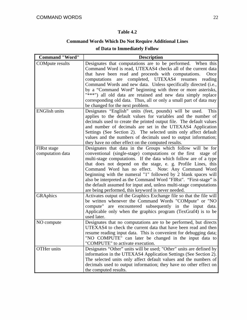
COMMAND WORDS 22
Table 4.2
Command Words Which Do Not Require Additional Lines of Data to Immediately Follow
Command "Word" Description COMpute results Designates that computations are to be performed. When this
Command Word is read, UTEXAS4 checks all of the current data that have been read and proceeds with computations. Once computations are completed, UTEXAS4 resumes reading Command Words and new data. Unless specifically directed (i.e., by a “Command Word” beginning with three or more asterisks, "***") all old data are retained and new data simply replace corresponding old data. Thus, all or only a small part of data may be changed for the next problem.
ENGlish units Designates “English” units (feet, pounds) will be used. This applies to the default values for variables and the number of decimals used to create the printed output file. The default values and number of decimals are set in the UTEXAS4 Application Settings (See Section 2). The selected units only affect default values and the numbers of decimals used to output information; they have no other effect on the computed results.
FIRst stage computation data
Designates that data in the Groups which follow will be for conventional (single-stage) computations or the first stage of multi-stage computations. If the data which follow are of a type that does not depend on the stage, e. g. Profile Lines, this Command Word has no effect. Note: Any Command Word beginning with the numeral "1" followed by 2 blank spaces will also be interpreted as the Command Word "FIRst". “First-stage” is the default assumed for input and, unless multi-stage computations are being performed, this keyword is never needed.
GRAphics Activates output of the Graphics Exchange file so that the file will be written whenever the Command Words "COMpute" or "NO compute" are encountered subsequently in the input data. Applicable only when the graphics program (TexGraf4) is to be used later.
NO compute Designates that no computations are to be performed, but directs UTEXAS4 to check the current data that have been read and then resume reading input data. This is convenient for debugging data; "NO COMPUTE" can later be changed in the input data to "COMPUTE" to activate execution.
OTHer units Designates “Other” units will be used; "Other" units are defined by information in the UTEXAS4 Application Settings (See Section 2). The selected units only affect default values and the numbers of decimals used to output information; they have no other effect on the computed results.

COMMAND WORDS 23
Table 4.2 - continued
Command Words Which Do Not Require Additional Lines of Input
Command "Word" Description SECond stage computation data
Designates that data in the Groups which follow will be for the second and third stages of multi-stage computations. If the data are of a type that does not depend on the stage, e. g. Profile Lines, this Command Word has no effect. Note: Any Command Word beginning with the numeral "2" followed by 2 blank spaces will also be interpreted as the Command Word "SECond". “First-stage” is the default assumed for input and, unless multi-stage computations are being performed, this keyword is not used.
SIUnits /or/ SI
Designates “SI” units (meters, Newtons) will be used. This applies to the default values for variables and the number of decimals used to create the printed output file. The default values and number of decimals are contained in the UTEXAS4 Application Settings (See Section 2). The selected units only affect default values and the numbers of decimals used to output information; they have no other effect on the computed results.
UT3 (UTEXAS3 input format).
Forces UTEXAS4 to use the UTEXAS3 input format for compatibility with UTEXAS3 data files. Default is to use the UTEXAS4 format.
UT4 (UTEXAS4 input format).
Used to reset the input data format to UTEXAS4 format if it has previously been set to UTEXAS3 format (See Command Word “UT3”). This is the default, i. e. the UTEXAS4 input format is normally used.
*** (3 or more asterisks)
Separates one entirely different set of data from another. When this “Command Word” is encountered, all existing data are deleted and completely new data must be read in. If an error is encountered in one data set, UTEXAS4 will read ahead until it encounters a line with 3 or more asterisks or the end of file. If a line with 3 or more asterisks is encountered, UTEXAS4 will resume reading new data even though an error has been encountered in earlier data.

COMMAND WORDS: HEADING, LABEL
24
SECTION 5 - GROUP A DATA FOR HEADING AND LABELS (Optional)
Introduction
The Group A data include two types of alphanumeric heading (title) information. The first type is the problem heading information, which consists of one or more lines of text that are written as headings for the output tables. When heading data are entered as input the heading is used for writing output until a new heading is entered. The heading may be changed at any stage of the input data; the heading can be changed between each group of data (B, C, D etc.) or it can be left the same for all groups of input data.
The second type of Group A data are the "label" data. Labels are used to identify each set of data when the data are subsequently read into TexGraf4 from the Graphics Exchange File created by UTEXAS4. Labels appear as text in a "UTEXAS" menu in TexGraf4 and are used to identify data sets for the purpose of setting parameters that control what and how the data are displayed. Labels have no purpose and are ignored unless TexGraf4 is used. Also, labels do not have to be entered with the UTEXAS4 input data even if TexGraf4 is used; the first line of the heading data described above will be used as a label if no labels are entered.
Heading Data Input
You enter a heading or change the current heading by entering the Command Word "HEA" (or "HEADING"), followed by one or more lines of text containing the heading. A blank heading (no heading) is assumed initially and immediately after "***" is encountered in the Command Words. The form of input of heading data is shown in Table 5.1. Sample heading data are shown in Table 5.2.
Label Data Input
Labels are entered by entering the Command Word "LAB" (or "LABEL"), followed by a single line of text containing the label. In general when labels are entered a label will be entered for each data set in the file, i. e. sometime prior to each issuance of the "COMPUTE"
COMMAND WORDS: HEADING, LABEL 25
or "NO COMPUTE" Command Words. The form of input for label data is shown in Table 5.3. Sample label data are shown in Table 5.4.

COMMAND WORDS: HEADING, LABEL 26
TABLE 5.1
Group A - Heading Data Input Format
Input Line
Data Field
Variable/Description
1 1 Command Word: "HEA" (or "HEADING") 2 1 Line of text for heading; up to 80 alpha-numeric characters per line
including blanks.
Repeat Line 2 for additional lines of text in the heading. There are no limits on the number of lines in the heading, Input a blank line to terminate the heading data.
Resume input with Command Words after the heading has been entered.
TABLE 5.2
Sample Heading Data HEAding data follow – This is the first line of the sample heading This is the second line of the sample heading <blank line required here to terminate heading data>
TABLE 5.3
Group A - Label Data Input Format
Input Line
Data Field
Variable/Description
1 1 Command Word: "LAB" (or "LABEL") 2 1 Line of text for label; up to 80 alpha-numeric characters including
blanks.
Resume input with Command Words after the label has been entered.
TABLE 5.4
Sample Label Data LABel data follow – My First Data Set Label

COMMAND WORD: PROFILE LINES
27
Section 6 - GROUP B DATA FOR PROFILE LINES
Introduction
Group B data consist of the "Profile Lines," which are used to describe the geometry of the soil profile and slope cross-section. Individual Profile Lines are defined by the coordinates of a series of points along each line from left-to-right. The points are assumed to be connected by straight lines to represent a continuous, piecewise linear, line.
Beneath a given Profile Line the soil or other material is considered to be of a given type until another Profile Line is encountered. Each Profile Line has a "Material Number" associated with it; the material number is specified as part of the input data for the Profile Line. The material number indicates which set of material properties, (specified in the Group C data - see Section 7), are to be used for the soil beneath the Profile Line. Several Profile Lines may have the same material number.
Segments or portions of segments of two different Profile Lines cannot coincide. If two segments coincide, it is not possible for UTEXAS4 to logically determine which of the two segments (Profile Lines) is to be associated with the underlying material. An error condition is set when two Profile Line segments coincide.
Relationship Between Profile Lines and Slope Geometry
UTEXAS4 permits you to describe a soil profile with "Profile Lines" and, then, consider several slope geometries "cut" from the soil profile. Thus, the Profile Lines do not necessarily define the slope geometry, although they can. Optional slope geometry data can be input as Group F data and when separate slope geometry data are input they govern the slope geometry; several sets of slope geometry (Group F) data may be input for a given set of Profile Lines.
The option of considering several slopes in a given soil profile is useful for embankment and excavated slope design. In the case of embankments (fills) the Profile Lines should include sufficient soil to encompass any potential embankment cross-section; slope geometry data will define the actual embankment geometry and excess soil above the slope will be ignored. In the case of excavated slopes the Profile Lines should define the original soil profile before excavation. The slope geometry data will define the excavated slope profile.

COMMAND WORD: PROFILE LINES 28
The slope geometry (Group F) data are optional; if they are omitted, UTEXAS4 automatically generates the slope geometry using the uppermost Profile Line(s) to create a surface profile. Once Profile Lines have been input and slope geometry data have been defined, either by Group F data or by generating them from the Profile Line data, the slope geometry remains in effect until specific action is taken to change the slope geometry by entering new Group F data. Even if new Profile Line data are entered the slope geometry data will not be revised. If new slope geometry data are required to accompany new Profile Line data, the new slope geometry must either be input as Group F data or a "Null" set of slope geometry data must be input as described in Section 9. New slope geometry data will be generated if a Null set of data is entered for the slope geometry.
Input Data Format
Once Profile Lines are defined, they ordinarily remain in effect until specifically replaced, one-by-one by new data. For example, suppose that five Profile Lines are initially defined and at a later time new data are input for just one Profile Line. The new data may replace one of the "old" Profile Lines, the other four Profile Lines being unchanged, or the new data may add to the old Profile Lines, creating a total of six Profile Lines. Whether the new data replace or add to the old data will depend on the number, nprofile, of the new Profile Line. If a line having the same number as the new line already exists, it will be replaced by the new data. If no line with the number of the new Profile Line exists, the new line is added to the previous lines. The only times Profile Line data are started entirely anew is when asterisks (***) have been input as a Command Word (See Table 4.2).
You enter Profile Line data by entering the Command Word "PRO" (or "PROFILE LINES"), followed by the Profile Line data. Profile Line data may be entered in two different modes: Standard and Import. In the "Standard" mode the Profile Line data are included as part of the input file, immediately following the Command Word "PRO". In the "Import" mode the Profile Line data are read from a separate input file. Profile line data are entered using the Import mode when the Profile Line data have been created separately by another "preprocessor" program. For example, some finite element seepage programs have the capabilities for generating Profile Line data from a finite element mesh.
The mode for input for Profile Line data is designated in the input data by the contents of the first line of data following the Command Word "PRO". If the first line of data following the Command Word begins with a numerical value (i. e. the number of the Profile Line) the Standard mode of input is assumed. If, instead, the first line of data after the Command Word begins with a non-numeric character, the Import mode of input is assumed. In this case the line of input following the Command Word must contain the name of the file from which the input data are to be read. The file containing the Profile Line data should be located in the same directory as the input file. If the file is not found, you will be prompted to enter a valid file name.
COMMAND WORD: PROFILE LINES 29
The format for input of data in the Standard mode is described in Table 6.1; Table 6.2 describes the form for input in the Import Mode. Sample data are presented in Tables 6.3 and 6.4 for Standard and Import modes, respectively. Table 6.5 presents a sample file of Profile Line data to be read as an "import file".

COMMAND WORD: PROFILE LINES 30
TABLE 6.1
Group B - Profile Line Data Input Format - Standard Mode
Input Line
Data Field
Variable/Description
1 1 Command Word: "PRO" (or "PROFILE")
2 1 Number of the Profile Line (nprofile) to be defined next, i.e., on Line(s) 3 below. Profile Line numbers must be in the range of from 1 to 2,147,483,647. Any sequence of numbering and input of Profile Lines may be used.
2 2 Number of the material (nmaterial) for the material beneath the current Profile Line.
2 3 Alphanumeric character(s) or character string(s) to be printed as a label for the Profile Line. Can be as many characters and/or blanks as will fit on a 128-character line of input (including Fields 1 and 2). Can also be entirely blank.
3 1 X coordinate of point on the Profile Line (xprofile) which is currently being defined.
3 2 Y coordinate of point on the Profile Line (yprofile) which is currently being defined.
(a) Repeat Line(s) 3 for additional points on the Profile Line in a left-to-right sequence. More than one pair of coordinates may be entered on a given line of input data if desired; however, each line must contain complete pairs (2 values) for each point. Enter a blank line to terminate data for the current Profile Line.
(b) Repeat Lines 2 and 3, as sets, for additional Profile Lines. Lines may be input in any order. Line numbers, nprofile, may be missing from a sequence; however, there appears to be little need for omitting numbers from a sequence. Enter two blank lines after the very last line of non-blank Profile Line data to terminate all Group B data and return to input of Command Words.

COMMAND WORD: PROFILE LINES 31
TABLE 6.2
Group B - Profile Line Data Input Format - Import Mode
Input Line
Data Field
Variable/Description
1 1 Command Word: "PRO" (or "PROFILE") 2 1 The character string “FILE” followed by the name of the "import"
file that contains the Profile Line data, e. g. “FILE MyProfileData” (quote marks are for clarity, but should not be included in the actual input data). The file must be in the same directory as the current input file. If the file cannot be located and opened, you will be prompted to enter the name of a valid input file.
Note: The input data for Profile Lines in the import file are in the same format as the input data in the Standard Mode (See Lines 2 and 3 - Table 6.1). The first line of data in the import file begins with the Profile Line number, material number, etc. for the first Profile Line; no Command Word is included in the import file.
TABLE 6.3
Sample Profile Line Data - Standard Mode PROfile line data follow – 1 1 Embankment 0.0 0.0 45.0 20.0 150.0 20.0 <blank line required to terminate 1st profile line> 2 2 Upper Sand Layer -100.0 0.0 150.0 0.0 <blank line required to terminate 2nd profile line> 3 3 Clay Layer -100.0 -10.0 150.0 -12.0 <blank line required to terminate 3rd profile line> 4 2 Lower Sand Layer -100.0 -15.0 150.0 -16.0 <blank line required to terminate 4th profile line> <2nd blank line required to terminate all profile line data>

COMMAND WORD: PROFILE LINES 32
TABLE 6.4
Sample Profile Line Data - Import Mode PROfile line data follow – FILE MyProfileData.dat
TABLE 6.5
Sample "Import" File (= MyProfileData.dat) of Profile Line Data 1 1 Embankment 0.0 0.0 45.0 20.0 150.0 20.0 <blank line required to terminate 1st profile line> 2 2 Upper Sand Layer -100.0 0.0 150.0 0.0 <blank line required to terminate 2nd profile line> 3 3 Clay Layer -100.0 -10.0 150.0 -12.0 <blank line required to terminate 3rd profile line> 4 2 Lower Sand Layer -100.0 -15.0 150.0 -16.0 <blank line required to terminate 4th profile line> <2nd blank line required to terminate all profile line data>

COMMAND WORD: MATERIAL PROPERTIES
33
Section 7 - GROUP C DATA FOR MATERIAL PROPERTIES
Introduction
Group C data consist of material properties, which include unit weights, shear strengths, and how pore water pressures, if any, are defined for each material in the soil profile. Each Profile Line has a set of material properties assigned to it; several Profile Lines may share the same set of material properties. The material property data and the form of the input data are described in this section.
Effective Stress Versus Total Stress Analyses
Shear strengths can be defined using either total or effective stresses. For total stresses shear strengths are expressed by the equation,
s = c + σ tan(φ) 7.1
where σ is the total normal stress on the shear plane, and c and φ are shear strength parameters expressed in terms of total stresses. For the case of effective stresses the shear strengths are expressed by
s = c + (σ - u) tan( ) 7.2 φ
where u is the pore water pressure, (σ - u) is the effective normal stress, and c and φ are shear strength parameters expressed in terms of effective stresses. In the input data for UTEXAS4 values for "cohesion" and "friction angle" must be the appropriate total stress (c, φ) or effective stress ( c , φ
) values. The only other distinction that is made between total and effective stresses in the input data is that for effective stresses appropriate pore water pressures (including zero as a special case) must be specified; for total stresses pore water pressures must be specified as zero2.
The distinction between total and effective stresses is made on a material-by-material basis. The shear strengths of some materials may be expressed using total stresses, while the shear strengths for other materials may be expressed using effective stresses.
2 One exception to the case of zero pore water pressure exists for total stress analyses: When shear strengths are defined by a c/p ratio (Shear Strength Option 4) non-zero pore water pressures may be specified even though the shear strengths used in the stability calculations are expressed as total stress values. The pore water pressures that are specified in the input data are used to compute the effective consolidation stresses; they are not actually used in computing the stability. Eq. 7.1 and total stresses are used to express the shear strength in the stability calculations.

COMMAND WORD: MATERIAL PROPERTIES 34
Properties for Multi-Stage Computations
When UTEXAS4 is used for two-stage or three-stage stability computations, two complete sets of properties (shear strengths, unit weights and pore water pressures) must be entered for the different stages of the analysis. The first set of properties is used for the first stage computations; the second set of properties is used for the second and third stage computations. Material properties for the first stage computations are the same as those for conventional, single-stage computations. Depending on the type of soil, the properties and data for the second stage of computations may be the same or almost the same as those for the first stage. For example, in freely draining materials strengths are specified using effective stresses for both stages. The strength parameters and method for describing pore water pressures (e. g. a piezometric line) may be the same for both stages; only the unit weights may change. For other materials properties for the second stage will be different from those for the first stage. Usually, for the second stage "two-stage" strengths will be defined. Two special “two-stage” shear strength options (Options 8 and 9) exist for defining shear strengths for the second stage. Option 8 employs linear shear strength envelopes; option 9 employs nonlinear envelopes. The distinction between which set of material properties is being input at any time is made using the Command Words FIRst and SECond as described in Section 4.
Unit Weights
The unit weight for each material should be the total unit weight (total weight divided by total volume). In two cases the submerged (buoyant) unit weight of soil may be used; however, even for these two cases it is not necessary to use submerged unit weights. The use of submerged unit weights is not recommended. The two cases where submerged unit weights may be used (but are not recommended) are described below:
1. Submerged unit weights may be used for total stress analyses where φ is equal to zero and some portion of the slope is submerged. Submerged unit weights may be used for the portion of soil which is submerged beneath water provided that the water level is horizontal3. If the submerged unit weight is used, any distributed loads due to the overlying water must not be specified in the input data (See Section 11 for description of Distributed Loads); the effects of the surface loads are already accounted for when the submerged unit weight is used. If there is flow of water (sloping water surface) or φ is not equal to zero, submerged unit weights should not be used for total stress analyses.
3 While, technically, submerged unit weights can be used when the water level in the slope is inclined, submerged unit weights cannot be used for all the soil beneath the inclined water surface. This, leads to further complications in applying submerged unit weights and emphasizes the advantage of not using of submerged unit weights.

COMMAND WORD: MATERIAL PROPERTIES 35
2. Submerged unit weights may also be used for effective stress analyses where the slope is partially or fully submerged. Submerged unit weights may be used for the submerged portion of soil provided that there is no flow of water and no hydraulic gradient4. If the submerged unit weight is used, pore water pressures and any distributed loads due to the water must not be specified in the input data; the effects of pore water pressures and surface pressures are already accounted for when the submerged unit weights are used.
If submerged unit weights are used for one material, they must be used for all materials where submerged unit weights are applicable, i.e., they must be used for all portions of materials which are submerged.
Shear Strength Options
Ten options are available for defining shear strengths for each material. Two options (8 and 9) are used to define "two-stage" strengths for multi-stage (two-stage and three-stage) slope stability computations. The other options (1 through 7, and 10) may be used for either conventional analyses, or for the first or second stage of multi-stage analyses if appropriate. The ten options are described below:
Option 1 (Conventional c, φ Strength)
The shear strength is isotropic (shear strength is independent of the orientation of the failure plane) and is defined by cohesion (c) and friction angle (φ) corresponding to the intercept and slope of the Mohr-Coulomb failure envelope. For total stress analyses the cohesion and friction angle are the values of c and φ determined using total stresses to plot the failure envelope. In this case the pore water pressures must be specified to be zero. For effective stress analyses the values of c and φ ( c and φ
) should be values determined using effective stresses to plot the failure envelope. In the case of effective stresses appropriate pore water pressures will need to be specified; pore pressures may or may not be zero.
Option 2 (Linear Increase Below Profile Line)
The shear strength varies linearly with depth below the Profile Line(s) which have this shear strength characterization. The value of the shear strength at the Profile Line and the rate of increase in shear strength with depth below the Profile Line are entered as input data. A negative value for the rate of "increase" is interpreted as a decrease in shear strength with depth below the Profile Line and an increase in shear strength above the Profile Line.
The friction angle is assumed to be zero for Option 2 and the appropriate shear strength, depending on depth, is assigned as a cohesion value for the stability computations.
4 A hydraulic gradient may exist with no or negligible flow, e. g. when there are different water levels each side of an impervious barrier. Submerged unit weights should not be used in these cases even though there is no flow.

COMMAND WORD: MATERIAL PROPERTIES 36
Accordingly, Option 2 will generally only apply to cases where the soil is saturated and the loading is undrained; computations are performed using total stresses.
Option 3 (Linear Increase Below Horizontal Reference)
The shear strength varies linearly with depth below a selected reference datum. The elevation (y) of the reference datum, the value of the shear strength at the elevation of the reference datum, and the rate of increase in shear strength with depth below the datum are input as data by the user. Option 3 is similar to Option 2. The only difference between the two options is that for Option 3 the shear strength varies with depth below a horizontal datum, while for Option 2 the datum is the Profile Line, which may or may not be horizontal.
Shear strength is assumed to decrease with depth above the reference datum at the same rate that it increases with depth below the datum. A negative value for the rate of "increase" is interpreted as a decrease in shear strength with depth below the reference datum and an increase in shear strength above the datum.
The friction angle is assumed to be zero for Option 3. Like Option 2, Option 3 will generally only apply to cases where the soil is saturated and the loading is undrained; computations are performed using total stresses.
Option 4 (Constant c/p Ratio)
The shear strength is defined by a constant c ratio representing the ratio of shear strength to effective vertical consolidation pressure. The shear strength is computed according to the following relationship:
/ p
s c u cpo v= + −σb g 7.3
where, represents the shear strength for zero effective consolidation pressure, (σv - u) represents the effective vertical consolidation pressure, and
co
c / p
o
represents the rate of increase in shear strength with increase in vertical effective stress. Values of the intercept shear strength ( c ) and c / ratio are entered as input data when this option is chosen. The effective vertical consolidation pressure is computed by subtracting the pore water pressure (u) from the total vertical consolidation stress (
p
σv ).
The shear strength is computed from Eq. 7.3 at the center of the base of slices. The vertical stress (σv) is computed by dividing the total weight of the slice by the width of the slice; distributed loads acting on the surface of the slope and line loads are not included in the computation of the vertical stress. The pore water pressure is computed from information entered for pore water pressures for the material. In this case pore water pressure information entered with the material properties is used to compute effective consolidation pressures, which in turn are used to compute shear strengths from Eq. 7.3. Once the shear strengths are computed they are assigned to the bases of the slices as values of cohesion and

COMMAND WORD: MATERIAL PROPERTIES 37
the friction angle is set to zero. The pore water pressures do not appear directly in the stability equations and will not directly affect the subsequent computations for the factor of safety, they only affect the value of effective stress that is used to calculate the shear strength beforehand.
When this strength option is chosen minimum and maximum shear strengths are entered in addition to the values of and co c / p . The value computed from Eq. 7.3 is compared with the minimum and maximum strengths entered and if the value lies outside the minimum or maximum value it is set equal to the appropriate minimum or maximum. Thus, the variation in shear strength with effective stress might follow a pattern like the one shown by the heavy, solid line in Fig. 7.1.
Option 5 (Anisotropic Strengths)
The shear strength parameters c and φ (or c and φ ), vary with the orientation of the failure plane. Values of c and φ are input for selected failure plane orientations and linear interpolation is used to obtain values at orientations between the specified values. UTEXAS4 will later assign appropriate values of c and φ to each slice based on the orientation of the base of the slice; the base of the slice is considered to represent the failure plane. The inclination of the failure plane is assumed to be the inclination of the base of the slice. (See Section 14 regarding subdivision of the soil mass into slices).
Failure plane orientations are specified in the input data by angles measured in degrees from the horizontal plane. Positive angles correspond to positive slopes (dy/dx) of the shear surface and negative angles correspond to negative slopes (Fig. 7.2). Failure plane orientations may range from negative to positive and should encompass the maximum anticipated range of failure plane (shear surface) inclinations. UTEXAS4 will not extrapolate from the input data for angles outside the range covered by the input data. When the inclination of the failure plane lies outside the range specified by the data an error message is issued.
The shear strength, especially the undrained shear strength, should depend on not only the direction of the failure plane, but also on the direction of shear: Shear in one direction along a plane may produce a different shear strength than shear in the opposite direction due to differences in the directions of the principal stresses. Accordingly, it may be necessary to use separate sets of anisotropic shear strength input data to analyze both the left and the right faces of a slope.
Option 6 (Nonlinear, Curved Failure Envelope)
The shear strength ("Mohr-Coulomb" type) envelope is non-linear, i.e., it is not a single straight line. Values of shear strength (τ) are input for various values of total or effective normal stress (σ or σ ) to define points on a nonlinear shear strength envelope as shown in Figure 7.3. The points are assumed to be connected by straight lines to form a

COMMAND WORD: MATERIAL PROPERTIES 38
piecewise linear envelope. UTEXAS4 assigns a shear strength to the base of each slice based on the total or effective normal stress on the base of the slice (See Section 14 regarding slices). An iterative procedure is used to assign the shear strengths because the computed normal stresses depend on the shear strength. The computed normal stresses also depend on the factor of safety. Accordingly, shear strengths defined by a nonlinear shear strength envelope are assigned at the time the factor of safety is computed. Because the solution for the factor of safety involves using a trial and error procedure, two levels of iteration are required when a nonlinear shear strength envelope is used: One level of iteration ("inner loop") is required to solve the equilibrium equations for the factor of safety; the other level ("outer loop") is for the nonlinear shear strength envelope.
UTEXAS4 will not extrapolate from the input data for values of the normal stress outside the range covered by the input data. When the normal stress falls outside the range of the data an error message is issued. To prevent this from happening points may need to be defined on the shear strength envelope for negative as well as positive normal stresses, especially if the shear strength envelope has a "cohesion" intercept. Frequently the shear strength values (τ) for negative normal stresses will be defined to be zero, i. e. there will be no tensile strength.
Option 7 (Interpolation of Strength)
For Option 7 the shear strengths are determined by interpolation from data specified at discrete "interpolation points". The interpolation scheme is identical to the scheme used to interpolate pore water pressures and is described in further detail in Section 9 on the Group E Data for interpolation points. (Note: With Option 7 the Group C Material Property data only designate that the shear strengths are determined by interpolation; the actual data points used for the interpolation are input as Group E Data).
The shear strength interpolation option (Option 7) is intended for use where a detailed assessment of shear strength has been made using procedures like the SHANSEP procedure where shear strengths are related to consolidation stress history. It is NOT intended to serve as a means for filling in shear strength values in the interval between widely spaced borings or similar situations where data are sparse and must be estimated based on judgment. The interpolation scheme is not intended to supplant judgment, but rather to provide a means of interpolating strength to points along a shear surface from nearby points where you have already defined the shear strength. Shear strenngths are interpolated to the center of the base of each slice.
Two values, representing the maximum and minimum allowable strengths, are entered with the Group C Material Property Data (in addition to the data points entered as Group E Data). The minimum and maximum strengths are imposed as constraints on whatever strength values are calculated by interpolation. When the strengths are actually computed by interpolation from the Group E Data points, the values are compared to the minimum and maximum values entered with the Material Property Data. If the interpolated

COMMAND WORD: MATERIAL PROPERTIES 39
values of shear strength lie outside the designated minimum or maximum, the values are set equal to the appropriate limit. Once shear strengths have been computed and adjusted for maximum and minimum limits, they are assigned to slices as values of cohesion and the friction angle (φ) is set equal to zero.
Option 8 (Two-Stage Strength - Linear Envelopes)
A "two-stage strength" is defined by two envelopes expressing relationships between the shear stress on the failure place at failure ( τff ) and the effective normal stress on the failure plane at consolidation ( σfc ). Each envelope corresponds to a given effective principal stress ratio, Kc = σ 1c/ σ 3c for consolidation, where σ 1c and σ 3c represent major and minor principal effective stresses, respectively. The first envelope is for an effective principal stress ratio of unity (Kc = 1). This envelope is usually derived from consolidated-undrained triaxial compression tests on specimens which have been consolidated isotropically. The second envelope corresponds to the maximum possible effective principal stress ratio for consolidation (Kc = Kfailure) and is identical to the conventional effective stress shear strength envelope derived from either consolidated drained (CD, S) or consolidated-undrained ( CU , R ) triaxial tests with pore water pressure measurements. Each envelope is defined by its intercept value, d, and slope angle, Ψ (Fig. 7.4). The two-stage shear strength envelopes and their use are described in further detail in Appendix A. Although the failure envelope corresponding to (Kc = Kf) for the two-stage strengths is usually identical to the effective stress envelope used for the first stage computations, the envelope must be specified again in the input data for the second stage computations.
Option 9 (Two-Stage Strength - Nonlinear Envelopes)
Two nonlinear (piecewise linear) shear strength envelopes are defined for Option 10. This option is identical to Option 9 except the shear strength envelopes are nonlinear. One envelope is the same as the effective stress envelope and corresponds to an anisotropic consolidation stress ratio, Kc = K f ; the other envelope is the envelope of τff versus σ
_fc
corresponding to isotropic consolidation ( Kc = 1). Each of the two nonlinear strength envelopes is defined in terms of points on the envelope, connected by straight lines. The envelopes are defined like the nonlinear envelope for strength Option 6. An effective normal stress and corresponding values of shear stress for the two envelopes are entered as data. Points on each envelope share common values of effective normal stress. Accordingly, whenever there is a break in either of the two envelopes a point must be defined on both envelopes (Fig. 7.5).
Option 10 ("Very High" Strengths)
This option is used to designate a material as having a shear strength that is sufficiently high to prevent any potential shear surface from passing through it. For example, this may be used to describe the shear strength for a material in the cross-section representing concrete, e. g. a retaining wall. If any shear surface intersects a material with this (very high)

COMMAND WORD: MATERIAL PROPERTIES 40
strength option, the shear surface is automatically rejected and no attempt is made to compute a factor of safety for that particular shear strength. In this special case (and only for Option 10) no separate pore water pressure data are entered with the material properties.
Pore Water Pressure Options
Six options are available for defining pore water pressures for each material as follows:
Option 1 (No Pore Water Pressure)
The pore water pressures are assumed to be zero - total stresses are being used, or the actual pore water pressures are equal to zero.
Option 2 (Constant Pore Water Pressure)
The pore water pressure is constant throughout the given material; the constant value of pore water pressure is then input. This option is seldom used.
rOption 3 (Constant Pore Water Pressure Coefficient, u )
The pore water pressures are expressed by a constant, value of the pore water pressure coefficient, ru (Bishop and Morgenstern, 1960). The pore water pressure coefficient is defined as
r uhu =
γ
rr
6.3
where u is the pore water pressure at any point and γh is the corresponding total vertical stress (overburden pressure). If this option is chosen, the value of u is entered as input. In computing pore water pressures using a value of u UTEXAS4 calculates "γh" due to the weight of overlying soil, but excludes any added vertical stress due to Distributed Loads or Line Loads (Sections 11 and 12).
Option 4 (Piezometric Line)
For Option 4 the pore water pressure is defined by a piezometric line; piezometric line data must be input separately as Group D data (Section 8). Each piezometric line is numbered. If this option is chosen for pore water pressures the identification number for the piezometric line to be used for each material is entered with the material property data.
In computing pore water pressures from the piezometric line UTEXAS4 calculates the vertical distance between the point of interest and the piezometric line and multiplies this distance by the unit weight of water to arrive at the pore water pressure. Pore water pressures

COMMAND WORD: MATERIAL PROPERTIES 41
are assumed to be positive below the piezometric line and negative above the piezometric line (See Section 8 for more details on piezometric lines).
Option 5 (Pressure Interpolated)
Pore water pressures are computed by interpolating pore water pressures from an irregular "grid" of pore water pressure values. The grid of pore water pressure values is specified separately as Group E data (See Section 9).
Option 6 (Pressure Coefficients, ru , Interpolated)
Pore water pressures are computed by interpolating in a manner similar to that for Option 5, except that values of the pore water pressure coefficient, u , rather than actual values of pressure, are input and used for interpolation. The values of u are used and defined in the same manner as described for Option 3. Further description of the interpolation is presented in Section 9. Option 6 is seldom used.
rr
Negative Pore Water Pressures
Normally, UTEXAS4 sets any negative value of pore water pressure to zero before proceeding with further calculations; however, you can optionally override this feature if you want (See Line No. 6, Field No. 3 in Table 6.1).
Input Data Format
The form and guide for Group C data input are presented in Table 7.1. The Group C data must immediately follow the Command Word "MAT" (or "MATERIAL PROPERTIES").
Once data have been input for materials, the data remain in effect until specifically replaced, material by material, with new data. If new data are input for only one material, after data for several materials have been input previously, then the new data will either replace the data for one material or add to the existing data. If the material number ( n - See Line No. 2, Field No. 1 of Table 7.1) for the new material is identical to one previously defined, the new data will
material
replace the previous data for this material only. If the number for the new material has not been previously defined, the new data are added to the old data which were previously defined. The only time material property data are started entirely anew is when asterisks (***) have been input as a Command Word (See Table 4.2).

COMMAND WORD: MATERIAL PROPERTIES 42
Sample data for shear strength options applicable to both conventional (single-stage) and multi-stage computations are presented in Table 7.25. Sample data for two-stage strengths are presented in Table 7.3 (Note: Both single-stage and two-stage strength formats may be used for the second-stage input data.)
5 Theses sample data are intended for illustration only and contain an unusual mix of shear strength data expressed in terms of total and effective stresses. Although the data can be read and used by UTEXAS4, they should not be considered representative of material properties for a given problem.

COMMAND WORD: MATERIAL PROPERTIES 43
TABLE 7.1
Group C - Material Property Data Input Format
Input Line
Data Field
Variable/Description
1 1 Command Word: "MAT" (or "MATERIAL PROPERTIES")
2 1 Number (nmaterial) used to identify the material for which data will follow on Line(s) 3 through 7. This number corresponds with the material numbers input for Profile Lines in the Group B data.
2 2 Any alphanumeric character(s) or character string(s) to be printed as a label with data for this material. Can be as many characters and/or blanks as will fit on a 128-character line of input (including Field 1). Can also be blank.
3 1 Unit weight for the current material. 4 1, 2 A character or character string beginning with the appropriate character,
to designate how shear strengths are to be characterized for the current material. The acceptable character or character string and its interpretation are shown below. The key character(s) which must be input are capitalized and underlined. (Note: Only the first non-blank character of each string is recognized and used.)
Character String Interpretation Conventional /or/
Isotropic (C or I) Shear strengths are expressed by conventional Mohr-Coulomb parameters, c and φ. Follow this line of data with line 5A below. NOTE: Only one character or character string should be entered to avoid confusion with ”C P” sequence below.
Linear (L) Shear strengths increase linearly with depth below the Profile Line, starting at a prescribed value along the Profile Line. Follow this line of data with Line 5B below.
Reference (R) Shear strengths increase linearly with depth below a horizontal datum specified by its reference elevation. Follow this line of data with Line 5C below.
(continued on next page)

COMMAND WORD: MATERIAL PROPERTIES 44
TABLE 7.1 - continued
Group C - Material Property Data Input Format
Input Line
Data Field
Variable/Description
4 1,2 Cover P ratio (C P)
The shear strength is characterized in terms of a constant c/p ratio. Follow this line of data with Line 5D below. NOTE: The second leading character (P) distinguishes this option from the "conventional" shear strength option. The second character must be a "P", e. g. "C over P" will result in the incorrect interpretation as "C o".
Anisotropic shear (A) Shear strengths vary with the orientation of the failure plane. Follow this line of data with Lines 5E below.
Nonlinear Mohr- Coulomb envelope (N)
The shear strength envelope is nonlinear. Follow this line of data with Lines 5F below.
Interpolate Strengths (I S)
The shear strengths are to be determined by interpolation of values of shear strength specified at prescribed locations. Follow this line of data with Lines 5G below. NOTE: The second leading character (S) distinguishes this option from the "isotropic/conventional" shear strength option.
Very Strong material (V S)
The soil is assumed to be infinitely strong. Any shear surface passing through the material is rejected for computing the factor of safety. Line Nos. 5, 6 and 7 are not required - omit them.
2-stage Linear strength envelopes (2 L)
The shear strength is a "two-stage" strength and the shear strength envelopes are straight lines (linear). Follow this line of data with Lines 5H below. (Applicable only when strengths are being entered for the second stage - otherwise an error condition will result.)
2-stage Nonlinear strength envelopes (2 N)
The shear strength is a "two-stage" strength and the envelope(s) are not linear. Follow this line of data with Lines 5I below. (Applicable only when strengths are being entered for the second stage - otherwise an error condition will result.)
(continued on next page)
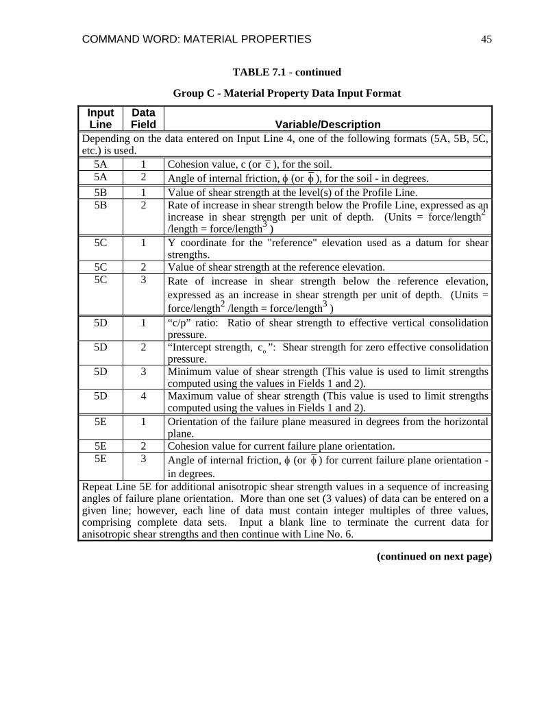
COMMAND WORD: MATERIAL PROPERTIES 45
TABLE 7.1 - continued
Group C - Material Property Data Input Format
Input Line
Data Field
Variable/Description
Depending on the data entered on Input Line 4, one of the following formats (5A, 5B, 5C, etc.) is used.
5A 1 Cohesion value, c (or c ), for the soil. 5A 2 Angle of internal friction, φ (or φ ), for the soil - in degrees. 5B 1 Value of shear strength at the level(s) of the Profile Line. 5B 2 Rate of increase in shear strength below the Profile Line, expressed as an
increase in shear strength per unit of depth. (Units = force/length2 /length = force/length3 )
5C 1 Y coordinate for the "reference" elevation used as a datum for shear strengths.
5C 2 Value of shear strength at the reference elevation. 5C 3 Rate of increase in shear strength below the reference elevation,
expressed as an increase in shear strength per unit of depth. (Units = force/length2 /length = force/length3 )
5D 1 “c/p” ratio: Ratio of shear strength to effective vertical consolidation pressure.
5D 2 “Intercept strength, c ”: Shear strength for zero effective consolidation pressure.
o
5D 3 Minimum value of shear strength (This value is used to limit strengths computed using the values in Fields 1 and 2).
5D 4 Maximum value of shear strength (This value is used to limit strengths computed using the values in Fields 1 and 2).
5E 1 Orientation of the failure plane measured in degrees from the horizontal plane.
5E 2 Cohesion value for current failure plane orientation. 5E 3 Angle of internal friction, φ (or φ ) for current failure plane orientation -
in degrees. Repeat Line 5E for additional anisotropic shear strength values in a sequence of increasing angles of failure plane orientation. More than one set (3 values) of data can be entered on a given line; however, each line of data must contain integer multiples of three values, comprising complete data sets. Input a blank line to terminate the current data for anisotropic shear strengths and then continue with Line No. 6.
(continued on next page)

COMMAND WORD: MATERIAL PROPERTIES 46
TABLE 7.1 - continued
Group C - Material Property Data Input Format
Input Line
Data Field
Variable/Description
5F 1 Normal stress, σ (or σ ), for point on the nonlinear failure envelope 5F 2 Shear stress, τ, for point on the nonlinear envelope.
Repeat Line 5F for additional values to define a nonlinear failure envelope. Values must be input in a sequence of increasing values of normal stress. More than one pair of values (σ and τ) can be entered on a single line of input data if desired; however, pairs of values (even multiples of two) must always be entered on each line. Input a blank line at the end of the data for the nonlinear failure envelope.
5G 1 Minimum value allowed for interpolated strength. If interpolated values are less than this value, they will be set equal to this value.
5G 2 Maximum value allowed for interpolated strength. If interpolated values are greater than this value, they will be set equal to this value.
5H 1 Intercept, d (Kc = 1) for the envelope of τff vs. σfc from isotropically consolidated-undrained triaxial compression tests.
5H 2 Slope, Ψ (Kc = 1) for the envelope of τff vs. σfc from isotropically consolidated-undrained triaxial compression tests.
5H 3 Effective stress cohesion value, c = d (Kc = Kfailure), envelope from consolidated-drained (CD) shear tests or consolidated-undrained shear tests with pore pressure measurement ( CU ).
5H 4 Effective stress angle of internal friction, φ = Ψ (Kc = Kfailure), of envelope from consolidated-drained (CD) shear tests or consolidated-undrained shear tests with pore pressure measurement ( CU ).
5I 1 Effective normal stress on the failure plane at consolidation ( σfc ) for nonlinear two-stage envelope. The shear stresses in the next two fields should correspond to this normal stress.
5I 2 Shear stress on the failure plane at failure ( τff ) for the envelope derived from isotropically consolidated-undrained (CU) triaxial compression tests.
5I 3 Shear stress on the failure plane at failure ( τff ) for the conventional effective stress failure envelope; derived either from consolidated drained (CD) tests or consolidated-undrained shear tests with pore water pressure measurements( CU ).
Repeat Line 5I for additional values to define the complete nonlinear envelopes for the two-stage strengths. Values must be entered in a sequence of increasing values of normal stress. More than one set of values (points) may be entered on a single line of input data if desired; however, each line must contain integer multiples of three values, comprising complete data points. Input a blank line at the end of the nonlinear failure envelope data and proceed with Line No. 6 for the current material.
(continued on next page)

COMMAND WORD: MATERIAL PROPERTIES 47
TABLE 7.1 - continued
Group C - Material Property Data Input Format
Input Line
Data Field
Variable/Description
6 1 and 2 Two characters separated by blanks, or two character strings separated by blanks, to designate how pore water pressures are to be defined for this material. The acceptable characters or character strings and their interpretation are shown below. The key characters which must be input are capitalized and underlined. (Note: Only the first character of any character string is recognized and used.)
Character String Interpretation No pore pressure (N) Pore pressures are zero. (Only one character, N,
is actually required in this case.) No Line 7 is required; see notes following Line No. 7.
Constant Pressure (C P)
Pore pressures are constant. Follow this line of data with Line No. 7 giving the value of the pore water pressure.
Constant Ru (C R)
Pore water pressures are defined by a constant value of the pore water pressure coefficient, ru. Follow this line of data with Line No. 7 giving the value of the pore water pressure coefficient, ru.
Piezometric Line (P L)
A piezometric line is used to define pore water pressures in this material. Follow this line of data with Line No. 7 giving the number of the piezometric line which is to be used. Note: Group D data must eventually be input.
Interpolate Pore Pressures (I P)
Pore water pressures are determined by interpolation of values of pore water pressure. Note: Group E data must eventually be input, but no Line No. 7 is required below. See notes following Line No. 7.
Interpolate Ru values (I R)
Pore water pressures are determined by interpolation of values of the pore water pressure coefficient, ru . Note: Group E data must eventually be input, but no Line No. 7 is required below.
3 Optional designation to allow negative pore water pressures. If negative pore water pressures are allowed, enter the character “N” or a character string beginning with the character “N” to designate that negative pore water pressures are allowed.
(continued on next page)

COMMAND WORD: MATERIAL PROPERTIES 48
TABLE 7.1 - continued
Group C - Material Property Data Input Format
Input Line
Data Field
Variable/Description
7 1 Value of either (a) the pore water pressure, or (b) u or (c) the number of the piezometric line depending on data on Line No. 6. Line 7 is not required where there are either no pore water pressures or pore water pressures are defined by interpolation.
r
Repeat Lines 2 through 7, as sets, for data for additional material properties (material numbers). Material properties for different materials may be input in any order. (Material numbers may actually be missing from a sequence; however, there appears to be little need for omitting numbers from a sequence.) Input a blank line after the data for the last material have been input to designate the end of all Group C data.

COMMAND WORD: MATERIAL PROPERTIES 49
Table 7.2
Sample Material Property Data for Options Applicable to All Stages MATerial property data follow - 1 Slightly over-consolidated clay 118.0 = unit weight Conventional shear strengths 250.0 22.0 Constant R-sub-u 0.15 2 Saturated clay 109.0 = unit weight Linear increase in strength below Prof. Line 200.0 20.0 No pore pressures 3 Saturated clay 114 = unit weight Reference elev. Defined strength increase 75.0 350.0 15.0 Constant pore pressure 0.0 4 Slightly Overconsolidated, Saturated Clay 106 = unit weight C_over P ratio defines strength 0.25 100.0 250.0 2500.0 Piezometric Line 1 5 Heavily Overconsolidated Shale 128 = unit weight Anisotropic shear strengths -90.0 3500.0 0.0 -60.0 3300.0 0.0 -30.0 3000.0 0.0 -5.0 2500.0 0.0 -4.5 1000.0 0.0 4.5 1000.0 0.0 5.0 1500.0 0.0 30.0 1800.0 0.0 60.0 1900.0 0.0 90.0 1950.0 0.0 <blank line terminates anisotropic shear strength values> No pore pressures
(sample data continued on next page)

COMMAND WORD: MATERIAL PROPERTIES 50
Table 7.2 - continued
Sample Material Property Data for Option2 Applicable to All Stages 6 Compacted Clay 122 = unit weight Nonlinear failure envelope -1000.0 0.0 0.0 0.0 300.0 300.0 1000.0 500.0 2000.0 1000.0 10000.0 2500.0 <blank line terminates points on nonlinear failure envelope> Interpolate R-sub-u Values 7 Soft, Saturated Clay 100 = unit weight Interpolate Strengths 250.0 3000.0 No pore pressures 8 Concrete 145 = unit weight Very Strong <blank line terminates all material property data>

COMMAND WORD: MATERIAL PROPERTIES 51
Table 7.3
Sample Material Property Data for Materials with "Two-Stage" Strengths MATerial property data follow - 1 Compacted Sandy Clay 118.0 = unit weight 2_Stage Linear envelope 500.0 10.0 0.0 30.0 Piezometric Line 1 2 Compacted Dense, Sandy Gravel 136 = unit weight 2_Stage Nonlinear envelope 0.0 0.0 0.0 1600.0 600.0 750.0 4400.0 1600.0 3400.0 <blank line terminates points on nonlinear failure envelope> Interpolate Pore pressures <blank line terminates all material property data>

COMMAND WORD: MATERIAL PROPERTIES 52
Undrained Shear Strength, Su
Vertical
Effective
Stress, p
co cminimum cmaximum
1
c/p
Figure 7.1 - General Variation in Undrained Shear Strength When Shear Strengths Are Defined by a Constant c/ p ratio.

COMMAND WORD: MATERIAL PROPERTIES 53
Cohesion, c
FrictionAngle, φ
Failure Plane Angle, α
Failure Plane Angle, α
-90° +90°-60° +60°-30° +30°0°
-90° +90°-60° +60°-30° +30°0°
α (+)
α (-) α (+)
α (-)
Figure 7.2 - Anisotropic Shear Strength Representation and Sign Convention for Failure Plane Orientation.

COMMAND WORD: MATERIAL PROPERTIES 54
She
ar S
tress
, τ
Normal Stress, σ
Figure 7.3 - Nonlinear (Curved) Mohr-Coulomb Failure Envelope.

COMMAND WORD: MATERIAL PROPERTIES 55
She
ar S
tress
, τ
Normal Stress, σ
Kc=1ddKc=Kf
ψKc=Kf
Kc=1ψ
Figure 7.4 - Linear Failure Envelopes Used to Define "Two-Stage" Shear Strengths.

COMMAND WORD: MATERIAL PROPERTIES 56
She
ar S
tress
on
the
Failu
re P
lane
at F
ailu
re,
τ ff
Effective Stress on the Failure Plane at Consolidation, σfc
Figure 7.5 - Nonlinear Failure Envelopes Used to Define "Two_Stage" Shear Strengths

COMMAND WORD: PIEZOMETRIC LINES
57
Section 8 - GROUP D DATA FOR THE PIEZOMETRIC LINE (Optional)
Introduction
Group D data are for "Piezometric Lines", which are used to define pore water pressures in the soil. Pore water pressures are computed from a piezometric line by multiplying the vertical distance between the piezometric line and the point of interest by a unit weight of fluid (normally the unit weight of water). Piezometric line data are generally only required when pore water pressures for one or more materials are defined by a piezometric line (See Material Property Data - Section 7).
Relationship between Piezometric Lines and Surface Water Loads
Piezometric lines ordinarily have no effect on external loads and are not used to compute water loads on the slope or ground surface. In general external water loads must be designated separately by Distributed Load data (See Section 11). In special cases the Distributed Load data can stipulate that a piezometric line is to be used to compute external water loads, but this must be done with the Distributed Load data described in Section 11. In this special case piezometric line data may be required even when piezometric lines are not being used to define pore water pressures in the soil.
Description of Data
Pore water pressures computed from the piezometric line are negative above the piezometric line and positive below the piezometric line. UTEXAS4 normally sets negative values of pore water pressure to zero for the slope stability computations. If negative values are to be used for the slope stability computations, rather than set equal to zero, you must designate this with the material property data for each material where negative pore water pressures are to be used (See Section 7 and Table 7.1, Input Line 6, Data Field 3).
Any number of piezometric lines can be defined. In the input data for each piezometric line the lines are assigned a unique identification number expressed as a positive integer in the range of from 1 to 2,147,483,647. The identification number is used to associate each piezometric line with the material property data (See Table 7.1 - Line No. 7). Several materials may share and use the same piezometric line. The sequence and pattern for assigning numbers to piezometric lines can be chosen arbitrarily.

COMMAND WORD: PIEZOMETRIC LINES 58
Each piezometric line is defined by the coordinates of a series of points from left to right along the line. The points are assumed to be connected by straight lines to form a continuous, piece-wise linear piezometric surface.
Vertical segments of the piezometric lines are acceptable; however, vertical segments are never actually used: Slices are created such that a slice boundary is placed wherever a point is defined on a piezometric line. Pore water pressures are then calculated at the center of the base of each slice, assuring that pore water pressures are never calculated at a point where the piezometric line is vertical. Vertical segments are just allowed to simplify input of a continuous piezometric surface where there is an abrupt change in water pressures.
The unit weight of fluid used to compute pore water pressures from the piezometric line may be input with the piezometric line data or, if no value is input, the default value for the unit weight of fluid is used. The default value for the unit weight of fluid is contained in the UTEXAS4 Application Settings (See Section 2). If the unit weight of fluid is entered with the input data, different values may be entered for each piezometric line. If data are omitted for any piezometric line, default values are used for the unit weight of fluid for the piezometric lines where unit weights are omitted.
Multi-Stage Computations
When multi-stage (two--stage or three-stage) computations are performed, separate sets of piezometric line data are specified for the first and the subsequent (second & third) stages. Piezometric lines specified for the first stage are not used for the second and third stages and vice-versa.
When multi-stage computations are performed the piezometric line data entered for the second stage are used differently depending on the type of material (shear strength option). For materials with strength Options 1 through 7 the piezometric line data for the second stage are used to compute pore water pressures for the second stage computations and the third stage computations as well (if third stage computations are performed). Normally any materials with strength Options 1 through 7 that have pore water pressures defined by piezometric lines will be free-draining materials. For materials which have "two-stage" strengths (Strength Options 8 and 9), the piezometric line data entered with the second stage data are only actually used for the third-stage computations. If only 2-stage (not 3-stage) computations are performed, data that are entered for piezometric lines with the second stage data for materials with strength Options 8 and 9 are never actually used.
Input Data Format
The form for input of the Group D data for the piezometric lines is presented in Table 8.1. Sample piezometric line data are presented in Table 8.2

COMMAND WORD: PIEZOMETRIC LINES 59
For multi-stage stability computations piezometric line data may need to be entered for the first and for the second or third stages. Data entry is the same for the first and the second or third stages; the stage for which data are currently being entered is designated by the Command Words, FIR and SEC (See Section 3).

COMMAND WORD: PIEZOMETRIC LINES 60
TABLE 8.1
Group D - Piezometric Line Data Input Format
Input Line
Data Field
Variable/Description
1 1 Command Word: "PIE" (or "PIEZOMETRIC") 2 1 Number of the piezometric line (npiezometric) to be defined next, i.e., on
Line(s) 3 below. The piezometric line numbers must be a positive integer in the range from 1 to 2,147,483,647. Any sequence of numbering and order of input may be used to enter various piezometric lines.
2 2 Unit weight of water or other fluid, to be used with this piezometric line - optional. If this value is omitted, the default value based on the current units and the UTEXAS4 Application Settings is used (See Section 2).
2 2 or 3 Alphanumeric character(s) or character string(s) to be printed as a label for the piezometric line. Must not start with a numeral, e. g. 1, 2, 3, etc., because a numerical is used to distinguish whether the value in data field 2 is the unit weight of fluid or a label. Can be as many characters and/or blanks as will fit on a 128-character line (including Fields 1 and 2). Can also be entirely blank.
3 1 X coordinate of point on the piezometric line which is currently being defined.
3 2 Y coordinate of point on the piezometric line which is currently being defined.
Repeat Line(s) 3 for additional points on the piezometric line in a left-to-right (increasing x value) sequence. Vertical segments are allowed. More than one pair of coordinates may be entered on a given line of input data if desired. Input a blank line to complete data for the current piezometric line. Repeat Lines 2 and 3, as sets, for additional piezometric lines. Lines may be input in any order. (Line numbers may be missing from a sequence; however, there appears to be little need for omitting numbers from a sequence.) Input two blank lines after the last non-blank line of piezometric line data to terminate all Group D data and return to input of Command Words.

COMMAND WORD: PIEZOMETRIC LINES 61
TABLE 8.2
Sample Piezometric Line Data PIEzometric line data follow – 1 Embankment and Upper Foundation -100.00 60.00 -20.00 60.00 50.00 35.00 80.00 15.00 120.00 5.00 200.00 5.00 <blank line required to terminate 1st piezometric line> 1 64.0 Deep, Brackish Groundwater -100.00 40.00 200.00 35.00 <blank line required to terminate 2nd piezometric line> <blank line required to terminate all piezometric line data>

COMMAND WORD: INTERPOLATION DATA
62
Section 9 - GROUP E DATA FOR INTERPOLATION OF PORE WATER PRESSURES AND SHEAR STRENGTHS (Optional)
Introduction
Pore water pressures and undrained shear strengths can be interpolated using values of these quantities that are specified in a regularly or irregularly spaced array of points. Depending on what is to be interpolated, a value of (1) pore water pressure, u, (2) pore water pressure coefficient, ru, or (3) undrained shear strength, Su, is specified at each point. The points and property values used for interpolation are entered as Group E data. These data are only required when material properties (Section 7) designate one of the following for at least one material:
(1) Pore water pressures are defined by interpolation of values of pore water pressure (Pore Water Pressure Option 5),
(2) Pore water pressures are defined by interpolation of values of the pore pressure coefficient, ru (Pore Water Pressure Option 6),
(3) Undrained shear strength is defined by interpolation (Shear Strength Option 7).
Depending on the options selected for the material properties, the Group E data may contain data with values of pore water pressure, pore water pressure coefficient and undrained shear strength; or the data may consist of only one type of value, e. g. pore water pressure.
Interpolation Scheme
Values are interpolated using linear interpolation and a triangulated irregular network (TIN). Each set of interpolation data points (pore water pressure, pore water pressure coefficient, undrained shear strength) are triangulated separately using a Delauney triangulation scheme following procedures similar to those described by Jones (1990). The resulting triangulation encompasses the “convex hull” formed by the particular series of data points, as shown in Fig. 9.1. The convex hull can be visualized as the shape that would be formed by stretching an elastic band around a set of pins located at each data point (Fig. 9.2). The Delauney triangulation scheme assures complete coverage of the region inside the convex hull and no triangles overlap. Furthermore the triangulation assures that triangles are

COMMAND WORD: INTERPOLATION DATA 63
as equi-dimensional (equilateral) as possible while still maintaining the other constraints (complete coverage of area, no overlapping triangles).
To interpolate a value at a selected point inside the triangulation, first the triangle containing the point is located. Once the triangle is located the value of the variable inside the triangle is calculated by linear interpolation using the values at the three vertices (corners) of the triangle. Mathematically this may be expressed as,
v = a1 + a2x + a3y
1 a2 3
9.1
where v is the value being interpolated, x and y represent the coordinates of the point where the value is being interpolated, and a , and a are interpolation coefficients. The interpolation coefficients are calculated by applying Eq. 9.1 to the three vertices of the triangle where values of "v" are known.
Often a triangulation will extend outside the region where the data points are specified and where quantities are to be interpolated (e. g. Fig. 9.3). This does not cause a problem, because the portion of the triangulation outside the area of interest is never actually used.
Interpolation points must be specified at sufficient locations to ensure that the triangulation fully encompasses the region where quantities are to be interpolated; extrapolation of values outside of the triangulation is not allowed. If the pattern of data points specified, results in a triangulation that does not cover the entire region where interpolation is to be performed and interpolation is attempted beyond the triangulation (e. g. Fig. 9.4), the interpolation will fail and appropriate error messages will be issued.
The interpolation scheme used assumes linear variations in the variable of interest over the region of each triangle. In most cases actual data and situations do not justify more sophisticated interpolation schemes than the linear interpolation scheme used. In those cases where more precise interpolation is desired, the region should be subdivided and more points added until linear interpolation results in satisfactory resolution. Schemes for adding points and optimizing their location for interpolation using TINs are presented by Jones and Wright (1991).
One of the major advantages of the linear interpolation scheme used is that it allows contours to be drawn of data with no further approximations: Contours precisely reflect the values that are calculated by interpolation. Triangles and a linear interpolation scheme also permit the interpolation to be done almost instantaneously, such that values can be tracked, calculated and displayed graphically “on-the-fly” almost as fast as a cursor can be moved across a computer display screen. This feature is taken advantage of in the TexGraf4 graphics software to display the interpolation input data.
COMMAND WORD: INTERPOLATION DATA 64
Input Data Format
Interpolation data being entered should be grouped according to the type of quantity (pore water pressure, pore water pressure coefficient, undrained shear strength). Each group of data is associated with a particular type of quantity and, optionally, with a particular material number. If data are associated with a particular material they should be further grouped by the number of the material they are associated with. During the actual interpolation for a particular material and type of variable (e. g. pore water pressure) the data are first searched to see of there are data for the particular material number. If there are data associated with the particular material number, those data are used for the interpolation. If no data are found for a particular material number, “common” data that have been designated as having no material number associated with them (material number = 0) are used instead. It is even possible for one data set to be used for several different materials, while another data set is used for only one material. Because of the way in which data are selected for interpolation, different data sets for a particular quantity, e. g. pore pressure, can actually overlap in space without causing problems.
Each type of data (pore water pressure, pore water pressure coefficient, undrained shear strength) begins with a line of data that designates what type of data is being entered. Data for individual points then follow. Data for each individual point consists of the coordinates of the point (x, y), the value of the variable for interpolation and, optionally, the material number.
Data may be read as part of the primary input file with the other problem data or they may be read from a separate file. If data are to be read from a separate file, the data in the primary input file provide information on the name of the separate file that the data are to be read from. If UTEXAS4 is unable to locate the separate file specified, you are prompted to enter the file name at the time of execution. It is even possible for some interpolation data to be read from the primary input file and other interpolation data to be read from a separate input file. To do this the Command Word “INT” must be issued twice: The first time the Command Word is issued it should be to either read from the primary input file, or from a separate file; the second time the Command Word is issued, the complimentary form of data should be entered.
Group E data must immediately follow the Command Word "INT" (or "INTERPOLATION POINTS"). The form of data input where all data are rad from teh primary input file is described in Table 9.1. The form for data input where data are read using a separate input file is described in Table 9.2. When data are read from a separate input file the format for the data in the separate file is identical to the format for interpolation data in the primary input file, except the separate input file does not begin with the Command Word, “INT”; it just begins with the data in accordance with the description for “Line 2” in Table 9.1.

COMMAND WORD: INTERPOLATION DATA 65
Sample interpolation input data where the data are all read from the primary input file are presented in Table 9.3. Sample input data where the interpolation data are read from a separate input file are presented in Tables 9.4 and 9.5. Table 9.4 contains the portion of data in the primary input file; Table 9.5 contains the separate import file.

COMMAND WORD: INTERPOLATION DATA 66
TABLE 9.1
Group E - Interpolation Point Data Input Format - Standard Mode
Input Line
Data Field
Variable/Description
1 1 Command Word: "INT" (or "INTerpolation Points") 2 1 A single character or character string beginning with one of the
following characters to designate what type of data will be entered next: = P: For values of pore water pressure. = R: For values of the pore water pressure coefficient, ru
u.
= S: For values of the undrained shear strength, S . 3 1 X coordinate of point where a value for interpolation is to be specified. 3 2 Y coordinate of point where a value for interpolation is to be specified. 3 3 Value for interpolation: (1) Pore water pressure, (2) Pore water pressure
coefficient, (3) Undrained shear strength - depending on what was last specified in Line 2 format.
3 4 Number of material where interpolation values are to be used. Zero if values are usable by any material requiring such data. If this field is left blank, a value of zero is assumed, i. e. the point and value is usable by any material.
Repeat Line(s) 3 for additional interpolation points of the same type of quantity (pore water pressure, pore water pressure coefficient, undrained shear strength). When all of data of a particular type have been entered, enter a blank line to terminate the data and proceed with a new Line 2. More than one set of values (x, y, interpolation variable, material number) may be entered on a given line of input data; however, each line of data must contain integer multiples of four quantities, comprising complete data for a point. If more than one set of values is specified on a single line of data, a material number must be specified; in this case the material number cannot be omitted, as suggested above for Data Field 4. Repeat Lines 2 and 3, as sets, for additional types of interpolation data. An additional blank line is required to terminate all of the interpolation data, i. e. the last interpolation data point is followed by TWO (2) blank lines before more Command Words.
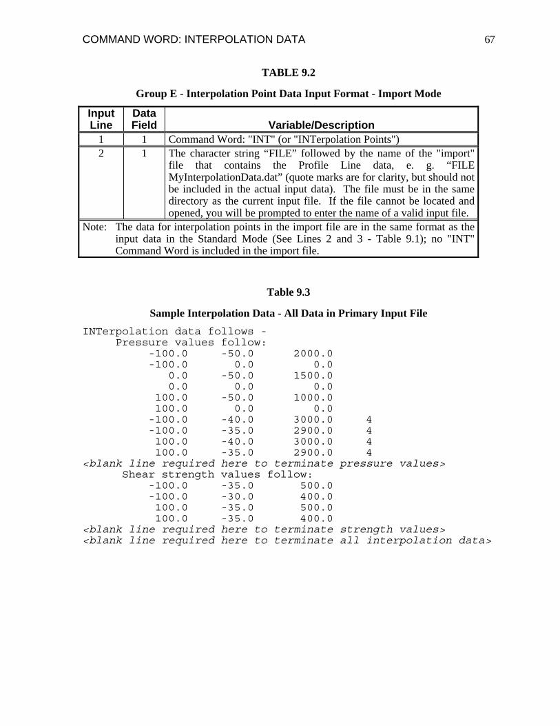
COMMAND WORD: INTERPOLATION DATA 67
TABLE 9.2
Group E - Interpolation Point Data Input Format - Import Mode
Input Line
Data Field
Variable/Description
1 1 Command Word: "INT" (or "INTerpolation Points") 2 1 The character string “FILE” followed by the name of the "import"
file that contains the Profile Line data, e. g. “FILE MyInterpolationData.dat” (quote marks are for clarity, but should not be included in the actual input data). The file must be in the same directory as the current input file. If the file cannot be located and opened, you will be prompted to enter the name of a valid input file.
Note: The data for interpolation points in the import file are in the same format as the input data in the Standard Mode (See Lines 2 and 3 - Table 9.1); no "INT" Command Word is included in the import file.
Table 9.3
Sample Interpolation Data - All Data in Primary Input File INTerpolation data follows - Pressure values follow: -100.0 -50.0 2000.0 -100.0 0.0 0.0 0.0 -50.0 1500.0 0.0 0.0 0.0 100.0 -50.0 1000.0 100.0 0.0 0.0 -100.0 -40.0 3000.0 4 -100.0 -35.0 2900.0 4 100.0 -40.0 3000.0 4 100.0 -35.0 2900.0 4 <blank line required here to terminate pressure values> Shear strength values follow: -100.0 -35.0 500.0 -100.0 -30.0 400.0 100.0 -35.0 500.0 100.0 -35.0 400.0 <blank line required here to terminate strength values> <blank line required here to terminate all interpolation data>

COMMAND WORD: INTERPOLATION DATA 68
Table 9.4
Sample Interpolation Data Using Import File - Primary Input File Contents
INTerpolation data follows - FILE MyInterpolationData.dat
Table 9.5
Sample Interpolation Data Using Import File - Import File Contents
Pressure values follow: -100.0 -50.0 2000.0 -100.0 0.0 0.0 0.0 -50.0 1500.0 0.0 0.0 0.0 100.0 -50.0 1000.0 100.0 0.0 0.0 -100.0 -40.0 3000.0 4 -100.0 -35.0 2900.0 4 100.0 -40.0 3000.0 4 100.0 -35.0 2900.0 4 <blank line required here to terminate pressure values> Shear strength values follow: -100.0 -35.0 500.0 -100.0 -30.0 400.0 100.0 -35.0 500.0 100.0 -35.0 400.0 <blank line required here to terminate strength values> <blank line required here to terminate all interpolation data>

COMMAND WORD: INTERPOLATION DATA 69
Figure 9.1 - Interpolation Data Points with Triangulation of Convex Hull
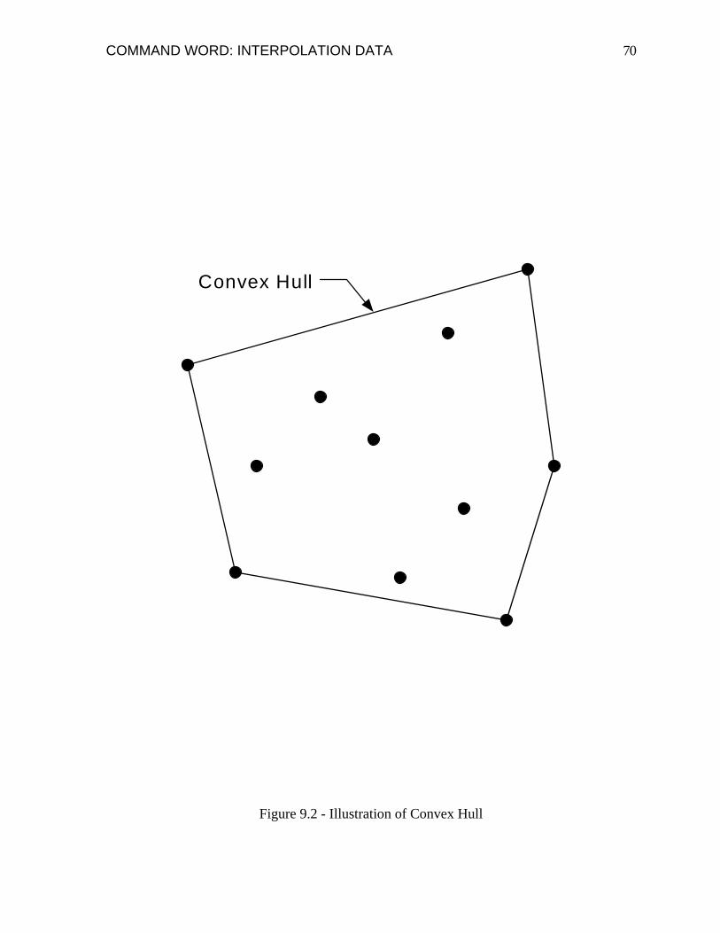
COMMAND WORD: INTERPOLATION DATA 70
Convex Hull
Figure 9.2 - Illustration of Convex Hull

COMMAND WORD: INTERPOLATION DATA 71
Figure 9.3 - Triangulation of Convex Hull Extending Beyond the Region of Materials That Contain the Interpolation Points.

COMMAND WORD: INTERPOLATION DATA 72
Figure 9.4 - Incomplete Data Points and Triangulation Causing Unsuccessful Interpolation.
COMMAND WORD: SLOPE GEOMETRY
73
Section 10 - GROUP F DATA FOR THE SLOPE GEOMETRY (Optional)
Introduction
Group F data are used to define the slope geometry when the geometry is different from the one defined by the Profile Lines. As discussed for the Profile Line data in Section 6, the slope geometry data allow you to "cut" several different slope geometries in a given soil profile (set of Profile Lines); any soil in the profile which lies above the surface defined by the slope geometry data is ignored. Several different slope geometries may be considered for the same set of Profile Lines by simply changing the slope geometry (Group F) data.
Once a slope geometry is defined, either by Profile Lines or Group F input data, the slope geometry remains in effect until new Group F data are specifically entered to change the slope geometry. You must enter Group F data even if new slope geometry are to be generated from a new set of Profile Line data. In this case when new geometry need to be generated you should enter the Group F data to "cancel" the existing slope geometry. To "cancel" the existing slope geometry you should enter a "null" set of slope geometry data as described later in this section.
Description of Data
The slope geometry data define the surface profile of the slope and consist of the coordinates of points from left-to-right along the surface of the slope. The points are assumed to be connected by straight lines to form a continuous slope profile. When the slope geometry is specified by the Group F data all material (soil, rock, etc.) above the surface of the slope is ignored. Thus, Profile Lines specified in Group B can define an original soil profile, and Group F slope geometry data can describe one or more slope profiles excavated into the original soil profile.
Both left and right facing slopes are allowed; a single set of slope geometry may contain both a left and a right face. Vertical "slopes" and horizontal "slopes" are also allowed. In the case of a horizontal "slope," distributed loads (See Group G data) are usually applied and the problem becomes essentially a bearing capacity problem1.
1 Although the problem is a bearing capacity problem, the factor of safety is still defined with respect to shear strength. Conventional analyses for bearing capacity generally define the factor of safety with respect to load. The two factors of safety are different; the factor of safety with respect to shear strength is usually as close or closer to unity as the factor of safety with respect to load. Depending on whether the factors of safety are less than or greater than unity, one value may be lower than the other and vice-versa.

COMMAND WORD: SLOPE GEOMETRY 74
Special Note for Flat Slopes
Special care is required when using UTEXAS4 with either very flat or horizontal "slopes". UTEXAS4 determines the direction (left or right) of potential sliding by comparing the elevations of the ground surface at the two ends of the shear surface. If the left end is higher than the right end, the direction of potential sliding is assumed to be to the right for the specific shear surface examined. Otherwise the direction of potential sliding is assumed to be to the left. For horizontal slopes the direction of sliding is assumed to be from right to left. Accordingly, for horizontal "slopes" shear surfaces should be directed to the left of the area of the applied surface loading. For flat, but not horizontal, slopes the direction of sliding is assumed to be in the direction in which gravity would produce sliding, i.e., from high to low. If sliding is possible and of interest for the opposite direction from gravity, due for example to relatively high surface pressures, a special "Opposite Sign Convention” option must be activated by entering optional data in the Group K - Analysis/Computation data (See Table 14.18). The direction of the slope face being analyzed is discussed further in Section 14.
Input Data Format
Group F data for the slope geometry must immediately follow the Command Word “SLO” (or “SLOPE”). The form of input for the slope geometry is presented in Table 10.1. Sample input data are presented in Table 10.2.
When a "null" set of slope geometry data is required to "cancel" the existing slope geometry and force UTEXAS4 to generate new slope geometry for a new set of Profile Lines, the Command Word "SLO" is entered and immediately followed by a blank line of data. This forces UTEXAS4 to discard any existing slope geometry data and new geometry will be computed from the current Profile Lines prior to performing the next slope stability computations. When slope data are "cancelled" the following message is written to the output file: "All slope data have been deleted ('cancelled') and will be re-generated.". This will be followed later by a table containing the new slope geometry data (assuming that there are no errors in the new Profile Line data).

COMMAND WORD: SLOPE GEOMETRY 75
TABLE 10.1
Group F – Slope Geometry Data Input Format
Input Line
Input Field
Variable/Description
1 1 Command Word: "SLO" (or "SLOPE”). 2 1 X coordinate of slope point. 2 2 Y coordinate of slope point.
Repeat Line(s) 2 for additional points defining the surface profile of the slope. Data for more than one point (2 quantities) may be entered on a given line of input data; however, each line of data must contain integer multiples of 2 quantities, comprising complete sets of data for slope points. Input a blank line to terminate the slope geometry data (all Group F data); then return to input of Command Words (Section 4).
TABLE 10.2
Sample Slope Geometry Data SLOpe geometry data follows – -100.00 -10.00 0.00 0.00 50.00 15.00 100.00 16.00 140.00 5.00 200.00 0.00 <blank line required here to terminate slope data>

COMMAND WORD: DISTRIBUTED LOADS
76
Section 11 - GROUP G DATA FOR DISTRIBUTED LOADS (Optional)
Introduction
Group G data are used to describe distributed loads1 (stresses, pressures) on the surface of the slope. Distributed loads are specified in terms of the components of stress acting normal (perpendicular) to the slope and tangential (parallel) to the slope.
Description of Data
Distributed loads are specified in the input data by a series of points along the surface of the slope from left to right. For each point the coordinates (x,y) and the values of the shear and normal stress are specified. The stresses are assumed to vary linearly between pairs of adjacent points. Pressures are assumed to be zero to the left of the first point specified and zero to the right of the last point specified. If an abrupt, “step” change in stress occurs at a point, data for two distributed load points with the same coordinate should be entered. The first such point designates the stresses to the immediate left of the point, while the second point designates the stresses to the right.
A series of distributed loads produced by water and an additional surcharge are illustrated in Fig. 11.1. Each point represents a point where the distributed load must be specified. The numbers beside each point indicate the sequence in which values must be entered. Two numbers are shown beside points where a "step" in the load exists and two values of load are specified at these locations.
The sign convention for normal stresses is that compression is positive; tension is negative. Shear stresses are positive when they act to the right and negative when they act to the left.
Distributed loads can be specified on any portion of the slope, including vertical segments2. When distributed loads are specified for vertical segments of a slope a “left-to-right” sequence is interpreted as the sequence that would be encountered if one moved along the surface of the slope from left to right. Thus, for a vertical segment of the slope that faces to the left, lower points on the segment will be specified before higher points. Similarly for a 1 Distributed loads were referred to as “Surface Pressures” in UTEXAS2 and UTEXAS3. 2 This is different from versions previous to UTEXAS4, which did not permit distributed loads (“surface pressures”) to be specified on vertical slopes.

COMMAND WORD: DISTRIBUTED LOADS 77
vertical segment that faces to the right, higher points on the segment will be specified before lower points.
The coordinates of points which are input to define the distributed loads should be specified as precisely on the surface of the slope as is practically possible. If the points do not coincide with the surface of the slope an error condition may result and computations will be abandoned with an appropriate error message.
Automatic Generation of Distributed Load Data
When distributed loads are produced entirely by water above the surface of the slope, the data for the distributed loads can automatically be created by UTEXAS4. In order for UTEXAS4 to create the distributed load data you must first enter a piezometric line (See Group D data) to represent the water surface that produces the loads. If water levels vary, e. g. between the upstream and downstream slopes of a dam, the piezometric line can change elevation accordingly between the points where the water intersects the upstream and downstream faces of the slope. Once the piezometric line is defined, you must direct UTEXAS4 to compute distributed loads from the piezometric line by entering Group G data in the special format described in Table 11.2. The piezometric line that is entered for computing distributed loads may or may not also be used to define pore water pressures in materials via the Group C Material Property data. Use of the piezometric line for pore water pressures in this case is optional.
In some cases only a portion of the distributed loads may be due to surface water. If this is the case, you can still use UTEXAS4’s ability to compute distributed loads as follows: First run UTEXAS4 with instructions to compute distributed loads from an appropriate piezometric line representing the surface water conditions, but terminate computation of the factor of safety (via the “NO compute” Sub-Command Word described for the Group K data). Then, use the computed surface loads as a starting point to manually create an appropriate set of distributed load input data. This may be particularly useful for slopes with very complex, irregular surface geometries.
Multi-Stage Computations
When two-stage or three-stage computations are being performed, separate sets of distributed loads are specified for the first and subsequent (second & third) stages. Values specified for the first stage are not used for the second and third stage and vice-versa.
COMMAND WORD: DISTRIBUTED LOADS 78
Input Data Format
Distributed load data must immediately follow the Command Word "DIS" (or "DISTRIBUTED LOADS"). Data may either be entered for each point or the data may be computed using a previously defined piezometric line and slope geometry. The appropriate formats for data entry are presented in Tables 11.1 and 11.2, respectively. Sample distributed load data are presented in Table 11.3. The sample data correspond to the distributed loads illustrated in Fig. 11.1.

COMMAND WORD: DISTRIBUTED LOADS 79
TABLE 11.1
Group G - Distributed Load Data Input Format for Individual Points
Input Line
Input Field Variable/Description
1 1 Command Word: "DIS" (or "DISTRIBUTED LOADS"). 2 1 X coordinate of point where distributed load value is to be specified. 2 2 Y coordinate of point where distributed load value is to be specified. 2 3 Normal stress acting perpendicular to the surface of the slope at the
designated point. 2 4 Shear stress acting parallel (tangential) to the surface of the slope at the
designated point. Repeat Line(s) 2 for additional points to define the distributed loads in a left-to-right sequence. More than one set of data (4 quantities) may be entered on a given line; however, each line must contain integer multiples of 4 quantities, comprising complete data sets. Input a blank line to terminate the distributed load data (all Group G data); then return to input of Command Words (Section 4).
TABLE 11.2
Group G - Distributed Load Data Input Format for Automatic Computation of Pressures from a Piezometric Line
Input Line
Input Field
Variable/Description
1 1 Command Word: "DIS" (or "DIStributed loads. 2 1 Number of the piezometric line that is to be used to compute the
distributed loads.
Note: UTEXAS4 distinguishes between which input format is used (Table 11.1 or Table 11.2) based on the number of values entered on the first line of data immediately following the Command Word. If four values, or integer multiples of four values are entered on the second line of data (first line after Command Word), the format in Table 11.1 is assumed; If a single value is entered, the format in Table 11.2 is assumed and the distributed loads are generated automatically from the designated piezometric line.

COMMAND WORD: DISTRIBUTED LOADS 80
Table 11.3
Sample Distributed Load Data DIStributed load data follows – 0.0 0.0 936.0 0.0 7.5 0.0 936.0 0.0 15.0 5.0 624.0 0.0 20.0 5.0 624.0 0.0 20.0 15.0 0.0 0.0 25.0 20.0 0.0 0.0 25.0 20.0 500.0 0.0 30.0 20.0 500.0 0.0 30.0 20.0 1000.0 0.0 35.0 20.0 1000.0 0.0 35.0 20.0 500.0 0.0 40.0 20.0 500.0 0.0 40.0 20.0 0.0 0.0 45.0 15.0 0.0 0.0 45.0 5.0 624.0 0.0 55.0 0.0 936.0 0.0 62.5 0.0 936.0 0.0 <blank line required here to terminate distributed load data>

COMMAND WORD: DISTRIBUTED LOADS 81
1000 psf
500 psf 500 psf
10 feet
Scale
1 2
3 4
5
6,7
8,9 10,11
12,13
14
15
16 17
1, 2, etc.- Indicates point where distributed loads must be specified
Figure 11.1 - Illustration of Distributed Loads Showing Locations Where Values Must be Specified in the Input Data.

COMMAND WORD: LINE LOADS
82
Section 12 - GROUP H DATA FOR LINE LOADS (Optional)
Introduction
Group H data are used to describe “line” loads1. Line loads are assumed to be extend infinitely far in the direction perpendicular to the two-dimensional cross-section of the slope represented in the analysis; they appear as “point” loads when viewed in the two-dimensions of the slope cross-section (Fig. 12.1). Line loads may act either on the surface of the slope or internally, beneath the surface.
Description of Input Data
For each line load the coordinates of the point where the load acts in the two-dimensional plane of the slope and the value of the load are specified as input data. The load represents the load per unit distance (feet, meter, etc.) in the direction perpendicular to the two-dimensional plane of the slope. Load values can be entered as data in two forms:
(1) The separate horizontal (x) and vertical (y) components of the line load force are specified.
(2) The magnitude of the line load and its inclination from the horizontal are specified.
If the components of the force are specified, positive values are considered to act to the right and upward (in the direction of positive values of the coordinates). If the magnitude and inclination of the force is specified, the magnitude is generally specified as positive. The direction is then specified as an angle measured from the horizontal and considered to be positive in the counter-clockwise direction. Negative angles are assumed to be clockwise from the horizontal direction. If the magnitude of the force is positive and the angle is zero degrees (0°), the force acts horizontally to the right. If the angle is ± 180° and the force is positive, the force acts to the left. If the force is positive and the angle is 90° the force acts vertically upward. If the angle is - 90° (or + 270°) a positive force acts vertically downward. Directions and sign convention for the inclination of positive forces is shown in Fig. 12.2,
1 Line loads were previously referred to as “Concentrated Forces” in UTEXAS2 and UTEXAS3.

COMMAND WORD: LINE LOADS 83
The preferred way of specifying forces by their magnitude and inclination is to specify a positive value for the magnitude of the force and an appropriate positive or negative value for the inclination of the force. However, for each positive value of force, there is an equivalent negative value acting in the opposite direction that can be specified. Negative values for the force correspond to a force acting in the direction opposite to the directions described for positive forces. Thus, a positive force acting at an inclination of 0° is identical to a negative force of the same magnitude acting at ±180°. Either positive or negative forces and directions are admissible. (See examples in Fig. 12.3).
Line loads can be specified anywhere on or inside the slope. There is actually no illegal location, although loads specified entirely outside the slope are ignored in the computations. During computation UTEXAS4 checks to determine if any line load is located within any slice. If it is, the force is added to the other forces acting on that slice. If a line load lies outside the limits of all slices, it is ignored for the particular shear surface where this occurs.
Multi-Stage Computations
When two-stage or three-stage computations are performed, separate sets of line loads are specified for the first and the subsequent (second & third) stages. Line loads specified for the first stage are not used for the second and third stage and vice-versa.
Input Data Format
Line load (Group H) data must immediately follow the Command Word “LIN” (or “LINE LOADS”). The form of input for the Line Loads is presented in Table 12.1. Sample line load data are presented in Table 12.2.
Line loads are numbered for reference purposes; any sequence of unique positive integer values ranging from 1 to 2,147,483,647 may be used. Once a set of line loads has been entered and some computations have been performed, individual line loads may be altered and new computations may be performed. To alter line loads new data are simply entered for selected loads. The new data should identify the load by reference to the number assigned in the original input data, and the new data will then replace the old data for each particular line load number that is re-entered..

COMMAND WORD: LINE LOADS 84
TABLE 12.1
Group H - Line Load Data Input Format
Input Line
Input Field Variable/Description
1 1 Command Word: "LIN" (or "LINE LOADS").. 2 1 Number used to identify the line load currently being specified on this
line of data. 2 2 X coordinate of point where line load acts. 2 3 Y coordinate of point where line load acts. 2 4 Depending on the option designated in Field 6 on this line of data, enter
a value for one of the following: Horizontal force component of the line load (Option = 1) /OR/ Magnitude of the resultant force (Option = 2).
2 5 Depending on the option designated in Field 6 on this line of data, enter a value for one of the following: Vertical force component of the line load (Option = 1) /OR/ Inclination of the force, measured in degrees from the horizontal (Option = 2).
2 6 An integer designating how the force due to the line load is described (in Fields 4 & 5), as follows: = 1: If the horizontal and vertical components of the force are specified.= 2: If the magnitude and direction (inclination) of the resultant force
are specified Repeat Line(s) 2 for additional line loads. Data for more than one line load (6 quantities) may be entered on a given line of input data; however, each line of data must contain integer multiples of 6 quantities, comprising complete sets of data for each line load. Input a blank line to terminate the line load data (all Group H data); then return to input of Command Words (Section 4).
TABLE 12.2
Sample Line Load Data LINe load data follows – 1 20.0 40.0 0.0 -5000.0 1 2 40.0 45.0 5000.0 -90.0 2 <blank line required here to terminate line load data>

COMMAND WORD: LINE LOADS 85
(a) Oblique View
(b) Two-Dimensional View
Figure 12.1 - Oblique and Two-Dimensional Views of a Line Load.

COMMAND WORD: LINE LOADS 86
+ θ
(a) Positive Line Load with Positive Inclination
- θ
(b) Positive Line Load with Negative Inclination
Figure 12.2 - Illustration of Direction and Corresponding Sign Convention for Inclination of Positive Values of Line Loads
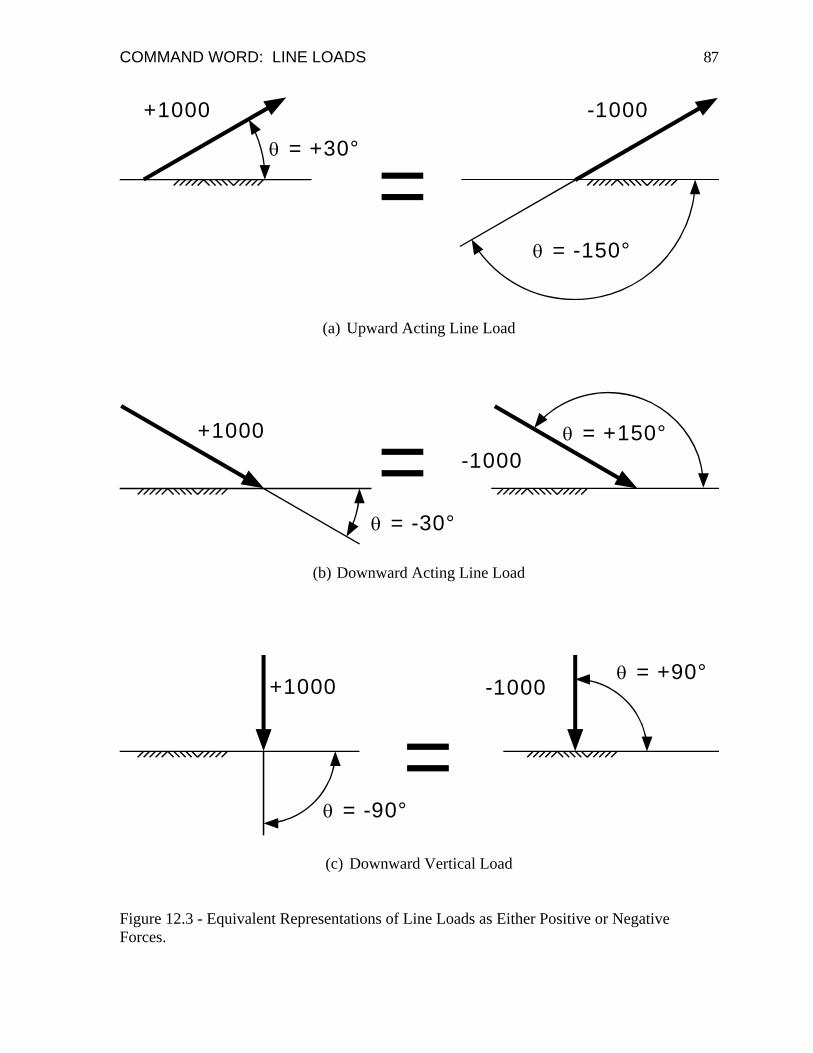
COMMAND WORD: LINE LOADS 87
θ = +30°
+1000
θ = -150°
-1000
=
(a) Upward Acting Line Load
+1000-1000
θ = -30°
θ = +150°=
(b) Downward Acting Line Load
=+1000 -1000
θ = -90°
θ = +90°
(c) Downward Vertical Load
Figure 12.3 - Equivalent Representations of Line Loads as Either Positive or Negative Forces.

COMMAND WORD: REINFORCEMENT
88
Section 13 - GROUP J DATA FOR INTERNAL REINFORCEMENT (Optional)
Introduction
Group J data are used to specify reinforcing elements in the slope. Reinforcing elements may represent geo-grids, geotextles, piles, micro-piles, piers, tie-back anchors, nails or metallic strips. The reinforcement is represented as a series of one or more lines; each line is continuous and piecewise linear. The lines are defined in the input data by specifying coordinates along the lines similar to the way that soil profile lines are entered. At each coordinate point the longitudinal and transverse forces in the reinforcement are also specified. The forces are assumed to vary linearly between points. Reinforcement is considered to only produce internal forces in the soil; Reinforcement has no weight and does not occupy any physical space in the cross-section; it is assumed to be infinitesimally thin.
Longitudinal forces in the reinforcement are considered to be positive when they are tensile; compressive forces are considered to be negative. Shear forces are considered to be positive when they act such that they produce a counter-clockwise moment on the adjoining reinforcement and soil mass as shown in Fig. 13.11.
Representation and Use in Computations
UTEXAS4 uses the reinforcement data to compute forces acting on the soil above the shear (sliding) surface. When the base of a particular slice interscts a reinforcement line, a force is calculated and applied as a known force to the base of the slice. This force is considered to be a force transmitted through the reinforcement in addition to forces transmitted through the soil. Other, separate shear and normal forces on the base of the slice (S and N, respectively) are used to represent forces transmitted through the soil. The orientation of the reinforcement force is determined both by the orientation of the reinforcement and an angle, Δψ , representing a maximum rotation (reorientation) of the reinforcement due to deformation. The reorientation angle, Δψmax, represents the angle that the reinforcement force is rotated through from its initial direction. If the angle is specified as zero (0.0), the reinforcement forces are assumed to be oriented in accord with the original direction(s) of the reinforcement, i. e. parallel to and perpendicular to the direction of the reinforcement for the longitudinal and transverse forces, respectively. If the angle, Δψmax, is
max
1 The sign convention for shear forces is opposite to the sign convention used for shear forces in UTEXAS3. The sign convention was changed to conform with the more conventional practice used in structural mechanics and structural engineering.

COMMAND WORD: REINFORCEMENT 89
greater than zero, the reinforcement is assumed to be rotated through the specified angle, but not past the point where the reinforcement would become tangent to the shear surface. The direction that the reinforcement is assumed to rotate depends on the direction that the slope faces, as shown in Fig. 13.2. The directions of rotation shown in Fig. 13.2 represent positive rotations (Δψmax), negative rotations are in the opposite directions. For horizontal ground, the rotation is assumed to be the same as that for a left-facing slope, i. e. counter-clockwise rotation of the reinforcement is considered to be positive.
Reinforcement forces are represented in the stability computations in one of the following two ways, which may be chosen and designated in the input data:
(1) Reinforcement forces are calculated and applied to the base of the slice(s) that the reinforcement intersects and to the boundaries between each slice that the reinforcement intersects (See Fig. 13.3).
(2) Reinforcement forces are applied only to the base of the slice that the reinforcement intersects (See Fig. 13.4).
When reinforcement forces are applied to the boundaries between slices (Fig. 13.3) the forces are calculated at the point where the reinforcement crosses the slice boundary. Equal and opposite forces are applied to adjacent slices on each side of a given boundary. The system of forces shown in Figs. 13.3 and 13.4 are both statically correct and differ only in how the reinforcement forces are distributed among slices.
The way that reinforcement forces are applied is designated in the input data for each reinforcement line by a “Reinforcement Force Option”. The Reinforcement Force Option designates whether forces are applied both internally and on the base of the slice (Option 1 - Fig. 13.3) or only to the base of the slice (Option 2 - Fig. 13.4). In general Option 1 is believed to be a more realistic representation of how reinforcement forces are distributed to the soil; Option 1 is the default value used by UTEXAS4 unless Option 2 is specified.
Depending on how reinforcement forces are applied, the side forces between slices have different meanings. If reinforcement forces are applied between slices (Option 1), the side forces represent only the forces transmitted directly through the soil. If reinforcement forces are applied only to the base of the slices (Option 2), the side forces represent the forces in the soil, plus the reinforcement forces. This has implications for the side force inclinations in the procedures of slices used to calculate the factor of safety, regardless of whether the side force inclination is specified in the input data or calculated as an unknown. For example in Spencer’s procedure the side forces are all assumed to have the same inclination (side forces are parallel). This means that if Option 1 is used, only the soil forces are parallel; the reinforcement forces between slices will act at the orientations stipulated for the reinforcement forces. In contrast, when Option 2 is used the resultant side forces due to the reinforcement and soil forces combined are parallel (have the same inclination). Likewise, if a force equilibrium procedure is used, the side force inclination that is specified is the

COMMAND WORD: REINFORCEMENT 90
inclination of the soil forces only if Option 1 is used, and the inclination of the combined soil and reinforcement forces if Option 2 is used. Experience to date (1998) indicates that there is little difference between results obtained using Option 1 and Option 2; however, this may not always be the case.
Selection and Interpretation of Forces for Input
The full reinforcement forces specified for the reinforcement are applied to slices to compute the factor of safety. The factor of safety that is subsequently computed is the factor of safety applied to soil strength, not to the reinforcement forces. Accordingly, any factor of safety that needs to be applied to the reinforcement should be applied to reduce the reinforcement forces before they are entered in the input data. The factor of safety should include allowances for such factors as creep, corrosion, decay, and construction damage. In addition, the factor of safety may need to reflect what deformations are tolerable; the reinforcement forces may need to be reduced to maintain acceptable deformations. For piles and piers, the forces will typically be less that the shear resistance of the structural members, because of limitations on bending stresses under lateral loads. Due to the wide variety of reinforcing materials and the various patterns in which reinforcing is installed, this manual does not attempt to give any guidelines on selection of reinforcement forces for particular situations.
The limit equilibrium procedures employed in UTEXAS4 assume a two-dimensional cross-section of infinite extent in the direction perpendicular to the plane of the cross-section. Reinforcement forces should represent the force per unit distance perpendicular to the two dimensional cross-section. Thus, for finite width reinforcement, e. g. piles, piers, nails, etc., the force that is input does not represent the force per reinforcing element, but rather the equivalent force per unit distance. Forces for any such finite reinforcement should be calculated and entered as forces per unit distance.
Input Data Format
Group J data must immediately follow the Command Word "REI" (or "REINFORCEMENT LINES"). The data input is described in Table 13.1. Sample input data are presented in table 13.2.
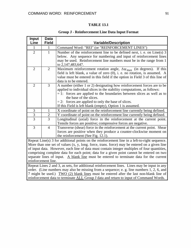
COMMAND WORD: REINFORCEMENT 91
TABLE 13.1
Group J - Reinforcement Line Data Input Format
Input Line
Data Field
Variable/Description
1 1 Command Word: "REI" (or "REINFORCEMENT LINES") 2 1 Number of the reinforcement line to be defined next, i. e. on Line(s) 3
below. Any sequence for numbering and input of reinforcement lines may be used. Reinforcement line numbers must be in the range from 1 to 2,147,483,647.
2 2 Maximum reinforcement rotation angle, Δψmax (in degrees). If this field is left blank, a value of zero (0), i. e. no rotation, is assumed. A value must be entered in this field if the option in Field 3 of this line of data is to be entered.
2 3 A number (either 1 or 2) designating how reinforcement forces are to be applied to individual slices in the stability computations, as follows: = 1: forces are applied to the boundaries between slices as well as to
the base of the slices. = 2: forces are applied to only the base of slices. If this Field is left blank (empty), Option 1 is assumed.
3 1 X coordinate of point on the reinforcement line currently being defined. 3 2 Y coordinate of point on the reinforcement line currently being defined. 3 3 Longitudinal (axial) force in the reinforcement at the current point.
Tensile forces are positive; compressive forces are negative. 3 4 Transverse (shear) force in the reinforcement at the current point. Shear
forces are positive when they produce a counter-clockwise moment on the reinforcement (See Fig. 12.1).
Repeat Line(s) 3 for additional points on the reinforcement line in a left-to-right sequence. More than one set of values (x, y, long. force, trans. force) may be entered on a given line of input data. However, each line of data must contain integer multiples of four quantities, comprising complete data for each point; data for a given point cannot be entered on two separate lines of input. A blank line must be entered to terminate data for the current reinforcement line. Repeat Lines 2 and 3, as sets, for additional reinforcement lines. Lines may be input in any order. (Line numbers may also be missing from a sequence; e. g. line numbers 1, 2, 6, and 7 might be used.) TWO (2) blank lines must be entered after the last non-blank line of reinforcement data to terminate ALL Group J data and return to input of Command Words.

COMMAND WORD: REINFORCEMENT 92
TABLE 13.2
Sample Reinforcement Line Input Data REInforcement line data follow - 1 0.0 1 0.0 25.0 5000.0 0.0 40.0 5.0 5000.0 0.0 50.0 0.0 0.0 0.0 <blank line required here to complete data for 1st line> 2 0.0 1 0.0 10.0 7500.0 0.0 40.0 -10.0 7500.0 0.0 50.0 -15.0 0.0 0.0 <blank line required here to complete data for 2nd line> 3 0.0 2 20.0 50.0 0.0 0.0 20.0 40.0 0.0 0.0 20.0 20.0 0.0 15000.0 20.0 -10.0 0.0 15000.0 20.0 -15.0 0.0 0.0 20.0 -25.0 0.0 0.0 <blank line required here to complete data for 3rd line> 4 15.0 1 0.0 17.5 0.0 0.0 5.0 17.5 1000.0 0.0 30.0 17.5 1000.0 0.0 40.0 17.5 0.0 0.0 <blank line required here to complete data for 4th line> <blank line required here to terminate all reinforcement data>

COMMAND WORD: REINFORCEMENT 93
Figure 13.1 - Direction for Positive Shear Forces in Reinforcement
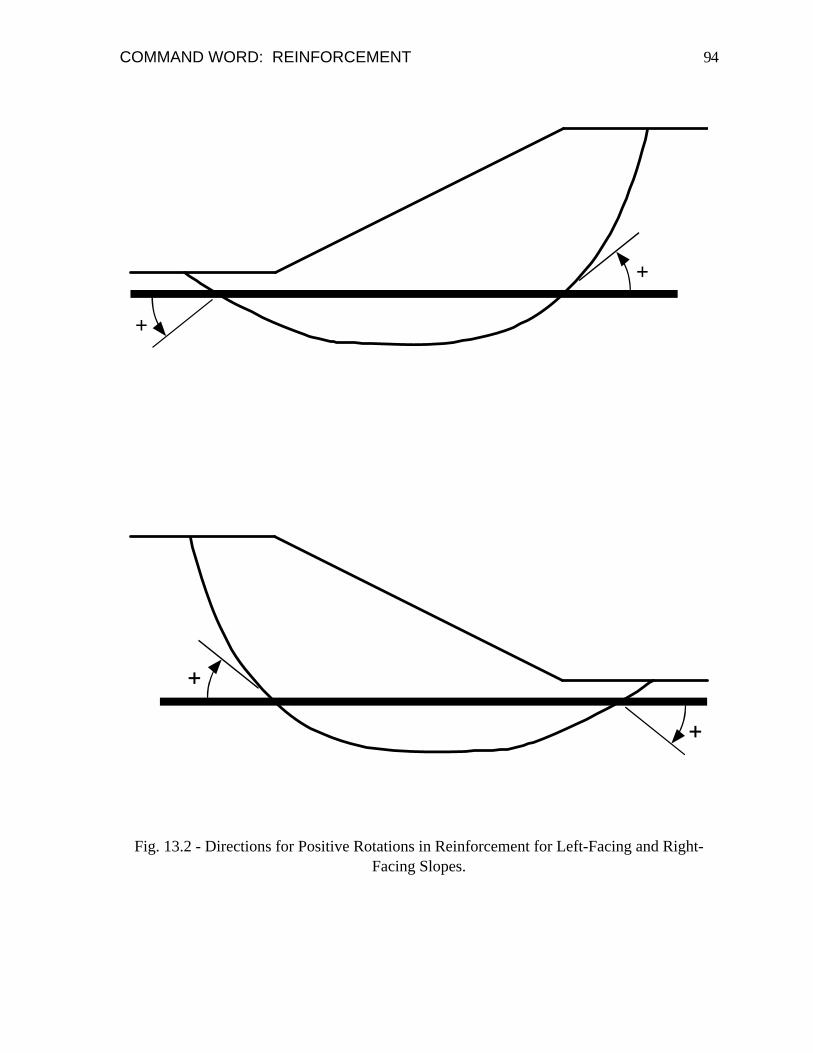
COMMAND WORD: REINFORCEMENT 94
+
+
Fig. 13.2 - Directions for Positive Rotations in Reinforcement for Left-Facing and Right-Facing Slopes.

COMMAND WORD: REINFORCEMENT 95
Fig. 13.3 - Reinforcement Forces Applied to Slices When Option = 1.

COMMAND WORD: REINFORCEMENT 96
Fig. 13.4 - Reinforcement Force Applied to Slice When Option = 2.

COMMAND WORD: ANALYSIS/COMPUTATION
97
Section 14 - GROUP K DATA FOR THE ANALYSIS AND COMPUTATIONS
Introduction
The Group K input data designate whether the shear surface is circular or noncircular and whether computations are to be performed for a single, specified shear surface or an automatic search is to be performed to locate a critical shear surface with a minimum factor of safety. The Group K Data also include information for a tension crack, seismic loads (seismic coefficient), information on how the shear surface is subdivided into slices, and parameters that control the iterative solution for the factor of safety and an automatic search. These data are described in this section.
The Group K data are entered in two parts. The first part consists of the data that define the shape of the shear surface and appropriate information on the location of either the individually selected shear surface or the initial trial shear surface to be used for a search. These data are described in Table 14.1 and Tables 14.2a through 14.2e. The second part of the Group K data consist of a series of one or more optional Sub-Command "Words" that are used to designate various options for the analysis. The Sub-Command Words are summarized in Table 14.3. Each Sub-Command Word may or may not require additional data immediately following the Sub-Command Word. Details of the Sub-Command Words are given in Tables 14.4 through 14.29. Table 14.3 includes cross-references to tables where more detailed information is given for each Sub-Command Word.
Individually Specified Shear Surfaces
UTEXAS4 allows you to specify individual shear surfaces, one-by-one, and the factor of safety is computed for each surface (automatic searches are described in a later section). The individual shear surfaces may be either circular or noncircular. Also, they may be for either the left or the right face of the slope and the computations are performed accordingly. Numerous shear surfaces may be specified, including a mixture of both circular and noncircular shear surfaces and for both the left and right faces of the slope. The input formats for individual circular and noncircular shear surfaces are different. The input for circular of noncircular shear surfaces is described separately in the two sections below.

COMMAND WORD: ANALYSIS/COMPUTATION 98
Individual Circular Shear Surfaces
The location of a circular shear surface is designated by the coordinates of the center of the circle and the radius of the circle. The x and y coordinates of the center of the circle are specified as input data. The radius either may be specified directly as input data or may be specified indirectly and calculated by UTEXAS4 in one of the following two ways:
(1) The shear surface may be designated as passing through a given point and the coordinates of the point are specified,
(2) The shear surface may be designated as being tangent to a given "tangent line" and the line is input; the tangent line may be either a horizontal line or a piecewise linear line with inclined as well as horizontal segments.
UTEXAS4 automatically subdivides the soil above the (circular) shear surface into vertical slices using one of the following two methods, which you can select:
Option 1. The soil is subdivided so that the angle (Δθ) which is subtended by radii extended to each side of the base of the slice does not exceed a certain, designated value, Δθmax (Fig. 14.1). In most cases many of the slices which are actually created will have a base which subtends an angle of less than the prescribed angle (Δθmax) because of other constraints. For example, when the bottom of a slice would otherwise cross a boundary between two materials, a smaller slice width is used to ensure that the base of the slice lies in only one material.
Option 2. The soil is subdivided so that the arc length ( Δ ) along the base of each slice does not exceed a certain, designated value, Δ xma (Fig. 14.1). As in Option 1, the actual arc length will be less than the value of Δ max for slices where other constraints dictate a narrower slice.
The first option (Option 1) is the default option; slices are created using a constant subtended angle of 3 degrees. You can enter another value for the subtended angle or select the alternate option of a constant arc length ( Δ max ) if you wish. This is done with the optional Sub-Command Words (See Tables 14.5 and 14.26). If either of the options and corresponding values of Δθmax or Δ max produces more than the maximum number of slices allowed by UTEXAS4, the specified values (Δθmax, Δ max ) are successively doubled until no more than the allowable maximum results.
The maximum number of slices is contained in the UTEXAS4 Application Settings described in Section 2. This number is ordinarily set as 100, which seems to be adequate for almost all practical problems. However, if the soil profile is very complex and a large number of points are used for the Profile Lines, the required number of slices can be large and exceed 100. If this happens, it may be necessary to increase the maximum number of slices in the UTEXAS4 Application Settings (See Section 2).

COMMAND WORD: ANALYSIS/COMPUTATION 99
Individual Noncircular (including Wedge) Shear Surfaces
The location of an individual noncircular shear surface is defined by entering the x-y coordinates of selected points along the shear surface. The specified points are assumed to be connected by straight lines; vertical segments are not allowed. UTEXAS4 requires that specific points on the shear surface be defined. For example the points where the shear surface crosses a Profile Line must be defined. However, these required points do not need to be included in the input data; any additional coordinates needed by UTEXAS4 will be computed and added to the coordinates that you input.
In specifying the end points for noncircular shear surfaces be careful to specify the end points as nearly on the surface of the slope as practically possible. If the specified end points do not lie precisely on the slope, UTEXAS4 adjusts the coordinates so that they are located on the slope. This is done by determining the intersection of the shear surface with the surface of the slope and then changing the coordinates of the end point to those of the intersection point. However, the first two or last two end points on a shear surface must never both lie above the surface of the slope or an error condition will result.
When a vertical "tension" crack is specified, as described later, the end point on the shear surface at the end near the crack ("upslope" end) is adjusted so that the end point coincides with the bottom of the crack. If the end point is specified on the surface of the slope and a crack exists, the end point is automatically adjusted so that it is at the bottom of the crack. The position of the new end point is calculated by determining where the first segment of the shear surface (at the upslope end) intersects the a line representing the bottom of the crack. However, if the first two end points on the shear surface both lie above the bottom of the crack an error condition will exist and UTEXAS4 will not be able to adjust the end point.
Vertical slice boundaries are located at each point specified on the shear surface as well as at additional points required by UTEXAS4 (e. g. where the shear surface crosses a Profile Line). Additional slices are added by further subdividing the shear surface into slices using one of the following two criteria; the criteria can be selected as part of the input data:
Option 1. The soil mass is subdivided so that the length of the base of each slice (chord length) does not exceed a specified maximum value, . To accomplish this UTEXAS4 first computes the coordinates which are required for other purposes, such as where the shear surface crosses a boundary between different soils, and adds these required coordinates to the coordinates which were entered as input data. The distance between each pair of adjacent points is then checked. If the distance exceeds the prescribed distance,
Δ max
Δ max , the segment of the shear surface between the pair of points is divided into enough equal length increments so that the required maximum slice base length is no longer exceeded.

COMMAND WORD: ANALYSIS/COMPUTATION 100
Option 2. The soil mass is subdivided to produce an approximate minimum number of slices, referred to as nnominal. In this case UTEXAS4 divides the (chord) distance between the first and last point on the shear surface, by nnominal, to obtain a distance, Δ . This distance (Δ ) is then applied as a maximum slice base length equivalent to in the same manner as described for the Option 1 above. Δ max
Initially the second option (Option 2) is used as the default. Slices are created using a minimum number of slices, nnominal; thirty (30) is used as the minimum number of slices. If you desire, either a different minimum number of slices, nnominal, or a different maximum slice base length, , may be entered as input data. This is done with the optional data entered using the appropriate Sub-Command words (See Tables 14.6 and 14.12). If either of the selected options and corresponding values of the parameters
Δ max
Δ max and nnominal results in more than the maximum number of slices allowed, the value of nnominal will be halved or the value of will be doubled until a small enough number of slices results. The maximum number of slices allowed is contained in the UTEXAS4 Application Settings (See Section 2).
Δ max
Vertical ("Tension") Cracks
A vertical, "tension" crack can also be specified as part of the input data for each shear surface (Fig. 14.2). Slices are terminated at the location of the crack and soil above the portion of shear surface that lies upslope of the crack is ignored in the stability calculations. Except for any forces produced by water in the crack (see below), the crack boundary is assumed to be stress free.
A crack may be specified in terms of either the depth of the crack or the elevation of the bottom of the crack (Table 14.8). Also the depth or elevation for the crack may be either constant or variable. If the depth or elevation is variable, depths or elevations are specified at selected lateral positions (x) along the slope; depths or elevations are assumed to vary linearly between points where values are specified.
You specify the information needed to define the depth of the crack; UTEXAS4 then determines the actual location of the crack for each shear surface depending on the crack depth profile and the position of the shear surface. The crack is assumed to be located at the point where the shear surface first reaches the crack depth near the upslope (crest rather than toe) portion of the shear surface as illustrated for three circles in Figure 14.3. No crack is assumed unless crack data are specifically entered as input.
In addition to specifying a crack, you may specify that the crack contains water or some other fluid. The presence of water in the crack is specified in the input data either by the depth of the water or the elevation of the water surface in the crack. The water depth or elevation may be either constant or variable. When the water depth or surface elevation is variable, the depth or elevation is specified at selected lateral positions (x) along the slope. The data for water in the crack are also optional and are entered with the supplemental data

COMMAND WORD: ANALYSIS/COMPUTATION 101
described later (See Table 14.29). No water is assumed if none of the optional data for crack water is entered.
You may also specify the unit weight of the water or other fluid in the crack, w crack− ; otherwise a default value is assumed for the unit weight of fluid in the crack. Water in a crack is considered to produce a horizontal force in the crack equivalent to the force produced by hydrostatic pressures acting over the depth of water specified. However,
γ
water in the crack is not considered to produce any pore water pressures in the soil; pore water pressures must be specified separately by means of other input data (e.g., piezometric lines).
Assumed Direction of Sliding and Slope Face Analyzed
Ordinarily the slope face and direction of sliding for the computations are determined by comparing the elevations of the ground surface at each end of the shear surface. If the ground surface at the right end of the shear surface is higher than the left end, the left face of the slope is assumed and the shear stresses along the shear surface are assumed to act from left to right. Similarly, if the left end is higher than the right end the shear stresses act from right to left. The direction assumed for the shear stresses for left and right facing slopes is illustrated in Fig. 14.4. In the case of a horizontal ground surface, the right end of the shear surface is assumed to be the upslope end of the shear surface, i.e. a horizontal ground surface is treated like a left-facing slope, and the crack is located near the right, rather than left end of the shear surface as shown in Fig. 14.5.
There are two cases where the methods described above for determining the slope face and direction of sliding require special considerations. These are described further below.
Special Case 1
For some slopes a given circle may intersect both left-facing and right-facing portions of a slope (Fig. 14.6). If the extreme left and right intersection points are at the same elevation the slope is assumed to be left facing and the right-most segment of the shear surface is analyzed. You can change this convention by use of the Sub-Command Words "RIG" (Right) and "LEF" (Left), which override the normal convention used to determine which face of the slope is to be analyzed. These Sub-Command Words are described in Table 14.14.
Special Case 2
In some cases it may not be appropriate to determine the direction of sliding based on the elevations of the two end points of the shear surface. For example, for the circle shown in Fig. 14.7 the end points at the right are higher than the end point at the left and a left-facing slope would be assumed with the shear stress acting in the direction indicated in 14.7a.

COMMAND WORD: ANALYSIS/COMPUTATION 102
However, if there are distributed loads and the distributed loads are high enough that a lower factor of safety exists for sliding "upslope" with the shear stress acting in the direction shown in part (b) of this figure, UTEXAS4 will not automatically recognize this. In order to force the shear stresses to act in the opposite direction from what would normally be assumed based on the geometry, UTEXAS4 has an "Opposite Sign Convention" option that can be activated by the Sub-Command Word "OPP" (See Table 14.18). The Opposite Sign Convention option can also be used for a horizontal ground surface to force the direction of sliding to be opposite to the one normally assumed (Fig. 14.8).
The distinction between the Sub-Command Words "LEF" and "RIG" designating the slope face to be analyzed and the Sub-Command Word "OPP" designating the "Opposite Sign Convention" is important. The Sub-Command Words "LEF" & "RIG" designate the slope face to be analyzed; depending on the slope face chosen the shear stresses act as shown in Fig. 14.4. The other Sub-Command Word ("OPP") modifies the direction of the shear stress once the slope face (left or right) is chosen.
Automatic Searches
Automatic searches may be performed with either circular or noncircular shear surfaces. The automatic search procedures used by UTEXAS4 are designed to assist you in locating the most critical shear surface corresponding to a minimum factor of safety. However, care and judgement must be exercised in using the automatic search procedures to ensure that the most critical shear surface has actually been located. Careful judgement is especially important when more than one "local" minimum exists. The search procedures for circular or noncircular shear surfaces are described separately below.
Circular Shear Surfaces
Two different search schemes are available for circles. The first search scheme for circles (Type 1) employs a "floating" grid whose size and spacing between points changes as the search progresses. This scheme is very efficient and generally more effective for finding a critical circle than the second scheme. The floating grid procedure has been used for a number of years and is the procedure used in the predecessors to UTEXAS4 (SSTAB1, UTEXAS, UTEXAS2, and UTEXAS3).
The second search scheme for circles (Type 2) uses a "fixed" grid where the spacing between grid points and the overall location of the grid remain fixed. This grid is useful for drawing contours of factor of safety for various center point locations. It is not as efficient as the first search scheme and may require repeated runs to eventually find a critical circle; however, the scheme is useful when contours of factor of safety are required. The second search scheme is a relatively new implementation and has not been used as extensively as the first scheme. For many problems both search schemes may be used to arrive at a final solution. The two search schemes are described further below.

COMMAND WORD: ANALYSIS/COMPUTATION 103
Type 1 – “Floating Grid” Search Scheme.
In an automatic search with the “floating grid” UTEXAS4 systematically varies the center point location using a 3 x 3, square 9-point grid. The center point of the first grid used is specified in the input data and should represent a best estimate of the x and y coordinates of the center of the critical circle. The initial spacing between points in the 9-point grid is thirty (30) times a specified minimum grid spacing, δg−min. . The minimum grid spacing,
, is entered as input data and may be considered to be the approximate accuracy with which the center of the critical circle is to be eventually determined. δg−min.
The location of the center point of the square grid is shifted during the search until the center of the grid corresponds to the center of a circle with a lower factor of safety than any of the circles with centers at the eight surrounding grid points on the perimeter of the grid. The 9-point grid is always shifted such that the center of the new grid is located at the point where the lowest factor of safety was calculated with the previous grid. The spacing between grid points is also changed during the automatic search. The spacing is reduced from an initial spacing which is 30 times a specified minimum grid spacing, to spacings of 5, 3 and, finally, 1 times the specified minimum grid spacing. Computed values for the factor of safety are stored in memory, and in most cases values are only calculated for circles where values have not been previously computed. The search is terminated when the grid spacing has been reduced to the specified minimum spacing ( δg− ) and the center of the 9-point grid has the lowest factor of safety of the nine grid points.
min.
Experience with the "floating grid" search scheme has shown that specified minimum grid spacings ranging from one percent to ten percent of the slope height work well for locating the critical circle. However, the actual grid spacing used should be selected based on each individual problem to ensure that a critical circle is found. The distance should not exceed the thickness or smallest dimension of the smallest zone of soil which may influence the computed minimum factor of safety and critical shear surface.
To locate a critical circle with the floating grid the search alternates among a sequence of “modes” that define the radii of circles for each grid point. Three different “modes” are used to define the radius for a given center:
Mode 1 - Circles pass through a given point; the coordinates of the point are specified.
Mode 2 - Circles are tangent to a given “tangent” line; the location of the tangent line is specified. The tangent line may either be a horizontal line or an irregular, piecewise linear continuous line specified by a series of points along the line.
Mode 3 - Circles have a given, constant radius, which is specified as part of the input data.

COMMAND WORD: ANALYSIS/COMPUTATION 104
By successively varying the three available modes of search and for each mode finding a critical center (by moving the “floating grid”), an overall critical circle can be found. The sequence of steps for doing this is described below:
Step 1: A critical circle is first located by varying the center point locations and using an “initial mode” (specified as input data) to define the radius for each center. The “initial mode” may be either Mode 1, 2 or 3 although Modes 1 and 2 are generally recommended for the initial mode. If Mode 1 is selected, the x and y coordinates of the point through which the circles pass are specified. If Mode 2 is selected, the location of the tangent line is specified. If Mode 3 is selected, the radius is specified.
Step 2: Once the center of a critical circle (minimum factor of safety) is located using the initial mode, the mode is changed. If the initial mode was Mode 1 or Mode 3, the mode is changed to Mode 2, and a horizontal tangent line is defined at the elevation of the bottom of the critical circle which was located using the previous mode (Modes 1 or 3). The horizontal tangent line is then used to define the radii of the subsequent circles tried. If Mode 2 is specified for the initial search, the mode is changed to Mode 3, and the radius of the critical circle from Mode 2 is adopted for the search. Once a new mode is defined a new critical circle is located by again moving the "floating" grid.. If the difference between the values of the factor of safety for the two critical circles, located using the modes of Step 1 and Step 2, is less than 0.001, the critical circle is considered to be the most critical circle located in Step 2, and the search is completed. However, if the factor of safety changes by more than 0.001 for successive modes, the search continues to Step 3.
Step 3: After Step 2, the mode used to define the radii alternates between Mode 2 (tangent line) and Mode 3 (constant radius). If the initial mode was Mode 2 and the tangent line was not horizontal, the tangent lines used subsequently in Step 3 will have the same shape as the initial tangent line, but be displaced vertically. For each mode (2 or 3) the floating grid is used to search for the center of a circle giving a minimum factor of safety. This process is continued until the difference between the values of the minimum factors of safety for the critical circles found with successive modes is less than 0.001. Mode 1 is never used after Step 1; Mode 1 may only be used for the initial mode of search.
UTEXAS4 allows you to terminate the search after Step 1 is completed if you wish (See Table 14.9 - Sub-Command Word "STO"). Thus, you may find the critical circle through a designated point, tangent to some line, or with a given radius and, then, terminate the search. You can repeatedly start new searches with different initial modes and in this way exercise stricter control over the pattern of search.

COMMAND WORD: ANALYSIS/COMPUTATION 105
Limiting Depth for Circles
When locating the overall critical circle it is sometimes desirable to impose a limiting depth below which the critical circle cannot pass. This may be achieved either by specifying a stratum of soil at the selected limiting depth and assigning a high shear strength to the particular stratum or by specifying an appropriate limiting elevation, ylimit, below which the critical circle is not allowed to pass. The limiting y elevation (ylimit) is specified in the data input for the search as described in Table 14.2c (Input Line 2 - Data Field 4).
Limiting Lowest Elevation for Centers
It is also sometimes useful to limit the lowest elevation allowed for center points tried during a search. To do this you should enter a value for the variable, ylowest center, as described in Table 14.2c (Input Line 2 - Data Field 5).
Multiple Minima/Local Minima
In some cases it will be possible to find several local "critical" circles with local minimum factors of safety. The center of each such locally critical circle will be surrounded by center points having higher values for the factor of safety. In such cases, when a given search is performed, only one of the locally critical circles will be searched-out and located; the circle so found may not be the one with the absolute, lowest value for the factor of safety. In order to locate the circle with the absolute, lowest value for the factor of safety, several automatic searches will need to be performed using different starting points for the circles and, perhaps, different initial modes for the search. You will then need to compare the values of the factor of safety for each of the "critical" circles located by these independently started searches to determine the actual minimum factor of safety and the location of the overall critical circle. This requires you to specify several sets of Group K data for a given problem.
Subdivision into Slices
For automatic searches the same procedures are used for subdividing the circle into slices as described earlier for individual circular shear surfaces. Similarly, a vertical ("tension") crack may be specified and the crack may be designated to contain water or some other fluid, as described earlier for individually specified shear surfaces.
Maximum Attempts
In each “mode” of search with the 9-Point grid, UTEXAS4 will attempt calculations with as many as 50 trial grids (nominally 450 grid points) before abandoning a search. This number of grids (50) has generally been found to be more than sufficient for finding a critical circle within the tolerances normally used. The critical circle is usually found and the search proceeds after much fewer grids have been used. However, if the limit is reached and more

COMMAND WORD: ANALYSIS/COMPUTATION 106
trial grids are needed the maximum number of grids can be increased from the default value of 50 (See Table 14.27).
Type 2 – “Fixed Grid” Search Scheme.
The second type of automatic search for circular shear surfaces uses a “fixed” grid with points in the grid representing the centers of circles. Normally the grid is a quadrilateral grid defined by four corner points; the location of the four corner points is prescribed in the input data and is not varied during the search. The numbers of points along each pair of opposing sides of the grid is also designated in the input data. "Grid points" are then defined by subdividing opposing sides into increments and connecting the subdivsion points by straight lines. The intersections of the two series of straight lines from opposing sides then define the grid points.
As a special, alternative the "grid" may simply consist of a straight line defined by two end points. Grid points then correspond to points spaced uniformly along the line connecting the two end points.
Regardless of whether the grid is a quadrilateral or a straight line, the radii of circles centered at each grid point are varied until a critical radius, producing the lowest factor of safety for that center point is found. This process is repeated for each center point in the grid.
To find the "critical" radius the radius for each center point in the grid is varied between maximum and minimum values that are specified by the input data. The maximum and minimum radii are determined based on one or more criterion for the radii; the following criteria may be specified:
(1) A point through which the circles pass,
(2) A specific value of radius,
(3) A “tangent” line to which circles are tangent - the “tangent” line may either be a horizontal line or an irregular, piece-wise linear line described by a series of points along the line.
Several of the above criteria may be specified. For example, 3 different points through which circles pass, 2 values of radius and 2 tangent lines may all be specified. Then, for each center point UTEXAS4 will calculate the radii corresponding to each criterion; the maximum and minimum values calculated are used to define the maximum and minimum radii for that center point. The specific criteria that govern the maximum and minimum radii for each center point may differ from center point to center point, depending on the location of the center point. For example, one center point might be located so that the maximum and minimum radii are governed by a point and a specified value of radius. Another center point might be located so that the maximum and minimum radii are governed by two tangent lines

COMMAND WORD: ANALYSIS/COMPUTATION 107
that were specified. Consequently the maximum and minimum radii for each center point may be different for each center point.
For each center point in the grid the radii are varied between the maximum and minimum values by first subdividing the range (maximum radius minus minimum radius) into a specified number of increments, e. g. ten increments, might be used. The number of increments into which the radii are divided for the search is specified in the input data (See Table 14.2d – Input Line 4, Data Field 2). Once the radii have been varied by the appropriate increments, the factors of safety for each radius are examined to determine where apparent minima may exist, i. e. where the factors of safety for adjacent values of radii were higher (Fig. 14.9). Any intervals where it appears that a minimum may exist are then further subdivided and the radii are incremented in the interval to seek further refinement of the minimum. The intervals are successively reduced in size until the increment in radius is less than a prescribed minimum increment. The minimum increment to be used is specified as a distance in the input data (See Table 14.2d – Line 4). In some cases the initial subdivision and refinement of radii in an interval where a minimum appears to exist may reveal more than one minimum once the radius increment is reduced (Fig. 14.10). Whenever this occurs both of the sub-intervals where minima appear to exist will be further subdivided to find each “local” minimum.
For each grid point all of the radii attempted and the corresponding factors of safety are output. Ordinarily, the radii and factor of safety are sorted and output in the order of increasing radius. As an option the values can be output in the actual order that the radii were incremented and tried (See Table 14.25). Regardless of the order values are output for each grid point, the radius producing the overall lowest factor of safety as well as other radii producing local minimum factors of safety for each grid point are identified on the output. Finally, after completion of the calculations for all grid points, the circle having the lowest factor of safety is identified and output again.
Lateral Restrictions on Search.
Ordinarily there are no restrictions on the lateral extent of shear surfaces that will be attempted during an automatic search other than restrictions that may be inherent and imposed by the geometry and material properties. However, in special cases it may be desirable to restrict shear surfaces to only a particular zone of interest. For example it might be necessary to restrict the extent of a search using circles if only the lower portion of a slope like the one shown in Fig. 14.11 is to be analyzed. UTEXAS4 allows you to restrict the extent of the search with circular shear surfaces by entering special restriction data (See Table 14.21). The search restriction data allow you to specify restriction limits either in terms of absolute x coordinates or in terms of lateral extents relative to the center of the circle. The limits may also stipulate that either all of the shear surface must lie within the limits or only some of the shear surface must lie within the limits. Examples of circles

COMMAND WORD: ANALYSIS/COMPUTATION 108
satisfying and not satisfying each type of limit are shown in Figs. 14.12 and 14.13 for restrictions specified in terms of absolute and relative distances, respectively.
Noncircular Shear Surfaces (Including Wedge)
The search for a critical noncircular shear surface is performed using a search based on the procedure developed by Duncan and Celestino (1981). The shear surface is systematically moved from an initial (starting) position, until a minimum factor of safety is calculated. You must assume the initial position of the shear surface. The location of the initial shear surface is specified in the input data by entering coordinates of points along the shear surface (from left to right), much as an individual shear surface is specified when no search is performed. The initial position should represent your best estimate for the location of the critical shear surface. In most cases it is useful to perform first a search using circles to judge where to start the search with noncircular shear surfaces. Also, if a slope contains a thin seam of particularly weak material, through which the critical shear surface is expected to pass, the initial shear surface should be selected so that it passes through the weaker material.
You may choose to have each of the coordinate points you specify for the initial shear surface either move during the search or remain fixed at their initial position. In most cases all points will be allowed to move. As the first step in an automatic search, each moveable point on the shear surface is moved an incremental distance (specified by the input data) in each of two opposite directions (e.g., up and down). The movement of points on the shear surface is done in two steps:
Step 1: Points defining the noncircular shear surface are shifted one by one on a TEMPORARY basis and a factor of safety is calculated as each individual point is shifted to its temporary location. When any one point is shifted, all other points are left at their original (initial) positions; no points are permanently moved during the first step of the automatic search. Each point is shifted in two opposing directions. End points on the shear surface are shifted along the slope, or along the bottom of the vertical "tension" crack, when a crack is specified and the end point is at the crack. You have no control over the direction of shifting the two end points of the shear surface. For other points you may specify the direction in which each point is shifted, or UTEXAS4 will automatically compute a direction for shifting each point. When UTEXAS4 computes a direction for shifting each point, the direction is approximately normal (perpendicular) to the shear surface; the direction may, thus, change somewhat as the shear surface moves.
Step 2: Once each point on the shear surface has been shifted and the factor of safety has been computed for each shift, a new estimate for the position of the most critical shear surface is made and the initial shear surface is PERMANENTLY moved. The new estimate for the position of the shear surface is made using the procedure of

COMMAND WORD: ANALYSIS/COMPUTATION 109
Celestino and Duncan (1981); the factor of safety is assumed to vary parabolically with the position of the shear surface.
Completion of these two steps constitutes what is referred to as a single "pass." Once the new estimate of position for the shear surface is made and the surface is moved ("pass" is completed) a new pass is initiated: Each point on the shear surface is again shifted in the manner used for the first step and the process is repeated to find yet another estimate for the critical shear surface.
The distance each point is temporarily shifted to compute the factor of safety is determined based on an "initial incremental shift distance" ( Δ i ), which is specified by input data. Initially the points will be shifted a distance equal to the specified distance ( Δ i ). UTEXAS4 will automatically reduce the distance shifted as the distance that the shear surface is permanently moved (as opposed to temporarily shifted) on each "pass" diminishes. (The actual distance the shear surface is permanently moved on each step is computed by UTEXAS4.) The distance the shear surface is shifted is reduced from its initial value ( Δ i ) by successively halving the value until a specified minimum, final value ( ) is reached and no further, significant changes are occurring in the factor of safety
fΔ1.
In most procedures of limit equilibrium slope stability analysis the equilibrium equations used to compute the factor of safety will begin to yield unrealistic values for the stresses near the toe of shear surfaces when the shear surface slopes upward at angles much steeper than those which would be expected based on considerations of passive earth pressure. During a search trial shear surfaces can potentially become excessively steep unless some restriction is placed on the amount the shear surface is shifted during the trial-and-error search. UTEXAS4 permits you to specify a maximum steepness, αmax. , that is allowed for the "toe" portion of the shear surface. The "toe" portion is considered to be any portion of the shear surface which is inclined upward in a direction opposite to the slope face. The maximum steepness allowed is specified by a value for the optional parameter αmax. in the input data for the noncircular shear surface. (A default value of 50 degrees is assumed if no value is input).
Judgement and some trial and error may be required to select an optimum value for the incremental shift distance, . Experience to date indicates that relatively large distances may be used provided that the limiting steepness (
Δ iαmax. ) described above is not in excess of
50 degrees (the default value). The value specified for the terminal distance for shifting, fΔ , should generally be no more than 10 to 25 percent of the thickness of the thinnest stratum through which the critical shear surface may pass. For example, if the thinnest stratum is 5 1 Stopping of the search is based on two criteria: If the distance for shifting points has reached the minimum value and the factor of safety did not change when the surface was shifted on the last "pass", the search is completed. Otherwise, if the distance for shifting points has reached the minimum value and the largest rate of change in factor if safety with position (s) of the shear surface, dF/ds, is less than 0.001/Δi, the search is completed. The position, s, is measured in the direction that points on the shear surface are moved. The rate of change in factor of safety (dF/ds) is computed by taking the first derivative of the assumed parabolic relationship between factor of safety and position of the shear surface. The largest rate of change/derivative (dF/dS), considering all points on the shear surface, is used in determining when the search is completed.

COMMAND WORD: ANALYSIS/COMPUTATION 110
feet thick, and an acceptable degree of resolution for the critical shear surface is 20 percent of the thickness of a stratum, the minimum value for shifting the shear surface would be specified as 1 foot (0.2 x 5 feet).
UTEXAS4 will attempt as many as 50 “passes” in which points are moved on the noncircular shear surface before abandoning a search. This maximum number of passes (50) has generally been found to be adequate for finding a shear surface that produces a minimum factor of safety within prescribed tolerances. If the number of passes is reached before a suitable minimum is found the maximum number of passes permitted can be changed from 50 to a larger value (See Table 14.19).
“N-Most” Critical Shear Surfaces
UTEXAS4 permits you to retain the results for a selected number of the most critical shear surfaces (lowest factors of safety) and print a summary of the location of the shear surfaces along with the corresponding factors of safety once the search is completed. The shear surfaces that are "saved" may also be displayed later using the companion graphics program (TexGraf4). The number, “n”, of shear surfaces retained is designated in the input data; if no number is input, no shear surfaces are retained. The number of shear surfaces is entered as optional data using the Sub-Command Word “SAV” (See Table 14.22.)
When the “n-most” critical shear surfaces are saved they are also written to the Graphics Exchange file if one is written. They can then be displayed using the companion graphics program, TexGraf4.
Seismic Coefficient
"Pseudo-static" analyses can be performed where a horizontal body force is applied to each slice to simulate earthquake loading. This is accomplished using a single seismic coefficient (K) by which the weight of each slice is multiplied to obtain additional, horizontal body forces. The seismic force on each slice may act at one of the following three possible locations which are designated in the input data for UTEXAS4:
(1) Center of gravity of slice.
(2) Mid-height of slice.
(3) Bottom of slice (at shear surface).
The center of gravity and mid-height of the slice may correspond to the same point, but also can differ if the unit weight of soil varies over the height of the slice. A positive seismic

COMMAND WORD: ANALYSIS/COMPUTATION 111
coefficient corresponds to a force acting to the left for the left face of a slope and to the right for the right face of a slope.
The seismic coefficient is specified as part of the Group K data (See Table 14.23). UTEXAS4 assumes that there are no seismic forces (default) unless a seismic coefficient is input; however, once a value is input it remains in effect either until another value, including zero, is input with Group K data or asterisks ("***") are encountered in the Command Words. No special treatment is given to shear strengths when a seismic coefficient is used; the shear strengths are defined and interpreted in the normal manner as described in Section 6. The only effect which a seismic coefficient has on the computations is to produce an added, horizontal body force on each slice.
When conventional, single-stage computations are performed, the seismic coefficient is applied for the first stage. When multi-stage computations are performed, the seismic coefficient is not applied for the first stage computations; instead, it is applied for the second and third stage computations only.
Generally analyses with a seismic coefficient should be performed using two-stage computations. The shear strength used for the second stage should depend on the effective stresses that the soil is consolidated to before the earthquake. The shear strengths should also reflect any loss in strength due to earthquake shaking.
Computation for Factor of Safety
You may select the procedure of slices used to compute the factor of safety; however, Spencer's procedure is strongly recommended. Spencer's procedure is the default procedure used by UTEXAS4 unless you specifically designate otherwise. The procedures available in UTEXAS4 are briefly described below followed by a discussion of input parameters.
Procedures for Computing F
Four procedures are available for computing the factor of safety. The procedures are: (1) Spencer's procedure, (2) the Simplified Bishop procedure, (3) the Corps of Engineers' Modified Swedish procedure, and (4) Lowe and Karafiath's procedure. The Simplified Bishop procedure is restricted to computations with circular shear surfaces while the other procedures may all be used with either circular or noncircular shear surfaces. Attempts to use the Simplified Bishop procedure for noncircular shear surfaces will result in an error condition and computations will not be attempted.
Spencer's Procedure.
In Spencer's procedure all side forces are assumed to have the same inclination and all requirements for static equilibrium are satisfied. The trial and error solution of the

COMMAND WORD: ANALYSIS/COMPUTATION 112
equilibrium equations involves successive assumptions for the factor of safety and side force inclination until both force and moment equilibrium are satisfied. Once the factor of safety and side force inclination are found the following additional unknowns are calculated: (1) Normal forces, N, on the base of each slice, (2) resultant side forces, Z, between slices, and (3) location of the side forces, y - the "line of thrust" (Fig. 14.14a) t
Simplified Bishop Procedure.
The side forces are assumed to act horizontally in the Simplified Bishop procedure. Thus, there are no shear forces on the vertical boundaries between slices. Equilibrium of forces in the vertical direction is satisfied for each slice and equilibrium of moments about the center point of the circle is satisfied for the entire soil mass (all slices combined). The trial and error solution for the factor of safety involves successive assumptions for the factor of safety until the moment equilibrium equation is satisfied (vertical force equilibrium is implicitly satisfied). Once the factor of safety is found the normal forces, N, on the base of the slices are calculated (Fig. 14.14b)
Corps of Engineers' Modified Swedish Procedure.
In the Modified Swedish Procedure all side forces are assumed to have the same inclination (are parallel) and the inclination is assumed by the user. According to Corps of Engineers (1970) the inclination is assumed to be equal to the "average slope of the embankment;" however, other, often flatter, inclinations are sometimes assumed in practice. The Modified Swedish procedure satisfies equilibrium of forces in both the vertical and horizontal directions for individual slices, but does not satisfy moment equilibrium. The procedure has been found to sometimes overestimate the factor of safety by as much as 50 percent or more and the results are sometimes very sensitive to the assumed inclination for the side forces. The trial and error solution for the factor of safety involves successive assumptions for the factor of safety until equilibrium of forces is satisfied. Once the factor of safety is calculated, the unknown normal forces, N, on the base of each slice and the resultant side forces, Z, between slices are calculated (Fig. 14.14c).
The so-called "Simplified Janbu" procedure is a procedure of slices that assumes the side forces are horizontal and satisfies force equilibrium, but not moment equilibrium. It is identical to the Corps of Engineers' Modified Swedish Procedure if the side force inclination is assumed to be zero, i. e. horizontal, in the Corps of Engineers' procedure. Accordingly, calculations can be performed by the Simplified Janbu procedure as a special case of the Corps of Engineers' Modified Swedish procedure1.
1 The Simplified Janbu procedure usually tends to underestimate the factor of safety. The procedure is not recommended, but is discussed here for reference and possible use in checking results of others who may have used the procedure.

COMMAND WORD: ANALYSIS/COMPUTATION 113
Lowe and Karafiath's Procedure.
Lowe and Karafiath's procedure is identical to the Corps of Engineers' Modified Swedish Procedure except for the assumed inclinations of the side forces. In Lowe and Karafiath's procedure the side forces are assumed to be inclined at the average slope of the ground (slope) surface directly above and the shear surface directly below each vertical slice boundary. Thus, the side force inclinations generally vary from slice-to-slice. (In UTEXAS4 side force inclinations are computed by averaging "slopes," dy/dx, rather than angles.) The trial and error solution for the factor of safety in Lowe and Karafiath's procedure is identical to the one for the Modified Swedish procedure. Once a factor of safety has been calculated from the equilibrium equations, the same unknown that are calculated in the Corps of Engineers' Modified Swedish procedure are calculated in Lowe and Karafiath's procedure.
The "Unknowns"
All of the procedures used to compute the factor of safety in UTEXAS4 involve the calculation of other "unknowns" in addition to the factor of safety. This was indicated for each of the procedures above. The unknowns are illustrated in Fig. 14.14. In addition to the unknowns shown in Fig. 14.14 each of the procedures involve calculating the shear forces, S, on the base of the slices. The shear forces are not shown as unknowns, because they are known once the "unknowns", including the factor of safety, are found. The shear forces are related to the known and unknown values through the definition of the factor of safety. When the shear strengths are expressed using total stresses the shear forces (S) are calculated from the equation:
SF
=c N+Δ tan φ 14.1
where, c and φ are the respective Mohr-Coulomb cohesion and friction, N is the total normal force on the base of the slice, and Δ is the length of the base of the slice. When shear strengths are defined using effective stresses the shear force is computed from,
S c N uF
=+ −Δ Δa f tan φ 14.2
where c and φ are the respective Mohr-Coulomb cohesion and friction for effective stresses, u is the pore water pressure, and the other terms are the same as those in Eq. 14.1. All of the unknowns, including the shear forces are calculated and output by UTEXAS4. The normal forces (N) and shear forces (S) are actually output as stresses, by dividing the values of force by the respective area (Δ ) of the base of each slice

COMMAND WORD: ANALYSIS/COMPUTATION 114
Solution Parameters
All of the procedures for computing the factor of safety involve an iterative solution in which successive values are assumed for the factor of safety (and side force inclination in the case of Spencer's procedure), until one or more equilibrium equations are satisfied. The iterative solutions involve a number of "solution" parameters. Default values are assumed for the "solution" parameters with one exception: You must select and input as data a value for the side force inclination used in the Corps of Engineers' Modified Swedish procedure; a default value is not assumed. Default values are discussed later below.
The iterative solution for the factor of safety is initiated with initial trial values for the factor of safety, F0 (and side force inclination, θ0, in the case of Spencer's procedure). The trial values are then changed by successive approximations until all of the following conditions are satisfied, i.e. the solution converges:
1. Static equilibrium is satisfied within acceptable limits of accuracy. These limits are defined in terms of an "allowed" force imbalance, Fimbal, , and moment imbalance Mimbal. The specific imbalance limits which are satisfied depend on the procedure being used to compute the factor of safety (Spencer, Simplified Bishop, etc.)
2. The value of the factor of safety changes by no more than 0.00001 on successive iterations. In the case of Spencer's procedure the side force inclination must also not change by more than 0.0001 radians (≈ 0.006 degrees) on successive iterations.
If either of the above two conditions for convergence is not attained within a prescribed maximum number of iterations Imax, computations for the particular shear surface are abandoned and the next shear surface is considered.
The initial trial values for the factor of safety and side force inclination, F0 and θ0, respectively are assigned default values of 3.0 and 0.3 radians (approximately 17 degrees). The force and moment imbalances (Fimbal and Mimbal), and the allowable number of iterations (Imax) are assigned default values based on information in the UTEXAS4 Application Settings (See Section 2). Default values in the Application Settings depend on the current type of units; the default type of units is also set in the Application Settings and can be changed with the Command Words described in Section 4. You may also change the default values in the Application Settings as described in Section 2. You may change any one or all of the values for the solution parameters (Fimbal, Mimbal, F0, θ0 and Imax) through selective input of data. Several important features of the iterative solution for the factor of safety and side force inclination as well as the variables F0, θ0, Fimbal, Mimbal, and Imax are discussed further below.

COMMAND WORD: ANALYSIS/COMPUTATION 115
Factor of Safety.
The value of the factor of safety is permitted to change only by a maximum of five-tenths (0.5) on successive iterations. This constraint is placed on the solution to assist convergence. However, because of the limit on how much the factor of safety can change on consecutive iterations, if a very inaccurate estimate is made and specified for the initial value of the factor of safety (F0), the correct value may not be reached within the prescribed maximum number of iterations and the solution will fail to converge. Similar problems with convergence may develop when an automatic search is being performed and a trial shear surface passes through a zone of very high shear strength, such as concrete or a firm (rock) stratum, which has been specified for the purpose of limiting the extent of the critical shear surface. In this case a relatively large value for the factor of safety will be sought, but probably the value will not be reached within the allowed number of iterations. Thus, an indication will be given on the printed output that the solution did not converge. This problem of the solution not converging when the factor of safety is very large for one of the trial shear surfaces attempted is normally not of practical consequence. You should simply verify that, for the shear surfaces where the solution did not converge, the values for the factor are relatively large.
In addition to the constraint described above for the change in the factor of safety on successive iterations (0.5), the value of the factor of safety is not permitted to become less than one-tenth (0.10). While this constraint should be of little practical consequence, the solution will be terminated when the value for the factor of safety reaches a value of one-tenth.
A considerable amount of experience has shown that the numerical solution for the factor of safety and side force inclination is better conditioned and more likely to converge when the initial trial value for the factor of safety overestimates, rather than underestimates, the correct value. In many cases by simply increasing the initial estimate for the factor of safety (F0) the solution can be made to converge, where otherwise convergence was not achieved.
Side Force Inclination (Spencer's Procedure).
In Spencer's procedure the inclination of the resultant side forces between slices is assumed to be the same for all slices and is calculated along with the factor of safety as part of the iterative solution. An initial trial value is assumed for the side force inclination; the assumed value can be overridden by optional data if necessary (See Table 14.24). The initial trial value for the side force inclination is positive when the side force is inclined in the same direction as the slope, i. e. counter-clockwise from the horizontal for a left-facing slope and clockwise from horizontal for a right-facing slope (Fig. 14.15). Side forces with negative inclinations are inclined in directions opposite to the inclination of the slope.

COMMAND WORD: ANALYSIS/COMPUTATION 116
During the actual stability computations a different sign convention from the one described in the preceding paragraph is used for the side force inclination: Side force inclinations are considered to be positive when the side forces are inclined counter-clockwise from the horizontal regardless of the direction that the slope faces (Fig. 14.16), i.e. positive side forces correspond to a positive value for the slope, dy/dx, of the side forces. The sign convention shown in Fig. 14.16 is consistent with the sign convention used internally for the coordinates and other angles in UTEXAS4. All side force inclinations shown in the computed output use the sign convention shown in Fig. 14.16. The reason that the sign convention for input (Fig. 14.15) is different from the one used internally for computation (Fig. 14.16) is to allow you to enter a single value of side force inclination in the input data that will be applicable to both left- and right- facing slopes.
In the iterative solution procedure, the value of the side force inclination is not permitted to change by more than 0.15 radians (approximately 8.6 degrees) on successive iterations and will be adjusted accordingly when this limit is reached. In addition, the side force is not permitted to reach an inclination steeper than either +80 degrees for a left facing slope or -80 degrees for a right facing slope (Fig. 14.17). If these limits are reached, the iterative solution is terminated and an appropriate message is issued. Side force inclinations of less than -10 degrees for a left facing slope and greater than +10 for a right facing slope are also not allowed and will cause the solution to be terminated with an appropriate message (Fig. 14.17).
Side Force Inclination (Modified Swedish Procedure).
In the Corps of Engineers' Modified Swedish procedure the inclination of the side forces is assumed by the user. The inclination is input to UTEXAS4 as an angle, in degrees, measured from the horizontal plane. The sign convention used for the angle that is entered is the same as the one used for input of the initial trial side force inclination in Spencer's procedure (Fig. 14.15). Similarly, the sign convention used internally for computations and for output is the one shown in Fig. 14.16.
Allowed Force and Moment Imbalance.
The force and moment imbalances, Fimbal and Mimbal, respectively, are used as one of the criteria for convergence noted earlier. Depending on the specific procedure being used to compute the factor of safety the solution must satisfy force equilibrium (Modified Swedish procedure, Lowe and Karafiath procedure), moment equilibrium (Simplified Bishop), or both force and moment equilibrium (Spencer's procedure) within specified tolerances ("imbalances"). The Simplified Bishop procedure also satisfies force equilibrium in the vertical direction; however, it satisfies force equilibrium exactly and, thus, the imbalance should always be zero.
The values for the allowable force and moment imbalance may not be zero, because round-off error and the use of a finite number of significant figures by the computer usually

COMMAND WORD: ANALYSIS/COMPUTATION 117
prevent computation of precisely zero values for verifying convergence. Experience up to mid-1998 with prior versions of the UTEXAS software, which use essentially the same algorithms used in UTEXAS4, has shown that for many slopes, the value of the factor of safety is computed to within a minimum of four significant figures (0.01 percent) of the exact solution using default force and moment imbalances of 100 pounds and 100 foot-pounds, respectively.
Allowable force and moment imbalances may be specified as part of the input data to override the default values. When you specify values in the input data you can specify values either in terms of absolute values of force and moment or as decimal fractions of the force and moments produced by the weight of soil above the shear surface. The input of force and moment imbalances is described in Tables 14.11 and 14.17, respectively.
Iteration Limit.
The maximum number of iterations allowed for the iterative solution for the factor of safety is contained in the UTEXAS4 Application Settings (See Section 2). When reasonable values are assumed for the initial trial values of the factor of safety and side force inclination, convergence to a solution is normally attained within from three to ten iterations, provided that the factor of safety is estimated to within ± 1.5 of the correct value and, in the case of Spencer's procedure, that the side force inclination is estimated to within ± 20 degrees of the correct value. If the solution fails to converge within the allowable number of iterations, you can increase the number of iterations either by changing the UTEXAS4 Application Settings or by entering the maximum number of iterations as part of the input data (See Table 14.13). Increasing the number of iterations may help in some cases, but in other cases it may not.
Minimum Weight
UTEXAS4 automatically rejects shear surfaces where the total weight of soil above the shear surface is less than a certain amount. It is particularly important that the designated force and moment imbalances for convergence be some small fraction of the forces and moments produced by the weight of the soil and other known forces. By limiting the weight of soil that will be considered you can better insure that the force and moment imbalances will not be an appreciable fraction of the total forces and moments acting on the soil mass.
The options for defining the minimum weight required before shear surfaces are rejected depend on how the force and moment imbalances (Fimbal and Mimbal) are prescribed. If actual values of force and moment imbalance are stipulated (rather than a fraction of the total weight and moment due to the soil), the minimum weight can be set in either of two ways:
1. A minimum weight can be stipulated (either in the UTEXAS4 Application Settings or directly as input data).

COMMAND WORD: ANALYSIS/COMPUTATION 118
2. If the minimum weight has been stipulated to be zero, the minimum weight automatically will be set equal to 1000 times the prescribed force imbalance. i. e. the prescribed, allowable force imbalance is 0.001 times the minimum weight allowed.
The data entry format for the minimum weight is presented in Table 14.16.
When the allowable force or moment imbalances are specified as decimal fractions of the weight and the moment produced by the weight, respectively, the minimum weight for computations must be designated as non-zero. The minimum weight is initially set by the values in the UTEXAS4 Application Settings (See Section 2) and may be reset by entering a value as input (See Table 14.16).
Special Note for Automatic Searches
During an automatic search some efficiency may be realized by changing the initial trial values for the factor of safety (and side force inclination in the case of Spencer's procedure), from the values used at the start of the search. Improved estimates for the initial trial values used to start the iterative solution for the factor of safety can be obtained by using the values corresponding to the lowest factor of safety computed as the search progresses. To use such improved estimates you must specifically activate this option in UTEXAS4 (See Table 14.7). Activation of this option may improve the efficiency of the calculations during a search, but can also cause problems with convergence of the numerical solution to correct values. The option should be used cautiously.
Special Note for Nonlinear Strength Envelopes
When the Mohr-Coulomb shear strength envelope is nonlinear, the calculations for the factor of safety are repeated several times for each trial shear surface. Shear strengths are first estimated for each slice where the strength envelope is nonlinear and the overall factor of safety is calculated. Once the factor of safety is calculated the normal stresses on the shear surface can be calculated (the normal stresses depend on the shear strength and the factor of safety) and new shear strengths are calculated. This process is repeated until a consistent set of values of shear strength and normal stress are found for each slice. The criterion used for convergence of this trial and error process is that the shear strengths for any slice must not change by more than 0.01 percent (0.0001 decimal fraction) on successive iterations.
Input Data Format
The Group K data are used to designate whether circular or noncircular shear (sliding) surfaces are to be used to compute the factor of safety and whether either a single,

COMMAND WORD: ANALYSIS/COMPUTATION 119
individually specified shear surface is to be considered or an automatic search is to be performed to locate a most critical shear surface with a minimum factor of safety. Depending on the options selected (circular versus noncircular; search versus individual shear surface) certain additional information is required. For example, for a single circular shear surface, the coordinates of the center of the circle and the radius might be input.
In addition to the required data in Group K there are numerous quantities and options for which UTEXAS4 assumes default values, but which you can change. Once the required data have been input, you can enter the optional "Sub-Command" words to designate which quantities and options you wish to change from the default values. One of the optional quantities is the depth of vertical crack (dcrack). The crack depth is assumed to be zero, i. e. no crack, but often a value other than zero is appropriate.
Once an optional quantity has been defined by Group K input data it remains as it has been defined until new Group K data specifically redefine or reset the optional quantity. Thus, new Group K data may be input, but if they do not specifically redefine the optional quantity from the value set by previous Group K data, the optional quantity remains as it was previously set. For example, once a crack depth is entered it remains in effect until redefined.
The Group K data must immediately follow the Command Word "ANA" (or "ANALYSIS/COMPUTATION"). The form for the required data, which must be input first, is presented in Table 14.1 and Tables 14.2a through 14.2e. The formats for the optional Sub-Command Words and data which may follow are presented in Tables 14.4 through 14.29; the various Sub-Command Words and the numbers of the Tables explaining the meaning of each are also summarized in Table 14.3.

COMMAND WORD: ANALYSIS/COMPUTATION 120
TABLE 14.1
Group K - Analysis and Computation Data First Line of Input
Input Line
Data Field
Variable/Description
1 1 Command Word: "ANA" (or "ANALYSIS/COMPUTATION") to designate that the Analysis/Computation data will follow.
This line of input must be followed by input data using one of the formats indicated in the appropriate table shown below depending on the shape of the shear surface and whether an individual shear surface is to be analyzed or a search is to be conducted to find a "critical" shear surface with a minimum factor of safety:
Type of Analysis Table Individual circle 14.2a Individual noncircular shear surface. 14.2b Automatic "floating" grid (Type 1) search with circles. 14.2c Automatic "fixed" grid (Type 2) search with circles 14.2d Automatic search with noncircular shear surfaces. 14.2e

COMMAND WORD: ANALYSIS/COMPUTATION 121
TABLE 14.2a
Group K - Analysis and Computation Data Input Format - Single Circular Shear Surface
Input Line
Data Field
Variable/Description
1 1 A single character or a single, continuous character string beginning with the letter "C" (or "CIRCULAR") to designate that the shear surface is circular.
1 2 Leave this (second) field blank to designate that an individual shear surface is to be analyzed rather than performing an automatic search, i. e. there should be just one character or character string on this line of input.
2 1 X coordinate for center of the circle. 2 2 Y coordinate for center of the circle. 2 3 Radius of the circle. Note: The radius can be left blank and will be
computed by UTEXAS4 using data input on lines 3 through 5. If this field is left blank, proceed with line 3. If not blank, skip lines 3 through 5 and proceed to line 6.
3 1 A single character or character string beginning with the appropriate character to indicate how the radius is to be defined as follows: "P" (or "POINT") to designate that the circle passes through a fixed point; proceed to Line 4. "T" (or "TANGENT") to designate that the circle is tangent to a specified “tangent” line. Proceed to Line 5A if the tangent line is a continuous horizontal line, or to Line 5B if the line is inclined with one or more segments. Note: Only enter the character P or T - omit quotes (").
4 1 X coordinate value of point through which the circle passes. 4 2 Y coordinate value of point through which the circle passes.
After Line 4 proceed to Line 6 below. 5A 1 Y coordinate of horizontal line to which circle is tangent.
After Line 5A proceed to Line 6 below. 5B 1 X coordinate of a point on the irregular “tangent” line (xtangent). 5B 2 Y coordinate of point on the irregular “tangent” line (ytangent).
Repeat Line(s) 5 for additional points on the tangent line in a left-to-right sequence. More than one pair of coordinates may be entered on a given line of input data if desired; however, each line of input must contain complete pairs (2 values) for each point. Input a blank line to finish the input data for the tangent line and proceed to line 6.
(continued on next page)

COMMAND WORD: ANALYSIS/COMPUTATION 122
TABLE 14.2a - Continued
Group K - Analysis and Computation Data Input Format - Single Circular Shear Surface
Input Line No.
Data Field
Variable/Description
6 1 When none of the Optional quantities is to be entered, input a blank line to terminate all Group K data and then proceed with Command Words (Section 4). If Optional quantities are to be entered, omit Line 6 and proceed directly with Sub-Command Words in Tables 14.4 through 14.29. Note: After the last Sub-Command Word and any data required by the last Sub-Command Word have been entered a blank line must be entered to finish all of the Group K data input.

COMMAND WORD: ANALYSIS/COMPUTATION 123
TABLE 14.2b
Group K - Analysis and Computation Data Input Format - Single Noncircular Shear Surface
Input Line No.
Data Field
Variable/Description
1 1 A single character or a single, continuous character string beginning with the letter "N" (or "NONCIRCULAR") to designate that the shear surface is noncircular.
1 2 Leave this (second) field blank to designate that an individual shear surface is to be analyzed rather than performing an automatic search, i. e. there should be just one character or character string on this line of input.
2 1 X coordinate of point on the noncircular shear surface. 2 2 Y coordinate of point on the noncircular shear surface.
Repeat Line(s) 2 for additional points on the noncircular shear surface in a left-to-right sequence. More than one pair of coordinates may be entered on a given line of input data if desired; however, each line of input must contain complete pairs (2 values) for each point. Input a blank line to terminate data for the shear surface.
3 1 When none of the Optional quantities is to be defined or reset, input a second blank line (in addition to the blank line used to terminate the shear surface coordinates) to terminate all Group K data and then proceed with Command Words (Section 4). If Optional quantities are to be entered, omit the second blank line and proceed directly with Sub-Command Words in Tables 14.4 through 14.29. Note: After the last Sub-Command Word and any data required by the last Sub-Command Word have been entered a blank line must be entered to finish all of the Group K data input.

COMMAND WORD: ANALYSIS/COMPUTATION 124
TABLE 14.2c
Group K - Analysis and Computation Data Input Format - Type 1 (“Floating” Grid) Automatic Search with Circular Shear Surfaces,
Input Line No.
Data Field
Variable/Description
1 1 A single character or a single, continuous character string beginning with the letter "C" (or "CIRCULAR") to designate that the shear surface is circular.
1 2 A single character or a single, continuous character string beginning with the letter "S" (or "SEARCH") to designate that an automatic search is to be performed.
1 3 The numeral “1” (without quotes) to designate that a “floating” grid (Type 1) search is to be performed.
2 1 Starting X coordinate of the center of the circle for the search (= starting center for grid).
2 2 Starting Y coordinate of the center of the circle for the search (= starting center for grid).
2 3 Minimum grid spacing for the search, δg−min. . 2 4 Y coordinate designating the limiting depth (ylimit) to which circles will
be allowed to pass during the search. Circles passing below this depth will be ignored for determining the minimum factor of safety.
2 5 Y coordinate designating the lowest elevation allowed for centers of circles, ylowest center. Circles with centers (grid points) below this specified elevation will be rejected and not used to determine the minimum factor of safety. This quantity is optional. If the 5th field on this line of input is blank, the center points are only required to be above the lowest point on the slope; no other elevation limit will be imposed on the center points.
3 1 A single character or character string beginning with the appropriate character to designate how the radius is defined for the initial “mode” of the search as follows: "P" (or "POINT") to designate that the circles pass through a fixed point; proceed to Line 4. "T" (or "TANGENT") to designate that circles are tangent to a specified “tangent” line. Proceed to Line 5A if the tangent line is a continuous horizontal line, or to Line 5B if the line is irregular or inclined. "R" (or "RADIUS") to designate that the circles all have the same radius; proceed to Line 6. Note: Only enter the character P, T or R - omit quotes (").
(continued on next page)

COMMAND WORD: ANALYSIS/COMPUTATION 125
TABLE 14.2c - continued
Group K - Analysis and Computation Data Input Format - Type 1 (“Floating” Grid) Automatic Search with Circular Shear Surfaces,
Input Line No.
Data Field
Variable/Description
4 1 X coordinate value of point through which circles pass. 4 2 Y coordinate value of point through which circles pass.
After Line 4 proceed to Line 7 below. 5A 1 Y coordinate of horizontal line to which circles are tangent.
After Line 5A proceed to Line 7 below. 5B 1 X coordinate of point on the “tangent” line (xtangent) which is currently
being defined. 5B 2 Y coordinate of point on the “tangent” line (ytangent) which is currently
being defined. Repeat Line(s) 5 for additional points on the irregular or inclined tangent line in a left-to-right sequence. More than one pair of coordinates may be entered on a given line of input data if desired; however, each line of input must contain complete pairs (2 values) for each point. Input a blank line to terminate data for the tangent line and proceed to line 7.
6 1 Radius for all circles in the initial “mode” of search. After Line 6 proceed with Line 7 below.
7 1 When none of the Optional quantities is to be defined or reset, input a blank line to terminate all Group K data and then proceed with Command Words (Section 4). If Optional quantities are to be entered, omit Line 7 and proceed directly with Sub-Command Words in Tables 14.4 through 14.29. Note: After the last Sub-Command Word and any data required by the last Sub-Command Word have been entered a blank line must be entered to finish all of the Group K data input.

COMMAND WORD: ANALYSIS/COMPUTATION 126
TABLE 14.2d
Group K - Analysis and Computation Data Input Format - Type 2 (“Fixed” Grid) Automatic Search with Circular Shear Surfaces,
Input Line
Data Field
Variable/Description
1 1 A single character or a single, continuous character string beginning with the letter "C" (or "CIRCULAR") to designate that the shear surface is circular - omit quotes ("").
1 2 A single character or a single, continuous character string beginning with the letter "S" (or “SEARCH”) to designate that an automatic search is to be performed to find a shear surface with a minimum factor of safety - omit quotes ("").
1 3 A single character or a single, continuous character string beginning with the numeral "2" to designate that a “Type 2” automatic search is to be performed - omit quotes ("").
For centers along a single straight line, enter data according to Line 2A; for centers on a quadrilateral grid, enter data according to the format on Line 2B.
2A 1 X coordinate for first end point of the straight line along which centers are located.
2A 2 Y coordinate for first end point of the straight line along which centers are located.
2A 3 X coordinate for second end point of the straight line along which centers are located.
2A 4 Y coordinate for second end point of the straight line along which centers are located.
2A 5 Number of center points along the straight line - equally spaced between the two end points.
After Line 2A proceed to Line 4 to define the information for varying the radii for each grid point.
2B 1 Number of center points along the first and third sides of the grid. (Between points 1 & 2, and between points 3 & 4 specified on Lines 3.)
2B 2 Number of center points along the second and fourth sides of the grid. (Between points 2 & 3, and between points 4 & 1 specified on Lines 3.)
Follow this line of input with data according to the format for Line 3 to define the four corner points of the grid.
3 1 X coordinate of grid corer. 3 2 Y coordinate of grid corner.
Repeat Line(s) 3 to define the four corners of the grid in counter-clockwise order. More than one pair of corner point coordinates may be entered on a given line of input data; however, each line of input must contain complete pairs (2) of x-y values to define each corner.
(continued on next page)

COMMAND WORD: ANALYSIS/COMPUTATION 127
TABLE 14.2d - continued
Group K - Analysis and Computation Data Input Format - Type 2 (“Fixed” Grid) Automatic Search with Circular Shear Surfaces,
Input Line
Data Field
Variable/Description
4 1 Number of increments into which the range from minimum to maximum radius is to be divided for the initial search. The minimum and maximum radii are defined by the data on Line(s) 5 through 7.
4 2 Minimum radius increment to be used in the search. This is used to determine when subdivision of radii into successively smaller increments is complete.
5 1 A single character or a single, continuous character string beginning with one of the following letters to indicate how the maximum and minimum radii will be defined for grid points (data on Lines 5, 6, 7A, 7B and 8 are used to define the maximum and minimum radii) as follows: “P” (or “POINT”) to designate that maximum/minimum radii are defined by a point through which the circles must pass. Follow Line 5 with Line 6. “T” (or “TANGENT”) to designate that maximum/minimum radii are defined by a “tangent line” to which circles are tangent. Follow Line 5 with Line 7A for a horizontal tangent line or Line 7B for an inclined tangent line. “R” (or “RADIUS”) to designate that maximum/minimum radii are defined by a constant radii. Note: Only enter the characters P, T or R - omit quotes (").
6 1 X coordinate of point through which the circles pass. 6 2 Y coordinate of point through which the circles pass.
Proceed with Line 5, etc. to define additional constraints that establish the maximum and minimum radii or see Line 9 if all criteria for defining the radii have been entered.
7A 1 Y coordinate (elevation) for the horizontal tangent line. Proceed with Line 5, etc. to define additional constraints that establish the maximum and minimum radii or see Line 9 if all criteria for defining the radii have been entered.
(continued on next page)

COMMAND WORD: ANALYSIS/COMPUTATION 128
TABLE 14.2d - continued
Group K - Analysis and Computation Data Input Format - Type 2 (“Fixed” Grid) Automatic Search with Circular Shear Surfaces,
Input Line
Data Field
Variable/Description
7B 1 X coordinate of point on the (irregular or inclined) tangent line. 7B 2 Y coordinate of point on the (irregular or inclined) tangent line.
Repeat Line(s) 7B for additional points on the tangent line in a left-to-right sequence. More than one pair of coordinates may be entered on a given line of input data if desired; however, each line of input must contain complete pairs (2 values) for each point. Input a blank line to terminate data for the tangent line and proceed with Line 5, etc. to define additional constraints that establish the maximum and minimum radii or see Line 9 if all criteria for defining the radii have been entered.
8 1 Radius to be used in defining the maximum/minimum radii for each center point in the grid.
After Line 8 proceed with Line 5, etc. to define additional constraints that establish the maximum and minimum radii or go to Line 9 if all criteria for defining the radii have been entered.
9 N. A. Enter a blank line to terminate the data defining the maximum/minimum radii for grid points. (Note: Two blank lines will end the data if the last criterion was for an irregular or inclined tangent line: One blank line ends the tangent line points; the other blank line ends all criteria data.)
10 N. A. Input another blank line to terminate all Group K data and then proceed with Command Words (Section 4) when none of the Optional quantities is to be defined or reset. If the Optional quantities are to be input, omit Line 10 and proceed directly with the Sub-Command Words in Tables 14.4 through 14.29. Note: After the last Sub-Command Word and any data required by the last Sub-Command Word have been entered a blank line must be entered to finish all of the Group K data input.

COMMAND WORD: ANALYSIS/COMPUTATION 129
TABLE 14.2e
Group K - Analysis and Computation Data Input Format - Automatic Search with Noncircular Shear Surfaces,
Input Line
Data Field
Variable/Description
1 1 A single character or a single, continuous character string beginning with the letter "N" (or "NONCIRCULAR") to designate that the shear surface is noncircular - omit quotes (").
1 2 A single character or a single, continuous character string beginning with the letter "S" (or "SEARCH") to designate that an automatic search is to be performed - omit quotes (").
2 1 X coordinate of point on the noncircular shear surface. 2 2 Y coordinate of point on the noncircular shear surface. 2 3 Information designating if and how the current point on the noncircular
shear surface is to be shifted during the search, as follows: • If the point is moveable and is to be moved in a direction
approximately perpendicular to the shear surface (direction is computed by UTEXAS4), leave this field blank.
• If the point is moveable and the direction of movement is to be specified, enter the direction of movement as a numerical value in this field. The direction of movement is specified by an angle (in degrees) measured counterclockwise from the horizontal direction (x axis); e. g. horizontal is zero degrees, vertical is 90 degrees, etc.
• If the point is to be fixed and not move, enter the character string “FIX” (without quotes) in this field.
Note: The first and last points on the shear surface may be fixed or moveable; however, any direction of movement that is specified will be ignored. When the end points are moved, they are constrained to move along either the surface of the slope or the bottom of the tension crack.
Repeat Line(s) 2 for additional points on the noncircular shear surface in a left-to-right sequence. Data for only one point may be entered on a given line of input data. Input a blank line to terminate data for the shear surface.
3 1 Initial distance for shifting points on the noncircular shear surface, Δi. 3 2 Final distance for shifting points on the noncircular shear surface, Δf. 3 3 Maximum steepness permitted for the shear surface near the toe of the
slope (αmax. ). Expressed as an angle measured in degrees from the horizontal plane. The third variable on Line 3 is optional; UTEXAS4 will assume a default value of 50 degrees if none is input.
(continued on next page)
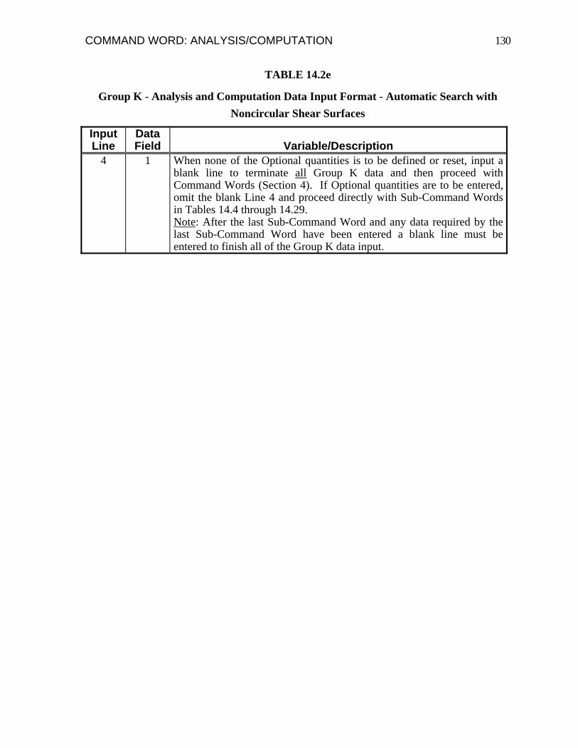
COMMAND WORD: ANALYSIS/COMPUTATION 130
TABLE 14.2e
Group K - Analysis and Computation Data Input Format - Automatic Search with Noncircular Shear Surfaces
Input Line
Data Field
Variable/Description
4 1 When none of the Optional quantities is to be defined or reset, input a blank line to terminate all Group K data and then proceed with Command Words (Section 4). If Optional quantities are to be entered, omit the blank Line 4 and proceed directly with Sub-Command Words in Tables 14.4 through 14.29. Note: After the last Sub-Command Word and any data required by the last Sub-Command Word have been entered a blank line must be entered to finish all of the Group K data input.

COMMAND WORD: ANALYSIS/COMPUTATION 131
TABLE 14.3
Summary of Sub-Command Words for Group K Data
Sub-Command "Word"
Description Table
1 Same as "SIN" - single-stage computations to be performed.
14.4
2 Same as "TWO" - two-stage computations to be performed.
14.4
3 Same as "THR" - three-stage computations to be performed.
14.4
ARC (Arc length)* Arc length to be used for subdivision of circles into slices.
14.5
BAS (Base length)* Maximum nominal base length to be used to subdivide noncircular shear surfaces into slices.
14.6
CHA (Change) Change the initial estimates for the factor of safety during the search.
14.7
CRA (Crack)* Crack depth. 14.8 CRI (Critical shear surface)
Critical shear surface is to be found by continuing the floating grid search after the first mode of search is completed.
14.9
FAC (Factor of safety)*
Initial trial factor of safety. 14.10
FOR (Force imbalance)*
Allowable force imbalance for convergence of solution for equilibrium equations.
14.11
INC (Increments for subdivision)*
Increments (nominal number of slices) to be used for subdividing noncircular shear surface into slices.
14.12
ITE (Iteration)* Maximum number of iterations allowed for iterative solution for the factor of safety.
14.13
LEF (Left) Left face of slope is to be analyzed. 14.14 LON (Long form) The long form of output is to be generated for the
automatic search. 14.15
MIN (Minimum weight)*
Minimum weight allowed for computations to be attempted.
14.16
MOM (Moment imbalance)*
Allowable moment imbalance for convergence of solution for equilibrium equations.
14.17
OPP (Opposite) "Opposite Sign Convention" option will be activated. 14.18 PAS (Passes)* The maximum number of "passes" allowed for a search
with noncircular shear surfaces. 14.19
PRO (Procedure of slices)*
Procedure of slices to be used to compute the factor of safety.
14.20
RES (Restrictions)* Restrictions on the limits (extent) of the shear surfaces for a search.
14.21
RIG (Right) Right face of slope is to be analyzed. 14.14 * Sub-Command Words requiring one or more additional lines of data to follow.

COMMAND WORD: ANALYSIS/COMPUTATION 132
TABLE 14.3 - Continued
Summary of Sub-Command Words for Group K Data
Sub-Command Word
Description Table
SAV (Save "n" most)*
Save the "n" most critical shear surfaces from the search. 14.22
SEI (Seismic coefficient)*
Seismic coefficient. 14.23
SHO (Short) The short-form of output is to be generated for the automatic search.
14.15
SID (Side force inclination)*
Initial trial value for the side force inclination for Spencer's procedure.
14.24
SIN (Single) Single-stage computations are to be performed. 14.4 SOR (Sort radii) Sort the radii which were varied to find a "critical" radius
in the order of increasing radius. Applicable to Type 2, "fixed" grid with circles only.
14.25
STO (Stop) Stop search with floating grid after the first "mode" has been completed.
14.9
SUB (Subtended angle)*
Subtended angle for subdividing circles into slices. 14.26
THR (Three) Three-stage computations are to be performed. 14.4 TRI (Trial)* The maximum number of trial, 9-point grids allowed for
each mode in the Type 1 search with "floating" grids - circles only.
14.27
TWO (Two) Two-stage computations are to be performed. 14.4 UNI (Unit weight of water)*
Unit weight of water (or other fluid) in the vertical "tension" crack.
14.28
UNS (Unsort) Do not sort the radii which were varied to find a critical radius - present them in the order they were examined. Applicable to Type 2, "fixed" grid with circles only.
14.25
WAT (Water)* Water depth in vertical tension crack. 14.29 * Sub-Command Words requiring one or more additional lines of data to follow.

COMMAND WORD: ANALYSIS/COMPUTATION 133
TABLE 14.4
Sub-Command: Computation Stages
Input Line
Data Field
Variable/Description
i 1 These Sub-Command Words are used to designate the number of stages for the computations as follows: • For conventional, single-stage computations specify “SIN” (or
"SINGLE-STAGE") or "1" - omit quotes ("). • For two-stage computations specify “TWO” (or “TWO-
STAGE”) or "2" - omit quotes ("). • For three-stage computations specify “THR” (or “THREE-
STAGE”) or "3" - omit quotes ("). Single stage computations are assumed as the default. Thus, the Sub-Command Word SIN is only used when multi-stage (2-stage or 3-stage) computations have been designated in the input data for previous set of computations and you are now returning to conventional, single-stage computations. Multi-stage (2-stage & 3-stage) computations are ordinarily only designated for rapid drawdown and, some forms of pseudo-static earthquake analyses. No additional lines of data with numerical values, etc., are needed immediately after these Sub-command Words.
TABLE 14.5
Sub-Command: Slice Arc Length (Circles Only)
Input Line
Data Field
Variable/Description
i 1 Sub-Command Word: "ARC" (or "ARC LENGTH") to designate that the circle is to be subdivided into slices using a prescribed maximum arc length for the base of slices as a criterion for subdivision; the next line of input designates the maximum arc length to be used. Circles are subdivided into slices using either a maximum arc length or maximum subtended angle (See Table 14.26); a maximum subtended angle of three degrees (3°) is the default criterion.
ii 1 Maximum subtended arc length between radii extending to each side of the base of a slice, Δ max (See Fig. 14.1).

COMMAND WORD: ANALYSIS/COMPUTATION 134
TABLE 14.6
Sub-Command: Nominal Slice Base Length (Noncircular Only)
Input Line
Data Field
Variable/Description
i 1 Sub-Command Word: "BAS" (or "BASE LENGTH") to designate that the noncircular shear surface is to be subdivided into slices using a maximum slice base length as a criterion for subdivision; the next line of input designates the maximum length to be used. Noncircular shear surfaces are subdivided into slices using either the maximum slice base length or the nominal number of slices as a criterion (See also Table 14.12); the latter criterion with a nominal number of thirty (30) slices is used as the default.
ii 1 Maximum length allowed for the base of slices after subdivision, Δ max. Slice boundaries are always located at points where coordinates were specified for the noncircular shear surfaces as well as at other points where coordinates are specified, etc.; the maximum length specified on this line of input is a maximum only, many slices may have bases whose length is smaller.
TABLE 14.7
Sub-Command: Change Initial Estimates for Factor of Safety During Automatic Searches
Input Line
Data Field
Variable/Description
i 1 Sub-Command Word: "CHA" (or "CHANGE") to change the initial estimates for the factor of safety (and side force inclination in the case of Spencer's procedure) during the search; the values associated with the most critical shear surface found to that point in the search are used.

COMMAND WORD: ANALYSIS/COMPUTATION 135
TABLE 14.8
Sub-Command: Vertical “Tension” Crack
Input Line
Data Field
Variable/Description
i 1 Sub-Command Word: "CRA" (or "CRACK") to designate that the supplemental data on the next lines of input are for the crack depth. If either the crack depth is constant or the elevation of the bottom of the crack is constant proceed with Line ii; Otherwise proceed with Line iiB.
iiA 1 A numerical value designating either (1) the crack depth or (2) the elevation of the bottom of the crack, depending on the character in the next field.
iiA 2 A character or a character string beginning with either: E - if the value in Field 1 is the elevation of the bottom of the crack. D - if the value in Field 1 is the depth of the crack.
If crack depth is constant or the elevation of the bottom of the crack is constant, you are done; proceed with additional Sub-Command Words in Tables 14.4 through 14.29.
iiB 1 A character or a character string beginning with one of the following characters to designate if the data which are to follow are for the elevation of the bottom of the crack or the crack depth profile: E - if the value in Field 1 is the elevation of the bottom of the crack. D - if the value in Field 1 is the depth of the crack.
iiiB 1 X coordinate of point on a line defining either the depth of the crack or the bottom of the crack, depending on what was designated on Line iiB.
iiiB 2 Either the depth of the crack or the elevation of the bottom of the crack at the x coordinate designated in Field 1 of Line iiiB.
Repeat Line(s) iiiB to define additional points on the crack profile in a left-to-right sequence. More than one pair of values may be entered on a given line of input data if desired; however, each line must contain complete pairs (2 values) for each point. Input a blank line to terminate data for the variable crack profile. Note: UTEXAS4 distinguishes between constant vs. variable crack depths and elevations based on what is entered on the first line (iiA, iiB) after the Sub-Command Word, "CRACK": If the line (iiA, iiB) contains a numerical value a constant value is assumed for the crack depth or elevation; if the line of input begins with a non-numerical value (E or D), a variable crack depth or crack elevation is assumed.

COMMAND WORD: ANALYSIS/COMPUTATION 136
TABLE 14.9
Sub-Command: Search Termination (Type 1, “Floating” Grid Search Only)
Input Line
Data Field
Variable/Description
i 1 Sub-Command Word: "STO" (or "STOP") to designate that the “floating” grid search is to be stopped after the first Step/Mode is completed. In this case the first step of the search will be conducted to find the critical circle according to the initial “mode” and the search will then be stopped. This may be useful if only a critical circle tangent to a given line (depth) or through a prescribed point is of interest. It is also useful if you want to manually conduct searches for various modes, e. g. for various tangent lines.
/OR/ Sub-Command Word: "CRI" (or "CRITICAL") to designate that the “floating grid” search is to be continued in the normal manner, alternating search “modes”, until a most critical circle is found. This is the normal, default condition. This sub-command word (CRI) is only needed when the option is to be reset for a new search after having been set to STOP as described above.
TABLE 14.10
Sub-Command: Initial Trial Factor of Safety
Input Line
Data Field
Variable/Description
i 1 Sub-Command Word: "FAC" (or "FACTOR OF SAFETY") to designate that an initial trial value for the factor of safety is to be entered. For each trial shear surface an iterative (trial and error) solution is used to compute the factor of safety. A default value is assumed and may be overridden by use of this Sub-Command Word.
ii 1 Initial trial value for factor of safety, F0.

COMMAND WORD: ANALYSIS/COMPUTATION 137
TABLE 14.11
Sub-Command: Force Imbalance Allowed for Convergence
Input Line
Data Field
Variable/Description
i 1 Sub-Command Word: "FOR" (or "FORCE IMBALANCE") to designate that the maximum allowable force imbalance is to be entered. In Spencer’s and the Force Equilibrium procedures an iterative (trial and error) solution is used to compute the factor of safety. Iterations are continued until force imbalance is less than a maximum acceptable value. A default value is assumed for the maximum acceptable force imbalance and may be overridden by use of this Sub-Command Word. The default value is defined in the UTEXAS4 Application Settings (See Section 2).
ii 1 Value designating the maximum allowable force imbalance. Depending on what is entered in the second field of this line of input the value should represent one of the following: (1) The actual maximum force imbalance allowed – specified as the
value of force in appropriate force units. (Leave Field 2 blank). (2) The maximum allowable force imbalance expressed as a
decimal fraction of the weight. (Field 2 must contain a character or characters as described below.)
Must be a positive number greater than zero. Zero force imbalance can usually not be attained due to numerical round-off errors.
ii 2 Leave this field blank if the actual value of force was entered in Field 1. If the value entered in Field 1 represents the force imbalance as a decimal fraction of the total known forces, then you must enter a single character “D” or a character string beginning with character “D’ to signify that a decimal fraction is being entered.

COMMAND WORD: ANALYSIS/COMPUTATION 138
TABLE 14.12
Sub-Command: Nominal Slice Increments (Noncircular Only)
Input Line
Data Field
Variable/Description
i 1 Sub-Command Word: "INC" (or "INCREMENTS") to designate that the noncircular shear surface is to be subdivided into slices using a nominal number of increments (slices) as a criterion for subdivision; the next line of input designates the nominal number of increments to be used. Noncircular shear surfaces are subdivided into slices using either the nominal number of slices or a maximum slice base length as a criterion (See also Table 14.6); a nominal number of 30 slices is used as the default.
ii 1 Nominal number of increments (slices) into which the shear surface is to be subdivided, nnominal. Slices are subdivided by first taking the chord length between the two ends of the noncircular shear surface and dividing it by the nominal number of increments; the resulting length is then used as the maximum allowable base length for subdivision into slices (See Table 14.6)
TABLE 14.13
Sub-Command: Maximum Number of Iterations
Input Line
Data Field
Variable/Description
i 1 Sub-Command Word: "ITE" (or "ITERATIONS") to designate that the maximum number of iterations is to be entered. An iterative (trial and error) solution is used to compute the factor of safety and, in the case of Spencer’s procedure, the side force inclination. Iterations are continued until force and/or moment imbalances are less than a maximum acceptable value OR until a maximum number of iterations is exceeded. A default value is assumed for the maximum number of iterations and may be overridden by use of this Sub-Command Word.
ii 1 Maximum number of iterations.

COMMAND WORD: ANALYSIS/COMPUTATION 139
TABLE 14.14
Sub-Command: Slope Face Selection (Circles Only)
Input Line
Data Field
Variable/Description
i 1 Sub-Command Word: "LEF" (or "LEFT") to designate that only the left face of the slope will be analyzed; trial shear surfaces for the right face will be automatically rejected.
/OR/ Sub-Command Word: "RIG" (or "RIGHT") to designate that only the right face of the slope will be analyzed; trial shear surfaces for the left face will be automatically rejected.
TABLE 14.15
Sub-Command: Output Format for Search
Input Line
Data Field
Variable/Description
i 1 These Sub-Command Words are used to designate the form of output (short vs. long) required from the automatic search. See the description in Section 15 of the output tables created by UTEXAS4. Sub-Command Word: "LON" (or "LONG") to designate the long-form of search output is requested.
/OR/ Sub-Command Word: "SHO" (or "SHORT") to designate that the short-form of search output is requested.
TABLE 14.16
Sub-Command: Minimum Weight for Computations
Input Line
Data Field
Variable/Description
i 1 Sub-Command Word: "MIN" (or "MINIMUM") to designate that the minimum weight of soil allowed for computations to be performed will be entered on the next line of input. UTEXAS4 rejects all trial shear surface where the total weight is less than a designated minimum value.
ii 1 Minimum weight allowed for computations. If zero is entered and the allowable force and moment imbalances are defined in terms of actual values (rather than as decimal fractions), the minimum weight will be taken as 0.001 times the designated force imbalance.

COMMAND WORD: ANALYSIS/COMPUTATION 140
TABLE 14.17
Sub-Command: Moment Imbalance Allowed for Convergence
Input Line
Data Field
Variable/Description
i 1 Sub-Command Word: "MOM" (or "MOMENT IMBALANCE") to designate that the maximum allowable moment imbalance is to be entered. In Spencer’s and the Simplified Bishop procedures an iterative (trial and error) solution is used to compute the factor of safety. Iterations are continued until the moment imbalance is less than a maximum acceptable value. A default value is assumed for the maximum acceptable moment imbalance and may be overridden by use of this Sub-Command Word. See also Tables 14.11 and 14.13 for Force Imbalance and Maximum Iterations.
ii 1 Value designating the maximum allowable moment imbalance; all moments are taken and expressed as moments about the origin (x = 0, y = 0) of the coordinate system. Depending on what is entered in the second field of this line of input the value should represent one of the following: (1) The actual maximum moment imbalance allowed – specified as
a value of moment in appropriate units, e. g. pound-feet, Newton-meters, etc.
(2) The maximum allowable moment imbalance expressed as a decimal fraction of the moment produced by the soil weight and computed about the origin of the coordinate system. (Field 2 must contain a character or characters as described below.)
Must be a positive number greater than zero. Exactly zero moment imbalance can usually not be attained due to numerical round-off errors.
ii 2 Leave blank if the actual value of moment was entered in Field 1. If the value entered in Field 1 represents the moment imbalance as a decimal fraction of the moment due to the weight of soil above the shear surface, then you must enter a single character “D” or a character string beginning with character “D’ to signify that a decimal fraction is being entered.

COMMAND WORD: ANALYSIS/COMPUTATION 141
TABLE 14.18
Sub-Command: Opposite Sign Convention
Input Line
Data Field
Variable/Description
i 1 Sub-Command Word: “OPP” (or “OPPOSITE) to activate the “opposite sign convention” option. This Sub-Command Word is used when the shear forces along the shear surface act in the opposite direction from what they normally would for the direction the slope faces. For example, if the slope faces to the left, but sliding will occur from left to right, the opposite sign convention option must be used. This may be necessary when, for example, distributed loads or line loads force the failure to be in an “upslope” direction.
TABLE 14.19
Sub-Command: Maximum Number of Passes (Searches with Noncircular Shear Surfaces)
Input Line
Data Field
Variable/Description
i 1 Sub-Command Word: “PAS” (or “PASSES) to designate that the maximum number of passes for shifting the noncircular shear surface during an automatic search will follow on the next line of data.
ii 1 Maximum number of “passes” that will be attempted for a search with noncircular shear surfaces.

COMMAND WORD: ANALYSIS/COMPUTATION 142
TABLE 14.20
Sub-Command: Procedure of Analysis
Input Line
Data Field
Variable/Description
i 1 Sub-Command Word: "PRO" (or "PROCEDURE") to designate that the procedure of slices used to compute the factor of safety will be designated on the next line of input. UTEXAS4 assumes as a default that Spencer's procedure will be used. This Sub-Command Word is used to select a different procedure.
ii 1 A character or character string beginning with one of the following characters to designate the procedure of analysis to be used: S = Spencer’s procedure will be used. (Spencer's procedure is the
default procedure. Thus, this option is only necessary when another procedure was used and you are returning to use Spencer's procedure).
B = Bishop’s simplified procedure will be used. C = Corps of Engineers’ Modified Swedish force equilibrium
procedure will be used. (Also can be used to designate Simplified Janbu procedure - See Line iii below).
L = Lowe and Karafiath’s force equilibrium procedure will be used.If the Corps of Engineers’ Modified Swedish procedure is designated, enter Line iii; otherwise skip Line iii.
iii 1 Side force inclination (in degrees) - measured from the horizontal plane. The specified value for the side force inclination should be positive for side forces inclined in the same direction as the slope and negative for side force inclinations that are in the opposite direction. For the Corps of Engineers’ procedure specify the appropriate value in accord with Corps of Engineers’ guidelines; for the Simplified Janbu procedure specify zero, i. e. horizontal side forces.

COMMAND WORD: ANALYSIS/COMPUTATION 143
TABLE 14.21
Sub-Command: Search Restrictions
Input Line
Data Field
Variable/Description
i 1 Sub-Command Word: "RES" (or "RESTRICTIONS") to designate that data which follow are for restrictions on the lateral extent of shear surfaces that will be imposed during the automatic search for either circular or noncircular shear surfaces. Several sets of restrictions may be placed on the limits of the shear surface for a given search.
ii 1, 2 A pair of characters or pair of character strings beginning with the following pair of letters to designate the form of the restrictions that will follow on Line iii. A E (or "ABSOLUTE" "ENTIRE"): The restrictions will be specified in terms of absolute x coordinates and the entire shear surface must lie within the specified restriction limits. A S (or "ABSOLUTE" "SOME"): The restrictions will be specified in terms of absolute x coordinates and only some of the shear surface must lie within the specified restriction limits. R E (or "RELATIVE" "ENTIRE"): The restrictions are relative to the center of the circle and the entire shear surface must lie within the specified restriction limits - applicable to circles only. R S (or "RELATIVE" "SOME"): The restrictions are relative to the center of the circle and only some of the shear surface must lie within the specified restriction limits - applicable to circles only.
iii 1 Depending on whether the restrictions are absolute (A) or relative (R): If absolute, the minimum x coordinate defining the left-most boundary of the restriction zone. If relative, the horizontal distance from the center of the circle to the left-most boundary of the restriction zone. Negative values for points to the left of the center of the circle; positive values for points to the right of the center.
iii 2 Depending on whether the restrictions are absolute (A) or relative (R): If absolute, the maximum x coordinate defining the right-most boundary of the restriction zone. If relative, the horizontal distance from the center of the circle to the right-most boundary of the restriction zone. Negative values for points to the left of the center of the circle; positive values for points to the right of the center.
Repeat Lines ii and iii for additional restrictions on the search. Shear surfaces must satisfy all restrictions specified in order to be used; when several restrictions are designated, failure to meet any one will cause the shear surface to be rejected.

COMMAND WORD: ANALYSIS/COMPUTATION 144
TABLE 14.22
Sub-Command: Number of Shear Surfaces to be Saved (Searches Only)
Input Line
Data Field
Variable/Description
i 1 Sub-Command Word: "SAV" (or "SAVE") to designate that the number of “most critical” shear surfaces to be saved will follow on the next line of input. Ordinarily only the most critical shear surface is saved and available for display later. This Sub-Command Word allows you to designate a number of the most critical shear surfaces to be saved. The factors of safety for these shear surfaces will then be summarized and the shear surfaces will be available for display later using TexGraf4.
ii 1 Number of the most critical (lowest factor of safety) shear surfaces to be saved.
TABLE 14.23
Sub-Command: Seismic Coefficient
Input Line
Data Field
Variable/Description
i 1 Sub-Command Word: “SEI” (or “SEISMIC) to designate that a seismic coefficient will be entered on the next line of input.
ii 1 Value for the seismic coefficient. Positive values for seismic loads acting away from the slope, negative values for seismic forces acting into the slope. A default value of zero (no seismic forces) is assumed if none are specified.
ii 2 The seismic forces are normally applied at the center of gravity of the slice. This data field can contain an optional 3-character string or longer character-string beginning with the following three characters to designate otherwise as follows: MID (or “MID-HEIGHT”) - seismic forces are applied at mid-height of the slice. BOT (or “BOTTOM”) - seismic forces are applied to the bottom of the slice - at the shear surface. If neither of the above strings is specified, the seismic forces will be applied through the center of gravity of the slice. (Note: The center of gravity and mid-height may differ when the unit weights vary over the height of the slice.)

COMMAND WORD: ANALYSIS/COMPUTATION 145
TABLE 14.24
Sub-Command: Initial Trial Side Force Inclination
Input Line
Data Field
Variable/Description
i 1 Sub-Command Word: "SID" (or "SIDE FORCE INCLINATION") to designate that an initial trial value for the side force inclination is to be entered. In Spencer’s procedure an iterative (trial and error) solution is used to compute the side force inclination. A default value is assumed and may be overridden by use of this Sub-Command Word. Note: This variable is only used in Spencer’s procedure; it is ignored in all other procedures.
ii 1 Initial trial value for side force inclination (in degrees).
TABLE 14.25
Sub-Command: Sorted/Unsorted Radii (Type 2 "Fixed Grid" Search Only)
Input Line
Data Field
Variable/Description
i 1 These Sub-Command Words (“SOR” and “UNS”) apply to a Type 2 search with a fixed grid and control the order that the results for individual circles are presented. Two series of output involve sorting: (1) For a given grid (center) point the various radii attempted may
be sorted in the order of increasing radius or left in the order that the various trial radii were attempted.
(2) For all of the grid points the final summary of minimum factors of safety for each grid point may be sorted in the order of increasing factor of safety - lowest factor of safety first – or left in the order that the individual grid points were processed.
Sub-Command Word: “UNS” (or “UNSORTED”) designates that the output will not be sorted: Circles (radii) for individual grid points will be presented in the order they were calculated and critical circles for each grid point will be presented in the order grid points were examined.
/OR/ Sub-Command Word: “SOR” (or “SORT”) to designate that the output will be sorted: Circles (radii) for individual grid points will be sorted in the order of increasing radius and critical circles for all grid points will be output in the order of increasing factor of safety; lowest factor of safety first. These Sub-Command Word are only applicable for a Type 2 search with a fixed grid.

COMMAND WORD: ANALYSIS/COMPUTATION 146
TABLE 14.26
Sub-Command: Slice Subtended Angle (Circles Only)
Input Line
Data Field
Variable/Description
i 1 Sub-Command Word: "SUB" (or "SUBTENDED ANGLE") to designate that the circle is to be subdivided into slices using the maximum subtended angle of the base of slices as a criterion for subdivision; the following line of input designates the maximum subtended angle to be used. Circles are subdivided into slices using either a maximum subtended angle or a maximum arc length (See Table 14.5); a maximum subtended angle of three degrees (3°) is the default criterion.
ii 1 Maximum subtended angle formed by radii extending to each side of the base of a slice, Δθmax.
TABLE 14.27
Sub-Command: Maximum Number of Trials (Type 1, “Floating” Grid Search Only)
Input Line
Data Field
Variable/Description
i 1 Sub-Command Word: "TRI" (or "TRIAL") to designate that the maximum number of trials for an automatic search using a floating grid and circular shear surfaces will be entered on the next line of data. The default number of grids is 50.
ii 1 Maximum number of trial, 9-point grids that will be used for a given mode of search before abandoning the solution.
TABLE 14.28
Sub-Command: Unit Weight for Water in “Tension” Crack
Input Line
Data Field
Variable/Description
i 1 Sub-Command Word: "UNI" (or "UNIT WEIGHT") to designate that a unit weight is to be entered for the water (or other fluid) in the tension crack. Default values for the unit weight of water are set in the UTEXAS4 Application Settings (See Section 2) and depend on the current set of units.
ii 1 Value for the unit weight of fluid in the crack.

COMMAND WORD: ANALYSIS/COMPUTATION 147
TABLE 14.29
Sub-Command: Tension “Crack” Water
Input Line
Data Field
Variable/Description
i 1 Sub-Command Word: "WAT" (or "WATER") to designate that the supplemental data which immediately follow are for the water in a “tension” crack. (Separate data for the crack itself must be input as indicated in Table 14.8.) The water levels may either be defined by a single value of water elevation or depth (Line iiA) or by a series of points defining the water depth or elevations (Lines iiB & iiiB). If either the water depth is constant or the elevation of the water surface is constant, use the Line iiA format; otherwise use the format for Lines iiB and iiiB.
iiA 1 A numerical value designating either (1) the water depth in the crack or (2) the elevation of the water surface in the crack, depending on the character in the next field.
iiA 2 A character or a character string beginning with either: E: if the value in Field 1 is the elevation of the water surface for the
crack. D: if the value in Field 1 is the depth of the water in the crack.
If the depth is constant or the elevation of the water surface is constant, you are done; proceed with additional Sub-Command Words.
iiB 1 A character or a character string beginning with one of the following characters (E or D) to designate if the data which will follow on Lines iiiB are for the elevation of the water in the crack or the water depth profile: E: If the values on Lines iiiB define the elevation of the water
surface in the crack. D: If the values on Lines iiiB define the depth of water in the crack.
iiiB 1 X coordinate of point on a line defining either the depth of the water or the elevation of the water surface in the crack, depending on what was designated on Line iiB.
iiiB 2 Either the depth of the water or the elevation of the water surface in the crack at the x coordinate designated in Field 1 of this line of input.
Repeat Line(s) iiiB to define additional points on the crack water profile in a left-to-right sequence. More than one pair of values may be entered on a given line of input if desired; however, each line must contain complete pairs (2 values) for each point. Input a blank line to terminate data for the variable crack water profile.

COMMAND WORD: ANALYSIS/COMPUTATION 148
θ
Δ
Figure 14.1 - Illustration of Subtended Angle and Arc Length Used as Criteria for Subdivision of Circular Shear Surfaces into Slices.

COMMAND WORD: ANALYSIS/COMPUTATION 149
dcrack
"Tension" crackNeglected
Zone
Figure 14.2 - Vertical "Tension" Crack Showing Depth of Crack and Zone of Soil Above Shear Surface That is Neglected in Stability Computations.

COMMAND WORD: ANALYSIS/COMPUTATION 150
Figure 14.3 - Position of Vertical Tension Crack for Three Different Circles.

COMMAND WORD: ANALYSIS/COMPUTATION 151
L
R
τ
(a) Left-Facing Slope (yR > yL).
R
L
τ
(b) Right-Facing Slope (yR < yL).
Figure 14.4 - Slope Face Criteria and Direction of Resisting Shear Stress on Slide Mass for Left-Facing and Right-Facing Slopes

COMMAND WORD: ANALYSIS/COMPUTATION 152
τ
Figure 14.5 - Direction of Sliding and Direction of Resisting Shear Stress on Slide Mass Assumed for Horizontal Ground.

COMMAND WORD: ANALYSIS/COMPUTATION 153
Figure 14.6 - Circle Intersecting both Left and Right Faces of a Slope.

COMMAND WORD: ANALYSIS/COMPUTATION 154
τ
(a) Direction of Resisting Shear Stress on Slide Mass Assumed for "Normal" Conditions.
τ
(b) Direction of Resisting Shear Stress on Slide Mass for "Optional Sign Convention" Condition.
Figure 14. 7 - Direction of Resisting Shear Stress on Slide Mass for "Normal" and Optional ("Opposite Sign Convention") Conditions.

COMMAND WORD: ANALYSIS/COMPUTATION 155
τ Figure 14.8 - Direction of Resisting Shear Stress on Soil Mass for Horizontal Ground When the "Opposite Sign Convention" Option is Activated.

COMMAND WORD: ANALYSIS/COMPUTATION 156
1st Step2nd Step
1st Step local m inimum
1st Step local m inimum
1st Step local m inimum
Factor of Safety
Rad
ius
Rm in
Rmax
Rmin.
Rmax.
Figure 14.9 - Illustration of Variation in Factor of Safety with Radius After Initial Incrementing of Radii.

COMMAND WORD: ANALYSIS/COMPUTATION 157
New minimum #1
New minimum #2
Rmax
Rmin
Rad
ius
Rad
ius
Rmax
Rmin
InitialMinimum
(a) First Step (b) After second step
Factor of Safety Factor of Safety
Figure 14.10 - Refinement of Trial Radii for Multiple Local Minima.
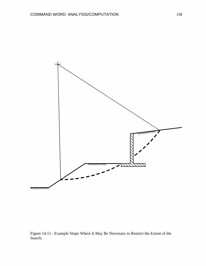
COMMAND WORD: ANALYSIS/COMPUTATION 158
Figure 14.11 - Example Slope Where It May Be Necessary to Restrict the Extent of the Search.

COMMAND WORD: ANALYSIS/COMPUTATION 159
xleft xright xleft xright
Accepted Rejected
(a) Entire Shear Surface Required to be within Limits
xleft xright xleft xright
Accepted Rejected
(b) Some of Shear Surface Required to be within Limits
Figure 14.12 - Illustration of Search Restrictions Specified in Terms of Absolute Limits.

COMMAND WORD: ANALYSIS/COMPUTATION 160
Δxleft Δxright
Accepted Rejected
Δxleft Δxright
(a) Entire Shear Surface Required to be within Limits
Accepted Rejected
Δxleft Δxright Δxleft Δxright
(b) Some of Shear Surface Required to be within Limits
Figure 14.13 - Illustration of Search Restrictions Specified in Terms of Relative Limits.

COMMAND WORD: ANALYSIS/COMPUTATION 161
Zi
Zi+1
yt,i yt,i+1
N
(a) Spencer's Procedure.
Zi
Zi+1
NN
(b) Simplified Bishop Procedure (c) Force Equilibrium Only Procedures (Corps of Engineers' Modified Swedish; Lowe and Karafiath; "Simplified Janbu").
Figure 14.14 - Additional "Unknowns" (Besides Factor of Safety and Side Force Inclination) Calculated in Various Procedures of Slices Implemented in UTEXAS4.

COMMAND WORD: ANALYSIS/COMPUTATION 162
+-
(a) Left-Facing Slope
(b) Right-Facing Slope Figure 14.15 - Sign Convention for Data Input of Side Force Inclinations.

COMMAND WORD: ANALYSIS/COMPUTATION 163
-+
(a) Left-Facing Slope
(b) Right-Facing Slope
Figure 14.16 - Sign Convention for Side Force Inclinations Used for Computations and Output.

COMMAND WORD: ANALYSIS/COMPUTATION 164
- 10°
+ 80°
(a) Left-Facing Slope
+ 10°
- 80°
(b) Right-Facing Slope Figure 14.17 - Limits on Side Force Inclinations for Left-Facing and Right-Facing Slopes.

OUTPUT TABLES
165
Section 15 - DESCRIPTION AND EXPLANATION OF PRINTED OUTPUT TABLES
Introduction
Sixty (60) different types of output tables are printed by UTEXAS4. The forms of these tables and the information which they contain are described in this section. Each type of table is identified by a table number for reference and identification. The table number is printed on the computer output at the start of each table and corresponds to the type of information which the table contains. Tables are printed in the order in which the information contained in the tables are either input to, or generated by, the computer program. Accordingly, tables will not necessarily be printed in the order of ascending or descending table numbers. Some tables may not be printed at all, and other tables may be printed several times, depending on the type of data which are input and the program options which are used.
The first output table (Output Table 1) contains general information pertaining to the computer program and is printed only once at the start of program execution. The remaining Output Tables start on a new page of output with a four- or five- line header containing the version and revision dates for UTEXAS4, the name and organization of the licensee, the time and date that computations were initiated, and the name of the input data file. The next lines of output contain the heading which you entered as Group A data. A table number in accordance with the numbering system described in this section is then printed. For most output tables a descriptive banner is printed immediately following the table number to describe what the table contains. The format of this banner and some of the other information in the output tables depend in part on whether the data are input data are part of the solution.
Output Tables for Input Data
The first twenty-four tables following Output Table 1 (Output Table Nos. 2 through 25) contain data which are used to define the problem. All of these twenty-four tables contain data which you input. Each of these twenty-four tables is printed separately any time the specific data contained in the table is changed by new input data. If a specific set of data is not changed, the corresponding table will not be printed.
The banner containing the description of the table that follows the table number contains a border that depends on whether the data are for conventional (single-stage)

OUTPUT TABLES 166
analyses or multi-stage analyses. For conventional, single-stage analyses or the first-stage of multi-stage analyses, the banner is enclosed by a rectangle of asterisks (*** etc.). For example the banner for Output Table 4, which contains the material properties would appear as:
********************************************************************** * NEW MATERIAL PROPERTY DATA - CONVENTIONAL/FIRST-STAGE COMPUTATIONS * **********************************************************************
In the case of information for the second- and third- stage of multi-stage computations a similar banner is printed, except that the rectangle framing the banner is printed as two's (222 etc.). For example, the banner for Output Table 5 which contains material properties for the second- and third- stages of multi-stage computations would be printed as:
2222222222222222222222222222222222222222222222222222222222 2 NEW MATERIAL PROPERTY DATA - SECOND-STAGE COMPUTATIONS 2 2222222222222222222222222222222222222222222222222222222222
Output Tables for Computed Results
The remaining thirty-five output tables (Output Tables 26 through 60) contain information which is generated by UTEXAS4 during computations. These thirty-five tables contain intermediate information, as well as the final solution. The banner for tables which contain information covering all stages of the computations are printed with borders of asterisks (*** etc.). Similarly if conventional, single stage computations are performed the banners for the descriptive heading on tables are also all printed with asterisks. For multi-stage computations, the banners are printed with strings of numbers (111, 222, 333) to indicate the stage when the information in the table corresponds to a specific stage of the computations. Banners with information for the first stage have borders consisting of the numeral "1"; banners for the second stage have banners with the numeral "2"; and banners for the final stage are printed with a border of 3's.
For automatic searches there are two forms of output tables that may be generated: "Short-Form" and "Long-Form." The Long-Form of output is the default setting and is strongly encouraged, at least until results have been inspected for correctness. The Short-Form of output tables are abbreviated and contain much less information that the Long-Form. The Short-Form of output is activated with the Sub-Command word, "SHORT", which is entered with the Analysis/Computation data as described in Section 14.

OUTPUT TABLES 167
Output Table Contents
Output Table 1 - Program Header
Output Table 1 contains the UTEXAS4 header message: The program name (UTEXAS4), version number, copyright notice, disclaimer and warning message. Output Table 1 is printed only once at the start of execution.
Output Table 2 – Units Data
Output Table 2 contains the information pertaining to the type of units and corresponding default values that will be used. This table is printed whenever the input data designates a set of units (via the unit Command Words ENG, SIU or OTH as described in Section 4). The table is not printed for the default units.
Output Table 3 - Input Data for Profile Lines
This table contains the input data for the Profile Lines (Group B data). The table is printed every time new Profile Line data are input to the program and only when new data are input. Any data which have been previously input and retained when the new data are input are not printed again. Instead, a message is printed that previous data are retained and you should refer to earlier output.
Output Table 4 - Input Data for Material Properties (Stage 1)
Output Table 4 contains the input data for material properties (Group C data) for conventional computations or the first-stage of multi-stage computations; Output Table 4 contains the material properties for the second and third stages of multi-stage computations. The table is printed each time new material property data are input and only when new data are input. Any data for materials which are retained from previous input are not printed again. Instead, a message is printed to designate the number of materials for which previous data are retained; you should refer to earlier printed output tables for the retained data.
Output Table 5 - Input Data for Material Properties (Stage 2)
Output Table 5 contains the data for the material properties for the second and third stages of multi-stage computations. The form of the table and rules governing when the table is printed are identical to those for Output Table 4.
Output Table 6 - Input Data for Piezometric Lines (Stage 1)
Output Table 6 contains the input data for the piezometric lines (Group D data) for conventional computations or the first-stage of multi-stage computations. The table is printed every time you input new piezometric line data and only when new data are input.

OUTPUT TABLES 168
Any data which have been previously input and retained when the new data are input are not printed again. Instead, a message is printed that previous data are retained and you should refer to earlier output.
Output Table 7 - Input Data for Piezometric Lines (Stage 2)
Output Table 7 contains the data for the piezometric lines for the second and third stages of multi-stage computations. The form of this table and rules governing when the table is printed are identical to those for Output Table 6.
Output Table 8 - Input Data for Pore Water Pressure and Shear Strength Interpolation (Stage 1)
Output Table 8 contains the input data used for interpolation of pore water pressure, ru values and undrained shear strengths (Group E data) for conventional computations or the first-stage of multi-stage computations. The tables are created whenever these data are input. If only some of the data are new and other data input previously are retained, only the new data are printed. A message will be printed indicating that previous data were not printed again. You should refer to earlier output tables for the data which are retained.
Output Table 9 - Input Data for Pore Water Pressure and Shear Strength Interpolation (Stage 2)
Output Table 9 contains the input data used for interpolation of pore water pressure, ru values and undrained shear strengths (Group E data) for the second and third stages of multi-stage computations. The form of the table and rules governing when the table is printed are identical to those for Output Table 8.
Output Table 10 - Input Data for Slope Geometry
This table contains the coordinates defining the slope geometry (Group F data) when the coordinates are specifically defined as input data (See also Output Table 26). The table is printed whenever the coordinates are defined or redefined by input data. This table is printed only when the slope coordinates are defined specifically by Group F input data (See Output Table 26 for the case where slope coordinates are generated by the program).
Output Table 11 - Input Data for Distributed Loads (Stage 1)
This table contains the input data for the distributed loads (stresses) acting on the surface of the slope (Group G data) for conventional computations or the first-stage of multi-stage computations. The table is printed only when these data are defined or redefined by new input data.

OUTPUT TABLES 169
Output Table 12 - Input Data for Distributed Loads (Stage 2)
Output Table 12 contains the distributed load data for the second and third stages of multi-stage computations. The form of the table and rules governing when the table is printed are identical to those for Output Table 12.
Output Table 13 - Input Data for Line Loads (Stage 1)
Output Table 13 contains the input data for internal and external line loads (Group H data) for conventional computations or the first-stage of multi-stage computations. The table is created only when these data are defined or redefined by new input data.
Table14 - Input Data for Line Loads (Stage 2)
Output Table 14 contains the line load data for the second and third stages of multi-stage computations. The table is printed only when these data are defined or redefined by new input data.
Output Table 15 - Input Data for Reinforcement
This table contains the input data used to describe the internal soil reinforcement (Group J data). The table is printed every time new soil reinforcement data are input and only when new data are input. Any data which have been previously input and retained when new data are input are not printed again. Instead, a message is printed that previous data are retained and you should refer to earlier output.
Output Table 16 - Input Data for Analysis/Computations
This table contains the information for the analysis and computations which is input by means of Group K data. The table is printed only when new Group K data are input. In addition to containing the values input as data, the table contains values of parameters which either were set as default values by UTEXAS4 or were defined by previous input data.
Output Table 17 – Modified Input Data for Profile Lines
Output Table 17 contains revised coordinates for the Profile Lines when ether duplicate points have been detected or points were in the reverse order (right-to-left). UTEXAS4 automatically discards duplicate coordinate points and if the points are entered in a right-to-left sequence, UTEXAS4 attempts to reverse the order of the points. When these changes are made the Profile Lines are reprinted in Output Table 17. The form of Output Table 17 is identical to Output Table 3.
The elimination and/or rearranging of points on the Profile Lines is only done once all data have been read and computations are about to be attempted. Accordingly, this table will be printed after all the tables of input data have been printed.

OUTPUT TABLES 170
Output Table 18 – Modified Input Data for Piezometric Lines (Stage 1)
Output Table 18 contains revised coordinates for the piezometric lines for conventional computations or the first-stage of multi-stage computations when ether duplicate points have been detected or the points were in the reverse order (right-to-left). UTEXAS4 automatically discards duplicate coordinate points and if the points are entered in a right-to-left sequence, UTEXAS4 attempts to reverse the order of the points. When these changes are made the Piezometric Lines are reprinted in Output Table 18. The form of Output Table 18 is identical to Output Table 6.
The elimination and/or rearranging of points on the piezometric lines is only done once all data have been read and computations are about to be attempted. Accordingly, this table is printed after all the tables of input data have been printed.
Output Table 19 – Modified Input Data for Piezometric Lines (Stage 2)
This table is identical to Output Table 18 except it contains data for the second and third stages of multi-stage computations.
Output Table 20 – Modified Input Data for Pore Water Pressure and Shear Strength Interpolation (Stage 1)
Output Table 20 contains revised interpolation data for conventional computations or the first-stage of multi-stage computations when duplicate points have been detected. UTEXAS4 automatically discards duplicate interpolation points. When points are discarded the interpolation data points are reprinted in Output Table 20. The form of Output Table 20 is identical to Output Table 8.
The elimination of duplicate interpolation data points is only done once all input data for a particular set of computations have been read and computations are about to be attempted. Thus, this table is printed after all the tables of input data have been printed.
Output Table 21 – Modified Input Data for Pore Water Pressure and Shear Strength Interpolation (Stage 2)
This table is identical to Output Table 21 except it contains data for the second and third stages of multi-stage computations.
Output Table 22 – Modified Input Data for Slope Geometry
Output Table 22 contains revised coordinates for the slope geometry when ether duplicate points have been detected or the points were in the reverse order (right-to-left). UTEXAS4 automatically discards duplicate coordinate points and if the points are entered in

OUTPUT TABLES 171
a right-to-left sequence, UTEXAS4 attempts to reverse the order of the points. When these changes are made the Slope Geometry points are reprinted in Output Table 22. The form of Output Table 22 is identical to Output Table 10.
The elimination and/or rearranging of points for the slope geometry is only done once all data have been read and computations are about to be attempted. Accordingly, this table is printed after all the tables of input data have been printed.
Output Table 23 – Modified Input Data for Distributed Loads (Stage 1)
Output Table 23 contains revised data for the distributed loads for conventional computations or the first-stage of multi-stage computations when the points have been detected to be in reverse order (right-to-left rather than left-to-right). UTEXAS4 automatically rearranges the points in a left-to-right sequence if the points are entered in a right-to-left sequence. When the points are rearranged the Distributed Laods are reprinted in Output Table 23. The form of Output Table 23 is identical to Output Table 11.
The reordering of distributed load points is only done once all data have been read and computations are about to be attempted. Accordingly, this table is printed after all the tables of input data for the particular problem have been printed.
Output Table 24 – Modified Input Data for Distributed Loads (Stage 2)
This table is identical to Output Table 23 except it contains data for the second and third stages of multi-stage computations.
Output Table 25 – Modified Input Data for Reinforcement Lines
Output Table 25 contains revised data for the reinforcement lines when ether duplicate points have been detected or the points were in the reverse order (right-to-left). UTEXAS4 automatically discards duplicate coordinate points and if the points are entered in a right-to-left sequence, UTEXAS4 attempts to reverse the order of the points. When these changes are made the Reinforcement Lines are reprinted in Output Table 25. The form of Output Table 25 is identical to Output Table 15.
The elimination and/or rearranging of points on the reinforcement lines is only done once all data have been read and computations are about to be attempted. Accordingly, this table is printed after all the tables of input data have been printed.
Output Table 26 - Slope Geometry Data Generated by UTEXAS4
This table contains the slope geometry data generated by UTEXAS4 from the Profile Line data. The table is printed every time that UTEXAS4 generates new slope geometry

OUTPUT TABLES 172
coordinates from Profile Lines; otherwise the table is not printed. (See also Tables 10 and 22).
Ordinarily this table is printed after all input data have been read for a particular problem. However, if the distributed loads are computed from a piezometric line, the slope geometry is needed and will be generated prior to generating the distributed loads
Output Table 27 – Distributed Load Data Generated by UTEXAS4 (Stage 1)
This table contains the distributed load data generated by UTEXAS4 from a designated piezometric line and slope geometry for conventional computations or the first-stage of multi-stage computations. The table is printed every time that UTEXAS4 generates new distributed loads from a piezometric line and the slope geometry; otherwise the table is not printed.
Output Table 28 – Distributed Load Data Generated by UTEXAS4 (Stage 2)
This table is identical to Output Table 27 except it contains distributed load data generated for the second and third stages of multi-stage computations.
Tables 29, 30 and 31 – Long-Form Progress Output for Automatic Type 1 Search with Circles
These tables are the normal output tables printed during an automatic search for a critical circular shear surface for the "Long-Form" of output. The Long-Form of output is the default setting. Output Tables 29, 30 and 31 contain the center point coordinates, radius and factor of safety for each trial circle attempted. In addition, a message may be printed for some trial circles. For example, messages are printed to indicate when a circle does not intersect the slope and when the numerical solution for the factor of safety does not converge.
Output Table 29 is printed when the search is being conducted with all circles passing through a given, fixed point; Output Table 30 is printed when the search is being conducted with all circles tangent to a prescribed horizontal or inclined “Tangent Line”; Output Table 31 is printed when the search is conducted with all circles having the same radius. With the exception of the heading at the top of each of these tables, the forms of Output Table Nos. 29, 30 and 31 are identical. When a search is performed to locate the overall most critical circle, several of these tables may be printed and some may be printed more than once. At the conclusion of each mode of search the coordinates of the most critical circle and corresponding values for the factor of safety and side force inclination found in the current mode are printed at the end of each table before continuing to either the next mode or completion of the search.

OUTPUT TABLES 173
Output Table 32 - Short-Form Progress Output for Automatic Type 1 Search with Circles
Output Table 32 is the "Short-Form" output table for an automatic search with circular shear surfaces. The table contains a summary of the most critical circles found for each mode of search. The center point coordinates and radii of the critical circles for each mode are printed with the corresponding minimum factor of safety. The Short-Form of output is activated with one of the Analysis/Computation data Sub-Command Words (See Section 14 - Table 14.15).
Output Table 33 - Summary of Automatic Search (Circles)
This table is printed at the conclusion of an automatic search for a critical circular shear surface. The table contains the x and y coordinates of the center point of the critical circle, the radius of the critical circle, and the corresponding minimum factor of safety and side force inclination. The table also contains the number of circles which were attempted and the number of circles for which the factor of safety could be successfully computed. For example, some trial circles may not intersect the slope and, thus, are "attempted", but the factor of safety is not computed.
Output Table 34 - Summary for “N” Circular Shear Surfaces with the Lowest Factors of Safety
Output Table 34 summarizes information for the “n-most” critical circles ("n" is specified in the input data). For each of the "n" circles the center point coordinates (x,y), radius, elevation of bottom of circle and factor of safety are listed. Circles are listed in the order of increasing factor of safety; the first circle listed is the most critical circle.
Output Table 35 – "Long-Form" Progress Output for Fixed Grid (Type 2) Search - Circular Shear Surfaces
Output Table 35 is the Long-Form of output for a Type 2 automatic search with a "fixed" grid. The Long-Form of output is the default setting and is strongly recommended because it contains much more information on the progress of the search and potential difficulties or errors. Output Table 35 contains the coordinates and radii for each trial circle examined during the search. Circles are presented by grid point and for each grid point the circles are normally ordered from smallest to largest radius. The order can be changed to present the circles in the order they were analyzed (See the “UNSort Command Word in the Analysis/Computation data).
OUTPUT TABLES 174
Output Table 36 – Summary for Individual Grid Points for Fixed Grid (Type 2) Search - Circular Shear Surfaces
Output Table 36 contains the information for the circles having the lowest factor of safety for each grid point. This information is only printed for grid points where one or more circles were successively analyzed. For each grid point the coordinates of the grid/center point, the radius, the factor of safety and the side force inclination are output; one circle is output for each grid point. Circles are normally presented in the order of increasing factor of safety; however, this can be changed so that circles are presented in the order they were calculated (See the “UNSort Command Word in the Analysis/Computation data).
Output Table 37 – "Short-Form" Output for Fixed Grid (Type 2) Search - Circular Shear Surfaces
Output Table 37 is the Short-Form of output for the Type 2 automatic search using a "fixed" grid. The table contains the critical radius and factor of safety corresponding to the minimum factor of safety for each fixed grid point. It does not contain information for all the circles tried and may omit some important information regarding the success of the search and possible errors. Output Table is activated with one of the Analysis/Computation data Sub-Command Words (See Section 14 - Table 14.15).
Output Table 38 – Final Summary of Computations with Fixed Grid (Type 2) Search - Circular Shear Surfaces
Output Table 38 summarizes the fixed grid search including the location of the circle with the lowest factor of safety and statistics (number of circles attempted, elapsed time, etc.) for the search.
Output Table 39 - "Long-Form" Progress Output for Automatic Search with Noncircular Shear Surfaces
This table is the Long-Form of output table printed during an automatic search to locate a critical noncircular shear surface. The Long-Form of output is the default setting ans is recommended. Output Table 39 is printed for each new trial position of the noncircular shear surface. One line of information is printed in the table each time that a point on the given trial shear surface is temporarily moved and the factor of safety is computed. Each line contains the temporary x and y coordinates of the point which has been shifted and the corresponding factor of safety and side force inclination along with any messages pertinent to the computations for the particular, temporary shear surface configuration, e.g., "SOLUTION FOR FACTOR OF SAFETY DID NOT CONVERGE WITHIN 40 ITERATIONS." Once all points have been temporarily shifted and the factor of safety has been computed, the newly estimated coordinates for each point on the shear surface are printed, followed by the factor of safety and side force inclination computed for the newly estimated position of the shear

OUTPUT TABLES 175
surface. A new trial is then initiated, a new Output Table 38 is printed, and the output begins again as described above.
Output Table 40 - "Short-Form" Progress Output for Automatic Search with Noncircular Shear Surfaces
Output Table 40 is the "Short-Form" output table for an automatic search with noncircular shear surfaces. The Short-Form output is activated with one of the Analysis/Computation data Sub-Command Words (See Section 14 - Table 14.15). When this table is printed it contains the coordinates for each trial position of the shear surface and the corresponding factor of safety, but does not contain the coordinates and factors of safety computed for each temporary move ("shift") of individual points on the shear surface. Output Table 40 is printed only once for each problem, while Output Table 39 is printed for each trial position of the shear surface (each "pass").
Output Table 41 - Summary of Automatic Search with Noncircular Shear Surfaces
This table is printed at the conclusion of an automatic search with noncircular shear surfaces. The table contains the coordinates of the most critical noncircular shear surface found along with the corresponding factor of safety and side force inclination. The table also contains the total number “passes” used to locate the shear surface, the number of individual shear surface geometries for which computations were attempted and the number of shear surfaces for which the factor of safety was calculated successfully.
At the end of Output Table 41 a tabular summary of each pass is shown. The summary contains the following information:
Shift distance: The distance points were (temporarily) “shifted” for the current pass.
Maximum distance moved: The maximum distance the shear surface was eventually (permanently) moved on the current pass after the points were shifted and computations were performed for each shift. The number of the point that was moved is also indicated.
Minimum F: The factor of safety for the new, estimated position of the shear surface.
N-Tried, N-Computed: The cumulative number of shear surface positions that were tried and the cumulative number of shear surfaces for which computations were successful.

OUTPUT TABLES 176
Output Table 42 - Summary for “N” Noncircular Shear Surfaces with the Lowest Factors of Safety from Automatic Search
Output Table 42 summarizes information for the “n” noncircular shear surfaces with the lowest factors of safety (“n” is specified in the input data). For each of the “n” shear surfaces the factor of safety and coordinates are listed. Shear surfaces are listed in the order of increasing factor of safety; the first shear surface listed has the lowest factor of safety.
Tables 43, 44, 45 and 46 - Individual Slice Information (Conventional or First Stage Computations)
Output Tables 43, 44, 45 and 46 contain information for the individual slices into which the soil mass is subdivided for computing the factor of safety. These tables contain the information for conventional computations or the first stage of multi-stage computations (See Output Tables 48, 49 and 50 for information for the second stage of two-stage computations). When you specify individual shear surfaces one by one as input data, these tables are printed for each shear surface. In the case of an automatic search, these tables are printed for only the most critical shear surface.
Output Table 43
Output Table 43 contains eight columns of information. The information contained in each column is described in Table 15.1.
If a crack exists and there is water in the crack, the following information pertaining to the crack is output at the end of Output Table 43:
1. The number of the slice on which the water force acts, i. e. the slice immediately adjacent to the crack.
2. The force of the water in the crack. Comressive forces are positive. Thus, if the force is positive and acts of the right of the slice, the direction of the force is to the left. Similarly, if the forec is positive and acts on the left of the slice, the direction of the force is to the right.
3. The depth (height) of water above the base of the crack.
4. The vertical (y) coordinate of the water force.
If there is no crack or no water in the crack, the message “No water in crack” is printed at the end of Output Table 43.

OUTPUT TABLES 177
Output Table 44
Output Table 44 also contains eight columns of information pertaining to seismic forces and forces produced by distributed loads on the surface of the slope for individual slices. The information contained in each column is described in Table 15.2. This information is not printed if there are no seismic forces or forces due to distributed loads on any slice for the current shear surface.
Output Table 45
Output Table 45 contains seven columns of detailed information regarding the reinforcement forces on each slice. The information output in each column of Output Table 45 is described in Table 15.3. Two lines of output are printed for the forces on each slice; the first line corresponds to the forces at the left side of the slice and the second line correspond to the forces at the right side of the slice. The information in Output Table 45 is provided so you can make a very detailed check that the reinforcement forces have been calculated and assigned to slices properly. Output Table 45 is only output when reinforcement exists.
Output Table 46
Output Table 46 contains six additional columns of information pertaining to soil reinforcement forces for individual slices. The information output in each column of Output Table 46 is described in Table 15.4. This table is also only printed when soil reinforcement is specified in the input data.
End Matter
At the end of Tables 43, 44, 45 and 46 information is printed pertaining to any line loads acting on slices. The information indicates which slice each line load was applied to. If a line load lies outside the limits of all slices, a message that the force was not assigned is printed. This message is for information only, it is not an error condition for a line load to not be assigned to any slice. If no line loads are specified, this information is omitted.
Output Table 47 - Iterative Solution for the Factor of Safety (Conventional or First Stage Computations)
Output Table No. 47 contains a detailed iteration-by-iteration summary of the trial and error calculations performed during computation of the factor of safety for a given shear surface. This table is printed whenever Tables 43, 44, 45 and 46 are printed, i.e., the table is printed when you have selected individual shear surfaces, or for the most critical shear surface in the case of an automatic search. The information contained in this table, other than the values for the final factor of safety and side force inclination, is ordinarily only of interest when difficulties are encountered in obtaining a solution for the factor of safety and the iterative solution fails to converge. In such cases the pattern by which the factor of safety

OUTPUT TABLES 178
and side force inclination are varying in the iterative solution can be seen and corrective action can often be taken. Corrective action usually consists of altering the initial trial values used for the factor of safety and side force inclination or, possibly, the allowed force and moment imbalances and maximum number of iterations (See the Group K data in Section 14).
When the failure envelope is not linear, a trial and error procedure is used to determine the shear strength: Shear strengths are assumed, the factor of safety and normal stress on the shear surface are computed, and new strengths are estimated. This process is repeated until the shear strengths are consistent with the normal stresses on the shear surface. Each time a new estimate of shear strength is made and the factor of safety is computed Output Table 47 is printed. Thus, for a problem involving nonlinear shear strength envelopes Output Table 47 may be printed several times in succession.
Tables 48, 49 and 50 - Individual Slice Information (Second Stage Computations)
Tables 48 through 50 are only printed for multi-stage computations. They are printed whenever Output Tables 43 and 44 are printed.
Output Table 48
Output Table 48 contains seven columns of information pertaining to the computation and assignment of two-stage strengths for the second stage of two-stage stability computations. The strengths which are actually assigned for the second stage are output in the following table (Output Table 49). Output Table 48 only contains information for slices which have "two-stage" shear strengths; no informnation is printed for slices which are assigned fully drained shear strengths.
Output Tables 49 and 50
Output Tables 49 and 50 contain information about the individual slices for the second stage of two-stage computations. Tables 49 and 50 are directly comparable to Tables 43 and 44 respectively, except that Tables 49 and 50 contain information for the second stage computations. The information contained in each column of Output Tables 49 and 50 is described in Table 15.1 and 15.2, respectively.
Output Table 51 - Iterative Solution for the Factor of Safety (Second Stage Computations)
Output Table No. 51 contains information similar to the information in Output Table 47 except the information is for the second stage of two-stage computations. This table is not printed for conventional (single-stage) computations.

OUTPUT TABLES 179
Tables 52 and 53 - Individual Slice Information (Third Stage Computations)
Output Tables 52 and 53 are only printed for three-stage computations. They are printed whenever Output Tables 48, 49 and 50 are printed.
Output Table 52
Output Table 52 contains five columns of information pertaining to the computation and assignment of strengths for the third stage of three-stage stability computations. The information contained in this table is described in Table 15.6.
Output Table 53
Output Table 53 contains information about the individual slices for the third stage of three-stage computations. Output Table 53 is directly comparable to Tables 43 and 49 for the first stage and second stage computations, respectively, except that Output Table 53 contains information for the third stage computations. Tables 52 and 53 are printed for three-stage computations each time that Tables 43-45 and 48-51 are printed.
Output Table 54 - Iterative Solution for the Factor of Safety (Third Stage Computations)
Output Table 54 contains the same information contained in Tables 47 and 51 except the information is for the third stage of three-stage computations. This table is not printed for conventional (single-stage) or two-stage computations.
Table 55 - Final Factor of Safety Computation Check – Spencer’s Procedure
Output Table 55 is printed after Tables 47, 51, or 54 (whichever is printed last) when the factor of safety has been calculated by Spencer’s procedure. The table contains the total horizontal force, vertical force and moment imbalances for the final value of the factor of safety. These values should never appreciably exceed the designated allowable force and moment balances for convergence of the iterative solution. The table also contains a “Mohr-Coulomb shear strength check”. The value of this quantity also should not be greater than the designated force imbalance for convergence.
At the end of Output Table 55 warning or caution messages issued when certain conditions are detected in a solution are shown; messages are not shown when no caution or warning conditions are detected. Caution level messages are designated by the word "CAUTION" and are printed when tensile stresses are detected from a solution for the upper portion of a shear surface near the crest (top) of the slope. Such tensile stresses may or may not be permissible, depending on the nature of the problem (e.g., short-term versus long-term

OUTPUT TABLES 180
stability) and the nature of the materials involved (e.g., a clean sand versus a cemented soil). Tensile stresses should only be accepted with caution. Warning level messages are designated on the printed output by the word "WARNING" and are printed either when tensile stresses are calculated in areas near the toe of the slope or when the shear stress acts in an apparently incorrect direction. In most cases where warning messages are shown the solution should be rejected.
Output Table 56 - Final Factor of Safety Computation Check – Simplified Bishop Procedure
Output Table 56 is similar to Output Table 55 except it is printed when the Simplified Bishop procedure is used to compute the factor of safety. Total vertical and horizontal force imbalances and moment imbalance are shown. The total horizontal force imbalance is calculated and shown even though the Simplified Bishop procedure does not satisfy equilibrium in the horizontal direction. The horizontal force imbalance is printed with an appropriate message for information only.
Output Table 57 - Final Factor of Safety Computation Check – Force Equilibrium Procedure
Output Table 57 is similar to Output Table 55 except it is printed when a force equilibrium procedure (Corps of Engineers’ Modified Swedish, Lowe and Karafiath, or “Simplified Janbu”) is used to compute the factor of safety.
Output Table 58 - Final Solution Information – Stresses on Shear Surface
Output Table 58 contains important information pertaining to the computed stresses along the shear surface (on the bases of individual slices). The table consists of six columns containing the information described in Table 15.7 of this manual. Output Table 58 is printed whenever Output Tables 43 and 44 are printed, provided that the solution for the factor of safety has converged.
Output Table 59 – Supplemental Final Solution Information – Spencer’s Procedure
Output Table 59 contains additional information pertaining to the solution of the equilibrium equations for the factor of safety when Spencer’s procedure is used. Output Table 59 contains seven (7) columns of information as described in Table 15.8 of this manual. Output Table 59 is printed whenever Output Table 58 is printed.

OUTPUT TABLES 181
Output Table 60 – Supplemental Final Solution Information – Force Equilibrium Procedures
Output Table 60 contains additional information pertaining to the solution of the equilibrium equations for the factor of safety when for force equilibrium procedures (Corps of Engineers’ Modified Swedish, Lowe and Karafiath, Simplified Janbu). Output Table 60 contains six (6) columns of information as described in Table 15.9 of this manual. Output Table 60 is printed whenever Output Table 58 is printed.

OUTPUT TABLES 182
Table 15.1
Output Tables 43, 49 and 53 Content: Individual Slice Coordinate,
Weight and Strength Information
Column Description 1 Slice Number: The number of the slice – slices are numbered from left-to-
right and one line of information is printed for each slice. The remaining columns contain information pertaining to the right-hand side of the slice.
2 X: The x coordinate of the left, center and right edge of the slices. The x value at the center of the base of the slice is printed on the same line of output as the slice number; the coordinates of the left and right sides of the slice are printed on the lines preceding and following the slice number, respectively.
3 Y: The x coordinates corresponding to the points whose x coordinate values are given in Column 2.
4 Slice Weight: The weight of the slice. 5 Matl. No.: The number of the material at the bottom of the slice (along the
shear surface). 6 Cohesion: The cohesion value (c, c ) assigned to the base of the slice. If
the shear strength envelope is nonlinear, the words "NONLINEAR ENVELOPE" appear in Columns 6 and 7. If the material has a very high shear strength (Shear Strength Option 10), the words "VERY STRONG" appear in Columns 6 and 7.
7 Friction Angle: The friction angle (φ, φ ) assigned to the base of the slice - based on the material at the base of the slice.
8 Pore Pressure: The value of the pore water pressure assigned to the base of the slice - based on the coordinates of the center point of the base.
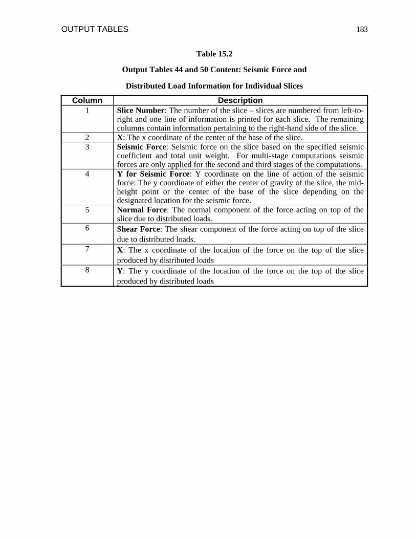
OUTPUT TABLES 183
Table 15.2
Output Tables 44 and 50 Content: Seismic Force and
Distributed Load Information for Individual Slices
Column Description 1 Slice Number: The number of the slice – slices are numbered from left-to-
right and one line of information is printed for each slice. The remaining columns contain information pertaining to the right-hand side of the slice.
2 X: The x coordinate of the center of the base of the slice. 3 Seismic Force: Seismic force on the slice based on the specified seismic
coefficient and total unit weight. For multi-stage computations seismic forces are only applied for the second and third stages of the computations.
4 Y for Seismic Force: Y coordinate on the line of action of the seismic force: The y coordinate of either the center of gravity of the slice, the mid-height point or the center of the base of the slice depending on the designated location for the seismic force.
5 Normal Force: The normal component of the force acting on top of the slice due to distributed loads.
6 Shear Force: The shear component of the force acting on top of the slice due to distributed loads.
7 X: The x coordinate of the location of the force on the top of the slice produced by distributed loads
8 Y: The y coordinate of the location of the force on the top of the slice produced by distributed loads

OUTPUT TABLES 184
Table 15.3
Output Table 45 Content: Detailed Reinforcement Force
Information for Sides and Base of Individual Slices
Column Description 1 Slice Number: The number of the slice followed by the word "Left" or
"Right" to designate the side of the slice for which the forces are being printed.
2 X: The x coordinate of the boundaries between slices. The x coordinates are printed on lines of output between the lines on which the forces are printed.
3 Horizontal Force on Side: The horizontal component of the force due to reinforcement intersecting the side (left or right) of the slice.
4 Vertical Force on Side: The vertical component of the force due to reinforcement intersecting the side (left or right) of the slice.
5 Y-Coordinate of Force: The y-coordinate of the resultant reinforcement force (due to all intersecting reinforcement) on the side of the slice.
6 Horizontal Force on Base: The horizontal component of the reinforcement force at the base of the slice (shear surface). Note: The reinforcement forces on the shear surface will always intersect the base of the slice at the left or right side because slice boundaries are positioned wherever the reinforcement lines intersect the shear surface.
7 Vertical Force on Base: The vertical component of the reinforcement force at the base of the slice (shear surface).

OUTPUT TABLES 185
Table 15.4
Output Table 46 Content: Resultant Reinforcement Forces
Assigned to Individual Slices
Column Description 1 Slice Number: The number of the slice. 2 Horizontal Force: The horizontal component of the total force on the slice
due to all reinforcement that intersects the slice. Depending on the option chosen for the reinforcement, the forces will include the reinforcement forces on the sides and base of the slice (Option 1) or only on the base of the slice (Option 2) - See Section 13 on the Group J data for internal reinforcement.
3 Vertical Force: The vertical component of the total force on the slice due to all reinforcement that intersects the slice (see note for horizontal force above regarding what forces are included).
4 Moment About Center of Slice Base: Moment produced by the reinforcement forces (in Columns 3 and 4) about the center of the base of the slice.
5 Resultant Force: Resultant force due to horizontal and vertical components shown in Columns 3 and 4.
6 Angle (degs.): Inclination of resultant force due to horizontal and vertical components shown in Columns 3 and 4 - measured in degrees from the horizontal plane; positive counter-clockwise.

OUTPUT TABLES 186
Table 15.5
Output Table 48 Content: Summary of Second-Stage Shear Strength
Computations for Individual Slices
Column Description 1 Slice Number: The number of the slice. 2 Effective Normal Stress at Consol.: Effective normal stress at
consolidation computed from the first-stage stability computations. 3 Shear Stress at Consol.: Shear stress at consolidation computed from the
first-stage stability computations. 4 Strength (Kc = 1): Shear strength computed from the "two-stage" shear
strength envelope for Kc = 1 using the effective normal stress at consolidation (in Column 2).
5 Strength (Kc = Kf): Shear strength computed from the "two-stage" shear strength envelope for Kc = Kf using the effective normal stress at consolidation (in Column 2).
6 Kc: The effective principal stress ratio at consolidation (Kc) computed from the shear and normal stresses on the shear surface (in Columns 2 and 3). If either the effective minor principal stress ratio at consolidation (Kc) or at failure (Kf) are computed to be negative, the effective principal stress ratios are not printed and an appropriate, informative message is printed in Columns 6 and 7.
7 Kf: The effective principal stress ratio at failure (Kf) computed from the effective normal stress on the shear surface and the shear strength parameters for the Kc = Kf envelope.

OUTPUT TABLES 187
Table 15.6
Output Table 52 Contents: Summary of Third-Stage Shear Strength
Computations for Individual Slices
Column Description 1 Slice Number: The number of the slice. 2 Effective Normal Stress at End of Second Stage: The effective normal
stress at the end of the second stage is computed by taking the total normal stress on the base of the slice computed in the second stage stability computations and subtracting the pore water pressure that would exist for drained conditions. The pore water pressure is computed based on the pore pressure data entered with the two-stage strength data.
3 Undrained Shear Strength: The undrained shear strength that was used for the second stage computations. These values should also be output in Output Table 49.
4 Drained Shear Strength: The "drained" shear strength calculated (estimated) using the effective normal stress in Column 2 and the effective stress shear strength parameters ( c dK Kc f= = , φ = ψK Kc f= ).
5 Strength Used: Either the word "Drained" or "Undrained" to indicate which of the two strengths (in columns 3 and 4) is lower and, thus, will subsequently be adopted for use in the third stage stability computations. The shear strengths actually used for the third-stage computations should be output in the following table (Output Table 53).

OUTPUT TABLES 188
Table 15.7
Output Table 58 Content: Final Stresses on the Shear Surface for Individual Slices
Column Description 1 Slice Number: The number of the slice – slices are numbered from left-to-
right and one line of information is printed for each slice. 2 X-Center: X coordinate of the center of the base of the slice. 3 Y_Center: Y coordinate of the center of the base of the slice. 4 Total Normal Stress: The "total" normal stress printed in this column is
actually the effective normal stress if submerged unit weights are used for the soil; otherwise the stress printed in this column is the actual total normal stress. Compression is positive; tension is negative.
5 Effective Normal Stress: The "effective" normal stress printed in this column is actually the "total" normal stress, minus any value of pore water pressure which has been defined by input data. Thus, in the case of total stress analyses, where no pore water pressures are specified, the "effective" normal stress printed in this column is actually the same as the total normal stress. Compression is positive; tension is negative.
6 Shear Stress: The shear stress on the base of the slice. The shear stress is positive when it acts on the shear surface in the direction opposite to the direction of potential sliding of the soil mass; any reasonable value of shear stress should be positive.

OUTPUT TABLES 189
Table 15.8
Output Table 59 Content: Supplemental Final Solution Information
for Spencer's Procedure
Column Description 1 Slice Number: The number of the slice – slices are numbered from left-to-
right and one line of information is printed for each slice. The remaining columns contain information pertaining to the right-hand side of the slice.
2 X-Right: The x coordinate of the right edge of the designated slice. 3 Side Force: The resultant side force on the right side of the slice.
Compressive forces are positive. 4 Y-Coord. Of Side Force Location: The y coordinate of the point of
application of the resultant side force on the right edge (vertical boundary) of the slice – the “line of thrust”.
5 Fraction of Height: The location of the side force (from Column 4) expressed as a fraction of the height of the vertical slice boundary. The value represents the height of the side force above the shear surface, expressed as a fraction of the total height of the vertical slice boundary. If the side force acts below the shear surface, the word "BELOW" is shown rather than a fractional distance; if the side force acts above the surface of the slope, the word "ABOVE" is shown.
6 Sigma at Top: The stress acting normal to the vertical slice boundary (i.e. horizontal stress) at the top of the slice. This stress is computed using the magnitude and location of the resultant side force and assuming a linear variation of stress with depth along the vertical boundary between slices. This stress is seldom of any practical use and may not be valid.
7 Sigma at Bottom: The corresponding stress at the bottom of the slice boundary determined as described for the stress in column 6. This stress is seldom of any practical use and may not be valid.

OUTPUT TABLES 190
Table 15.9
Output Table 60 Content: Supplemental Final Solution Information
for Force Equilibrium Procedures
Column Description 1 Slice Number: The number of the slice – slices are numbered from left-to-
right and one line of information is printed for each slice. The remaining columns contain information pertaining to the right-hand side of the slice.
2 X-Right: The x coordinate of the right side of the designated slice. 3 Side Force: The resultant side force on the right side of the designated
slice. Compressive forces are positive. 4 Side Force Inclination: The inclination of the side force on the right side
of the designated slice – measured in degrees from the horizontal. Positive values when the side force is inclined in a direction counter-clockwise from normal (perpendicular) to the slice boundary; negative values when the side force is inclined clockwise from the normal direction.
5 Horizontal Side Force: The horizontal component of the side force. 6 Vertical Side Force: The vertical component of the side force. Positive
side forces act down on the right side of the slice; negative forces act upwards. (The vertical side forces are computed as the product of the side force and the tangent of the side force inclination angle. Accordingly compressive side forces produce positive forces when the side force inclination is positive and negative forces when the side force inclination is negative. Negative side forces produce vertical forces with the opposite sign of positive side forces for a given inclination.)
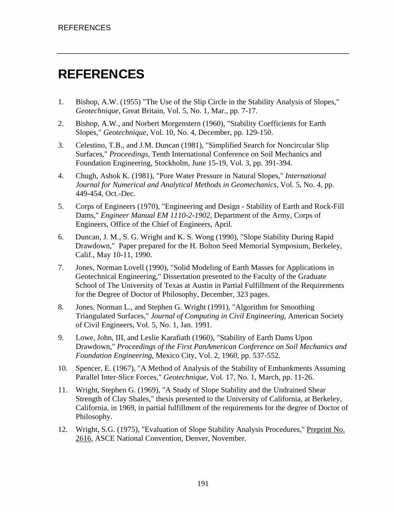
REFERENCES
191
REFERENCES
1. Bishop, A.W. (1955) "The Use of the Slip Circle in the Stability Analysis of Slopes," Geotechnique, Great Britain, Vol. 5, No. 1, Mar., pp. 7-17.
2. Bishop, A.W., and Norbert Morgenstern (1960), "Stability Coefficients for Earth Slopes," Geotechnique, Vol. 10, No. 4, December, pp. 129-150.
3. Celestino, T.B., and J.M. Duncan (1981), "Simplified Search for Noncircular Slip Surfaces," Proceedings, Tenth International Conference on Soil Mechanics and Foundation Engineering, Stockholm, June 15-19, Vol. 3, pp. 391-394.
4. Chugh, Ashok K. (1981), "Pore Water Pressure in Natural Slopes," International Journal for Numerical and Analytical Methods in Geomechanics, Vol. 5, No. 4, pp. 449-454, Oct.-Dec.
5. Corps of Engineers (1970), "Engineering and Design - Stability of Earth and Rock-Fill Dams," Engineer Manual EM 1110-2-1902, Department of the Army, Corps of Engineers, Office of the Chief of Engineers, April.
6. Duncan, J. M., S. G. Wright and K. S. Wong (1990), "Slope Stability During Rapid Drawdown," Paper prepared for the H. Bolton Seed Memorial Symposium, Berkeley, Calif., May 10-11, 1990.
7. Jones, Norman Lovell (1990), "Solid Modeling of Earth Masses for Applications in Geotechnical Engineering," Dissertation presented to the Faculty of the Graduate School of The University of Texas at Austin in Partial Fulfillment of the Requirements for the Degree of Doctor of Philosophy, December, 323 pages.
8. Jones, Norman L., and Stephen G. Wright (1991), "Algorithm for Smoothing Triangulated Surfaces," Journal of Computing in Civil Engineering, American Society of Civil Engineers, Vol. 5, No. 1, Jan. 1991.
9. Lowe, John, III, and Leslie Karafiath (1960), "Stability of Earth Dams Upon Drawdown," Proceedings of the First PanAmerican Conference on Soil Mechanics and Foundation Engineering, Mexico City, Vol. 2, 1960, pp. 537-552.
10. Spencer, E. (1967), "A Method of Analysis of the Stability of Embankments Assuming Parallel Inter-Slice Forces," Geotechnique, Vol. 17, No. 1, March, pp. 11-26.
11. Wright, Stephen G. (1969), "A Study of Slope Stability and the Undrained Shear Strength of Clay Shales," thesis presented to the University of California, at Berkeley, California, in 1969, in partial fulfillment of the requirements for the degree of Doctor of Philosophy.
12. Wright, S.G. (1975), "Evaluation of Slope Stability Analysis Procedures," Preprint No. 2616, ASCE National Convention, Denver, November.

REFERENCES 192
13. Wright, Stephen G. (1982), "Documentation for SSTAB1 - A General Computer Program for Slope Stability Analyses," Geotechnical Engineering Software GS82-1, Geotechnical Engineering Center, Bureau of Engineering Research, The University of Texas at Austin, November, 74 pages.
14. Wright, S.G., and J.D. Roecker (1984), "Example Problems for Slope Stability Computations with the Computer Program UTEXAS," Research Report 353-2, Center for Transportation Research, The University of Texas at Austin, October.
15. Wright, Stephen G. (1990), "Limit Equilibrium Slope Stability Equations Used in the Computer Program UTEXAS3," Geotechnical Engineering Software GS90-2, Geotechnical Engineering Center, Bureau of Engineering Research, The University of Texas at Austin, in press.

MULTI-STAGE STABILITY COMPUTATIONS
193
Appendix A - MULTI-STAGE STABILITY COMPUTATIONS
Introduction
Two-stage and three-stage stability computations are performed to represent conditions where the soil in a slope is allowed to first consolidate and fully "drain" and, then, is subjected to undrained loading. Two of the more common instances of such "multi-stage" loading are rapid reservoir drawdown and earthquakes.
Two-stage stability computations consist of two complete sets of stability calculations for each trial shear surface. The first set of stability computations is performed to calculate stresses along the shear surface, which represent the stresses for consolidation prior to undrained loading. These stresses are used to estimate the undrained shear strength the soil will have when it is subsequently loaded without additional drainage. The second set of stability computations is performed using the undrained shear strengths to compute the factor of safety immediately after rapid drawdown, during an earthquake or any other event that occurs rapidly enough to cause undrained loading. Different shear strengths are used for the first stage and second stage computations as described in the next sections.
Three-stage stability computations consist of as many as three complete sets of stability computations for each trial shear surface. The first two sets of stability computations are the same as those for two-stage computations. A third set of computations is performed if the undrained shear strength used in the second stage computations is greater than the shear strength that would exist if the soil were drained. In certain soils, especially those which dilate, the drained shear strength may be lower than the undrained shear strength and, thus, the drained shear strength may represent a more critical condition. The third stage of the stability computations is performed using drained shear strengths for those portions of the shear surface where the drained shear strength is lower than the undrained shear strength.
Two-stage stability computations are appropriate for earthquakes where the loads produced by the earthquake will not remain long enough for the soil to drain. Two-stage stability calculations are also used in the procedure for rapid drawdown described in the 1970 U. S. Army Corps of Engineers' slope stability manual (1970). However, for rapid drawdown, three-stage stability computations are probably more appropriate than two-stage computations (Duncan, Wright and Wong, 1990).

MULTI-STAGE STABILITY COMPUTATIONS 194
First-Stage Computations
The first set of computations in a multi-stage analysis is performed to compute the effective normal stresses and the shear stresses along the shear surface (on the base of each slice) before undrained loading. These correspond to the stresses to which the soil is consolidated before undrained loading occurs. The stresses computed from the first-stage are used to estimate undrained shear strengths, which are then used in the second set of stability computations. The first stage stability computations are performed using slope stability analysis procedures which are identical to the ones normally used to compute the factor of safety for long-term, "drained" (steady-state seepage) conditions. Effective stress shear strength properties and appropriate values of pore water pressure and external surface loads prior to undrained loading are used. In the case of rapid drawdown the external loads and pore water pressures would correspond to those that exist before drawdown. For earthquake analyses similar external loads and pore water pressures to those used for the first stage of rapid drawdown would probably be assumed for the first-stage computations.
Although a factor of safety is calculated for each trial shear surface in the first stage computations, the purpose of the computations is to compute stresses along the assumed shear surfaces; the factor of safety computed with the first stage computations is of almost no interest. The effective normal stresses on the shear surface, σfc , are calculated for individual slices from:
σfcN u= −Δ
A.1
where, N is the total normal force on the base of the slice, Δ is the length of the base of the slice, and u is the pore water pressure at the center of the base of the slice. The effective stress, σfc , is assumed to be the effective stress to which the soil is consolidated prior to undrained loading. The shear stresses on the base of each slice, τfc , are calculated from:
τfc =ΔS A.2
where, S is the shear force on the base of the slice.
Second-Stage Computations
Once the effective normal stress and shear stress are calculated for the base of each slice from the first stage computations, appropriate undrained shear strengths are determined for use in the second stage computations. The undrained shear strengths are then used to compute a factor of safety for the undrained loading due to rapid drawdown, an earthquake, etc.. The procedures used to determine the undrained shear strength are based on the procedures proposed by Duncan, Wright and Wong (1990) for stability computations for

MULTI-STAGE STABILITY COMPUTATIONS 195
rapid reservoir drawdown. The procedures for determining shear strengths for the second stage computations are also very similar to those originally recommended by Lowe and Karafiath (1960) with the further simplification that linear interpolation is used to estimate the effects of anisotropic consolidation.
"Two-Stage" Strength Envelopes
Two shear strength envelopes are used to define the shear strengths for the second stage computations (Fig. A.1). Both envelopes represent a relationship between shear strength, expressed as the shear stress on the failure plane at failure, τff , and the effective normal stress on the failure plane at consolidation, σfc . The two envelopes differ in the values of the effective principal stress ratio, Kc (= σ 1c/σ 3c) existing at the time of consolidation.
One of the shear strength envelopes used for the second-stage computations is identical to the conventional effective stress shear strength envelope, but is considered to represent the relationship between τff and σ fc for soil which is consolidated to stresses that approach (are just at) failure when the soil is consolidated, i. e. Kc = Kf, where Kf is the effective principal stress ratio at failure. This envelope is identical to the envelope normally used for long-term stability computations and the first-stage of multi-stage stability computations. The envelope plotted on a τff vs. σfc diagram is identical to the effective stress envelope plotted on a conventional Mohr-Coulomb (τ-σ ) diagram. The envelope has a slope, K Kc f
, equal to the effective stress friction angle, ψ = φ K Kc f=, and an intercept, d , equal to the effective stress cohesion value, c , for the soil.
The other shear strength envelope used for the two-stage computations is derived from results of consolidated-undrained (CU, R) type triaxial shear tests performed on specimens consolidated isotropically. This envelope corresponds to the major and minor principal stresses at consolidation being equal, i. e. Kc = 1. The envelope can be derived directly from the data from CU tests by computing and plotting ff vs. τ σfc . The shear stress on the failure plane at failure is computed from:
τff =−σ σ
φf1 3
2b g
cos
σ σ−b g
A.3
where 1 3 f is usually taken as the maximum (peak) principal stress difference and φ is the angle of internal friction expressed in terms of effective stresses. For soils whose stress-strain response does not show a pronounced peak or where a peak is reached at large strains, failure may be selected at some arbitrary, smaller value of strain, e. g. 15% axial strain. For soils which exhibit a significant reduction in strength during undrained loading it may be appropriate to use stresses less than the peak values to plot the failure envelopes. The friction angle,
σ σ1 3−b gφ , used in Eq. A.3 is identical to the friction angle from the effective stress
failure envelope. The effective stress on the failure plane, σ , which is used to plot the fc

MULTI-STAGE STABILITY COMPUTATIONS 196
Kc=1ddKc=Kf
ψKc=Kf
Kc=1ψ
σ fc
τ ff
Fig. A.1 - Shear Strength Envelopes Used to Compute Shear Strengths for Second Stage of Two-Stage Stability Computations.

MULTI-STAGE STABILITY COMPUTATIONS 197
strength envelope from CU tests, is the effective stress to which the specimens are consolidated prior to shear, i. e. σ σfc c= 3 .
The vs. τff σfc envelope for Kc = 1 can also be computed from the cohesion and friction angle, cR and φR, respectively, obtained from the "R" envelope plotted on a conventional Mohr-Coulomb diagram (Fig. A.2). The R envelope, often mistakenly referred to as the "total stress" envelope, is obtained from circles on a Mohr-Coulomb diagram, which are plotted with the effective minor principal stress being the value at consolidation, σ3c , and the principal stress difference being the principal stress difference at failure, f . Such circles do not constitute proper Mohr's circles, because one stress,
σ σ1 3−b gσ3c , is at consolidation
and the other stress, f, is at failure. However, the circles are commonly plotted and
used to determine a "total stress" (R) envelope. The envelope may be constructed either as a line drawn tangent to the circles on the Mohr-Coulomb diagram (Fig. A.3a) or as a line passing through points representing the stresses on the failure plane (Fig. A.3b); points representing stresses on the failure plane are located on the circles at an angle of
σ σ1 3−b g
φ measured counter-clockwise from the point of maximum shear stress, as shown in Fig. A.3b. The slope and intercept of the R ("total stress") envelope are expressed by a friction angle, φR, and cohesion value, cR, respectively. If the R envelope is drawn so that it is tangent to the circles (Fig. A.3a), the equations representing the corresponding slope (ψKc =1) and intercept (d ) of the τff versus
Kc =1
σfc envelope are:
d cK RR
c = =− R
FHG
IKJ1 1
cos cossin
φ φφ
A.4
and,
ψφ φ
φKR
c =−=
− R
FHG
IKJ1
1
1tan sin cos
sin A.5
If the R envelope is drawn so that it passes through points on the circles corresponding to the stresses on the failure plane (Fig. A.3b), the equations used to compute the corresponding slope (ψ ) and intercept (d ) of the τff versus σfc envelope are: Kc =1 Kc =1
d cK
Rc = =
−1 1sinR+1 tan
φφ
c h A.6
cos φ
and, ψ
φφK
Rc = =
−1 1tan
sinc hφ
φR+1cos
tan A.7
The two shear strength envelopes used to define the strengths for the second stage computations are entered as "two-stage" strengths in the input data for UTEXAS4 (See Group C Data described in Section 7 of this manual). The envelopes are entered as part of the input data for the second stage computations. Although the effective stress envelope (Kc

MULTI-STAGE STABILITY COMPUTATIONS 198
τRφ
Rc
σ3cσ
3(σ − σ )1 f
Fig. A.2 - R ("Total Stress") Envelope from Consolidated-Undrained Triaxial Shear Tests.

MULTI-STAGE STABILITY COMPUTATIONS 199
τ Rφ
Rc
σ
Fig. A.3a - R ("Total Stress") Envelope Tangent to Circles.
τ Rφ
Rcσ
φ
Fig. A.3b - R ("Total Stress") Envelope Through Points Representing Stresses on the Failure Plane.
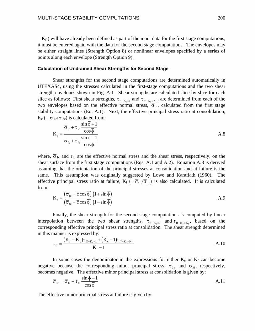
MULTI-STAGE STABILITY COMPUTATIONS 200
= Kf ) will have already been defined as part of the input data for the first stage computations, it must be entered again with the data for the second stage computations. The envelopes may be either straight lines (Strength Option 8) or nonlinear envelopes specified by a series of points along each envelope (Strength Option 9).
Calculation of Undrained Shear Strengths for Second Stage
Shear strengths for the second stage computations are determined automatically in UTEXAS4, using the stresses calculated in the first-stage computations and the two shear strength envelopes shown in Fig. A.1. Shear strengths are calculated slice-by-slice for each slice as follows: First shear strengths, τ ff Kc
and − =1 τ ff K Kf− =c, are determined from each of the
two envelopes based on the effective normal stress, σfc , calculated from the first stage stability computations (Eq. A.1). Next, the effective principal stress ratio at consolidation, Kc (= σ 1c/ 3c) is calculated from: σ
Kc
fc fc
fc fc
=+
+
+−
σ τφ
φ
σ τφ
φ
sincos
sincos
1
1 A.8
where, σ fc and τfc are the effective normal stress and the shear stress, respectively, on the shear surface from the first stage computations (Eqs. A.1 and A.2). Equation A.8 is derived assuming that the orientation of the principal stresses at consolidation and at failure is the same. This assumption was originally suggested by Lowe and Karafiath (1960). The effective principal stress ratio at failure, Kf = σ σ1 3f fb g is also calculated. It is calculated from:
Kccf
fc
fc
=+
−
+
−
σ φ
σ φ
φ
φ
coscos
sinsinc h c h
11
c h c h A.9
Finally, the shear strength for the second stage computations is computed by linear interpolation between the two shear strengths, τ ff Kc 1 and − = τ ff K Kc f
, based on the corresponding effective principal stress ratio at consolidation. The shear strength determined in this manner is expressed by:
− =
ττ τ
fff c ff K c ff K KK K K
Kc c f=
− + −
f −− = − =b g b g1 1
1 A.10
In some cases the denominator in the expressions for either Kc or Kf can become negative because the corresponding minor principal stress, σ3c and σ , respectively, becomes negative. The effective minor principal stress at consolidation is given by:
3f
σ σ τφ
φ31
c fc fc= +−sin
cos A.11
The effective minor principal stress at failure is given by:
MULTI-STAGE STABILITY COMPUTATIONS 201
σ σ φφ
φ3 2
1f fc c= −
−cos
sincos
c h c h Α.12
If either of these two stresses (σ3c or σ3f ) become zero or negative, the shear strengths are not interpolated using Eq. A.10. Instead the lower of the two shear strengths,
and , is used for the second stage stability computations. τff Kc− =1 τff K Kc f− =
Once appropriate shear strengths (τff) are determined, the shear strengths are assigned as "cohesion" values (c) for each slice and φ is set equal to zero for the second stage stability computations. Shear strengths are considered to be defined in terms of total stresses and pore water pressures are set equal to zero; actually the pore water pressure is immaterial if φ is zero.
Freely-Draining Materials
In some instances materials may be freely-draining and will not experience undrained loading even under conditions of relatively rapid loading and unloading. This may be particularly true for rapid drawdown and is less likely to be the case for earthquake loading. When materials exist, which are freely draining, the procedures used to estimate undrained strengths for the second stage of the two-stage analyses are not appropriate. The shear strengths for such materials should be represented by the same effective stress shear strength envelope and strength option (e. g. Option 1) that was used to represent the strengths for the first stage computations. Also for these materials pore water pressures representing the drained condition (after drawdown, etc.) should be specified for the second stage computations. This applies only to the materials which are freely draining.
Loading Conditions
Distributed loads and line loads for the second stage stability computations should represent the ones that will exist during and/or immediately after undrained loading. In the case of rapid drawdown the distributed loads will be the ones immediately after drawdown. In the case of earthquake loading the distributed loads for the second stage will be the ones that exist during the earthquake. The distributed loads during an earthquake might either be the same as the ones used for the first stage or be altered to reflect hydrodynamic effects.
When multi-stage stability computations are performed the seismic coefficient is only applied in the second and third stage stability computations. The seismic coefficient is not applied in the first stage of multi-stage computations13.
13 The seismic coefficient is applied in the first-stage computations when conventional, single-stage computations are performed.

MULTI-STAGE STABILITY COMPUTATIONS 202
Third-Stage Computations
Third stage computations are performed for cases where undrained shear strengths are used for the second stage computations, but the possibility exists that drainage may occur and the drained strength may be lower than the undrained strength. Three-stage stability computations are recommended for rapid drawdown, especially for materials which may dilate and become weaker as they drain.
When three-stage computations are performed, the first two stages are identical to those for two-stage computations. Once the second stage computations are completed a check is made of each slice, on a slice-by-slice basis, to determine if the drained shear strength might be lower than the undrained shear strength used in the second stage stability computations. First, the effective normal stress that would exist for drained conditions is estimated from:
σfcN u= −Δ
A.13
where N is the total normal force on the base of the slice calculated in the second stage stability computations and u is the pore water pressure that would exist once drainage and reestablishment of steady-state equilibrium has occurred following the undrained loading (rapid drawdown, earthquake, etc.). This requires that the pore water pressures that would exist after drainage has occurred be specified with the input data. This is done by specifying pore water pressures with the data for the second stage computations; the pore water pressures are ignored for the second stage computations, but used to estimate drained strengths for the third stage computations.14 The effective normal stress calculated from Eq. A.13 is used to compute the drained shear strength from the drained (effective stress) failure envelope which was entered and used for the second stage computations, i. e the vs. τff σfc envelope for Kc = Kf. If the drained shear strength is lower than the undrained shear strength that was used for the second stage stability computations, effective stress shear strength parameters ( c and φ ) and appropriate pore water pressures are assigned to the particular slice where this occurs. If the drained strength is higher than the undrained strength, the strength for the particular slice is not changed and the undrained shear strength is retained.
Once the shear strengths are checked for each slice and any changes are made in the strengths, a third set of stability computations is performed using the revised strengths. The factor of safety calculated for the third stage is then taken as the appropriate value for the trial shear surface being considered. Of course, if the drained strengths were found to be higher for all slices when checked at the end of the second stage, no third set of stability
14This applies only to materials which have been designated as having "two-stage" (undrained) strengths (Strength Options 8 and 9). Materials which will be freely drainage during an undrained loading event will have pore water pressures specified for the drained condition and the pore water pressures will be used for both the second and third stage computations for these free-draining materials.

MULTI-STAGE STABILITY COMPUTATIONS 203
computations is required and the factor if safety is the value computed in the second stage computations.
No separate sets of input data are required for three-stage computations in addition to the data entered for the second stage computations. Data for both the second and third stage computations are entered with the "second-stage" input data. When three-stage computations are performed pore water pressures representing those that would eventually exist when drainage occurs (third-stage) must be entered with the two-stage strength data (materials with shear strength Options 8 and 9 only). This may require that piezometric lines or other representations of pore water pressure be entered for the second stage even though the strength may ultimately be governed by the undrained condition and the pore water pressures may not be used directly in the final computations for the factor of safety.

EXAMPLE PROBLEMS
204
Appendix B - EXAMPLE PROBLEMS
Introduction
Three example problems are included with UTEXAS4. The first example is a simple slope that is intended to help the beginning user. If you have not used UTEXAS4 or its predecessors (UTEXAS2, UTEXAS3) before, you should begin by studying and running the first example problem. The second example is much more complex and is intended to demonstrate a large number of the features of UTEXAS4. The third example illustrates multi-stage stability computations for an embankment subjected to rapid reservoir drawdown. All computations for the example problems are performed using Spencer's procedure; Spencer's procedure is recommended for all computations. The computed factors of safety and locations of the critical shear surfaces are included in either the following text or in tables for each set of computations.
Example No. 1
Example No. 1 consists of the simple homogeneous slope illustrated in Fig. B.1. The slope is 12 feet high and has a 3(horizontal):1(vertical) side slope. The slope and its foundation consist of the same soil. The shear strength of the soil is expressed in terms of total stresses by a cohesion value (c) of 200 psf and an angle of internal friction (φ) of 22 degrees. Because total stresses are being used, no pore water pressures are specified for the computations. The unit weight of the soil is 123 lbs./cu.ft.
Stability computations are performed using circular shear surfaces. An automatic search is conducted using the Type 1, "floating grid" search scheme to locate a critical circle. The search is initiated by finding the most critical circle passing through the toe of the slope.
UTEXAS4 located the center of a critical circle at the coordinates: X = 13, Y = 32. The radius of the critical circle is 34.6 feet. The factor of safety for the critical circle is 2.74; the corresponding side force inclination (from Spencer's procedure) is 12.8 degrees.

EXAMPLE PROBLEMS 205
31
12 ft. c = 200 psfφ = 22°γ = 123 pcf
Fig. B.1 - Homogeneous Slope for Example Problem No. 1

EXAMPLE PROBLEMS 206
Example No. 2
Example No. 2 consists of the earth dam illustrated in Fig. B.2. The foundation consists of six layers of soil, underlaid by much stronger material. Seventeen (17) profile lines and thirteen (13) material types are used to characterize the cross-section of the dam and its foundation. This example is hypothetical and was developed to demonstrate a large number of the features of UTEXAS4. Accordingly, some portions of the example may not be realistic.
Three series of stability computations are performed for the second example. All computations are performed for the downstream slope. For an actual design computations would also be performed for the upstream slope, and rapid drawdown and seismic loads might also be considered.
Series 1 Computations (End-of-Construction)
The first series of computations is performed for conditions immediately after construction. No drainage is assumed to occur in the fine-grained materials; coarse-grained materials are assumed to drain freely. Shear strength properties for each of the thirteen (13) types of materials in the cross-section are summarized in Table B.1. Stability computations are performed using automatic searches with both circular and noncircular shear surfaces. The locations of the critical shear surface and the corresponding minimum factors of safety for the first series of computations (end-of-construction) are summarized in Table B.2.
No particular attempt was made to verify that the critical shear surfaces located in this series of computations are necessarily the most critical shear surfaces overall. Ordinarily additional searches would be conducted to determine if a more critical shear surface can be found.
Series 2 Computations (Steady-State Seepage)
The second series of stability computations is performed for the "long-term" stability condition with steady-state seepage established. Shear strength properties for the thirteen materials are summarized in Table B.3. Only seven of the materials (2, 3, 4, 5, 11, 12, 13) have properties which are different from those used in the first series of computations, including two materials (4 and 11) which have the same shear strength parameters, but the pore water pressure characterization is changed. The remaining six materials (1, 6, 7, 8, 9, 10) are assumed to be sufficiently permeable for "drained" shear strength properties to be used for both end-of-construction and long-term stability conditions and the pore water pressures are characterized in the same way for both

EXAMPLE PROBLEMS 207
Ri p
-rap
(7) R
ip-R
a p F
ilter
( 8)
Ups
tream
She
ll (9
)C
o re
(11)
Do w
nstre
a m S
hell
(12)
"Cap
" (13
)
Ov e
rbur
den
(6)
Ove
rbur
den
(6)
Ove
rcon
solid
ate d
Cla
y (3
)
Sh a
le (2
)
Be d
rock
(1)
Silt
y C
lay
(4)
S tiff
Cla
y (5
)
Ups
tream
Filt
er/D
rain
(10 )
Don
ws t
ream
Filt
er/D
rain
(10 )
No t
es:
1. N
umbe
rs in
par
enth
ese s
, e. g
. (11
) cor
r esp
ond
to th
e n u
mbe
rs a
ssig
ned
to
mat
e ria
ls in
the
UTE
XAS
4 d a
ta in
put f
ile.
2. T
h is
figur
e w
as p
r epa
red
usin
g Au
toC
AD L
T 97
from
Pro
f ile
Line
geo
met
r y
impo
rted
from
a D
XF fi
le c
reat
ed u
sing
Tex
Gra
f4.
T ext
labe
ling
has
been
ad
ded
in th
e C
AD s
o ftw
are.
Figu
re B
.2 -
Em
bank
me n
t Cro
ss-S
e ctio
n fo
r Exa
mp l
e N
o. 2

EXAMPLE PROBLEMS 208
TABLE B.1
Soil Properties for Example No. 2 - Short-Term, End-of-Construction Stability Condition
Mat'l
Description
Unit Weight
Shear Strength
Properties
Pore Pressure
Information 1 Lowest
foundation layer
118 pcf c = 0 psf, φ = 35° Piezometric line no. 2
2 Foundation 115 pcf Linear increase in strength with depth: su = 4000 psf at elev. of Profile Line; 5 psf increase per foot of depth.
No pore water pressures; total stresses used.
3 Foundation 122 pcf Anisotropic shear strengths - plotted in Fig. B.3
No pore water pressures; total stresses used.
4 Foundation 120 pcf c = 100 psf, φ = 27° Constant ru = 0.35 5 Foundation 125 pcf su (= c) = 4000 psf,
φ = 0
No pore water pressures; total stresses used.
6 Uppermost foundation layer
120 pcf c = 0 psf, φ = 27° Piezometric line no. 1
7 Rip-rap 125 pcf c = 0 psf, φ = 38° Piezometric line no. 1 8 Filter for rip-
rap 125 pcf c = 0 psf, φ = 34° Piezometric line no. 1
9 Upstream shell
127 pcf c = 0 psf, φ = 39° Piezometric line no. 1
10 Filters/drains for core
125 pcf c = 0 psf, φ = 33° Piezometric line no. 1
11 Core 120 pcf c = 250 psf, φ = 22° Values of ru is defined using interpolation.
12 Downstream shell
126 pcf Nonlinear shear strength envelope - plotted in Fig. B.4.
No pore water pressures; total stresses used.
13 Cap on crest 125 pcf su (c) = 1000 psf, φ = 0 No pore water pressures; total stresses used.
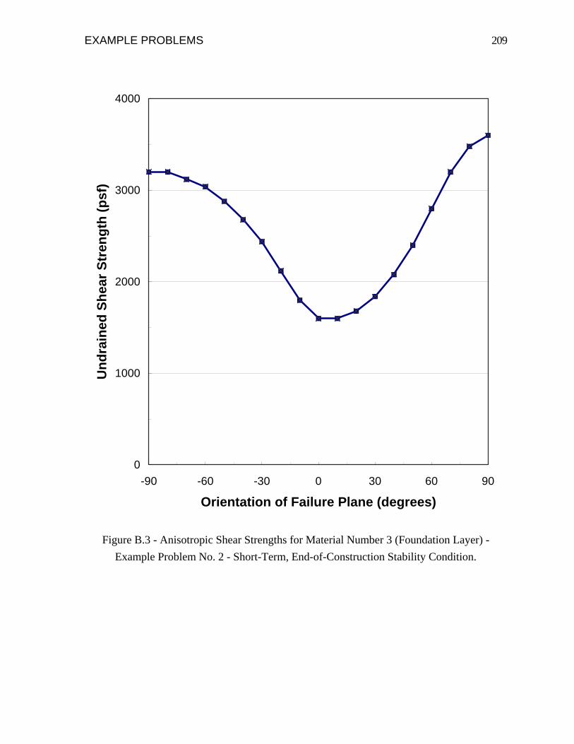
EXAMPLE PROBLEMS 209
0
1000
2000
3000
4000
-90 -60 -30 0 30 60 90
Orientation of Failure Plane (degrees)
Und
rain
ed S
hear
Str
engt
h (p
sf)
Figure B.3 - Anisotropic Shear Strengths for Material Number 3 (Foundation Layer) - Example Problem No. 2 - Short-Term, End-of-Construction Stability Condition.

EXAMPLE PROBLEMS 210
0
2000
4000
6000
8000
10000
0 5000 10000 15000 20000
Total Normal Stress (psf)
Shea
r Str
ess
(psf
)
Figure B.4 - Nonlinear Strength Envelope for Material Number 12 (Downstream Shell) - Example Problem No. 2 - Short-Term, End-of-Construction Stability Condition.

EXAMPLE PROBLEMS 211
TABLE B.2
Summary for Critical Shear Surfaces from First Series (End-Of-Construction) Stability Computations for Example No. 2
Circular Shear Surfaces (Type 1, "floating grid" search):
X coordinate for center of critical circle: 192 ft. Y coordinate for center of critical circle: 663 ft. Radius of critical circle: 238 ft. Factor of safety: 1.48 Side force inclination: -8.8 degrees
Noncircular Shear Surfaces: Coordinates of critical noncircular shear surface:
X Y -53.1 588.8 -38.9 561.0 -24.3 538.0 -4.9 500.0 12.5 475.0 41.1 450.0 58.3 433.0
130.0 425.0 267.2 433.0 304.0 450.0 331.3 475.0 384.9 500.0
Factor of safety: 1.32
Side force inclination: - 6.9 degrees

EXAMPLE PROBLEMS 212
TABLE B.3
Soil Properties for Example No. 2 - Long-Term, Steady-State Seepage Condition
Mat'l
Description Unit
Weight
Shear Strength Properties
Pore Pressure
Information 1 Lowest
foundation layer
118 pcf c = 0 psf, φ = 35° Piezometric line no. 2
2 Foundation 115 pcf c = 0 psf, φ = 26° Pore water pressures defined using interpolation.
3 Foundation 122 pcf c = 0 psf, φ = 16° Constant pore water pressures = 7000 psf.
4 Foundation 120 pcf c = 100 psf, φ = 27° Pore water pressures defined using interpolation.
5 Foundation 125 pcf c = 500 psf, φ = 24° Pore water pressures defined using interpolation.
6 Uppermost foundation layer
120 pcf c = 0 psf, φ = 27° Piezometric line no. 1
7 Rip-rap 125 pcf c = 0 psf, φ = 38° Piezometric line no. 1 8 Filter for
rip-rap 125 pcf c = 0 psf, φ = 34° Piezometric line no. 1
9 Upstream shell
127 pcf c = 0 psf, φ = 39° Piezometric line no. 1
10 Filters/drains for core
125 pcf c = 0 psf, φ = 33° Piezometric line no. 1
11 Core 120 pcf c = 250 psf, φ = 22° Pore water pressures defined using interpolation; negative pore pressures allowed.
12 Downstream shell
126 pcf c = 200 psf, φ = 29° Zero pore water pressures.
13 Cap on crest 125 pcf c = 0 psf, φ = 25° Piezometric line no. 1
EXAMPLE PROBLEMS 213
conditions. For these six materials (1, 6, 7, 8, 9, 10) the material property data for long-term stability computations is identical to the data for the short-term stability computations; only the pore water pressures (piezometric levels) are changed.
An automatic search is performed using noncircular shear surfaces only. Again, the critical shear surface located for these example computations may not represent the most critical shear surface. Additional searches with different starting locations and shapes would need to be tried to verify the location of the most critical shear surface. Results of the second series of stability computations are summarized in Table B.4 along with the results of the third series of computations described below.
Series 3 Computations (Steady-State Seepage with Berm)
The third series of stability computations is performed for the long-term, steady-state seepage condition with a berm added at the downstream side of the dam. Properties of the berm material are as follows:
Total unit weight, γ = 125 pcf
Cohesion, c = 0
Friction angle, φ = 35 degrees
The berm material is assumed to be freely draining and the pore water pressures in the berm are assumed to be zero. All other materials are assumed to have the same properties as shown earlier in Table B.3. The critical shear surface and the corresponding minimum factor of safety for the third series of computations are summarized in Table B.4.

EXAMPLE PROBLEMS 214
TABLE B.4
Summary of Second and Third Series (Steady-State Seepage) Stability Computations for Example No. 2
Second Series: Noncircular Shear Surfaces (No Berm): Coordinates of critical noncircular shear surface:
X Y -58.7 586.5 -44.0 557.2 -26.6 522.6 -11.0 500.0 12.4 475.0 45.8 450.0 67.3 433.0
190.6 425.0 289.4 433.0 342.4 450.0 394.2 475.0 444.4 500.0
Factor of safety: 1.09 Side force inclination: - 8.8 degrees
Third Series: Noncircular Shear Surfaces (With Berm): Coordinates of critical noncircular shear surface:
X Y -61.5 585.4 -42.4 556.6 -26.6 523.0 -9.9 500.0 12.3 475.0 42.6 450.0 65.5 433.0
111.9 425.0 603.8 433.0 651.0 450.0 696.8 475.0 740.0 500.0
Factor of safety: 1.46 Side force inclination: - 5.9 degrees

EXAMPLE PROBLEMS 215
Example No. 3
Example No. 3 is a hypothetical zoned earth embankment. A cross-section is shown in Fig. B.5 The embankment and foundation are represented using ten (10) Profile Lines and nine (9) different materials. Three-stage stability computations are performed for an assumed drawdown from elevation 545 to 380. Material properties for the first-stage computations are presented in Table B.5; material properties for the second and third stage computations are in Table B.6.
Stability computations are performed using the Type 1, "floating grid" search scheme with circular shear surfaces. Results of the stability computations are summarized in Table B.7.
The critical shear surface located for the example computations may not represent the most critical shear surface. Additional searches with different starting locations and shapes of shear surfaces would need to be tried to verify the location of the most critical shear surface.

EXAMPLE PROBLEMS 216
Foun
datio
n R
ock
(1)
Ove
rbur
d en
(2)
Ups
tream
She
ll (6
)
Ran
dom
Zon
e (3
)
Ups
tream
Fi lt
erA
bove
Dr a
wdo
wn
(5)
Ups
tr eam
Filt
erB
e low
Dra
wdo
wn
(4)
Cor
e (7
)
Dow
n stre
am F
i lter
(8)
Dow
nstre
am S
hell
(9)
Not
e s:
1. N
umb e
rs in
pa r
enth
eses
, e. g
. (7)
cor
resp
o nd
to n
umbe
rs
assi
gne d
to m
ate r
ials
in th
e U
TEX
A S4
data
inpu
t file
.2 .
The
dra
win
g w
as p
repa
red
usin
g A
u toC
AD
LT
97 fr
om P
rofil
e L i
ne g
eom
etry
impo
rted
from
a D
XF
file
crea
ted
usin
g Te
x Gra
f4.
Text
labe
li ng
was
add
e d in
the
CA
D s
oftw
are.
F igu
re B
.5 -
Em
bank
men
t Cr o
ss-S
e ctio
n fo
r Exa
mpl
e N
o . 3

EXAMPLE PROBLEMS 217
TABLE B.5
Soil Properties for Example No. 3 First-Stage of Rapid Drawdown Stability Computations
Mat'l
Description Unit
Weight Shear Strength
Properties Pore Pressure
Information 1 Foundation
rock 125 pcf "Very Strong" Not applicable
2 Foundation overburden
125 pcf c = 400 psf, φ = 38° Piezometric line no. 1
3 Random zone upstream
140 pcf c = 0 psf, φ = 36° Piezometric line no. 1
4, 5 Upstream filter
142 pcf c = 0 psf, φ = 35° Piezometric line no. 1
6 Upstream shell
142 pcf c = 0 psf, φ = 37° Piezometric line no. 1
7 Central core 140 pcf Nonlinear strength envelope
(See Fig. B.6)
Piezometric line no. 1
σ τ 0 0 1100 1100 1250 1150 3250 2200 20000 13500 8 Downstream
filter 128 pcf c = 0 psf, φ = 35° Piezometric line no. 1
9 Downstream shell
128 pcf c = 0 psf, φ = 37° Piezometric line no. 1

EXAMPLE PROBLEMS 218
0
5000
10000
15000
20000
0 5000 10000 15000 20000
Effective Normal Stress (psf)
Shea
r Str
ess
(psf
)
Fig. B.6 - Nonlinear Shear Strength Envelope for Material No. 7 (Central Core) for First Stage Computations - Example No. 3.

EXAMPLE PROBLEMS 219
TABLE B.6
Soil Properties for Example No. 3 Second and Third Stages of Rapid Drawdown Stability Computations
Mat'l
Description
Unit Weight
Shear Strength Properties
Pore Pressure
Information 1 Foundation
rock 125 pcf "Very Strong" Not applicable
2 Foundation overburden
125 pcf 2-Stage, strengths; linear envelope: dKc =1 = 900 psf; ψKc =1
dK Kc f=
= 32°; (=c ) = 400 psf;
ψK Kc f= (=φ ) = 38°
Piezometric line no. 1
3 Random zone upstream
140 pcf 2-Stage, strengths; linear envelope: dKc =1 = 3000 psf; ψKc =1
d = 22°;
K Kc = f (= c ) = 0 psf;
ψKc =1 (= φ ) = 37°
Piezometric line no. 1
4 Upstream filter - below drawdown
142 pcf c = 0 psf, φ = 35° Piezometric line no. 1
5 Upstream filter - above drawdown
128 pcf c = 0 psf, φ = 35° Piezometric line no. 1
6 Upstream shell
128 pcf c = 0 psf, φ = 37° Piezometric line no. 1
7 Central core 140 pcf Nonlinear strength envelope (See Fig. B.7)
Piezometric line no. 1
sfc τff Kc− =1 τff K Kc f− =
-10000 0 0 0 0 0 1100 700 1100 1250 800 1150 3250 1350 2200 20000 5800 13500 8 Downstream
filter 128 pcf c = 0 psf, φ = 35° Piezometric line
no. 1 9 Downstream
shell 128 pcf c = 0 psf, φ = 37° Piezometric line
no. 1

EXAMPLE PROBLEMS 220
0
5000
10000
15000
20000
0 5000 10000 15000 20000
Effective Consolidation Stress (psf)
Shea
r Str
ess
at F
ailu
re (p
sf)
Kc = 1Kc = Kf
Fig. B.7 - Nonlinear Shear Strength Envelopes for Material No. 7 (Central Core) for Second Stage Computations - Example No. 3.
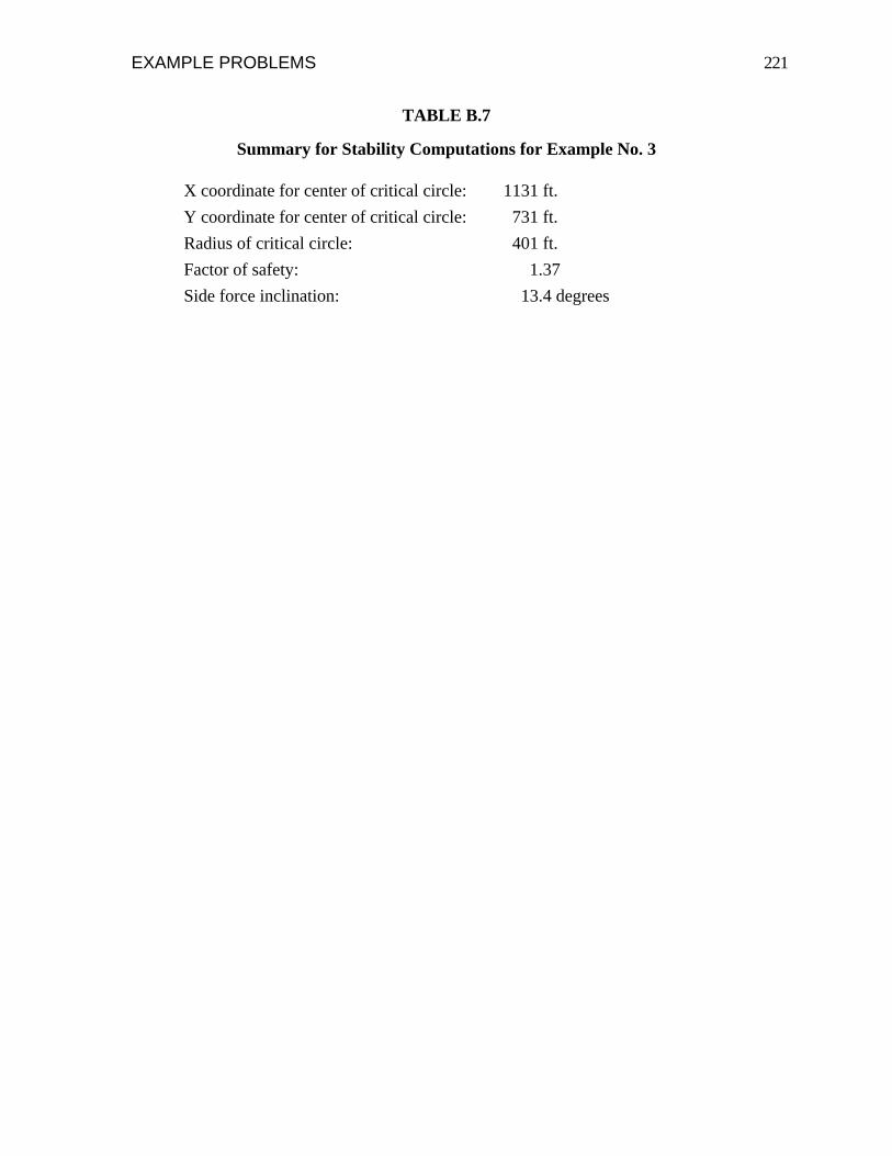
EXAMPLE PROBLEMS 221
TABLE B.7
Summary for Stability Computations for Example No. 3
X coordinate for center of critical circle: 1131 ft. Y coordinate for center of critical circle: 731 ft. Radius of critical circle: 401 ft. Factor of safety: 1.37 Side force inclination: 13.4 degrees