TA Lecture 12 Compression.pptx - ut · TextAlgorithms%(6EAP)% % Compression% Jaak%Vilo% 2010%fall%...

Text Algorithms (6EAP)

Compression

Jaak Vilo 2010 fall

1 MTAT.03.190 Text Algorithms Jaak Vilo

Problem

•  Compress – Text –  Images, video, sound, …

•  Reduce space, efficient communicaMon, etc… – Data deduplicaMon

•  Exact compression/decompression •  Lossy compression

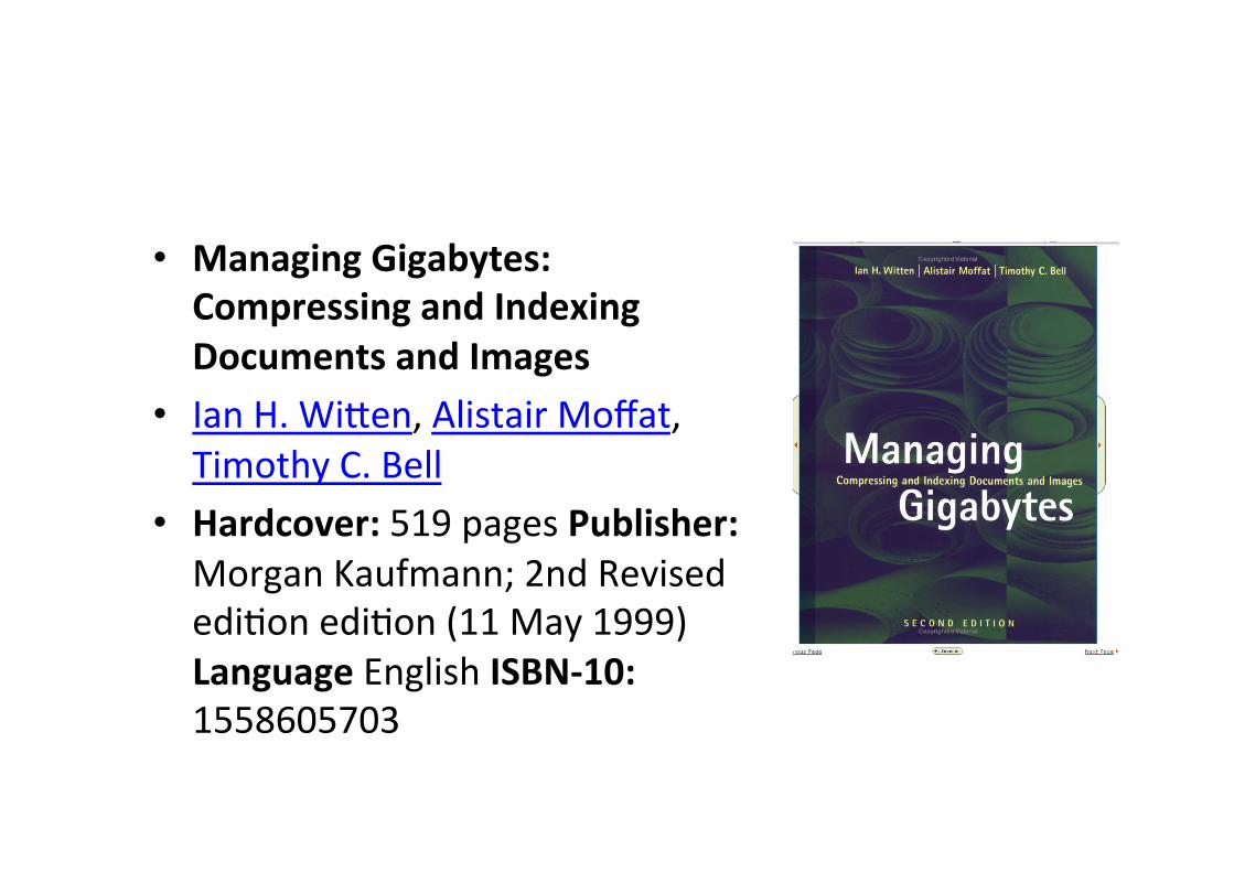
•  Managing Gigabytes: Compressing and Indexing Documents and Images

•  Ian H. WiTen, Alistair Moffat, Timothy C. Bell

•  Hardcover: 519 pages Publisher: Morgan Kaufmann; 2nd Revised ediMon ediMon (11 May 1999) Language English ISBN-‐10: 1558605703

Links

•  hTp://datacompression.info/ •  hTp://en.wikipedia.org/wiki/Data_compression

•  Data Compression Debra A. Lelewer and Daniel S. Hirschberg –  hTp://www.ics.uci.edu/~dan/pubs/DataCompression.html

•  Compression FAQ hTp://www.faqs.org/faqs/compression-‐faq/

•  InformaMon Theory Primer With an Appendix on Logarithms by Tom Schneider hTp://www.lecb.ncifcrf.gov/~toms/paper/primer/

•  hTp://www.cbloom.com/algs/index.html

Problem •  InformaMon transmission •  InformaMon storage •  The data sizes are huge and growing

–  fax -‐ 1.5 x 106 bit/page –  photo: 2M pixels x 24bit = 6MB –  X-‐ray image: ~ 100 MB? –  Microarray scanned image: 30-‐100 MB –  Tissue-‐microarray -‐ hundreds of images, each tens of MB –  Large Hardon Collider (CERN) -‐ The device will produce few peta (1015) bytes of stored

data in a year. –  TV (PAL) 2.7 ·∙ 108 bit/s –  CD-‐sound, super-‐audio, DVD, ...

–  Human genome – 3.2Gbase. 30x sequencing => 100Gbase + quality info (+ raw data) –  1000 genomes, all individual genomes …

What it’s about? •  EliminaMon of redundancy •  Being able to predict… •  Compression and decompression

–  Represent data in a more compact way –  Decompression -‐ restore original form

•  Lossy and lossless compression –  Lossless -‐ restore in exact copy –  Lossy -‐ restore almost the same informaMon

•  Useful when no 100% accuracy needed •  voice, image, movies, ... •  Decompression is determinisMc (lossy in compression phase) •  Can achieve much more effecMve results

Methods covered:

•  Code words (Huffman coding) •  Run-‐length encoding •  ArithmeMc coding •  Lempel-‐Ziv family (compress, gzip, zip, pkzip, ...) •  Burrows-‐Wheeler family (bzip2) •  Other methods, including images •  Kolmogorov complexity •  Search from compressed texts

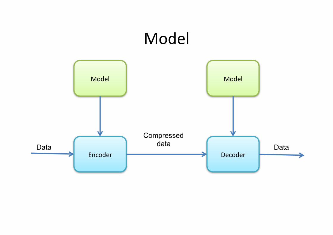
Model

Encoder Decoder

Model Model

Data Data

Compressed data

•  Let pS be a probability of message S •  The informaMon content can be represented in terms of bits •  I(S) = -‐log( pS ) bits •  If the p=1 then the informaMon content is 0 (no new

informaMon) –  If Pr[s]=1 then I(s) = 0. –  In other words, I(death)=I(taxes)=0

•  I( heads or tails ) = 1 -‐-‐ if the coin is fair •  Entropy H(S) is the average informaNon content of S

–  H(S) = pS ·∙ I(S) = -‐pS log( pS ) bits

hTp://en.wikipedia.org/wiki/InformaMon_entropy

•  Shannon's experiments with human predictors show an informaMon rate of between .6 and 1.3 bits per character, depending on the experimental setup; the PPM compression algorithm can achieve a compression raMo of 1.5 bits per character.

•  No compression can on average achieve beTer compression than the entropy

•  Entropy depends on the model (or choice of symbols) •  Let M={ m1, .. mn } be a set of symbols of the model A and let

p(mi) be the probability of the symbol mi •  The entropy of the model A, H(M) is -‐∑i=1..n p(mi) ·∙ log( p(mi) )

bits •  Let the message S = s1, .. sk, and every symbol si be in the

model M. The informaMon content of model A is -‐∑i=1..k log p(si)

•  Every symbol has to have a probability, otherwise it cannot be coded if it is present in the data

hTp://marknelson.us/2006/08/24/the-‐huTer-‐prize/#comment-‐293

•  The data compression world is all abuzz about Marcus HuTer’s recently announced 50,000 euro prize for record-‐breaking data compressors. Marcus, of the Swiss Dalle Molle InsMtute for ArMficial Intelligence, apparently in cahoots with Florida compression maven MaT Mahoney, is offering cash prizes for what amounts to the most impressive ability to compress 100 MBytes of Wikipedia data. (Note that nobody is going to win exactly 50,000 euros -‐ the prize amount is prorated based on how well you beat the current record.)

•  This prize differs considerably from my Million Digit Challenge, which is really nothing more than an aTempt to silence people foolishly claiming to be able to compress random data. Marcus is instead looking for the most effecMve way to reproduce the Wiki data, and he’s pu|ng up real money as an incenMve. The benchmark that contestants need to beat is that set by MaT Mahoney’s paq8f , the current record holder at 18.3 MB. (Alexander Ratushnyak’s submission of a paq variant looks to clock in at a Mdy 17.6 MB, and should soon be confirmed as the new standard.)

•  So why is an AI guy inserMng himself into the world of compression? Well, Marcus realizes that good data compression is all about modeling the data. The beTer you understand the data stream, the beTer you can predict the incoming tokens in a stream. Claude Shannon empirically found that humans could model English text with an entropy of 1.1 to 1.6 0.6 to 1.3 bits per character, which at at best should mean that 100 MB of Wikipedia data could be reduced to 13.75 7.5 MB, with an upper bound of perhaps 20 16.25 MB. The theory is that reaching that 7.5 MB range is going to take such a good understanding of the data stream that it will amount to a demonstraMon of ArMficial Intelligence.

http://prize.hutter1.net/

Model

Encoder Decoder

Model Model

Data Data

Compressed data

StaMc or adapMve

•  StaMc model does not change during the compression

•  AdapMve model can be updated during the process •  Symbols not in message cannot have 0-‐probability •  Semi-‐adapMve model works in 2 stages, off-‐line. •  First create the code table, then encode the message with the code table

How to compare compression techniques?

•  RaMo (t/p) t: original message length •  p: compressed message length •  In texts -‐ bits per symbol •  The Mme and memory used for compression •  The Mme and memory used for decompression

•  error tolerance (e.g. self-‐correcMng code)

Shorter code words…

•  S = 'aa bbb cccc ddddd eeeeee fffffffgggggggg' •  Alphabet of 8 •  Length = 40 symbols •  Equal length codewords

•  3-‐bit a 000 b 001 c 010 d 011 e 100 f 101 g 110 space 110

•  S compressed -‐ 3*40 = 120 bits

Run-‐length encoding •  hTp://michael.dipperstein.com/rle/index.html •  The string:

•  "aaaabbcdeeeeefghhhij"

•  may be replaced with

•  "a4b2c1d1e5f1g1h3i1j1". •  This is not shorter because 1-‐leTer repeat takes more characters... •  "a3b1cde4fgh2ij" •  Now we need to know which characters are followed by run-‐length. •  E.g. use escape symbols. •  Or, use the symbol itself -‐ if repeated, then must be followed by run-‐

length •  "aa2bb0cdee3fghh1ij"

AlphabeNcally ordered word-‐lists

resume retail retain retard retire

0resume 2tail 5n 4rd 3ire

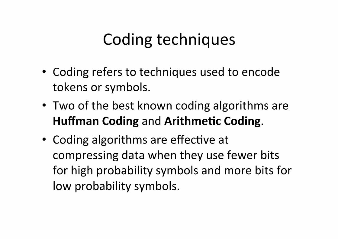
Coding techniques

•  Coding refers to techniques used to encode tokens or symbols.

•  Two of the best known coding algorithms are Huffman Coding and ArithmeNc Coding.

•  Coding algorithms are effecMve at compressing data when they use fewer bits for high probability symbols and more bits for low probability symbols.

Variable length encoders

•  How to use codes of variable length? •  Decoder needs to know how long is the symbol

•  Prefix-‐free code: no code can be a prefix of another code

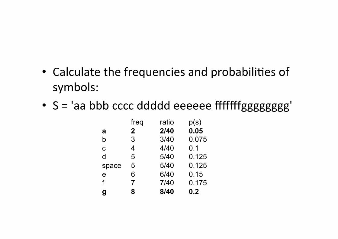
•  Calculate the frequencies and probabiliMes of symbols:

•  S = 'aa bbb cccc ddddd eeeeee fffffffgggggggg'

freq ratio p(s) a 2 2/40 0.05 b 3 3/40 0.075 c 4 4/40 0.1 d 5 5/40 0.125 space 5 5/40 0.125 e 6 6/40 0.15 f 7 7/40 0.175 g 8 8/40 0.2

Algoritm Shannon-‐Fano

•  Input: probabiliMes of symbols •  Output: Codewords in prefix free coding

1. Sort symbols by frequency 2. Divide to two almost probable groups 3. First group gets prefix 0, other 1 4. Repeat recursively in each group unMl 1 symbol remains

Example 1

a 1/2 0 b 1/4 10 c 1/8 110 d 1/16 1110 e 1/32 11110 f 1/32 11111

Example 1

a 1/2 0 b 1/4 10 c 1/8 110 d 1/16 1110 e 1/32 11110 f 1/32 11111

Code:

Shannon-‐Fano S = 'aa bbb cccc ddddd eeeeee fffffffgggggggg'

p(s) code

g 0.2 00 f 0.175 010 e 0.15 011 d 0.125 100 space 0.125 101 c 0.1 110 b 0.075 1110 a 0.05 1111

1

0.475

0.525 0.2

0.325 0.15

0.175

Shannon-‐Fano

•  S = 'aa bbb cccc ddddd eeeeee fffffffgggggggg' •  S in compressed is 117 bits •  2*4 + 3*4 + 4*3 + 5*3 + 5*3 + 6*3 + 7*3 + 8*2 = 117

•  Shannon-‐Fano not always opMmal •  SomeMmes 2 equal probable groups cannot be achieved

•  Usually beTer than H+1 bits per symbol, when H is entropy.

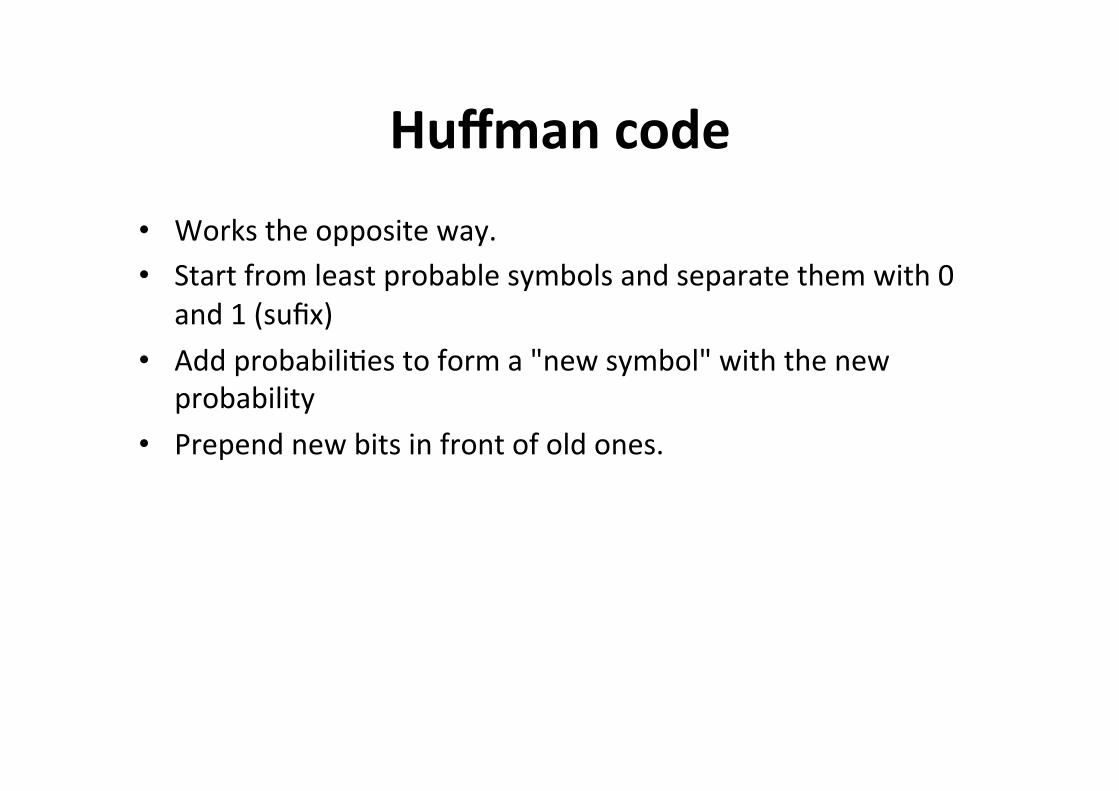
Huffman code •  Works the opposite way. •  Start from least probable symbols and separate them with 0

and 1 (sufix) •  Add probabiliMes to form a "new symbol" with the new

probability •  Prepend new bits in front of old ones.

Huffman example Char Freq Code space 7 111 a 4 010 e 4 000 f 3 1101 h 2 1010 i 2 1000 m 2 0111 n 2 0010 s 2 1011 t 2 0110 l 1 11001 o 1 00110 p 1 10011 r 1 11000 u 1 00111 x 1 10010 "this is an example of a huffman tree"

•  Huffman coding is opMmal when the frequencies of input characters are powers of two. ArithmeMc coding produces slight gains over Huffman coding, but in pracMce these gains have not been large enough to offset arithmeMc coding's higher computaMonal complexity and patent royalMes

•  (as of November 2001/Jul2006, IBM owns patents on the core concepts of arithmeMc coding in several jurisdicMons). hTp://en.wikipedia.org/wiki/ArithmeMc_coding#US_patents_on_arithmeMc_coding

ProperNes of Huffman coding

•  Error tolerance quite good •  In case of the loss, adding or change of a single bit, the differences remain local to the place of the error

•  Error usually remains quite local (proof?) •  Has been shown, the code is opMmal •  Can be shown the average result is H+p+0.086, where H is the entropy and p is the probability of the most probable symbol

Move to Front

•  Move to Front (MTF), Least recently used (LRU)

•  Keep a list of last k symbols of S •  Code

– use the code for symbol. –  if in codebook, move to front –  if not in codebook, move to first, remove the last

•  c.f. the handling of memory paging •  Other heurisMcs ...

ArithmeNc (en)coding •  ArithmeMc coding is a method for lossless data compression. •  It is a form of entropy encoding, but where other entropy encoding

techniques separate the input message into its component symbols and replace each symbol with a code word, arithmeMc coding encodes the enMre message into a single number, a fracMon n where (0.0 n < 1.0).

•  Huffman coding is opMmal for character encoding (one character-‐one code word) and simple to program. ArithmeMc coding is beTer sMll, since it can allocate fracMonal bits, but more complicated.

•  Wikipedia hTp://en.wikipedia.org/wiki/ArithmeMc_encoding •  EnMre message is a single floaMng point number, a fracMon n where (0.0 n

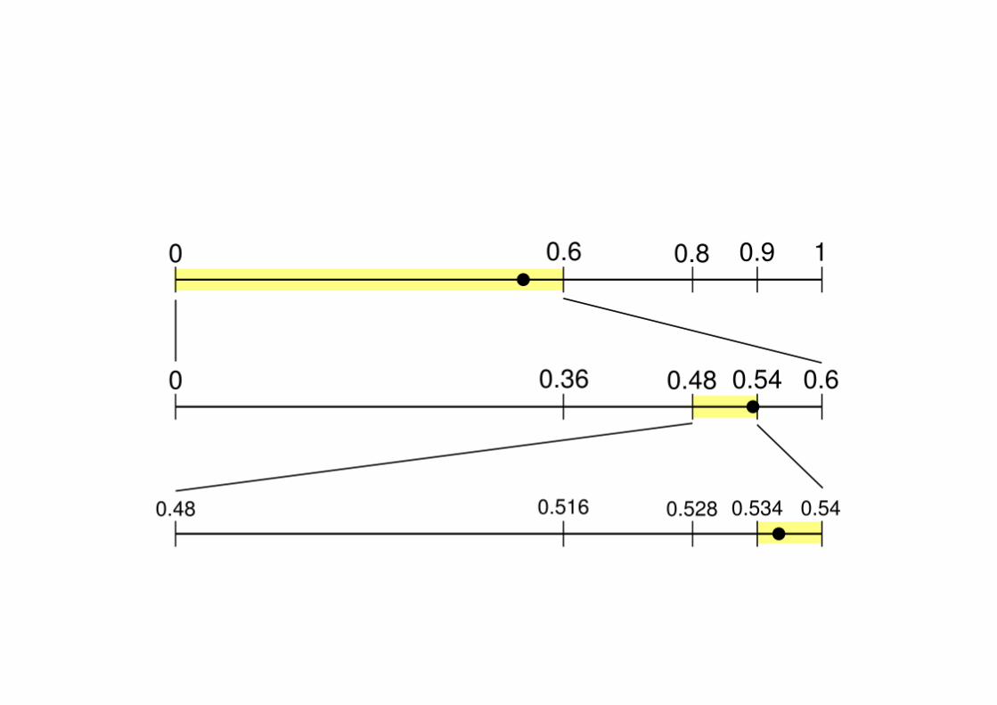
< 1.0). •  Every symbol gets a probability based on the model •  ProbabiliMes represent non-‐intersecMng intervals •  Every text is such an interval

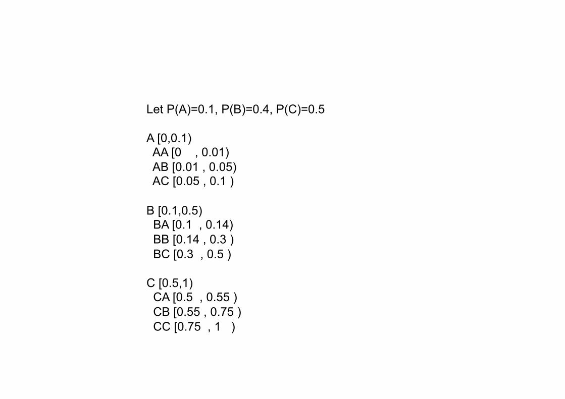
Let P(A)=0.1, P(B)=0.4, P(C)=0.5 A [0,0.1) AA [0 , 0.01) AB [0.01 , 0.05) AC [0.05 , 0.1 ) B [0.1,0.5) BA [0.1 , 0.14) BB [0.14 , 0.3 ) BC [0.3 , 0.5 ) C [0.5,1) CA [0.5 , 0.55 ) CB [0.55 , 0.75 ) CC [0.75 , 1 )

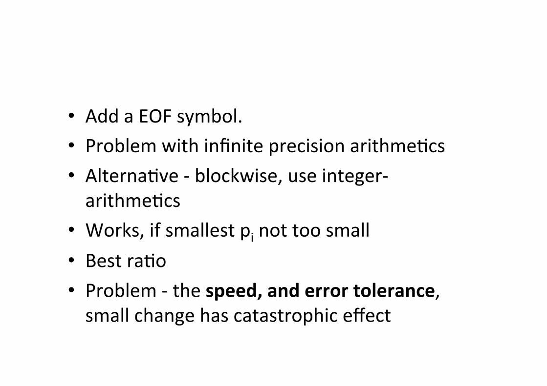
•  Add a EOF symbol. •  Problem with infinite precision arithmeMcs •  AlternaMve -‐ blockwise, use integer-‐arithmeMcs

•  Works, if smallest pi not too small •  Best raMo •  Problem -‐ the speed, and error tolerance, small change has catastrophic effect

•  Invented by Jorma Rissanen (then at IBM) •  ArithmeMc coding revisited by Alistair Moffat, Radford M.

Neal, Ian H. WiTen -‐ hTp://portal.acm.org/citaMon.cfm?id=874788

•  Models for arithmeMc coding -‐ •  HMM Hidden Markov Models •  ... •  Context methods: Abrahamson dependency model •  Use the context to maximum, to predict the next symbol •  PPM -‐ PredicMon by ParMal Matching •  Several contexts, choose best •  VariaMons

DicNonary based compression

•  DicMonary (symbol table) , list codes •  If not in discMonary, use escape •  Usual heurisMcs searches for longest repeat •  With fixed table one can search for opMmal code

•  With adapMve dicMonary the opMmal coding is NP-‐complete

•  Quite good for English language texts, for example

Lempel-‐Ziv family, LZ, LZ-‐77 •  Use the dicMonary to memorise the previously compressed parts •  LZ-‐77 •  Sliding window of previous text; and text to be compressed

/bbaaabbbaaffacbbaa…./...abbbaabab... •  Lookahead -‐ longest prefix that begins within the moving window, is

encoded with [posiMon,length] •  In example, [5,6] •  Fast! (Commercial so�ware, e.g. PKZIP, Stacker, DoubleSpace, ) •  Several alternaMve codes for same string (alternaMve substrings will match) •  Lempel-‐Ziv compression from McGill Univ.

hTp://www.cs.mcgill.ca/~cs251/OldCourses/1997/topic23/

Original LZ77 •  Triples [posiMon,length,next char] •  If output [a,b,c], advance by b+1 posiMons •  For each part of the triple the nr of bits is reserved depending on window length

⎡ log(n-‐f) ⎤ + ⎡ log(f) ⎤ + 8 where n is window size, and f is lookahead size

•  Example: abbbbabbc [0,0,a] [0,0,b] [1,3,a] [3,2,c]

•  In example the match actually overlaps with lookahead window

LZ-‐78 •  DicNonary •  Store strings from processed part of the message •  Next symbol is the longest match from dicMonary, that

matches the text to be processed •  LZ78 (Ziv and Lempel 1978) •  First, dicMonary is empty, with index 0 •  Code [i,c] -‐ refers to dicMonary (word u at pos. i) and c is the

next symbol •  Add uc to dicMonary •  Example: ababcabc → [0,a][0,b][1,b][0,c][3,c]

LZW

•  Code consists of indices only! •  First, dicMonary has every symbol /alphabet/ •  Update dicMonary like LZ78 •  In decoding there is a danger: See abcabca

–  If abc is in dicMonary –  add abca to dicMonary –  next is abca, output that code

–  But when decoding, aaer abc it is not known that abca is in the dicNonary

•  SoluMon -‐ if the dicMonary entry is used immediately a�er its creaMon, the 1st and last characters have to match

•  Many representaMons for the dicMonary. •  List, hash, sorted list, combinaMon, binary tree, trie, suffix tree, ...

LZJ

•  Coding -‐ search for longest prefix. •  Code -‐ address of the trie node •  From the root of the trie, there is a transiMon on every symbol (like in LZW).

•  If out of memory, remove these nodes/branches that have been used only once

•  In pracMce, h=6, dicMonary has 8192 nodes

LZFG

•  EffecMve LZ method •  From LZJ •  Create a suffix tree for the window •  Code -‐ node address plus nr of characters from teh edge.

•  The internal and leaf nodes with different codes

•  small match directly... (?)

Burrows-‐Wheeler •  See FAQ hTp://www.faqs.org/faqs/compression-‐faq/part2/secMon-‐9.html •  The method described in the original paper is really a composite of three different

algorithms: –  the block sorMng main engine (a lossless, very slightly expansive preprocessor), –  the move-‐to-‐front coder (a byte-‐for-‐byte simple, fast, locally adapMve noncompressive coder) and –  a simple staMsMcal compressor (first order Huffman is menMoned as a candidate) eventually doing

the compression.

•  Of these three methods only the first two are discussed here as they are what consMtutes the heart of the algorithm. These two algorithms combined form a completely reversible (lossless) transformaMon that -‐ with typical input -‐ skews the first order symbol distribuMons to make the data more compressible with simple methods. IntuiMvely speaking, the method transforms slack in the higher order probabiliMes of the input block (thus making them more even, whitening them) to slack in the lower order staMsMcs. This effect is what is seen in the histogram of the resulMng symbol data.

•  Please, read the arMcle by Mark Nelson: •  Data Compression with the Burrows-‐Wheeler Transform Mark Nelson, Dr. Dobb's Journal

September, 1996. hTp://marknelson.us/1996/09/01/bwt/

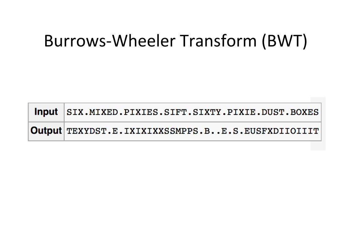
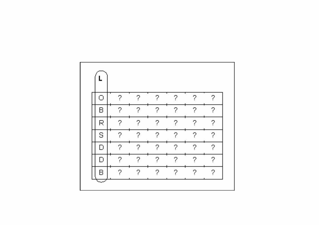
Burrows-‐Wheeler Transform (BWT)

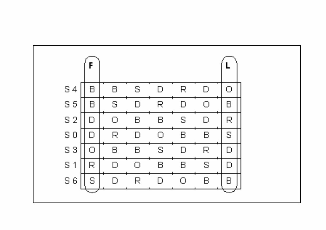
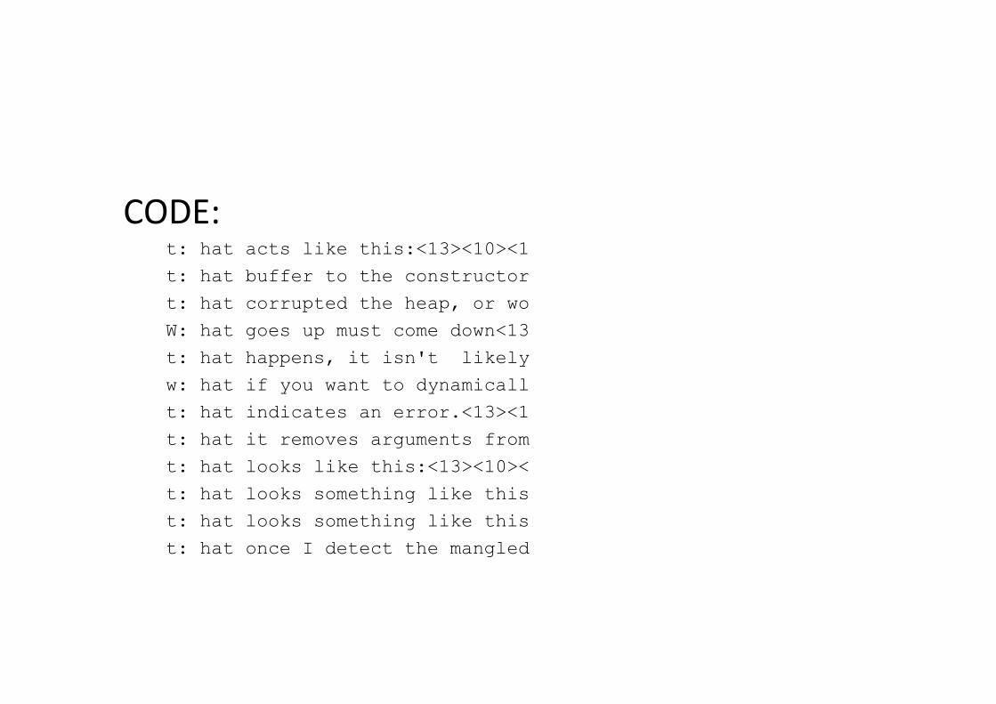
CODE: t: hat acts like this:<13><10><1

t: hat buffer to the constructor

t: hat corrupted the heap, or wo

W: hat goes up must come down<13

t: hat happens, it isn't likely

w: hat if you want to dynamicall

t: hat indicates an error.<13><1

t: hat it removes arguments from

t: hat looks like this:<13><10><

t: hat looks something like this

t: hat looks something like this

t: hat once I detect the mangled

Example

•  Decode: errktreteoe.e

•  Hint: . Is the last character, alphabeMcally first…

SyntacNc compression

•  Context Free Grammar for presenMng the syntax tree

•  Usually for source code •  AssumpMon -‐ program is syntacMcally correct •  Comments •  Features, constants -‐ group by group

Image compression

•  Many images, photos, sound, video, ...

Fax group 3

•  Fax/group 3 •  Black/white, 0/1 code •  Run-‐length: 000111001000 → 3,3,2,1,3 •  Variable-‐length codes for represenMng run-‐lengths.

•  Joint Photographic Experts Group JPEG 2000 hTp://www.jpeg.org/jpeg2000/

•  Image Compression -‐-‐ JPEG from W.B. Pennebaker, J.L. Mitchell, "The JPEG SMll Image Data Compression Standard", Van Nostrand Reinhold, 1993.

•  Color image, 8 or 12 bits per pixel per color. •  Four modes SequenMal Mode •  Lossless Mode •  Progressive Mode •  Hierarchical Mode •  DCT (Discrete Cosine Transform)

•  from hTp://www.utdallas.edu/~aria/mcl/post/ •  Lossy signal compression works on the basis of transmi|ng the "important" signal

content, while omi|ng other parts (QuanMzaMon). To perform this quanMzaMon effecMvely, a linear de-‐correlaMng transform is applied to the signal prior to quanMzaMon. All exisMng image and video coding standards use this approach. The most commonly used transform is the Discrete Cosine Transform (DCT) used in JPEG, MPEG-‐1, MPEG-‐2, H.261 and H.263 and its descendants. For a detailed discussion of the theory behind quanMzaMon and jusMficaMon of the usage of linear transforms, see reference [1] below.

•  A brief overview of JPEG compression is as follows. The JPEG encoder parMMons the image into 8x8 blocks of pixels. To each of these blocks it applies a 2-‐dimensional DCT. The transform matrix is normalized (element-‐wise) by a 8x8 quanMzaMon matrix and then rounded to the nearest integer. This operaMon is equivalent to applying different uniform quanMzers to different frequency bands of the image. The high-‐frequency image content can be quanMzed more coarsely than the low-‐frequency content, due to two factors.

•  L9_Compression/lena/

Vector quanNzaNon

•  Vector quanMzaMon •  DicMonary-‐meetod •  2-‐dimensional blocks

Discrete cosine transform •  A discrete cosine transform (DCT) expresses a sequence of finitely many

data points in terms of a sum of cosine funcMons oscillaMng at different frequencies. DCTs are important to numerous applicaMons in science and engineering, from lossy compression of audio and images (where small high-‐frequency components can be discarded), to spectral methods for the numerical soluMon of parMal differenMal equaMons. The use of cosine rather than sine funcMons is criMcal in these applicaMons: for compression, it turns out that cosine funcMons are much more efficient (as explained below, fewer are needed to approximate a typical signal), whereas for differenMal equaMons the cosines express a parMcular choice of boundary condiMons.

•  hTp://en.wikipedia.org/wiki/Discrete_cosine_transform

2d DCT (type II) compared to the DFT. For both transforms, there is the magnitude of the spectrum on left and the histogram on right; both spectra are cropped to 1/4, to zoom the behaviour in the lower frequencies. The DCT concentrates most of the power on the lower frequencies.

•  In parMcular, a DCT is a Fourier-‐related transform similar to the discrete Fourier transform (DFT), but using only real numbers. DCTs are equivalent to DFTs of roughly twice the length, operaMng on real data with even symmetry (since the Fourier transform of a real and even funcMon is real and even), where in some variants the input and/or output data are shi�ed by half a sample. There are eight standard DCT variants, of which four are common.

•  Digital Image Processing: hTp://www-‐ee.uta.edu/dip/

ENEE631 Digital Image Processing (Spring'04) Lec13 – Transf. Coding & JPEG [65]

Block Diagram of JPEG Baseline Fr

om W

alla

ce’s

JPEG

tuto

rial (

1993

)


475 x 330 x 3 = 157 KB luminance

From

Liu

’s E

E330

(Prin

ceto

n)


RGB Components Fr

om L

iu’s

EE3

30 (P

rince

ton)


Y U V (Y Cb Cr) Components

Assign more bits to Y, less bits to Cb and Cr

From

Liu

’s E

E330

(Prin

ceto

n)


JPEG Compression (Q=75%)

45 KB, compression ration ~ 4:1 From

Liu

’s E

E330

(Prin

ceto

n)


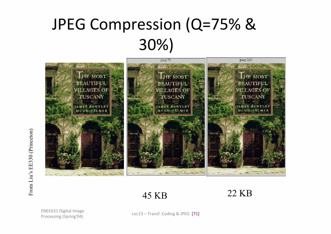
JPEG Compression (Q=75% & 30%)

45 KB 22 KB From

Liu

’s E

E330

(Prin

ceto

n)


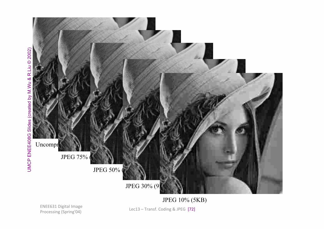
Uncompressed (100KB)

JPEG 75% (18KB)

JPEG 50% (12KB)

JPEG 30% (9KB)

JPEG 10% (5KB)

UM

CP

EN

EE

408G

Slid

es (c

reat

ed b

y M

.Wu

& R

.Liu

© 2

002)

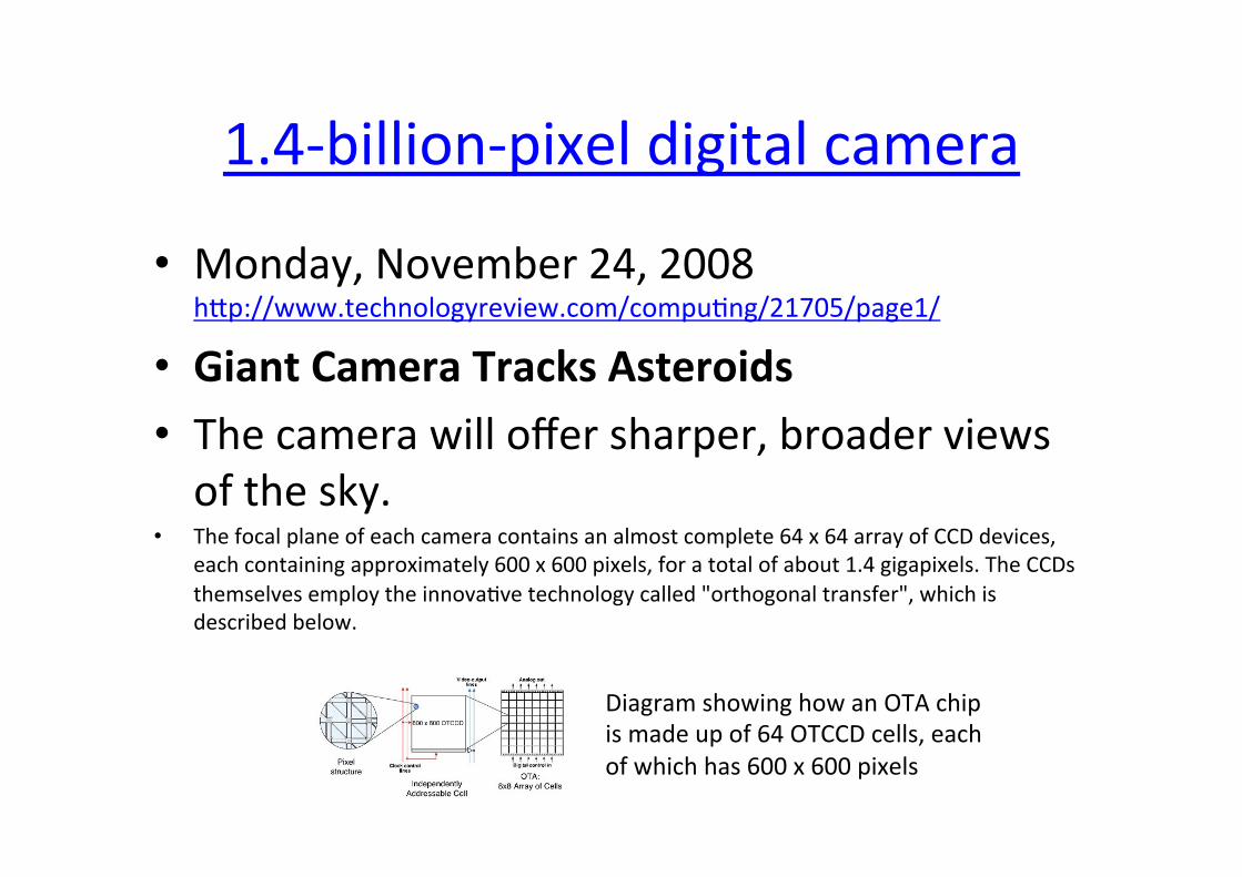
1.4-‐billion-‐pixel digital camera

•  Monday, November 24, 2008 hTp://www.technologyreview.com/compuMng/21705/page1/

•  Giant Camera Tracks Asteroids •  The camera will offer sharper, broader views of the sky.

•  The focal plane of each camera contains an almost complete 64 x 64 array of CCD devices, each containing approximately 600 x 600 pixels, for a total of about 1.4 gigapixels. The CCDs themselves employ the innovaMve technology called "orthogonal transfer", which is described below.

Diagram showing how an OTA chip is made up of 64 OTCCD cells, each of which has 600 x 600 pixels

Fractal compression

•  Fractal Compression group at Waterloo hTp://links.uwaterloo.ca/fractals.home.html

•  A "Hitchhiker's Guide to Fractal Compression" For Beginners �p://links.uwaterloo.ca/pub/Fractals/Papers/Waterloo/vr95.pdf

•  Encode using fractals. •  Search for regions that with a simple transformaMon can be similar to each other.

•  Compressin raMo 20-‐80

•  Moving Pictures Experts Group ( hTp://www.chiariglione.org/mpeg/ )

•  MPEG Compression : hTp://www.cs.cf.ac.uk/Dave/MulMmedia/node255.html •  Screen divided into 256 blocks, where the changes and movements are tracked

•  Only differences from previous frame are shown

•  Compression raMo 50-‐100

•  When one compresses files, can we sMll use fast search techniques without decompressing frst?

•  SomeMmes, yes •  e.g. Udi Manber has developed a method •  Approximate Matching of Run-‐Length Compressed Strings

Veli Mäkinen, Gonzalo Navarro, Esko Ukkonen

•  We focus on the problem of approximate matching of strings that have been compressed using run-‐length encoding. Previous studies have concentrated on the problem of compuMng the longest common subsequence (LCS) between two strings of length m and n , compressed to m' and n' runs. We extend an exisMng algorithm for the LCS to the Levenshtein distance achieving O(m'n+n'm) complexity. Furthermore, we extend this algorithm to a weighted edit distance model, where the weights of the three basic edit operaMons can be chosen arbitrarily. This approach also gives an algorithm for approximate searching of a paTern of m leTers (m' runs) in a text of n leTers (n' runs) in O(mm'n') Mme. Then we propose improvements for a greedy algorithm for the LCS, and conjecture that the improved algorithm has O(m'n') expected case complexity. Experimental results are provided to support the conjecture.

Kolmogorov (or Algorithmic) complexity

•  Kolmogorov, ChaiMn, ... •  What is the compressed version of sequence

'1234567891011121314151617181920212223242526...' ? •  Every symbol appears almost equally frequently, almost

"random" by entropy •  for i=1 to n do print i ; •  Algorithmic complexity (or Kolmogorov complexity) for string

S is the length of the shortest program that reproduces S, o�en noted K(S)

•  CondiMonal complexity : K(S|T). Reproduce S given T. •  hTp://en.wikipedia.org/wiki/Algorithmic_informaMon_theory

•  Algorithmic informaNon theory is a field of study which aTempts to capture the concept of complexity using tools from theoreMcal computer science. The chief idea is to define the complexity (or Kolmogorov complexity) of a string as the length of the shortest program which, when run without any input, outputs that string. Strings that can be produced by short programs are considered to be not very complex. This noMon is surprisingly deep and can be used to state and prove impossibility results akin to Gödel's incompleteness theorem and Turing's halMng problem.

•  The field was developed by Andrey Kolmogorov and Gregory ChaiMn starMng in the late 1960s.

Kolmogorov complexity: size of circle in bits...

Encoder Decoder

Model Model

Data Data

Compressed data

G J ChaiNn

•  hTp://www.cs.umaine.edu/~chaiMn/

•  Distance using K. •  d(S,T) = ( K(S|T) + K(T|S) ) / ( K(S) + K(T) ) •  We cannot calculate K, but we can approximate it

•  E.g. by compression LZ, BWT, etc •  d(S,T) = ( C(ST) + C(TS) ) / ( C(S) + C(T) )

•  Use of Kolmogorov Distance IdenMficaMon of Web Page Authorship, Topic and Domain David Parry (PPT) in OSWIR 2005, 2005 workshop on Open Source Web InformaMon Retrieval

•  Informatsioonikaugus by Mart Sõmermaa, Fall 2003 (in Data Mining Research seminar) hTp://www.egeen.ee/u/vilo/edu/2003-‐04/DM_seminar_2003_II/Raport/P06/main.pdf

TA Lecture 12 Compression.pptx - ut · TextAlgorithms%(6EAP)% % Compression% Jaak%Vilo% 2010%fall%...

Documents

Transcript of TA Lecture 12 Compression.pptx - ut · TextAlgorithms%(6EAP)% % Compression% Jaak%Vilo% 2010%fall%...