T20.1 Chapter Outline Chapter 20 Credit and Inventory Management Chapter Organization 20.1Credit and...
28
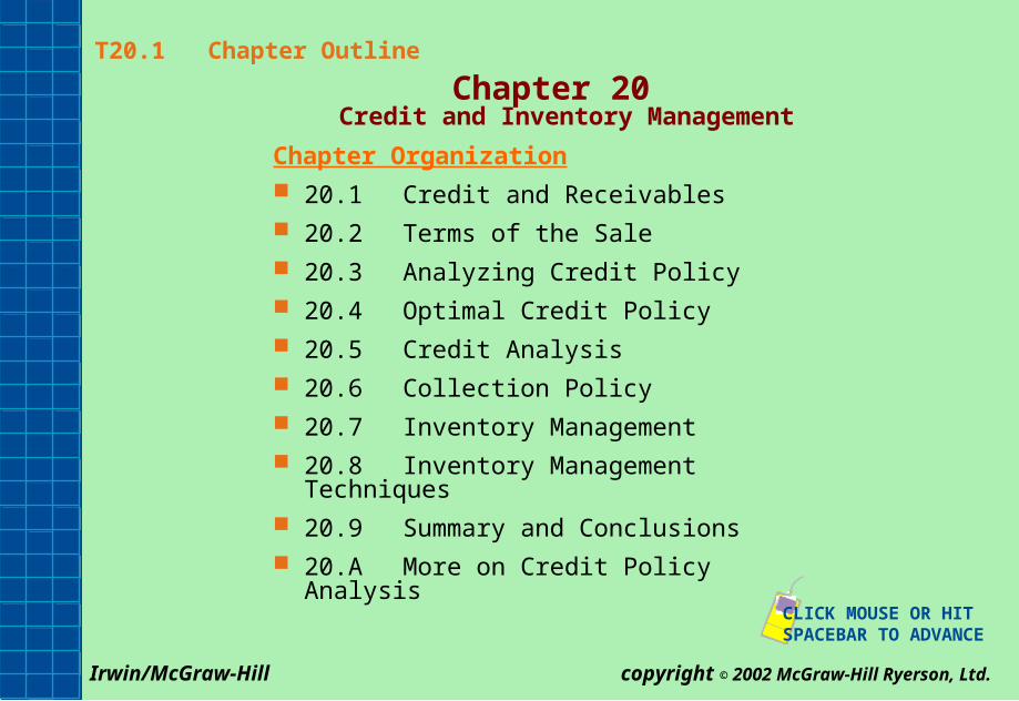
T20.1 Chapter Outline Chapter 20 Credit and Inventory Management Chapter Organization 20.1 Credit and Receivables 20.2 Terms of the Sale 20.3 Analyzing Credit Policy 20.4 Optimal Credit Policy 20.5 Credit Analysis 20.6 Collection Policy 20.7 Inventory Management 20.8 Inventory Management Techniques 20.9 Summary and Conclusions 20.A More on Credit Policy Analysis CLICK MOUSE OR HIT SPACEBAR TO ADVANCE Irwin/McGraw-Hill copyright © 2002 McGraw-Hill Ryerson, Ltd.
-
Upload
cristopher-lanfear -
Category
Documents
-
view
243 -
download
0
Transcript of T20.1 Chapter Outline Chapter 20 Credit and Inventory Management Chapter Organization 20.1Credit and...
T20.1 Chapter Outline
Chapter 20Credit and Inventory Management
Chapter Organization 20.1 Credit and Receivables 20.2 Terms of the Sale 20.3 Analyzing Credit Policy 20.4 Optimal Credit Policy 20.5 Credit Analysis 20.6 Collection Policy 20.7 Inventory Management 20.8 Inventory Management Techniques 20.9 Summary and Conclusions 20.A More on Credit Policy Analysis
CLICK MOUSE OR HIT SPACEBAR TO ADVANCE
Irwin/McGraw-Hill copyright © 2002 McGraw-Hill Ryerson, Ltd.

Irwin/McGraw-Hill copyright © 2002 McGraw-Hill Ryerson, Ltd Slide 2
T20.2 Credit and Inventory Management: Key Issues
Key issues: What is the tradeoff between a flexible versus a restrictive credit
policy? What are the components of an inventory management system?
Preliminaries: credit policy Analysis of a credit policy change Credit information and evaluation of customer credit capacity
Preliminaries: inventory policy Use of EOQ inventory model Extensions of EOQ model Inventory management systems

Irwin/McGraw-Hill copyright © 2002 McGraw-Hill Ryerson, Ltd Slide 3
T20.3 Components of Credit Policy
Terms of sale
The conditions under which a firm sells its goods and services for cash or credit.
Credit analysis
The process of determining the probability that customers will not pay.
Collection policy
Procedures followed by a firm in collecting accounts receivable.

Irwin/McGraw-Hill copyright © 2002 McGraw-Hill Ryerson, Ltd Slide 4
T20.4 The Cash Flows from Granting Credit
Creditsale ismade
Customermailscheck
Firm depositscheck in
bank
Bank creditsfirm’s
account
Cash collection
Accounts receivable
Time
Irwin/McGraw-Hill copyright © 2002 McGraw-Hill Ryerson, Ltd Slide 5
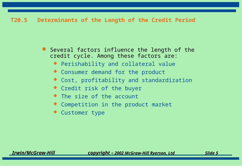
T20.5 Determinants of the Length of the Credit Period
Several factors influence the length of the credit cycle. Among these factors are:
Perishability and collateral value Consumer demand for the product Cost, profitability and standardization Credit risk of the buyer The size of the account Competition in the product market Customer type
Irwin/McGraw-Hill copyright © 2002 McGraw-Hill Ryerson, Ltd Slide 6
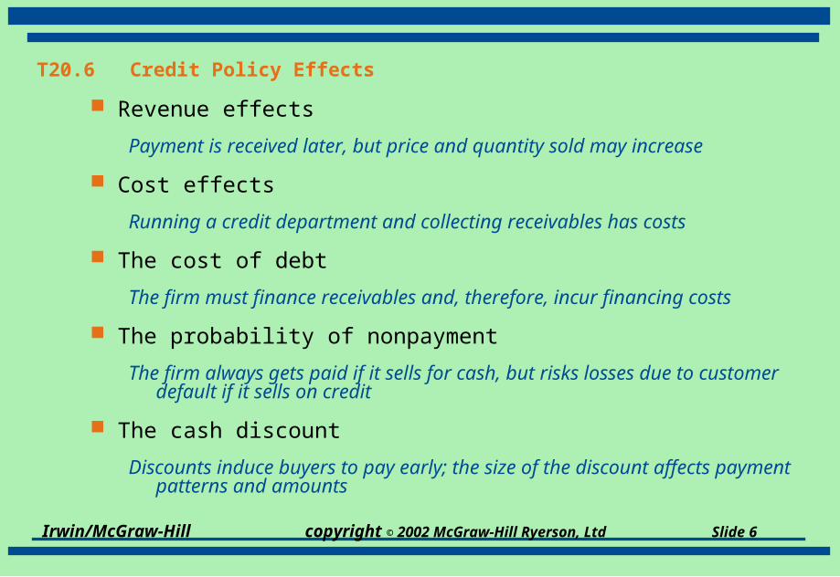
T20.6 Credit Policy Effects
Revenue effects
Payment is received later, but price and quantity sold may increase
Cost effects
Running a credit department and collecting receivables has costs
The cost of debt
The firm must finance receivables and, therefore, incur financing costs
The probability of nonpayment
The firm always gets paid if it sells for cash, but risks losses due to customer default if it sells on credit
The cash discount
Discounts induce buyers to pay early; the size of the discount affects payment patterns and amounts

Irwin/McGraw-Hill copyright © 2002 McGraw-Hill Ryerson, Ltd Slide 7
T20.7 Evaluating a Proposed Credit Policy
P = price per unitv = variable cost per unitQ = current quantity sold per periodQ’ = new quantity expected to be soldR = periodic required return
The benefit of switching is the change in cash flow:
New cash flow - old cash flow
[(P - v) Q’] - [(P - v) Q]
rearranging,
(P - v) (Q’ - Q)
Irwin/McGraw-Hill copyright © 2002 McGraw-Hill Ryerson, Ltd Slide 8
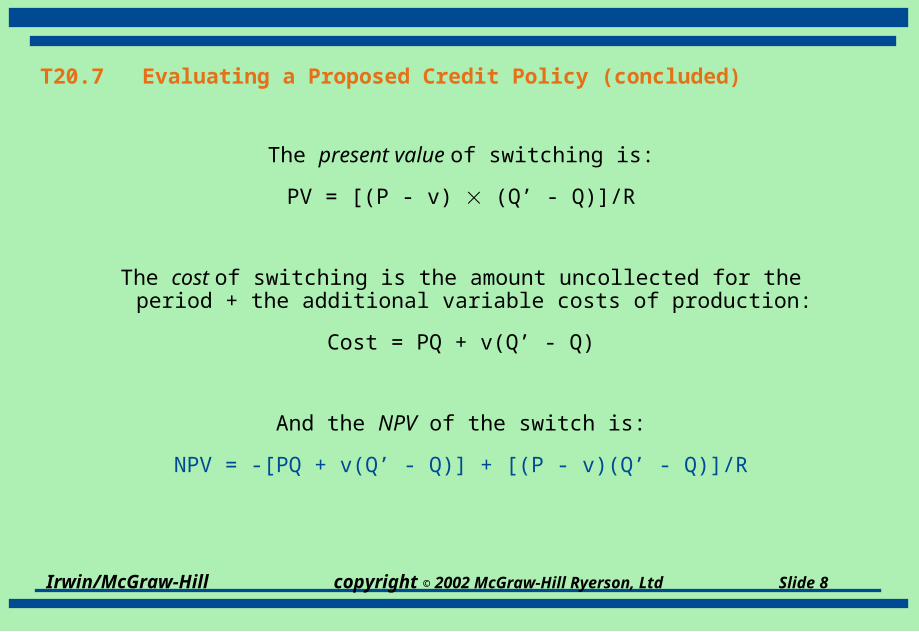
T20.7 Evaluating a Proposed Credit Policy (concluded)
The present value of switching is:
PV = [(P - v) (Q’ - Q)]/R
The cost of switching is the amount uncollected for the period + the additional variable costs of production:
Cost = PQ + v(Q’ - Q)
And the NPV of the switch is:
NPV = -[PQ + v(Q’ - Q)] + [(P - v)(Q’ - Q)]/R

Irwin/McGraw-Hill copyright © 2002 McGraw-Hill Ryerson, Ltd Slide 9
T20.8 The Costs of Granting Credit (Figure 20.1)

Irwin/McGraw-Hill copyright © 2002 McGraw-Hill Ryerson, Ltd Slide 10
T20.9 The Five C’s of Credit
Character
The borrower’s willingness to pay
Capacity
The borrower’s ability to pay
Capital
Financial reserves/borrowing capacity
Collateral
Pledged assets
Conditions
Relevant economic conditions

Irwin/McGraw-Hill copyright © 2002 McGraw-Hill Ryerson, Ltd Slide 11
T20.10 Credit Scoring with Multiple Discriminant Analysis

Irwin/McGraw-Hill copyright © 2002 McGraw-Hill Ryerson, Ltd Slide 12
T20.11 Inventory Management
Inventory Types Raw Materials Work-in-Progress Finished Goods
Inventory Costs Storage and tracking costs Insurance and taxes Losses due to obsolescence, deterioration, or theft Opportunity cost of capital on the invested amount

Irwin/McGraw-Hill copyright © 2002 McGraw-Hill Ryerson, Ltd Slide 13
T20.12 Costs of Holding Inventory (Figure 20.5)

Irwin/McGraw-Hill copyright © 2002 McGraw-Hill Ryerson, Ltd Slide 14
T20.13 Inventory Management Techniques
ABC Approach Compare number of items with the value of the items An illustration of the “80-20” rule
EOQ ModelEconomic Order Quantity is most widely known approach. Inventory depletion rate Carrying costs Shortage costs and Restocking costs Total costs
Extensions to EOQ Safety stocks Reorder points
MRP - Material Requirements Planning
Just-in-Time Inventory

Irwin/McGraw-Hill copyright © 2002 McGraw-Hill Ryerson, Ltd Slide 15
T20.14 ABC Inventory Analysis (Figure 20.4)

Irwin/McGraw-Hill copyright © 2002 McGraw-Hill Ryerson, Ltd Slide 16
T20.15 Inventory Holdings for the Transcan Corporation (Figure 20.6 )
The Transcan Corporation starts with inventory of 3,600 units. The quantity drops to zero by the end of the fourth week. The average inventory is Q/2 = 3,600/2 = 1,800 over the period.

Irwin/McGraw-Hill copyright © 2002 McGraw-Hill Ryerson, Ltd Slide 17
Safety Stocks
T20.16 Safety Stocks and Reorder Points (Figure 20.7)
Inventory
Time
Minimum inventory level
A. Safety Stocks

Irwin/McGraw-Hill copyright © 2002 McGraw-Hill Ryerson, Ltd Slide 18
T20.16 Safety Stocks and Reorder Points (Figure 20.7)
Inventory
Time
Minimum inventory level
B. Reorder points
Delivery time
Delivery time

Irwin/McGraw-Hill copyright © 2002 McGraw-Hill Ryerson, Ltd Slide 19
Safety Stocks
T20.16 Safety Stocks and Reorder Points (Figure 20.7)
Inventory
Time
Minimum inventory level
B. Reorder points
Delivery time
Delivery time

Irwin/McGraw-Hill copyright © 2002 McGraw-Hill Ryerson, Ltd Slide 20
T20.17 Chapter 20 Quick Quiz
1. What is credit analysis?
Estimation of the probability that credit customers will not pay
2. How does one compute the value of the firm’s investment in receivables?
Average daily sales Average collection period (ACP)
3. What is the relationship between credit policy and firm value? How is this quantified?
The optimal credit policy is that which maximizes firm value; the NPV method quantifies the effects of changes in credit policy
4. What is the four-step sequence of procedures to deal with customers whose payments are overdue?
Delinquency letter; telephone call; collection agency; legal action

Irwin/McGraw-Hill copyright © 2002 McGraw-Hill Ryerson, Ltd Slide 21
T20.18 Solution to Problem 20.5
A firm offers terms of 1/7, net 45. What effective annual interest rate (EAR) does the firm earn when a customer does not take the discount? Without doing any calculations, explain what will happen to this effective rate if:
a. the discount is changed to 2 percent.
b. the credit period is increased to 60 days.
c. the discount period is increased to 15 days.
Irwin/McGraw-Hill copyright © 2002 McGraw-Hill Ryerson, Ltd Slide 22
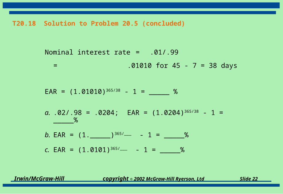
T20.18 Solution to Problem 20.5 (concluded)
Nominal interest rate = .01/.99
= .01010 for 45 - 7 = 38 days
EAR = (1.01010)365/38 - 1 = _____ %
a. .02/.98 = .0204; EAR = (1.0204)365/38 - 1 = _____%
b. EAR = (1._____)365/___ - 1 = _____%
c. EAR = (1.0101)365/___ - 1 = _____%

Irwin/McGraw-Hill copyright © 2002 McGraw-Hill Ryerson, Ltd Slide 23
T20.18 Solution to Problem 20.5 (concluded)
Nominal interest rate = .01/.99
= .01010 for 45 - 7 = 38 days
EAR = (1.01010)365/38 - 1 = 10.13 %
a. .02/.98 = .0204; EAR = (1.0204)365/38 - 1 = 21.42%
b. EAR = (1.0101)365/53 - 1 = 7.17%
c. EAR = (1.0101)365/30 - 1 = 13.01%
Irwin/McGraw-Hill copyright © 2002 McGraw-Hill Ryerson, Ltd Slide 24
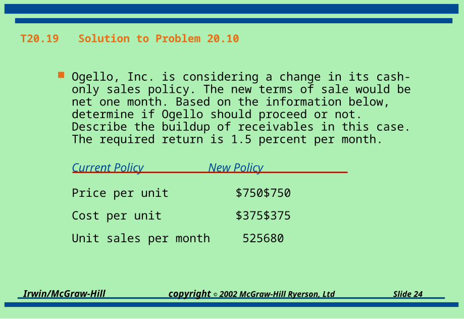
T20.19 Solution to Problem 20.10
Ogello, Inc. is considering a change in its cash-only sales policy. The new terms of sale would be net one month. Based on the information below, determine if Ogello should proceed or not. Describe the buildup of receivables in this case. The required return is 1.5 percent per month.
Current Policy New Policy
Price per unit $750 $750
Cost per unit $375 $375
Unit sales per month 525 680

Irwin/McGraw-Hill copyright © 2002 McGraw-Hill Ryerson, Ltd Slide 25
T20.19 Solution to Problem 20.10 (concluded)
Cost of switching = $___ (525) + $375(_____ - _____) = $_____
Perpetual benefit of switching = ($750 - $375)(680 - 525)= $58,125
NPV = -$_____ + $58,125/_____ = $3,423,125
The firm must bear the cost of sales for one month before they receive any revenue from credit sales, which is why the initial cost is for one month. Receivables will grow over the one month credit period, and then will remain about stable with payments and new sales offsetting one another.

Irwin/McGraw-Hill copyright © 2002 McGraw-Hill Ryerson, Ltd Slide 26
T20.19 Solution to Problem 20.10 (concluded)
Cost of switching = $750(525) + $375(680 - 525) = $451,875
Perpetual benefit of switching = ($750 - $375)(680 - 525)= $58,125
NPV = -$ 451,875 + $58,125/.015 = $3,423,125
The firm must bear the cost of sales for one month before they receive any revenue from credit sales, which is why the initial cost is for one month. Receivables will grow over the one month credit period, and then will remain about stable with payments and new sales offsetting one another.

Irwin/McGraw-Hill copyright © 2002 McGraw-Hill Ryerson, Ltd Slide 27
T20.20 Solution to Problem 20.11
Bell Mfg. uses 1,600 switch assemblies per week and then reorders another 1,600. If the relevant carrying cost per assembly is $40, and the fixed order cost is $800, is Bell’s inventory policy optimal? Why or why not?
Carrying costs = (_____/2)($40) = $_____
Order costs = (52)($_____) = $_____
EOQ = [2(52)(1,600)($800)/$40]1/2 = _____ units
The firm’s policy (is/is not) optimal, since the costs are not equal.
Bell should _______ the order size and _______ the number of orders per year.

Irwin/McGraw-Hill copyright © 2002 McGraw-Hill Ryerson, Ltd Slide 28
T20.20 Solution to Problem 20.11
Bell Mfg. uses 1,600 switch assemblies per week and then reorders another 1,600. If the relevant carrying cost per assembly is $40, and the fixed order cost is $800, is Bell’s inventory policy optimal? Why or why not?
Carrying costs = (1,600/2)($40) = $32,000
Order costs = (52)($800) = $41,600
EOQ = [2(52)(1,600)($800)/$40]1/2 = 1,825 units
The firm’s policy is not optimal, since the costs are not equal.
Bell should increase the order size and decrease the number of orders per year.