![MODELAGEM E AVALIAÇÃO DE DESEMPENHO · #Call the finish procedure after 5 seconds of simulation time $ns at 5.0 "finish" #Run the ... [open out.tr w] $ns trace-all $tf #Simulation](https://static.fdocuments.in/doc/165x107/5d16734d88c99309378bee70/modelagem-e-avaliacao-de-call-the-finish-procedure-after-5-seconds-of-simulation.jpg)
T-SIMn: A trace collection and simulation framework for ...
17
Computer Communications 117 (2018) 116–132 Contents lists available at ScienceDirect Computer Communications journal homepage: www.elsevier.com/locate/comcom T-SIMn: A trace collection and simulation framework for 802.11n networks Ali Abedi ∗ , Tim Brecht, Andrew Heard David R. Cheriton School of Computer Science, University of Waterloo, Canada a r t i c l e i n f o Article history: Available online 17 August 2017 Keywords: Trace-based simulation Performance evaluation 802.11 WiFi Trace collection a b s t r a c t In this paper, we describe the design, implementation and evaluation of a new framework for the trace- based evaluation of 802.11n networks, which we call T-SIMn. In order to accurately estimate the fate of frames that could have been sent at any rate, traces collected for use in trace-based simulators, like T-SIMn, require a sufficiently large number of samples to be collected using each different rate in a rel- atively short period of time. In this paper, we devise two novel techniques for collecting and processing traces for 802.11n networks that incorporate Frame Aggregation (FA). The first technique, called direct measurement, samples all rates while aggregating the maximum number of possible frames for each sample. This approach is attractive because frame error rates (FERs) may vary with the position of the frame within the aggregated frame and this techniques directly captures the fate of each subframe. How- ever, the length of the aggregated frames limits this approach to smaller numbers of rates, making it unusable for devices with 3 antennas (e.g., 96 rates). As a result, we also devise second technique that collects traces with frame aggregation turned off, permitting a larger number of rates to be sampled within the same period of time. This approach, called inferred measurement, infers the FER of each sub- frame using models derived from calibration traces combined with a new measure of changing channel conditions we call the channel dynamic indicator (CDI). Using the direct measurement methodology, we evaluate the T-SIMn framework by collecting traces using an iPhone, which is representative of a wide variety of one antenna devices. We show that our framework can be used to accurately simulate sev- eral scenarios and demonstrate the fidelity of SIMn by uncovering problems with our initial evaluation methodology. We then demonstrate that our inferred measurement technique permits us to collect traces that sample all 96 rates in a 3x3:3 802.11n MIMO systems. These traces are then used to accurately sim- ulate transmissions in environments with highly variable channel conditions that include mobility and multiple sources of interference. We expect that the T-SIMn framework will be suitable for easily and fairly comparing algorithms that must be optimized for different and varying 802.11n channel conditions, which are challenging to evalu- ate experimentally. These include rate adaptation, frame aggregation and channel bandwidth adaptation algorithms. Crown Copyright © 2017 Published by Elsevier B.V. All rights reserved. 1. Introduction With billions of WiFi devices now in use, combined with the rising popularity of high-bandwidth applications such as stream- ing video, demands on WiFi networks continue to rise. The 802.11n standard introduced several new physical layer features including MIMO, 40 MHz channels, denser modulations, and a shorter guard interval, to increase throughput. We refer to the combination of features as a rate configuration. Combinations of these features re- ∗ Corresponding author. E-mail addresses: [email protected], [email protected] (A. Abedi), [email protected] (T. Brecht), [email protected] (A. Heard). sults in up to 128 different rate configurations. In order to opti- mize throughput in an 802.11n network, we must choose the rate configuration that results in the best trade-off between physical layer transmission rates and error rates, which is highly depen- dent on environmental conditions. Because the radio spectrums are shared by WiFi devices included in computers, cell phones and tablets; as well as Bluetooth devices, wireless keyboards/mice, cordless phones, and microwave ovens, it is challenging to experi- mentally evaluate and compare the performance of WiFi networks. Therefore, we need new techniques for understanding and evalu- ating how to best use 802.11n features. Previously, we proposed a solution [1] that uses traces to cap- ture environmental conditions, rather than models, to simulate http://dx.doi.org/10.1016/j.comcom.2017.08.008 0140-3664/Crown Copyright © 2017 Published by Elsevier B.V. All rights reserved.
Transcript of T-SIMn: A trace collection and simulation framework for ...

Computer Communications 117 (2018) 116–132
Contents lists available at ScienceDirect
Computer Communications
journal homepage: www.elsevier.com/locate/comcom
T-SIMn: A trace collection and simulation framework for 802.11n
networks
Ali Abedi ∗, Tim Brecht, Andrew Heard
David R. Cheriton School of Computer Science, University of Waterloo, Canada
a r t i c l e i n f o
Article history:
Available online 17 August 2017
Keywords:
Trace-based simulation
Performance evaluation
802.11
WiFi
Trace collection
a b s t r a c t
In this paper, we describe the design, implementation and evaluation of a new framework for the trace-
based evaluation of 802.11n networks, which we call T-SIMn. In order to accurately estimate the fate
of frames that could have been sent at any rate, traces collected for use in trace-based simulators, like
T-SIMn, require a sufficiently large number of samples to be collected using each different rate in a rel-
atively short period of time. In this paper, we devise two novel techniques for collecting and processing
traces for 802.11n networks that incorporate Frame Aggregation (FA). The first technique, called direct
measurement, samples all rates while aggregating the maximum number of possible frames for each
sample. This approach is attractive because frame error rates (FERs) may vary with the position of the
frame within the aggregated frame and this techniques directly captures the fate of each subframe. How-
ever, the length of the aggregated frames limits this approach to smaller numbers of rates, making it
unusable for devices with 3 antennas (e.g., 96 rates). As a result, we also devise second technique that
collects traces with frame aggregation turned off, permitting a larger number of rates to be sampled
within the same period of time. This approach, called inferred measurement, infers the FER of each sub-
frame using models derived from calibration traces combined with a new measure of changing channel
conditions we call the channel dynamic indicator (CDI). Using the direct measurement methodology, we
evaluate the T-SIMn framework by collecting traces using an iPhone, which is representative of a wide
variety of one antenna devices. We show that our framework can be used to accurately simulate sev-
eral scenarios and demonstrate the fidelity of SIMn by uncovering problems with our initial evaluation
methodology. We then demonstrate that our inferred measurement technique permits us to collect traces
that sample all 96 rates in a 3x3:3 802.11n MIMO systems. These traces are then used to accurately sim-
ulate transmissions in environments with highly variable channel conditions that include mobility and
multiple sources of interference.
We expect that the T-SIMn framework will be suitable for easily and fairly comparing algorithms that
must be optimized for different and varying 802.11n channel conditions, which are challenging to evalu-
ate experimentally. These include rate adaptation, frame aggregation and channel bandwidth adaptation
algorithms.
Crown Copyright © 2017 Published by Elsevier B.V. All rights reserved.
s
m
c
l
d
a
a
c
m
1. Introduction
With billions of WiFi devices now in use, combined with the
rising popularity of high-bandwidth applications such as stream-
ing video, demands on WiFi networks continue to rise. The 802.11n
standard introduced several new physical layer features including
MIMO, 40 MHz channels, denser modulations, and a shorter guard
interval, to increase throughput. We refer to the combination of
features as a rate configuration . Combinations of these features re-
∗ Corresponding author.
E-mail addresses: [email protected] , [email protected] (A. Abedi),
[email protected] (T. Brecht), [email protected] (A. Heard).
T
a
t
http://dx.doi.org/10.1016/j.comcom.2017.08.008
0140-3664/Crown Copyright © 2017 Published by Elsevier B.V. All rights reserved.
ults in up to 128 different rate configurations. In order to opti-
ize throughput in an 802.11n network, we must choose the rate
onfiguration that results in the best trade-off between physical
ayer transmission rates and error rates, which is highly depen-
ent on environmental conditions. Because the radio spectrums
re shared by WiFi devices included in computers, cell phones
nd tablets; as well as Bluetooth devices, wireless keyboards/mice,
ordless phones, and microwave ovens, it is challenging to experi-
entally evaluate and compare the performance of WiFi networks.
herefore, we need new techniques for understanding and evalu-
ting how to best use 802.11n features.
Previously, we proposed a solution [1] that uses traces to cap-
ure environmental conditions, rather than models, to simulate

A. Abedi et al. / Computer Communications 117 (2018) 116–132 117
Fig. 1. FA: Maximum theoretical throughput.
8
i
H
c
8
q
b
p
o
t
w
t
f
a
e
i
l
t
l
t
s
r
a
t
t
a
m
Fig. 2. Rate notation.
d
o
o
d
t
w
i
i
o
I
m
d
w
s
2
2
t
d
r
b
n
c
u
t
s
n
T
t
e
s
i
t
2
t
T
g
S
d
p
p
p
02.11g networks with high fidelity. We expected that extend-
ng this solution to 802.11n networks would be relatively simple.
owever, it turned out that this is actually a very interesting and
hallenging problem, due to MAC layer frame aggregation (FA) in
02.11n. The complications introduced by frame aggregation re-
uired a complete redesign of major components of our trace-
ased simulator. While the faster transmission rates are an im-
ortant factor in the throughput gains afforded by 802.11n, it is
nly when they are used in combination with frame aggregation
hat 802.11n networks achieve significant increases in throughput
hen compared with 802.11g. Frame Aggregation (FA) allows mul-
iple MAC layer frames to be combined into a large physical layer
rame so that they can be transmitted and acknowledged as one
ggregated frame, which results in the channel being used more
fficiently.
To demonstrate the importance of FA, Fig. 1 shows the max-
mum theoretical throughput obtained using the highest physical
ayer transmission rate in 802.11n for one, two and three spa-
ial streams, respectively. Without frame aggregation throughput is
imited to about 50 Mbps. However, when aggregating 32 frames,
hroughput increases to 350 Mbps.
Because performance is so heavily dependent on FA, accurate
imulation of FA is crucial for T-SIMn to be useful in the study of a
ange of active research topics. This includes the evaluation of: link
daptation algorithms [2] (which studies physical layer configura-
ions such as rate adaptation [3,4] and channel bandwidth adapta-
ion [5,6] ) and frame aggregation algorithms [7,8] . We refer to link
daptation and frame aggregation algorithms collectively as opti-
ization algorithms .
The contributions of this paper are:
• We design, implement and evaluate a trace-based simulation
framework (T-SIMn) for realistic and repeatable performance
evaluations of 802.11n networks.
• We design and evaluate a trace collection methodology (called
direct measurement ), which is simple and easy to use but suit-
able only for devices with a smaller number of transmission
rates (e.g., the vast majority of cellphones and tablets that have
only one antenna). Using an iPhone as the receiving device we
show that collecting traces using direct measurement combined
with our prototype implementation of T-SIMn produce highly
accurate simulation results.
• We design and evaluate a trace collection methodology (called
indirect measurement ), which is more complex to use but is
suitable for devices with many more transmission rates (e.g.,
some desktop systems with three antennas supporting 96
rates). We demonstrate that indirect measurement can be com-
bined with T-SIMn to obtain highly accurate simulations of a
device with 96 rates.
• While designing the indirect measurement methodology we de-
veloped a new technique for estimating the frame error rate of
subframes within an aggregated frame that takes into account
channel dynamics. We first show that changes in the Received
Signal Strength Indicator (RSSI) of ACKs can be used to infer the
channel dynamics which in conjunction with the delivery ratio
of the first MAC Protocol DATA Unit (MPDU) can be used to ac-
curately estimate the fate of other subframes in an aggregated
MPDU (A-MPDU). We then develop a model that can be used
with the T-SIMn simulator and demonstrate that the model is
accurate.
The paper begins by providing some necessary background and
escribing related work in Section 2 . We then present an overview
f the T-SIMn framework in Section 3 , followed by a description
f the test bed used in this study (in Section 4 ). In Section 5 , we
escribe the components of the T-SIMn framework and evaluate
he accuracy of these components. We then evaluate the frame-
ork as a whole in Section 6 , by utilizing traces collected using an
Phone and the direct measurement methodology. In Section 7 , we
nvestigate the limitations of the direct measurement methodol-
gy when used with devices that support many transmission rates.
n Section 8 , we propose and evaluate the inferred measurement
ethodology which is designed to be used in situations where the
irect trace collection technique is unable to sample enough rates
ithin the required period of time. Finally, conclusions are pre-
ented in Section 9 .
. Background and related work
.1. Rate configurations
In 802.11g, a transmission rate can be uniquely identified by
he index of the Modulation and Coding Scheme (MCS). This in-
ex alone is no longer sufficient to uniquely identify an 802.11n
ate, as the transmission rate is now also dependent on the num-
er of Spatial Streams (SSs), the Guard Interval (GI) and the Chan-
el Bandwidth (CB). We refer to this set of parameters as a rate
onfiguration. In the interest of brevity, Fig. 2 introduces notation
sed for describing a rate configuration (sometimes simply referred
o as a rate).
The first two characters represent the number of spatial
treams (in the example 2S stands for two spatial streams). The
ext two characters represent the MCS index (I6 means index 6).
his is followed by information about whether a Long Guard In-
erval (LGI) or Short Guard Interval (SGI) are being used (in the
xample LG means and LGI is used). The next three characters de-
cribe whether the channel bandwidth is 20 or 40 MHz (20 MHz
n the example). Finally the number after the equal sign indicates
he resulting physical rate (104 Mbps in the example).
.2. 802.11N frame aggregation
Frame aggregation (FA) is a new MAC layer feature in 802.11n
hat allows multiple frames to be combined to form a larger frame.
he 802.11n standard defines two types of frame aggregation: Ag-
regated MAC Protocol DATA Unit (A-MPDU) and Aggregated MAC
ervice DATA Unit (A-MSDU) . These two types of frame aggregation
iffer by where in the protocol stack aggregation is done. In this
aper, we use A-MPDU frame aggregation as it is more widely sup-
orted by WiFi devices, including the Atheros devices used in this
aper.

118 A. Abedi et al. / Computer Communications 117 (2018) 116–132
l
p
A
R
c
n
u
t
i
w
t
a
f
3
a
a
t
8
a
i
a
s
t
l
c
a
t
r
8
t
c
s
d
c
d
r
t
(
A
t
t
c
p
f
t
3
c
c
f
u
c
c
w
i
By sending multiple MPDUs 1 as an A-MPDU, the sender only
performs channel sensing, backoff, Distributed Inter-Frame Space
(DIFS), Short Inter-Frame Space (SIFS) and wait for an ACK once
for the entire set of MPDUs. This results in a greater proportion
of time being spent transmitting data, increasing the air time ef-
ficiency. The receiver sends back a Block ACK which acknowledges
all MPDUs at once. In this work, we use MPDU and subframe in-
terchangeably.
2.3. Related work
Conducting experiments is a common technique for evaluating
the performance of WiFi networks. The advantage of this approach
is that real-world wireless channel conditions are captured. How-
ever, it is challenging to conduct repeatable experiments [9] be-
cause channel conditions can vary significantly between trials due
to many factors, including mobility, changes in the environment
(including the movement of people who are nearby), and the pres-
ence of WiFi and non-WiFi interferers [10] .
Simulation is a common technique for evaluating the perfor-
mance of 802.11 networks. Since both the physical and MAC layers
are simulated in this approach, comparisons are repeatable. Popu-
lar 802.11 network simulators include ns-3 [11] , OMNeT ++ [12] ,
OPNET Modeler [13] (renamed, Riverbed Modeler) and Qual-
Net [14] . Unfortunately, these simulators may not reflect real-world
performance due to the challenging nature of simulating wire-
less signals in the physical environment. WiFi signals are impacted
by many factors, including the distance between devices, material
types of surrounding objects and walls, wavelength, mobility and
many more [15] . These simulators utilize models for signal prop-
agation, error rates and interference and each model must trade-
off computational complexity and accuracy [15] . Additionally, the
complexity and time varying nature of all of the factors that can
affect a frame’s fate makes it incredibly challenging to obtain accu-
rate results, especially since models of one environment (e.g., one
home) may not necessarily work in another environment (e.g., an
office or even a different home). In the case of environments with
mobility, this model may change over time. As a result existing
simulators suffer from practical limitations For instance, OMNeT ++does not support multi-path signal propagation [16] , which is an
important prerequisite for simulating MIMO transmissions. There
is also no support for MIMO in ns-3. Rather than simulating the
physical layer, we collect traces to capture the impact of the phys-
ical layer on frame fates, allowing us to handle more complex sce-
narios than can be accurately modeled by traditional simulators.
Emulation is another alternative for evaluating and studying
802.11 networks. The most common approach is to use real WiFi
devices connected by wire to a Field- Programmable Gate Array
(FPGA) that simulates signal propagation [17] . An emulation test
bed by Judd and Steenkiste [18] is one of the most prominent ex-
amples of this type of system. As real devices are used, the MAC
and parts of the physical layer are not simulated. However, signal
propagation is simulated using the FPGA to alter the signals being
transmitted between devices. The major disadvantage of this ap-
proach is that realism is again limited by the models used to sim-
ulate the physical layer.
To increase the realism of emulators, hybrid approaches using
traces to simulate the physical layer and emulation for the MAC
layer have also been proposed [18,19] , however these have been
limited to 802.11b networks and rely on measurements of Signal-
to-Noise Ratio (SNR) to simulate the physical layer. However, the
SNR can not be used to accurately predict frame fates [20] . Instead,
we rely on traces to directly capture the impact of the physical
1 MAC header + MAC payload (IP packet).
n
t
ayer on frame fates and simulate the well-defined MAC layer. This
rovides an excellent combination of repeatability and fidelity.
T-RATE [1] is our trace-driven framework for evaluating Rate
daptation Algorithms (RAAs) designed for 802.11g networks. T-
ATE eschews the modeling and emulation of wireless channel
onditions in favor of traces that capture channel access and chan-
el error rate information. These traces are used to simulate RAAs
sing channel conditions limited only by the environment in which
races are collected. Despite the high fidelity of T-RATE, it is lim-
ted to the evaluation of RAAs in 802.11g networks. In this paper,
e design and evaluate T-SIMn, a more general framework for the
race-based evaluation of 802.11n networks. The most prominent
nd challenging contribution in T-SIMn is the accurate handling of
rame aggregation.
. The T-SIMn framework
The main goal of T-SIMn is to achieve repeatability and re-
lism when evaluating the performance of 802.11n networks. To
chieve this goal, T-SIMn records all channel conditions that affect
hroughput in a trace and then uses this trace to simulate different
02.11n optimization algorithms such as link adaptation and frame
ggregation. As a result, T-SIM can be used to achieve repeatabil-
ty by using an identical trace to evaluate different algorithms. In
ddition, it achieves realism since T-SIMn relies on traces that are
ubject to and include information related to actual channel condi-
ions rather than using wireless channel models , which are known to
ack realism [21,22] .
To simulate 802.11n networks with high fidelity, we need to ac-
urately compute the transmission time of a frame and consider
ll factors that can affect throughput. Computing the transmission
ime for a frame is a relatively easy task and is done very accu-
ately in our simulator by using timing information available in the
02.11n standard ( Section 5.2 provides more details). Environmen-
al factors may affect 802.11 channel access (i.e., CSMA/CA) and
hannel error rate. If a WiFi or non-WiFi device operating at the
ame frequency is active during channel sensing, it forces a sender
evice to back off and therefore limits the number of frames that
an be sent. If WiFi or non-WiFi devices interfere with the receiver
evice, the channel error rate may increase. In T-SIMn, to accu-
ately simulate the time required for frame transmission we need
o determine: the delay (overhead) imposed by channel sensing
i.e., CSMA/CA), how long it takes to transmit a frame (including
CK reception and DCF mandatory wait times), and whether or not
he transmitted frame is received correctly.
T-SIMn uses two phases to simulate 802.11n. The first phase is
race collection, where a log containing the data necessary for ac-
urately simulating an 802.11n experiment is collected. The second
hase is simulation, where the trace is used to determine frame
ates, transmission delays and throughput. We now explain these
wo phases.
.1. Trace collection
The purpose of trace collection is to capture channel access and
hannel error rate information (i.e., a trace), for each 802.11n rate
onfiguration. To enable the simulation of any link adaptation and
rame aggregation algorithm at time t , T-SIMn must be able to sim-
late the transmission of an A-MPDU of any length sent with any
hosen rate configuration. This requirement makes trace collection
hallenging, since at time t , only one particular rate configuration
ith a specific A-MPDU length can be transmitted. Therefore, no
nformation is available at that time concerning the other combi-
ations of rate configuration and frame lengths.
To address this problem we have designed two trace collec-
ion techniques that sample all rate configurations in a round

A. Abedi et al. / Computer Communications 117 (2018) 116–132 119
r
f
m
a
w
w
o
c
s
s
d
c
t
c
n
I
c
u
t
c
w
i
t
i
D
f
c
M
t
d
t
t
l
n
w
b
t
t
c
p
s
a
w
c
f
b
(
i
W
m
f
f
W
A
i
t
t
3
o
w
w
m
t
c
o
a
a
s
d
fi
(
i
n
w
w
t
c
a
m
t
n
b
h
m
s
2
b
b
t
e
p
s
t
r
3
f
r
a
t
o
b
i
obin fashion. The direct measurement methodology is suitable
or studies using devices that support a limited number of trans-
ission rates such as one antenna devices (e.g., many cellphones
nd tablets). We believe that the direct measurement will be used
hen possible due to its simplicity. However, for 802.11n devices
ith a larger number of transmission rates, we design a method-
logy called inferred measurement. We now explain the common
haracteristics of both methods and the details of the direct mea-
urement methodology. A detailed description of the inferred mea-
urement methodology is presented in Section 8 .
With both trace collection techniques, we modify the device
river so that the rate adaptation algorithm, instead of trying to
hoose the best rate, cycles through all of the rates supported by
he device in a round-robin fashion for the duration of the trace
ollection. After a frame is transmitted, the sender switches to the
ext rate; wrapping back around after all rates have been sampled.
f we sample all rate configurations within the time a channel is
onsidered stationary (i.e., the channel coherence time), all config-
rations experience the same channel conditions. During simula-
ion, to obtain the error rate of a rate configuration at time t , we
ompute an average error rate for that configuration over a time
indow centered at t .
If the error rates of the MPDUs within an aggregated frame are
dentical, we could disable frame aggregation during trace collec-
ion and simulate aggregated frames of any size, by simply apply-
ng the error rate of (non-aggregated) collected frames to all MP-
Us in an A-MPDU. However, a recent study [7] shows that the
rame error rate of the MPDUs within an A-MPDU are not identi-
al . More specifically, they show that the frame error rate of early
PDUs (i.e., closer to the physical header) are lower than MPDUs
hat appear latter in the A-MPDU. Although we confirm that in-
ividual MPDUs have different error rates, we find patterns other
han the increasing error rate pattern (observed in [7] ). We discuss
hese findings in greater detail in Section 5.4.1 . Note that this prob-
em was not an issue in our 802.11g framework since 802.11g does
ot support frame aggregation. One might imagine that a solution
ould be, during trace collection, to attempt to sample all com-
inations of A-MPDUs from length 1 (i.e., no frame aggregation)
o the maximum number of MPDUs allowed in an A-MPDU. Since
his procedure would be required for all rate configurations, it be-
omes impossible to sample all combinations in a sufficiently short
eriod of time (i.e., within the channel coherence window). As a re-
ult, the direct measurement methodology infers the fate of MPDUs in
n A-MPDU from a longer A-MPDU. Therefore, during trace collection,
e only need to sample the longest possible A-MPDU for each rate
onfiguration and infer the FERs of any shorter A-MPDU for that rate
rom the longer A-MPDU.
In both methodologies, in order to record the delay imposed
y channel access (CSMA/CA), we use Cycle Counter Information
CCI) reported by a modified ath9k driver as explained in detail
n Section 5.3 . These counters help us infer the delay caused by
iFi and non-WiFi devices when performing channel sensing. We
odify the ath9k driver to print a log entry after each aggregated
rame (A-MPDU) transmission has completed, which includes the
ate of each MPDU and the CCI. It may be possible to use other
iFi devices for trace collection. However, we chose the Atheros
R9380 chipset because of the availability of the source code and
ts support for CCI. Our trace collection requires the modification of
he rate adaptation algorithm and, as will be required in Section 7 ,
he frame aggregation algorithm.
.2. Simulation
The trace processing phase uses a trace to simulate different
ptimization algorithms. The simulator component of our frame-
ork (called SIMn) performs a time based simulation using a trace,
here the sender saturates the link to the receiver by sending as
any aggregated frames as possible.
Figs. 3 illustrates the work flow of SIMn. Solid lines represent
he execution flow of the simulator, with the direction being indi-
ated by a closed (i.e., filled) arrow. Dashed lines indicate the flow
f data, with the recipient of the data being indicated with an open
rrow. As depicted in Fig. 3 , a simulation in SIMn proceeds using
n event loop, starting at time t = 0 , that performs the following
teps:
1. Check the collected trace for unprocessed WiFi delays that oc-
curred before time t . If WiFi delays exist, t is incremented by
the duration of the delay. This is repeated until all WiFi delays
that have occurred before t have been processed.
2. Determine any non-WiFi delays that occur at time t and incre-
ment t by the duration of the delay.
3. If there are fewer than two aggregate frames (one in transmis-
sion and one queued), create an aggregate frame and add it to
the queue.
4. Compute the time to transmit the A-MPDU.
5. Determine the fate of each subframe i in the aggregate frame
using the Subframe Index Error Rate (SFIER) at time t , rate r and
index i . SFIERs are discussed in detail in Section 5.4.1 . Failed
subframes are rescheduled for retransmission if the retry limit
has not been exceeded.
This process repeats until the simulation time is equal to the
uration of the collected trace. To create an aggregated frame we
rst compute the maximum allowed size of the aggregated frame
detailed in Section 5.2.2 ). Then MPDUs are added to an A-MPDU
n a loop until the maximum size is reached. The MPDUs are either
ew frames arriving from an application or failed MPDUs that are
aiting for retransmission. Rescheduled frames are given priority
hen forming aggregate frames.
To determine the fate of a subframe with index i that needs
o be sent at simulated time t with rate configuration r , T-SIMn
onsiders all samples for the rate r and subframe index i in the
veraging window (t − window_size/2) ms to (t + window_size/2)
s, from the collected trace. The averaging window should be less
han the channel coherence time for the environment so that chan-
el conditions are relatively constant with respect to the frames
eing used to determine the fate of frames at time t . Channel co-
erence time depends on many factors (e.g., the speed of move-
ent and channel frequency). In indoor environments at walking
peeds channel coherence time is reported to be approximately
00 ms for the 2.4 GHz band [23] and 100 ms for the 5 GHz
and [24] . Because all experiments in this paper use the 5 GHz
and, we use an averaging window of 200 ms (i.e., t − 100 ms to
+ 100 ms), which corresponds to a 100 ms coherence time. Our
valuation in Section 6 shows that an averaging window of 200 ms
roduces accurate results in our mobile environment at walking
peeds, when performing round-robin trace collection with 1 an-
enna. However, this parameter can be easily tailored to the envi-
onment.
.3. Frame aggregation notation
To concisely describe limits on the length of an aggregated
rame (i.e., the number of subframes) for a particular rate configu-
ation, we introduce the notation:
FA (SIM | COL)
= maximum number of aggregated subframes
For example, FA SIM = 16 means that the simulator is allowed to
ggregate a maximum of 16 subframes (we omit rate configura-
ion information; it is not needed for our purposes). The number
f subframes in a specific aggregated frame may be further limited
y the Block-Ack window discussed in detail in Section 5.2.2 . Sim-
larly, FA COL = 32 means that the driver was limited to aggregat-

120 A. Abedi et al. / Computer Communications 117 (2018) 116–132
Fig. 3. T-SIMn simulation flowchart.
Fig. 4. Floor plan of the test bed environment.
t
T
B
t
t
b
ing a maximum of 32 subframes during trace collection . We use the
notation FA SIM = MAX and FA COL = MAX to mean that we impose no
restrictions, beyond those in the 802.11n standard and the ath9k
driver (i.e., 32 MPDUs), on the aggregated frame length during
simulation and trace collection, respectively. Lastly, FA SIM = FA COL means the limits on the aggregated frame are the same during
simulation and trace collection.
4. Test bed
Our test bed is located in cubicles in a large room, as well as
some separate offices on a university campus. Fig. 4 shows the
floor plan for the cubicles and offices. Four cubicles are located
in the area near the labels (AP) and (C) and four are located be-
tween the two grey bars (which indicate paneled dividers between
the two sets of cubicles). The five smaller rooms are two person
offices and the larger room at the top right is a meeting room.
Our WiFidevices include two desktop computers housing identical
TP-Link TL-WDN4800 PCIe cards, an Apple MacBook Pro-(Retina,
15-inch, Mid 2012), an Apple iPhone 6, and a laptop configured
o use a TP-Link TL-WDN4200 dual-band wireless N USB adapter.
he TP-Link cards use an Atheros AR9380 chipset, while the Mac-
ook and iPhone use Broadcom BCM4331 and BCM4339, respec-
ively. The USB adapter contains an Ralink RT3573 chipset and uses
he rt2800usb (Ralink) device driver. Although all devices are dual-
and (2.4 and 5 GHz), several experiments are conducted using the

A. Abedi et al. / Computer Communications 117 (2018) 116–132 121
5
d
t
(
p
9
u
u
a
t
t
t
I
d
I
c
a
s
U
s
i
t
f
a
t
t
m
X
e
t
5
5
a
m
c
(
t
r
l
d
p
a
I
m
i
c
l
e
w
c
w
t
c
h
u
p
v
f
Fig. 5. Fidelity of PHY layer features simulation.
5
t
r
a
s
s
5
t
(
m
h
c
u
q
w
t
c
i
r
2
t
G
a
C
h
W
p
a
m
s
r
t
S
i
c
t
N
t
t
5
s
(
GHz band because the Apple devices used in these experiments
o not support 40 MHz channel bandwidths in the 2.4 GHz spec-
rum. Except for the iPhone 6, which contains only one antenna
i.e., 32 transmission rates), all devices contain three antennas sup-
orting three spatial streams in a 3x3:3 MIMO configuration with
6 transmission rates.
We create an 802.11n Access Point (AP), shown as (AP) in Fig. 4 ,
sing hostapd and collect traces while that system sends frames
sing our modified ath9k driver. Although the AP could be used
s the sender or the receiver , we use the computer designated as
he AP as the sender in all experiments. The major advantage of
his approach is that there are fewer requirements imposed on
he receiver , which does not need to be capable of creating an AP.
n addition, the receiver does not need to use a modified ath9k
river and, as a result, can be any 802.11n-capable device that runs
perf3; this includes a wide variety of devices, even an iPhone. We
reate a network between the AP ( sender ) and a client, which acts
s a receiver. To collect a trace the sender saturates the link by
ending as many 1,470 byte UDP frames as possible using Iperf3.
nless otherwise noted, we aggregate the maximum number of
ubframes (i.e., FA COL = MAX ). We use the second desktop as a receiver , shown as © in Fig. 4 ,
n the stationary experiments. It is located less than 1 meter from
he AP with line of sight so we can collect error-free traces needed
or some experiments. The MacBook, iPhone, and the USB adapter
re used for mobile experiments. When it is necessary to minimize
he amount of uncontrolled WiFi interference, we use channels in
he 5 GHz band that are unused by other APs in the vicinity. We
onitor all channels for interference using an AirMagnet Spectrum
T spectrum analyzer. For generating controlled non-WiFi interfer-
nce we use an RF Explorer Handheld Signal Generator (RFE6GEN)
hat we control programmatically using a USB connection.
. T-SIMn Details and evaluation
.1. Experimental methodologies
To evaluate the simulator component of the T-SIMn we use
technique that minimizes our reliance on the trace collection
ethodology. We conduct an experiment using a constant rate
onfiguration, which produces a constant rate configuration trace
i.e., the trace collection is also an experiment). We then use SIMn
o simulate a constant rate configuration experiment (for the same
ate configuration) using the collected trace. Because the simu-
ated experiment uses the same rate configuration as the con-
ucted experiment, simulated throughput should match through-
ut obtained during the conducted experiment if the simulator is
ccurate. There are two major advantages to this methodology: (1)
t does not require experiments to be repeatable since the experi-
ent produces a trace that is used by SIMn to simulate an exper-
ment with exactly the same conditions and environment as the
onducted experiment (i.e., the conducted experiment is trace col-
ection). (2) Constant rate traces provide many samples in each av-
raging window, which allows us to study the accuracy of SIMn
ithout being limited by the collected trace.
Together these properties allow us to expect, and check for,
lose matches between experimental and simulated throughput
hen evaluating SIMn. Recall that the simulation is not simply a
race playback as discussed in Section 3.2 . Our plots include 95%
onfidence intervals and we consider a match to be obtained if we
ave overlapping confidence intervals for experimental and sim-
lated throughput over each window of time. Note that in some
lots the confidence intervals are so tight that they may not be
isible. In this section, all experiments are conducted on channels
ree of any uncontrolled inference.
.2. Computing transmission duration
Determining the time spent transmitting a frame depends on
he combination of physical layer features being used (i.e., the
ate configuration) and, at the MAC layer, the number of frames
nd method used for frame aggregation. We now describe relevant
imulator details and evaluate the fidelity of the simulator with re-
pect to these 802.11n features.
.2.1. Physical layer features
The 802.11n protocol introduces many new physical layer fea-
ures, namely Multiple Spatial Streams (SSs), Short Guard Intervals
SGIs), Channel Bonding and Dual-Band support. Despite being nu-
erous, these features are relatively simple to simulate because
ow they influence the transmission time is either specified in or
an be easily determined from the 802.11n standard. We now eval-
ate SIMn’s ability to accurately replicate the timings, and conse-
uently the throughput, of these 802.11n physical layer features.
Experiment Setup and Description: We create a net-
ork between the Access Point (AP) ( sender ) and the desk-
op client ( receiver ). We use the stationary client because it
an reliably obtain error-free traces due to its close proxim-
ty and line of sight. We collect 100 second traces for the
ate configurations 1S-I4-LG-20M = 39 , 1S-I4-SG-40M = 90 ,S-I4-SG-40M = 180 and 3S-I4-SG-40M = 270 . We choose
hese rate configurations because they cover both long and short
uard Intervals (GIs); 20 and 40 MHz Channel Bandwidths (CBs);
s well as one, two and three spatial streams. A Modulation and
oding Scheme Index (MCS index) of 4 is chosen because it is the
ighest index with which we could reliably obtain error-free traces.
e use highest rates possible because discrepancies between ex-
erimental and simulated throughput are more likely to be seen
t high rates than low rates. In this experiment, we aggregate as
any MPDUs as possible during trace collection and simulation.
Experiment Results: In Fig. 5 , we plot pairs of throughput mea-
urements, simulated and experimental, for each of the collected
ate configurations. For all four rates, the simulated throughput
ightly matches the experimental throughput. This suggests that
IMn accurately handles rate configurations using different phys-
cal layer transmission features. In other words, SIMn accurately
alculates the transmission time of a frame (including ACK and DCF
iming) for the combinations of the physical layer features shown.
ote that we have tested other combinations (not included here)
o confirm that the simulator matches the expected experimental
hroughput.
.2.2. MAC Layer features
To understand how to simulate frame aggregation, we first de-
cribe the factors that affect the length of an A-MPDU:
a) There is an air time limit of 4 ms in the 5 GHz ISM band
that prevents a single device from monopolizing the channel.
This limit means that when using slower rate configurations

122 A. Abedi et al. / Computer Communications 117 (2018) 116–132
(
(
(
(
Fig. 6. Simulatingshorter aggregated frames.
c
F
s
f
s
c
5
i
W
W
s
t
i
c
t
C
i
c
m
a
s
c
m
f
n
t
t
c
d
T
i
F
i
u
W
n
W
f
M
s
o
t
e
o
l
c
t
c
(i.e., lower Physical Layer Data Rates (PLDRs)), aggregated frame
length is limited to the number of frames that can be transmit-
ted in 4 ms. The ath9k driver applies the same restriction for
the 2.4 GHz band.
b) The Block-Ack Window (BAW) also plays a major role in the
length of aggregated frames, as the sequence numbers of sub-
frames can be offset by at most 64 from the starting sequence
number in the BAW.
c) There is a 64 KB limit on the size of the 802.11 PLCP. For exam-
ple, if using 1,500 byte frames, a maximum of 43 frames may
be aggregated.
d) Implementation specific requirements may also limit the length
of aggregated frames. For instance, although this is not dictated
by the 802.11n standard, the ath9k driver used in this paper
imposes a limit of 32 subframes in an aggregate frame. This
is done so that another aggregated frame can be constructed
and queued while the previous frame is being transmitted. A
limit of 32 MPDUs in each A-MPDU means that two aggregated
frames can be created within the 64-bit BAW, one in transmis-
sion and one queued.
e) Management frames must be transmitted as individual frames.
When a time sensitive management frame, such as a bea-
con frame, is queued the ath9k driver will stop aggregating
subsequent frames. This allows the management frame to be-
gin transmission sooner than if a long aggregated frame were
ahead of it in the transmission queue.
Determining the time spent transmitting the frame will depend
on the number of frames that have been aggregated and the time
required to transmit those subframes, which can be determined
from the 802.11n specification. As mentioned previously, trace col-
lection is performed by aggregating as many subframes as possible
(i.e., FA COL = MAX , which is FA COL = 32 in ath9k). We do not col-
lect FA COL = 1 , FA COL = 2 , ..., FA COL = MAX -1. However, the simulator
will need to accurately simulate cases where FA SIM ≤ FA COL = MAXdue to the reasons listed above, in addition to permitting differ-
ent frame aggregation algorithms to be implemented in the sim-
ulator (recall that a goal of this work is to enable the fair com-
parison of different frame aggregation algorithms). Being able to
accurately simulate A-MPDUs of any length using frames collected
using only A-MPDUs of maximum length is they key insight and crit-
ical requirement to enable trace-based simulation of 802.11n net-
works. Therefore, we now evaluate SIMn’s accuracy when simu-
lating the throughput of frames aggregated with fewer subframes
during simulation than were obtained during trace collection.
Experiment Setup and Description: We create a network be-
tween the AP ( sender ) and desktop computer ( receiver ), which
is located less than 1 meter away in order to reliably obtain
error-free traces (we consider errors in Section 5.4 ). For all ex-
periments, the sender is set to a constant rate configuration
of 2S-I4-SG-40M = 180 . We collect a 100 s econd trace with
FA COL = MAX , as this is the aggregation limit that we will typi-
cally use for trace collection. We then conduct 100 s econd ex-
periments with Frame Aggregation (FA) limited to 32, 16, 2 and
1 aggregated frames, which we use as the ground truth. We
then simulate constant rate scenarios for the rate configuration
2S-I4-SG-40M = 180 with FA SIM = MAX , FA SIM = 16 , FA SIM = 2and FA SIM = 1 , using the FA COL = MAX trace as input to the simula-
tor. We expect simulated throughput for FA SIM = MAX , FA SIM = 16 ,FA SIM = 2 and FA SIM = 1 to match the throughput obtained directly
from the experiments run with FA limited to 32, 16, 2 and 1 ag-
gregated frames, respectively.
Experiment Results: In Fig. 6 , we plot pairs of simulated and
experimental throughput measurements for each of the frame ag-
gregation configurations. For all pairs of simulated and experimen-
tal throughput we see a close match, which suggests that SIMn
an accurately simulate shorter aggregated frames from traces with
A COL = MAX , in an error-free environment. In Section 6 we demon-
trate that SIMn is also accurate in environments that are not free
rom errors (e.g., including uncontrolled environments). As a re-
ult, we are able to collect traces with FA COL = MAX but to simulate
ases where frames of shorter lengths are used.
.3. Determining channel access
Since the 802.11 standard implements CSMA/CA, channel access
s a crucial factor in determining throughput for an experiment.
hen a WiFi device performs channel sensing and a WiFi or non-
iFi signal is detected the transmission has to be postponed, re-
ulting in reduced throughput. It is critical that T-SIMn measures
his delay while conducting trace collection and accurately simulates
t in order to produce realistic throughputs. Such delays can be
aused by changing channel conditions and it is the ability to cap-
ure these delays that makes trace-based simulation so attractive.
hannel conditions are captured in traces, rather than simulated us-
ng computationally intensive and inaccurate models. In T-SIMn, we
ompute both WiFi and non-WiFi delay using Cycle Counter Infor-
ation (CCI) available on the Atheros device.
We use four counters available on the Atheros chipset which
re: tx_cycles , which counts the number of cycles that the chip
pends performing transmissions (out bound); rx_cycles , which
ounts clock cycles spent receiving (in bound); busy_cycles , which
easures the number of cycles that the channel was busy per-
orming transmission, receiving WiFi frames or due to non-WiFi
oise; and total_cycles , which counts the total number of cycles for
ransmission, including those spent busy (i.e., waiting). We modify
he driver to include cycle counts for each aggregated frame in the
ollected trace and compute delay as follows:
elay = act ual durat ion − expected duration (1)
he expected duration is determined from the 802.11n standard and
ncludes time for transmission and the Distributed Coordination
unction (we use an average backoff of 7.5 μs ). The actual duration
s the time spent transmitting the aggregated frame, as determined
sing the cycle counters. More details can be found in [1,25] .
T-SIMn needs to determine if the source of delay was due to
iFi or non-WiFi interference in order to accurately simulate chan-
el access because they impact delay in different ways. With non-
iFi interference each time the sender attempts to transmit a
rame it may experience delay. As a result, the more frequently A-
PDUs are sent the more delay the sender may incur. Since the
ender is transmitting a constant stream of frames, the frequency
f A-MPDU transmission is affected by the rate configuration and
he length of A-MPDUs. The situation is different for WiFi interfer-
nce because all parties implement the 802.11n standard and co-
perate when accessing the channel. As a result, the sender’s de-
ay before transmitting an A-MPDU does not depend on the rate
onfiguration or the length of the A-MPDU. It only depends on
he amount of time the currently transmitting device occupies the
hannel being used.
A. Abedi et al. / Computer Communications 117 (2018) 116–132 123
n
f
e
a
t
S
w
t
o
t
d
i
s
c
i
t
t
t
p
t
W
w
A
t
s
F
c
F
t
d
t
l
t
a
Table 1
Simulation error (% Difference).
FA COL → FA SIM With heuristic Without heuristic
32 → 2 −0.9% 5.6%
32 → 1 1.6% 10.0%
f
e
w
w
l
t
h
F
w
(
W
c
5
c
j
E
t
m
i
c
b
c
w
S
t
S
5
a
c
t
f
t
f
t
e
l
w
e
e
w
(
w
t
a
f
i
M
t
d
w
c
e
e
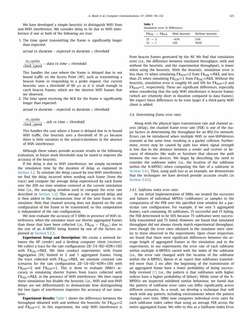
We have developed a simple heuristic to distinguish WiFi from
on-WiFi interference. We consider delay to be due to WiFi inter-
erence if one or both of the following are true:
1. The time spent transmitting the frame is significantly longer
than expected:
act ual t x durat ion − expected t x durat ion > threshold
tx _ cycles
clock _ speed − data tx time > threshold
This handles the case where the frame is delayed due to out
bound traffic on the Access Point (AP), such as transmitting a
beacon frame or responding to a probe request. Our current
heuristic uses a threshold of 60 μs as it is small enough to
catch beacon frames, which are the shortest WiFi frames that
we observed.
2. The time spent receiving the ACK for the frame is significantly
longer than expected:
act ual rx durat ion − expected rx duration > threshold
rx _ cycles
clock _ speed − ack rx time > threshold
This handles the case where a frame is delayed due to in bound
WiFi traffic. Our heuristic uses a threshold of 10 μs because
there is little variation in the actual rx durations in the absence
of WiFi interference.
Although these values provide accurate results in the following
valuation, in future work thresholds may be tuned to improve the
ccuracy of the heuristic.
If the delay is due to WiFi interference, we simply increment
he simulation time by the duration of delay as explained in
ection 3.2 . To simulate the delay caused by non-WiFi interference,
e find the delay incurred when sending each frame (from the
race) and compute the average delay experienced by each frame
ver the 200 ms time window centered at the current simulation
ime (i.e., the averaging window used to compute the error rate
escribed in Section 3.2 ). This average is the expected delay and
s then added to the transmission time of the next frame in the
imulator. Note that channel sensing does not depend on the rate
onfiguration of the frame to be transmitted, so this computation
s independent of the rate configuration.
We now evaluate the accuracy of T-SIMn in presence of WiFi in-
erference, when the simulator must use shorter aggregated frames
han those that have been collected (i.e., FA SIM < FA COL ) due to
he size of an A-MPDU being limited by one of the factors ex-
lained in Section 5.2.2 .
Experiment Setup and Description: We create a network be-
ween the AP ( sender ) and a desktop computer client ( receiver ).
e collect a trace for the rate configuration 2S-I4-SG-40M = 180ith FA COL = MAX . We then conduct experiments with Frame
ggregation (FA) limited to 2 and 1 aggregated frames. Using
he trace collected with FA COL = MAX , we simulate constant rate
cenarios for the rate configuration 2S-I4-SG-40M = 180 with
A SIM = 2 and FA SIM = 1 . This is done to evaluate SIMn’s ac-
uracy in simulating shorter frames from traces collected with
A COL = MAX , in the presence of WiFi interference. We then repeat
hese simulations but disable the heuristic (i.e., WiFi and non-WiFi
elays are not differentiated) to demonstrate how distinguishing
he two types of interference improves the accuracy of our simu-
ator.
Experiment Results: Table 1 shows the differences between the
hroughput obtained with and without the heuristic for FA SIM = 2nd FA SIM = 1 . In this experiment, the only WiFi interference is
rom beacon frames generated by the AP. We find that simulation
rror (i.e., the difference between simulated throughput, with and
ithout the heuristic, and the experimental throughput), is lower
hen using the heuristic. With the heuristic, simulation error is
ess than 1% when simulating FA SIM = 2 from FA COL = MAX , and less
han 2% when simulating FA SIM = 1 from FA COL = MAX . Without the
euristic, simulation error is roughly 6% and 10% for FA SIM = 2 and
A SIM = 1 , respectively. These are significant differences, especially
hen considering that the only WiFi interference is beacon frames
which are relatively short in duration compared to data frames).
e expect these differences to be even larger if a third-party WiFi
lient is added.
.4. Determining frame error rates
Along with the physical layer transmission rate and channel ac-
ess (delay), the channel frame error rate (FER) is one of the ma-
or factors in determining the throughput for an 802.11n network.
rrors can be introduced when multiple WiFi or non-WiFidevices
ransmit at the same time, resulting in a packet collision. Further-
ore, errors may be caused by path loss when signal strength
s low due to the distance between a sender and receiver or be-
ause of obstacles like walls or furniture that obscure the path
etween the two devices. We begin by describing the need to
onsider the subframe index (i.e., the location of the subframe
ithin the A-MPDU) when computing the fate of a subframe in
ection 5.4.1 . Then, using path loss as an example, we demonstrate
hat the techniques we have devised provide accurate results (in
ection 5.4.2 ).
.4.1. Subframe index error rates
In our initial implementation of SIMn, we treated the successes
nd failures of individual MPDUs (subframes) as samples in the
omputation of the FER over the specified time window for a par-
icular rate configuration. For example, if we sent 5 aggregated
rames, each containing 30 subframes, 15 successful and 15 failing,
he FER determined to be 50% because 75 subframes were success-
ully transmitted and 75 failed. However, we found that simulated
hroughput did not always closely match experimental throughput,
ven though the error rates obtained in the simulator were simi-
ar to those observed in the experiments. Upon closer inspection,
e found that there were significant differences between the av-
rage length of aggregated frames in the simulation and in the
xperiments. In our experiments the error rate of each subframe
ithin multiple A-MPDUs varied with the index of the subframe
i.e., the error rate changed with the location of the subframe
ithin the A-MPDU). Byeon et al. report that subframes transmit-
ed more than 2 ms after the beginning of the transmission of
n aggregated frame have a lower probability of being success-
ully received [7] (i.e., the pattern is that subframes with higher
ndices have a higher probability of failure). While some of the A-
PDUs we inspected exhibited similar behaviour, we found that
he pattern of subframe error rates can differ significantly across
ifferent scenarios. As a result, we develop a technique that will
ork with any pattern, including environments where the pattern
hanges over time. SIMn now computes individual error rates for
ach subframe index rather than using an average FER across the
ntire aggregated frame. We refer to this as a Subframe Index Error

124 A. Abedi et al. / Computer Communications 117 (2018) 116–132
Fig. 7. Impact of per-subframe error calculation.
A
Fig. 8. Mobile scenario experiencing path loss.
s
p
u
w
s
m
s
a
T
r
e
6
o
t
n
s
c
W
u
s
u
c
s
t
u
T
i
w
f
e
h
s
f
o
b
o
fi
p
i
t
n
t
I
8
3
a
c
Rate (SFIER). We now illustrate the importance of using the SFIERs
in obtaining accurate throughput in SIMn.
Experiment Setup and Description: We take advantage of an-
other feature of our trace-based simulator, namely the ability to
generate and process synthetic traces to better understand 802.11n
networks. We create two synthetic traces with equal A-MPDU frame
error rates of 41%, but using two different SFIER patterns. The equal
FERs are useful in reasoning about the expected outcome. Syn-
thetic traces are used due to the difficulty in experimentally ob-
taining traces with the same overall FER with different SFIER pat-
terns. The first trace has a linearly increasing SFIER from 0.025
at index 0 to 0.8 at index 31. The second trace uses the oppo-
site pattern, with the SFIERs decreasing linearly from 0.8 at index
0 to 0.025 at index 31. We use SIMn to simulate the transmis-
sion of frames using these two patterns and a rate configuration of
3S-I7-SG-40M = 450 . We first treat all subframe indices equally,
as in our initial implementation of SIMn. We then repeat the sim-
ulations using our current implementation of SIMn that considers
each SFIER individually and compare the throughput obtained us-
ing these two different approaches.
Experiment Results: Fig. 7 plots the throughput obtained for
the two synthetic traces. The bars on the left show the results
obtained using the current implementation with per-SFIERs and
those on the right show results obtained using the initial imple-
mentation per-SFIERs are not considered (labelled “Original”). As
expected, when using the Original implementation the throughput
of the Increasing and Decreasing patterns are equal (because they
have the same 41% FER. However, when using per-SFIERs, an in-
creasing SFIER pattern results in higher throughput than a decreas-
ing pattern, even though they have the same overall average error
rate. The decreasing SFIER pattern results in lower throughput, be-
cause failures at the start of an aggregate frame prevent the Block-
ck Window (BAW) from advancing and thus reduces the average
length of aggregated frames. These experiments illustrate the im-
pact of considering individual SFIERs and their importance in ob-
taining accurate simulation results. This is critical because our goal
is to use the simulator to evaluate link adaptation and frame ag-
gregation algorithms, which require the correct simulation of phe-
nomenon captured during trace collection.
5.4.2. Path loss
To evaluate SIMn’s ability to handle channel error rate, we use a
challenging mobile scenario where channel error rates vary widely
due to path loss.
Experiment Setup and Description: We create a network be-
tween the Access Point (AP) ( sender ) and a Mac-Book Pro (MBP).
The sender transmits for 100 seconds using constant rate config-
uration of 2S-I4-SG-40M = 180 with FA COL = MAX . We choose
this rate configuration because in this mobile scenario, its error
rates vary widely. In this experiment, the MBP is carried at walk-
ing speed in an office environment where cubicle walls obscure
line of sight. We simulate throughput for the rate configuration
2S-I4-SG-40M = 180 , using the collected trace as input to the
imulator. Note that during the simulation SFIERs must be com-
uted and frames of length shorter than the maximum will be
sed. This tests SIMn’s ability to accurately simulate throughput
ith fluctuating error rates, different error rates across different
ubframe indices, and A-MPDUs of different length.
Experiment Results: In Fig. 8 , we plot pairs of throughput
easurements, simulated and experimental, for this scenario. De-
pite the significant fluctuations during this experiment, there is
close match between simulated and experimental throughput.
his suggests that the simulator can accurately determine error
ates (including SFIERs) and simulate aggregated frames of differ-
nt lengths.
. Evaluating our framework
In the previous sections, we use constant rate traces to focus
ur tests on the T-SIMn simulator, SIMn. Although not representa-
ive of how trace collection would be done in T-SIMn, that tech-
ique is used to ensure the accuracy of SIMn on its own. In this
ection, we evaluate T-SIMn as a whole, using round-robin trace
ollection in conditions that are representative of those in which
iFi is used. For the experiments in this section, we collect traces
sing the direct measurement methodology and use an iPhone, which
upports 32 transmission rates. We show that this approach can be
sed with devices that support 32 transmission rates for easy and ac-
urate trace collection. In Section 8 , we propose and evaluate a more
ophisticated methodology that handles devices that support more
ransmission rates.
In order to evaluate the T-SIMn framework, we use an eval-
ation methodology similar to that used to evaluate T-RATE [1] .
hat is, we conduct an experiment (which produces a trace) us-
ng a round-robin ordering of rate configurations and then in SIMn
e conduct a simulation using a round-robin ordering that differs
rom the experiment. This experiment is designed as a means for
valuating the accuracy of the T-SIMn framework. The intuition be-
ind this methodology is that in both the experiments and the
imulation each rate will be used to send the same number of
rames using each rate. Therefore, the average throughput obtained
ver an interval in time from the experiment should be matched
y the average throughput obtained from the simulator. This will
nly be true if, despite not having sent a frame with rate con-
guration R at time t , the simulator can accurately determine the
robability that the frame would be successfully sent by comput-
ng the average SFIER over the channel coherence window. Addi-
ionally, different orderings means it is extremely unlikely that the
umber of frames aggregated in the simulator at time t will match
he number of aggregated frames collected in the trace at time t .
n contrast to T-RATE, we cannot cycle through all of the available
02.11n rates (96 rates for our 3 antenna devices would take about
00 ms) because the time required to perform enough rounds to
ccurately compute average error rates would exceed the channel
oherence time.

A. Abedi et al. / Computer Communications 117 (2018) 116–132 125
Fig. 9. Simulating reverse MCS ordering.
S
o
I
a
t
t
S
t
t
r
S
l
t
c
i
m
i
i
m
b
a
a
6
w
e
t
w
a
w
t
p
o
a
f
w
w
o
t
6
b
B
l
F
i
t
Fig. 10. Simulating reverse group ordering.
r
L
f
t
m
b
F
o
f
f
r
A
p
C
S
l
c
n
e
(
t
p
t
g
s
d
L
g
C
o
d
e
u
t
e
r
a
o
t
u
e
6
b
c
a
W
W
We instead limit our evaluation to one antenna (1-Spatial
tream (SS)) devices, which includes most cell phones, tablets and
ther small devices. Using Long Guard Interval (LGI), Short Guard
nterval (SGI), 20 and 40 MHz Channel Bandwidth (CB) results in
total of 32 rate configurations.
During trace collection, rates are grouped by a combination of
he Guard Interval (GI) and the CB. Therefore, rates are sampled in
he following group order LGI-20MHz , SGI-20MHz , LGI-40MHz ,GI-40MHz . Within each group, rates are sampled in order from
he lowest Modulation and Coding Scheme Index (MCS index) to
he highest (i.e., MCS index 0 , 1 , . . . , 6 , 7 ). We simulate round-
obin in the reverse group order (i.e., SGI-40MHz , LGI-40MHz ,GI-20MHz , LGI-20MHz ) and from the highest MCS index to the
owest (i.e., MCS index 7 , 6 , . . . , 1 , 0 ).
Experiment Setup and Description: We create a network be-
ween the AP ( sender ) and an iPhone 6 ( receiver ). The sender is
onfigured to sample all 32 1-SS 802.11n rate configuration, which
s the entire set of rates supported by the iPhone 6. The experi-
ent is conducted by using a mix of carrying the iPhone at walk-
ng speed and standing still in an office environment as described
n Section 4 .
Experiment Results: In Fig. 9 , we plot simulated and experi-
ental throughput. The experiment starts with the handheld mo-
ile device near the access point. The decrease in throughput from
round the 40 s econd mark to 60 s econds is due to movement
way from the access point, while the increase in throughput from
0 s econds until around 80 s econds is due to movement back to-
ard the access point. We find that simulated throughput matches
xperimental throughput except for the points at times t = 20 ,
= 60 and t = 100 . The largest difference is observed at t = 60 ,
here average simulated throughput is roughly 11% higher than
verage experimental throughput. Initially, we thought that this
as due to inaccuracy in SIMn. However, upon closer investiga-
ion, we realized that the simulator is in fact accurate and that the
roblem was with the methodology used to evaluate the accuracy
f the framework. Our assumption that simulating round-robin in
different order would result in each rate configuration being used
or the same proportion of time is not guaranteed in 802.11n net-
orks, unlike a similar evaluation we conducted for 802.11g net-
orks [1] . In the next section, we investigate and explain why the
rder in which rates are used in a round-robin fashion impacts
hroughput.
.1. Effect of rate configuration ordering
In 802.11n networks, the fate of one frame can impact the num-
er of frames that can be aggregated in the next frame due to the
lock-Ack Window (BAW). Failed aggregated frames or subframes
imit how far forward the BAW can be advanced. Recall from
ig. 1 that the number of subframes being aggregated has a signif-
cant impact on throughput, with longer aggregated frames leading
o higher potential throughput. Recall that in the previous section,
ates were sampled in the group order LGI-20MHz , SGI-20MHz ,GI-40MHz , SGI-40MHz . Additionally, rates are sampled in order
rom the lowest Modulation and Coding Scheme Index (MCS index)
o the highest (i.e., MCS index 0 , 1 , . . . , 6 , 7 ). This means that the
ost robust rates in each group are sampled first and the least ro-
ust rates are sampled last. We have examined the data shown in
ig. 9 in detail and found that at times t = 50 to 70, the reverse
rdering performed during simulation leads to longer aggregated
rames on average (a mean of 15.2 subframes in each aggregated
rame during simulation compared to 14.6 in the experiment). This
esults in slightly higher simulated throughput during this period.
lthough there is a match in simulated and experimental through-
ut during some portions of this time interval (i.e., overlapping
Is), the simulated throughputs are visibly lower for most times t .
imulating longer frames than those that were collected may also
ead to some inaccuracies because of insufficient samples in the
ollected trace for frames of the length being simulated.
As a result, we have had to revise our understanding and
ow expect different round-robin orderings to result in differ-
nt throughput, unless the behavior of the Block-Ack Window
BAW) advancement and consequently Frame Aggregation (FA) is
he same during trace collection and simulation. To test this hy-
othesis, we construct a new ordering to use in the simulation
hat preserves the property that the most robust rates in each
roup are used first and the least robust rates are used last. The
imulation still uses rate groups in the reverse order from the or-
er used when the trace is collected (i.e., simulating SGI-40MHz ,GI-40MHz , SGI-20MHz and LGI-20MHz . However, within each
roup, we now use rates in order from the lowest Modulation and
oding Scheme Index (MCS index) to the highest (i.e., the same
rder used during trace collection). We simulate a round-robin or-
ering with this new reverse group order and show simulated and
xperimental throughput in Fig. 10 . As the graph shows, the sim-
lated throughput now closely matches that obtained experimen-
ally (all pairs of confidence intervals overlap). Note that this prop-
rty does not limit SIMn to simulating only certain orderings of
ate configurations. It is only required for this evaluation of the
ccuracy of T-SIMn because we are trying to devise a methodol-
gy where the throughput of the simulator should match that of
he experiment. Now that we are aware of this property, we will
se the reverse group ordering in the following section, where we
valuate T-SIMn in an uncontrolled environment.
.2. Uncontrolled environment
Up to this point, all experiments are performed with no neigh-
oring Access Points (APs). We now move to a different 5 GHz
hannel that is in use by the university’s WiFi network to evalu-
te T-SIMn in conditions that are typical for a shared university
iFi network. This includes interference from many third-party
iFi clients and APs.

126 A. Abedi et al. / Computer Communications 117 (2018) 116–132
Fig. 11. Uncontrolled, mobile scenario.
t
b
m
h
i
m
b
q
p
d
a
t
p
c
o
7
t
d
r
r
(
e
r
s
F
k
c
s
s
p
e
c
s
d
s
d
i
t
H
n
0
i
o
p
w
c
a
t
i
a
a
r
9
w
e
t
e
fi
n
h
Experiment Setup and Description: Similarly to the previous
section, we create a network between the AP ( sender ) and an
iPhone 6 ( receiver ). However, unlike previous experiments, we now
configure the AP to use a channel occupied by one of the univer-
sity’s APs with the highest signal strength. As mentioned previ-
ously, we use a 5 GHz network because the iPhone does not sup-
port 40 MHz Channel Bandwidths (CBs) in the 2.4 GHz spectrum.
Note that if we had used the 2.4 GHz band, thus limiting trace
collection to 20 MHz rate configurations, we would have obtained
twice as many samples in each averaging window, which should
only improve accuracy. As in previous experiments, we sample all
1-Spatial Stream (SS) rate configurations. We collect a 100 s econd
trace with FA COL = MAX to test T-SIMn in an uncontrolled environ-
ment. This scenario is comprised of a mix of carrying the iPhone
at walking speed and standing still in an office and hallway envi-
ronment as explained in Section 4 .
Experiment Results: In Fig. 11 , we plot pairs of throughput
measurements, simulated and experimental, for the uncontrolled
experiment. We find that while the receiver is stationary from
= 60 to 100 there is significantly more fluctuation in throughput
when compared to Fig. 9 from t = 10 to 40 in Fig. 10 . This is due to
the third-party traffic on the shared channels. The close matches in
throughput suggest that T-SIMn is accurately capturing and simu-
lating third-party traffic and that it can handle conditions that are
representative of those in which WiFi devices are used.
7. Trace collection with many transmission rates
In Section 3.1 , we explain that the error rate of the MPDUs
within an aggregated frame are not identical. As a result, the di-
rect measurement technique measures the per MPDU error rate
by sending the longest possible A-MPDU for each transmission
rate. All transmission rates are sampled using a round-robin or-
dering. As explained in Section 3.1 , if we sample all transmission
rates within the channel coherence window, all rates experience
the same channel conditions. Since the number of transmission
rates affects the time required to complete a round of sampling
for all, this determines the number of samples that can be col-
lected within the channel coherence window. For 802.11n devices
that support many transmission rates, the number of samples col-
lected by the direct measurement technique might be too low to
accurately measure the error rate. We refer to this as the lack of
samples problem for trace collection.
In Section 6 , we show that the direct measurement technique
can be used for devices that support 32 transmission rates. How-
ever, this technique may not be accurate for devices that support
more transmission rates. For instance, for a device that supports
up to 3 spatial streams (i.e., 96 rates), our measurements have
determined that each round of sampling takes about 300 ms to
complete when using the direct measurement technique. Recall
that the channel coherence time in the 5 GHz spectrum is about
100 ms, as a result, the coherence window is 200 ms (i.e., 100 ms
efore and after a particular point in time). As a result, each trans-
ission rate only has at most one (per sub-index) sample in a co-
erence window, which may not be enough to capture fast chang-
ng channel conditions. While we have shown the direct measure-
ent methodology is accurate for 32 rates, the maximum num-
er of rates that this methodology can support depends on the re-
uired accuracy for a particular study and is a topic of future work.
However, in the rest of this section, we study the lack of sam-
les problem with the goal of alleviating the shortcomings of the
irect measurement technique. We show that a relatively intuitive
pproach that one might expect to work can not be used and argue
hat more sophisticated techniques are required. In Section 8 , we
ropose a novel methodology that can be used to obtain a suffi-
ient number of samples with devices supporting a larger number
f rates (i.e., three antennas with 96 rates).
.1. Dynamic transmission rate elimination
One approach to increasing the number of samples within
he coherence window is to dynamically eliminate “trivially pre-
ictable” transmission rates when collecting a trace using a round
obin ordering. The intuition is that if a particular transmission
ate fails to successfully transmit a frame, faster transmission rates
which use less redundancy) will not be able to transmit the frame
ither (i.e., the FER will be 1). Similarly, if a particular transmission
ate is successful, sampling slower transmission rates is not neces-
ary as they are even more robust and will be successful (i.e., the
ER will be 0). Therefore, sampling these transmission rates with
nown expected FER is wasteful and sampling all rates might be
onsidered unnecessary and “oversampling” some rates. As a re-
ult, the round robin trace collection mechanism might be able to
kip many rates and collect a larger number of more useful sam-
les by dynamically eliminating some rates.
This heuristic could solve the lack of samples problem if a large
nough portion of the rates experience an error rate sufficiently
lose to 0 or 1. These rates that are trivially predictable over some
hort periods of time (i.e., trivial rates ) can be temporarily and
ynamically excluded or included by the heuristic. Note that the
et of trivial rates might change over time as the channel con-
itions change. To evaluate the potential of such a heuristic, we
nitially designed an experiment to examine the number of non-
rivial rates , with FER � = 0 or FER � = 1, over a one second window.
owever, we soften those requirements to reduce the number of
on-trivial rates by considering only rates with an FER between
.05 and 0.95 as non-trivial. If the intuition behind the heuristic
s correct, a small portion of rates will be non-trivial and the rest
f them will be trivial and can therefore be eliminated from sam-
ling.
In this experiment, a laptop (i.e., receiver) equipped with the
ireless N USB adapter, which supports 96 transmission rates, is
arried at walking speeds for 15 minutes in the office environment
s described in Section 4 . There exists no line-of-sight between
he AP and client for most of the experiment, because the signal
s blocked by obstacles such as metal cabinets, cubicle partitions
nd walls. We use a 2.4 GHz channel, which is exposed to WiFi
nd non-WiFi interference. The distance between the AP and client
anges from 1 meter to about 20 meters. In this experiment, all
6 transmission rates are sampled using a round robin ordering
ithout frame aggregation. Frame aggregation is not used in this
xperiment to increase the number of samples collected for each
ransmission rate.
Fig. 12 shows the number of non-trivial rates that cannot be
liminated by the heuristic over the 15 minute experiment. The
gure indicates that there are several times when the number of
on-trivial rates is more than 70. Therefore, at those times the
euristic can eliminate less than 26 of the 96 transmission rates.

A. Abedi et al. / Computer Communications 117 (2018) 116–132 127
Fig. 12. Mobile 2.4 GHz.
Fig. 13. Mobile 5 GHz.
S
2
p
b
s
m
r
e
s
f
s
p
e
t
n
m
o
i
A
n
a
o
8
i
m
c
i
o
r
f
f
o
g
m
l
o
Fig. 14. Impact of speed on MPDU delivery ratio.
M
d
a
f
i
s
8
(
t
c
h
t
n
s
s
l
t
S
n
f
p
5
M
t
t
d
d
b
t
n
i
i
2
a
ampling 70 transmission rates using frame aggregation takes over
00 ms to complete. As a result, each rate has at most one sam-
le over the coherence windows (i.e., 200 ms) and this heuristic,
ased on dynamic rate elimination, will also suffer from a lack of
amples. Therefore, we dismiss this as a potential trace collection
ethodology. We believe that the reason for these counterintuitive
esults is WiFi and non-WiFi interference. We believe that interfer-
nce might be strong enough to change the FER of most transmis-
ion rates regardless of the amount of redundancy encoded in the
rames.
To support this claim, we repeat the experiment in the 5 GHz
pectrum on a channel with no WiFi or non-WiFi interference and
resent the results in Fig. 13 . Note that except the spectrum band,
verything else in this experiment is unchanged. Fig. 13 indicates
hat when the interference is eliminated from the experiment, the
umber of non-trivial rates decreases significantly.
In summary, the rate elimination heuristic might be able to skip
any transmission rates when there is no interference. However,
ur goal is to collect traces under a variety of channel conditions
ncluding those that are affect by different sources of interference.
s a result, this heuristic cannot be used for our purpose. In the
ext section, we characterize the MPDU delivery ratio patterns in
n A-MPDU and then use the characterization to design a method-
logy for collecting traces with many transmission rates.
. Inferred measurement technique
The Frame Error Rate (FER) is not identical for the MPDUs
n an aggregated frame. For this reason, the direct measurement
ethodology, transmits the largest possible A-MPDU, during trace
ollection, to measure the FER of all MPDU indexes. However, us-
ng frame aggregation during trace collection leads to the lack
f samples problem in 802.11n networks with many transmission
ates as explained in Section 7 . We now describe our new in-
erred measurement methodology, which avoids frame aggregation
or trace collection to increase the number of samples collected
ver the channel coherence window. Note that when frame aggre-
ation is disabled, only the error rate of the first MPDU can be
easured. Since during simulation an A-MPDU with any arbitrary
ength might be transmitted, the inferred measurement method-
logy needs to accurately estimate the error rate of the missing
PDUs. To explain the design of this methodology, we need to un-
erstand the characteristics of the MPDU delivery ratio (MDR) in
n aggregated frame. Therefore, we first study the effect of carrier
requency and the speed of movement on the changes to the MDR
n an A-MPDU, then, we describe the design of the inferred mea-
urement technique.
.1. Changes of MDR in an A-MPDU
Byeon et al. [7] report that if channel conditions change rapidly
for instance when the sender or receiver is moving), subframes at
he end of an A-MPDU experience higher error rates than those
loser to the header of the frame. In addition, they show that
igher speeds of movement intensify this phenomenon. In order
o accurately estimate the MDR of subframes in an A-MPDU, we
eed to characterize and understand how the MDR of different
ubframes change within an A-MPDU. In this section, the MDR of
ubframe i is denoted by MDR i .
We design a mobile experiment where a laptop with the wire-
ess N USB adapter is carried at different speeds from a very slow
o a fast walking speed in the office environment described in
ection 4 . We divide the experiment into three parts, namely, slow,
ormal, and fast walking speeds.
Fig. 14 shows the relative MPDU delivery ratio (relative MDR)
or the physical rate of 117 Mbps for the three walking speeds. We
resent the relative MDR for an easier comparison of the 2.4 and
GHz experiments. The relative MDR is computed by dividing the
DR of each index by the MDR of the first MPDU. For instance,
he relative MDR of subframe i is MDRi / MDR 1 . We can observe
hat in both spectrums as the speed increases the delivery ratio
rops more sharply due to more rapid changes in the channel con-
itions, this is because the initial calibrations done on the pream-
le are less representative of the channel state as the time since
he preamble increases. The results show that the speed has a sig-
ificant role in the decrease of the MDR and it is more prominent
n the 5 GHz spectrum. For instance, let’s consider MPDUs with
ndex 16, which are in the middle of the aggregated frames. In the
.4 GHz spectrum, the relative MDR at the slow and fast speeds
re 0.84 and 0.48, respectively. The relative MDR had dropped by

128 A. Abedi et al. / Computer Communications 117 (2018) 116–132
Fig. 15. Channel dynamics indicator.
C
c
s
t
8
p
n
M
o
o
m
b
c
t
s
w
g
t
i
c
i
s
M
∀
w
m
n
t
a
t
u
i
t
n
t
g
w
c
m
t
s
M
2 The ath9k driver limits the transmission time to 4 ms to comply with the chan-
nel occupancy restriction at the 5 GHz ISM spectrum.
43%, while in the 5 GHz band, the relative MDR is 0.64 and 0.02,
which is a 97% drop. Byeon et al. [7] also observed that the speed
of movement intensifies the MDR decline phenomenon. However,
their measurements are conducted in the 5 GHz spectrum only.
Our results show that the 2.4 and 5 GHz frequency bands impact
this phenomenon differently.
One reason for the faster decrease of the MPDU delivery ratio
in the 5 GHz spectrum is explained by the Doppler shift. The fol-
lowing formula shows how the Doppler shift is directly related to
the transmission frequency ( f 0 ):
� f =
(�v c
)f 0 (2)
where �f is the frequency shift, �v is the relative speed of the
sender and receiver, and c is the speed of light. As Eq. (2) indi-
cates, for a given relative speed �v , the frequency shift in the 5
GHz spectrum is almost twice that of the 2.4 GHz spectrum. The
frequency shift due to the Doppler effect causes inter-subcarrier
interference in OFDM communication systems, which consequently
increases the bit error rate leading to a higher FER. As a result, in
the 5 GHz spectrum, the later MPDUs in an aggregated frame are
more likely to observe a change in the channel conditions (i.e., fre-
quency shift) due to a stronger Doppler effect.
We observe that the MDR decline patterns are related to the speed
of movement. If we can quantify the channel dynamics caused by the
movement of the sender, receiver, or nearby objects, we might be able
to estimate the MDR of all other MPDUs from the MDR of the first
MPDU and the channel dynamics metric.
The inferred measurement methodology (explained later in this
section) utilizes this idea by turning off frame aggregation dur-
ing trace collection (i.e., measuring the MDR of the first MPDU
only) and estimating the MDR of missing MPDUs. By not using
frame aggregation, the inferred measurement methodology can
collect more samples during the same time interval than the di-
rect measurement technique. We show that the inferred measure-
ment methodology is able to support 802.11n networks with many
transmission rates (in this case up to 96). We next describe a novel
technique for quantifying the channel dynamics, then we present
the design of the inferred measurement methodology.
8.2. Channel dynamics indicator (CDI)
We have shown that the decline of the MPDU delivery ratio in
an aggregated frame depends on the speed of movement. We now
propose measuring the channel dynamics (which changes with the
speed of movement) by using changes in the RSSI of ACKs. Note
that we do not use RSSI to estimate the frame error rate, instead,
we infer the channel dynamics from the changes in the measured
RSSI.
We require a statistical measure that reflects the channel dy-
namics. In other words, this metric should change with the speed
or amount of movement of the sender, receiver, and the sur-
rounding objects. We will use this measure to estimate how the
MDR declines as the subframe index increases (i.e., how later
frames within the A-MPDU have higher error rates). We found that
the variance of the difference between consecutive RSSI measure-
ments, which we call Channel Dynamics Indicator (CDI) , is a suitable
measure. Studying other statistical measures will be the subject of
future work.
Fig. 15 shows the channel dynamics indicator for the experi-
ment we described in Section 8.1 . In this experiment, the speed
of movement increases gradually during the experiment, therefore,
we expect that the channel dynamics indicator to change in con-
junction with the speed of movement. The graph shows that our
metric correctly increases with the movement speed. At the begin-
ning of the experiment, when the movement speed is very low, the
DI is fairly close to zero. As the speed increases, the CDI also in-
reases to reflect the more variable channel conditions. In the next
ection, we show how this metric can be utilized to accurately es-
imate the MPDU delivery ratios.
.3. Inferred measurement methodology
We observed that the channel dynamics indicator (CDI) can
otentially be a good estimator for the fluctuations in the chan-
el conditions caused by mobility. We have also shown that the
PDU delivery ratio decline in an A-MPDU depends on the speed
f movement. As a result, we hypothesize that if the delivery ratio
f the first MPDU of a given A-MPDU and the CDI can be deter-
ined, the delivery ratio of other MPDUs in that A-MPDU could
e estimated. If this hypothesis turns out to be true, then we can
ollect traces without frame aggregation and infer the delivery ra-
io of missing MPDUs from non-aggregated frames (which corre-
pond to the first MPDU in an A-MPDU) and CDI. In other words,
e can increase the number of samples by not using frame aggre-
ation, but still estimate the delivery ratio of all MPDUs, emulating
he case where traces are collected using frame aggregation.
We now show that for the traces studied, the channel dynamics
ndicator and the delivery ratio of the first MPDU (MDR 1 ) can ac-
urately estimate the delivery ratio of other MPDUs (MDR i ), where
is the MPDU index. In general, we observe that for each transmis-
ion rate, there exists a function f i that maps the CDI and MDR 1 to
DR i :
i ∈ { 1 , 2 , . . . , M AX } ∃ f i : (M DR 1 , CDI) → M DR i (3)
here MAX is the maximum number of MPDUs that can be trans-
itted in 4 ms 2 . Note that the ath9k driver further limits the
umber of MPDUs to 32.
Fig. 16 illustrates how the channel dynamics indicator (CDI) and
he MDR of the first MPDU (MDR 1 ) is related to MDR 16 (bottom)
nd MDR 32 (top), for the experiment described in Section 8.1 . In
his experiment, a laptop is carried at various speeds for 15 min-
tes in the office environment.
The results for the physical layer transmission rate of 117 Mbps
s presented in the graph. Similar results were observed for other
ransmission rates. As depicted in the figure, when the channel dy-
amics indicator increases (i.e., corresponding to faster movement)
he MPDU delivery ratios of MPDUs 16 and 32 decrease for any
iven MDR 1 . This is in line with our findings in Section 8.1 where
e observed that the MDR drops more rapidly as the speed in-
reases. MDR 16 and MDR 32 are relatively high when the receiver
oves very slowly (i.e., CDI < 1) and MDR 1 is high (e.g., due
o good channel conditions for the given modulation and coding
cheme). As expected, MDR 16 is generally higher than MDR 32 as
PDUs closer to the frame header have a higher delivery ratio.

A. Abedi et al. / Computer Communications 117 (2018) 116–132 129
Fig. 16. Channel dynamics indicator.
Fig. 17. Inferred measurement methodology.
8
m
i
o
A
t
f
o
f
n
t
o
f
s
m
a
o
s
i
t
w
p
s
m
p
w
t
l
c
.3.1. Methodology overview
In order to enable trace collection using devices that support
any transmission rates we have designed and implemented the
nferred measurement methodology. The overview of our method-
logy (illustrated in Fig. 17 ) is as follows:
1. A calibration trace is collected using frame aggregation, using
the direct measurement technique explained in Section 3.1 .
This trace is used to find the relationships between the CDI and
MDRs. To compute the MDRs, we use 10-second windows to
obtain enough samples to accurately measure the MDRs (i.e., up
to 30 samples inside the averaging window). Note that the goal
is not to measure the MDRs at a particular time but rather to
compute the relationships between the CDI and MDRs. There-
fore, in this case, the averaging window does not need to be
smaller than or equal to the channel coherence time.
2. A main trace is collected without using frame aggregation (i.e.,
FA COL = 1 ). This trace is called the main trace because it is a trace of the
experiment and environment that will be later used in the sim-
ulation (i.e., it is the experiment that will be simulated). The
MDR 1 and CDI information from this trace along with the map-
ping functions (obtained from the calibration trace) are used in
the next step to find the fate of missing MPDUs.
3. For each transmission rate and subframe index i , the calibration
trace gives us a set of 3-tuples, MDR 1 , MDR i , and CDI, which
creates a 3D surface (i.e., mapping function ) as previously shown
in Fig. 16 . We use multi-variable regression, where MDR 1 and
CDI are the estimator variables and MDR i is the estimated vari-
able, to determine this mapping function (details are presented
later in this section). This procedure is repeated for all trans-
mission rates and subframe indexes.
4. In order to estimate the fate of missing MPDUs in the main
trace, we use the following procedure: for a given frame in
the main trace at time t and transmission rate R , we consider
a time window centered at time t and compute the average
MDR of MPDU 1 (i.e., MDR 1 ) from the frames with rate R in
this window. The time window we use in this study is 200 ms
to roughly approximate the channel coherence time. Similarly,
we compute the CDI from the RSSI of all ACKs, regardless of
the transmission rate, in this window. Note that the RSSI is a
property of an electromagnetic signal not the transmission rate.
Then, we use the computed MDR 1 and CDI as input into the
mapping functions to estimate the expected fate of the MPDUs
missing from the main trace. This procedure is repeated for all
frames in the main trace and the results are stored in the gen-
erated trace . The generated trace is similar to the output of the
direct measurement methodology, except that in this case the
MPDU fates are estimated (or inferred by applying the models
obtained from the calibration trace to the frames obtained in
the main trace). This generated trace is used by T-SIMn to con-
duct performance evaluations.
Note that both calibration and main traces include the RSSI of
CKs needed to compute the CDI. In the inferred measurement
echnique, the calibration trace is only used to find the mapping
unctions. These mapping functions are used to estimate the fate
f missing MPDUs in the main trace and can be used with dif-
erent main traces in that environment, therefore, they do not
eed to be recalculated for each new main trace. Then, the main
race is actually used for performance evaluation. The advantage
f this methodology is that the main trace contains many more
rames per unit of time than can be collected using the direct mea-
urement methodology. For example, in the inferred measurement
ethodology, if all 96 transmission rates (in a 3x3 MIMO system)
re sampled using a round robin sampling technique, we obtain
ne sample every 43 ms for each transmission rate (i.e., about 5
amples over a 200 ms coherence window). This is a large gain
n terms of the number of samples collected when compared with
race collection using frame aggregation (i.e., direct measurement)
here we sample each rate every 300 ms (i.e., less than one sam-
le over a 200 ms coherence window). As a result, for devices that
upport 3 spatial streams (i.e., 96 transmission rates),the inferred
easurement methodology increases the number of collected sam-
les to 5 samples over the 200 ms coherence window, compared
ith only 0.7 samples that would be obtained if we were to use
he direct measurement methodology. While 5 samples may seem
ow, we show that the inferred measurement methodology can ac-
urately estimate the fate of missing MPDUs.

130 A. Abedi et al. / Computer Communications 117 (2018) 116–132
Fig. 18. Inferred measurement methodology evaluation procedure.
n
s
b
p
i
T
t
e
m
d
t
u
a
W
s
t
s
Eq. (4) shows the regression model used in this study to ob-
tain the mapping functions from the calibration trace. The model
that we use contains two predictor terms MDR 1 and CDI . In addi-
tion, it has quadratic and interaction terms. We now explain why
we include these terms in the model. Fig. 16 shows that the re-
lation between the predictor terms (i.e., MDR 1 and CDI ) is curvi-
linear with MDR i . As a result, we add the quadratic terms to the
regression model. For the traces used in this study, we did not
find higher order terms necessary in the regression model. In ad-
dition, as can be seen in Fig. 16 , there are interactions between
the predictor terms. For example, when CDI = 4 , the relation be-
tween MDR 1 and MDR 32 is almost constant (i.e., MDR 32 ≈ 0). On
the other hand, when CDI = 0 , MDR 32 is a curvilinear function of
MDR 1 . This observation confirms the existence of interactions be-
tween the predictors. As a result, we add the MDR 1 ∗CDI term to
Eq. (4) to model the interactions between MDR 1 and CDI . We will
show that the regression model in Eq. (4) works well for the pur-
pose of this study, however, we plan to examine other possible
models in future work.
MDR i = β0 + β1 MDR 1 + β2 CDI
+ β3 MDR 1 2 + β4 CDI 2
+ β5 (MDR 1 ∗ CDI)
(4)
8.4. Methodology evaluation
To evaluate the efficacy of the inferred measurement method-
ology one can compare the outcome of this technique with that
of an actual experiment (i.e., the ground truth). However, it re-
quires repeatability between the trace collection and the ground
truth experiment and achieving repeatability is very difficult, es-
pecially in environments that involve mobility and interference. As
noted previously, our goal is to be able to simulate environments
with mobility and interference. Therefore, we design a novel tech-
nique, illustrated in Fig. 18 , to study the accuracy of the inferred
measurement methodology. Instead of using the main trace, which
contains samples for all rates, we collect a trace (called a test trace)
for a given transmission rate by alternatively sending frames with
and without frame aggregation. The frames without frame aggre-
gation serve as the input to inferred measurement methodology,
while the aggregated frames are used to determine ground truth.
The frames without frame aggregation are down-sampled before
being fed to the inferred measurement methodology to match the
umber of samples obtained normally when sampling all transmis-
ion rates (i.e., matching the number of usable frames that would
e available in the main trace). With this approach, we run an ex-
eriment in a way that it gives us the ground truth data and the
nput to the inferred measurement methodology simultaneously.
he inferred measurement methodology should be able to use only
hose non-aggregated frames to accurately estimate the fate of
ach MPDU in aggregated frames. Remember that with the inferred
easurement methodology, in order to collect the main trace, we
isable frame aggregation to increase the number of samples ob-
ained per unit time. Then, we infer the fate of aggregated frames
sing the mapping functions (obtained from the calibration trace)
nd the main trace (which contains non-aggregated frames only).
e now explain the procedure for evaluating the inferred mea-
urement methodology step by step as illustrated in Fig. 18 . Note
hat some steps are identical to what is done in the inferred mea-
urement methodology (marked as [IDENTICAL]).
1. Collect a calibration trace as explained before (i.e., round robin
all transmission rates with FA COL = MAX ). [IDENTICAL]
2. Collect a test trace for a given transmission rate R. Frame aggre-
gation is turned on and off alternatively (i.e., FA COL = MAX and
FA COL = 1 ) for each physical frame. Aggregated frames are ex-
tracted from the test trace and are stored in the ground truth
trace , while non-aggregated frames are stored in the single-rate
main trace . As opposed to the main trace, which is normally
collected when using the inferred measurement methodology
(containing the fate of all rates), this single-rate main trace con-
tains the fate of rate R only. Note that for the purpose of eval-
uating the inferred measurement methodology, instead of sam-
pling all rates, we sample only one rate so that we can also
collect the ground truth data (i.e., aggregated frames) simulta-
neously.
3. For each transmission rate, mapping functions f i are computed
using the regression model in Eq. (4) based on the calibration
trace MDRs and CDI data [IDENTICAL].
4. To estimate the MDR of missing MPDUs, the MDR 1 and CDI
from the single-rate main trace are used as input into the map-
ping functions, which are used to produce the single-rate gener-
ated trace .
5. The single-rate generated trace and ground truth traces are fed
separately to T-SIMn. T-SIMn is configured to saturate the link
with a UDP stream using the constant physical layer rate R.
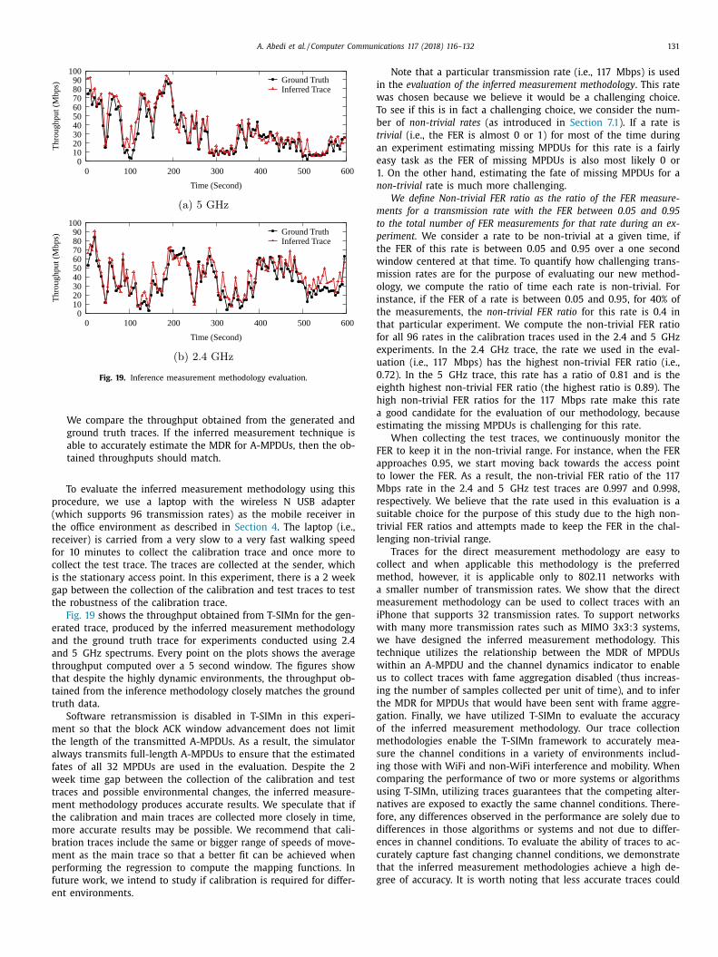
A. Abedi et al. / Computer Communications 117 (2018) 116–132 131
Fig. 19. Inference measurement methodology evaluation.
p
(
t
r
f
c
i
g
t
e
a
a
t
t
t
t
m
t
a
f
w
t
m
t
m
b
m
p
f
e
i
w
T
b
t
a
e
1
n
m
t
p
t
w
m
o
i
t
t
f
e
u
0
e
h
a
e
F
a
t
M
r
s
t
l
c
m
a
m
i
w
w
t
w
u
i
t
g
o
m
s
i
c
u
n
f
d
e
c
t
g
We compare the throughput obtained from the generated and
ground truth traces. If the inferred measurement technique is
able to accurately estimate the MDR for A-MPDUs, then the ob-
tained throughputs should match.
To evaluate the inferred measurement methodology using this
rocedure, we use a laptop with the wireless N USB adapter
which supports 96 transmission rates) as the mobile receiver in
he office environment as described in Section 4 . The laptop (i.e.,
eceiver) is carried from a very slow to a very fast walking speed
or 10 minutes to collect the calibration trace and once more to
ollect the test trace. The traces are collected at the sender, which
s the stationary access point. In this experiment, there is a 2 week
ap between the collection of the calibration and test traces to test
he robustness of the calibration trace.
Fig. 19 shows the throughput obtained from T-SIMn for the gen-
rated trace, produced by the inferred measurement methodology
nd the ground truth trace for experiments conducted using 2.4
nd 5 GHz spectrums. Every point on the plots shows the average
hroughput computed over a 5 second window. The figures show
hat despite the highly dynamic environments, the throughput ob-
ained from the inference methodology closely matches the ground
ruth data.
Software retransmission is disabled in T-SIMn in this experi-
ent so that the block ACK window advancement does not limit
he length of the transmitted A-MPDUs. As a result, the simulator
lways transmits full-length A-MPDUs to ensure that the estimated
ates of all 32 MPDUs are used in the evaluation. Despite the 2
eek time gap between the collection of the calibration and test
races and possible environmental changes, the inferred measure-
ent methodology produces accurate results. We speculate that if
he calibration and main traces are collected more closely in time,
ore accurate results may be possible. We recommend that cali-
ration traces include the same or bigger range of speeds of move-
ent as the main trace so that a better fit can be achieved when
erforming the regression to compute the mapping functions. In
uture work, we intend to study if calibration is required for differ-
nt environments.
Note that a particular transmission rate (i.e., 117 Mbps) is used
n the evaluation of the inferred measurement methodology . This rate
as chosen because we believe it would be a challenging choice.
o see if this is in fact a challenging choice, we consider the num-
er of non-trivial rates (as introduced in Section 7.1 ). If a rate is
rivial (i.e., the FER is almost 0 or 1) for most of the time during
n experiment estimating missing MPDUs for this rate is a fairly
asy task as the FER of missing MPDUs is also most likely 0 or
. On the other hand, estimating the fate of missing MPDUs for a
on-trivial rate is much more challenging.
We define Non-trivial FER ratio as the ratio of the FER measure-
ents for a transmission rate with the FER between 0.05 and 0.95
o the total number of FER measurements for that rate during an ex-
eriment. We consider a rate to be non-trivial at a given time, if
he FER of this rate is between 0.05 and 0.95 over a one second
indow centered at that time. To quantify how challenging trans-
ission rates are for the purpose of evaluating our new method-
logy, we compute the ratio of time each rate is non-trivial. For
nstance, if the FER of a rate is between 0.05 and 0.95, for 40% of
he measurements, the non-trivial FER ratio for this rate is 0.4 in
hat particular experiment. We compute the non-trivial FER ratio
or all 96 rates in the calibration traces used in the 2.4 and 5 GHz
xperiments. In the 2.4 GHz trace, the rate we used in the eval-
ation (i.e., 117 Mbps) has the highest non-trivial FER ratio (i.e.,
.72). In the 5 GHz trace, this rate has a ratio of 0.81 and is the
ighth highest non-trivial FER ratio (the highest ratio is 0.89). The
igh non-trivial FER ratios for the 117 Mbps rate make this rate
good candidate for the evaluation of our methodology, because
stimating the missing MPDUs is challenging for this rate.
When collecting the test traces, we continuously monitor the
ER to keep it in the non-trivial range. For instance, when the FER
pproaches 0.95, we start moving back towards the access point
o lower the FER. As a result, the non-trivial FER ratio of the 117
bps rate in the 2.4 and 5 GHz test traces are 0.997 and 0.998,
espectively. We believe that the rate used in this evaluation is a
uitable choice for the purpose of this study due to the high non-
rivial FER ratios and attempts made to keep the FER in the chal-
enging non-trivial range.
Traces for the direct measurement methodology are easy to
ollect and when applicable this methodology is the preferred
ethod, however, it is applicable only to 802.11 networks with
smaller number of transmission rates. We show that the direct
easurement methodology can be used to collect traces with an
Phone that supports 32 transmission rates. To support networks
ith many more transmission rates such as MIMO 3x3:3 systems,
e have designed the inferred measurement methodology. This
echnique utilizes the relationship between the MDR of MPDUs
ithin an A-MPDU and the channel dynamics indicator to enable
s to collect traces with fame aggregation disabled (thus increas-
ng the number of samples collected per unit of time), and to infer
he MDR for MPDUs that would have been sent with frame aggre-
ation. Finally, we have utilized T-SIMn to evaluate the accuracy
f the inferred measurement methodology. Our trace collection
ethodologies enable the T-SIMn framework to accurately mea-
ure the channel conditions in a variety of environments includ-
ng those with WiFi and non-WiFi interference and mobility. When
omparing the performance of two or more systems or algorithms
sing T-SIMn, utilizing traces guarantees that the competing alter-
atives are exposed to exactly the same channel conditions. There-
ore, any differences observed in the performance are solely due to
ifferences in those algorithms or systems and not due to differ-
nces in channel conditions. To evaluate the ability of traces to ac-
urately capture fast changing channel conditions, we demonstrate
hat the inferred measurement methodologies achieve a high de-
ree of accuracy. It is worth noting that less accurate traces could
132 A. Abedi et al. / Computer Communications 117 (2018) 116–132
[
[
[
still be used to evaluate competing alternatives as they would be
compared using the same trace.
9. Conclusions
In this paper, we design a trace-based simulation framework for
802.11n networks, called T-SIMn. We find that carefully consider-
ing all factors that affect throughput such as 802.11n transmission
features, channel access, and channel error rate are necessary to
accurately simulate this standard. More specifically, we show that
accurate handling of 802.11n frame aggregation is a key in obtain-
ing realistic and high fidelity results. We demonstrate that SIMn
accurately simulates these factors by comparing the simulator re-
sults with empirical measurements.
We design and evaluate two trace collection methodologies,
namely, direct measurement and inferred measurement tech-
niques. Using the direct measurement methodology, we demon-
strate that the T-SIMn framework can be used with 1 antenna de-
vices (which includes most smart phones and tablets). Finally, we
show that the inferred measurement technique enables the frame-
work to work with devices that support many transmission rates
such as MIMO 3x3:3 systems.
We have implemented the frame aggregation and Minstrel HT
rate adaptation algorithms from the ath9k driver in our simulator.
In addition, we have implemented the MoFA frame aggregation al-
gorithm [7] , are currently working on the STRALE rate adaptation
and frame aggregation algorithms [26] and plan to add more algo-
rithms. We plan to use T-SIMn to conduct a comprehensive evalu-
ation of existing link adaptation and frame aggregation algorithms
using a wide variety of environments. Additionally, as part of our
future work, we plan to compare the accuracy of T-SIMn with that
of simulators like ns-3and OMNeT ++ . We believe that T-SIMn is a
valuable tool for the realistic and repeatable performance evalua-
tion of 802.11n networks. To that end, we have made some traces
available [27] and intend to add more traces and T-SIMn to this
repository.
Acknowledgments
Funding for this project was provided in part by a Natural Sci-
ences and Engineering Research Council (NSERC) of Canada Discov-
ery Grant and a Discovery Accelerator Supplement in addition to
an NSERC Graduate Scholarship. The authors thank Martin Karsten,
Srinivasan Keshav and the anonymous reviewers for their helpful
feedback on previous revisions of this work.
References
[1] A. Abedi , T. Brecht , T-RATE: A framework for the trace-driven evaluation of802.11 rate adaptation algorithms, MASCOTS, 2014 .
[2] L. Kriara , M.K. Marina , SampleLite: a hybrid approach to 802.11n link adapta-tion, ACM SIGCOMM Comput. Commun. Rev. 45 (2) (2015) 4–13 .
[3] L. Deek , E. Garcia-Villegas , E. Belding , S.-J. Lee , K. Almeroth , A practical frame-work for 802.11 MIMO rate adaptation, Comput. Netw. 83 (2015) 332–348 .
[4] Z. Zhao , F. Zhang , S. Guo , X.-Y. Li , J. Han , RainbowRate: MIMO rate adaptationin 802.11n WiLD links, in: Proceedings of the IPCCC, 2014 .
[5] L. Deek , E. Garcia-Villegas , E. Belding , S.-J. Lee , K. Almeroth , Intelligent chan-nel bonding in 802.11n WLANs, IEEE Trans. Mob. Comput. 13 (6) (2014)
1242–1255 .
[6] P. Huang , X. Yang , L. Xiao , Adaptive channel bonding in multicarrier wirelessnetworks, in: Proceedings of the MobiHoc, 2013 .
[7] S. Byeon , K. Yoon , O. Lee , S. Choi , W. Cho , S. Oh , MoFA: mobility-aware frameaggregation in Wi-Fi, in: Proceedings of the CoNEXT, 2014 .
[8] P. Teymoori , A. Dadlani , K. Sohraby , K. Kim , An optimal packet aggregationscheme in delay-constrained IEEE 802.11n WLANs, in: Proceedings of the
WiCOM, 2012 .
[9] A. Abedi , A. Heard , T. Brecht , Conducting repeatable experiments and fair com-parisons using 802.11n MIMO networks, ACM SIGOPS 49 (1) (2015) 41–50 .
[10] R. Burchfield , E. Nourbakhsh , J. Dix , K. Sahu , S. Venkatesan , R. Prakash , RFin the jungle: effect of environment assumptions on wireless experiment re-
peatability, in: Proceedings of the ICC, 2009 . [11] M. Lacage , T.R. Henderson , Yet another network simulator, Proceeding from the
2006 Workshop on ns-2: The IP Network Simulator, ACM, 2006 .
[12] A. Varga , R. Hornig , An overview of the OMNeT ++ simulation environment, in:Proceedings of the 1st International Conference on Simulation Tools and Tech-
niques for Communications, Networks and Systems & Workshops, in: Simu-tools ’08, 2008, pp. 60:1–60:10 .
[13] R. Technology, SteelCentral Riverbed Modeler, 2016, http://www.riverbed.com/products/steelcentral/steelcentral-riverbed-modeler.html .
[14] Scalable Network Technologies, Inc., QualNet, 2014, http://web.
scalable-networks.com/qualnet . [15] M. Stoffers , G. Riley , Comparing the ns-3 propagation models, in: Proceedings
of the MASCOTS, IEEE, 2012, pp. 61–67 . [16] INET Framework for OMNeT ++ , January 22, 2016, 2016 https://omnetpp.org/
doc/inet/api-current/inet-manual-draft.pdf . [17] G. Judd , P. Steenkiste , Repeatable and realistic wireless experimentation
through physical emulation, SIGCOMM Comput. Commun. Rev. 34 (1) (2004)
63–68 . [18] G. Judd , P. Steenkiste , Using emulation to understand and improve wireless
networks and applications, in: Proceedings of the NSDI, 2005 . [19] J. Zhou , Z. Ji , R. Bagrodia , TWINE: A hybrid emulation testbed for wireless net-
works and applications., in: Proceedings of the INFOCOM, 2006 . [20] D. Halperin , W. Hu , A. Sheth , D. Wetherall , Predictable 802.11 packet delivery
from wireless channel measurements, ACM SIGCOMM Comput. Commun. Rev.
41 (4) (2011) 159–170 . [21] D. Kotz , C. Newport , R.S. Gray , J. Liu , Y. Yuan , C. Elliott , Experimental evaluation
of wireless simulation assumptions, in: Proceedings of the MSWiM, 2004 . 22] V. Lenders , M. Martonosi , Repeatable and realistic experimentation in mobile
wireless networks, IEEE Trans. Mob. Comput. 8 (12) (2009) 1718–1728 . 23] W.-L. Shen , Y.-C. Tung , K.-C. Lee , K.C.-J. Lin , S. Gollakota , D. Katabi , M.-S. Chen ,
Rate adaptation for 802.11 multiuser MIMO networks, in: Proceedings of theMobicom, 2012 .
[24] J.G. Andrews , A. Ghosh , R. Muhamed , Fundamentals of WiMAX-Understanding
Broadband Wireless Networking, Prentice Hall, Upper Saddle River, NJ, 2007 . 25] A. Heard , T-SIMn: Towards a Framework for the Trace-Based Simulation of
802.11n Networks, University of Waterloo, 2016 Master’s thesis . [26] S. Byeon , K. Yoon , C. Yang , S. Choi , STRALE: mobility-aware PHY rate and frame
aggregation length adaptation in WLANs, in: Proceedings of the Infocomm,2017 .
[27] Sample traces, https://cs.uwaterloo.ca/ ∼brecht/t-simn .