NUMERICAL MODELING OF UNSTEADY AND NON-EQUILIBRIUM SEDIMENT TRANSPORT IN

RIVERS

A Thesis Submitted to The Graduate School of Engineering and Sciences of

İzmir Institute of Technology In Partial Fulfillment of the Requirements for the Degree of

MASTER OF SCIENCE

in Civil Engineering

by Aslı BOR

December 2008

İZMİR

We approve the thesis of Aslı BOR Prof. Dr. Gökmen TAYFUR Supervisor Department of Civil Engineering İzmir Institute of Technology Asist. Prof. Dr. Şebnem ELÇİ Department of Civil Engineering İzmir Institute of Technology Prof. Dr. M. Şükrü GÜNEY Department of Civil Engineering Dokuz Eylül University ….. …. …… ….. 04.12.2008 Date

Prof. Dr. Hasan BÖKE

Dean of the Graduate School of Engineering and Science

Prof. Dr. Gökmen TAYFUR Head of the Department of Civil Engineering

ACKNOWLEDGEMENTS

I would like to thank my advisor Prof. Dr. Gökmen TAYFUR for making this

work possible. I am very grateful for his constant guidance, support and encouragement

throughout my masters program. I would like to extend a note of thanks to Asst. Prof.

Dr. Şebnem ELÇİ for taking her valuable time out and agreeing to be on my thesis

committee and also helping me out in times of need.

This study would not be possible without the support of The Scientific and

Technical Research Council of Turkey (TUBİTAK Project number 106M274). I also

would like to special thanks to Prof. Dr. M. Şükrü GÜNEY, who is the principle

investigator of the project and he is the member of thesis committee for his valuable

assistance throughout this project. I would also like to thank Prof. Dr. Turhan ACATAY

and Gökçen BOMBAR for all the assistance they have provided.

Thanks to research assistants at IYTE Department of Civil Engineering who

helped me in anyway along this study. Thanks to my colleagues Anıl ÇALIŞKAN,

Ramazan AYDIN and Sinem ŞİMŞEK for their help. Also special thanks to Nisa

KARTALTEPE for her encouragement and good friendship.

I would like to extend a note of thanks to my sister Gizem BOR, my cousins

Alptuğ TATLI, Altuğ TATLI and İsmail KESKİN for all their continuous support and

endless love. A special thank to Fatih YAVUZ for his assistance and encouragement.

Finally, I would like to give a special thanks to my parents and all other extend family

members for their love and support, which always inspired me through my research

period.

iv

ABSTRACT

NUMERICAL MODELING OF UNSTEADY AND NON-EQUILIBRIUM SEDIMENT TRANSPORT IN RIVERS

Management of soil and water resources is one of the most critical

environmental issues facing many countries. For that reason, dams, artificial channels

and other water structures have been constructed. Management of these structures

encounters fundamental problems: one of these problems is sediment transport.

Theoretical and numerical modeling of sediment transport has been studied by

many researchers. Several empirical formulations of transported suspended load, bed

load and total load have been developed for uniform flow conditions. Equilibrium

sediment transport under unsteady flow conditions has been just recently numerically

studied. The main goal of this study is to develop one dimensional unsteady and

nonequilibrium numerical sediment transport models for alluvial channels.

Within the scope of this study, first mathematical models based on the

kinematic, diffusion and dynamic wave approach are developed under unsteady and

equilibrium flow conditions. The transient bed profiles in alluvial channels are

simulated for several hypothetical cases involving different particle velocity and particle

fall velocity formulations and sediment concentration characteristics. Three bed load

formulations are compared under kinematic and diffusion wave models. Kinematic

wave model was also successfully tested by laboratory flume data. Secondly, a

mathematical model developed based on kinematic wave theory under unsteady and

nonequilibrium conditions. The model satisfactorily simulated transient bed forms

observed in laboratory experiments. Finally, nonuniform sediment transport model was

developed under unsteady and nonequilibrium flow based on diffusion wave approach.

The results implied that the sediment with mean particle diameter and the sediments

with nonuniform particle diameters gave different solutions under unsteady flow

conditions.

v

ÖZET

NEHİRLERDE KARARSIZ VE DENGESİZ SEDİMENT TAŞINIMININ

NÜMERİK MODELLENMESİ

Toprak ve su kaynakları yönetimi birçok ülkenin karşılaştığı en ciddi çevre

sorunlarından biridir. Bu nedenle barajlar, su kanalları ve diğer su yapıları inşa

edilmektedir. Bu yapıların yönetimi, birçok problemle karşı karşıya kalmaktadır. Bu

problemlerin biri de katı madde taşınımıdır.

Teorik ve nümerik katı madde taşınımı birçok araştırmacı tarafından

çalışılmaktadır. Kararlı akım koşulları altında, askıda katı madde, çökmüş katı madde

ve toplam katı madde taşınımı deneysel formüller yardımıyla geliştirilmiştir. Son

yıllarda, kararsız akım şartları altında dengede katı madde taşınımı nümerik

modellenmesi çalışılan konular arasındadır. Bu çalışmanın amacı da nehirlerde 1

boyutlu, kararsız ve dengesiz sediment taşınımının nümerik modellenmesidir.

Bu amaç çerçevesinde, önce kararsız ve dengeli akım koşulları altında

kinematik, difüzyon ve dinamik dalga yaklaşımına göre üç farklı model geliştirilmiştir.

Alluvial nehirlerdeki geçici yatak profilleri, farklı parçacık hızı ve parçacık düşüm hızı

formülleri ve katı madde karakteristiklerini içeren farklı farazi durumlar için

oluşturulmuştur. Kinematik ve difüzyon dalga yaklaşımı altında üç farklı yatak yükü

formülü karşılaştırılmıştır. Ayrıca kinematik dalga modeli laboratuar verileri ile test

edilmiştir ve sonuçlar başarılı olmuştur. Daha sonraki aşamada, kinematik dalga

yaklaşımını kullanarak kararsız akım şartları altında dengesiz model kurulmuştur.

Kurulan model laboratuar verileri ile test edilmiş ve gözlemlenen yatak profilleri, model

ile başarıyla elde edilmiştir. Son olarak, üniform olmayan katı madde karışımı, difüzyon

dalga yaklaşımı ile kararsız ve dengesiz akım şartları altında modellenmiştir. Sonuçlara

göre katı madde ortalama çapı ile kurulan model ve üniform olmayan katı madde

karışımı ile kurulan model, kararsız akım şartlarında farklı sonuçlar vermiştir. Bu

sonuçlar ayrıca laboratuar verileri ile desteklenmelidir.

vi

TABLE OF CONTENTS

LIST OF FIGURES .......................................................................................................... x

LIST OF TABLES.........................................................................................................xiii

CHAPTER 1. INTRODUCTION ..................................................................................... 1

CHAPTER 2. LITERATURE REVIEW.......................................................................... 6

2.1. Physical Studies ..................................................................................... 6

2.2. Mathematical Studies............................................................................. 8

2.2.1. Analytical Studies ........................................................................... 8

2.2.2. Numerical Studies ........................................................................... 9

2.2.2.1. One Dimensional Model Studies.......................................... 11

2.2.2.2. Two Dimensional Model Studies ......................................... 12

2.2.2.3. Three Dimensional Model Studies ....................................... 14

2.3. Measurement Surveys.......................................................................... 14

CHAPTER 3. MECHANICS OF SEDIMENT TRANSPORT...................................... 16

3.1. Physical Properties of Water .............................................................. 16

3.1.1. Specific Weight ............................................................................. 16

3.1.2. Density .......................................................................................... 16

3.1.3. Viscosity........................................................................................ 17

3.2. Physical Properties of Sediment .......................................................... 17

3.2.1. Size................................................................................................ 18

3.2.2. Shape ............................................................................................. 18

3.2.3. Particle Specific Gravity ............................................................... 19

3.2.4. Fall Velocity.................................................................................. 19

3.2.4.1. Dietrich Approach ................................................................ 21

3.2.4.2. Yang Approach..................................................................... 23

3.3. Bulk Properties of Sediment ................................................................ 23

3.3.1. Particle Size Distribution .............................................................. 23

vii

3.3.2. Specific Weight ............................................................................. 24

3.3.3. Porosity ......................................................................................... 24

3.4. Incipient Motion Criteria ..................................................................... 25

3.4.1. Shear Stress Approach .................................................................. 26

3.4.2. Velocity Approach ........................................................................ 27

3.4.3. Meyer – Peter and Müller Criterion .............................................. 28

3.5. Resistance to Flow with Rigid Boundary ............................................ 28

3.5.1. Darcy – Weisbach, Chezy and Manning formulas........................ 29

3.6. Bed Forms............................................................................................ 31

3.7. Mechanism of Sediment Transport ...................................................... 32

3.7.1. Bed Load Transport Formulas ...................................................... 33

3.7.1.1. DuBoys Approach ................................................................ 33

3.7.1.2. Meyer – Peter’s Approach.................................................... 34

3.7.1.3. Schoklitsch Formula............................................................. 35

3.7.1.4. Shields Approach.................................................................. 36

3.7.1.5. Meyer – Peter and Müller’s Approach ................................. 36

3.7.1.6. Regression Approach............................................................ 37

3.7.1.7. Chang, Simons and Richardson’s Approach ........................ 38

3.7.1.8. Parker et al. (1982) Approach ............................................. 39

3.7.1.9. Tayfur and Singh’s Approach ............................................. 40

3.7.2. Suspended Load Transport Formulas............................................ 41

3.7.2.1. The Rouse Equation ............................................................. 41

3.7.2.2. Lane and Kalinske’s Approach ............................................ 43

3.7.2.3. Einstein’s Approach ............................................................. 44

3.7.3. Total Load Transport Formulas .................................................... 45

3.7.3.1. Einstein’s Approach ............................................................. 45

3.7.3.2. Laursen’s Approach.............................................................. 46

3.7.3.3. Bagnold’s Approach............................................................. 47

3.7.3.4. Engelund and Hansen’s Approach ....................................... 48

3.7.3.5. Ackers and White’s Approach.............................................. 49

CHAPTER 4. ONE DIMENSIONAL HYDRODYNAMIC MODEL........................... 51

4.1. de Saint Venant Equations ................................................................... 51

4.1.1. Continuity Equation in Unsteady Flows ....................................... 52

viii

4.1.2. Momentum Equation in Unsteady Flows...................................... 54

4.2. Kinematic Wave Approximation ......................................................... 59

4.3. Diffusion Wave Approximation .......................................................... 60

4.4. Dynamic Wave Approximation ........................................................... 61

CHAPTER 5. ONE DIMENSIONAL SEDIMENT TRANSPORT MODEL ............... 63

5.1. One Dimensional Numerical Model for Sediment Transport

under Unsteady and Equilibrium Conditions ..................................... 63

5.1.1. Kinematic Wave Model of Bed Profiles in Alluvial

Channels under Equilibrium Conditions....................................... 63

5.1.1.1. Numerical Solution of Kinematic Wave Equations ............. 67

5.1.1.2. Model Testing for Hypothetical Cases ................................. 70

5.1.1.2.1. Hypothetical Case I: Effect of Inflow

Concentration ........................................................... 71

5.1.1.2.2. Hypothetical Case II: Effect of Particle

Velocity and Effect of Particle Fall Velocity ........... 73

5.1.1.2.3. Hypothetical Case III: Effect of Maximum

Concentration ........................................................... 79

5.1.2. Diffusion Wave Model of Bed Profiles in Alluvial

Channels under Equilibrium Conditions....................................... 81

5.1.2.1. Numerical Solution of Diffusion Wave Equation ................ 82

5.1.3. Dynamic Model of Bed Profiles in Alluvial Channels

under Equilibrium Conditions ...................................................... 82

5.1.3.1. Numerical Solution of Dynamic Wave Equations ............... 83

5.1.3.2. Model Testing: Comparing the Kinematic, Diffusion

and Dynamic Models for Hypothetical Cases ..................... 84

5.1.3.3. Hypothetical Case I: Comparing Three Bed Load

Formulas under Kinematic and Diffusion Wave

Models .................................................................................. 87

5.1.3.4. Model Testing Using Experimental Data ............................ 88

5.1.3.4.1. Test I ........................................................................ 88

5.1.3.4.2. Test II ....................................................................... 91

5.2. One Dimensional Numerical Model for Sediment

Transport under Unsteady and Nonequilibrium Conditions ............... 95

ix

5.2.1. Governing Equations..................................................................... 95

5.2.1.1. Numerical Solution of Kinematic Wave Equations ........... 100

5.2.1.2. Model Application.............................................................. 102

5.2.1.3. Model Testing Using Experimental Data .......................... 105

5.2.1.4. Model Testing: Comparing the Equilibrium and

Nonequilibrium models for Hypothetical Cases ................ 107

5.3. One Dimensional Numerical Model for Nonuniform Sediment

Transport under Unsteady and Nonequilibrium Conditions ............. 109

5.3.1. Governing Equations................................................................... 109

5.3.1.1. Numerical Solutions of Nonuniform Model....................... 110

5.3.1.2. Model Application.............................................................. 111

CHAPTER 6. SUMMARY AND CONCLUSION ...................................................... 116

6.1. Summary ............................................................................................ 116

6.2. Conclusion ......................................................................................... 116

REFERENCES ............................................................................................................. 118

APPENDICES

APPENDIX A............................................................................................................... 129

x

LIST OF FIGURES

Figure Page

Figure 1.1. Different modes of sediment transport ....................................................... 3

Figure 3.1. Settling of sphere in still water .................................................................. 25

Figure 3.2. Shields diagram for incipient motion ....................................................... 27

Figure 3.3. Bed forms of sand bed channels ............................................................... 32

Figure 3.4. Movement types of sediment particles ...................................................... 33

Figure 4.1. Definition sketch for continuity equation.................................................. 52

Figure 4.2. Definition sketch for momentum equation................................................ 55

Figure 5.1. Definition sketch of two layer system ...................................................... 64

Figure 5.2. Finite – difference grid .............................................................................. 68

Figure 5.3. (a) Inflow hydrograph (b) Inflow concentration........................................ 71

Figure 5.4. Transient bed profile at (a) rising period (b) equilibrium period

(c) recession period (d) post recession period of inflow

hydrograph and concentration ................................................................... 72

Figure 5.5. Transient bed profile under different particle velocities at

(a) rising period (b) equilibrium period (c) recession period

(d) postrecession period of inflow hydrograph and concentration.

(Source: under Rouse 1938, Dietrich 1982, Yang 1996 formula)............ 77

Figure 5.6. Transient bed profiles under different fall velocities at (a) rising

period (b) equilibrium period (c) recession period

(d) postrecession period of inflow hydrograph and concentration.

(Source: under Chien and Wan 1999, Bridge and Dominic 1984,

Kalinske 1947 formulation. ....................................................................... 78

Figure 5.7. Transient bed profile under different maxz values at (a) rising

period (b) equilibrium period (c) recession period

(d) postrecession period of inflow hydrograph and concentration ........... 80

Figure 5.8. Comparison of numerical solution of Diffusion and Kinematic

waves at distance (a) mx 200= (b) mx 500= (c) mx 800= of

the channel................................................................................................. 85

xi

Figure 5.9. Comparison of numerical solution of Dynamic, Diffusion and

Kinematic waves at distance (a) mx 200= (b) mx 500=

(c) mx 800= (assuming clear water ( )0=c ) ............................................ 86

Figure 5.10. (a) Comparison of Tayfur and Singh, Meyer – Peter and

Schoklitsch bed load formulations under Kinematic wave model

at time 160 min. (b) Comparison of Tayfur and Singh, Meyer –

Peter and Schoklitsch bed load formulations under Kinematic

wave model at distance mx 200= of the channel ................................... 87

Figure 5.11. (a) Comparison of Tayfur and Singh, Meyer – Peter and

Schoklitsch bed load formulations under Diffusion wave model at

time 160 min. (b) Comparison of Tayfur and Singh, Meyer –

Peter and Schoklitsch bed load formulations under Diffusion

wave model at distance mx 200= of the channel .................................... 88

Figure 5.12. (a) The input hydrograph a) Rising limb = 90 second (b) Rising

limb = 120 second ..................................................................................... 89

Figure 5.13. Measured and computed water depths at (a) 10.5 m (b) 14 m

(the hydrograph that has 90 second in rising limb) ................................... 90

Figure 5.14. Measured and computed water depths at (a) 10.5 m (b) 14 m

(the hydrograph that has 120 second in rising limb) ................................. 90

Figure 5.15. Simulation of measured bed profile at (a) 30 min (b) 60 min

(c) 90 min................................................................................................... 92

Figure 5.16. Simulation of measured bed profile at (a) 15 min (b) 45 min

(c) 75 min (d) 105 min............................................................................... 94

Figure 5.17. Definition Sketch of two layer system in nonequilibrium

condition ................................................................................................... 96

Figure 5.18. (a) Inflow hydrograph. (b) Inflow concentration..................................... 103

Figure 5.19. Transient bed profile at (a) rising period (b) equilibrium period

(c) recession period (d) post recession period of inflow

hydrograph and concentration ................................................................. 104

Figure 5.20. Simulation of bed profiles along a channel bed at (a) 30 h,

(b) 60 h, (c) 90 h and (d) 120 h of the laboratory experiment ................. 106

xii

Figure 5.21. Simulation of bed profiles in time during the laboratory

experiment at six different locations of the experimental channel.

Location #1 is 10 m away from the upstream end................................... 107

Figure 5.22. (a) Inflow hydrograph. (b) Inflow concentration..................................... 108

Figure 5.23. Comparing the equilibrium and nonequilibrium models......................... 108

Figure 5.24. Multiply – layer model for bed load column........................................... 109

Figure 5.25. (a) Inflow hydrograph. (b) Inflow concentration .................................... 112

Figure 5.26. Transient bed profiles of nonuniform sediment and uniform

sediment model at (a) rising period (b) equilibrium period

(c) recession period (d) post recession period of inflow

hydrograph and concentration in unsteady flow conditions.................... 113

Figure 5.27. Transient bed profiles of nonuniform sediment and uniform

sediment model at (a) rising period (b) equilibrium period

(c) recession period (d) post recession period of inflow

hydrograph and concentration in steady flow conditions ....................... 114

xiii

LIST OF TABLES

Figure Page

Table 3.1. Properties of water ....................................................................................... 18

Table 5.1. Computed RMSE , MAE , MRE ................................................................. 91

Table 5.2. Computed RMSE , MAE , MRE ................................................................. 93

Table 5.3. Computed RMSE , MAE , MRE ............................................................... 107

Table 5.4. Sediment Characteristics............................................................................ 112

1

CHAPTER 1

INTRODUCTION

River management is as old as human civilization. Since ancient times, rivers

have been used for water supply, flood control, irrigation, tourism, navigation, fishing,

waste disposal and power generation by civilizations. Water is the source of life and soil

is the root of existence. The life cannot exist without water and soil. Water and soil

resources are the most fundamental materials on which people rely for existence and

development. Development of society is determined by its capacity to use its resources.

Some of these resources may in time become exhausted and deteriorate (World

Meteorological Organization 2003). Soil and water are limited and irreplaceable

resources. Especially in developing countries, due to the industrial growth and

urbanization quality and quantity of natural water resources have been rapidly decreased

This may lead to water resources come to an end.

Soil and water losses cause the deterioration of ecology and changes in river

morphology have a direct impact on earth’s landscape. By human activities, as

inappropriate land and water resources usage, land desertification occurs and it makes

the farmland useless forever. Sedimentation is the consequence of a complex natural

process involving soil detachment, entrainment, transport and deposition. It is common

in rivers because of the difference between sediment load and the real sediment

transportation capacity of flow. When sediments are deposited in river basins, the water

level rises and it brings ecological problems such as landslides and slope collapses,

debris flow and flow disasters. It also causes economical problems nationwide. On the

other hand, transport of sediment reduces reservoirs life-time and hydrodynamic

potential of dams and can contribute to contamination of drinking water supplies (Bor,

et al. 2007). Reservoirs are limited, precious and non renewable resources. Reducing the

capacity of the reservoir, affects factors of design aims such as water supply, flood

control, irrigation, and power generation. Sediment accumulation has been estimated to

decrease worldwide reservoir storage by 1% per year (Mahmood 1987). On the other

hand, erosion can cause scouring under the river training works, so it brings some safety

problems for river and it affects water supply and navigation along the rivers.

Furthermore, aggregation and degradation affect the stability of a dam.

2

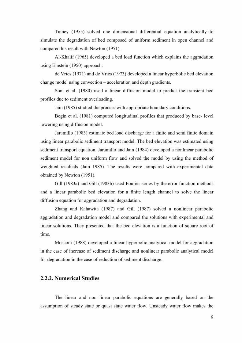
Sediment particles in water, might behave as a carrier for heavy metals which

have affinity to attach to cohesive sediments. They serve as the major pollutant and can

cause disruption of ecosystems. Sediment particles such as nitrogen, organic

compounds, residues, pathogenic bacteria, pesticides and viruses are carried into a

reservoir, deteriorate water quality and cause different illness (World Meteorological

Organization 2003).

Sedimentation and soil erosion are the modern world’s environmental topics.

These subjects have been studied for centuries by engineers. There are different

approaches for solving engineering problems. Sediment deposition deals with water and

sediment particles so, the physical properties of water and sediment particles should be

studied to understand sediment transport mechanism. Sediments are transported as

suspended and bed load as shown in Figure 1.1 depending upon fundamental properties

of water and sediment particle size, density, etc.

In a river system, loose surface can erode from basin by water and be transported

by stream. Sediment particles can be transported in four modes rolling, sliding, saltation

and suspension. While sediment particles are sliding and rolling, particles continue to be

at contact with the bed. Saltation means that jumping motion along the bed in a series of

low trajectories. Rolling and sliding particles move along the bed surface under the

force of the overlying flow of water. It is often unimportant to distinguish saltation from

rolling or sliding because saltation is restricted to only a few grain diameters in height

(Dyer 1986). A saltating grain may only momentarily leave the bed and rise no higher

than a few (<4) grain diameters. These three modes are bed load transport. Sometimes

sediments stay in suspension for an appreciable length of time called suspended load

transport. Suspension of a sediment grain is one of the modes in water systems that

occurs when the magnitude of the vertical component of the turbulent velocity is greater

than the settling speed of the grain. Bagnold (1966) argued that the major distinction in

sediment transport modes is between suspended and unsuspended (bed load) transport.

Bed load sediment grains and aggregates are transported under the combined processes

of saltation, rolling, and sliding, and receive insufficient hydrodynamic impulses to

overcome gravitational settling. Their only significant upward impulse is derived from

successive contacts with the bed (Dyer 1986). When the flow conditions satisfy or

exceed the criteria for incipient motion, sediment particles along an alluvial bed will

start to move (Yang 1996).

3

Figure 1.1. Different modes of sediment transport

(Source: Singh 2005)

It is essential to predict effects of sedimentation and loss of storage capacity in

advance for better operation of the reservoirs. Current research on reservoir

sedimentation prediction is mainly based on numerical modeling of sediment transport

methodologies (Hotchkiss and Parker 1991) and investigation of transport parameters in

the laboratory (Guy, et. al. 1966, Soni 1981a).

Free-surface flows can be classified into various types using criteria of their

classification (Chaudhry 1993). Steady and unsteady flows based on changes with

respect to time. In steady flow regimes, depth and velocity do not vary with time. If

depth and velocity at a point vary with time, the flow regime is classified as unsteady. It

is possible to transform an unsteady flow into a steady flow by having coordinates with

respect a moving reference in some cases. Studying steady flow is easier than unsteady

flows in governing mathematical models although the real world situation is unsteady

flow. Such a transformation is possible only if the wave shape does not change as the

wave propagates.

One of the other classifications based on changes with respect to space. If the

flow velocity at a given instant of time does not change within a given length of

channel, it is uniform flow. It means that the convective acceleration is zero. If the flow

velocity at a time varies with respect to distance, it is non-uniform flow. Steady and

4

unsteady flows are characterized by the variation with respect to time at a given

location, whereas the uniform and nonuniform flows are characterized by the variation

at a given instant of time with respect to distance.

The flow can be classified based on Reynolds number. If the liquid particles

appear to move in definite smooth paths and the flow appears to be as a movement of

thin layers on top each other, it is laminar flow. In natural channels, in laminar flow

Reynolds number is low than 500 ( )500Re < . The flow is characterized by the irregular

movement of particles of the fluid in turbulent flow, Reynolds number is greater than

600 ( )600Re < . If the flow is that 600Re500 << it is called transient flow.

The other classification is based on Froude number. The Froude Number is a

dimensionless parameter measuring of the ratio of the inertia force on an element of

fluid to the weight of the fluid element - the inertial force divided by gravitational force.

If the flow velocity is equal to celerity, it is critical flow ( )1=rF . If the flow velocity is

less than the critical velocity, it is subcritical flow ( )1<rF . If the flow is supercritical

the flow velocity is greater than the critical velocity ( )1>rF .

Hydraulic engineers generally treat channel in one dimension (1D). 1D flow

means that the longitudinal acceleration is significant, whereas transverse and vertical

accelerations are negligible.

Modeling of sediment transport can be assumed in equilibrium or non

equilibrium conditions. If detachment rate and deposition rate are equal, the flow is in

equilibrium condition. In non equilibrium condition, there is difference between

detachment rate and deposition rate. There is no doubt that natural rivers are mostly in

non equilibrium state. Because the real river systems behave as unsteady flow in non

equilibrium state, treating the system with steady flow in equilibrium state is a

simplification.

The main objective of this study is to develop unsteady and non equilibrium one

dimensional numerical model for sediment transport in rivers. For that aim, first of all

three numerical models were developed using the kinematic wave, diffusion wave and

dynamic wave, for describing the bed profile evolution and movement in alluvial

channels under equilibrium conditions. The models were evaluated by simulating bed

profiles for several hypothetical scenarios. The scenarios involve solving the equations

with different formulations of particle velocity, particle fall velocity, sediment flux and

5

different values of maximum bed elevation. Also, the models tested against measured

flume data and the solutions were compared.

This thesis includes six chapters. Chapter 1 aims to present a brief introductory

background to the research subject. Previous relevant physical and mathematical studies

are reviewed in Chapter 2. Sediment transport formulations are summarized in Chapter

3. The one dimensional hydrodynamic model is described by the governing equations in

Chapter 4. In Chapter 5, one dimensional sediment transport equations are governed in

two categories: equilibrium and nonequilibrium. Also three different wave approaches

were discussed: kinematic, diffusion and dynamic waves. The boundary conditions of

the numerical model used in the study, and the testing of the model are described.

Finally, in Chapter 6, the main results and the conclusions of the study are summarized.

6

CHAPTER 2

LITERATURE REVIEW

Sediment related disasters such as debris flow, landslides and slope collapses are

known to occur naturally, causing social and economically problems in the world.

Hence, the human civilizations study sediment transport to reduce the damages of the

disasters and to maximize the benefits of the water resources structures. The studies of

the sediment transport can be classified in two categories. Physical studies are related to

extensive flume and field observations. Mathematical studies are related to develop

theoretical and numerical methods.

2.1. Physical Studies

Physical studies are done by doing experiments in laboratory flumes or by taking

field observations. It is difficult to represent a river by a laboratory flume; so many

assumptions are usually incorporated in laboratory studies. The laboratory studies are

still important for understanding of basic concepts of river flow and sediment transport.

Many investigators have developed empirical methods to represent sediment transport

phenomena using data obtained in laboratory.

Taking real time observations are better to understand the complex real life river

systems. However it is very difficult to take real time data in the field and sometimes it

is even impossible.

Experimental studies have been mostly done with laboratory flume experiments

(Guy, et al. 1966, Langbein and Leopold 1968, Soni 1981a, Wathen and Hoey 1998,

Lisle, et al. 1997, Lisle, et al. 2001). Also laboratory studies are easier than field

measurements and provide control to particular combinations of initial and boundary

conditions (Curran and Wilcock 2005).

Newton (1951) studied, with a series experiments, degradation with uniform

sediment size. He saw that the bed elevation and bed slope decreased asymptotically

with time.

Leopold and Maddock (1953) obtained field data showing the relationship

between total sediment discharge and water discharge.

7

Lane and Borland (1954) conducted experiments to study riverbed scour during

floods. Laboratory data were obtained for degradation in alluvial channels by

Suryanarayana (1969).

Colby and Hembree (1955) compared the results of total sediment discharge and

water discharge between computed and measured from the Niobrara River near Cody,

Nebraska. Yang (1973) unit stream power equation gave the best agreement with those

measurements.

Bhamidipaty et al. (1971) studied with Newton’s analysis and combined their

own extensive laboratory flume studies for three different particle sizes with uniform

sediment grain sizes. They observed that the bed elevation in a degrading channel

decreases exponentially with time. Soni et al. (1980) conducted a similar experiment

using mobile bed under equilibrium conditions before the aggradation started. Hence

they formed experiment conditions to better present the real river systems and

developed a mathematical model for aggradation in an infinitely long channel. In 1980

Mehta (1980) improved studies by Soni et al. (1980) research with different sediment

size particles.

Vanoni (1971) compared the computed sediment discharges from different

equations with the measured results from natural rivers. Yang and Stall (1976) and

Yang (1977) reported his comparisons.

For aggradation and deggradation of non uniform sediments, Little and Mayer

(1972) conducted a series of experiments. They studied the variations of sediment

gradation on the bed surface during the armoring.

Ribberink (1985) studied the vertical sorting phenomenon of sediment having an

idealized gradation under the equilibrium conditions. He also proposed a transport layer

concept.

Yen et al. (1985) and Yen et al. (1988a) conducted a series of overloading

experiments using uniform coarse sediment and found that the mean sediment transport

velocity and aggradation wave speed increase with the initial equilibrium bed slope and

decrease with loading ration.

Wilcock and Southard (1989) did careful measurements and observations in

equilibrium conditions and investigated the interaction between the transport, bed

surface texture and bed configuration. Also, Wilcock et al. (2001) conducted five

different sediments in a laboratory flume by carrying out 48 sets of experiments of flow,

transport and bed grain size.

8

Yen et al. (1992) also did flume studies with constant median sediment particle

diameter but varying geometric standard deviation, so that the effect of non uniformity

in rivers could be taken into account. They investigated that aggradation and

degradation depends on materials vary so that the effect of non uniformity in rivers

could be taken into account.

Tang and Knight (2006) investigated the effect of flood plain roughness on bed

form geometry, bed load transport and dune migration rate.

Experimental flume studies have the limitations due to the complexity of

representing a real life river conditions. However, it helps us to understand basic

concepts of river flow and it provides a detailed analysis for parameters related to

physics of the problem.

2.2. Mathematical Studies

Both experimental flume studies and field observations have limitations in

predicting sediment transport capacity. Laboratory studies do not represent real life

river conditions, besides taking the survey data sometimes impossible. Due to these

restrictions, investigators have made many assumptions during the research. To study

the sediment transport mechanism, many investigators developed mathematical

equations for real life situations. All the sediment transport mathematical models

developed so far are based on five basic physical equations. These equations have been

developed by many researches that can be solved both analytically and numerically.

Solving the complex differential equations, numerical solutions are more

appropriate than analytical solutions. On the other hand analytical solutions can be

developed and applied only in very simplified and simple cases.

2.2.1. Analytical Studies

When flow conditions are very simplified in one dimensional case analytical

solution can be developed. Developing the solution is very complex for generalized two

or three dimensional cases with complex conditions. Some of the well known analytical

sediment models are summarized below.

9

Tinney (1955) solved one dimensional differential equation analytically to

simulate the degradation of bed composed of uniform sediment in open channel and

compared his result with Newton (1951).

Al-Khalif (1965) developed a bed load function which explains the aggradation

using Einstein (1950) approach.

de Vries (1971) and de Vries (1973) developed a linear hyperbolic bed elevation

change model using convection – acceleration and depth gradients.

Soni et al. (1980) used a linear diffusion model to predict the transient bed

profiles due to sediment overloading.

Jain (1985) studied the process with appropriate boundary conditions.

Begin et al. (1981) computed longitudinal profiles that produced by base- level

lowering using diffusion model.

Jaramillo (1983) estimate bed load discharge for a finite and semi finite domain

using linear parabolic sediment transport model. The bed elevation was estimated using

sediment transport equation. Jaramillo and Jain (1984) developed a nonlinear parabolic

sediment model for non uniform flow and solved the model by using the method of

weighted residuals (Jain 1985). The results were compared with experimental data

obtained by Newton (1951).

Gill (1983a) and Gill (1983b) used Fourier series by the error function methods

and a linear parabolic bed elevation for a finite length channel to solve the linear

diffusion equation for aggradation and degradation.

Zhang and Kahawita (1987) and Gill (1987) solved a nonlinear parabolic

aggradation and degradation model and compared the solutions with experimental and

linear solutions. They presented that the bed elevation is a function of square root of

time.

Mosconi (1988) developed a linear hyperbolic analytical model for aggradation

in the case of increase of sediment discharge and nonlinear parabolic analytical model

for degradation in the case of reduction of sediment discharge.

2.2.2. Numerical Studies

The linear and non linear parabolic equations are generally based on the

assumption of steady state or quasi state water flow. Unsteady water flow makes the

10

system complex and analytical solution is difficult to develop for the complex systems.

Numerical sediment transport models have been developed in one, two or three

dimensional have been listed below.

Lyn and Altinakar (2002) predicted bed elevation using quasi – steady model.

Curran and Wilcock (2005) studied constant flow rate and flow depth while

varying the sand supply.

Mathematical sediment transport models have been based on generally diffusion

wave and dynamic wave to predict bed profiles in alluvial channels. Whereas many

researchers (de Vries 1973, Soni 1981b, Soni 1981c, Ribberink and Van Der Sande

1985, Lisle, et al. 2001) studied diffusion equations, others (Ching and Cheng 1964,

Vreugdenhil and de Vries 1973, de Vries 1975, Ribberink and Van Der Sande 1985,

Pianese 1994, Lyn and Altinakar 2002, Cao and Carling 2003, Singh, et al. 2004,

Mohammadian, et al. 2004, Li and Millar 2007) studied dynamic equations. The

sediment transport function has been expressed as a function of water flow variables

and the bed formation and the bed movement has been treated as having diffusion

characteristics in literature (Tayfur and Singh 2006). On the other hand the experimental

studies by Langbein and Leopold (1968) provided that movement of bed profiles

behaves as kinematic wave, a function of sediment transport rate and concentration.

Kinematic wave theory applicatibility to unsteady flow routing problems is discussed by

Tsai (2003). Tayfur and Singh (2006) used the kinematic wave theory under equilibrium

conditions and modeled transient bed profiles.

Other mathematical approaches are equilibrium and nonequilibrium sediment

transport models. In equilibrium models, the actual sediment transport rate is assumed

to be equal to the sediment transport capacity at every cross section whereas in many

cases the inflow sediment discharge imposed at the inlet is different than the transport

capacity which might lead to difficulties in the calculation of bed changes near the inlet,

thus solved by non- equilibrium models. Calculation of the equilibrium models are

easier than non- equilibrium models. In many studies it was assumed that detachment

rate and deposition rate are equal. This assumption may be valid only if conditions such

as channel geometry, water and sediment properties are constant for a long period of

time. Natural rivers are mostly in non – equilibrium state. Wu et al. (2004) developed

one dimensional numerical model in unsteady flows under non – equilibrium

conditions. Tayfur and Singh (2007) developed a mathematical model using kinematic

wave theory under non – equilibrium conditions in alluvial rivers.

11

2.2.2.1. One Dimensional Model Studies

In rivers, the accelerations in lateral and vertical directions are mostly assumed

negligible and therefore, acceleration in longitudinal direction is generally utilized in

one dimensional models. This assumption simplifies the solution as it involves few

equations only in one direction. These models have been mostly solved based on finite

difference method to obtain bed elevation and water surface profiles (Perdreau and

Cunge 1971, Cunge and Perdreau 1973, Chang 1982, Krishnappan 1985, Rahuel, et al.

1989, Holly and Rahuel 1990a, Holly and Rahuel 1990b, Correia, et al. 1992, Holly, et

al. 1993).

de Vries (1965) has developed one dimensional model using explicit finite

difference scheme to compute bed and water elevation profiles.

Cunge et al. (1980) has developed one dimensional model simulations of alluvial

hydraulics.

Rahuel et al. (1989) studied unsteady flow models and have applied in river

conditions. Cui et al. (1996), Kassem and Chaudhry (1998), Cao and Egiashira (1999),

Capart (2000), Cao et al. (2001), Capart and Young (2002) and Di Cristo et al. (2002)

have studied similar models in resent years, wary numerical models.

The majority of one dimensional unsteady models can be divided into two

categories in the literature: (1)uncoupled flow models that water flow equations and

sediment continuity equation are solved separately and (2)quasi-steady flow models that

energy equation solved with sediment continuity equation. Only a few models are

coupled in literature. Lyn and Goodwin (1987) presented an approach to model fully

coupled unsteady water flow equations and sediment continuity equation. They

compared the solutions between stability of coupled and uncoupled models and

concluded that the coupled model is more stable. Other one dimensional coupled

sediment transport models presented by Rahuel and Holly (1989), Holly and Rahuel

(1990a, 1990b) simulating process between bed load and suspended load. Correria et al.

(1992), studied with full explicit coupling models using water continuity equation, so it

gives the permission to change the bed roughness depending on flow regime.

Bhallamudi and Chaudhry (1989) have presented one dimensional, unsteady and

coupled deformable bed model using Mac Cormack second order accurate explicit

scheme. They compared the results with experimental laboratory flumes data and saw

12

that the results are satisfactory. Singh et al. (2004) have developed a fully coupled one

dimensional alluvial river model and governed system of partial differential equations

using Preissmann finite difference scheme. The tests presented by simulating the Quail

Creek failure in Washington, USA. Wu et al. (2005) proposed one dimensional model

simulates under unsteady flow conditions in dendritic channel networks with hydraulic

structures. The equations solved in a coupling model and tested in several cases.

Although in uncoupled models, there is strong interaction between solid and

water phases of the flow, only the flow continuity and momentum equations are solved

simultaneously (Singh, et al. 2004). Park and Jain (1986) used Preissmann linearized

implicit scheme for simulating the governing equations in unsteady and uncoupled

models. Lyn (1987) studied uncoupled models and suggested that complete coupling

between the full unsteady flow equations and sediment continuity equation is desirable

in cases where the conditions change rapidly at the boundaries.

2.2.2.2. Two Dimensional Model Studies

Sediment concentration is averaged only along one direction, generally vertical

direction (depth – integrated) where vertical variations are not significant depending on

the flow characteristics in two dimensional models. One of the advantages of the 2D

simulation of flow and sediment transport is depth – averaged subsystem for river flow.

In depth – averaged models, all the model parameters are assumed to be same

everywhere the water column. The depth - integrated equations of motion and

continuity are linked to a depth - integrated sediment transport model (Boer, et al. 1984,

McAnally, et al. 1991). The two dimensional models are more difficult than the one

dimensional models and they provide more information about flow conditions.

Although the best mathematical model is the three dimensional it is not practical

since it requires much more computational time especially in longer river stretches. In

addition, enough experimental data cannot be available in general for model calibration.

Struiksma (1985) and Shimizu and Itakura (1989) developed a two dimensional

model for the simulation of the large scale bed change in alluvial channels.

Mohapatra and Bhallamudi (1994) developed two dimensional model using a

false transient principle with the quasi – steady uncoupled approach in a transformed

coordinate system and McCormack scheme was used for the numerical solution.

13

Chaudhary (1996) developed the model for straight and meandering channels.

MIKE21 (DHI 2003), TABS-MD (Thomas and McAnally 1990), CCHE2D (Wu

2001) and HSCTM2D (Hayter 1995) are the widely used two dimensional sediment

transport models.

MIKE21C is the curvilinear finite difference model. It has been developed at the

Danish Hydraulic Institute (DHI) for river morphology (Langendoen 1996). The effects

of secondary flow are taken into account by introducing quasi – steady approach in

curved channels. In bends, the direction of sediment transport has been determined by

using this secondary flow. Also, the model has been used to simulate critical

morphological and hydrodynamic conditions.

One of the depth – integrated two dimensional sediment transport model is

CCHE2D (Wu 2001). This model is based on variantion of the finite element method

using depth – average ε−k models to estimate the turbulent eddy viscosity. The

secondary flow effects were modeled on bed load direction in curved channels although

fluid momentum and sediment transport rate effects were not. This model is applicable

for morphological problems in rivers.

HSCTM2D (Hydrodynamic, Sediment and Contaminant Transport Model)

model was developed for U. S. Environmental Protection Agency which based on the

finite element method and vertically integrated in cohesive sediments.

Other well known models for simulation of sediment transport are TRIM-2D

(Casulli 1990) based on finite difference approach and was adapted for practical

applications. MOBED2 (Spasojevic and Holly 1990) models with finite difference and

applicable in natural rivers, and TELEMAC2D with its module TSEF based on standard

equilibrium bed load formulations as Meyer – Peter Müller (1948) uses ε−k models

with finite element model.

Minh Duc et al. (2004) developed a depth – averaged model using a finite

volume method to calculate bed deformation in alluvial channels.

Li and Millar (2007) studied two dimensional hydrodynamic bed model to

simulate bed load transport.

14

2.2.2.3. Three Dimensional Model Studies

The sediment transport process in alluvial channels could be described best by

three dimensional models that include all the space dimensions. Since the full equations

of motion are solved, the model is the most complicated and resource consuming in

implementation. When the flow is stratified in salinity or temperature, mostly three

dimensional models are applicable.

Demuren and Rodi (1986) used ε−k models to develop neutral tracer transport

model.

Wan and Adeff (1986) developed finite element method for unsteady flow.

Van Rijn (1987) developed equations for mass balance using three dimensional

equations and combined them with two dimensional depth integrated model.

Lin and Falconer (1996) developed a three dimensional sediment transport

model for estuaries and coasts.

Hamrick (1996) developed EFDC and tested numerical model. EFDC can

simulate flow processes in all three dimensions in rivers, lakes, reservoirs, estuaries,

wetlands and coastal regions.

Wu (2000) studied three dimensional models for straight channels.

Delft-3D (Delft Hydraulics 2002) and ECOMSED (HydroQual Inc. 2003) are

general three dimensional models that are used widely.

ECOMSED is the sediment transport model that was developed by HydroQual,

Inc. and Delft Hydraulics (Blumberg and Mellor 1987) for estuaries and oceans. This

model is applicable only up to a diameter size of 500 mμ and cannot be applied for bed

load transport. HydroQual, Inc. developed the SED module of ECOMSED (2002). A

three dimensional suspended sediment transport model is SED formed for non cohesive

sediments using implicit scheme.

2.3. Measurement Surveys

The geomorphologic data of river can be obtained by a topographic survey,

including a land survey and groundwater surveying, or by repetitive surveying with pre-

determined ranges, since samples size distribution can be found and determined the dry

density or unit weight. Also, surveying of reservoirs are required to determine

15

sedimentation rates and to assess overall capacity of the reservoir. For surveying,

manual sounding poles, sounding weights and echo sounders are commonly used. For

reasons of economy, accuracy and expediency, sedimentation surveys were carried out

in small reservoirs or cross small river reaches. More advanced instruments have been

adopted as electronic distance measuring systems for large reservoirs. Sedimentation

surveys are best reliable for the accurate positioning of measuring points where no

deposition or erosion takes place, the elevation of the bed surface should coincide with

that measured in a previous survey (Bor, et al. 2008). This is a good check of the

accuracy and reliability of the sedimentation surveys. In addition to this detailed

bathymetry map, thickness and long-term average accumulation rates of the lake can be

determined by using echo sounder systems (Odhiambo and Boss 2004). Other studies in

literature about surveying using acoustic methods include the technical details of

scanning (Urick 1983), techniques used for sediment mapping (Higginbottom, et al.

1994), and the comparison of different echoes on sediment type (Collins and Gregory

1996).

Also, in hydrometric stations for sediment measurement, suspended sediment

discharge and sediment concentration, size gradation of suspended sediment and bed

material can be measured the whole year around.

Taking real time observations can explain the real life systems better than flume

experiments but it is very difficult to take real time data in the field even sometimes it is

impossible.

16

CHAPTER 3

MECHANICS OF SEDIMENT TRANSPORT

Sediment transport mechanism is concerned about water and sediment particles.

An understanding of the sediment transport mechanism requires the learning of the

physical properties of water and sediment particles. Fundamental properties of water

and sediment particles are described below.

3.1. Physical Properties of Water

The fundamental properties of water are important in sediment transport studies.

They are summarized below.

3.1.1. Specific Weight

Specific weight is defined as weight per unit volume. Specific weight can be

expressed as (Yang 1996):

gργ = (3.1)

where,

γ =specific weight (M/L2/T2)

ρ =density (M/L3)

g =gravitational acceleration (L/T2)

3.1.2. Density

Quantity of matter contained in a unit volume of the substance.

=ρ vm / (3.2)

17

where,

m =mass (M)

v =volume (L3)

3.1.3. Viscosity

Due to cohesion and interaction between molecules, resistance to deformation is

observed. Viscosity of the property defines the rate of this resistance to deformation.

Newton’s law of viscosity relates shear stress and velocity gradient by dynamic

viscosity.

dyduμτ = (3.3)

where,

τ =shear stress (M/L2)

μ =dynamic viscosity (M / (LT))

dydu

=velocity gradient

Kinematic viscosity is the ratio between dynamic viscosity and fluid density

(Yang 1996).

ρμυ = (3.4)

where,

υ =kinematic viscosity (L2/T)

The properties of water are summarized in Table 3.1.

3.2. Physical Properties of Sediment

Particle size, shape specific gravity and fall velocity are important for

understanding of sediment transport mechanism.

18

3.2.1. Size

Particle size clearly describes the physical properties of the sediment particle, so

it is the most important parameter for many practical purposes. The sediment size can

be measured by various methods such as sieve analysis, optical methods or visual

accumulation tube analysis. The sediment grade scale suggested by Lane (1947), as

shown in Table 3.1. It was adopted by American Geophysical Union and is still used by

hydraulic engineers.

Table 3.1. Properties of water

(Source: Yang 1996)

Temperature (0C)

Specific Weight

γ (kN/m3)

Density ρ (kg/m3)

Dynamic Viscosity

μ x 103 (N-s/m2)

Kinematic Viscosity

v x 10-6 (m2/s)

0 9.805 999.8 1.781 1.785 5 9.807 1000.0 1.518 1.519 10 9.804 999.7 1.307 1.306 15 9.798 999.1 1.139 1.139 20 9.789 998.2 1.002 1.003 25 9.777 997.0 0.890 0.893 30 9.764 995.7 0.798 0.800 40 9.730 992.2 0.653 0.658 50 9.689 988.0 0.547 0.553 60 9.642 983.2 0.466 0.474 70 9.589 977.8 0.404 0.413 80 9.530 971.8 0.354 0.364 90 9.466 965.3 0.315 0.326 100 9.399 958.4 0.282 0.294

3.2.2. Shape

Particle shape is the second most significant sediment property in natural

sediments. The geometric configuration defines shape parameter regardless of sediment

particle size and composition. Grains are usually considered to have with long diameter

19

a, intermediate diameter b and short diameter c. Corey (Schulz, et al. 1954) investigated

several shape factors and defined the shape factor as:

abcCSF = (3.5)

Corel shape factor was the most significant expression of shape. The shape

factor for a sphere would be 1.0. Natural sediment typically has a shape factor of about

0.7 (US Army Corps of Engineers 2008).

3.2.3. Particle Specific Gravity

Specific gravity is defined as the ratio of the specific weight of the sediment to

that of water. It usually ranges numerically from 2.6 to 2.8 in natural solids. While the

lower values of specific gravity are typical of the coarser soils, higher values are typical

of the fine – grained soil types. Due to its resistance to weathering and abrasion, quartz,

which has a specific gravity of 2.65, is the most common mineral found in natural

noncohesive sediments. Typically, the average specific gravity of a sediment mixture is

close to that of quartz. Therefore, in sedimentation studies, specific gravity is frequently

assumed to be 2.65, although whenever possible, site-specific particle specific gravity

should be determined (US Army Corps of Engineers 2008).

3.2.4. Fall Velocity

Fall velocity or settling velocity is the most fundamental property governing the

motion of the sediment particle in a fluid. It is a function of the volume, shape and

density of the particle and the viscosity and density of the fluid. The fall velocity of any

naturally worn sediment particle may be calculated if the characteristics of the particle

and fluid are known. Fall velocity is related to relative flow conditions between the

sediment particle and water during conditions of sediment entrainment, transportation

and deposition. Fall velocity can be calculated from a balance between the particle

buoyant weight or submerged weight and the resulting force from fluid drag (Yang

1996). The general drag equation is

20

2

2f

DD

vACF ρ= (3.6)

where,

DF = drag force

DC = drag coefficient

ρ = density of water

A = the projected area of particle in the direction of fall

fv = the fall velocity

The particle buoyant weight or submerged weight of a spherical sediment

particle is

grW ss )(34 3 ρρπ −= (3.7)

where,

sW =submerged weight

r =particle radius

sρ and ρ = densities of sediment and water respectively.

For very slow, steady moving sphere, the drag coefficient thus obtained is

Re24

=DC (3.8)

This equation is acceptable for Reynolds numbers less than 1.0 where;

υ

sf dv=Re (3.9)

where,

υ = kinematic viscosity of water

sd =sediment diameter

From Equation 3.6 and Equation 3.8, Stokes (1851) equation can be obtained;

21

υρπ fD vdF 3= (3.10)

Equality of Equation 3.7 and Equation 3.10, the fall velocity for a sediment

particle can be obtained as below:

υγ

γγ 2

181 s

w

wsf

dgv −= (3.11)

where,

sγ and wγ = specific weights of sediment and water respectively.

This equation is acceptable for the particle diameter equal to or less than 0.1

mm.

The drag coefficient of a sphere depends on the Reynolds number. When the

particle Reynolds number is greater than 2.0, the particle fall velocity is determined

experimentally. Rouse (1937) gave smv f /024.0= for most natural sands, the shape

factor is 0.7 and mmds 2.0= .

There are many approaches about fall velocity in literature. Some of them

summarized below:

3.2.4.1. Dietrich Approach

Dietrich (1982) developed the following equation for fall velocity analyzing

empirical relation.

)(3*

2110 RRRW += (3.12)

where,

*W = the dimensionless fall velocity

υρρρ

gv

Ws

f

)(

3

* −= (3.13)

22

4

*

3*

2**1

)(log00056.0

)(log00575.0)(log0982.0)(log929.1767.3

D

DDDR

+

−−+−= (3.14)

)6.4(log)1)(5.0(3.0

]6.4tanh[log)1(85.0

)1(1log

*2

*3.2

2

−−−+

−−−⎥⎦⎤

⎢⎣⎡ −−=

DCSFCSF

DCSFCSFR (3.15)

⎥⎦⎤

⎢⎣⎡ −+

⎥⎦

⎤⎢⎣

⎡⎟⎠⎞

⎜⎝⎛ −−=

5.2)5.3(1

*3 ]6.4tanh[log83.2

65.0

P

DCSFR (3.16)

where,

*D = the dimensionless particle size

CSF = the Corey shape factor

The dimensionless particle size *D is expressed as (Dietrich 1982):

2

3

*)(

ρυρρ ss gd

D−

= (3.17)

The Corey shape factor (CSF) is expressed as (Dietrich 1982):

5.0)(abcCSF = (3.18)

where,

a,b,c= the longest intermediate and shortest axes of the particle respectively and

mutually perpendicular.

* 8.05.0 −≈CSF (Dietrich 1982)

P = Powers value of roughness ( P is between 3.5 and 6 (Dietrich 1982))

23

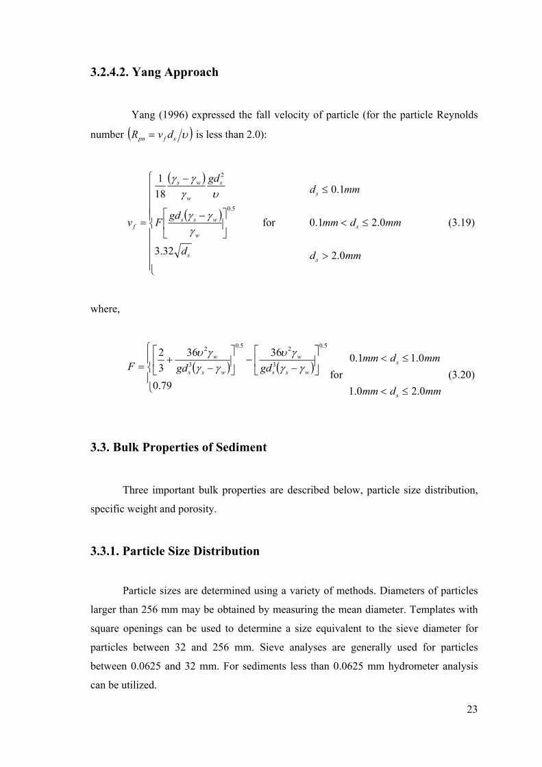
3.2.4.2. Yang Approach

Yang (1996) expressed the fall velocity of particle (for the particle Reynolds

number ( )υsfpn dvR = is less than 2.0):

( )

( )

⎪⎪⎪⎪

⎩

⎪⎪⎪⎪

⎨

⎧

⎥⎦

⎤⎢⎣

⎡ −

−

=

s

w

wss

s

w

ws

f

d

gdF

gd

v

32.3

181

5.0

2

γγγ

υγγγ

for

mmd

mmdmm

mmd

s

s

s

0.2

0.21.0

1.0

>

≤<

≤

(3.19)

where,

( ) ( )⎪⎩

⎪⎨

⎧⎥⎦

⎤⎢⎣

⎡−

−⎥⎦

⎤⎢⎣

⎡−

+=

79.0

363632

5.0

3

25.0

3

2

wss

w

wss

w

gdgdF γγγυ

γγγυ

for mmdmm

mmdmm

s

s

0.20.1

0.11.0

≤<

≤< (3.20)

3.3. Bulk Properties of Sediment

Three important bulk properties are described below, particle size distribution,

specific weight and porosity.

3.3.1. Particle Size Distribution

Particle sizes are determined using a variety of methods. Diameters of particles

larger than 256 mm may be obtained by measuring the mean diameter. Templates with

square openings can be used to determine a size equivalent to the sieve diameter for

particles between 32 and 256 mm. Sieve analyses are generally used for particles

between 0.0625 and 32 mm. For sediments less than 0.0625 mm hydrometer analysis

can be utilized.

24

The variation in particle sizes in a sediment mixture is described with a

gradation curve, which is a cumulative size-frequency distribution curve showing

particle size versus accumulated percent finer, by weight. It is common to refer to

particle sizes according to their position on the gradation curve. d50 is the geometric

mean particle size; that is, 50 percent of the sample is finer, by weight; d84.1 is 1

standard deviation larger than the geometric mean size in practice and it is rounded to

d84, while d15.9 is 1 standard deviation smaller then the geometric mean size and it is

rounded to d16 in practice (US Army Corps of Engineers 2008).

3.3.2. Specific Weight

Specific weight of deposited sediment is the weight per unit volume. It is

expressed as dry weight.

wd SGp γγ )1( −= (3.21)

or

sd p γγ )1( −= (3.22)

where,

dγ = specific weight of deposited sediment

SG = specific gravity of sediment particle

p =porosity

Specific weight increases with time after initial deposition. It also depends on

the composition of the sediment mixture (US Army Corps of Engineers 2008).

3.3.3. Porosity

It is defined as the ratio of volume of voids to total volume of sample. Porosity is

affected by particle size, shape and degree of compaction.

25

t

v

VV

p = (3.23)

where,

vV =void volume

tV =total volume of sample

3.4. Incipient Motion Criteria

The concept of incipient motion of sediment particles from the bed is important

to understand the aggradation and degradation forces acting on a spherical sediment

particle shown in Figure 3.1. The component of gravitational force in the direction of

flow can be neglected compared to other forces acting on a spherical sediment particle

because the channel slopes are small enough in most natural rivers. Other forces are

drag force DF , lift force LF , submerged weight SW and resistance force RF . A sediment

particle starts the incipient motion when the conditions are satisfied below (Yang 1996).

Figure 3.1. Settling of sphere in still water

(Source: Yang 1996)

where,

RO

RD

SL

MMFFWF

===

26

OM =overturning moment due to DF and RF

RM =resisting moment due to LF and SW

Different researchers developed several approaches defining the incipient

motion of sediment particles.

3.4.1. Shear Stress Approach

In early 1936, Shields (1936) derived a function for incipient motion of sediment

particles where balance of forces acting on a particle on a bed was considered. He

applied dimensional analysis to determine dimensionless parameters and investigated

the relationship between these two parameters by experimental studies.

⎟⎠⎞

⎜⎝⎛=

− υγγτ s

sws

c dUfd

*

)( (3.24)

υsdU*Re = (3.25)

where,

Re =Reynolds number

*U = shear velocity

cτ = critical shear stress at initial motion

Vanoni (1975) developed diagram fitting the curve to the data provided by

Shields (Figure 3.2). Figure 3.2. shows the results of experiments about relationship

between dimensional shear stress and particle Reynolds number.

Shields simplified the problem by neglecting the lift force and considered only

the drag force. The American Society of Civil Engineers Task Committee on the

Preparation of Sediment Manual modified diagram and uses a third parameter as shown

in Figure 3.2. The parameter is

2/1

11.0⎥⎥⎦

⎤

⎢⎢⎣

⎡⎟⎟⎠

⎞⎜⎜⎝

⎛− s

w

ss gddγγ

υ (3.26)

27

This parameter allows determination of intersection with the Shields diagram

and its corresponding values of shear stress. Many investigators have proposed different

options which are more or less the same.

Figure 3.2. Shields diagram for incipient motion

(Source: Vanoni 1975)

3.4.2. Velocity Approach

Velocity approach uses the relationship between the velocity field and shear

stress field. It means that the velocity for incipient motion can be calculated if the drag

force for incipient motion is known.

Yang (1973) obtained incipient motion criteria using laboratory data collected

by different investigators. The relationship between dimensionless critical average flow

velocity and Reynolds number follows a hyperbola when the Reynolds number is less

than 70 summarized in Equation 3.27. When the Reynolds number greater than 70,

ω/crV becomes a constant, as shown Equation 3.28. (Singh 2005).

( ) ,06.006.0/log

5.2

*

+−

=vdUv

V

sf

cr 702.1 * <<υ

sdU (3.27)

,05.2=f

cr

vV

vdU s*70 ≤ (3.28)

28

3.4.3. Meyer – Peter and Müller Criterion

Meyer – Peter and Müller (1948) obtained bed load equation and sediment size

at incipient motion as formulated from bed load equation (Yang 1996).

( ) 2/36/1901 / dnK

SDds = (3.29)

where,

sd =sediment size in the armor layer (in mm)

S =channel slope

D =mean flow depth

1K =constant (=0.9 when D is in ft and 0.058 when D is in m)

n =channel bottom roughness or Manning’s roughness coefficient

90d =bed material size where 90% of the material is finer (in m)

3.5. Resistance to Flow with Rigid Boundary

Prandtl’s (1926) mixing theory depends on velocity distribution approach.

Velocity at distance y is

*log75.55.8 Ukyus⎟⎟⎠

⎞⎜⎜⎝

⎛+= (3.30)

and

**log75.55.5 UyUu ⎟⎠⎞

⎜⎝⎛ +=

υ (3.31)

where,

u =velocity at a distance y above the bed

gDSU =* =shear velocity

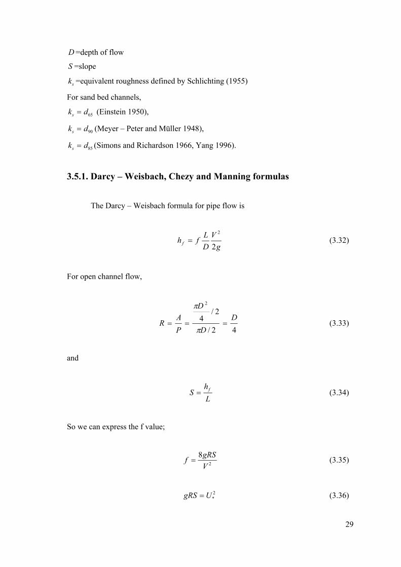
29

D =depth of flow

S =slope

sk =equivalent roughness defined by Schlichting (1955)

For sand bed channels,

65dks = (Einstein 1950),

90dks = (Meyer – Peter and Müller 1948),

85dks = (Simons and Richardson 1966, Yang 1996).

3.5.1. Darcy – Weisbach, Chezy and Manning formulas

The Darcy – Weisbach formula for pipe flow is

gV

DLfh f 2

2

= (3.32)

For open channel flow,

42/

2/4

2

DD

D

PA

R ===π

π

(3.33)

and

Lh

S f= (3.34)

So we can express the f value;

2

8VgRSf = (3.35)

2*UgRS = (3.36)

30

2/1

*

8⎟⎟⎠

⎞⎜⎜⎝

⎛=

fUV (3.37)

where,

fh =friction loss

f =Darcy – Weisbach friction factor

L =pipe length

D =pipe diameter

V =average flow velocity

R =hydraulic radius

S =energy slope

The Chezy formula is

RSCV z= (3.38)

Shear stress along the boundary is

20 8

1Vfρτ = (3.39)

From relationship between RU ,, *0τ and V , Chezy coefficient can be obtained by

2/1

8⎟⎟⎠

⎞⎜⎜⎝

⎛=

ργ

fCz (3.40)

The Manning formula is

2/13/21SR

nV = (3.41)

where,

n =Manning coefficient and can be obtained by the formula below;

31

1.21

6/1dn = (3.42)

where,

d =sediment diameter of uniform sand in m (Yang 1996).

3.6. Bed Forms

Rate of sediment transport mainly depends on resistance to flow and bed

configuration. Simons and Richardson (1960) summarized bed forms as shown in

Figure 3.3. below (Yang 1996).

Ripples begin to form, as current velocity picks up in lower flow regime. These

are small bed forms, generally wavelengths less than 30 cm and heights less than 5 cm.

In faster currents, ripples grow into dunes. Dunes are similar to bars but larger than

ripples. Their profile height is limited by depth of flow, so they can be several meters

tall in deep water. Bars are bed forms having lengths the same as channel width and

height same as channel height. In higher velocities dunes are destroyed and plane bed

forms occur. In very high velocities anti dune bed forms occurs. Water surface forms

waves that move upstream and so anti dunes move upstream. These are also called

standing waves. In large slopes, high velocities and sediment concentrations chutes and

pools occur. They consist of large elongated mounds of sediment. In transition zone,

bed configurations range from dunes to plane beds or to anti dunes.

32

Figure 3.3. Bed forms of sand bed channels

(Source: Simon and Richardson 1966)

3.7. Mechanism of Sediment Transport

Sediments are eroded from basin by water and transported by stream when the

flow conditions exceed the criteria for incipient motion. The motion can be rolling,

sliding or jumping along the bed which is called bed load transport. Sometimes

sediments stay in suspension for an appreciable length of time called suspended load

transport. In addition, wash load is a bed material load according the particle size and

mainly moves as suspended load. So, sediment can be classified as bed material load

and wash load or bed load and suspended load. Wash load transport is a function of

basin characteristics, whereas bed load transport is a function of flow characteristics

(Yang 1996) (Figure 3.4).

33

Figure 3.4. Movement types of sediment particles

3.7.1. Bed Load Transport Formulas

Bed load motion starts when critical conditions are exceed. The motion

concerned with two phase (solid + liquid) flow near the bed. Generally, the bed load

transport rate of a river is about 5-25% of that in suspension. Bed load measurement is

difficult, so it is estimated by sediment transport formulas based on different modes of

motion employing different parameters, including shear stress and flow velocity. The

approaches for prediction of bed load are briefly summarized as follows.

3.7.1.1. DuBoys Approach

Duboys (1879) developed a bed load model using shear stress approach. This

model consists of sediment particles moving in layers because of the tractive force

acting along at the bed. The bed load capacity formula is given as;

( )cb Kq τττ −= (3.43)

where; Straub (1935) defined K coefficient depending on the sediment particle

characteristics.

34

4/3

173.0d

K = (3.44)

Thus DuBoys equation can be rewritten as,

( )cs

b dq τττ −= 4/3

173.0 (3.45)

where,

sd =sediment particle diameter in mm

τ and cτ =bed and critical shear stress respectively in Ib/ft2

bq =bed load transport capacity in (ft3/sec)/ft

3.7.1.2. Meyer – Peter’s Approach

Meyer-Peter et al. (1934) developed the following bed load formula using the

energy slope approach in metric system;

174.0 3/23/2

−=ss

b

dSq

dq (3.46)

where,

bq =bed load [in (kg/s)/m]

q =water discharge [in (kg/s)/m]

S =Slope

sd =particle size (in m)

Meyer – Peter formula is valid only for coarse material sediment particle

diameters greater then 3 mm. For mixtures of non uniform material, d should be

replaced by 35d , where 35% of the mixture is finer than 35d (Yang 1996).

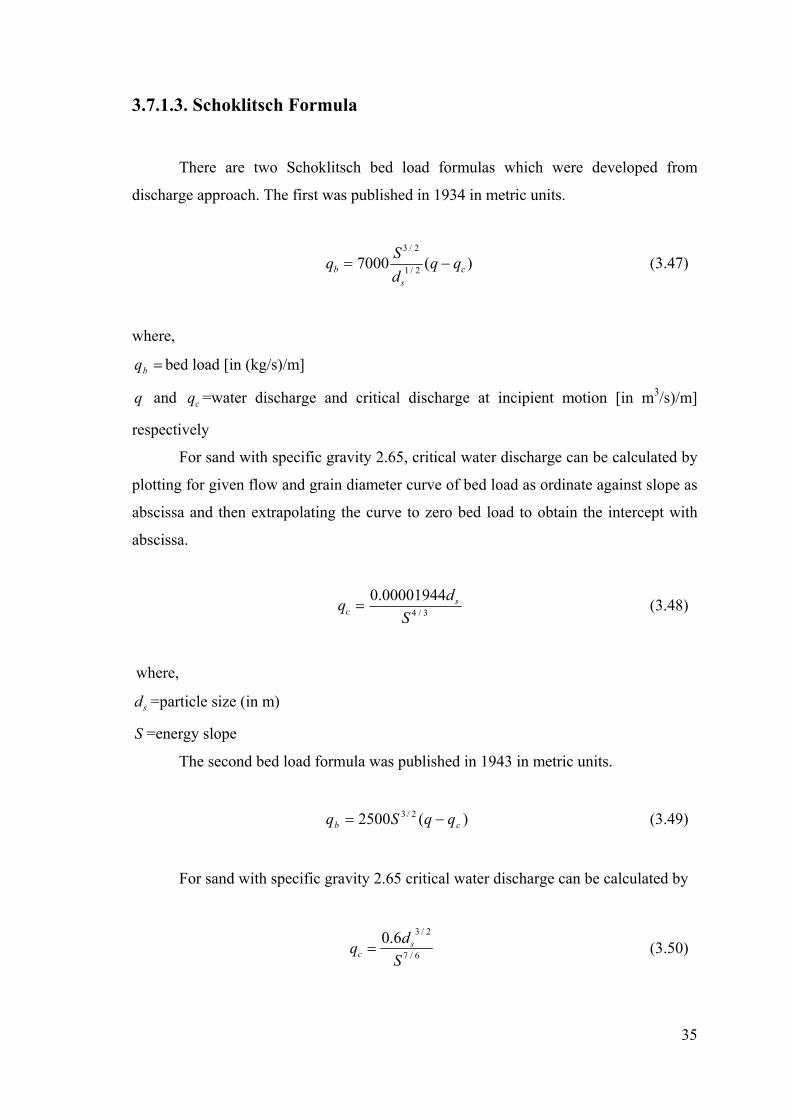
35

3.7.1.3. Schoklitsch Formula

There are two Schoklitsch bed load formulas which were developed from

discharge approach. The first was published in 1934 in metric units.

)(7000 2/1

2/3

cs

b qqdSq −= (3.47)

where,

=bq bed load [in (kg/s)/m]

q and cq =water discharge and critical discharge at incipient motion [in m3/s)/m]

respectively

For sand with specific gravity 2.65, critical water discharge can be calculated by

plotting for given flow and grain diameter curve of bed load as ordinate against slope as

abscissa and then extrapolating the curve to zero bed load to obtain the intercept with

abscissa.

3/4

00001944.0S

dq sc = (3.48)

where,

sd =particle size (in m)

S =energy slope

The second bed load formula was published in 1943 in metric units.

)(2500 2/3cb qqSq −= (3.49)

For sand with specific gravity 2.65 critical water discharge can be calculated by

6/7

2/36.0S

dq sc = (3.50)

36

3.7.1.4. Shields Approach

Shields (1936) conducted laboratory studies and obtained the flow conditions

corresponding to incipient motion when sediment transport greater than zero. Shield’s

measurements provided semi empirical equation for estimating bed load transport

capacity (with English units);

( ) sws

c

w

sb

dSqq

γγττ

γγ

−−

= 10 (3.51)

where,

bq and q =bed load and water discharge per unit channel width, respectively

DSγτ =

cτ can be obtained from Shields diagram (Yang 1996).

3.7.1.5. Meyer – Peter and Müller’s Approach

Meyer-Peter and Müller (1948) transformed the Meyer-Peter bed load formula

by isolating involved parameters one by one.

3/23/12/3 25.0)(047.0)( bwsr

s qdRSKK ργγγ +−= (3.52)

where,

R =hydraulic radius (in m)

S =energy slope

d =mean particle diameter (in m)

=ρ specific mass of water (in metric ton – s/m4)

=bq bed-load rate in underwater weight per unit time and width [in (metric ton / s)/m]

=SKK rs )/( the kind of slope which is adjusted for energy loss due to grain resistance

rS , is responsible for the bed-load motion.

Energy slope can be calculated by Strickler (1923) formula:

37

3/42

2

RKVSs

= (3.53)

Energy loss due to grain resistance can be calculated by Strickler’s formula as:

3/42

2

RKVSr

r = (3.54)

So;

2/1

⎟⎠⎞

⎜⎝⎛=

SS

KK r

r

s (3.55)

The formula is based on a large quantity of experimental data. Test results

showed the relationship to be of the form;

SS

KK r

r

s =⎟⎟⎠

⎞⎜⎜⎝

⎛2/3

(3.56)

And

6/190

26d

Kr = (3.57)

where,

=90d the size of sediment for which 90% of the material is finer (Yang 1996).

3.7.1.6. Regression Approach

Rottner (1959) expressed bed load discharge in terms of the flow parameters

based on regression analysis. The formula is dimensionally homogeneous (Yang 1996).

38

( )[ ]

( )[ ]

33/250

3/250

2/1

2/13

778.014.0667.01

1

⎪⎭

⎪⎬⎫

⎪⎩

⎪⎨⎧

⎟⎠⎞

⎜⎝⎛−

⎥⎥⎦

⎤

⎢⎢⎣

⎡+⎟

⎠⎞

⎜⎝⎛

−×

−=

Dd

Dd

gDV

gDq

s

ssb

ζ

ζγ

(3.58)

where,

bq =bed load discharge (in Ib/s per ft of width)

sγ =specific weight of sediment (in Ib/ft3)

sξ =specific gravity of the sediment (=2.65)

g =acceleration of gravity (in ft/s2)

D =mean depth (in ft)

V =mean velocity (in ft/s)

50d =particle size at which 50% of the bed material by weight is finer (in ft)

3.7.1.7. Chang, Simons and Richardson’s Approach

Chang, Simons and Richardson (1965) suggested that the bed load discharge by

weight can be determined using shear stress approach;

( )( ) φγγ

ττγtan−

−=

s

csbb

VKq (3.59)

( )ctb VKq ττ −= (3.60)

where,

bK =constant

tK =obtained by graph in English unit

φ =angle of repose of submerged material

bq =bed load transport capacity in Ib/ft/s (Yang 1996).

39

3.7.1.8. Parker et al. (1982) Approach

Parker et al. (1982) developed bed load transport formula using the hypothesis of

equal mobility.

ssi

bisi DgDp

qW 2/1

*

)()1/( −

=γγ

(3.61)

*

*

rττ

φ = (3.62)

*

*

ri

ii τ

τφ = (3.63)

*50

*50

50rτ

τφ = (3.64)

where,

=sD grain size

γ and =sγ specific weights of water and sediment

=biq bed-load per unit channel with in size fraction id

=ip friction by weight in size id

g=gravitational acceleration

=τ bed stress

sgDℜ= ρττ /* : Shields stress for grain size Ds

ii gDℜ= ρττ /* : Shields stress for i th grain size range

50*

50 / gDℜ= ρττ : Shields stress for median diameter of subpavement

=*rτ reference value of *τ at which **

rWW =

=*riτ reference value of i

*τ at which **ri WW =

=*50rτ 0.0876 reference value of *

50τ

40

Submerged=ℜ specific gravity of sediment

ρ = density of water

*)1/( riis

si d

Dτγγ

φ−

= (3.65)

The value of *riτ based on 50d is 0.0875

iri dd /0875.0 50* =τ (3.66)

[ ]25050

* )1(28.9)1(2.14exp0025.0 −−−= φφW , 0.95< 50φ <1.65 (3.67)

or

5.4

50

* 822.012.1 ⎟⎟⎠

⎞⎜⎜⎝

⎛−=

φW , 50φ >1.65 (3.68)

where,

=*iW dimensionless bed-load in i th grain size sub range

=*W dimensionless total bed-load

3.7.1.9. Tayfur and Singh’s Approach

Tayfur and Singh (2006) derived sediment flux equation from Langbein and

Leopold (1968) sediment flux concentration equation. Tayfur and Singh obtained

following equation from the kinematic wave theory approach.

⎥⎦

⎤⎢⎣

⎡−=

max

1z

zzpVq sbs (3.69)

41

where,

=bsq the sediment flux in movable bed layer (L2/T)

=sV the velocity of sediment particles as concentration approaches zero (L/T)

maxz =the maximum bed elevation

z = the mobile bed layer elevation

p = porosity of the bed layer

3.7.2. Suspended Load Transport Formulas

Settling velocities are balanced by upward component of turbulent velocity and

stays in suspension. While particles fall, some of them are carried away with high flow

velocity and then returning near the bed region. Others particles caught in an upward

moving eddy are lifted again. The higher the turbulence, the smaller the particle size

and the greater the portion of the particles is lifted up. Thus some sediment is kept in

suspension. Some basic suspended load formulas are summarized below.

3.7.2.1. The Rouse Equation

The downward transport rate is settling by gravity and the upward transport rate

is rising by diffusion must be balanced under steady equilibrium conditions. Settling by

gravity and the rising by diffusion components in opposite direction, respectively are

Cω and dydC

sε where;

ω =fall velocity of sediment particles

C =sediment concentration

dydC =concentration gradient

sε =momentum diffusion coefficient for sediment. It is function of y.

In the form of balance;

0=+dydCC sεω (3.70)

42

Assuming the mass transfer coefficient is equal to momentum transfer coefficient;

ms βεε = (3.71)

where,

mε =momentum transfer coefficient

β =a factor of proportionality

In turbulent flows, the turbulent shear stress is;

dydu

my ρετ = (3.72)

A distance y above the bed is

( ) ⎟⎠⎞

⎜⎝⎛ −=−=

hyyhSy 1τγτ (3.73)

Assuming logarithmic velocity distribution;

kyU

dydu *= (3.74)

where,

u =local velocity at a distance y above the bed

*U =shear velocity

k =Prandtl-von Karman universal constant

From the equations below, mε and sε can obtained:

⎟⎠⎞

⎜⎝⎛ −=

hyykUm 1*ε (3.75)

⎟⎠⎞

⎜⎝⎛ −=

hyykUs 1*βε (3.76)

43

To integration Equation 3.70 a to y by substituting sε ,

∫ ∫⎟⎠⎞

⎜⎝⎛ −

−=y

a

y

a

hyykU

dyCdC

1*β

ω (3.77)

For fine sediments β can be assumed 1,

( )∫ −−=

y

aa

dyyhykU

hCC

*

ln ω (3.78)

When α is equal to;

( )yhykU −=

*

ωα (3.79)

So;

The Rouse (1937) equation becomes

α

⎟⎟⎠

⎞⎜⎜⎝

⎛−

−=

aha

yyh

CC

a

(3.80)

3.7.2.2. Lane and Kalinske’s Approach

Lane and Kalinske (1941) assumed 1=β and obtained sediment concentration

in English units as;

⎟⎟⎠

⎞⎜⎜⎝

⎛=

hUa

PqCq Lasw*

15exp

ω (3.81)

44

where,

LP can be obtained by function of 6/1Dn and

*Uω with the results shown in Yang (1996)

book Figure 5.6.

3.7.2.3. Einstein’s Approach

Einstein (1950) replaced *U with '*U and assumed 1=β and obtained α as;

*4.0 Uω

α = (3.82)

Suspended load transported rate is

dycuqh

a∫= (3.83)

For any unit system

∫ ⎟⎠⎞

⎜⎝⎛

Δ⎟⎟⎠

⎞⎜⎜⎝

⎛−

−=

h

aa dyyU

aha

yyhCq 2.30log75.5 '

*

α

(3.84)

where,

xdxks // 65==Δ

Einstein (1950) obtain x and δ

sk that shown in Yang (1996) book Figure 3.9.

After substituting the logarithm velocity distribution formula simplifying one obtains:

⎥⎦

⎤⎢⎣

⎡+⎟

⎠⎞

⎜⎝⎛

Δ= 21

'*

2.30log303.26.11 IIhaCUq a (3.85)

45

Clearly, 1I and 2I functions of A and their values can be obtained by numerical

integration with the results shown in Yang (1996) book Figure 5.7. and Figure 5.8.

Einstein (1950) assumed that da 2= , d is the representative grain size of bed material .

The concentration at ay = is

B

bwBwa au

qiAC 5= (3.86)

where,

bwBW qi =bed load transport rate by weight of size BWi

BU =average bed load velocity which was assumed by Einstein to be proportional to '*U

5A =a correction factor (=1/11.6)

Einstein’s equations can be applied to compute the suspended load discharge.

3.7.3. Total Load Transport Formulas

Total sediment load includes both bed load and suspended load. The transported

total bed material also consists of bed material load and wash load. However methods

for calculating the bed material load and wash load are different. The wash load is

estimated by measurements but since the bed surface is changing with incoming flow

continuously, it is difficult to predict the wash load in rivers. When comparing the

measured and computed total bed load, wash load should be removed from

measurements. Below, some basic total load formulas introduced.

3.7.3.1. Einstein’s Approach

Einstein (1950) obtained the bed load transport rate for per unit channel width;

( )

2/1

3*

−

⎥⎦

⎤⎢⎣

⎡−

=gd

giqis

sbwbwBW ρρρρφ (3.87)

46

Suspended load transport rate for per unit channel is

( )21 IIPqiqi EbwBWswsw += (3.88)

The total bed load for the size fraction ti ,

swswbwBWtt qiqiqi +=

( )211 IIPqi EbwBW ++= (3.89)

3.7.3.2. Laursen’s Approach

Laursen (1958) developed relationship between flow condition and sediment

discharge. ASCE Task Committee (1971) denoted Laursen’s formula in dimensionally

homogeneous form;

∑ ⎟⎟⎠

⎞⎜⎜⎝

⎛⎟⎟⎠

⎞⎜⎜⎝

⎛−⎟

⎠⎞

⎜⎝⎛=

i ici

iit

UfDdpC

ωττγ *

6/7

1'01.0 (3.90)

where,

tC =total average sediment concentration by weight per unit volume

gDSU =*

ip =percentage of materials available in size fraction i

iω =fall velocity of particles of mean size id in water

ciτ =critical tractive force for sediment size id as given by the Shields diagram,

3/1

502

58' ⎟⎟

⎠

⎞⎜⎜⎝

⎛=

DdVρ

τ (3.91)

The bed material load is

tt qCq = (3.92)

47

where,

q =flow discharge per unit width

tq =dry weight of sediment discharge per unit time and width.

Laursen’s formula is applicable for fine sediment (Yang 1996).

3.7.3.3. Bagnold’s Approach

Bagnold (1966) estimated sediment transport capacity in submerged weight for

bed load and suspended load respectively as bellows:

bbww

ws Veq ταγ

γγ=

−tan (3.93)

01.0Vu

qs

sww

ws τωγγγ

=− (3.94)

where,

sγ and γ =specific weights of sediment and water, respectively

bwq =bed load transport rate by weight per unit channel width

swq =suspended load discharge in dry weight per unit time and channel width

tanα =ratio of tangential to normal shear force (can be obtained in graph that showed a

function of ( )[ ]dws γγτ −/ and tanα with grain size d in Yang (1996) book Figure

6.5.b.)

τ =shear force acting along the bed

V =average flow velocity

be =efficiency coefficient (can be obtained in graph that showed a function of V and be

with grain size d in Yang (1996) book Figure 6.5.a.)

ω =fall velocity for suspended sediment

su =mean transport velocity of suspended load

Transport function is based on stream power concept. Bagnold’s formula

expresses the bed load transport capacity by using energy concept as a function of work

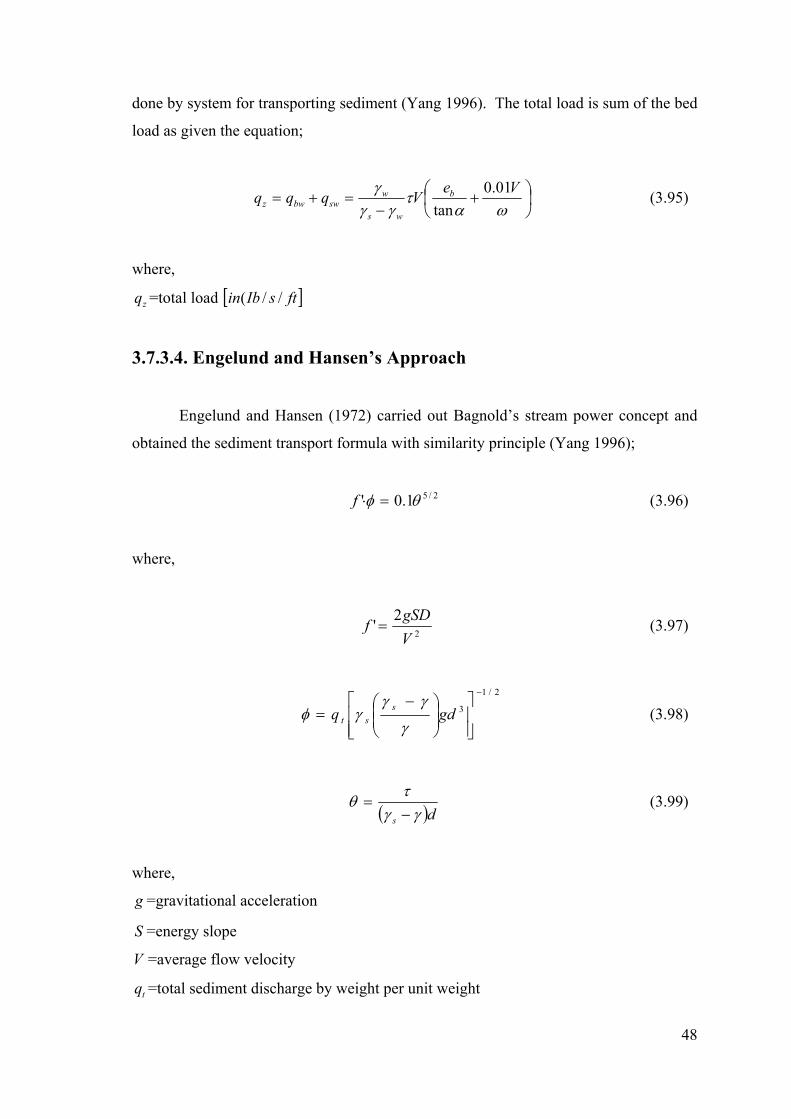
48

done by system for transporting sediment (Yang 1996). The total load is sum of the bed

load as given the equation;

⎟⎠⎞

⎜⎝⎛ +

−=+=

ωατ

γγγ VeVqqq b

ws

wswbwz

01.0tan

(3.95)

where,

zq =total load [ ]ftsIbin //(

3.7.3.4. Engelund and Hansen’s Approach

Engelund and Hansen (1972) carried out Bagnold’s stream power concept and

obtained the sediment transport formula with similarity principle (Yang 1996);

2/51.0' θφ =⋅f (3.96)

where,

2

2'

VgSD

f = (3.97)

2/1

3

−

⎥⎥⎦

⎤

⎢⎢⎣

⎡⎟⎟⎠

⎞⎜⎜⎝

⎛ −= gdq s

st γ

γγγφ (3.98)

( )ds γγτ

θ−

= (3.99)

where,

g =gravitational acceleration

S =energy slope

V =average flow velocity

tq =total sediment discharge by weight per unit weight

49

d =median particle diameter

τ =shear stress along the bed

Engelund and Hansen’s formula is applicable only to dune beds and median

particle diameter is greater than 0.15 mm.

3.7.3.5. Ackers and White’s Approach

Ackers and White (1973) transport capacity formula based on Bagnold’s stream

power concept and applied dimensional analysis for uniform sediment. The

dimensionless sediment transport function is

n

sgr V

U

d

XDG ⎟⎠⎞

⎜⎝⎛= *

γγ (3.100)

where,

X =rate of sediment transport in terms of mass flow per unit mass flow rate (unitless)

D =water depth

*U =shear velocity

d =sediment particle size

V =average flow velocity

Ackers and White (1973) expressed the mobility number for sediment is

( )

n

sngr

dD

VgdUF

−−

⎥⎥⎦

⎤

⎢⎢⎣

⎡

⎥⎥⎦

⎤

⎢⎢⎣

⎡⎟⎟⎠

⎞⎜⎜⎝

⎛−=

12/1

*/log32

1αγ

γ (3.101)

where,

n =transition exponent, depending on sediment size

α =coefficient in rough turbulent equation (=10)

The sediment size by a dimensionless grain diameter is

50

( ) 3/1

2

1/⎥⎦

⎤⎢⎣

⎡ −=

v

gdd s

gr

γγ (3.102)

where,

v =kinematic viscosity

The generalized dimensionless sediment transport function is

m

grgr A

FCG ⎟

⎟⎠

⎞⎜⎜⎝

⎛−= 1 (3.103)

The values, n , A , m and C can be obtained from laboratory data.

If 60>grd (3.104)

025.05.117.00.0

====

CmAn

If 601 ≤< grd (3.105)

( )14.023.0

log56.000.12/1 +=

−=−gr

gr

dA

dn

34.166.9+=

grdm

( ) ( ) 53.3loglog86.2log 2 −−= grgr ddC

Ackers and White’s approach applicable to mmd 04.0> and 8.0<rF .

where,

rF =Froude number

51

CHAPTER 4

ONE DIMENSIONAL HYDRODYNAMIC MODEL

The hydrodynamic model is described by equations of motion in open channel

flows. The flow model is developed to solve governing equations based on conservation

of mass and momentum. The flow depth and velocity of flow are sufficient to define the

flow conditions at a channel cross section, so two governing equations can be solved for

a typical flow situation.

In this Chapter, the continuity and momentum equations are derived that are

usually referred to as the Saint Venant equations.

4.1. de Saint Venant Equations

The one dimensional modeling of unsteady flow in open channels is most often

performed by supplementing de Saint Venant equations that describe the propagation of

a wave. In unsteady modeling, two flow variables, such as the flow depth and velocity

or the flow depth and the rate of flow are calculated to define the flow conditions at a

channel cross section. Therefore, two governing equations must be used to analyze a

typical flow situation. The required equations are the continuity equation and the

momentum equation derived with many assumptions (Roberson, et al. 1997, Chaudry

1993):

● The streamlines do not have sharp curves, so that the pressure distribution is

hydrostatic.

●As the channel bottom slope is small, the measured lateral and vertical velocity

are approximately same, so the lateral velocity and acceleration component can

be neglected.

●No lateral, secondary circulation occurs. The flow velocity distribution is

uniform over any channel cross section.

●The channel is prismatic with the same cross section and slope thorough out

the distance.

52

●The head losses in unsteady flow can be simulated by using the steady – state

resistance laws, so Chezy and Maning equations can be used also in unsteady

flow model. Water has uniform density and flow is generally subcritical

(Chaudhry 1993).

4.1.1. Continuity Equation in Unsteady Flows

According to the law of conservation of mass, both the difference of the rate of

mass inflow through area 1dA at section 1 and the rate of mass outflow through area

2dA at section 2 and the lateral inflow or outflow though xΔ in the same dt time space,

must be equal to changing of volume.

Figure 4.1. Definition sketch for continuity equation

( )( ) 02

1

1211122 =−−−+=∂∂

∫ dxxxqVAVAAdtd

tM x

x

ρρρρ (4.1)

where,

M =mass

A =flow area

21 1q

Flow Control Volume

xΔ x ( )111 ,, QVx ( )222 ,, QVx

dxxVV∂∂

+ V

53

V =flow velocity

ρ =mass density of water

1q =volumetric rate of lateral inflow or outflow per unit length of the channel between

sections 1 and 2. (inflow 1q is positive, outflow 1q is negative)

If water is assumed incompressible, mass density can be taken constant.

Therefore Equation (4.1) becomes,

( )( ) 02

1

1211122 =−−−+∫ dxxxqVAVAAdtd x

x

(4.2)

By rearranging Equation (3.2) with average flow area and average flow velocity

in channel cross section and applying the Leibnitz’s rule *, the equation becomes,

xdtqdtxxVVx

xAAAVdtdt

thxB Δ−⎥⎦

⎤⎢⎣⎡ Δ

∂∂

+⎥⎦⎤

⎢⎣⎡ Δ

∂∂

++−∂∂

Δ 1 (4.3)

where,

h =flow depth

The ⎟⎠⎞

⎜⎝⎛

∂∂

∂∂

xV

xA can be neglected because it is small and with other simplifiers it

becomes,

01 =−∂∂

+∂∂

+∂∂ q

xAV

xVA

thB (4.4)

or

Bq

xhV

xV

BA

th 1=

∂∂

+∂∂

+∂∂ (4.5)

or

54

Bq

xhV

xVh

th 1=

∂∂

+∂∂

+∂∂ (4.6)

For a wide rectangular section the conservation of mass equation for water on a

unit with can be written as:

Bq

xhu

th w1=

∂∂

+∂∂ (4.7)

where,

h =the flow depth (L)

u =the flow velocity (L/T)

wq1 =the lateral flow flux (L2/T)

x =independent variable representing the coordinate in the longitudinal direction (flow

direction) (L)

t =independent variable of time (T)

*Leibnitz’s rule

( )( )

( )

( )

( )

( ) ( )( ) ( )( )dtdfttfF

dtdfttfFdxtxF

tdxtxF

dtd tf

tf

tf

tf

11

22 ,,,,

2

1

2

1

−+∂∂

= ∫∫

4.1.2. Momentum Equation in Unsteady Flows

The second required equation is derived by considering how the forces on the

control volume affect the movement of water through the control volume. The

momentum equation states that the rate of change of momentum is equal to the resultant

force acting on the control volume∑ =dtmvdF )( . In Figure 4.2 there is an element

which has mass m and length xΔ . The rate of changing of total momentum for that

element for the uncompressible flows is,

( )( )∑ ∫ Δ−−−+= xxxqVVAVVAVAdxVdtdF

x

xx

2

1

121111222 ρρρρ (4.8)

55

where,

xV =the component of the velocity of lateral inflow in the x - direction

1q = is positive in lateral inflow and negative in lateral outflow.

The Leibnitz’s rule must be applied to Equation (4.8) and VAQ = ,

( )∑ ∫ ⎟⎠⎞

⎜⎝⎛ −−−+

∂∂

= dxxxqVVQVQdxtQF

x

xx

2

1

1211122 ρρρρ (4.9)

The mean value theorem can save the Equation (4.9) to differential form, so

dividing the terms by ( )12 xx −ρ ,

( )( )

112

qVx

QVtQ

xxF

x−∂

∂+

∂∂

=−

∑ρ

(4.10)

Figure 4.2. Definition sketch for momentum equation

For the typical hydraulic engineering applications the shear stress on the flow

surface due to the wind and the effects of the Coriolis acceleration can be neglected.

The forces acting on the control volume are the pressure forces, the gravity force in the

x - direction and the frictional force which are explained below.

On the upstream end, the pressure force is;

111 hgAF ρ= (4.11)

56

On the downstream end, the pressure force;

222 hgAF ρ= (4.12)

where,

1h and 2h =depth of the centroid of flow area 1A and 2A , respectively

The weight of the water in the control volume in the x - direction is;

∫=2

1

03

x

x

dxASgF ρ (4.13)

where,

0S =The channel bottom slope

The frictional force due to water and the channel sides and channel bottom is;

dxASgFx

xf∫=

2

1

4 ρ (4.14)

where,

fS =The friction slope

The resultant force acting on the control volume is;

∑ −+−= 4321 FFFFF (4.15)

By inserting terms in the Equation (4.15) and dividing by ( )12 xx −ρ ,

( )( ) ( )dxSSA

xxg

xxhAhAg

xxF x

xf∫∑ −

−+

−−

=−

2

1

01212

2211

12ρ (4.16)

The mean value theorem can save the Equation (4.16) to differential form,

57

( ) ( ) ( )fx SSgAhAx

gqVx

QVtQ

−+∂∂

−=−∂

∂+

∂∂

01 (4.17)

By rearranging gives,

( ) ( ) 10 qVSSgAhgAQVxt

Qxf +−=+

∂∂

+∂∂ (4.18)

The Equation 4.18 is the momentum equation of water flow. If the right – hand

side of this equation is zero, it means that mass is conserved along any closed contour in

the tx − plane unless it is zero, this term acts like a source or a sink depending on 1q

(Cunge, et al. 1980).

( ) ( ) ( ) hAhBhhAhA −⎥⎦⎤

⎢⎣⎡ Δ−Δ+=Δ 2

21 (4.19)

So the higher – order terms can be neglected. Assuming 0→Δh , we can obtain

( )( ) AhAh =∂∂ and that can be rearranged as:

( ) ( )xhgA

xhhA

hghgA

x ∂∂

=∂∂

∂∂

=∂∂ (4.20)

The Equation 4.18 becomes,

( ) ( )fx SSgAqVxhgA

xQV

tQ

−+=∂∂

+∂

∂+

∂∂

01 (4.21)

The acceleration can be an increase in velocity at one point over time (local

acceleration) or an increase in velocity over space (acceleration may occur as water

moves along the control volume). These concepts lead to the de Saint Venant Equations,

the momentum equation, which when written in its conservation form is (Chaudhry

1993).

58

( )fSSghg

Vx

gtV

−=⎟⎟⎠

⎞⎜⎜⎝

⎛+

∂∂

+∂∂

0

2

2 (4.22)

Rearranging of the terms gives;

( ) 00 =−−∂∂

+∂∂

+∂∂

fSSgxhg

xVV

tV (4.23)

For steady uniform flow, the friction slope is equal to channel bottom slope. The

equation for steady, gradually varied flow is obtained by including the variation of the

flow depth and velocity head by including the derivative with respect to distance x . The

unsteadiness or the local acceleration term is needed to make the equation valid for

unsteady nonuniform flow model.

0SS f = xh∂∂

− ⎟⎟⎠

⎞⎜⎜⎝

⎛∂∂

−g

Vx 2

2

tV

g ∂∂

−1 (4.24)

de Saint Venant equations are nonlinear equations for which numerical methods

are required to solve them, so they were not practically applied in their full

Steady, nonuniform

Quasi-Steady Dynamic Wave Aprox.

Steady, uniform

Kinematic Wave Aprox.

Steady, nonuniform

Diffusion Wave Aprox.

Unsteady, nonuniform

Full Dynamic Wave Equation

Local Acceleration Term

Convective Acceleration Term

Pressure Force Term

Gravity Force Term

Friction Force Term

59

hydrodynamic form until the 1950s, although they were derived in the early nineteenth

century. A number of simplifications were performed by different researchers, being

more appropriate in particular situations. Consideration of the implications of the

different simplifications can also lead to a better understanding of the full equations so

de Saint Venant equations were described by the propagation of a wave. In wave

approximations, the continuity equation is solved simultaneously with approximate

form of the momentum equation. Their differences are all in momentum equation

assumptions. The three types of simplifications for wave models studied in this research

are summarized below.

4.2. Kinematic Wave Approximation

The kinematic wave approximation represents the change of flow with distance

and time by neglecting the local and convective acceleration terms of the momentum

equation. The assumption is that the water surface is parallel to the channel bed

(uniform flow assumption) in the kinematic wave approximation. It means there is no

way to represent backwater effects. These assumptions reduce the momentum equation

to the following.

fSS =0 (4.25)

The remaining terms represent the resistance equation for steady, uniform flow

as described by Manning’s or Chezy’s equation but can be taken into consideration the

effects of unsteadiness by an increase or decrease in the flow depth.

The resistance equation can be written as:

)(AfQ = (4.26)

By applying the chain rule we can write,

tQ

QA

tA

∂∂

∂∂

=∂∂ (4.27)

60

0xxQA

tQ

tA

=∂∂

∂∂

=∂∂ (4.28)

Substituting this equation into Equation 4.6, assuming 01 =q ,

0=∂∂

+∂∂

xqa

tQ (4.29)

where,

dAdQa = Represents the velocity of flood wave (L2/T)

This equation represents the kinematic wave which’s combined with continuity

equation. While Q is dependent variable, x and t are independent variables in this first

– order partial differential equation. If a is constant, the equation becomes linear. The

general solution of this linear equation by D’Alembert is,

)( atxfQ −= (4.30)

While 0=t , it represents initial conditions. The function creates a curve that

describes the variation of discharge Q with distance x . Assuming that t changes such as,

1t , 2t and 3t at velocity a in the downstream direction, the discharge occurs 1Q , 2Q and

3Q drawing a curve. It can be said that this curve always appears as )(xf , so it shows a

flood hydrograph in kinematic wave as it travels in the positive x - direction at velocity

a , the shape of the hydrograph does not change and its peak does not attenuate

(assuming a is constant). The kinematic wave equation describes the propagation of a

flood wave along a river reach but doesn't account for any backwater effects. This

implies that water may only flow downstream. The solution may be analytical or

numerical (Chaudhry 1993).

4.3. Diffusion Wave Approximation

The diffusion wave approximation is a simplified form of the dynamic wave

approximation. In addition, it is a significant improvement over the kinematic wave

61

model. In the diffusion wave approach, the th ∂∂ term from de Saint Venant equation

allows the water – surface slope to differ from the bed slope. This pressure differential

term allows the diffusion model to describe the attenuation of the floodwave. It also

allows the specification of a boundary condition at the downstream extremity of the

routing reach to account for backwater effects. The simplified form of the momentum

equation includes the convective acceleration term representing the spatial change in the

flow depth as well as the source terms, but neglects the temporal derivative term as well

as the convective acceleration terms due to spatial change in the flow velocity

(Chaudhry 1993). The simplified form of the momentum equation is,

)( 0 fSSxh

−=∂∂ (4.31)

Combining the simplified momentum equation with the continuity equation

gives the single equation called the diffusion wave equation.

xQa

tQ

xQD

∂∂

+∂∂

=∂∂

2

2

(4.32)

where,

02BSQD =

dAdQa =

The first term of the right side in this equation is the same as the equation for

kinematic model. The first term of the left side in Equation 4.32 represents the diffusion

of a flood wave as it travels in the channel. The coefficients D and a determined from

the observed hydrographs. By using them the attenuation of a flood wave due to storage

and friction can be included in the analysis (Chaudhry 1993).

4.4. Dynamic Wave Approximation

The dynamic wave equations are most accurate and comprehensive solution for

one dimensional unsteady flow problems in open channels under the specific

assumptions. The dynamic wave equations can be applied to wide range of one

dimensional flow problems such as dam break flood wave routing, evaluating flow

62

conditions due to tidal fluctuations, and routing flows through irrigation and canal

systems. The full equations can be solved by several numerical methods for incremental

times t and incremental distances x along the water way. The specific terms in the

momentum equation are small in comparison to the bed slope. In dynamic wave

approximation, the continuity equation is solved simultaneously with approximate form

of the momentum equation. If we reorganize the momentum equation Equation 4.24 the

full dynamic wave approximation can be defined by,

)( 0 fSSgxhg

xuu

tu

−=∂∂

+∂∂

+∂∂ (4.33)

where,

u =the flow velocity (L/T)

h =the flow depth (L)

=fS friction slope

=0S bed slope

g =acceleration due to gravity )/( 2TL

t =independent variable of time (T)

x =independent variable representing the coordinate in the longitudinal direction (flow

direction) (L)

63

CHAPTER 5

ONE DIMENSIONAL SEDIMENT TRANSPORT MODEL

The bed of the channel may aggrade or degrade in natural streams if the balance

of the water discharge or sediment is destroyed by natural or manmade factors. Eroding

loose surface from the basin by water deteriorates the ecology and changes the river

morphology. The water level rises and brings ecological problems when sediments are

deposited in river basins. It is essential to predict effects of sediment transport for river

management. Current research on river sediment transport prediction is mainly based on

numerical modeling of sediment transport. One dimensional unsteady sediment transport

models studied in two categories in this research: equilibrium and nonequilibrium.

5.1. One Dimensional Numerical Model for Sediment Transport under

Unsteady and Equilibrium Conditions

Bed material transportation is mathematically divided into two independent

processes: erosion and deposition. When the erosion and the deposition rates are equal

then there is equilibrium. It means that there is no interchange of sediment particles

between suspended and bed load sediment transport (Tayfur and Singh 2007). The

equilibrium condition exists when the same number of a given type and size of particles

are deposited on the bed as are entrained from it. In the literature, most of the studies are

based on equilibrium approach although natural rivers are mostly in nonequilibrium

state. When flow and sediment discharges, channel geometry and sediment properties

do not change substantially a long period of time, assuming the equilibrium sediment

transport conditions is appropriate.

5.1.1. Kinematic Wave Model of Bed Profiles in Alluvial Channels

under Equilibrium Conditions

The kinematic wave model neglects the local acceleration, convective

acceleration and pressure terms in the momentum equation for dynamic wave model.

64

Tayfur and Singh (2006) represented transport movement in a wide rectangular alluvial

channels as a system involving two layers: water flow layer and movable bed layer, as

shown in Figure 5.1. The water flow layer may contain suspended sediment. The

movable bed layer consists of both water and sediment particles, so the movable bed

layer includes porosity. The basic one dimensional partial differential equations for

unsteady and equilibrium nonuniform transport can be expressed as (Tayfur and Singh

2006):

Figure 5.1 Definition sketch of two layer system

(Source: Tayfur and Singh 2006)

● Continuity equation for water:

wqtzp

xchu

tch

1)1()1(

=∂∂

+∂−∂

+∂−∂ (5.1)

where,

u = flow velocity (L/T)

h = flow depth (L)

z = mobile bed layer elevation (L)

c = volumetric sediment concentration in the water flow phase (in suspension) ( 33 / LL )

wq1 =volumetric rate of lateral inflow or outflow of water (L/T)

p =porosity of the bed layer ( 33 / LL )

z

h water flow layer

movable bed layer

fixed bed layer

65

t =independent variable of time (T)

x =independent variable representing the coordinate in the longitudinal direction (flow

direction) (L)

● Continuity equation for sediment:

( ) sbs qx

qtzp

xhuc

thc

11 =∂∂

+∂∂

−+∂∂

+∂∂ (5.2)

where,

bsq =the sediment flux in the movable bed layer )/( 2 TL

sq1 =volumetric rate of lateral inflow or outflow of sediment (L/T)

For simplicity, if there is no lateral inflow of water and sediment, the terms on

the right hand sides of Equation 5.1 and Equation 5.2 vanish (Tayfur and Singh 2006).

Equations 5.1 and 5.2 contain five unknowns: zcuh ,,, and bsq . It means that

there must be three additional equations. One equation is obtained from momentum

equation for kinematic wave which is given as follows:

● Momentum equation for water:

of SS = (5.3)

Friction slope is taken as equal to bed slope employing Chezy’s equation for the

friction slope, yields;

1−= βαhu (5.4)

where, 5.0

fzSC=α

5.1=β

The second equation is obtained from Velikanov (1954), relating suspended

sediment concentration to flow variables as;

hgvuc

f

3κ= (5.5)

66

where,

g =gravitational acceleration (L/T2)

fv = average fall velocity of sediments (L/T)

κ = coefficient of sediment transport capacity

By rearranging the equation with fgv

κδ = , the equation becomes,

13 −= huc δ (5.6)

The third equation is obtained from Langbein and Leopold (1968) who proposed

a sediment flux concentration relation as:

⎥⎥⎦

⎤

⎢⎢⎣

⎡−=

max

1b

bbsst C

CCvq (5.7)

where,

stq = sediment transport rate (M/L/T)

sv = velocity of sediment particles as concentration approaches zero (L/T)

bC = areal sediment concentration (M/L2)

maxbC = maximum areal sediment concentration (M/L2)

The sediment transport rate stq is in (M/L/T) (Equation 5.7) and the sediment flux

bsq is in (L2/T) (Equation 5.2), so stq is related to bsq as:

bssst qq ρ= (5.8)

where,

sρ = mass density of sediment (M/L3)

Areal concentration can be related to bed level as (Tayfur and Singh 2006):

( ) sb zpC ρ−= 1 (5.9)

67

By substituting Equations 5.8 and 5.9 into the Equation 5.7;

( ) ⎥⎦

⎤⎢⎣

⎡−−=

max

11z

zzvpq sbs (5.10)

where,

maxz = maximum bed elevation (L)

By using the chain rule, derivative of bsq can be obtained as:

( )xz

zzvp

xq

sbs

∂∂

⎥⎦

⎤⎢⎣

⎡−−=

∂∂

max

211 (5.11)

Hence the unknowns zcuh ,,, and bsq can be obtained by the system of

Equations 5.1, 5.2, 5.4, 5.5 and 5.11. After algebraic manipulation, the equations can be

written in compact form as:

[ ] [ ] 05.15.15.11 45.05.03 =∂∂

+∂∂

−+∂∂

−tzp

xhhh

thh δααδα (5.12)

[ ] [ ] ( ) ( ) 0211125.1max

45.03 =∂∂

⎥⎦

⎤⎢⎣

⎡−−+

∂∂

−+∂∂

+∂∂

xz

zzvp

tzp

xhh

thh sδαδα (5.13)

(note that 5.1=β )

5.1.1.1. Numerical Solution of Kinematic Wave Equations

In this model, a finite difference scheme developed by Lax (1954) is used. This

scheme can capture shocks, since all the governing equations are solved simultaneously.

There is no need for iterations when gradients are large. The Lax scheme is an explicit

scheme and does not require large matrices, so it is easy for solving general empirical

equations for roughness and sediment discharge. With reference to the finite difference

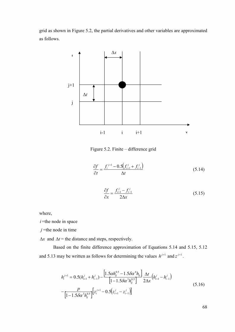
68

grid as shown in Figure 5.2, the partial derivatives and other variables are approximated

as follows.

Figure 5.2. Finite – difference grid

( )t

ffftf j

ij

ij

i

Δ+−

=∂∂ −+

+11

1 5.0 (5.14)

xff

xf j

ij

i

Δ−

=∂∂ −+

211 (5.15)

where,

i =the node in space

j =the node in time

xΔ and tΔ = the distance and steps, respectively.

Based on the finite difference approximation of Equations 5.14 and 5.15, 5.12

and 5.13 may be written as follows for determining the values 1+jh and 1+jz .

[ ][ ] ( )

[ ] ( )[ ]ji

ji

ji

ij

ji

ji

ij

ijijji

ji

ji

zzzh

p

hhxt

hhh

hhh

111

5.03

115.03

45.0

111

5.05.11

25.115.15.1

)(5.0

−++

−+−++

−−−

−

−ΔΔ

−−

−+=

δα

δαδαα

(5.16)

tΔ

i+1 i-1 i x

xΔ t

j+1

j

69

[ ] ( )[ ]( ) ( )[ ] ( )j

ij

iij

sj

ij

ij

iij

ji

ji

ijji

ji

ji

zzxt

zz

vhhhph

hhxt

ph

zzz

11max

111

5.03

11

4

111

22

15.01

5.12

2)(5.0

−+−++

−+−++

−ΔΔ

⎥⎦

⎤⎢⎣

⎡−−−−

−−

−ΔΔ

−+=

δα

δα

(5.17)

The hydrodynamic part of the model is:

[ ][ ] ( )j

ij

iij

ijijji

ji

ji hh

xt

hhh

hhh 115.03

45.0

111

25.115.15.1

)(5.0 −+−++ −

ΔΔ

−−

−+=δα

δαα (5.16a)

111 )( −++ = βα j

ij

i hu (5.16b)

By using the presented algorithm, the unknown values of h and z at the new

time level 1+j (future time) are determined from every interior node ( i = 2,…….,N-1).

The values of the dependent variables h and z at the boundary nodes 1 and N+1 are

determined by using boundary conditions. Also, at the time level j =1, initial conditions

are already known.

Initial conditions can be specified as:

( ) ohxh =0, (5.18)

( ) ozxz =0, (5.19)

where,

oh and oz = the initial flow depth (L) and the bed level (L), respectively.

The upstream boundary conditions can be specified as inflow hydrograph and

inflow sedimentograph.

( ) )(,0 thth = (5.20)

70

( ) )(,0 tztz = (5.21)

The downstream boundary conditions can be specified as:

( ) 0),(=

∂∂

xtNh ( 1

111

+−

++ = j

Nj

N hh ) 0.0>t (5.22)

( ) 0),(=

∂∂

xtNz ( 1

111

+−

++ = j

NjN zz ) 0.0>t (5.23)

●Stability

The numerical scheme has to satisfy the stability conditions. For this reason, the

Courant – Friedrichs – Lewy (CFL) condition was used. Since the water waves travel at

a much higher velocity than the bed transients this condition is given by:

( )1≤

ΔΔ+

=x

tghuCn (5.24)

where,

nC = Courant number (it was taken 2.0=nC in this research)

Equations 5.16 and 5.17 are solved simultaneously for each time step.

5.1.1.2. Model Testing for Hypothetical Cases

The hypothetical cases were analyzed assuming inflow hydrograph and

concentration at the upstream of the channel, shown in Figures 5.3a and 5.3b.

The channel was assumed to have a 1000 m length and 20 m width with 0.0025

bed slope. Chezy roughness coefficient is 50=zC m0.5/s. The sediment was assumed to

have 2650=sρ kg/m3, 32.0=sd mm, 48.0=p and sediment transport capacity

coefficient 000075.0=κ (Ching and Cheng 1964). Langbein and Leopold (1968)

suggest 245max =C kg/m2 (note that sb zpC ρ)1( −= ). In Figure 4.3b, 14=bC kg/m2

corresponds the bed level 01.0=z m and 140=bC kg/m2 corresponds the bed level

10.0=z m.

71

0

50

100

150

200

250

0 30 60 90 120 150 180 210 240 Time (min)

Q (m3/s)

020406080

100120140160

0 30 60 90 120 150 180 210 240 Time (min)

C (kg/m2)

Figure 5.3. (a) Inflow hydrograph (b) Inflow concentration

5.1.1.2.1. Hypothetical Case I: Effect of Inflow Concentration

Figure 5.4a shows that when the inflow concentration increases at the upstream

end of the channel, bed level gradually increases. In the Figure 5.4b when the

equilibrium feeding of the sediment occurs at the upstream, the bed level continues to

increase along the channel length. During the recession limp of the inflow concentration

the bed level starts to decrease toward the 10% length of the channel while it increases,

toward the 90% length of the channel (Figure 5.4c). Figure 5.4d shows that the bed

level decreases to the original level at the upstream section but as time progresses it

increases toward the downstream section.

a

b

72

0

0,02

0,04

0,06

0,08

0,1

0 200 400 600 800 1000

Distance (m)

Bed

Lev

el z

(m) 20 min

40 min60 min

0

0,02

0,04

0,06

0,08

0,1

0,12

0 200 400 600 800 1000

Distance (m)

Bed

Lev

el z

(m) 80 min

100 min

0

0,02

0,04

0,06

0,08

0,1

0 200 400 600 800 1000

Distance (m)

Bed

Lev

el z

(m)

120 min140 min160 min

0

0,02

0,04

0,06

0,08

0,1

0 200 400 600 800 1000

Distance (m)

Bed

Lev

el z

(m)

180 min200 min220 min240 min

Figure 5.4. Transient bed profile at (a) rising period (b) equilibrium period (c) recession period

(d) post recession period of inflow hydrograph and concentration

c

b

a

d

73

5.1.1.2.2. Hypothetical Case II: Effect of Particle Velocity and Effect

of Particle Fall Velocity

The objective of this case was to compare the sediment particle velocity and

particle fall velocity formulations employed in the developed model. The fall velocity

must be obtained for calculating the particle velocity. For that reason, first of all we

wanted to see four particle velocity formulation’s (in literature) performances under the

Rouse (1938)’s fall velocity formulation. The fall velocity value is for most natural

sands of the shape factor of 0.7 and 2.0=sd mm is 024.0=fv m/s (Rouse 1938).

Under the same particle fall velocity, the developed model was tested for four different

particle velocity formulations (Bor, et al. 2008).

One of the formulations is Chien and Wan (1999) formulation. For

mmd s 1008.0 << and 1550/10 << sdh , Chien and Wan (1999) presented the

following relation:

2

3)4.1/(u

uuv c

s −= (5.25)

where,

cu = critical flow velocity at the incipient sediment motion (L/T).

cu can be expressed as a function of the particle fall velocity fv and the shear

velocity Reynolds number *R as (Yang 1996):

⎪⎩

⎪⎨

⎧+

−=

f

ff

c

v

vR

vu

05.2

66.006.0)log(

5.2*

70702.1

*

*

>

<<

RR (5.26)

The shear velocity Reynolds number *R (Yang 1996):

υsdu

R ** = (5.27)

74

where,

υ = kinematic viscosity of water (L2/T)

*u = shear velocity (L/T) and defined as (Yang 1996):

oghSu =* (5.28)

The second selected formulation is Bridge and Dominic (1984) formulation that

is derived though a theoretical consideration of the dynamics of bed load motion.

)( ** cs uuv −= δ (5.29)

where,

cu* = critical shear velocity (L/T). Bridge and Dominic (1984) expressed the average

value of δ between 8 and 12. In this study the employed is 10=δ . The critical shear

velocity defined as (Bridge and Dominic 1984):

δφ 2

*

)(tanfc

vu = (5.30)

where,

=φtan the dynamic friction coefficient (average value between 0.48 and 0.58 (Bridge

and Dominic 1984). In this study =φtan 0.53 was employed.

The third selected was a constant particle velocity is smvs /010.0= .

The fourth particle velocity equation is Kalinske’s equation. Kalinske (1947)

assumed that

( )cs uubv −= (5.31)

where,

uvs , = instantaneous velocities of sediment and fluid

cu = critical flow velocity at incipient motion

b = a constant close to unity

75

Secondly we wanted to see these four particle velocity formulation’s

performances under the Dietrich (1982) fall velocity formulation (Bor, et al. 2008).

)(

3*2110 RRRW += (5.32)

where,

*W = the dimensionless fall velocity of the particle

The fall velocity of particle is (Dietrich 1982):

31

* )(⎟⎟⎠

⎞⎜⎜⎝

⎛ −=

ρυρρ gW

v sf (5.33)

4*

3*

2**1

)(log00056.0

)(log00575.0)(log0982.0)(log929.1767.3

D

DDDR

+

−−+−= (5.34)

)6.4(log)1)(5.0(3.0

]6.4tanh[log)1(85.0

)1(1log

*2

*3.2

2

−−−+

−−−⎥⎦⎤

⎢⎣⎡ −−=

DCSFCSF

DCSFCSFR (5.35)

⎥⎦⎤

⎢⎣⎡ −+

⎥⎦

⎤⎢⎣

⎡⎟⎠⎞

⎜⎝⎛ −−=

5.2)5.3(1

*3 ]6.4tanh[log83.2

65.0

P

DCSFR (5.36)

where,

*D = the dimensionless particle size

CSF = the Corey shape factor. The mean value of CSF for most naturally occurring

sediment is between 0.5 and 0.8 (Dietrich 1982). This study employed a value of

65.0=CSF .

P = the Powers value of roughness (the average value of 6~5.3=P (Dietrich 1982)).

This study employed the value of 75.4=P .

The dimensionless particle size is expressed as (Dietrich 1982):

76

2

3

*)(

ρυρρ ss gd

D−

= (5.37)

The third selected particle fall velocity formulation is Yang (1996) formulation.

We wanted to see these four particle velocity formulation’s performances under the

Yang (1996)’s fall velocity formulation (Bor. et al, 2008).

⎪⎪⎪⎪

⎩

⎪⎪⎪⎪

⎨

⎧

⎥⎦

⎤⎢⎣

⎡ −

−

=

s

w

wss

s

w

ws

f

d

gdF

gd

v

32.3

)(

)(181

5.0

2

γγγ

υγγγ

mmd

mmdmm

mmd

s

s

s

0.2

0.21.0

1.0

>

≤<

≤

(5.38)

where,

5.0

3

25.0

3

2

)(36

)(36

32

⎪⎩

⎪⎨⎧

⎥⎦

⎤⎢⎣

⎡−

−⎥⎦

⎤⎢⎣

⎡−

+=wss

w

wss

w

gdgdF

γγγυ

γγγυ

(5.39)

In Figures 5.5a, 5.5b and 5.5c it is seen that while Kalinske (1947) and Bridge

and Dominic (1984) formula give a faster wavefront, constant smvs /01.0= and Chien

and Wan (1999) formula give slower wavefront in rising and equilibrium period. At

recession period, as the sediment feeding decreases the bed elevation starts to decrease

toward the upstream section (in 20% of the channel length) under constant

smvs /01.0= . It is seen that Kalinske (1947) and Bridge and Dominic (1984) formula

give similar performance and sediment moves faster towards downstream end. This is

reasonable, since the transient bed profile moves downstream and thus concentration

also increases downstream (Figure 5.5c). In the postrecession period, the bed level

increases to original bed level at the upstream section. It is seen that bed profile reached

original bed early with Kalinske (1947) and Bridge and Dominic (1984) formula

(Figure 5.5d) (Bor, et al. 2008).

The same simulations were obtained under the other three fall velocity

formulations.

77

t=80min the fall velocity is "Rouse"

0

0,02

0,04

0,06

0,08

0,1

0,12

0 100 200 300 400 500 600 700 800 900 1000Distance (m)

Bed

Lev

el z

(m)

Vs=0.010 m/sVs=Chien&WanVs=Bridge&DominicVs=Kalinske

t=40min the fall velocity is "Rouse"

0

0,01

0,02

0,03

0,04

0,05

0,06

0 100 200 300 400 500 600 700 800 900 1000Distance (m)

Bed

Lev

el z

(m)

Vs=0.010 m/sVs=Chien&WanVs=Bridge&DominicVs=Kalinske

t=160min the fall velocity is "Rouse"

0

0,02

0,04

0,06

0,08

0,1

0 100 200 300 400 500 600 700 800 900 1000Distance (m)

Bed

Lev

el z

(m)

Vs=0.010 m/sVs=Chien&WanVs=Bridge&DominicVs=Kalinske

t=240min the fall velocity is "Rouse"

0

0,02

0,04

0,06

0,08

0 100 200 300 400 500 600 700 800 900 1000Distance (m)

Bed

Lev

el z

(m)

Vs=0.010 m/sVs=Chien&WanVs=Bridge&DominicVs=Kalinske

Figure 5.5. Transient bed profile under different particle velocities at (a) rising period (b)

equilibrium period (c) recession period (d) postrecession period of inflow

hydrograph and concentration. (Source: under Rouse 1938, Dietrich 1982, Yang

1996 formula).

a

b

c

d

78

t=40 min "Chien & Wan" the particle velocity approach

0

0,01

0,02

0,03

0,04

0,05

0,06

0 200 400 600 800 1000Distance (m)

Bed

Lev

el z

(m)

Dietrich Yang Rouse

t=80 min "Chien & Wan" the particle velocity approach

0

0,02

0,04

0,06

0,08

0,1

0,12

0 200 400 600 800 1000Distance (m)

Bed

Lev

el z

(m)

Dietrich Yang Rouse

t=160 min "Chien & Wan" the particle velocity approach

0

0,02

0,04

0,06

0,08

0,1

0 200 400 600 800 1000Distance (m)

Bed

Lev

el z

(m)

Dietrich Yang Rouse

t=240 min "Chien & Wan" the particle velocity approach

0

0,02

0,04

0,06

0,08

0 200 400 600 800 1000Distance (m)

Bed

Lev

el z

(m)

Dietrich Yang Rouse

Figure 5.6. Transient bed profiles under different fall velocities at (a) rising period (b)

equilibrium period (c) recession period (d) postrecession period of inflow

hydrograph and concentration. (Source: under Chien and Wan 1999, Bridge and

Dominic 1984, Kalinske 1947 formulation.

a

b

c

d

79

In Figure 5.6a, 5.6b and 5.6c, the effect of the fall velocity on the sediment

transport under the different particle velocity formulations is given. Dietrich (1982),

Yang (1996) fall velocity formulations and constant smv f /024.0= value (Rouse

1938) give nearly same result under the Bridge and Dominic (1984), Kalinske (1947),

and Chien and Wan (1999) particle velocity formulation. For better assessment, the

model must be test with experimented results (Bor, et al. 2008).

The same simulation profiles were obtained under the other three particle

velocity formulations.

5.1.1.2.3. Hypothetical Case III: Effect of Maximum Concentration

In this case, different maximum concentration values were tested using

developed kinematic wave model. For that reason, 2max /840 mkgC = (corresponds to

maximum bed level of mz 60.0max = ), 2max /630 mkgC = (corresponds to maximum bed

level of mz 45.0max = ), 2max /420 mkgC = (corresponds to maximum bed level of

mz 30.0max = ) and 2max /245 mkgC = (corresponds to maximum bed level of

mz 17.0max = ) were selected respectively. It is seen in Figure 5.7 that higher maxz value

gives higher bed level in the transient bed form profile. The sediment particles move

faster downstream under high bed level. The bed levels increased gradually and

wavefronts moved slowly at the rising and equilibrium periods of the simulation (Figure

5.7a and 5.7b). At 160 min while the bed wavefront just reached about 400 m

under mz 15.0max = , it moved the downstream end under mz 60.0max = (Figure 5.7c).

While the front under mz 30.0max = closely followed the front under mz 17.0max = , front

under mz 45.0max = closely followed the front under mz 60.0max = (Figure 5.7a-5.7c).

80

0

0,01

0,02

0,03

0,04

0,05

0,06

0 200 400 600 800 1000Distance (m)

Bed

Lev

el z

(m)

t=40 min zmax=0.17 m t=40 min zmax=0.30 mt=40 min zmax=0.45 m t=40 min zmax=0.60 m

0

0,02

0,04

0,06

0,08

0,1

0,12

0 200 400 600 800 1000Distance (m)

Bed

Lev

el z

(m)

t=80 min zmax=0.17 m t=80 min zmax=0.30 mt=80 min zmax=0.45 m t=80 min zmax=0.60 m

0

0,02

0,04

0,06

0,08

0,1

0,12

0 200 400 600 800 1000

Distance (m)

Bed

Lev

el z

(m)

t=160 min zmax=0.17 m t=160 min zmax=0.30 mt=160 min zmax=0.45 m t=160 min zmax=0.60 m

0

0,02

0,04

0,06

0,08

0 200 400 600 800 1000Distance (m)

Bed

Lev

el z

(m)

t=240 min zmax=0.17 m t=240 min zmax=0.30 mt=240 min zmax=0.45 m t=240 min zmax=0.60 m

Figure 5.7. Transient bed profile under different maxz values at (a) rising period (b) equilibrium

period (c) recession period (d) postrecession period of inflow hydrograph and

concentration

d

c

a

b

81

5.1.2. Diffusion Wave Model of Bed Profiles in Alluvial Channels

under Equilibrium Conditions

The diffusion wave model neglects only the local and convective accelerations

in the dynamic wave momentum equation. It is the simplified form of the momentum

equation which includes also pressure force term. Thus, the momentum equation with

these simplifications for a wide rectangular alluvial channel with two layers (Figure 5.1)

becomes:

● Momentum equation for water

)( 0 fSSgxzg

xhg −=

∂∂

+∂∂ (5.40)

The flow velocity in open channels for diffusion waves can be calculated by

using either the Manning or Chezy’s formulations. We express as 1−= βαhu , α here

becomes:

5.0

⎟⎠⎞

⎜⎝⎛

∂∂

−∂∂

−=xz

xhSC ozα (5.41)

The algorithms for 1+jih and 1+j

iz is presented before by Equations 5.16 and 5.17.

The additional algorithm jfiS is determined as:

( ) ( )xzz

xhhSS

ji

ji

ji

ji

ojfi Δ

−−

Δ−

−= −+−+

221111 (5.42)

The hydrodynamic part of the model is:

( )xhhSS

ji

ji

ojfi Δ

−−= −+

211 (5.42a)

Equations 5.16, 5.17 and 5.42 are solved simultaneously for each time step.

82

5.1.2.1. Numerical Solution of Diffusion Wave Equation

Finite difference scheme developed by Lax (1954) is used in this model. The

partial derivatives were explained before in Equations 5.14 and 5.15. Initial and

boundary conditions were specified before Equations 5.18 – 5.23. And for stability the

Courant – Friedrichs – Lewy (CFL) condition was used.

5.1.3. Dynamic Model of Bed Profiles in Alluvial Channels under

Equilibrium Conditions

Conservation of mass equations for bed sediment in the movable bed layer,

considering there is no exchange of sediment due to the detachment and deposition

between two layers, and water for a wide rectangular alluvial channel:

● Continuity equation for water assuming that clear water ( )0=c :

wqxhu

xuh

th

1=∂∂

+∂∂

+∂∂ (5.43)

● Continuity equation for sediment:

sbs qx

qtzp

xhuc

thc

1)1( =∂∂

+∂∂

−∂∂

+∂∂ (5.44)

● Momentum equation for water

The one dimensional partial differential momentum equation of unsteady,

equilibrium flow in alluvial channel with dynamic wave assumption is;

)( 0 fSSgxzg

xhg

xuu

tu

−=∂∂

+∂∂

+∂∂

+∂∂ (5.45)

The friction slope fS in Equation 5.45 can be determined using the Chezy

equation (Equation 3.38).

83

5.1.3.1. Numerical Solution of Dynamic Wave Equations

In dynamic model, a finite difference scheme developed by Lax (1954) is used,

as explained as before. With reference to the finite difference grid as shown in Figure

5.2, additional to the partial derivatives, the variables are jih , j

iu , jiz and j

fiS are

approximated as follows:

( )ji

ji

ji hhh 112

1−+ += (5.46)

( )ji

ji

ji uuu 112

1−+ += (5.47)

( )jif

jif

jif SSS

1121

−++= (5.48)

Under the assumption there is no suspended sediment (clear water flow ( )0=c ),

the first and second term on the right side of the Equation 5.44 will disappear. Based on

the finite difference approximation of (5.14), (5.15), (5.46), (5.47) and (5.48), Equations

5.43 - 5.45 may be written as follows for determining the values 1+jh , 1+jiu and 1+jz :

( ) ( ) ( )ji

ji

ji

ji

ji

ji

ji

ji

ji hhu

xtuuh

xthhh 111111

1 5.05.05.0 −+−+−++ −

ΔΔ

−−ΔΔ

−+= (5.49)

( ) ( ) ( )

( ) ( )jfio

ji

ji

ji

ji

ji

ji

ji

ji

ji

ji

SStgzzgxt

hhgxtuuu

xtuuu

−Δ+−ΔΔ

−

−ΔΔ

−−ΔΔ

−+=

−+

−+−+−++

11

1111111

5.0

5.05.05.0 (5.50)

The hydrodynamic part of the model is:

( ) ( ) ( ) ( )jfio

ji

ji

ji

ji

ji

ji

ji

ji SStghhg

xtuuu

xtuuu −Δ+−

ΔΔ

−−ΔΔ

−+= −+−+−++

1111111 5.05.05.0 (5.50a)

84

( ) ( ) ( )ji

ji

ji

sj

ij

ij

i zzpz

zpv

xtzzz 11

max11

1

1

215.05.0 −+−+

+ −−

⎥⎦

⎤⎢⎣

⎡−

ΔΔ

−+= (5.51)

(note that bsq express as before Equation 5.11)

By using the presented algorithm, the unknown values of h and z at the new

time level 1+j (future time) are determined from every interior node ( i = 2,…….,N-1).

The values of the dependent variables h and z at the boundary nodes 1 and N+1 are

determined by using boundary conditions. Also, at the time level j =1, initial conditions

are already known.

Initial and boundary conditions were specified before Equations 5.18 – 5.23.

And for stability the Courant – Friedrichs – Lewy (CFL) condition was used.

Equations 5.49, 5.50 and 5.51 are solved simultaneously for each time step.

Note that, in the case of Dynamic Wave, we assumed that there is no suspended

sediment.

5.1.3.2. Model Testing: Comparing the Kinematic, Diffusion and

Dynamic Models for Hypothetical Cases

The hypothetical cases were analyzed assuming inflow hydrograph and

concentration at the upstream of the channel as shown in Figures 5.3a and 5.3b. The

channel was assumed to have a 1000 m length and 20 m width with 0.0025 bed slope.

Chezy roughness coefficient 50=zC m0.5/s and Manning roughness coefficient

31

021.0 −= smn . The sediment was assumed to have 2650=sρ kg/m3, 32.0=sd mm,

528.0=p and sediment transport capacity coefficient 000075.0=κ (Ching and Cheng,

1964). Langbein and Leopold (1968) suggest 245max =C kg/m2 (note that

sb zpC ρ)1( −= ).

For three of wave solutions a Courant number was selected 0.2. The numerical

solutions are plotted mx 200= , mx 500= and mx 800= along the channel, respectively

(Figure 5.8 and Figure 5.9). By comparing Figures 5.8a, 5.8b and 5.8c, one can observe

the different behavior of the diffusion and kinematic waves, particularly at peak flow

points. The diffusion wave reaches faster to maximum flow rate. On the other hand, the

85

dynamic wave has a smaller peak than the diffusion wave (Figure 5.9a, 5.9b and 5.9c)

and kinematic wave has the smallest. It can be said that particle velocity is higher in

diffusion and dynamic wave models. Results are acceptable with Kazezyılmaz et al.

(2007) paper.

x = 200 m

0

0,02

0,04

0,06

0,08

0,1

0 40 80 120 160 200 240

Time (min)

Bed

Ele

vatio

n z

(m)

Diffusion Wave Kinematic Wave

x = 500 m

0

0,02

0,04

0,06

0,08

0,1

0 40 80 120 160 200 240

Time (min)

Bed

Ele

vatio

n z

(m)

Diffusion Wave Kinematic Wave

x = 800 m

0

0,02

0,04

0,06

0,08

0,1

0 40 80 120 160 200 240Time (min)

Bed

Ele

vatio

n z

(m)

Diffusion Wave Kinematic Wave

Figure 5.8. Comparison of numerical solution of Diffusion and Kinematic waves at distance (a)

mx 200= (b) mx 500= (c) mx 800= of the channel

c

b

a

86

x = 200 m

0

0,02

0,04

0,06

0,08

0,1

0 40 80 120 160 200 240

Time (min)

Bed

Ele

vatio

n z

(m)

Kinematic Wave Diffusion Wave Dynamic Wave

x = 500 m

0

0,02

0,04

0,06

0,08

0,1

0 40 80 120 160 200 240Time (min)

Bed

Ele

vatio

n z

(m)

Kinematic Wave Diffusion Wave Dynamic Wave

x = 800 m

0

0,02

0,04

0,06

0,08

0,1

0 40 80 120 160 200 240

Time (min)

Bed

Ele

vatio

n z

(m)

Kinematic Wave Diffusion Wave Dynamic Wave

Figure 5.9. Comparison of numerical solution of Dynamic, Diffusion and Kinematic waves at

distance (a) mx 200= (b) mx 500= (c) mx 800= (assuming clear

water ( )0=c )

a

b

c

87

5.1.3.3. Hypothetical Case I: Comparing Three Bed Load Formulas

under Kinematic and Diffusion Wave Models

The objective of this case is to compare the bed load transport formulations

employed in the developed model. For that reason three bed load formulations were

selected from the literature. The formulations are Meyer – Peter (1934) (Equation 3.46),

Schoklitsch (1934) (Equation 3.47) and Tayfur and Singh (2006) (Equation 3.69) bed

load formulations. First of all, the formulations were tested under Kinematic wave

model. While Meyer – Peter and Schoklitsch formula give similar performance, Tayfur

and Singh formula gives different performance (Figure 5.10a and 5.10b). The sediment

particles moved downstream faster under Tayfur and Singh formula. The second test

was under Diffusion wave model, where the same behavior was observed (Figure 5.11a

and 5.11b).

200m

0

0,020,04

0,060,08

0,1

0 40 80 120 160 200 240Time (min)

Bed

Ele

vatio

n z

(m)

Tayfur&Singh Meyer-Peter Schoklitsch

160min

0

0,02

0,04

0,06

0,08

0,1

0 200 400 600 800 1000

Distance (m)

Bed

Ele

vatio

n z

(m)

Tayfur&Singh Meyer-Peter Schoklitsch

Figure 5.10. (a) Comparison of Tayfur and Singh, Meyer – Peter and Schoklitsch bed load

formulations under Kinematic wave model at time 160 min. (b) Comparison of

Tayfur and Singh, Meyer – Peter and Schoklitsch bed load formulations under

Kinematic wave model at distance mx 200= of the channel

a

b

88

200m

0

0,02

0,04

0,06

0,08

0,1

0 40 80 120 160 200 240Time (min)

Bed

Ele

vatio

n z

(m)

Tayfur&Singh Meyer-Peter Schoklitsch

160min

0

0,02

0,04

0,06

0,08

0,1

0 200 400 600 800 1000

Distance (m)B

ed E

leva

tion

z (m

)

Tayfur&Singh Meyer-Peter Schoklitsch

Figure 5.11. (a) Comparison of Tayfur and Singh, Meyer – Peter and Schoklitsch bed load

formulations under Diffusion wave model at time 160 min. (b) Comparison of

Tayfur and Singh, Meyer – Peter and Schoklitsch bed load formulations under

Diffusion wave model at distance mx 200= of the channel

It is seen that while Mayer – Peter (1934) and Schoklitsch (1934) formula give

same performance, Tayfur and Singh (2006) gives different. Sediment moves faster

towards under Tayfur and Singh (2006) formula.

5.1.3.4. Model Testing Using Experimental Data

5.1.3.4.1. Test I

The one dimensional model in tested by means of the experimental results

obtained by Bombar (Güney and Bombar 2008).These experiments are carried out on an

experimental system designed and constructed in the scope of TÜBİTAK project no:

106M274. The rectangular flume is 18.6 m long and 0.80 m wide. The bottom slope is

a

b

89

0.001. The input hydrograph constitute the upstream boundary condition. The

downstream boundary condition is defined by Equation 5.22 ( 11

11

+−

++ = j

Nj

N hh ).

The different input hydrographs in the form of isosceles triangle are generated

as shown in Figure 5.12. The steady discharge is 0.020 sm /3 while the peak discharge

value is equal to 0.060 sm /3 . The hydrographs with rising limb of 90 minutes and 120

minutes are given in Figure 5.12a and 5.12b respectively. The numerical equations,

Equation 5.16a and 5.16b are solved simultaneously for each time step under kinematic

wave approach. Equation 5.16a and 5.42a are solved simultaneously for each time step

under diffusion wave approach. Equation 5.49 and 5.50a are solved simultaneously for

each time step under dynamic wave approach.

Figures 5.13 and 5.14 represent the variations of water depths with time at

section 10.5 m and 15 m far from upstream end of the channel. These figures involve

the experiment results as well as those obtained from numerical solutions performed by

using various approaches; namely, kinematic diffusion and dynamic wave assumptions.

00,010,020,030,040,050,060,07

0 100 200 300 400 500Time (sec)

Q (m3/s)

00,010,020,030,040,050,060,07

0 100 200 300 400 500Time (sec)

Q (m3/s)

Figure 5.12. (a) The input hydrograph a) Rising limb = 90 second (b) Rising limb = 120 second

The results corresponding to the first hydrograph (rising limb = 90 sec) are given

in Figure 5.13 and those obtained from the second hydrograph (rising limb = 120 sec)

are depicted in Figure 5.14.

a

b

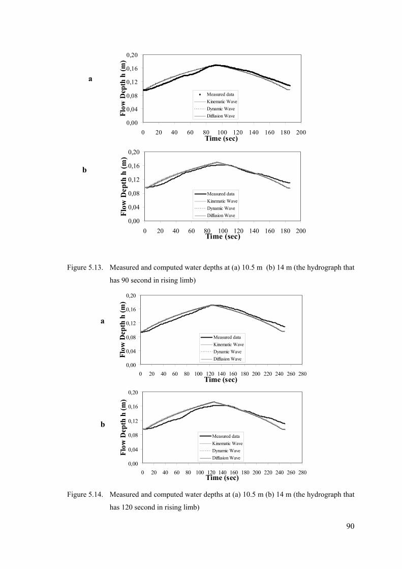
90

0,00

0,04

0,08

0,12

0,16

0,20

0 20 40 60 80 100 120 140 160 180 200Time (sec)

Flow

Dep

th h

(m)

Measured dataKinematic WaveDynamic WaveDiffusion Wave

0,00

0,04

0,08

0,12

0,16

0,20

0 20 40 60 80 100 120 140 160 180 200Time (sec)

Flow

Dep

th h

(m)

Measured dataKinematic WaveDynamic WaveDiffusion Wave

Figure 5.13. Measured and computed water depths at (a) 10.5 m (b) 14 m (the hydrograph that

has 90 second in rising limb)

0,00

0,04

0,08

0,12

0,16

0,20

0 20 40 60 80 100 120 140 160 180 200 220 240 260 280Time (sec)

Flow

Dep

th h

(m)

Measured dataKinematic WaveDynamic WaveDiffusion Wave

0,00

0,04

0,08

0,12

0,16

0,20

0 20 40 60 80 100 120 140 160 180 200 220 240 260 280Time (sec)

Flow

Dep

th h

(m)

Measured dataKinematic WaveDynamic WaveDiffusion Wave

Figure 5.14. Measured and computed water depths at (a) 10.5 m (b) 14 m (the hydrograph that

has 120 second in rising limb)

a

a

b

b

91

The overall computed error measures for simulations are presented in Table 5.1.

As seen, the mean relative error of 2.5=MRE implies that the developed model makes

about 5% error in predictions. The computed values of RMSE (root mean square error)

and MAE are 0.007 and 0.006 cm, respectively.

Table 5.1. Computed RMSE , MAE , MRE

Kinematic W. Dynamic W. Diffusion W.0,0074 0,0072 0,0073

Kinematic W. Dynamic W. Diffusion W.0,0065 0,0064 0,0064

Kinematic W. Dynamic W. Diffusion W.5,1952 5,0646 5,0789

RMSE, cm

MAE, cm

MRE, %

5.1.3.4.2. Test II

The second test was against the experimental data of aggradation depths

measured by Soni (1981a) in a laboratory flume of rectangular cross section. The flume

used by Soni was 30.0 m long, 0.20 m wide and 0.50 m deep. In the experimental run

constant equilibrium flow discharge was smQ /02.0 3= and uniform flow depth

was mh 092.00 = . The sand used for bed material and sediment feed in the experiments

had a median diameter of mmd s 32.0= and specific gravity of 2.65. Soni performed

experiments in the mobile bed condition to better represent natural rivers. Initially the

flume was filled with sand to a depth of 15 cm. Then the rectangular flume was filled

slowly with water and control valve was used to attain the specified discharge. The tail

gate height was adjusted in a way so that uniform flow was obtained in the flume by

allowing the bed to adjust by erosion or deposition. A uniform flow condition in the

flume was achieved when the measured bed and water surface were parallel to each

other. After reaching the uniform flow condition, sediment was dropped at the upstream

of the flume at a constant rate. The sediment injection section was located far enough

from the entrance of the flume to avoid entrance disturbances. The aggradation in the

bed started due to the excess load of the sediment. Bed and water surface elevation were

measured at regular time intervals (from 10 to 20 min at eleven sections). Aggradation

92

runs were continued until the end point of the transient profiles reached the downstream

end.

For computing the maximum bed elevation maxz , Langbein and Leopold (1968)’s

given a value of 2max /245 mkgCb = . The porosity was assumed to be 4.0=p . The flow

was uniform and steady and suspended sediment was negligible in this experiment, so

Equation 5.2 would suffice to model the bed aggradation.

Time : 30 min; Δqs=0.9qs

545658606264666870

0 2 4 6 8 10 12 14 16 18 20 22 24 26Distance (m)

Bed

leve

l (cm

)

Measured DataKinematic WaveEquilibrium bed profile

Time : 60 min; Δqs=0.9qs

545658606264666870

0 2 4 6 8 10 12 14 16 18 20 22 24 26Distance (m)

Bed

leve

l (cm

)

Measured DataKinematic WaveEquilibrium bed profile

Time : 90 min; Δqs=0.9qs

545658606264666870

0 2 4 6 8 10 12 14 16 18 20 22 24 26Distance (m)

Bed

leve

l (cm

)

Measured DataKinematic WaveEquilibrium bed profile

Figure 5.15. Simulation of measured bed profile at (a) 30 min (b) 60 min (c) 90 min

Figures 5.15a-5.15c show, respectively, simulations of bed profiles measured at

30, 60 and 90 min during the experimental run. The equilibrium flow conditions are

smQ /02.0 3= (equilibrium flow discharge), smqseq /10111 26−×= (equilibrium

a

b

c

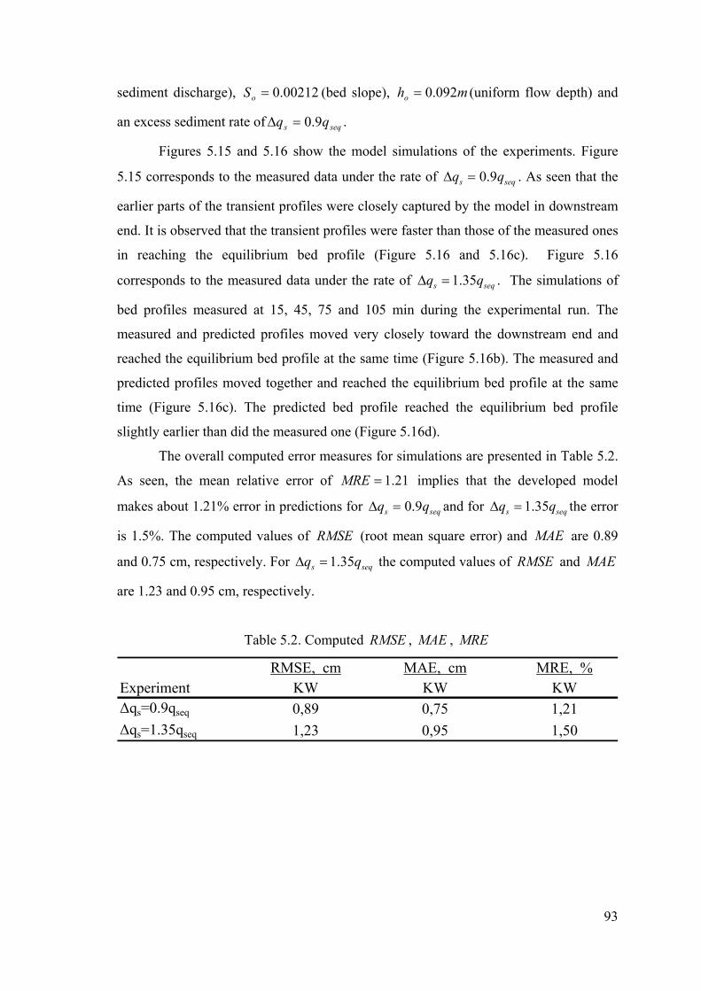
93

sediment discharge), 00212.0=oS (bed slope), mho 092.0= (uniform flow depth) and

an excess sediment rate of seqs qq 9.0=Δ .

Figures 5.15 and 5.16 show the model simulations of the experiments. Figure

5.15 corresponds to the measured data under the rate of seqs qq 9.0=Δ . As seen that the

earlier parts of the transient profiles were closely captured by the model in downstream

end. It is observed that the transient profiles were faster than those of the measured ones

in reaching the equilibrium bed profile (Figure 5.16 and 5.16c). Figure 5.16

corresponds to the measured data under the rate of seqs qq 35.1=Δ . The simulations of

bed profiles measured at 15, 45, 75 and 105 min during the experimental run. The

measured and predicted profiles moved very closely toward the downstream end and

reached the equilibrium bed profile at the same time (Figure 5.16b). The measured and

predicted profiles moved together and reached the equilibrium bed profile at the same

time (Figure 5.16c). The predicted bed profile reached the equilibrium bed profile

slightly earlier than did the measured one (Figure 5.16d).

The overall computed error measures for simulations are presented in Table 5.2.

As seen, the mean relative error of 21.1=MRE implies that the developed model

makes about 1.21% error in predictions for seqs qq 9.0=Δ and for seqs qq 35.1=Δ the error

is 1.5%. The computed values of RMSE (root mean square error) and MAE are 0.89

and 0.75 cm, respectively. For seqs qq 35.1=Δ the computed values of RMSE and MAE

are 1.23 and 0.95 cm, respectively.

Table 5.2. Computed RMSE , MAE , MRE

RMSE, cm MAE, cm MRE, %Experiment KW KW KWΔqs=0.9qseq 0,89 0,75 1,21Δqs=1.35qseq 1,23 0,95 1,50

94

Time : 15 min; Δqs=1.35qs

545658606264666870

0 2 4 6 8 10 12 14 16 18 20 22 24Distance (m)

Bed

leve

l (cm

)Measured DataKinematic WaveEquilibrium bed profile

Time : 45 min; Δqs=1.35qs

545658606264666870

0 2 4 6 8 10 12 14 16 18 20 22 24Distance (m)

Bed

leve

l (cm

)

Measured DataKinematic WaveEquilibrium bed profile

Time : 75 min; Δqs=1.35qs

545658606264666870

0 2 4 6 8 10 12 14 16 18 20 22 24Distance (m)

Bed

leve

l (cm

)

Measured DataKinematic WaveEquilibrium bed profile

Time : 105 min; Δqs=1.35qs

545658606264666870

0 2 4 6 8 10 12 14 16 18 20 22 24Distance (m)

Bed

leve

l (cm

)

Measured DataKinematic WaveEquilibrium bed profile

Figure 5.16. Simulation of measured bed profile at (a) 15 min (b) 45 min (c) 75 min (d) 105

min

a

b

c

d

95

5.2. One Dimensional Numerical Model for Sediment Transport under

Unsteady and Nonequilibrium Conditions

All the sediment transport functions or equations presented earlier have been

intended for the estimation of bed levels at the equilibrium condition with no scour or

deposition, at least from a statistical point of view. It has been assumed that the amount

of wash load depends on the supply from upstream and is not a function of the hydraulic

conditions at a given station. Also, the amount of wash load is not high enough to

significantly affect the fall velocity of sediment particles, flow viscosity or flow

characteristics in a river in comparison with these values in clear water. When the wash

load or concentration of fine material is high, non equilibrium bed material sediment

transport may occur.

The floods may cause heavy erosion and landslides in a river basin causing

sediment overloading within a river reach. During the aggradation and degradation,

there may be an exchange of sediment particles between bed layer and suspended layer

exceeding the flow capacity. The nonequilibrium sediment transport condition results in

an unstable streambed elevation. In such cases a numerical sediment transport model

provides the computational framework for analysis.

There are significant differences between the calculations of equilibrium and

nonequilibrium conditions. The nonequilibrium condition solution can be obtained by

numerical sediment modeling using control volume approach.

5.2.1. Governing Equations

Tayfur and Singh (2007) studied transport movement in a wide rectangular

alluvial channels represented in two layers. Figure 5.17 shows the possible exchange of

sediment between two layers: the water flow layer and movable bed layer, depending

upon flow transport capacity and sediment rate in suspension.

96

Figure 5.17. Definition Sketch of two layer system in nonequilibrium condition

(Source: Tayfur and Singh 2007)

The water flow layer may contain suspended sediment. The movable bed layer

consists of both water and sediment particles; therefore bed layer includes porosity

(Tayfur and Singh 2007). Equations 5.1 and 5.2 are for equilibrium conditions, where

the entrainment rate ( zE ) is equal to the deposition rate ( cD ) ( cz DEei =.,. ). Under

nonequilibrium condition entrainment rate is not equal to the deposition rate ( cz DE ≠ ).

This makes the solution more complex than equilibrium approach. Pianese (1994)

employed one more equation, adaptation equation relating the change in bed level in

time to flow variables ( hu, ) , equilibrium suspended sediment concentration ( eqc ) and

suspended sediment concentration ( c ) to simplifing the solution. The adaptation

equation is,

( )ccuhtzp eq −=∂∂

−λ

)1( (5.52)

where,

λ =adaptation length

If the right hand side of the equation is negative, it represents detachment rate, if

it is positive, it represents deposition rate (Pianese 1994). When deposition occurs, z

increases, but c decreases. Otherwise, when detachment occurs, z decreases, c increases.

Mohammadian et al. (2004) employed an equation for the conservation of water

z

h Ez Dc

97

(Equation 5.1) (assuming clear water 0=c ) and an equation for conservation of

suspended sediment in the water flow layer as:

( )ccv

xchV

xxhuc

thc

eqf

x −+⎟⎠⎞

⎜⎝⎛

∂∂

∂∂

=∂∂

+∂∂

η (5.53)

where,

xV = the sediment mixing coefficient

η = a coefficient

As explained before, the right side of the equation represents deposition

(negative) or detachment rate (positive). They also used an additional equation which

represents the change in bed level in time to the particle fall velocity, equilibrium

suspended sediment concentration ( )eqc , and suspended sediment concentration ( )c as:

( ) ( )ccv

tzp eq

f −=∂∂

−η

1 (5.54)

There are some deficiencies in Equations 5.53 and 5.54. One of them is that

when the last term on the right hand side of the Equation 5.53 is negative, it acts a sink

of concentration in the bed layer, so there should be a negative sign in front of the term

on the right hand side of the equation. The second deficiency is concern with Equation

5.54. It does not fully represent the conservation of mass equation for the sediment in

the movable bed layer, since it ignores the major term of the sediment flux gradient

⎟⎠⎞

⎜⎝⎛∂∂

xqbs . Mohammadian et al. (2004) who did not employ Equation 5.2, ignored the bed

sediment flux term. To avoid any confusion, the conservation of mass for suspended

sediment in the water flow layer and the conservation of mass for bed sediment in the

movable bed layer are written separately (Tayfur and Singh 2007);

[ ]czs

sus DEqx

huct

hc−+=

∂∂

+∂∂

ρ1

1 (5.55)

98

( ) [ ]zcs

bedbs EDqx

qtzp −+=

∂∂

+∂∂

−ρ11 1 (5.56)

where,

susq1 = the lateral suspended sediment (L/T)

bedq1 =the lateral bed load sediment (L/T)

sρ = the sediment mass density (M/L3)

zE = the detachment rate (M/L2/T)

cD = the deposition rate (M/L2/T)

The equations include the exchange of sediment due to the detachment and

deposition between the two layers. The process is cz DE ≠ in the non equilibrium

condition. The process is cz DE = in the equilibrium condition. When cz DE > , there is

entrainment from the bed layer (reducing the bed elevation, increasing the suspended

sediment concentration). When cz DE < , there is deposition from the bed layer

(increasing the bed elevation, reducing the suspended sediment concentration).

According the Equations 5.1, 5.55 and 5.56, there are five unknowns, zcuh ,,,

and bsq . Therefore, two more equations are needed for solving the system. One more

equation can be obtained from the momentum equation for water flow. In this study, the

kinematic wave approximation was employed for the momentum equation (Equation

5.4). The fifth equation can be obtained by relating sediment transport rate to sediment

concentration in the movable bed layer. In this study, the kinematic theory was

employed (Tayfur and Singh 2006) (Equation 3.69).

Combining the Equations 3.69, 5.1, 5.4, 5.55 and 5.56 can be written in a

compact form as:

( ) ( ) ( ) ( )cq

xc

ch

tc

ch

tz

cp

xhh

th w

−=

∂∂

−−

∂∂

−−

∂∂

−+

∂∂

+∂∂ −

111111

ββ ααβ (5.57)

[ ]czs

sus DEhh

qxhhc

th

hc

xch

tc

−+=∂∂

−∂∂

+∂∂

+∂∂ −−

ραβα ββ 1121 (5.58)

99

( ) ( ) [ ]zcs

beds ED

ppq

xz

zzv

tz

−−

+−

=∂∂

⎥⎦

⎤⎢⎣

⎡−+

∂∂

11

121 1

max ρ (5.59)

These equations are kinematic wave equations for modeling unsteady state,

nonuniform transient channel bed profiles under nonequilibrium conditions. For

calculating the detachment rate zE , the shear stress approach was used (Yang 1996);

( )[ ]kcrcz TE ττσσ −Φ== (5.60)

where,

owhSγτ = (5.61)

( ) swscr dγγκτ −= (5.62)

where,

σ =the transfer rate coefficient (1/L)

cT = the flow transport capacity (M/L/T)

Φ = the soil erodibility coefficient

τ = the shear stress (M/L2)

crτ = the critical shear stress (M/L2)

k = an exponent

sw γγ , = the specific weight of water and sediment respectively (M/L3)

κ = a constant

sd = the sediment particle diameter (L)

The deposition rate cD can be expressed as (Yang 1996);

[ ]hucqD ssssc ρσσρ == (5.63)

where,

ssq = the unit suspended sediment discharge (M/L/T)

100

5.2.1.1. Numerical Solution of Kinematic Wave Equations

Equations 5.57, 5.58 and 5.59 were solved using the finite difference scheme

developed by Lax (1954) as explained before (Equations 5.14 and 5.15). Note that the

finite difference equations were written for both the layers not only at the central nodes

of the domain but also at the downstream nodes. All the equations were solved

simultaneously for each time step. The finite difference equations are:

( ) ( ) ( ) ( )[ ]

( ) ( )[ ] ( )( ) ( )ji

wji

jij

i

ijji

ji

jij

i

ji

ji

ji

jij

i

ji

jiij

ji

ji

ji

ctqcc

ch

xtccc

ch

zzzc

phhhx

thhh

−Δ

+−−Δ

Δ++−

−+

+−−

−−Δ

Δ−+=

−+−++

−++

−+−

−++

1125.0

1

5.012

5.0

11111

1

111

111

111

β

β

α

αβ

(5.64)

( ) ( ) ( )[ ]

( ) [ ]ijc

ijzj

isj

i

susji

jiij

ji

ji

ji

jij

i

jij

ij

iijj

ij

ij

i

DEht

htqhhhc

xt

hhhhccch

xtccc

−Δ

+Δ

+−Δ

Δ−

+−−−ΔΔ

−+=

−+−

−++

−+−

−++

ραβ

α

β

β

111

2

111

111

111

2

5.02

5.0 (5.65)

( ) ( ) ( ) ( ) [ ]ijz

ijc

s

susji

ji

jisj

ij

ij

i EDp

tptqzz

zz

xtvzzz −

−Δ

+−Δ

+−⎟⎟⎠

⎞⎜⎜⎝

⎛−

ΔΔ

−+= −+−++

1121

25.0 1

11max

111

ρ (5.66)

where,

i = stands for space node

j = stands for time node

tΔ = time increment

xΔ =space increment

By using presented algorithm, the unknown values of ch, and z at the new time

level 1+j (future time) are determined at every interior node ( i = 2,….N-1). The values

of the dependent variables ch, and z at the boundary nodes 1 and N+1 are determined

by using boundary conditions. Also, at the time level j =1, initial conditions are already

known (Figure 5.2)

101

Initial conditions can be specified as:

( ) ohxh =0, (5.67)

( ) ocxc =0, (5.68)

( ) ozxz =0, (5.69)

where,

oo ch , and oz = the initial flow depth (L), concentration (L3/L3) and the bed level (L),

respectively.

The upstream boundary conditions can be specified as inflow hydrograph and

inflow sedimentograph.

( ) )(,0 thth = 0.0>t (5.70)

( ) )(,0 tctc = 0.0>t (5.71)

( ) )(,0 tztz = 0.0>t (5.72)

The downstream boundary conditions can be specified as:

( ) 0),(=

∂∂

xtNh ( 1

111

+−

++ = j

Nj

N hh ) 0.0>t (5.73)

( ) 0),(=

∂∂

xtNc ( 1

111

+−

++ = j

NjN cc ) 0.0>t (5.74)

( ) 0),(=

∂∂

xtNz ( 1

111

+−

++ = j

NjN zz ) 0.0>t (5.75)

102

●Stability

The numerical scheme has to satisfy the stability conditions. For this reason, the

Courant – Friedrichs – Lewy (CFL) condition was used. Since the water waves travel at

a much higher velocity than the bed transients this condition is given as before Equation

5.24.

Equations 5.64, 5.65 and 5.66 are solved simultaneously for each time step.

5.2.1.2. Model Application

The channel was assumed to have a 1000 m length and 30 m width with 0.0015

bed slope. The model parameters basically are as follows:

PCSFkzSpC ssoz ,,,,,,,,,,, max κφσγρ Φ and sd . Parameters sρ , sγ , and sd can be obtained

from experimental sediment data. Chezy roughness coefficient is assumed to be

smCz /36 5.0= . The sediment was assumed to have 3/2650 mkgs =ρ , mmds 32.0=

and 528.0=p . Maximum concentration was assumed 2max /500 mkgC = (note that

( ) spCz ρ−= 1maxmax ). Gessler (1965) suggested a value of 0.047 for κ for most flow

conditions. The value of transfer rate can be calculated in flumes by ( )h71=σ , where

h is flow depth, parameter Φ has a range of 0.0 – 1.0 and exponent ik has a range of 1.0

– 2.5 in literature (Foster 1982, Tayfur 2002, Yang 1996). The inflow hydrograph and

inflow concentration were given in Figure 5.18 for upstream boundary conditions.

103

0

20

40

60

80

100

120

140

0 30 60 90 120 150 180 210 240Time (min)

Q (m3/s)

0102030405060708090

0 30 60 90 120 150 180 210 240Time (min)

C (kg/m2)

Figure 5.18 (a) Inflow hydrograph. (b) Inflow concentration

Figures 5.19a-5.19d present bed profiles during the rising limp, equilibrium,

recession limb and postrecession limp of the inflow hydrograph and concentration,

respectively. It is seen that while inflow concentration increases, the bed level gradually

increases in upstream and it decreases after about 200 m in the downstream (Figure

5.19a). The bed elevation continues to increase in the equilibrium period at the upstream

end (Figure 5.19b). In rising period the bed level reaches at equilibrium after the 200 m

of the channel (Figure 5.21c). In procession period the bed level nearly same afert the

200 m (Figure 5.19d).

a

b

104

0

0,1

0,2

0,3

0,4

0,5

0 100 200 300 400 500 600 700 800 900 1000

Distance (m)

Bed

ele

vatio

n z

(m) 20 min

40 min60 min

0

0,1

0,2

0,3

0,4

0,5

0,6

0 100 200 300 400 500 600 700 800 900 1000

Distance (m)

Bed

ele

vatio

n z

(m)

80 min100 min

0

0,2

0,4

0,6

0,8

1

0 100 200 300 400 500 600 700 800 900 1000

Distance (m)

Bed

ele

vatio

n z

(m)

140 min160 min

0

0,2

0,4

0,6

0,8

1

0 200 400 600 800 1000

Distance (m)

Bed

ele

vatio

n z

(m)

180 min220 min240 min

Figure 5.19. Transient bed profile at (a) rising period (b) equilibrium period (c) recession

period (d) post recession period of inflow hydrograph and concentration

a

b

c

d

105

5.2.1.3. Model Testing Using Experimental Data

The model was tested against the experimental data of aggradation depths

measured by Yen et al. (1992) in laboratory flume. The flume used for present

experiments is 72 m long and 1 m wide. The water discharge was maintained at a

constant rate of sm /12.0 3 for all experiments. The initial bed slope is 0.0035 and

sediment median diameter is 1.8 mm. At the beginning of an experiment, a sediment

supply rate of 3.3 kg/min (dry mass) was continuously released from the upstream end

until the channel bed reached a state of equilibrium. The sediment supply rate was then

increased to 9.9 kg/min until a new equilibrium was reached. The rate of sediment

supply was thereafter reduced back to and kept at 3.3 kg/min until another new

equilibrium was reached. Finally, the sediment supply was cut off, and only clear water

was released from the upstream end until the channel bed was fully armored. Each

period lasted for about 30 hours. Bed elevations were measured 5 m apart from each

other. A sluice gate at the downstream end of the flume was employed to maintain a

constant tailwater level. The details of the experiment can be obtained from Yen et al.

(1992).

Simulations of bed profiles measured at 30, 60, 90 and 120 hours during the

experiment run (Figure 5.20.). The model and measured data nearly closed at each

location along the bed. At 120 hr predicted and measured data were nearly same (Figure

5.20d).

106

Time : 30 hr

2022242628303234

0 5 10 15 20 25Distance (m)

Bed

Ele

vatio

n z

(cm

) PredictedMeasuredOriginal Bed

Time : 60 hr

20

24

28

32

36

40

0 5 10 15 20 25Distance (m)

Bed

Ele

vatio

n z

(cm

) PredictedMeasuredOriginal Bed

Time : 90 hr

20222426

28303234

0 5 10 15 20 25Distance (m)

Bed

Ele

vatio

n z

(cm

) PredictedMeasuredOriginal Bed

Time : 120 hr

2022

24262830

3234

0 5 10 15 20 25Distance (m)

Bed

Ele

vatio

n z

(cm

) PredictedMeasuredOriginal Bed

Figure 5.20. Simulation of bed profiles along a channel bed at (a) 30 h, (b) 60 h, (c) 90

h and (d) 120 h of the laboratory experiment

a

b

c

d

107

Figure 5.21 presents simulation of bed level measured at 10 m away from the

upstream end during the experiment period of 120 hours. The model simulations of

transient bed levels at the specified locations are satisfactory. The model closely

predicted bed levels during, rising equilibrium and recession periods satisfactory.

The overall computed error measures for simulations are presented in Table 5.3

Location #1. As seen, the mean relative error of 99.1=MRE implies that the developed

model makes about 1.99% error in predictions. The computed values of RMSE (root

mean square error) and MAE are 0.82 and 0.66 cm, respectively.

Table 5.3. Computed RMSE , MAE , MRE

RMS, cm MAE, cm MRE, %0,820 0,663 1,992

Location #1

28

30

32

34

36

38

40

0 20 40 60 80 100 120

Time (hr)

Bed

Ele

vatio

n z

(cm

) PredictedMeasured

Figure 5.21. Simulation of bed profiles in time during the laboratory experiment at six

different locations of the experimental channel. Location #1 is 10 m away from

the upstream end (Yen, et al. 1992)

5.2.1.4. Model Testing: Comparing the Equilibrium and

Nonequilibrium models for Hypothetical Cases

The hypothetical cases were analyzed assuming inflow concentration

hydrograph at the upstream of the channel as shown in Figures 5.22. The channel was

assumed a flume and to have a 20 m length and 1 m width with 0.0001 bed slope. The

sediment was assumed to have 2650=sρ kg/m3, 09.0=sd mm, 45.0=p and sediment

transport capacity coefficient 000075.0=κ (Ching and Cheng 1964). Langbein and

108

Leopold (1968) suggest 500max =C kg/m2 (note that sb zpC ρ)1( −= ). The water

discharge is 5.0=Q sm /3 at the beginning. In equilibrium part smQ /1 3= (in

trapezoidal).

For two model solutions a Courant number was selected 0.2. The numerical

solutions are plotted mx 500= along the channel (Figure 5.23). It is seen that the

different behavior of equilibrium and nonequilibrium model, particularly at peak flow

points. The equilibrium model reaches faster to maximum flow rate. On the other hand,

the nonequilibrium model has a smaller peak. It can be said that bed material decreases

because of suspended sediment increases.

0,4

0,6

0,8

1

1,2

1,4

0 40 80 120 160 200 240

Time (min)

C (kg/m2)

Figure 5.22. (a) Inflow hydrograph. (b) Inflow concentration

Comparison Equilibrium and Nonequilibrium Model

0,02

0,03

0,04

0,05

0,06

0,07

0,08

0,09

0,1

0 40 80 120 160 200 240

Time (min)

Bed

Lev

el z

(m)

nonequilibrium model equilibrium model

Figure 5.23. Comparing the equilibrium and nonequilibrium models

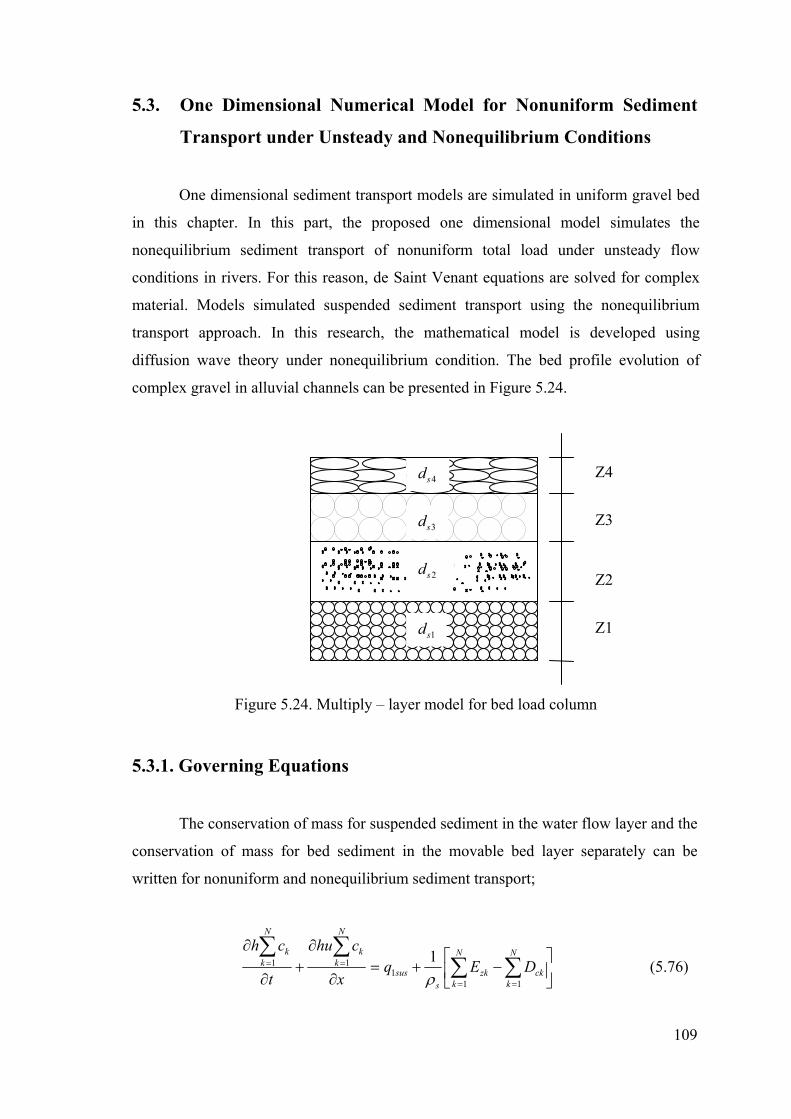
109

5.3. One Dimensional Numerical Model for Nonuniform Sediment

Transport under Unsteady and Nonequilibrium Conditions

One dimensional sediment transport models are simulated in uniform gravel bed

in this chapter. In this part, the proposed one dimensional model simulates the

nonequilibrium sediment transport of nonuniform total load under unsteady flow

conditions in rivers. For this reason, de Saint Venant equations are solved for complex

material. Models simulated suspended sediment transport using the nonequilibrium

transport approach. In this research, the mathematical model is developed using

diffusion wave theory under nonequilibrium condition. The bed profile evolution of

complex gravel in alluvial channels can be presented in Figure 5.24.

Figure 5.24. Multiply – layer model for bed load column

5.3.1. Governing Equations

The conservation of mass for suspended sediment in the water flow layer and the

conservation of mass for bed sediment in the movable bed layer separately can be

written for nonuniform and nonequilibrium sediment transport;

⎥⎦

⎤⎢⎣

⎡−+=

∂

∂+

∂

∂

∑∑∑∑

==

==N

kck

N

kzk

ssus

N

kk

N

kk

DEqx

chu

t

ch

111

11 1ρ

(5.76)

1sd

2sd

4sd

Z1

Z2

Z3

Z4

3sd

110

⎥⎦

⎤⎢⎣

⎡−+=

∂

∂+⎟

⎠⎞

⎜⎝⎛∂∂

⎟⎠

⎞⎜⎝

⎛− ∑∑

∑∑∑

==

=

==

N

kzk

N

kck

sbed

N

kbskN

k k

bN

kk EDq

x

q

tzp

111

1

11

11ρ

(5.77)

where,

kc = section – averaged sediment concentration of size class k

zkE = the detachment rate of size class k ( )TLM // 2

ckD = the deposition rate of size class k ( )TLM // 2

bskq = the sediment flux in the movable bed layer of size class k ( )TL /2

( )kb tz ∂∂ = bed change rate corresponding to the k th size class of sediment

kp = bed material porosity of size class k

5.3.1.1. Numerical Solutions of Nonuniform Model

Equations 5.40, 5.41, 5.76 and 5,77 were solved using the finite difference

scheme developed by Lax (1954) as explained before (Equations 5.14 and 5.15). The

finite difference equations are:

( )x

zz

xhhSS

N

kk

ji

N

kk

jij

ij

io

jfi Δ

⎟⎠

⎞⎜⎝

⎛−

−Δ−

−=∑∑=

−=

+−+

2

)()(

21

11

111 (5.78)

( ) ( )

⎟⎠

⎞⎜⎝

⎛−

Δ+⎟

⎠

⎞⎜⎝

⎛−

⎟⎠

⎞⎜⎝

⎛−

ΔΔ

+

⎥⎦

⎤⎢⎣

⎡⎟⎠

⎞⎜⎝

⎛+−

⎟⎠

⎞⎜⎝

⎛−

+

⎥⎦

⎤⎢⎣

⎡⎟⎠

⎞⎜⎝

⎛+−

⎟⎠

⎞⎜⎝

⎛−

−

−Δ

Δ−+=

∑∑∑

∑

∑∑∑∑

∑∑∑∑

=

=−

=+

=

=−

=+

=

+

=

=−

=+

=

+

=

−+−

−++

N

k

ji

wN

k

ji

N

k

jiN

k

ji

ij

N

k

ji

N

k

ji

N

k

jiN

k

ji

ji

N

k

ji

N

k

ji

N

k

jiN

k

ji

ji

jiij

ji

ji

ji

c

tqccc

hx

t

cccc

h

zzzc

p

hhhx

thhh

1

1

11

11

1

11

11

1

1

1

11

11

1

1

1

111

111

112

5.01

5.01

25.0

β

β

α

αβ

(5.79)

111

( ) ( )

( )[ ]

( )

[ ]kijck

ijzj

iksj

i

sus

ji

jiijk

ji

ji

ji

jij

i

kj

i

kj

ikj

iijkj

ikj

ikj

i

DEh

th

tq

hhhcx

t

hhhhc

cchx

tccc

)()()(

)(2

5.0)(

)()(2

)()(5.0

1

112

111

111

111

−Δ

+Δ

+

−Δ

Δ−

+−−

−ΔΔ

−+=

−+−

−++

−+−

−++

ρ

αβ

α

β

β

(5.80)

( ) ( )

( ) ( ) [ ]kijzk

ijc

kksk

sus

kj

ikj

ik

kj

iksk

jik

jik

ji

EDp

tp

tq

zzz

zx

vtzzz

)()(1)(1

)()()()(21

2)()()(5.0

1

11max

111

−−

Δ+

−Δ

+

−⎟⎟⎠

⎞⎜⎜⎝

⎛−

ΔΔ

−+= −+−++

ρ

(5.81)

By using the presented algorithm, the unknown values of h and z at the new

time level 1+j (future time) are determined from every interior node ( i = 2,…….,N-1).

The values of the dependent variables h and z at the boundary nodes 1 and N+1 are

determined by using boundary conditions. Also, at the time level j =1, initial conditions

are already known.

Initial and boundary conditions were specified before Equations 5.18 – 5.23.

And for stability the Courant – Friedrichs – Lewy (CFL) condition was used.

Equations 5.49, 5.50 and 5.51 are solved simultaneously for each time step.

5.3.1.2. Model Application

The channel assumed as a flume has 20 m length and 1 m width with 0.0005 bed

slope. The model parameters basically are as follows:

PCSFkzSpC ssoz ,,,,,,,,,,, max κφσγρ Φ and sd . Parameters sρ , sγ , and sd can be obtained

from experimental sediment data. Chezy roughness coefficient is assumed to be

smCz /50 5.0= . It is assumed that there are four different sediment types in the sediment

column. Sediment characteristics that used in the model are summarized in Table 5.4.

112

Table 5.4. Sediment Characteristics

type ρs (kg/m3) ds (mm) p 1 2700 0.5 0.40 2 2650 0.7 0.45 3 2600 0.9 0.55 4 2500 1.2 0.60

Maximum concentration 2max /500 mkgC = was assumed for each particle sizes

(note that ( ) spCz ρ−= 1maxmax ). Gessler (1965) suggested a value of 0.047 for κ for

most flow conditions. The value of transfer rate can be calculated in flumes

by ( )h71=σ , where h is flow depth, parameter Φ has a range of 0.0 – 1.0 and

exponent ik has a range of 1.0 – 2.5 in literature (Foster 1982, Tayfur 2002, Yang

1996). The inflow hydrograph and inflow concentration were given in Figure 5.25 for

upstream boundary conditions.

1,3

1,5

1,7

1,9

2,1

2,3

2,5

0 50 100 150 200 Time (min)

Q (m3/s)

40

50

60

70

80

90

100

110

0 50 100 150 200 Time (min)

C (kg/m2)

Figure 5.25 (a) Inflow hydrograph. (b) Inflow concentration

a

b

113

40 min

0,10,20,30,40,50,60,70,80,9

1

0 1 2 3 4 5 6 7 8 9 10 11 12 13 14 15 16 17 18 19 20

Distance (m)

Bed

Lev

el z

(m)

nonuniformmedian diameter

100 min

0,10,20,30,40,50,60,70,80,9

1

0 1 2 3 4 5 6 7 8 9 10 11 12 13 14 15 16 17 18 19 20

Distance (m)

Bed

Lev

el z

(m)

nonuniformmedian diameter

160 min

0,10,2

0,30,40,5

0,60,70,8

0,91

0 1 2 3 4 5 6 7 8 9 10 11 12 13 14 15 16 17 18 19 20

Distance (m)

Bed

Lev

el z

(m)

nonuniformmedian diameter

240 min

0,10,20,3

0,40,50,60,7

0,80,9

1

0 1 2 3 4 5 6 7 8 9 10 11 12 13 14 15 16 17 18 19 20Distance (m)

Bed

Lev

el z

(m)

nonuniformmedian diameter

Figure 5.26. Transient bed profiles of nonuniform sediment and uniform sediment model at (a)

rising period (b) equilibrium period (c) recession period (d) post recession period

of inflow hydrograph and concentration in unsteady flow conditions

a

b

c

d

114

Simulations were significantly under 50d (median diameter) and nonuniform

mixture for all the periods of the simulations. Under 50d (median diameter) conditions,

bed levels were lower than nonuniform flow case (Figure 5.26).

In another simulation for the same flume we considered constant inflow

hydrograph with smQ /2.1 3= and the same inflow sedimentograph seen in Figure

5.25.b. The simulations for the case are presented in Figure 5.27. While nonuniform

and uniform sediment transport model give similar performance under steady flow

condition, give different performance under unsteady flow conditions (Figure 5.27).

40 min

0,10,20,30,40,50,60,70,80,9

1

0 1 2 3 4 5 6 7 8 9 10 11 12 13 14 15 16 17 18 19 20

Distance (m)

Bed

Lev

el z

(m)

nonuniformmedian diameter

100 min

0,1

0,2

0,30,4

0,5

0,6

0,70,8

0,9

1

0 1 2 3 4 5 6 7 8 9 10 11 12 13 14 15 16 17 18 19 20Distance (m)

Bed

Lev

el z

(m)

nonuniformmedian diameter

Figure 5.27. Transient bed profiles of nonuniform sediment and uniform sediment model at (a)

rising period (b) equilibrium period (c) recession period (d) post recession period

of inflow hydrograph and concentration in steady flow conditions

(cont. on next page)

a

b

115

160 min

0,1

0,20,3

0,4

0,50,6

0,7

0,80,9

1

0 1 2 3 4 5 6 7 8 9 10 11 12 13 14 15 16 17 18 19 20Distance (m)

Bed

Lev

el z

(m)

nonuniformmedian diameter

240 min

0,1

0,20,3

0,4

0,50,6

0,7

0,80,9

1

0 1 2 3 4 5 6 7 8 9 10 11 12 13 14 15 16 17 18 19 20Distance (m)

Bed

Lev

el z

(m)

nonuniformmedian diameter

Figure 5.27. (cont.) Transient bed profiles of nonuniform sediment and uniform sediment

model at (a) rising period (b) equilibrium period (c) recession period (d) post

recession period of inflow hydrograph and concentration in steady flow

conditions

c

d

116

CHAPTER 6

SUMMARY AND CONCLUSION

6.1. Summary

Three mathematical and numerical models have been developed under

kinematic, diffusion and dynamic wave approaches for simulating bed profiles in

alluvial channels under unsteady and equilibrium conditions. Transient bed profiles are

also simulated for several hypothetical cases, comparing different particle velocities and

different particle fall velocities. The model tested with flume experiments. Also

different wave models (kinematic, diffusion and dynamic) were compared. The

kinematic wave model was developed for simulating transient bed profiles in alluvial

channels under unsteady and nonequilibrium conditions and tested against experimental

data. The diffusion wave model was developed for simulating transient bed profiles in

alluvial channels under unsteady, nonuniform and nonequilibrium conditions.

6.2. Conclusion

1. Numerical model is able to capture the effects of suspended sediment and bed

load sediment on the transport. When the transport capacity is greater than the

suspended load, deposition occurs, otherwise detachment occurs. The model is

able to capture this phenomenon.

2. The application of the developed model to hypothetical cases revealed that the

model is able to capture the behavior of the process in alluvial channels.

3. Modeling the process under nonequilibrium conditions give different results

than those under equilibrium conditions. Therefore, if the flow conditions in

nonequilibrium, it should be so modeled.

4. The model was not tested against experimental data under unsteady and

nonequilibrium flow and sediment loadings. The next aim is to test the model for

that general case.

117

5. The selected on particle velocity, particle fall velocity and hydrodynamic wave

(kinematic, diffusion and dynamic) would be better decided with testing of the

model with the general case (unsteady, nonequilibrium) experimental data.

6. Another shortcoming is the application of the model is field conditions. This is

able one of the future plans.

7. The investigation of different particle velocity formulations revealed that under

the same flow conditions, wave front is faster in Kalinske and Bridge and

Dominic’s formulation.

8. The investigation of different particle fall velocity formulations revealed that

under the same flow conditions, they produced nearly the same results.

9. The investigation of the effect of maxz (maximum bed level) on the transport

revealed that it is an important parameter. It significantly affects the wavefront

speed and bed level. The higher the maxz , the faster the wavefront and the higher

the bed level.

10. The numerical investigation of different sediment flux (bed load) formulations

revealed that under the same transport flow condition, the kinematic wave theory

produced different results then Meyer – Peter and Schoklists. Meyer – Peter and

Schoklists produced nearly the same profiles. Under kinematic wave theory, the

wavefronts move faster.

11. The numerical comparison of kinematic, diffusion and dynamic wave for

hypothetical cases of sediment transport revealed under the same sediment flux

function of the wavefront is slower in the case of kinematic wave.

12. The hydrodynamic part the developed numerical model was tested successfully

tested experimental flume data. It satisfactorily (less then 5%) simulated the

measured data.

13. The developed numerical model was tested against measured sediment data

from the literature. It predicted measured bed levels satisfactorily.

14. The numerical model revealed that modeling sediment mixtures with only mean

particle diameter 50d approximation might lead to misleading results. In other

words, it’s better model with the mixture with corresponding particle

characteristics i.e. 50d (median diameter), sρ (density) and p (porosity).

118

REFERENCES

Ackers, P. and White, W. R. 1973. Sediment Transport: New Approach and Analysis.

Journal of the Hydraulics Division, ASCE 99: 2041-2060. Al-Khafif, S. M. 1965. Study of open channels degradation and corresponding bed

roughness. University of California. Thesis of PhD.. Bagnold, R. A. 1966. An approach to the sediment transport problem from general

physics. Geological survey prof. paper 422-I. Washington. D.C. Begin, Z. B., Meyer, D. F. and Schumm, S. A. 1981. Development of longitudinal

profiles of alluvial channels in response to base-level lowering. Earth Surface Processes and Land Forms 6(1): 49-68.

Bhallamudi, S. M. and Chaudhry, M. H. 1989. Numerical Modeling of Aggradation and

Degradation in Alluvial Rivers. Journal of Hydraulic Engineering 117(9). Bhamidipaty, S. and Shen, W. H. 1971. Laboratory Study of Degradation and

Aggradation. Journal of Waterways, Harbors and Coastal Engineering Division 97: 615- 630.

Blumberg, A. and Mellor, G. L. 1987. A description of A three-dimensional Coastal

Ocean Circulation Model. In Three-Dimensional Coastal Ocean Models. American Geophysical Union, N. S. Heaps (Ed.), 1-16, Washington, DC.

Boer, S., DeVriend, H. J. and Wind, H. G. 1984. A Mathematical Model for the

Simulation of Morphological Processes in the Coastal Area. Proc. 19th ICCE, Houston. USA: 1437-1453.

Bor, Aslı, Tayfur, G. and Elçi, Ş. 2008. Parçacık Hızı ve Düşüm Hızının Katı Madde

Taşınımına Etkisinin Kinematik Dalga Yaklaşımı ile Modellenmesi. Havza Kirliliği Konferansı. DSİ II. Bölge Müdürlüğü, Gümüldür, 2008, İzmir: 89-96.

Bor, A., Elçi, Ş. and Çalışkan A. 2008. Prediction of Sedimentation in Reservoirs by

Acoustic Methods. River Flow International Conference on Fluvial Hydraulics, Cesme, Izmir, Turkey. River flow 2008, 2: 1251-1260.

Bridge, J. S. and Dominic, D. F. 1984. Bed Load Grain Velocities and Sediment

Transport Rates. Water Resources Res. 20(4): 476-490. Cao, Z. and Egiashira, S. 1999. Coupled Mathematical Modelling of Alluvial Rivers.

Journal of Hydraulic Engineering 17(2): 71-85. Cao, Z., Day, R. and Egiashira, S. 2001. Coupled and Decoupled Numerical Modelling

of Flow and Morphological Evolution in Alluvial Rivers. Journal of Hydraulic Engineering, ASCE 128(3): 306-321.

119

Cao, Z. and Carling, P. A. 2003. On evolution of bed material waves in alluvial rivers, Earth Surf. Processes Landforms 28: 437-441.

Capart, H. 2000. Dam break induced geomorphic flows and the transition from solid to

fluid like behavior across evolving interfaces. Catholic University. Thesis of PhD.

Capart, H. and Young, D. L. 2002. Two Layer Shallow Water Computation of

Torrential Geomorphic Flows. River Flow International Conference on Fluvial Hydraulics, Louvain-la-Neuve, Belgium, River flow 2002, 2: 1003.

Casulli, V. 1990. Semi-Implicit Finite Difference Methods for the Two-dimensional Shallow Water Equations. J. Comput. Phys. 86: 56-74. Chang, F. M., Simons, D. B. and Richardson, E. V. 1965. Total Bed-Material Discharge

in Alluvial Channels. U.S. Geological Survey Water-Supply I: 1498. Chang, H. H. 1982. Mathematical Model for Erodible Channels. J. Hydraul. Div. Am.

Soc. Civ. Eng. 108(5): 678-689. Chaudhry, M. H. 1993. Open – Channel Flow. New Jersey: Prentice Hall, Englewood

Cliffs, 07632. Chaudhry, M. H. 1996. Principles of flow of water. Chapter 2 in Handbook of Water

Resources. L.Mays (ed.). McGraw-Hill. Chien, H. H. and Wan, Z. H. 1999. Mechanics of Sediment Transport. Am. Soc. of Civ.

Eng. Reston, Va. Ching, H. H. and Cheng, C. P. 1964. Study of River Bed Degradation and Aggradation

by The Method of Characteristics. Journal of Hydraulic Engineering 5: 41. Colby, B. R. and Hembree, C. H. 1955. Computation of total sediment discharge,

Niobrara River near Cody, Nebraska. Supply Paper 1357. U.S. Geological Survey, Water. Washington, D.C.

Collins, W., Gregory, R., Anderson, J. 1996. A digital approach to seabed

classification. Sea Technology 37(8): 83–87. Correia, L., Krishnappan, B. G. and Graf, W. H. 1992. Fully Couplad Unsteady Mobile

Boundary Flow Model (FCM). Journal of Hydraulic Engineering 118(3): 476-494.

Cui, Y., Parker, G. and Paola, C. 1996. Numerical Simulation of Aggradation and

Downstream Fining. Journal of Hydraulic Res. 34(2): 195-204. Cunge, J. A., Holly, F. M. and Verwey, A. 1980. Practical Aspects of Computational

River Hydraulics. Pitman, USA.

120

Cunge, J.A. and Perdreau, N. 1973. Mobile bed fluvial mathematical models. LaHouille Blanch. 7: 561-580.

Curran, J. C. and Wilcock, P. R. 2005. Effect of Sand Supply on Transport Rates in a

Gravel-bed Channel. Journal of Hydraulic Engineering 131(11): 961 – 967. Demuren, A. O. and Rodi, W. 1986. Calculation of Flow and Pollutant Dispersion in

Meandering Channels. Journal of fluid mechanics 172: 63-92, Cambridge, U.K. de Vries, M. 1965. Consideration About Non – Steady Bed Load Transport in Open

Channels. XI Congress, Int Assoc. of Hydraul. Eng. and Res. St. Petersburg, Russia.

de Vries, M. 1973. River Bed Variation – Aggradation and Degradation. Publ. 107,

Delft Hydaulic Lab. Delft, Netherlands. de Vries, M. 1975. A Morphological Time Scale for Rivers. XVI Congress, Int Assoc. of

Hydraul. Eng. and Res. Sao Paulo, Brazil. DHI Inc. 2003. MIKE21 user guide. http://www.dhisoftware.com/ 301 South State

Street, Newtown, PA, 18940, USA. Di Cristo, C., Leopardi, A. and Greco, M. 2002. A Bed-Load Transport Model for Non-

Uniform Flows. River Flow International Conference on Fluvial Hydraulics, Louvain-laNeuve, Belgium. River flow 2002, 2: 859.

Dietrich, W. E. 1982. Settling Velocity of Natural Particles. Water Resources Res.

18(6): 1615-1626. Duboys, M. P. 1879. Le Rhone et les Rivieres a Lit affouillable. Annales de Ponts et

Chausse, sec. 5, 18: 141-195. Dyer, K. 1986. Coastal and Estuarine Sediment Dynamics. John Wiley & Sons, Inc.,

New York. ECOMSED 2002. Users Manual. HydroQual Inc. Mahwaj N.J. Einstein, H. A. 1950. The Bed Load Function for Sediment Transportation in Open

Channel Flows. Technical Bulletin no. 1026, U.S. Department of Agriculture. Washington, D.C.

Engelund, F. and Hansen, E. 1972. A Monograph on Sediment Transport in Alluvial

Streams. Teknisk Forlag. Copenhagen. Foster, G. R. 1982. Modelling the erosion process in hydraulic modeling of small

Watersheds. edited by C. T. Haan, H. P. Johnson, and D. L. Brakensiek. Am. Soc. of. Agric. Eng. St. Joseph. Mich.

121

Gessler, J. 1965. The beginning of bed – load movement of mixtures investigated as natural armoring in channels. W. M. Keck Lab. of Hydraul. and Water Resour. Calif. Inst. of Tech. Pasedana, California.

Gill, M. A. 1983a. Diffusion Model for Aggrading Channels. Journal of Hydraulic

Research, IAHR 21(5): 355-367. Gill, M. A. 1983b. Diffusion Model for Degrading Channels. Journal of Hydraulic

Research, IAHR 21(5): 21:369-378. Gill, M. A. 1987. Nonlinear Solution of Aggradation and Degradation in Channels.

Journal of Hydraulic Research 25(5), 537-547. Guy, H.P., Simons, D.B., Richardson, E.V. 1966. Summary of alluvial channel data

from flume experiments. Professional Paper 462-I. United States Geological Society, Washington, D.C.

Güney, M. Ş. and Bombar, G. 2008. TÜBİTAK Araştırma Projesi Gelişme Raporu.

Proje no. 106M274, Rapor no. 4, Rapor dönem no. 4. Hamrick, J.M. 1996. Users manual for the environmental fluid dynamic computer code.

Virginia Institute of Marine Science. Special Report 328, 224. Hayter, E. j., Bergs, M. A., Gu, R., McCutcheon, S., Simth, S. J. and Whiteley, H. J.

1995. HSCTM- 2D. A finite element model for depth averaged hydrodynamics, sediment and contaminant transport.

Higginbottom, I., Hundley, A., Pauly, T. 1994. A Desktop Study of Some Acoustic

Seabed Classification Systems. Unpublished report by Sonar Data Tasmania/Offshore Scientific Pty Ltd. 21.

Holly, Jr., F. M. and Rahuel, J. L. 1990a. New Numerical/Physical Framework for

Mobile-Bed Modeling, Part I: Numerical and Physical Principles. Journal of Hydraulic Engineering 28(4): 401-416.

Holly, Jr., F. M. and Rahuel, J. L. 1990b. New Numerical/Physical Framework for

Mobile-Bed Modeling, Part II: Test Applications. Journal of Hydraulic Engineering 28(4): 545-564.

Holly, Jr., F. M. Yang, J. C., Schwarz, P., Schaefer, J., Hsu, S. H. and Einhelling, R.

1993. Numerical Simulation of Unsteady Water and Sediment Movement in Multiply Connected Networks of Mobile Bed Channels. IIHR report no. 343, Iowa Institute of Hydraulic Research. The University of Iowa, Iowa City, Iowa.

Hotchkiss, R. H., and Parker, G. 1991. Shock fitting of aggradational profiles due to

backwater. Journal of Hydraulic Engineering 117(9): 1129-1144. Jain, S. C. 1985. River Bed Aggradation due to Increase in Sediment Load. Pre-

workshop Proc. of 2nd InternationalWorkshop on Alluvial Problems. University of Roorkee. Roorkee, India.

122

Jaramillo, W. F. Torres 1983. Aggradation and degradation of alluvial-channel beds. University of Iowa. Thesis of PhD.

Jaramillo,W. F. and Jain, S. C. 1984. Aggradation and Degradation of Alluvial-Channel

Beds. Journal of Hydraulic Engineering, ASCE 110(8): 1072-1085. Kalinske, A. A. 1947. Movement of Sediment as Bed-Load in Rivers. Transactions of

The American Geophysical Union no:4. Kassem, A. and Chaudhry, M. H. 1998. Comparison of Coupled and Semicoupled

Numerical Models for Alluvial Channels. Journal of Hydraulic Engineering, ASCE 124(8): 794-802.

Kazezyılmaz, C. M. and Medina, M. A. 2007. Kinematic and Diffusion Waves:

Analytical and Numerical Solutions to Overland and Channel Flow. J. Hydrologic Eng. No.2.

Krishnappan, B. G. 1985. Modeling of Unsteady Flows in Alluvial Streams. Journal of

Hydraulic Engineering, ASCE 111(2). Lane, E. W. 1947. Report of the subcommittee on sediment terminology. Trans., Amer.

Soc. Civil Engineers 119:1069-79. Lane, E. W. and Borland, W. M. 1954. River Bed Scour during Floods. Transactions of

the American Geophysical Union 28(6): 936-938. Lane, E. W. and Kalinske, A. A. 1941. Engineering Calculations of Suspended

Sediment. Transactions of the American Geophysical Union 20(3): 603-607. Langbein, W. B. and Leopold, L. B. 1968. River channel bars and dunes – Theory of

kinematic waves. Geological survey prof. paper 422-L. Washington. D.C. Langendoen, E. J. 1996. Discretion diffusiveiffusive wave model. Technical Report No.

CCHE-TR-96-1. Center for Computational Hydroscience and Engineering. The University of Mississippi, University, Miss.

Laursen, E. M. 1958. The Total Sediment Load of Streams. Journal of Hydraulics

Division. ASCE 84(1): 1530-1-1530-36. Lax, P. D. 1954. Weak solutions of Nonlinear Hyperbolic Equations and Their

Numerical Computation. Commun. Pure crnd Appl. Math. 7, 159. Leopold, L. B. and Maddock, T. 1953. The hydraulic geometry of stream channels and

some physiographic implications. Geological survey prof. paper. Washington. D.C. 252.

Li, S. S. and Millar, R. G. 2007. Simulating Bed-Load Transport in A Complex Gravel-

Bed River. Journal of Hydraulic Engineering 133(3): 323-328.

123

Lin, B. L. and Falconer, R. A. 1996. Numerical Modelling of Three Dimensional Suspended Sediment for Estuaries and Coastal Waters. Journal of Hydraulic Research, Delft. The Netherlands 34(4): 435-456.

Lisle, T. E., Pizzuto, J. E., Ikeda, H., Iseya, F., and Kodama, Y. 1997. Evolution of a

sediment wave in an experimental channel. Water Resources Research 33: 1971 – 1981.

Lisle, T. E., Cui, Y. T., Parker, G., Pizzuto, J. E. and A. Dodd, A. M. 2001. The

dominance of dispersşon in the evolotion of bed material waves in gravel-bed rivers. Earth Surf. Processes Landforms 26: 1409 – 1420.

Little, W. C. and Mayer, P. G. 1972. The role of sediment gradation on channel

armoring. School of Civil Eng. In Cooperation With Environmental Resourses Center. Georgia Inst. of Tech., ERC-0672: Atlanta, Ga.

Lyn, D. A. and Altinakar, M. 2002. St-Venant Exner Equations for Near-Critical and

Transcritical Flows. Journal of Hydraulic Engineering 128(6): 579-587. Lyn, D. A. and Goodwin, P. 1987. Stability of A general Preissmann Scheme. Journal

of Hydraulic Engineering 117(1): 16-28. Mahmood, K. 1987. Reservoir Sedimentation: Impact, Extent and Mitigation. Technical

Paper Number 71, The World Bank, Washington D.C. Manual on Sediment Management and Measurement. 2003. World Meteorological

Organization Operational Hydrology. Report No. 47. McAnally, Jr., W. H., Heltzel, S. B. and Donnell, B. P. 1991. The Atchafalaya River

Delta; Report 1, A Plan for Predicting the Evolution of Atchafalaya Bay, Louisiana. Technical Report HL-82-15. US Army Engineer Waterways Experiment Station. Vicksburg, MS.

Mehta, P. J. 1980. Study of aggradation in alluvial streams. University of Roorkee,

Roorkee. Thesis of PhD. Meyer-Peter, E., Favre, H. and Einstein, A. 1934. Neuere Versuchsresultate uber den

Geschiebetrieb. Schweiz Bauzeitung 103(13). Meyer-Peter, E. and Müller, R. 1948. Formulas for Bed-Load Transport. International

Association of Hydraulic Research. IAHR. 2nd meeting. Stockholm, Sweden. Minh Duc, B., Wenka, T. and Rodi, W. 2004. Numerical Modeling of Bed Deformation

in Laboratory Channels. Journal of Hydraulic Engineering 130 (9): 894-904. Mohammadian, A., Tajrishi, M. and Azad, F. L. 2004. Two-dimensional numerical

simulation of flow and geo-morphological processes near headlands by using unstructured grid. Int. J. Sediment Res. 19(4): 258-277.

124

Mohapatra, P. K. and Bhallamudi, S. M. 1994. Leel Variation in Channel Expansions with Movable Beds. Journal of Irrigation and Drainage Engineering, ASCE 120(6): 1114 – 1121.

Mosconi, C. E. 1988. River bed variations and evolution of armor layers. The University

of Iowa. Thesis of PhD. Newton, C. T. 1951. An experimental investigation of bed degradation in an open

channel. Boston Society of Civil Engineers, Boston. Odhiambo, B.K. and Boss, S.K. 2004. Integrated Echo Sounder, Gps, and Gis for

Reservoir Sedimentation studies: Examples from Two Arkansas Lakes. Journal of the American Water Resources Association, Paper no: 02061.

Park, I. and Jain, S. C. 1986. River-Bed Profiles with Imposed Sediment Load. Journal

of Hydraulic Engineering, ASCE 112(4). Parker, G., Klingeman, P. C. and McLean, D. G. 1982. Bed Load and Size Distribution

in Paved Gravel-Bed Streams. Journal of Hydraulics Division, ASCE 108(HY4): 544-571.

Perdreau, N. and Cunge, J. A. 1971. Sedimentation dans les Estuaires et les

Embouchures Bouchon Marin et Bouche on Fluvial. Proc. 14th Congress IAHR, Paris.

Pianese, D. 1994. Comparison of different mathematical models for river dynamics

analysis. International Workshop on Floods and Inundations related to Large Earth Movements, Int. Assoc. of Hyraul. Eng. and Res. Trento, Italy. 4-7 Oct.

Prandtl, L. 1926. Uber die Ausgebildete Turbulenz. Proceedings of the Second

International Congress of Applied Mechanics. Zurich. Rahuel, J.L. and Holly, F. M. 1989. Modeling of River Bed Evolution for Bed Load

Sediment Mixtures. Journal of Hydraulic Engineering, ASCE 115(11): 1521-1542.

Ribberink, J. S. and Van Der Sande, J. T. M. 1985. Aggradation in rivers due to

overloading: Analytical approaches. Journal of Hydraulic Engineering 23(3): 273 – 283.

Roberson, J.A., Cassidy, J. J. and Chaudhry, M. H. 1997. Hydraulic Engineering. 2nd

Edition: John Wiley and Sons, Inc. New York, NY. Rottner, J. 1959. A Formula for Bed-Load Transportation. LaHouille Blanche 14(3):

285-307. Rouse, H. 1937. Modern Conceptions of the Mechanics of Turbulence. Transact,ons of

the ACSE 102. Rouse, H. 1938. Fluid Mechanics for Hydraulic Engineers. NewYork: Dover.

125

Schlichting, H. 1955. Boundary Layer Theory. New York: McGraw-Hill. Schoklitsch, A. 1934. Der Geschiebetrieb und die Geschiebefracht. Wasserkraft

undWasserwirtschaf 29(4): 37-43. Schoklitsch, A. 1949. Berechnung der Geschiebefracht. Wasser und Energiewirtschaft.

Nr.1. Schulz, E. F., Wilde, R. H. and Albertson, M. L. 1954. Influence of Shape on the Fall

Velocity of Sediment Particles. MRD Sediment Series. No:5. Shields, A. 1936. Application of Similarity Principles and Turbulence Research to Bed-

Load Movement. California Institute of Technology. Pasadena. Shimizu, Y. and Itakura, T. 1989. Calculation of Bed Variation in Alluvial Channels.

Journal of Hydraulic Engineering, ASCE 115(3): 367-384. Simons, D. B. and Richardson, E. V. 1966. Resistance to Flow in Alluvial Channels.

U.S. Geological Survey Professional. 422-j. Singh, T., Beerenwinkel, N. and Lengauer, T. 2004. Learning Mixtures of Localized

Rules by Maximizing The Area under the ROC Curve. Proceedings of the 1st International Workshop on ROC Analysis in Artificial Intelligence. Valencia, Spain. 89–96.

Singh, V. 2005. Two dimensional sediment transport model using parallel computers.

B.Tech., Banaras Hindu University. Thesis of MSc. Soni, J. P., Garde, G. J. and Raju, K. G. 1980. Aggradation in Streams due to

Overloading. J. Hydrol. Division. Proc. Amer. Soc. Civil Eng. 106(1) :117-32. Soni, J.P. 1981a. Laboratory Study of Aggradation in Alluvial Channels. Journal of

Hydrology 49: 87-106. Soni, J. P. 1981b. An Error Function Solution of Sediment Transport in Aggradation

Channels. Journal of Hydraulic Engineering 49: 107 – 119. Soni, J. P. 1981c. Unsteady Sediment Transport Law and Prediction of Aggradation

Parameters. Journal of the American Water Resources Association 17(1): 33 – 40.

Spasojevic, M. and Holly, F.M. 1990. MOBED2 - Numerical Simulation of wo-

Dimensional Mobile-Bed Processes. IIHR Report No.344. IowaInstitute of Hydraulic Research. The University of Iowa, Iowa City, Iowa,USA, October.

Stokes, G. G. 1851. On the Effect of the Internal Friction of Fluids on the Motion of

Pendulums. Transactions of the Cambridge Philosophical Society 9(2): 8-106. Straub, L. G. 1935. Missouri River Report. In-House Document 238, 73rd Congress, 2nd

Session. U.S. Government Printing Office. Washington, D. C. p.1135.

126

Strickler, A. 1923. Beitrazo zur Frage der Gerschwindigheits formel und der Rauhigkeitszahlen für Strome Kanale und Geschlossene Leitungen. Mitteilungen des Eidgenossischer Amtes fur Wasserwirtschaft. Bern.

Struiksma, N., Oleson, K. W., Flokstra, C. and De vriend, H. J. 1985. Bed Deformation

in Curved Alluvial Channels. Journal of Hydraulic Research 23(1). Suryanarayana, B. 1969. Mechanics of degradation and aggradation in laboratory flume.

Ph.D. Thesis, Colorado State University, Ft. Collins Colorada. Tang, X. and Knight, D. W. 2006. Sediment Transport in River Models with Overbank

Flows. Journal of Hydraulic Engineering 132(1): 77-86. Tayfur, G. 2002. Applicability of Sediment Transport Capacity Models for Nonsteady

State Erosion from Steep Slopes. J. Hydrologic Eng. 7(3). Tayfur, G. and Singh, V. P. 2006. Kinematic Wave Model of Bed Profiles in Alluvial

Channels. Water Resour. Res. 42: W06414. Tayfur, G., and Singh, V. P. 2007. Kinematic Wave Model For Transient Bed Profiles

In Alluvial Channels Under Nonequilibrium Conditions. Water Resour. Res. l43: W12412.

Thomas, W. A., McAnally, W. H., Jr. 1990. User’s Manual for the Generalized

Computer Program Systems for Open Channel Flow and Sedimentation: TABS-2 system. US Army Corps of Engineers, Waterways Experiment Station, Hydraulics Laboratory, Vicksburg, MS.

Tinney, E. R. 1955. A study of the mechanics of degradation of a bed of uniform

sediment in an open channel. University of Minnesota. Thesisof PhD. Tsai, C. W. 2003. Applicability of Kinematic, Noninertia and Quasi-steady Dynamic

Wave Models to Unsteady flow Routing. J. Hydrologic Eng. 60(1-4): 43-58. Urick, R. J. 1983. Principles of Underwater Sound. Peninsula Publishing, Los Altos. USACE 2008. US Army Corps of Engineers. http://www.usace.army.mil. Van, R. 1987. Mathematical Modeling of Morphological Processes in The Case of

Suspended Sediment Transport. Delft hydr. Communication no. 382. Vanoni, V. A. 1971. Sedimention Engineering. ASCE Task Committee for the

Preparation of The Manual on Sedimentation of The Sedimentation Committee of The Hydraulics Division.

Vanoni, V. A. 1975. Sediment transport mechanics, H. sediment discharge formulas.

Journal of the Hydraulics Division. ASCE 97: 523. Velikanov, M. A. 1954. Gravitational theory of sediment transport. J. Sci. Soviet Union,

4.

127

Vreugdenhill, C. B. and de Vries, M. 1973. Analytical approaches ton on-steady bedload transport. Delft Hydraul. Lab. Delft, Netherlands. 78(IV): 16.

Wang, Z. Y. and Adeff, S. E. 1986. Three Dimensional Moedelling of River

Sedimentation Processes. Proceeding 3rd International symposium on river sedimentation. University of Mississippi.

Wathen, S. J., and Hoey, T. B. 1998. Morphological controls on the downstream

passage of a sediment wave in a gravel bed stream. Earth Surf. Process Landforms 23: 715-730.

Wilcock, P. R. and Southard, J. B. 1989. Bed Load Transport of Mixed Size Sediment:

Fractional Transport Rates, Bed forms and the Development of a Course Bed Surface Layer. Journal of the American Water Resources Association 25(7): 1629-1641.

Wilcock, P. R., Kenworthy, S. T. and Crowe, J. C. 2001. Experimental Study of The

Transport of Mixed Sand and Gravel. Journal of the American Water Resources Association 37(12): 3349-3358.

WL|Delft Hydraulics. 2002. Grensproject Bovenrijn/Grenzprojekt Niederrhein –

Investigation of Individual Engineering Measures with 2D Morphological Model I. WL Project Rep. Q2496. Delft Hydraulics Laboratory. July. Delft, Netherlands.

Wu, W., Rodi, W. and Wenka, T. 2000. 3-D Numerical Modeling of Water Flow and

Sediment Transport in Open Channels. Journal of Hydraulic Engineering 126(1): 4 – 15.

Wu, W. 2001. CCHE2D-2.1, Sediment Transport model. Technical report no. NCCHE-

TR-2001-3. National Center for Computational Hydroscience and Engineering. The University of Mississippi.

Wu, W. 2004. Depth-Averaged 2-D Numerical Modeling of Unsteady Flow and

Nonuniform Sediment Transport in Open Channels. Journal of Hydraulic Engineering, ASCE 130(10): 1013-1024.

Wu, Q., Zhang, Y., Xu, J. and Shen, P. 2005. Regulation of hunger-driven behaviors by

neural ribosomal S6 kinase in Drosophila. Proc. Natl. Acad. Sci. USA 102(37): 13289-13294.

Yang, C. T. 1973. Incipient motion and sediment transport. Journal of hydraulic

division, ASCE 99(HY10): 1679 – 1704. Yang, C. T. 1977. The movement of sediment in rivers. Geophysical Survey 3, D.

Reidel, Dordrecht, 39-68. Yang, C. T. and Stall, J. B. 1976. Applicability of unit stream power equation. Journal

of hydraulic division ASCE 102(HY5): 12103, 559 – 568.

128

Yang, C. T. 1996. Sediment transport: Theory and Practice. San Francisco: The McGraw-Hill Companies, Inc.

Yen, C. L., Wang, R. Y. and Chang, S.Y. 1985. Mechanics and Numerical Simulation

of Aggrading/Degrading Alluvial Stream with Application to the Choshui River – (I). Report No. 74-65. Disaster Prevention Research Program, National Science Council, Taipei, R.O.C.

Yen, C. L., Wang, R. Y. and Chang, S.Y. 1988a. A study on Aggradation of Coarse

Sediment in Open Channel. Proc., 6th Congress of IAHR-APD. Kyoto, Japan. Yen, C., Chang, S. and Lee, H. 1992. Aggradation and Degradation Process in Alluvial

Channels. Journal of Hydraulic Engineering, ASCE 118(12): 1651-1669. Zhang, H. and Kahawita, R. 1987. Nonlinear Model for Aggradation in Alluvial

Channels. Journal of Hydraulic Engineering 113(3): 353-369.

129

APPENDIX A

CODES

Sub equilibrium() Dim h(502), u(502), z(502), hnew(502), znew(502) 'equilibrium' 'Kinematic wave approach' 'Vf Rouse, Vs Chien and Wan' 'DATA' L = 1000 'Channel Length' W = 20 'Channel Width' So = 0.0025 'Channel Slope' tn = 14400 dx = 2 dt = 0.1 nn = L / dx + 1 mm = tn / dt g = 9.81 K = 0.756 * 10 ^ -4 Cz = 50 Cmax = 245 p = 0.528 ros = 2650 ro = 1000 ds = 0.32 * 10 ^ (-3) al = Cz * So ^ 0.5 bet = 1.5 nu = 3 CSF = 0.65 pp = 4.75 fi = 0.53 trakd = 10 zmax = Cmax / (p * ros) vis = 1.139 * 10 ^ -6 'Initial and Boundary Conditions' 'Discharge Hydrograph' Q1 = 50 Q2 = 200 h1 = 1 h2 = 2.5198 'Sedimentgraph' c1 = 14 c2 = 140 'trapeziodal hydrograph' t1 = 0

130

t2 = 600 t3 = 4200 t4 = 7200 t5 = 10800 t6 = 14400 ‘Time started t=0s’ t = 0 Do 'Initial Conditions' If t = 0 Then GoTo 1 Else GoTo 2 1 For i = 0 To nn z(i) = c1 / (p * ros) Next i For i = 0 To nn h(i) = h1 Next i GoTo 3 2 For i = 0 To nn z(i) = znew(i) Next i For i = 0 To nn h(i) = hnew(i) Next i 'Upstream Boundary Conditions' 3 If t < t2 Then GoTo 8 Else GoTo 9 8 h(0) = h1 z(0) = c1 / (p * ros) GoTo 17 9 If t2 <= t And t < t3 Then GoTo 10 Else GoTo 11 10 h(0) = 4.2217 * 10 ^ -4 * (t - 600) + h1 z(0) = (0.035 * (t - 600) + c1) / (p * ros) GoTo 17 11 If t3 <= t And t < t4 Then GoTo 12 Else GoTo 13 12 h(0) = h2 z(0) = c2 / (p * ros) GoTo 17 13 If t4 <= t And t < t5 Then GoTo 14 Else GoTo 15 14 h(0) = -4.2217 * 10 ^ -4 * (t - 10800) + h1 z(0) = (-0.035 * (t - 10800) + c1) / (p * ros) GoTo 17 15 h(0) = h1 z(0) = c1 / (p * ros)

131

17 For i = 1 To nn u_ = (g * h(i) * So) ^ 0.5 Vf = 0.024 R_ = u_ * ds / vis If 1.2 < R_ < 70 Then uc_ = 2.5 * Vf / (Log(R_) - 0.06) + 0.66 * Vf If R_ > 70 Then uc_ = 2.05 * Vf u(i) = al * h(i) ^ (bet - 1) Vs = ((u(i) - (uc_ / 1.4) ^ 3 / u(i) ^ 2)) 'Chien & Wan' VON = K / (g * Vf) AA = 1 - VON * bet * al ^ 3 * h(i) ^ (bet - 1) BB = al * bet * h(i) ^ (bet - 1) - VON * bet * al ^ 4 * h(i) ^ (2 * bet - 2) CC = VON * bet * al ^ 3 * h(i) ^ (bet - 1) DD = VON * (2 * bet - 1) * al ^ 4 * h(i) ^ (2 * bet - 2) EE = p * Vs * (1 - 2 * z(i) / zmax) hnew(i) = 0.5 * (h(i + 1) + h(i - 1)) - dt * BB * (h(i + 1) - h(i - 1)) / (2 * dx * AA) znew(i) = 0.5 * (z(i + 1) + z(i - 1)) - dt * DD * (h(i + 1) - h(i - 1)) / (2 * p * dx) - dt * EE * (z(i + 1) - z(i - 1)) / (p * 2 * dx) - CC * (hnew(i) - 0.5 * (h(i + 1) + h(i - 1))) / p hnew(i) = 0.5 * (h(i + 1) + h(i - 1)) - dt * BB * (h(i + 1) - h(i - 1)) / (2 * dx * AA) - (1 - p) * (znew(i) - 0.5 * (z(i + 1) + z(i - 1))) / AA 'Downstream Boundary Conditions' hnew(nn) = hnew(nn - 1) znew(nn) = znew(nn - 1) dt = (dx / (u(i) + (g * hnew(i)) ^ 0.5)) * 0.1 Next i ‘New time’ t = t + dt Loop End Sub

Sub nonequilibrium() Dim h(502), u(502), z(502), hy(502), hk(502), zk(502), c(502), uk(502), hkapdate(502), ck(502), zg(502), Sf(502), uy(502), QQ(502), hky(502), unewp(502), unewpp(502), Ez(502), Dc(502) 'nonequilibrium sediment transport' 'kinematic Wave approach' 'DATA' 'channel length in m' L = 1000 'channel width in m' W = 30 'channel slope' So = 0.0015 tn = 14400

132

dx = 2 dt = 0.1 nn = L / dx + 1 mm = tn / dt g = 9.81 K = 0.756 * 10 ^ -4 Cz = 36.5 Cmax = 500 p = 0.528 ros = 2650 ro = 1000 spww = ro * g spws = ros * g ds = 0.32 * 10 ^ (-3) 'm' bet = 1.5 nu = 3 CSF = 0.65 pp = 4.75 fi = 0.53 trakd = 10 vis = 1.139 * 10 ^ -6 n = 0.02 zmax = Cmax / (p * ros) 'Boundary and initial Conditions' 'Hydrographs' Q1 = 25 'dischare m^3/s' Q2 = 125 h1 = (Q1 / (W * Cz * (So) ^ 0.5)) ^ (1 / 1.5) h2 = (Q2 / (W * Cz * (So) ^ 0.5)) ^ (1 / 1.5) c1 = 80 'kg/m^2 sediment' c2 = 80 'trapeziodal hydrograph' 'in s' t1 = 0 t2 = 600 t3 = 4200 t4 = 7200 t5 = 10800 t6 = 14400 t = 0 'time started at t=0 s' Do 'initial conditions' If t = 0 Then GoTo 1 Else GoTo 2 1 For i = 0 To nn h(i) = h1 Next i For i = 0 To nn u(i) = Q1 / (h1 * W) Next i For i = 0 To nn z(i) = c1 / (p * ros)

133

Next i For i = 0 To nn c(i) = c1 / ros Next i GoTo 3 2 For i = 0 To nn h(i) = hkapdate(i) Next i For i = 0 To nn z(i) = zk(i) Next i For i = 0 To nn c(i) = ck(i) Next i 'Boundary conditions upstream' 3 If t < t2 Then GoTo 8 Else GoTo 9 8 h(0) = h1 z(0) = c1 / (p * ros) u(0) = Q1 / (h1 * W) c(0) = c1 / ros GoTo 17 9 If t2 <= t And t < t3 Then GoTo 10 Else GoTo 11 10 h(0) = ((h2 - h1) * (t - t2)) / (t3 - t2) + h1 z(0) = (((c2 - c1) * (t - t2)) / (t3 - t2) + c1) / (p * ros) QQ(0) = ((Q2 - Q1) * (t - t2)) / (t3 - t2) + Q1 u(0) = QQ(0) / (h(0) * W) c(0) = (((c2 - c1) * (t - t2)) / (t3 - t2) + c1) / ros GoTo 17 11 If t3 <= t And t < t4 Then GoTo 12 Else GoTo 13 12 h(0) = h2 z(0) = c2 / (p * ros) QQ(0) = Q2 u(0) = Q2 / (h2 * W) c(0) = c2 / ros GoTo 17 13 If t4 <= t And t < t5 Then GoTo 14 Else GoTo 15 14 h(0) = ((h2 - h1) * (t - t5)) / (t4 - t5) + h1 z(0) = (((c2 - c1) * (t - t5)) / (t4 - t5) + c1) / (p * ros) QQ(0) = ((Q2 - Q1) * (t - t5)) / (t4 - t5) + Q1 u(0) = QQ(0) / (h(0) * W) c(0) = (((c2 - c1) * (t - t5)) / (t4 - t5) + c1) / ros GoTo 17 15 h(0) = h1 z(0) = c1 / (p * ros) u(0) = Q1 / (h1 * W) c(0) = c1 / ros

134

17 For i = 1 To nn al = Cz * So ^ 0.5 bet = 1.5 Vf = 0.024 'fall velocity ROUSE' Vs = 0.01 'constant particle velocity' von = K / (g * Vf) 'velikanov' all = 0.5 'Flume' lamda = 7 * h(i) transferrate = 1 / lamda transferrate2 = all * Vf / (h(i) * u(i)) tto = 1000 * h(i) * So kk = 0.047 kısi = 0.5 ki = 2.5 ttocr = kk * (2650 - 1000) * ds Tc = (kısi * (tto - ttocr) ^ ki) 'detachment rate' Ez(i) = transferrate * Tc 'deposition rate' Dc(i) = transferrate2 * ros * h(i) * u(i) * c(i) 'Boundary conditions downstram' u(nn + 1) = u(nn - 1) h(nn + 1) = h(nn - 1) z(nn + 1) = z(nn - 1) c(nn + 1) = c(nn - 1) zk(i) = 0.5 * (z(i + 1) + z(i - 1)) - dt * Vs * (1 - 2 * z(i) / zmax) * (z(i + 1) - z(i - 1)) / (2 * dx) + dt * (Dc(i) - Ez(i)) / ((1 - p) * ros) hk(i) = 0.5 * (h(i + 1) + h(i - 1)) - dt * al * bet * h(i) ^ (bet - 1) * (h(i + 1) - h(i - 1)) / (2 * dx) - p * (zk(i) - 0.5 * (z(i + 1) + z(i - 1))) / (1 - c(i)) + dt * al * h(i) ^ bet * (c(i + 1) - c(i - 1)) / (2 * dx * (1 - c(i))) ck(i) = 0.5 * (c(i + 1) + c(i - 1)) - dt * al * bet * h(i) ^ (bet - 1) * (c(i + 1) - c(i - 1)) / (2 * dx) - c(i) * (hk(i) - 0.5 * (h(i + 1) + h(i - 1))) / h(i) - dt * al * bet * c(i) * h(i) ^ (bet - 2) * (h(i + 1) - h(i - 1)) / (2 * dx) + dt * (Ez(i) - Dc(i)) / (h(i) * ros) hkapdate(i) = 0.5 * (h(i + 1) + h(i - 1)) - dt * al * bet * h(i) ^ (bet - 1) * (h(i + 1) - h(i - 1)) / (2 * dx) - p * (zk(i) - 0.5 * (z(i + 1) + z(i - 1))) / (1 - c(i)) + dt * al * h(i) ^ bet * (c(i + 1) - c(i - 1)) / (2 * dx * (1 - c(i))) + h(i) * (ck(i) - 0.5 * (c(i + 1) + c(i - 1))) / (1 - c(i)) uk(i) = al * hkapdate(i) ^ 0.5 hkapdate(502) = hkapdate(500) ck(502) = ck(500) zk(502) = zk(500) 'stability' dt = (dx / (uk(i) + (g * hk(i)) ^ 0.5)) * 0.2

135

Next i ‘new time’ t = t + dt Loop End Sub