
Critical chain project management edina nagy lajos kiss szabolcs hornyák.

Finance II (Dirección Financiera II) Apuntes del Material Docente
Szabolcs István Blazsek-Ayala
Table of contents
Fixed-income securities 1
Derivatives 27
A note on traditional return and log return 78
Financial statements, financial ratios 80
Company valuation 100
Coca-Cola DCF valuation 135

1
FIXED-INCOME SECURITIES
Bond characteristics
�A bond is a security that is issued in connection with a borrowing arrangement.
�The borrower issues (i.e. sells) a bond to the lender for some amount of cash.
�The arrangement obliges the issuer to make specified payments to the bondholder on specified dates.
Bond characteristics
�A typical bond obliges the issuer to make semiannual payments of interest to the bondholder for the life of the bond.
�These are called coupon payments.
�Most bonds have coupons that investors would clip off and present to claim the interest payment.
Bond characteristics
�When the bond matures, the issuer repays the debt by paying the bondholder the bond’s par value (or face value).
�The coupon rate of the bond serves to determine the interest payment:
�The annual payment is the coupon rate times the bond’s par value.
Bond characteristics
� The contract between the issuer and the bondholder contains:
1. Coupon rate
2. Maturity date
3. Par value
Example
� A bond with par value EUR1000 and coupon rate of 8%.
� The bondholder is then entitled to a payment of 8% of EUR1000, or EUR80 per year, for the stated life of the bond, 30 years.
� The EUR80 payment typically comes in two semiannual installments of EUR40 each.
� At the end of the 30-year life of the bond, the issuer also pays the EUR1000 value to the bondholder.

2
Zero-coupon bonds
�These are bonds with no coupon payments.
� Investors receive par value at the maturity date but receive no interest payments until then.
�The bond has a coupon rate of zero percent.
�These bonds are issued at prices considerably below par value, and the investor’s return comes solely from the difference between issue price and the payment of par value at maturity.
Treasury bonds, notes and bills
�The U.S. government finances its public budget by issuing public fixed-income securities.
�The maturity of the treasury bond is from 10 to 30 years.
�The maturity of the treasury note is from 1 to 10 years.
�The maturity of the treasury bill (T-bill) is up to 1 year.
Corporate bonds
Like the governments, corporations borrow money by issuing bonds.
�Although some corporate bonds are traded at organized markets, most bonds are traded over-the-counter in a computer network of bond dealers.
�As a general rule, safer bonds with higher ratings promise lower yields to maturity than more risky bonds.
Corporate bonds
� The are several types of corporate bonds related to the specific characteristics of the bond contract:
1. Call provisions on corporate bonds
2. Puttable bonds
3. Convertible bonds
4. Floating-rate bonds
1. Call provisions on corporate bonds
� Some corporate bonds are issued with call provisions allowing the issuer to repurchase the bond at a specified call price before the maturity date.
� For example, if a company issues a bond with a high coupon rate when market interest rates are high, and interest rates later fall, the firm might like to retire the high-coupon debt and issue new bonds at a lower coupon rate. This is called refunding.
1. Call provisions on corporate bonds
�Callable bonds are typically come with a period of call protection, an initial time during which the bonds are not callable.
�Such bonds are referred to as deferred callable bonds.
3
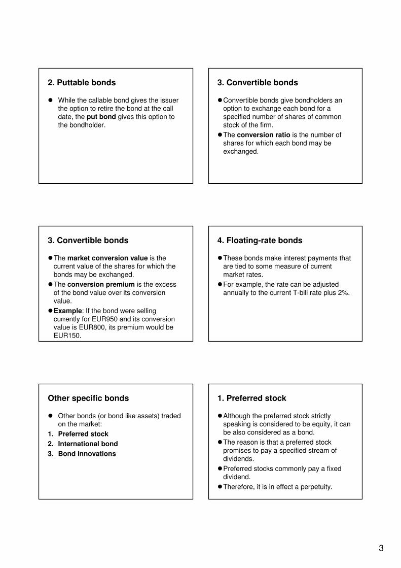
2. Puttable bonds
� While the callable bond gives the issuer the option to retire the bond at the call date, the put bond gives this option to the bondholder.
3. Convertible bonds
�Convertible bonds give bondholders an option to exchange each bond for a specified number of shares of common stock of the firm.
�The conversion ratio is the number of shares for which each bond may be exchanged.
3. Convertible bonds
�The market conversion value is the current value of the shares for which the bonds may be exchanged.
�The conversion premium is the excess of the bond value over its conversion value.
�Example: If the bond were selling currently for EUR950 and its conversion value is EUR800, its premium would be EUR150.
4. Floating-rate bonds
�These bonds make interest payments that are tied to some measure of current market rates.
�For example, the rate can be adjusted annually to the current T-bill rate plus 2%.
Other specific bonds
� Other bonds (or bond like assets) traded on the market:
1. Preferred stock
2. International bond
3. Bond innovations
1. Preferred stock
�Although the preferred stock strictly speaking is considered to be equity, it can be also considered as a bond.
�The reason is that a preferred stock promises to pay a specified stream of dividends.
�Preferred stocks commonly pay a fixed dividend.
�Therefore, it is in effect a perpetuity.
4
1. Preferred stock
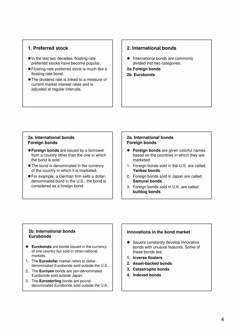
� In the last two decades, floating-rate preferred stocks have become popular.
�Floating-rate preferred stock is much like a floating-rate bond:
�The dividend rate is linked to a measure of current market interest rates and is adjusted at regular intervals.
2. International bonds
� International bonds are commonly divided into two categories:
2a.Foreign bonds
2b. Eurobonds
2a. International bondsForeign bonds
�Foreign bonds are issued by a borrower from a country other than the one in which the bond is sold.
�The bond is denominated in the currency of the country in which it is marketed.
�For example, a German firm sells a dollar-denominated bond in the U.S., the bond is considered as a foreign bond.
2a. International bondsForeign bonds
� Foreign bonds are given colorful names based on the countries in which they are marketed:
1. Foreign bonds sold in the U.S. are called Yankee bonds.
2. Foreign bonds sold in Japan are called Samurai bonds.
3. Foreign bonds sold in U.K. are called bulldog bonds.
2b. International bondsEurobonds
� Eurobonds are bonds issued in the currency of one country but sold in other national markets.
1. The Eurodollar market refers to dollar-denominated Eurobonds sold outside the U.S..
2. The Euroyen bonds are yen-denominated Eurobonds sold outside Japan.
3. The Eurosterling bonds are pound-denominated Eurobonds sold outside the U.K..
Innovations in the bond market
� Issuers constantly develop innovative bonds with unusual features. Some of these bonds are:
1. Inverse floaters
2. Asset-backed bonds
3. Catastrophe bonds
4. Indexed bonds

5
1. Inverse floaters
� These are similar to the floating-rate bonds except that the coupon rate on these bonds falls when the general level of interest rates rises.
� Investors suffer doubly when rates rise:
1. The present value of the future bond payments decreases.
2. The level of the future bond payments decreases.
� Investors benefit doubly when rates fall.
2. Asset-backed bonds
� In asset-backed securities, the income from a specific group of assets is used to service the debt.
�For example, Dawid Bowie bonds have been issued with payments that will be tied to the royalties on some of his albums.
2. Mortgage-backed bonds
�Another example of asset-backed bondsis mortgage-backed security, which is either an ownership claim in a pool of mortgages or an obligation that is secured by such a pool.
�These claims represent securitization of mortgage loans.
�Mortgage lenders originate loans and then sell packages of these loans in the secondary market.
2. Mortgage-backed bonds
�The mortgage originator continues to service the loan, collecting principal and interest payments, and passes these payments to the purchaser of the mortgage.
�For this reason, mortgage-backed securities are called pass-throughs.
3. Catastrophe bonds
�Catastrophe bonds are a way to transfer catastrophe risk from a firm to the market.
�For example, Tokyo Disneyland issued a bond with a final payment that depended on whether there has been an earthquake near the park.
4. Indexed bonds
� Indexed bonds make payments that are tied to a general price index or the price of a particular commodity.
�For example, Mexico issued 20-year bonds with payments that depend on the price of oil.
�The U.S. Treasury issued inflation protected bonds in 1997. (Treasury Inflation Protected Securities, TIPS)
�For TIPS, the coupon and final payment is related to the consumer price index.
6
BOND PRICING
Bond pricing
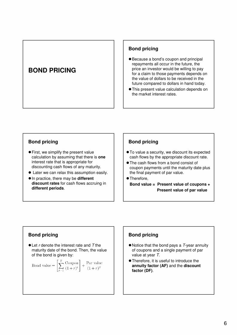
�Because a bond’s coupon and principal repayments all occur in the future, the price an investor would be willing to pay for a claim to those payments depends on the value of dollars to be received in the future compared to dollars in hand today.
�This present value calculation depends on the market interest rates.
Bond pricing
�First, we simplify the present value calculation by assuming that there is oneinterest rate that is appropriate for discounting cash flows of any maturity.
� Later we can relax this assumption easily.
� In practice, there may be different discount rates for cash flows accruing in different periods.
Bond pricing
�To value a security, we discount its expected cash flows by the appropriate discount rate.
�The cash flows from a bond consist of coupon payments until the maturity date plus the final payment of par value.
�Therefore,
Bond value = Present value of coupons +
Present value of par value
Bond pricing
�Let r denote the interest rate and T the maturity date of the bond. Then, the value of the bond is given by:
Bond pricing
�Notice that the bond pays a T-year annuity of coupons and a single payment of par value at year T.
�Therefore, it is useful to introduce the annuity factor (AF) and the discount factor (DF).

7
Annuity factor
�The T-year annuity factor is used to compute the present value of a T-year annuity:
�Notice that AF is a function of the interest rate, r and the time period of the annuity, T.
Discount factor
�The discount factor for period t is used to compute the present value of a cash flow of year t:
�Notice that DF is a function of the interest rate, r and the time of the cash flow payment, t.
Bond pricing
�We can rewrite to previous bond pricing formula using the AF and DF as follows:
Bond pricing
�The bond value has inverse relationshipwith the interest rate used to compute the present value.
�Example: We consider a 30-year bond with par value 100 and coupon rate 8%.
� In the following figure, we present the value of this bond as a function of the interest rate, r.
Bond pricing
Bond value
0.0
50.0
100.0
150.0
200.0
250.0
300.0
350.0
400.0
0.10
%
1.00
%
1.90%
2.80%
3.70
%
4.60%
5.50%
6.40%
7.30
%
8.20
%
9.10%
10.00%
10.90
%
11.8
0%
12.7
0%
13.60%
14.5
0%
15.4
0%
16.3
0%
17.20
%
18.1
0%
19.0
0%
19.9
0%
Interest rate
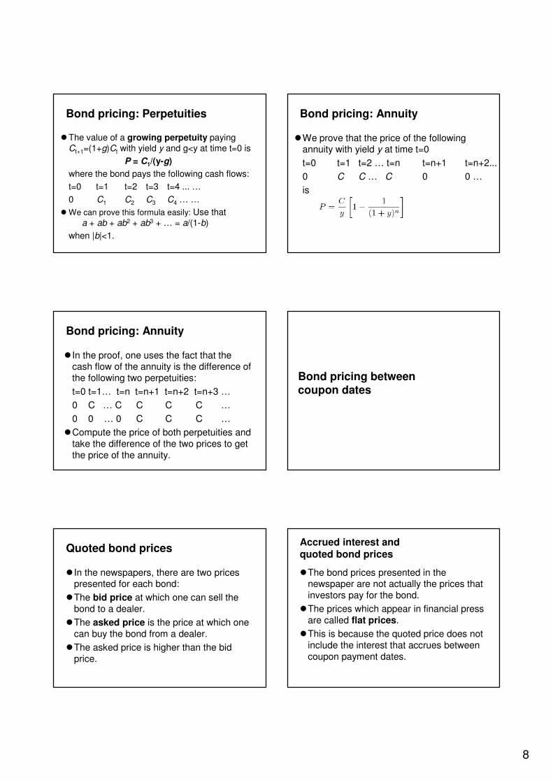
Bond pricing: Perpetuities
�The value of a perpetuity paying Cforever with yield y at time t=0 is
P = C/y
where the bond pays the following cash flows:
t=0 t=1 t=2 t=3 t=4 ...
0 C C C C …
�We can prove this formula easily: Use that a + ab + ab2 + ab3 + … = a/(1-b)
when |b|<1.
8
Bond pricing: Perpetuities
�The value of a growing perpetuity paying Ct+1=(1+g)Ct with yield y and g<y at time t=0 is
P = C1/(y-g)
where the bond pays the following cash flows:
t=0 t=1 t=2 t=3 t=4 ... …
0 C1 C2 C3 C4 … …
� We can prove this formula easily: Use that a + ab + ab2 + ab3 + … = a/(1-b)
when |b|<1.
Bond pricing: Annuity
�We prove that the price of the following annuity with yield y at time t=0
t=0 t=1 t=2 … t=n t=n+1 t=n+2...
0 C C … C 0 0 …
is
Bond pricing: Annuity
� In the proof, one uses the fact that the cash flow of the annuity is the difference of the following two perpetuities:
t=0 t=1… t=n t=n+1 t=n+2 t=n+3 …
0 C … C C C C …
0 0 … 0 C C C …
�Compute the price of both perpetuities and take the difference of the two prices to get the price of the annuity.
Bond pricing between coupon dates
Quoted bond prices
� In the newspapers, there are two prices presented for each bond:
�The bid price at which one can sell the bond to a dealer.
�The asked price is the price at which one can buy the bond from a dealer.
�The asked price is higher than the bid price.
Accrued interest and quoted bond prices
�The bond prices presented in the newspaper are not actually the prices that investors pay for the bond.
�The prices which appear in financial press are called flat prices.
�This is because the quoted price does not include the interest that accrues between coupon payment dates.

9
Accrued interest and quoted bond prices
�The actual invoice price that the buyer pays for the bond includes accrued interest:
Invoice price = Flat price +
Accrued interest
Accrued interest and quoted bond prices
� If a bond is purchased between coupon payments, the buyer must pay the seller for accrued interest, the prorated share of the upcoming semiannual coupon.
Accrued interest and quoted bond prices
�Example: If 30 days have passed since the last coupon payment, and there are 182 days in the semiannual coupon period, the seller is entitled to a payment of accrued interest of 30/182 of the semiannual coupon.
Accrued interest and quoted bond prices
� In general, the formula for the amount of accrued interest between two dates of the semiannual payment is
Accrued interest =
(Annual coupon payment /2) x
(Days since last coupon payment /
Days separating coupon payments)
Bond yields
Yield to maturity
� In practice, an investor considering the purchase of a bond is not quoted a promised rate of return.
� Instead, the investor must use the bond price, maturity date, and coupon payments to infer the return offered by the bond over its life.
�The yield to maturity (YTM) is defined as the interest rate that makes the present value of a bond’s payments equal to its price.

10
Yield to maturity
�The calculate the YTM, we solve the bond price equation for the interest rate given the bond’s price.
�The following YIELD(·) or RENDTO(·) function can be used in English and Spanish language Excel, respectively, to compute the yield to maturity:
YIELD(settlement, maturity, rate, pr, redemption, frequency [,basis])
settlement: The settlement date of the security.maturity: The maturity date of the security.rate: The annual coupon rate of the security.pr: The price per $100 face value.redemption: The security's redemption value per $100
face value.frequency: The number of coupon payments per year:
1 = annual2 = semi-annual4 = quarterly
basis: The type of day counting to use.0 = US 30/3601 = Actual/Actual2 = Actual/3603 = Actual/3654 = European 30/360
Yield to maturity
�YTM differs from the current yield of the bond, which is the bond’s annual coupon payment divided by the bond price.
�For premium bonds (bonds selling above par value), coupon rate is greater than current yield, which is greater than yield to maturity:
YTM < Current yield < Coupon rate
Yield to maturity
�For discount bonds (bonds selling below par value), coupon rate is lower than current yield, which is lower than yield to maturity:
Coupon rate < Current yield < YTM
TERM STRUCTURE OF
INTEREST RATES
TERM STRUCTURE OF INTEREST RATES
�The term structure of interest rates is represented by the yield curve.
�The yield curve is a plot of yield to maturity (YTM) as a function of time to maturity.
� If yields on different-maturity bonds are not equal, how should we value coupon bonds that make payments at many different times?

11
TERM STRUCTURE OF INTEREST RATES
�Example: Suppose that zero-coupon bonds with 1-year maturity sell at YTM y1=5%, 2-year zeros sell at YTM y2=6% and 3-year zeros sell at YTM y3=7%.
�Which of these rates should we use to discount bond cash flows?
�ALL OF THEM.
�The trick is to consider each bond cash flow – either coupon or par value payment – as a zero-coupon bond.
TERM STRUCTURE OF INTEREST RATES
�Example (continued): Price a bond paying the following cash flow:
t=1 100
t=2 100
t=3 1100
1082.2Bond value:
897.90.8167%11003
89.00.8906%1002
95.20.9525%1001
Present valueDF(r,t)RateCash flowPeriod
TERM STRUCTURE OF INTEREST RATES
�Example (continued):
In the previous table, bond value is computed by the following formulas:
ZERO-COUPON BONDS
� In the previous example, we used the yields of the zero-coupon bonds to discount future cash flows.
�Zero-coupon bonds are maybe the most important bonds because they can be used to build up other bonds with more complicated cash flow structure.
�When the prices of zero-coupon bonds are known, they can be used to price more complicated bonds.
SPOT RATE
�Practitioners call the yield to maturity on zero-coupon bonds spot rate meaning the rate that prevails today for a time period corresponding to the zero’s maturity.
�We denote the spot rates for the time periods t =1,2,…,T as follows:
{y1,y2,…,yT}
�The sequence of the spot rates over t=1,..,T defines the SPOT YIELD CURVE:
{y1,y2,…,yT}
SHORT RATE
� In contrast, the short rate for a given time interval (for example 1 year) refers to the interest rate for that interval available at different points of time of the future.
�We denote the 1-year short rate for the time period t as:
t-1rt
More generally, for time periods 1 ≤ t ≤ T:
{0r1,1r2,2r3,….,T-1rT}

12
SHORT RATE AND SPOT RATE
� We shall relate the spot and short rates in two alternative situations:
1. Future interest rates are certain.
2. Future interest rates are uncertain.
SHORT AND SPOT RATES:FUTURE RATES ARE CERTAIN
�The spot rates can be computed knowing the short rates because:
(1+yt)t = (1+0r1)(1+1r2)…(1+t-1rt)
�Notice that y1 = 0r1.
�The short rates can be computed knowing the spot rates because:
t-1rt = [(1+yt)t/(1+yt-1)
t-1] - 1
�THE ASSUMPTION IN THESE FORMULAS IS THAT FUTURE SHORT RATES ARE KNOWN WITH CERTAINTY.
SHORT AND SPOT RATES
�Example: Consider two alternative investment strategies for investing 1 euro during 2 periods:
t=0 t=1 t=2
t=0 t=1 t=2
1
1
(1+y2)2
(1+y1)(1+1r2)1+y1
SHORT AND SPOT RATES:FUTURE RATES ARE UNCERTAIN
�However, in the reality, future short rates are not known.
�Nevertheless, it is still common to investigate the implications of the yield curve for future interest rates.
FORWARD INTEREST RATE
�Recognizing that future interest rates are uncertain, we call the interest rate that we infer in this manner the forward interest rate or the future short rate, denoted t-1ftfor period t, because it need not be the interest rate that actually will prevail at the future date.
�The sequence of forward rates for periods t=1,…,T defines the FORWARD YIELD CURVE: {1f2,2f3,…,T-1fT}
FORWARD INTEREST RATE
� If the 1-year forward rate for period t is denoted t-1ft we then define t-1ft by the next equation:
t-1ft = [(1+yt)t/(1+yt-1)
t-1] - 1
�Equivalently, we can express the spot rate for period t using the forward rates as follows:
(1+yt)t = (1+0f1)(1+1f2)…(1+t-1ft)
�Notice that 0f1 = y1.

13
SHORT AND FORWARD INTEREST RATES
�We emphasize that the interest rate that actually will prevail in the future need not equal the forward rate, which is calculated from today’s data.
� Indeed, it is not even necessary the case that the forward rate equals the expected value of the future short rate.
SHORT AND FORWARD INTEREST RATES
�The difference between the forward rate and the future short rate is called liquidity premium.
�The name comes from the fact that the forward rate determines the interest that long-term investors obtain while short-term investors are more interested in the future short-rate.
SHORT AND FORWARD INTEREST RATES
� In order to relate the future short rates with forward rates, economists worked out several alternative theories.
� These are called theories of term structure. We will see two alternative theories:
1. Expectation hypothesis
2. Liquidity preference theory
EXPECTATION HYPOTHESIS
�The expectation hypothesis is the simplest theory of term structure.
� It states that the forward rate equals the market consensus expectation of the future short interest rate for all periods t:
t-1ft = E[t-1rt]
LIQUIDITY PREFERENCE
� In this theory, we have two types of investors:
1. Short-term investors: They prefer to invest for short time horizons.
2. Long-term investors: They prefer to invest for long time horizons.
LIQUIDITY PREFERENCE
�Short-term investors are willing to hold long-term bonds if
t-1ft > E[t-1rt]
�Long-term investors are willing to hold short-term bonds if
t-1ft < E[t-1rt]

14
LIQUIDITY PREFERENCE
�People who believe in the liquidity preference theory think that short-term investors dominate the market.
�Therefore, in general the forward rate is higher than the future short rate:
t-1ft > E[t-1rt]
�Therefore, the liquidity premium is positive:
Liquidity premium = t-1ft - E[t-1rt] > 0
LIQUIDITY PREFERENCE
� In the liquidity preference theory,
Forward rate = Short rate + Liquidity premium
� Therefore, the shape of the forward yield curve is determined by two components:
1. Investors’ expectations about future interest rates (short rate component) and
2. Investors’ future liquidity premium requirements (liquidity premium component).
FORWARD RATES AS FORWARD CONTRACTS
�We have seen how the forward rates can be derived from the spot yield curve.
�Why are these forward rates important from practical point of view?
�There is an important sense in which the forward rate is a market interest rate:
FORWARD RATES AS FORWARD CONTRACTS
�Suppose that you wanted to arrange nowto make a loan at some future date.
�You would agree today on the interest rate that will be charged, but the loan would not commence until some time in the future.
�How would the interest rate on such a “forward loan” be determined?
�We will show that the interest rate of this forward loan would be the forward rate.
FORWARD RATES AS FORWARD CONTRACTS
Example:
�Suppose the price of 1-year maturity zero-coupon bond with face value EUR1000 is EUR952.38 and
� the price of 2-year zero-coupon bond with face value EUR1000 is EUR890.
FORWARD RATES AS FORWARD CONTRACTS
�We can determine two spot rates and the forward rate for the second period:
y1 = 1000 / 952.38 – 1 = 5%
y2 = (1000 / 890)1/2 – 1 = 6%
1f2 = (1+y2)2 / (1+y1) – 1 = 7.01%

15
FORWARD RATES AS FORWARD CONTRACTS
� Now consider the following strategy:
1. Buy one unit 1-year zero-coupon bond
2. Sell 1.0701 unit 2-year zero-coupon bonds
� In the followings, we review the cash flows of this strategy:
FORWARD RATES AS FORWARD CONTRACTS
� At t=0, initial cash flow:
1. Long one one-year zero:
-952.38 EUR
2. Short 1.0701 two-year zeros:
+890 x 1.0701 = 952.38 EUR
TOTAL cash flow at t=0:
- 952.38 + 952.38 = 0
FORWARD RATES AS FORWARD CONTRACTS
� At t=1, cash flow:
1. Long one one-year zero:
+1000 EUR
2. Short 1.0701 two-year zero:
0 EUR
TOTAL cash flow at t=1:
+1000 EUR
FORWARD RATES AS FORWARD CONTRACTS
� At t=2, cash flow:
1. Long one one-year zero:
0 EUR
2. Short 1.0701 two-year zero:
-1.0701 x 1000 EUR = - 1070.01 EUR
TOTAL cash flow at t=2:
-1070.01 EUR
FORWARD RATES AS FORWARD CONTRACTS
� In summary, we present the total cash flows over the two periods:
t=0 t=1 t=2
0 EUR +1000 EUR -1070.01 EUR
�Thus, we can see that the strategy creates a synthetic “forward loan”: borrowing 1000 at t=1 and paying 1070.01 at t=2.
�Notice that the interest rate of this loan is
1070.01/1000 – 1 = 7.01%
which is equal to the forward rate.
FORWARD RATES AS FORWARD CONTRACTS
�Therefore, we can synthetically construct a forward loan by buying a shorter maturity zero-coupon bond and short selling a longer maturity zero-coupon bond.
�The interest rate of this forward loan is determined by the forward rate.
16
YIELD CURVE ESTIMATION
ESTIMATING THE YIELD CURVE
� We talked about how can we use the values of the spot yield curve in order to discount future cash flows.
� However, in the reality we do not observe the yield curve.
� In the real world, we observe:
1. The bid and asked prices of bonds
2. The cash flows of coupon and par value payments of bonds.
ESTIMATING THE YIELD CURVE
� It is useful from a practical point of view to estimate the spot yield curve because it helps us to discount cash flows paid at any time in the future.
�Therefore, given the yield curve we can price any fixed-income financial asset on the market.
ESTIMATING THE YIELD CURVE
� In this section, we review a methodology to estimate the spot yield curve given the observed bond prices and future cash flow payments.
ESTIMATING THE YIELD CURVE
�We will start with observed data on (1) bid and asked prices, (2) accrued interest and (3) future cash flows of several bonds traded on the market.
�We also know the exact day of each cash flow payment.
� In order to estimate the spot yield curve, we proceed as follows:
ESTIMATING THE YIELD CURVE
1. Compute the market price, p for each bond by the next formula:
p = (Asked price + Bid price)/2
+ Accrued interest
17
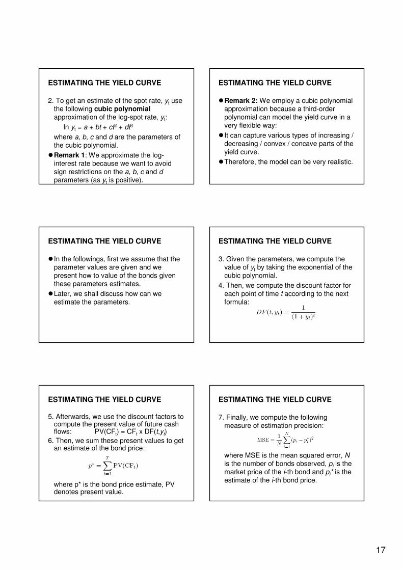
ESTIMATING THE YIELD CURVE
2. To get an estimate of the spot rate, yt use the following cubic polynomialapproximation of the log-spot rate, yt:
ln yt = a + bt + ct2 + dt3
where a, b, c and d are the parameters of the cubic polynomial.
�Remark 1: We approximate the log-interest rate because we want to avoid sign restrictions on the a, b, c and dparameters (as yt is positive).
ESTIMATING THE YIELD CURVE
�Remark 2: We employ a cubic polynomial approximation because a third-order polynomial can model the yield curve in a very flexible way:
� It can capture various types of increasing / decreasing / convex / concave parts of the yield curve.
�Therefore, the model can be very realistic.
ESTIMATING THE YIELD CURVE
� In the followings, first we assume that the parameter values are given and we present how to value of the bonds given these parameters estimates.
�Later, we shall discuss how can we estimate the parameters.
ESTIMATING THE YIELD CURVE
3. Given the parameters, we compute the value of yt by taking the exponential of the cubic polynomial.
4. Then, we compute the discount factor for each point of time t according to the next formula:
ESTIMATING THE YIELD CURVE
5. Afterwards, we use the discount factors to compute the present value of future cash flows: PV(CFt) = CFt x DF(t,yt)
6. Then, we sum these present values to get an estimate of the bond price:
where p* is the bond price estimate, PV denotes present value.
ESTIMATING THE YIELD CURVE
7. Finally, we compute the following measure of estimation precision:
where MSE is the mean squared error, Nis the number of bonds observed, pi is the market price of the i-th bond and pi* is the estimate of the i-th bond price.

18
ESTIMATING THE YIELD CURVE
�How do we choose the values of the parameters?
�We choose parameter values such that the MSE precision measure is minimized.
�The MSE minimization can be done numerically in Excel using the SOLVERtool.
� (In Excel use: Tools / Solver or Herramientas / Solver.)
ESTIMATING THE YIELD CURVE
�The following figure show the spot yield curve estimate for Hungarian government bond data for the 1997-2002 period:
ESTIMATING THE YIELD CURVE
SPOT YIELD CURVE, y(t)
0.00%
5.00%
10.00%
15.00%
20.00%
25.00%
9/21
/199
7
1/21
/199
8
5/21
/199
8
9/21
/199
8
1/21
/199
9
5/21
/199
9
9/21
/199
9
1/21
/200
0
5/21
/200
0
9/21
/200
0
1/21
/200
1
5/21
/200
1
9/21
/200
1
1/21
/200
2
5/21
/200
2
Date
MANAGING BOND
PORTFOLIOS
MANAGING BOND PORTFOLIOS
� We are going to review several topics related to bond portfolio management.
� In particular, we shall see:
1. Evolution of bond prices over time
2. Interest rate risk of bonds
3. Default or credit risk of bonds
EVOLUTION OF
BOND PRICES OVER TIME

19
EVOLUTION OF BOND PRICES OVER TIME
� In this section we are going to be in a dynamic framework.
� That is we shall analyze the evolution of the bond price over several periods:
� t=0,1,2,…,T.
EVOLUTION OF BOND PRICES OVER TIME
�As we have discussed before, the determinants of bond value are:
1.Future cash flow payments (i.e., coupon payments and par value payments)
2. Values of the yield-to-maturity (YTM) or spot yield curve used to discount these cash flows.
EVOLUTION OF BOND PRICES OVER TIME
� Future cash flows are fixed in the contract, therefore, they are time invariant. (Supposing that there is no default! In this section, we assume that there is no default risk. We shall see default risk later.)
� However, the YTM or the yield curve may change over time.
EVOLUTION OF BOND PRICES OVER TIME
�We shall investigate the evolution of bond price under two alternative situations:
1.The YTM and spot yield curve are constant over time (NOT REALISTIC ASSUMPTION but it helps to understand a basic characteristic of the bond price evolution.)
2.The YTM and spot yield curve are changeover time (MORE REALISTIC SETUP)
1. YTM and spot yield curve are constant
�When the market price of a bond is observed over several periods t = 1,…,T, we find that the price of the bond is converging to its par value.
�When we have a premium bond then the price of the bond is higher than the par value.
�Therefore, the bond price is decreasing during its convergence.
1. YTM and spot yield curve are constant
�On the other hand, when we have a discount bond then the price of the bond is lower than the par value.
�Therefore, the bond price is increasing during its convergence.
�The convergence of the bond price to its par value, under constant YTM, can be observed on the following figure:

20
1. YTM and spot yield curve are constant
880
900
920
940
960
980
1,000
1,020
1,040
1,060
1,080
0 5 10 15 20 25 30
Time to Maturity
Bo
nd
Pri
ce
Price path for
Premium Bond
Price path for Discount
BondTodayMaturity
2. YTM and spot yield curve are changing
� In the reality, the level of the yield (YTM and spot yield curve) that is used to discount future cash flows is not constant.
�As the relation between the changing YTM and the fixed coupon rate may change, bonds may be discount or premium bonds over time.
2. YTM and spot yield curve are changing
�The following figure presents the evolution of bond price over time when YTM is changing over time:
2. YTM and spot yield curve are changing
Bond value convergence to par value with
changing interest rate
0.0
100.0
200.0
300.0
400.0
500.0
600.0
700.0
800.0
900.0
1000.0
1 13 25 37 49 61 73 85 97 109 121 133 145 157 169 181 193 205 217 229 241 253 265 277 289
period
Bond value
Par value
2. YTM and spot yield curve are changing
�We obtained different yield for each period by Monte Carlo simulation from the following AR(1) process of log-return:
ln rt = c + φ ln rt-1 + ψ ut
where c, φ and ψ are parameters and ut ~ N(0,1) i.i.d is the error term.
�After simulating ln rt we take the exponential of it to get rt.
�Note: We model log-return to ensure to the positivity of yield.
2. YTM and spot yield curve are changing
�As the yield is not constant, in some periods the bond value is higher than the par value and in other periods it is lower than the par value.
�However, in the figure we can see the convergence of the bond price to the par value as we approach to maturity.
� In the Excel spreadsheet, you can re-simulate the yield process with alternative parameters using the “F9” button.

21
INTEREST RATE RISK
INTEREST RATE RISK
�From the previous figure we can see that although bonds promise a fixed income payment over time, the actual price of a bond is affected by the level of interest rates.
�Therefore, fixed income securities are not risk-free.
�Before the time of maturity, their prices are volatile as they are impacted by the changing interest rate.
INTEREST RATE RISK
�The sensitivity of bond price to the interest rate is called interest rate risk.
� Interest rate risk we only have before maturity because the bond promises a fixed par value payment at maturity.
�The only case when the evolution of interest rates is important for the investor is when the investor wants to sell the bond before its maturity time.
INTEREST RATE RISK
� If an investor wants to avoid interest rate risk then it is enough to purchase a bond that will be held until the maturity time of the bond.
�By doing this, it is not important for the investor how the rates change during the lifetime of the bond.
�At maturity time, the investor will receive the fixed par value.
MANAGING INTEREST RATE RISK
�When an investor is interested in bond prices before the maturity time of bond then he is interested in the management of interest rate risk of his bond portfolio.
�A central concept of interest rate risk management is the duration and the modified duration of the bond portfolio.
DURATION
�The duration is the weighted average of the times of each coupon payment where the weights, wt are
where y is the YTM of the bond and duration is computed as

22
DURATION
� The duration can be interpreted as the effective average maturity of the bond portfolio.
� The scale of the duration is years.
Remarks about DURATION
(1) The duration of a zero-coupon bond is equal to the maturity of the zero-coupon bond: D=T.
(2) The duration of a T-period annuity is:
D=(1+y)/y – T / [(1+y)T – 1]
(3) The duration of a perpetuity is
D=(1+y)/y
where y is the yield of the annuity and perpetuity in (2) and (3).
MODIFIED DURATION
�The modified duration for any bond is defined as
where y is the YTM of the bond.
MODIFIED DURATION
• Modified duration can be used to compute the interest rate sensitivity of bond prices because:
where P is the bond price, y is the YTM
MODIFIED DURATION
�The modified duration also helps to answer the following more practical question:
�Question: What is the percentage change of the pond price when the interest rate changes by ∆y?
�Answer: When the interest rate change is relatively small than the percentage price change is approximately:
MODIFIED DURATION
�Remark: Notice that if the duration (or modified duration) of a bond is higher then its interest rate sensitivity will be higher.
� In other words, bonds with longer maturity time are more sensitive to changes of the interest rate.
� In other words, interest rate risk of long maturity bonds is higher than that of short maturity bonds.
23
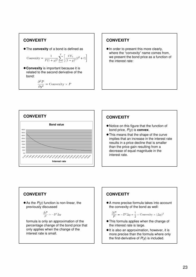
CONVEXITY
�The convexity of a bond is defined as
�Convexity is important because it is related to the second derivative of the bond:
CONVEXITY
� In order to present this more clearly, where the “convexity” name comes from, we present the bond price as a function of the interest rate:
CONVEXITY
Bond value
0.0
50.0
100.0
150.0
200.0
250.0
300.0
350.0
400.0
0.10%
1.00
%
1.90
%
2.80%
3.70
%
4.60
%
5.50%
6.40%
7.30
%
8.20
%
9.10%
10.00%
10.90
%
11.8
0%
12.7
0%
13.60%
14.5
0%
15.4
0%
16.30%
17.20
%
18.1
0%
19.0
0%
19.90%
Interest rate
CONVEXITY
�Notice on this figure that the function of bond price, P(y) is convex.
�This means that the shape of the curve implies that an increase in the interest rate results in a price decline that is smaller than the price gain resulting from a decrease of equal magnitude in the interest rate.
CONVEXITY
�As the P(y) function is non-linear, the previously discussed
formula is only an approximation of the percentage change of the bond price that only applies when the change of the interest rate is small.
CONVEXITY
�A more precise formula takes into account the convexity of the bond as well:
�This formula applies when the change of the interest rate is large.
� It is also an approximation, however, it is more precise than the formula where only the first-derivative of P(y) is included.
24
IMMUNIZATION
�Some financial institutions like banks or pension funds have fixed-income financial products in both the assets and liabilities sides of their balances.
IMMUNIZATION
�Example: A pension fund is receiving fixed payments from young clients who are working and paying every month the pension fund to get pension after their retirement. These payments are in the asset side of the balance.
� In the same time, the pension fund pays fixed monthly pensions to retired pensioners. These payments are on the liability side of the balance.
IMMUNIZATION
�These payments can be seen as bond portfolios.
�Therefore, they are subject to interest rate risk.
�How can a financial company manage the interest rate risk of its assets and liabilities?
�By doing IMMUNIZATION.
IMMUNIZATION
� Immunization means that the duration of assets and liabilities of the company are equal:
DA = DL
�When assets and liabilities of financial firms are immunized then a rate change has the same impact on its assets and liabilities.
�This where the name “immunization”comes from.
DEFAULT OF BONDS: CREDIT RISK
Default risk
�Although bonds generally promise a fixed flow of income, that income stream is not risk-free unless the issuer will not defaulton the obligation.
�While most government bonds may be treated as assets free of default risk, this is not true for corporate bonds.
25
Default risk
� Bond default risk, usually called credit risk, is measured by the next firms:
1. Moody’s,
2. Standard and Poor’s (S&P’s) and
3. Fitch
These institutions provide financial information on firms as well as quality ratings of large corporate and municipal bond issues.
Default risk
� International bonds, especially in emerging markets, also are commonly rated for default risk.
�Each rating firm assigns letter grades to the bonds to reflect their assessment of the safety of the bond issue.
� In the following table, the grades of Moody’s and Standard and Poor’s are presented:
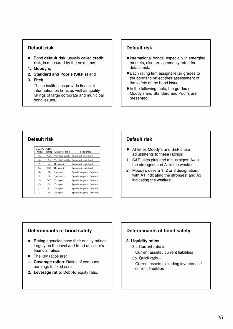
Default risk
Speculative-grade / Junk bondVery poorDD
Speculative-grade / Junk bondVery poorCC
Speculative-grade / Junk bondVery poorCCCa
Speculative-grade / Junk bondVery poorCCCCaa
Speculative-grade / Junk bondSpeculativeBB
Speculative-grade / Junk bondSpeculativeBBBa
Investment-grade bondHigh qualityBBBBaa
Investment-grade bondHigh qualityAA
Investment-grade bondVery high qualityAAAa
Investment-grade bondVery high qualityAAAAaa
Bond gradeQuality of bond
S&P's
rating
Moody's
rating
Default risk
� At times Moody’s and S&P’s use adjustments to these ratings:
1. S&P uses plus and minus signs: A+ is the strongest and A- is the weakest.
2. Moody’s uses a 1, 2 or 3 designation, with A1 indicating the strongest and A3 indicating the weakest.
Determinants of bond safety
� Rating agencies base their quality ratings largely on the level and trend of issuer’s financial ratios.
� The key ratios are:
1. Coverage ratios: Ratios of company earnings to fixed costs.
2. Leverage ratio: Debt-to-equity ratio.
Determinants of bond safety
3. Liquidity ratios:
3a. Current ratio =
Current assets / current liabilities
3b. Quick ratio =
Current assets excluding inventories / current liabilities
26
Determinants of bond safety
4. Profitability ratios: Measures of rates of return on assets or equity
4a. Return on assets (ROA) =
Net income / total assets
4b. Return on equity (ROE) =
Net income / equity
5. Cash flow-to-debt ratio: Ratio of total cash flow to outstanding debt
Default premium
�To compensate for the possibility of default, corporate bonds must offer a default premium.
�The default premium is the difference between the promised yield on a corporate bond and the yield of an otherwise identical government bond that is risk-free in terms of default.
Default premium
� If the firm remains solvent and actually pays the investor all of the promised cash flows, the investor will realize a higher yield to maturity than would be realized from the government bond.
�However, if the firm goes bankrupt, the corporate bond will likely to provide a lower return than the government bond.
�That is why the corporate bond is riskier than the government bond.
Default premium
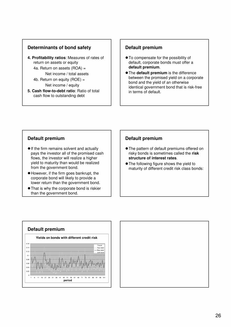
�The pattern of default premiums offered on risky bonds is sometimes called the risk structure of interest rates.
�The following figure shows the yield to maturity of different credit risk class bonds:
Default premium
Yields on bonds with different credit risk
0
0.02
0.04
0.06
0.08
0.1
0.12
0.14
0.16
1 6 11 16 21 26 31 36 41 46 51 56 61 66 71 76 81 86 91 96 101
period
T-bond
Aaa rated
Baa rated
Junk bond
27
DERIVATIVES
DERIVATIVES
A derivative is a financial instrument that is derived from some other asset (known as the underlying asset).
Rather than trade or exchange the underlying asset itself, derivative traders enter into an agreement that involves a final payoff which depends on the price of the underlying asset.
A GENERAL DEFINITION OF DERIVATIVES
�The final payoff of a derivative is always a specific function of past and current prices of the underlying asset.
(Payoff of derivative at time t) = f (S1,…,St)
where St is the price of the underlying asset at time t and f (·) is the payoff function of the derivative.
A GENERAL DEFINITION OF RELATIVELY SIMPLE DERIVATIVES
�The payoff of the more simple derivatives depends only on the current price of the underlying asset:
(Payoff of derivative at time t) = f (St)
�Most derivatives that we see in this course have this type of payoff function.
A REMARK
�The word “derivative” has nothing to do with the derivative that you have studied in differentiation during the mathematical calculus course.
�The word “derivative” refers to the fact that the payoff of a derivative is a function of the price of the underlying asset.
�The payoff function defines the derivative.
�Different derivatives have different payoff functions.
DERIVATIVES
� Important types of derivatives are:
1. FUTURES and FORWARDS
2. OPTIONS
3. SWAPS

28
FUTURES
FUTURES
� A contract to buy or sell an asset on a future date at a fixed price.
� The buyer and the seller of the futures contract have the obligation to buy or sell the asset.
FUTURES
�The buyer of the futures contract is in long futures position.
�The seller of the futures contract is in short futures position.
FUTURES
�The underlying asset of the futures contract can be:
1. Commodity like grain, metals or energy
2. Financial product like interest rate, exchange rate, stock or stock index
ELEMENTS OF FUTURES CONTRACT
� The main elements of the futures contract are the
1. Futures price, F
This is the price fixed in the contract at which the transaction will occur in the future.
2. Expiration date, T
This is the date fixed in the contract when the delivery will take place in the future.
PAYOFF OF FUTURES CONTRACT
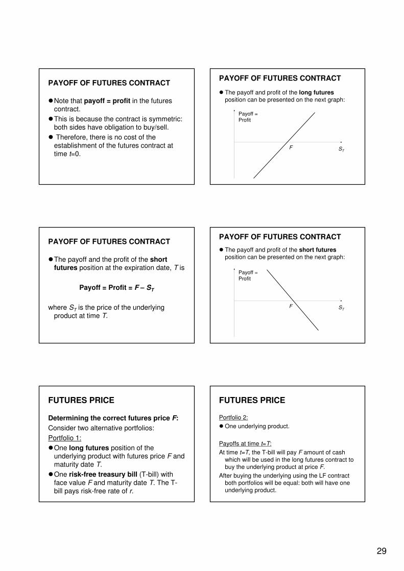
�The payoff and the profit of the long futures position at the expiration date, T is
Payoff = Profit = ST – F
where ST is the price of the underlying product at time T.
29
PAYOFF OF FUTURES CONTRACT
�Note that payoff = profit in the futures contract.
�This is because the contract is symmetric: both sides have obligation to buy/sell.
� Therefore, there is no cost of the establishment of the futures contract at time t=0.
PAYOFF OF FUTURES CONTRACT
� The payoff and profit of the long futuresposition can be presented on the next graph:
F ST
Payoff = Profit
PAYOFF OF FUTURES CONTRACT
�The payoff and the profit of the short futures position at the expiration date, T is
Payoff = Profit = F – ST
where ST is the price of the underlying product at time T.
PAYOFF OF FUTURES CONTRACT
� The payoff and profit of the short futuresposition can be presented on the next graph:
Payoff = Profit
STF
FUTURES PRICE
Determining the correct futures price F:
Consider two alternative portfolios:
Portfolio 1:
�One long futures position of the underlying product with futures price F and maturity date T.
�One risk-free treasury bill (T-bill) with face value F and maturity date T. The T-bill pays risk-free rate of r.
FUTURES PRICE
Portfolio 2:
� One underlying product.
Payoffs at time t=T:
At time t=T, the T-bill will pay F amount of cash which will be used in the long futures contract to buy the underlying product at price F.
After buying the underlying using the LF contract both portfolios will be equal: both will have one underlying product.
30
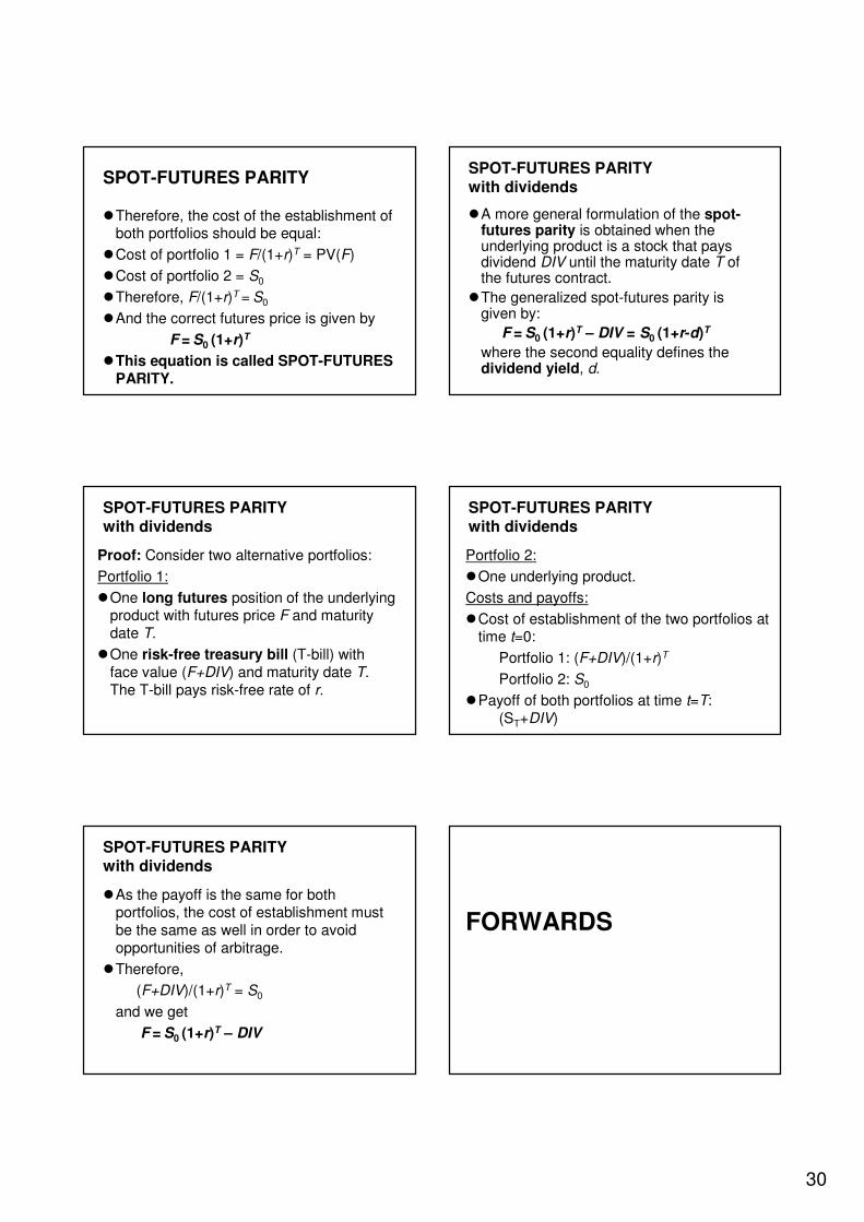
SPOT-FUTURES PARITY
�Therefore, the cost of the establishment of both portfolios should be equal:
�Cost of portfolio 1 = F/(1+r)T = PV(F)
�Cost of portfolio 2 = S0
�Therefore, F/(1+r)T = S0
�And the correct futures price is given by
F = S0 (1+r)T
�This equation is called SPOT-FUTURES PARITY.
SPOT-FUTURES PARITY with dividends
�A more general formulation of the spot-futures parity is obtained when the underlying product is a stock that pays dividend DIV until the maturity date T of the futures contract.
�The generalized spot-futures parity is given by:
F = S0 (1+r)T – DIV = S0 (1+r-d)T
where the second equality defines the dividend yield, d.
SPOT-FUTURES PARITY with dividends
Proof: Consider two alternative portfolios:
Portfolio 1:
�One long futures position of the underlying product with futures price F and maturity date T.
�One risk-free treasury bill (T-bill) with face value (F+DIV) and maturity date T. The T-bill pays risk-free rate of r.
SPOT-FUTURES PARITY with dividends
Portfolio 2:
�One underlying product.
Costs and payoffs:
�Cost of establishment of the two portfolios at time t=0:
Portfolio 1: (F+DIV)/(1+r)T
Portfolio 2: S0
�Payoff of both portfolios at time t=T: (ST+DIV)
SPOT-FUTURES PARITY with dividends
�As the payoff is the same for both portfolios, the cost of establishment must be the same as well in order to avoid opportunities of arbitrage.
�Therefore,
(F+DIV)/(1+r)T = S0
and we get
F = S0 (1+r)T – DIV
FORWARDS
31
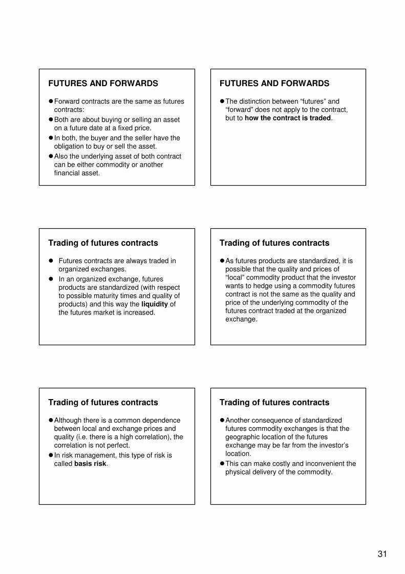
FUTURES AND FORWARDS
�Forward contracts are the same as futures contracts:
�Both are about buying or selling an asset on a future date at a fixed price.
� In both, the buyer and the seller have the obligation to buy or sell the asset.
�Also the underlying asset of both contract can be either commodity or another financial asset.
FUTURES AND FORWARDS
�The distinction between “futures” and “forward” does not apply to the contract, but to how the contract is traded.
Trading of futures contracts
� Futures contracts are always traded in organized exchanges.
� In an organized exchange, futures products are standardized (with respect to possible maturity times and quality of products) and this way the liquidity of the futures market is increased.
Trading of futures contracts
�As futures products are standardized, it is possible that the quality and prices of “local” commodity product that the investor wants to hedge using a commodity futures contract is not the same as the quality and price of the underlying commodity of the futures contract traded at the organized exchange.
Trading of futures contracts
�Although there is a common dependence between local and exchange prices and quality (i.e. there is a high correlation), the correlation is not perfect.
� In risk management, this type of risk is called basis risk.
Trading of futures contracts
�Another consequence of standardized futures commodity exchanges is that the geographic location of the futures exchange may be far from the investor’s location.
�This can make costly and inconvenient the physical delivery of the commodity.

32
Trading of futures contracts
�Because of this reason, frequently, futures contracts are closed just before the maturity date and the corresponding profit or loss is delivered in cash.
�Closing a futures position means to open an opposite futures position to cancel the payoffs of both positions.
�For example, an investor having a LF position can close this by opening a SF position.
Trading of futures contracts
�When a futures contract is bought or sold, the investor is asked to put up a margin in the form of either cash or Treasury-bills to demonstrate that he has the money to finance his side of the bargain.
� In addition, futures contracts are marked-to-market. This means that each day any profit or losses on the contract are calculated and the investor pays the exchange any losses and receive any profits.
Trading of futures contracts
� For example, famous futures exchanges in the U.S. are:
1. Chicago Mercantile Exchange Group (CME Group) that was formed by the fusion of Chicago Board of Trade (CBOT) and Chicago Mercantile Exchange (CME).
2. New York Mercantile Exchange (NYMEX).
Trading of forward contracts
�Liquidity of futures exchanges is high because of standardization of the futures contracts.
�However, if the terms of the futures contracts do not suit the particular needs of the investor, he may able to buy or sell forward contracts.
Trading of forward contracts
� The main forward market is in foreign currency. (Forex market or FX market)
� It is also possible to enter into a forward interest rate contract called forward rate agreement (FRA).
OPTIONS
33
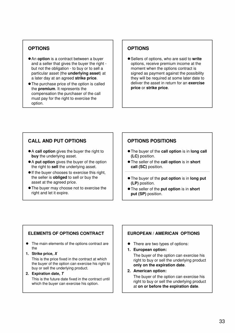
OPTIONS
�An option is a contract between a buyer and a seller that gives the buyer the right -but not the obligation - to buy or to sell a particular asset (the underlying asset) at a later day at an agreed strike price.
�The purchase price of the option is called the premium. It represents the compensation the purchaser of the call must pay for the right to exercise the option.
OPTIONS
�Sellers of options, who are said to writeoptions, receive premium income at the moment when the options contract is signed as payment against the possibility they will be required at some later date to deliver the asset in return for an exercise price or strike price.
CALL AND PUT OPTIONS
�A call option gives the buyer the right to buy the underlying asset.
�A put option gives the buyer of the option the right to sell the underlying asset.
� If the buyer chooses to exercise this right, the seller is obliged to sell or buy the asset at the agreed price.
�The buyer may choose not to exercise the right and let it expire.
OPTIONS POSITIONS
�The buyer of the call option is in long call (LC) position.
�The seller of the call option is in short call (SC) position.
�The buyer of the put option is in long put (LP) position.
�The seller of the put option is in short put (SP) position.
ELEMENTS OF OPTIONS CONTRACT
� The main elements of the options contract are the
1. Strike price, X
This is the price fixed in the contract at which the buyer of the option can exercise his right to buy or sell the underlying product.
2. Expiration date, T
This is the future date fixed in the contract until which the buyer can exercise his option.
EUROPEAN / AMERICAN OPTIONS
� There are two types of options:
1. European option:
The buyer of the option can exercise his right to buy or sell the underlying product only on the expiration date.
2. American option:
The buyer of the option can exercise his right to buy or sell the underlying product at on or before the expiration date.

34
PAYOFF OF OPTIONS
� In the following slides, we show the payoff and the profit of the call and put options.
� We shall use the following notation:
1. X: strike price
2. T: expiration date
3. ST: price of underlying product on the expiration date
4. c: premium of the call option
5. p: premium of the put option
PAYOFF OF LONG CALL
�The payoff of the European long call position is
Payoff LC = max {ST – X,0}
Payoff
STX
PROFIT OF LONG CALL
�The profit of the European long call position is
Profit LC = max {ST – X,0} – c
Profit
X
STc
PAYOFF OF SHORT CALL
�The payoff of the European short call position is
Payoff SC = - max {ST – X,0}
Payoff
ST
X
PROFIT OF SHORT CALL
�The profit of the European short call position is
Profit SC = - max {ST – X,0} + c
STX
Profit
c
PAYOFF OF LONG PUT
�The payoff of the European long put position is
Payoff LP = max {X – ST,0}
Payoff
STX
35
PROFIT OF LONG PUT
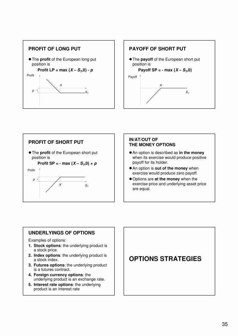
�The profit of the European long put position is
Profit LP = max {X – ST,0} - p
X
ST
Profit
p
PAYOFF OF SHORT PUT
�The payoff of the European short put position is
Payoff SP = - max {X – ST,0}
Payoff
ST
X
PROFIT OF SHORT PUT
�The profit of the European short put position is
Profit SP = - max {X – ST,0} + p
X ST
Profit
p
IN/AT/OUT OF THE MONEY OPTIONS
�An option is described as in the moneywhen its exercise would produce positive payoff for its holder.
�An option is out of the money when exercise would produce zero payoff.
�Options are at the money when the exercise price and underlying asset price are equal.
UNDERLYINGS OF OPTIONS
Examples of options:
1. Stock options: the underlying product is a stock price.
2. Index options: the underlying product is a stock index.
3. Futures options: the underlying product is a futures contract.
4. Foreign currency options: the underlying product is an exchange rate.
5. Interest rate options: the underlying product is an interest rate
OPTIONS STRATEGIES
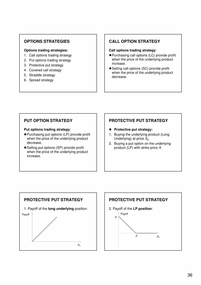
36
OPTIONS STRATEGIES
Options trading strategies:
1. Call options trading strategy
2. Put options trading strategy
3. Protective put strategy
4. Covered call strategy
5. Straddle strategy
6. Spread strategy
CALL OPTION STRATEGY
Call options trading strategy:
�Purchasing call options (LC) provide profit when the price of the underlying product increase.
�Selling call options (SC) provide profit when the price of the underlying product decrease.
PUT OPTION STRATEGY
Put options trading strategy:
�Purchasing put options (LP) provide profit when the price of the underlying product decrease.
�Selling put options (SP) provide profit when the price of the underlying product increase.
PROTECTIVE PUT STRATEGY
� Protective put strategy:
1. Buying the underlying product (Long Underlying) at price S0.
2. Buying a put option on the underlying product (LP) with strike price X.
PROTECTIVE PUT STRATEGY
1. Payoff of the long underlying position:
ST
Payoff
PROTECTIVE PUT STRATEGY
2. Payoff of the LP position:
Payoff
STX
X
37
PROTECTIVE PUT STRATEGY
1+2. Payoff of the protective put strategy:
Payoff
STX
X
PROTECTIVE PUT STRATEGY
1+2. Profit of the protective put strategy:
ST
Profit
X–(S0+p)
COVERED CALL STRATEGY
� Covered call strategy:
1. Purchase of the underlying product (long underlying position) at price S0.
2. Sale of a call option on the underlying (SC position) with strike price X.
COVERED CALL STRATEGY
1. Payoff of the long underlying position:
ST
Payoff
COVERED CALL STRATEGY
2. Payoff of the SC position:
X
Payoff
ST
COVERED CALL STRATEGY
1+2. Payoff of the covered call strategy:
X
X
ST
Payoff

38
COVERED CALL STRATEGY
1+2. Profit of the covered call strategy:
ST
Profit
-S0+c
X-S0+c
X
STADDLE STRATEGY
� Straddle strategy:
1. Long straddle:
Buying both a call and a put option on the same underlying product each with the same strike price, X and expiration date, T.
2. Short straddle:
Selling both a call and a put option on the same underlying product each with the same strike price, X and expiration date, T.
STADDLE STRATEGY
�Payoff of the long straddle:
ST
Payoff
X
X
STADDLE STRATEGY
�Profit of the long straddle:
ST
X
X-(c+p)
-(c+p)
Profit
STADDLE STRATEGY
�Payoff of the short straddle:
Payoff
ST
X
STADDLE STRATEGY
�Profit of the short straddle:
ST
c+p
X
-X+(c+p)
Profit

39
STADDLE STRATEGY
Strip and strap strategies: These are variations of straddles.
1. Long strip: Buying two puts and one call with the same strike price and exercise date.
2. Short strip: Selling two puts and one call with the same strike price and exercise date.
3. Long strap: Buying two calls and one put with the same strike price and exercise date.
4. Short strap: Selling two calls and one put with the same strike price and exercise date.
SPREAD STRATEGY
� Spread strategy: A spread is a combination of two or more call options (or two or more put options) on the same underlying product with differing strike prices or expiration dates.
1. Money spread: involves the purchase and sale of options with different strike prices.
2. Time spread: involves the purchase and sale of options with different expiration dates.
SPREAD STRATEGY
� In the followings, we shall focus only on money spreads.
� We review three types of money spreads:
1. BULLISH SPREAD: used when the investor expects that the price of the underlying will increase.
2. BEARISH SPREAD: used when the investor expects that the price of the underlying will decrease.
3. BUTTERFLY SPREAD: used when the investor expects relatively small or relatively large price changes in the future.
SPREAD STRATEGY
� Bullish spread strategy: This can be constructed in two alternative ways:
1. First way:
(1a) Buying a call option with strike price X1
and
(1b) Selling a call option with strike price X2
when X2>X1.
SPREAD STRATEGY
2. Second way:
(2a) Buying a put option with strike price X1
and
(2b) Selling a put option with strike price X2
where X2>X1.
SPREAD STRATEGY
�Payoff of the bullish spread:
STX1 X2
Payoff

40
SPREAD STRATEGY
�Profit of the bullish spread (constructed from call options):
X1 X2
Profit
ST
X2-X1-c1+c2
-c1+c2
SPREAD STRATEGY
�Bearish spread strategy: This can be constructed in two alternative ways:
1. First way:
(1a) Buying a call option with strike price X1
and
(1b) Selling a call option with strike price X2
when X2<X1.
SPREAD STRATEGY
2. Second way:
(2a) Buying a put option with strike price X1
and
(2b) Selling a put option with strike price X2
where X2<X1.
SPREAD STRATEGY
�Payoff of the bearish spread:
ST
Payoff
X2 X1
X1-X2
SPREAD STRATEGY
�Profit of the bearish spread (constructed from call options):
ST
X2 X1
Profit
-c1+c2
X1-X2-c1+c2
SPREAD STRATEGY
� The butterfly spread strategy has the following two types:
1. LONG BUTTERFLY SREAD
2. SHORT BUTTERFLY SPREAD
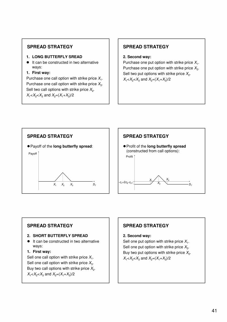
41
SPREAD STRATEGY
1. LONG BUTTERFLY SREAD
� It can be constructed in two alternative ways:
1. First way:
Purchase one call option with strike price X1.
Purchase one call option with strike price X3.
Sell two call options with strike price X2.
X1<X2<X3 and X2=(X1+X3)/2
SPREAD STRATEGY
2. Second way:
Purchase one put option with strike price X1.
Purchase one put option with strike price X3.
Sell two put options with strike price X2.
X1<X2<X3 and X2=(X1+X3)/2
SPREAD STRATEGY
�Payoff of the long butterfly spread:
X1 X2 X3 ST
Payoff
SPREAD STRATEGY
�Profit of the long butterfly spread (constructed from call options):
X1X2
X3
ST
Profit
-c1+2c2-c3
SPREAD STRATEGY
2. SHORT BUTTERFLY SPREAD
� It can be constructed in two alternative ways:
1. First way:
Sell one call option with strike price X1.
Sell one call option with strike price X3.
Buy two call options with strike price X2.
X1<X2<X3 and X2=(X1+X3)/2
SPREAD STRATEGY
2. Second way:
Sell one put option with strike price X1.
Sell one put option with strike price X3.
Buy two put options with strike price X2.
X1<X2<X3 and X2=(X1+X3)/2
42
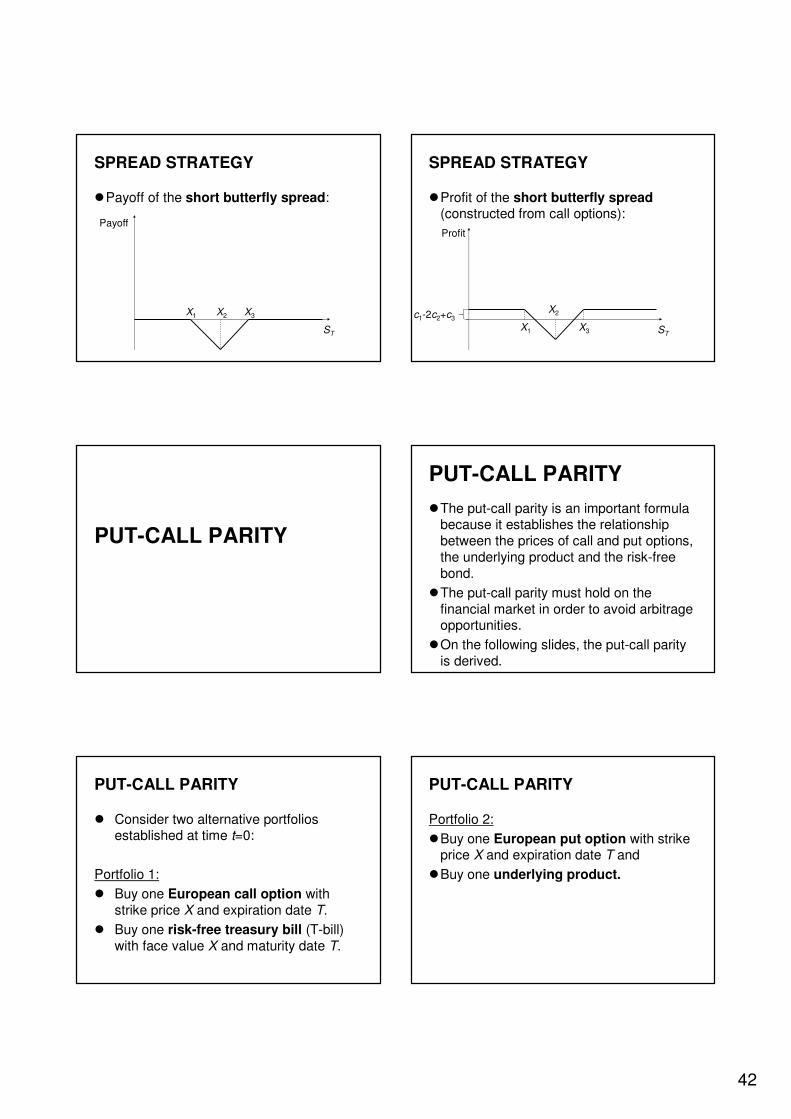
SPREAD STRATEGY
�Payoff of the short butterfly spread:
X1 X2 X3
ST
Payoff
SPREAD STRATEGY
�Profit of the short butterfly spread (constructed from call options):
X1
X2
X3 ST
Profit
c1-2c2+c3
PUT-CALL PARITY
PUT-CALL PARITY
�The put-call parity is an important formula because it establishes the relationship between the prices of call and put options, the underlying product and the risk-free bond.
�The put-call parity must hold on the financial market in order to avoid arbitrage opportunities.
�On the following slides, the put-call parity is derived.
PUT-CALL PARITY
� Consider two alternative portfolios established at time t=0:
Portfolio 1:
� Buy one European call option with strike price X and expiration date T.
� Buy one risk-free treasury bill (T-bill) with face value X and maturity date T.
PUT-CALL PARITY
Portfolio 2:
�Buy one European put option with strike price X and expiration date T and
�Buy one underlying product.

43
PUT-CALL PARITY
�Notice that the payoff of both portfolios at time T is equal independently of ST:
X
X
Payoff
ST
PUT-CALL PARITY
� If the payoff of the portfolios is equal at time T then the cost of establishment of the two portfolios at time t=0 should be equal as well.
�The cost of Portfolio 1 =
c + PV(X) = c + X/(1+r)T
�The cost of Portfolio 2 =
p + S0
PUT-CALL PARITY
�The consequence is that
c + X/(1+r)T = p + S0
or
c + PV(X) = p + S0
�This equation explains the relationship between the prices of the call and put options and is called PUT-CALL PARITY.
PUT-CALL PARITY with dividends
�More general formulation of the put-call parity for dividend paying stocks:
�Suppose that the underlying product is a stock that pays dividends, DIV until the expiration date T.
�Then, we can reformulate the put-call parity as follows:
c + PV(X) + PV(DIV)= p + S0
PUT-CALL PARITY with dividends
Proof:
�Consider two alternative portfolios at time t=0:
Portfolio 1:
�Buy one European call option with strike price X and expiration date T.
�Buy one risk-free treasury bill (T-bill) with face value (X+DIV) and maturity date T.
PUT-CALL PARITY with dividends
Portfolio 2:
�Buy one European put option with strike price X and expiration date T and
�Buy one underlying product.
44
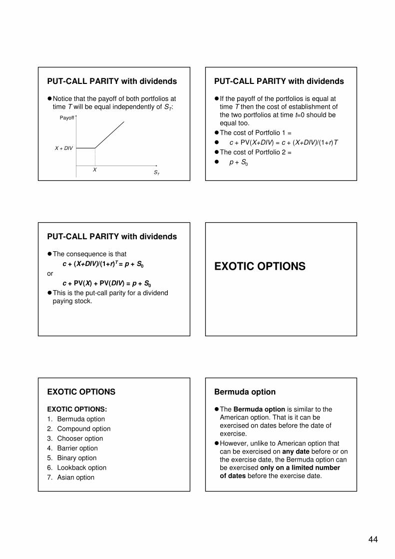
PUT-CALL PARITY with dividends
�Notice that the payoff of both portfolios at time T will be equal independently of ST:
X
X + DIV
Payoff
ST
PUT-CALL PARITY with dividends
� If the payoff of the portfolios is equal at time T then the cost of establishment of the two portfolios at time t=0 should be equal too.
�The cost of Portfolio 1 =
� c + PV(X+DIV) = c + (X+DIV)/(1+r)T
�The cost of Portfolio 2 =
� p + S0
PUT-CALL PARITY with dividends
�The consequence is that
c + (X+DIV)/(1+r)T = p + S0
or
c + PV(X) + PV(DIV) = p + S0
�This is the put-call parity for a dividend paying stock.
EXOTIC OPTIONS
EXOTIC OPTIONS
EXOTIC OPTIONS:
1. Bermuda option
2. Compound option
3. Chooser option
4. Barrier option
5. Binary option
6. Lookback option
7. Asian option
Bermuda option
�The Bermuda option is similar to the American option. That is it can be exercised on dates before the date of exercise.
�However, unlike to American option that can be exercised on any date before or on the exercise date, the Bermuda option can be exercised only on a limited number of dates before the exercise date.

45
Compound option
� The compound option is an option whose underlying product is an option.
� There are four types of compound option:
1. Call option on a call option (underlying = call option)
2. Put option on a call option (underlying = call option)
3. Call option on a put option (underlying = put option)
4. Put option on a put option (underlying = put option)
Chooser option
� In the “chooser” or “as you like it” option, the buyer of the option can choose between having a call option OR a putoption after buying the option.
Barrier option
�Barrier options have payoffs that depend not only on some asset price on the expiration date, but also on whether the underlying asset price has crossed through some “barrier”.
�A barrier option is a type of option where the option to exercise depends on the underlying crossing or reaching a given barrier level.
Barrier option
�Barrier options are always cheaper than a similar option without barrier.
�Therefore, barrier options were created to provide the insurance value of an option without charging as much premium.
Barrier option
There are four types of barrier options:
1. Up-and-out: the price of the underlying starts below the barrier level and has to move up to the barrier level to be knocked out.
2. Down-and-out: the price of the underlying starts above the barrier level and has to move down to the barrier level to be knocked out.
Up-and-out barrier call option
St
t
tSt
Payoff:
max {ST – X,0}
Payoff:
As the barrier has been crossed before t=T, the call option has been knocked out thus its payoff is zero.
Barrier
Barrier
T
T

46
Down-and-out barrier call option
St
t
tSt
Payoff:
max {ST – X,0}
Payoff:
As the barrier has been crossed before t=T, the call option has been knocked out thus its payoff is zero.
Barrier
Barrier
T
T
Barrier option
3. Up-and-in: the price of the underlying starts below the barrier level and has to move up to the barrier level to become activated.
4. Down-and-in: the price of the underlying starts above the barrier level and has to move down to the barrier level to become activated.
Up-and-in barrier call option
St
t
tSt
Payoff:As the barrier has not been crossed before t=T, the call option has not become activated thus its payoff is zero.
Payoff:
The barrier has been passed thus the option has been activated:
max {ST – X,0}
Barrier
Barrier
T
T
Down-and-in barrier call option
St
t
tSt
Payoff:As the barrier has not been crossed before t=T, the call option has not become activated thus its payoff is zero.
Payoff:The barrier has been passed thus the option has been activated:max {ST – X,0}
Barrier
Barrier
T
T
Binary option
�The binary option is an option with discontinuous payoff.
�An example of the binary option is the “cash-or-nothing call”. This option pays nothing if ST<X and pays a fixed cash Q if ST≥X.
ST
X
Q
Payoff
Lookback option
�Lookback options have payoffs that depend in part on the minimum or maximum price of the underlying asset during the live of the option.
�For example, the payoff of a lookback call option may depend on the maximum price:
Payoff = max{max{St}-X,0}
or the minimum price of the underlying asset:
Payoff = max{min{St}-X,0}
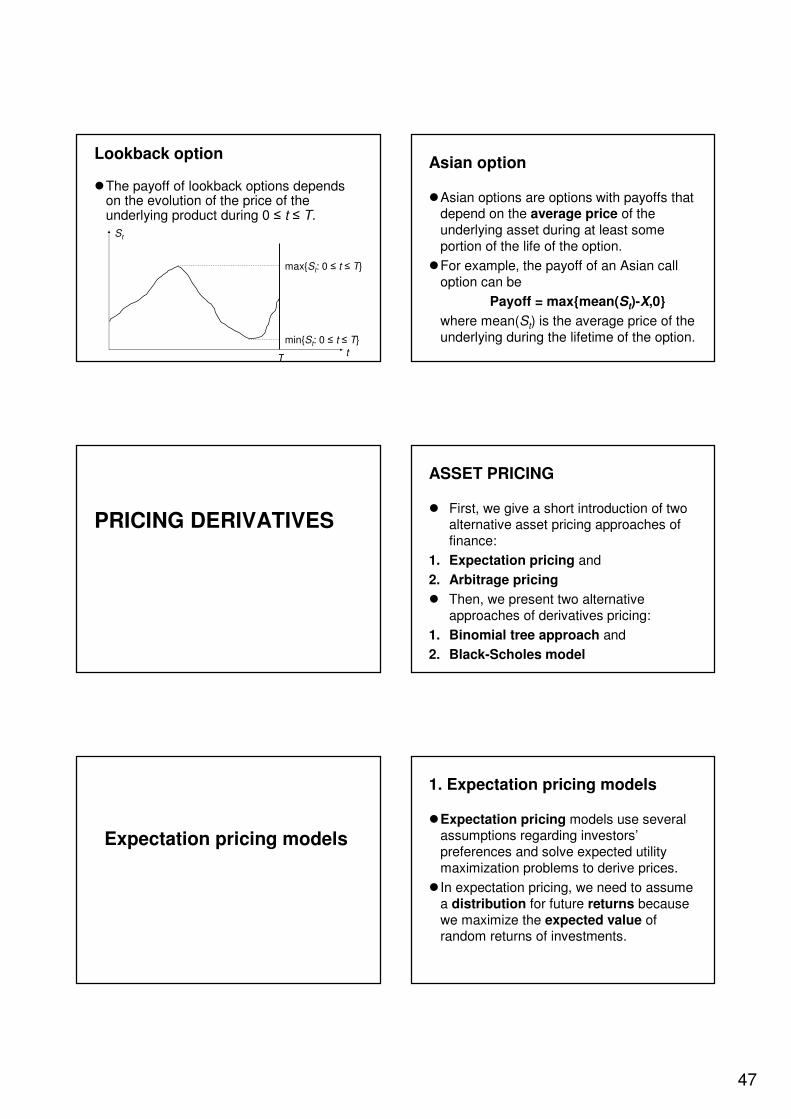
47
Lookback option
�The payoff of lookback options depends on the evolution of the price of the underlying product during 0 ≤ t ≤ T.
Tt
max{St: 0 ≤ t ≤ T}
min{St: 0 ≤ t ≤ T}
St
Asian option
�Asian options are options with payoffs that depend on the average price of the underlying asset during at least some portion of the life of the option.
�For example, the payoff of an Asian call option can be
Payoff = max{mean(St)-X,0}
where mean(St) is the average price of the underlying during the lifetime of the option.
PRICING DERIVATIVES
ASSET PRICING
� First, we give a short introduction of two alternative asset pricing approaches of finance:
1. Expectation pricing and
2. Arbitrage pricing
� Then, we present two alternative approaches of derivatives pricing:
1. Binomial tree approach and
2. Black-Scholes model
Expectation pricing models
1. Expectation pricing models
�Expectation pricing models use several assumptions regarding investors’preferences and solve expected utility maximization problems to derive prices.
� In expectation pricing, we need to assume a distribution for future returns because we maximize the expected value of random returns of investments.
48
1. Expectation pricing models
�This assumption may fail easily and thus the prices obtained by expectation pricing are not robust in general.
�Expectation pricing does not enforcemarket prices, it only gives a suggestionfor market prices.
�A famous equilibrium pricing model is the capital asset pricing model (CAPM).
Arbitrage pricing models
2. Arbitrage pricing models
�An alternative approach is arbitrage pricing, where we do not assume anything about the ‘real world’ probability distribution of future returns.
�Arbitrage pricing is more frequently used in practice then expectation pricing.
�Arbitrage pricing enforces market prices therefore it is a more robust pricing result.
Arbitrage
�Definition (arbitrage opportunity): An arbitrage opportunity arises when the investor can construct a zero investment portfolio that will yield a sure profit.
� In other words, the exploitation of security mispricing in such a way that risk-free economic profits may be earned is called arbitrage.
Arbitrage
� It involves the simultaneous purchase and sale of equivalent securities in order to profit from discrepancies in their price relationship, and so it is an extension of the law of one price.
�The concept of arbitrage is central to the theory of financial markets.
Arbitrage
�Assumption: In order to be able to construct a zero investment portfolio, one has to be able to sell short at least one asset and use the proceeds to purchase (to go long on) one or more assets.
�Borrowing may be considered as a short position in the risk-free asset.
�Even a small investor using short positions can take a large dollar / euro position in such a portfolio.
49
Arbitrage
�A critical property of a risk-free arbitrage portfolio is that any investor, regardless of risk aversion or wealth, will want to take an infinite position in it so that profits will be driven to an infinite level.
�Because those large positions will force prices up or down until the opportunity vanishes, we can derive restrictions on security prices that satisfy the condition that no arbitrage opportunities are left in the marketplace.
Difference between arbitrage and expectation arguments
�Expectation pricing builds on investors’opinion about future returns, while arbitrage pricing uses the price discrepancies among different assets.
�Therefore, we may say that expectation pricing leads to “absolute prices” and arbitrage pricing derives “relative prices”.
Difference between arbitrage and expectation arguments
�There is another important difference between arbitrage and expectation arguments in support of equilibrium price relationships.
�When an expectation argument holds on the market and the equilibrium price relationship is violated, many investors will make portfolio changes.
Difference between arbitrage and expectation arguments
� In an expectation pricing model, each individual investor will make a limited change, though, depending on his or her degree of risk aversion.
�Aggregation of these limited portfolio changes over many investors is required to create a large volume of buying or selling, which in turn restores equilibrium prices.
Difference between arbitrage and expectation arguments
�However, when arbitrage opportunities exist, each investor wants to take as large position as possible.
�Therefore, it will not take many investors to bring about price pressures necessary to restore equilibrium.
�For this reason, implications for prices derived from no-arbitrage arguments are stronger than implications derived from a risk-versus-return dominance argument.
DERIVATIVES PRICING
50
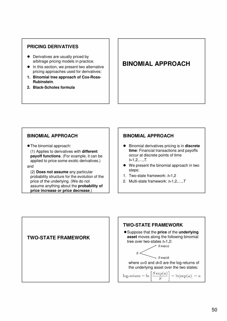
PRICING DERIVATIVES
� Derivatives are usually priced by arbitrage pricing models in practice.
� In this section, we present two alternative pricing approaches used for derivatives:
1. Binomial tree approach of Cox-Ross-Rubinstein.
2. Black-Scholes formula
BINOMIAL APPROACH
BINOMIAL APPROACH
�The binomial approach:
(1) Applies to derivatives with different payoff functions. (For example, it can be applied to price some exotic derivatives.)
and
(2) Does not assume any particular probability structure for the evolution of the price of the underlying. (We do not assume anything about the probability of price increase or price decrease.)
BINOMIAL APPROACH
� Binomial derivatives pricing is in discrete time: Financial transactions and payoffs occur at discrete points of time t=1,2,…,T.
� We present the binomial approach in two steps:
1. Two-state framework: t=1,2
2. Multi-state framework: t=1,2,…,T
TWO-STATE FRAMEWORK
TWO-STATE FRAMEWORK
�Suppose that the price of the underlying asset moves along the following binomial tree over two-states t=1,2:
S
S exp(d)
S exp(u)
where u>0 and d<0 are the log-returns of the underlying asset over the two states:
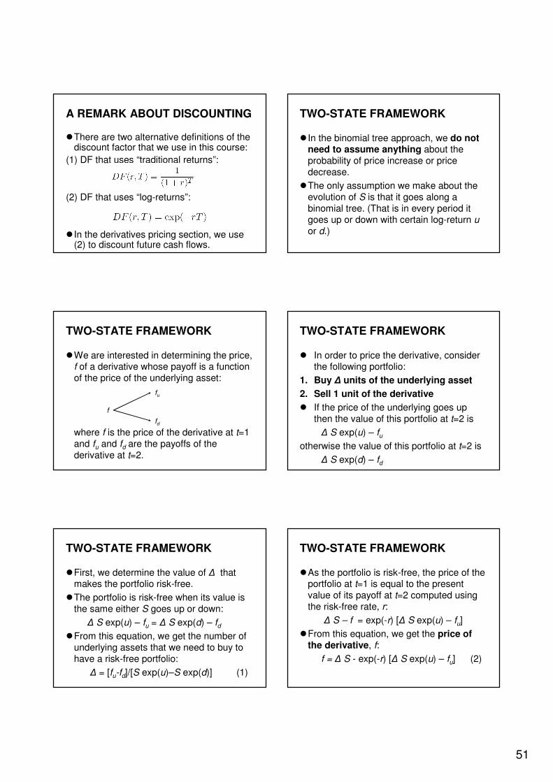
51
A REMARK ABOUT DISCOUNTING
�There are two alternative definitions of the discount factor that we use in this course:
(1) DF that uses “traditional returns”:
(2) DF that uses “log-returns”:
� In the derivatives pricing section, we use (2) to discount future cash flows.
TWO-STATE FRAMEWORK
� In the binomial tree approach, we do not need to assume anything about the probability of price increase or price decrease.
�The only assumption we make about the evolution of S is that it goes along a binomial tree. (That is in every period it goes up or down with certain log-return uor d.)
TWO-STATE FRAMEWORK
�We are interested in determining the price, f of a derivative whose payoff is a function of the price of the underlying asset:
where f is the price of the derivative at t=1 and fu and fd are the payoffs of the derivative at t=2.
fu
fd
f
TWO-STATE FRAMEWORK
� In order to price the derivative, consider the following portfolio:
1. Buy ∆ units of the underlying asset
2. Sell 1 unit of the derivative
� If the price of the underlying goes up then the value of this portfolio at t=2 is
∆ S exp(u) – fuotherwise the value of this portfolio at t=2 is
∆ S exp(d) – fd
TWO-STATE FRAMEWORK
�First, we determine the value of ∆ that makes the portfolio risk-free.
�The portfolio is risk-free when its value is the same either S goes up or down:
∆ S exp(u) – fu = ∆ S exp(d) – fd�From this equation, we get the number of
underlying assets that we need to buy to have a risk-free portfolio:
∆ = [fu-fd]/[S exp(u)–S exp(d)] (1)
TWO-STATE FRAMEWORK
�As the portfolio is risk-free, the price of the portfolio at t=1 is equal to the present value of its payoff at t=2 computed using the risk-free rate, r:
∆ S – f = exp(-r) [∆ S exp(u) – fu]
�From this equation, we get the price of the derivative, f:
f = ∆ S - exp(-r) [∆ S exp(u) – fu] (2)

52
TWO-STATE FRAMEWORK
�We can get an alternative formula for the price of the derivative, f in the following way:
�Substitute (1) into (2). Then, we get:
f = exp(-r) [p fu + (1-p) fd] (3)
where p is defined as
(4)
TWO-STATE FRAMEWORK
�Suppose that d ≤ r ≤ u. (This is a reasonable assumption because d is negative, r is the risk-free rate and u is the rate of the risky underlying asset.)
�Then, it follows from equation (4) that 0 ≤ p ≤ 1.
�Therefore, p can be interpreted as aprobability.
TWO-STATE FRAMEWORK
� If we interpret p in equation (4) as the probability that the price of S goes up then equation (3) has a clear meaning:
�The price of the derivative is the present value, discounted by the risk-free rate, of the expected payoff of the derivative, where the expected value is computed using the probabilities p and (1-p).
TWO-STATE FRAMEWORK
�This pricing approach is very important in derivatives pricing.
� It is called risk-neutral pricing and the probability p is called risk-neutral probability.
TWO-STATE FRAMEWORK
�Remark: Risk neutral pricing has nothing to do with expectation pricing because in risk neutral pricing we use risk neutral probabilities to compute the expected payoff of the derivative whereas in expectation pricing we use the real world probabilities for the same computation.
TWO-STATE FRAMEWORK
� It is important to understand that the price of the derivative we have already obtained in equation (2) before introducing the concept of the risk-neutral probability.
�Then, why did we introduce risk-neutral probability?
�Because equation (3) has a more clear and intuitive meaning than (2): The price of the derivative is the present value of its expected payoff.
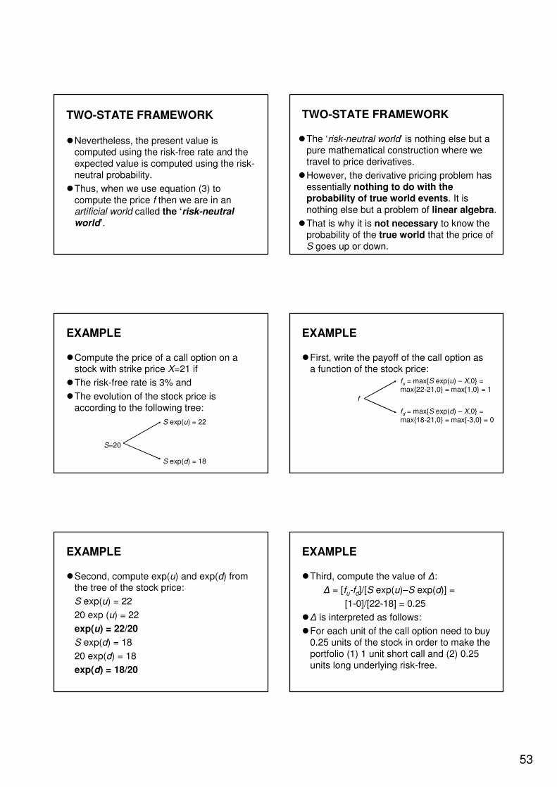
53
TWO-STATE FRAMEWORK
�Nevertheless, the present value is computed using the risk-free rate and the expected value is computed using the risk-neutral probability.
�Thus, when we use equation (3) to compute the price f then we are in an artificial world called the ‘risk-neutral world’.
TWO-STATE FRAMEWORK
�The ‘risk-neutral world’ is nothing else but a pure mathematical construction where we travel to price derivatives.
�However, the derivative pricing problem has essentially nothing to do with the probability of true world events. It is nothing else but a problem of linear algebra.
�That is why it is not necessary to know the probability of the true world that the price of S goes up or down.
EXAMPLE
�Compute the price of a call option on a stock with strike price X=21 if
�The risk-free rate is 3% and
�The evolution of the stock price is according to the following tree:
S=20
S exp(u) = 22
S exp(d) = 18
EXAMPLE
�First, write the payoff of the call option as a function of the stock price:
f
fu = max{S exp(u) – X,0} = max{22-21,0} = max{1,0} = 1
fd = max{S exp(d) – X,0} = max{18-21,0} = max{-3,0} = 0
EXAMPLE
�Second, compute exp(u) and exp(d) from the tree of the stock price:
S exp(u) = 22
20 exp (u) = 22
exp(u) = 22/20
S exp(d) = 18
20 exp(d) = 18
exp(d) = 18/20
EXAMPLE
�Third, compute the value of ∆:
∆ = [fu-fd]/[S exp(u)–S exp(d)] =
[1-0]/[22-18] = 0.25
�∆ is interpreted as follows:
�For each unit of the call option need to buy 0.25 units of the stock in order to make the portfolio (1) 1 unit short call and (2) 0.25 units long underlying risk-free.
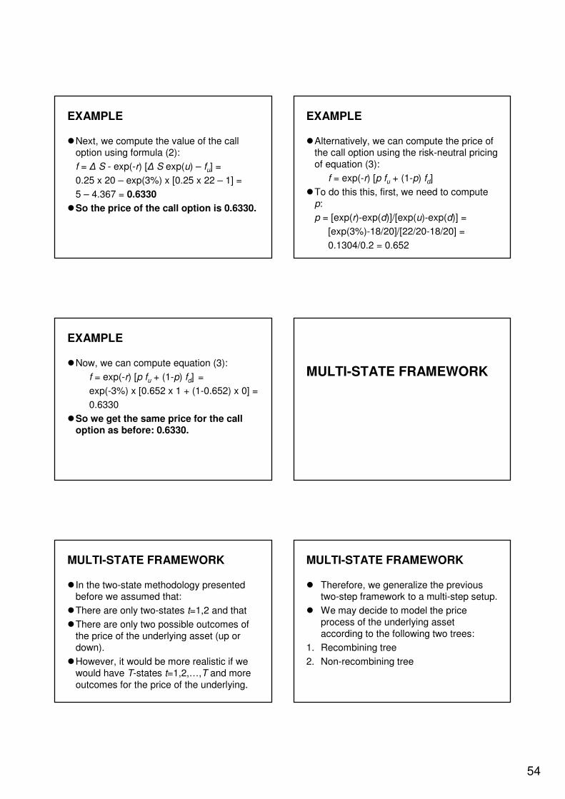
54
EXAMPLE
�Next, we compute the value of the call option using formula (2):
f = ∆ S - exp(-r) [∆ S exp(u) – fu] =
0.25 x 20 – exp(3%) x [0.25 x 22 – 1] =
5 – 4.367 = 0.6330
�So the price of the call option is 0.6330.
EXAMPLE
�Alternatively, we can compute the price of the call option using the risk-neutral pricing of equation (3):
f = exp(-r) [p fu + (1-p) fd]
�To do this this, first, we need to compute p:
p = [exp(r)-exp(d)]/[exp(u)-exp(d)] =
[exp(3%)-18/20]/[22/20-18/20] =
0.1304/0.2 = 0.652
EXAMPLE
�Now, we can compute equation (3):
f = exp(-r) [p fu + (1-p) fd] =
exp(-3%) x [0.652 x 1 + (1-0.652) x 0] =
0.6330
�So we get the same price for the call option as before: 0.6330.
MULTI-STATE FRAMEWORK
MULTI-STATE FRAMEWORK
� In the two-state methodology presented before we assumed that:
�There are only two-states t=1,2 and that
�There are only two possible outcomes of the price of the underlying asset (up or down).
�However, it would be more realistic if we would have T-states t=1,2,…,T and more outcomes for the price of the underlying.
MULTI-STATE FRAMEWORK
� Therefore, we generalize the previous two-step framework to a multi-step setup.
� We may decide to model the price process of the underlying asset according to the following two trees:
1. Recombining tree
2. Non-recombining tree

55
MULTI-STATE FRAMEWORKRECOMBINING TREE
Notice that on this figure t=1,…,4 and the number of possible outcomes is 4.
MULTI-STATE FRAMEWORKNON-RECOMBINING TREE
Notice that on this figure t=1,…,4 and the number of possible outcomes is 8.
MULTI-STATE FRAMEWORK
�We can see that the non-recombining tree allows more outcomes, i.e. it is more general.
�The pricing approach to be discussed applies to both types of trees.
�However, it is computationally easier to work with the recombining tree.
� In the followings, we focus on the recombining tree to compute prices.
MULTI-STATE FRAMEWORK
Notice that the multi-state tree is simply the sum of two-state trees.
MULTI-STATE FRAMEWORK
� If we think of the multi-state tree as the sum of several two-state trees then we can easily apply the approach introduced in the two-state slides for the multi-state tree.
�To show how to do it in practice we consider three states:
MULTI-STATE FRAMEWORK
�This is the tree of prices of the underlying asset.
S exp(2u)
S exp(u+d)
S exp(2d)
S exp(u)
S exp(d)
S

56
MULTI-STATE FRAMEWORK
�This is the tree of prices and payoffs of the derivative to be priced.
fuu
fud = fdu
fdd
fu
fd
f
MULTI-STATE FRAMEWORK
�The objective is to determine the value f.
�We do it backward: we start with the last nodes of the tree. (See the upper right box on the graph).
fuu
fud = fdu
fdd
fu
fd
f
MULTI-STATE FRAMEWORK
� In the first step, we determine the payoffs fuu and fud of the last state.
�Then, we use the two-state framework to compute the value fu.
fuu
fud = fdu
fdd
fu
fd
f
MULTI-STATE FRAMEWORK
�Then, we focus on the lower right rectangle of the figure. (See on the graph.)
fuu
fud = fdu
fdd
fu
fd
f
MULTI-STATE FRAMEWORK
� In the second step, we determine the payoffs fud and fdd of the last state.
�Then, we use the two-state framework to compute the value fd.
fuu
fud = fdu
fdd
fu
fd
f
MULTI-STATE FRAMEWORK
�Once we have computed fu and fd, we focus on the final rectangle presented on the graph.
fuu
fud = fdu
fdd
fu
fd
f
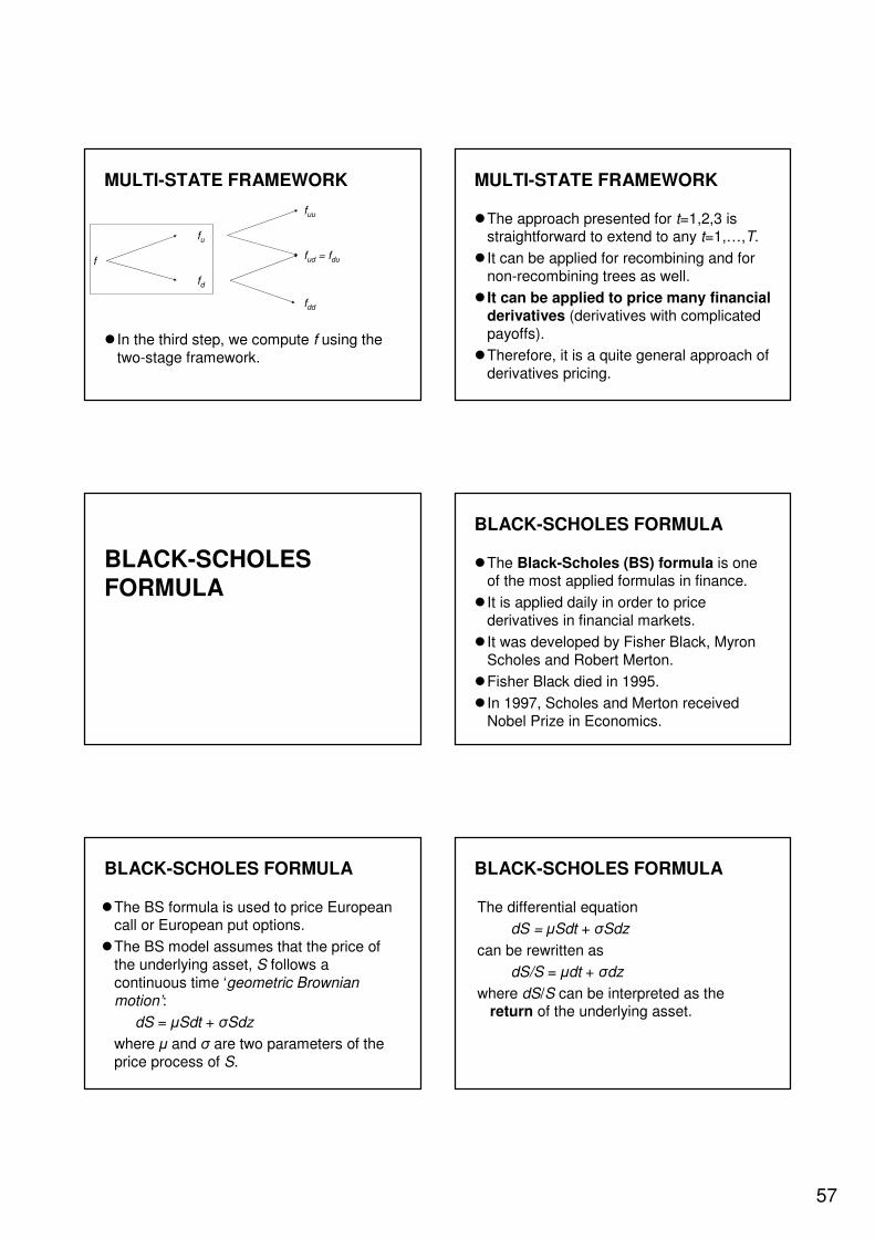
57
MULTI-STATE FRAMEWORK
� In the third step, we compute f using the two-stage framework.
fuu
fud = fdu
fdd
fu
fd
f
�The approach presented for t=1,2,3 is straightforward to extend to any t=1,…,T.
� It can be applied for recombining and for non-recombining trees as well.
� It can be applied to price many financial derivatives (derivatives with complicated payoffs).
�Therefore, it is a quite general approach of derivatives pricing.
MULTI-STATE FRAMEWORK
BLACK-SCHOLES FORMULA
BLACK-SCHOLES FORMULA
�The Black-Scholes (BS) formula is one of the most applied formulas in finance.
� It is applied daily in order to price derivatives in financial markets.
� It was developed by Fisher Black, Myron Scholes and Robert Merton.
�Fisher Black died in 1995.
� In 1997, Scholes and Merton received Nobel Prize in Economics.
BLACK-SCHOLES FORMULA
�The BS formula is used to price European call or European put options.
�The BS model assumes that the price of the underlying asset, S follows a continuous time ‘geometric Brownian
motion’:
dS = µSdt + σSdz
where µ and σ are two parameters of the price process of S.
BLACK-SCHOLES FORMULA
The differential equation
dS = µSdt + σSdz
can be rewritten as
dS/S = µdt + σdz
where dS/S can be interpreted as the return of the underlying asset.

58
BLACK-SCHOLES FORMULA
� Two components of the return process:
1. µdt is the deterministic trendcomponent with slope µ and
2. σdz is the random noise component with standard deviation σ.
� Therefore, the return process is simply a noise around a deterministic trend.
� To present this, we graph the return process described by dS/S = µdt + σdzas follows:
Components of the
geometric Brownian motion
-10
-5
0
5
10
15
20
1 6 11 16 21 26 31 36 41 46 51 56 61 66 71 76 81 86 91 96 101
time
σdz
µdt
µdt + σdz
BLACK-SCHOLES FORMULA
� Notice that:
(1) BS assumes a particular ‘real world’probability structure of the price process S,
(2) the BS model is formulated in continuous time, and
(3) the BS formula applies only to a limited number of derivatives: European call and put options.
BLACK-SCHOLES FORMULA
�The BS price of a European call option:
BLACK-SCHOLES FORMULA
Notation:
� S0: price of the underlying asset at t=0.
� X: strike price of the option.
� r : risk-free rate.
� T: time-to-expiration of the option.
� σ : standard deviation of the return of the underlying asset (“volatility”).
� N(·): cumulative distribution function of the standard normal distribution.
BLACK-SCHOLES FORMULA
� The BS price of a European put option:

59
BLACK-SCHOLES FORMULA
Notation:
� S0: price of the underlying asset at t=0.
� X: strike price of the option.
� r : risk-free rate.
� T: time-to-expiration of the option.
� σ : standard deviation of the return of the underlying asset (“volatility”).
� N(·): cumulative distribution function of the standard normal distribution.
A REMARK ABOUT TIME SCALE
�Notice that the
(1) risk-free rate, r
(2) time-to-expiration, T and
(3) volatility, σ
are time scale dependent variables.
� In the BS formula, one needs to use annual scale for these variables. (annualrisk-free rate; T measured in years and standard deviation of annual returns, σ.
A REMARK ABOUT VOLATILITY
�Notice that in the BS formula one of the parameters is volatility of the return of the underlying asset.
�However, the slope of the deterministic trend, µ is not in the formula.
�The presence of σ in the BS formula means that the ‘real world’ probability structure of the underlying price process influences the BS option price.
�Remember that in the binomial tree approach it is not like this!!!
VOLATILITY ESTIMATION
Annual volatility estimation
� In the BS formula, we need the volatility of annual returns.
�However, consistent estimation of σ from annual data series is not possible due to small sample size.
Annual volatility estimation
�One solution is to use a higher frequency data, for example daily returns,
(1) Estimate volatility of daily returns, then,
(2) Rescale daily volatility to annual volatility.
�We can do this in the following way:
60
Annual volatility estimation
Suppose that:
� (1) We estimate daily volatility, σ1day as follows:
where yt is daily return, is the mean of yt and n is the sample size.
� (2) There are 250 trading days during a year.
� (3) Daily returns are independent random variables.
Annual volatility estimation
�Then, the annual volatility can be rescaled from daily volatility as follows:
Advantages of this methodology:
(1) The sample size can be large, therefore the statistical estimation is reliable.
(2) We use ‘relatively recent’ return data to estimate annual volatility.
Annual volatility estimation
�Disadvantage of this methodology:
�Daily returns are not independent random variables!
�There exist more sophisticated dynamic models of volatility showing this fact. (See the GARCH model for example).
COMPUTING THE VALUE OF N(·)
A REMARK ABOUT N(·)
�The cumulative distribution of N(0,1) is given in tables.
�See the table of N(·) left in the copy shop.
�Be familiar about how to obtain a value of N(x) based on that table!
� In Excel, there is a function for the cumulative distribution function of N(0,1):
�NORMSDIST(x) - in English Excel
�DISTR.NORM.ESTAND(x) – in Spanish Excel
EXERCISE OF N(·)
�See the table for using the table for x ≥ 0:
N(0.6278) =
= N(0.62) + 0.78[N(0.63) – N(0.62)]
= 0.7324 + 0.78x(0.7357 – 0.7324)
= 0.7350
61
EXERCISE OF N(·)
�See the table for using the table for x ≤ 0:
N(-0.1234)=
= N(-0.12) – 0.34[N(-0.12) – N(-0.13)]
= 0.4522 – 0.34x(0.4522 – 0.4483)
= 0.4509
EXERCISE OF N(·)
�Use the table of the N(0,1) distribution to compute N(x) for the next values of x:
(a) x = 0.0521
(b) x = 0.1367
(c) x = 2.4701
(d) x = -0.0012
(e) x = -1.5419
(f) x = -2.3177
(a) x = 0.0521
�N(0.0521) =
N(0.05) + 0.21[N(0.06) - N(0.05)] =
0.5199 + 0.21[0.5239 – 0.5199] =
0.5207
(b) x = 0.1367
�N(0.1367) =
N(0.13) + 0.67[N(0.14) – N(0.13)] =
0.5517 + 0.67[0.5557 – 0.5517] =
0.5544
(c) x = 2.4701
�N(2.4701)=
N(2.47) + 0.01[N(2.48)-N(2.47)] =
0.9932 + 0.01[0.9934 – 0.9932] =
0.9932
(d) x = -0.0012
�N(-0.0012)=
N(-0.00) – 0.12[N(-0.00) – N(-0.01)] =
0.5 – 0.12[0.5 – 0.4960] =
0.4995
62
(e) x = -1.5419
�N(-1.5419) =
N(-1.54) - 0.19[N(-1.54) – N(-1.55)] =
0.0618 – 0.19[0.0618 – 0.0606] =
0.0616
(f) x = -2.3177
�N(-2.3177) =
N(-2.31) – 0.77[N(-2.31) – N(-2.32)] =
0.0104 – 0.77[0.0104 – 0.0102] =
0.0102
RISK MANAGEMENT OF OPTIONS CONTRACTS
RISK MANAGEMENT OF OPTIONS
� In the previous section, we priced options in a static setup:
�We computed the price of derivatives at time t = 0.
�However, in the reality we are in a dynamic setup: t = 0,...,T.
�This means that investors are interested in the evolution of the prices in their portfolios over time.
RISK MANAGEMENT OF OPTIONS
� In this section, we are going to analyze to risks associated to European optioncontracts in the BS framework.
�Remember from the BS formulas that the price of an option is determined by the next five elements:
RISK MANAGEMENT OF OPTIONS
1. Strike price, X
2. Time to expiration, T
3. Risk-free interest rate, r
4. Spot price of the underlying asset, S0
5. Volatility of the underlying asset return, σ
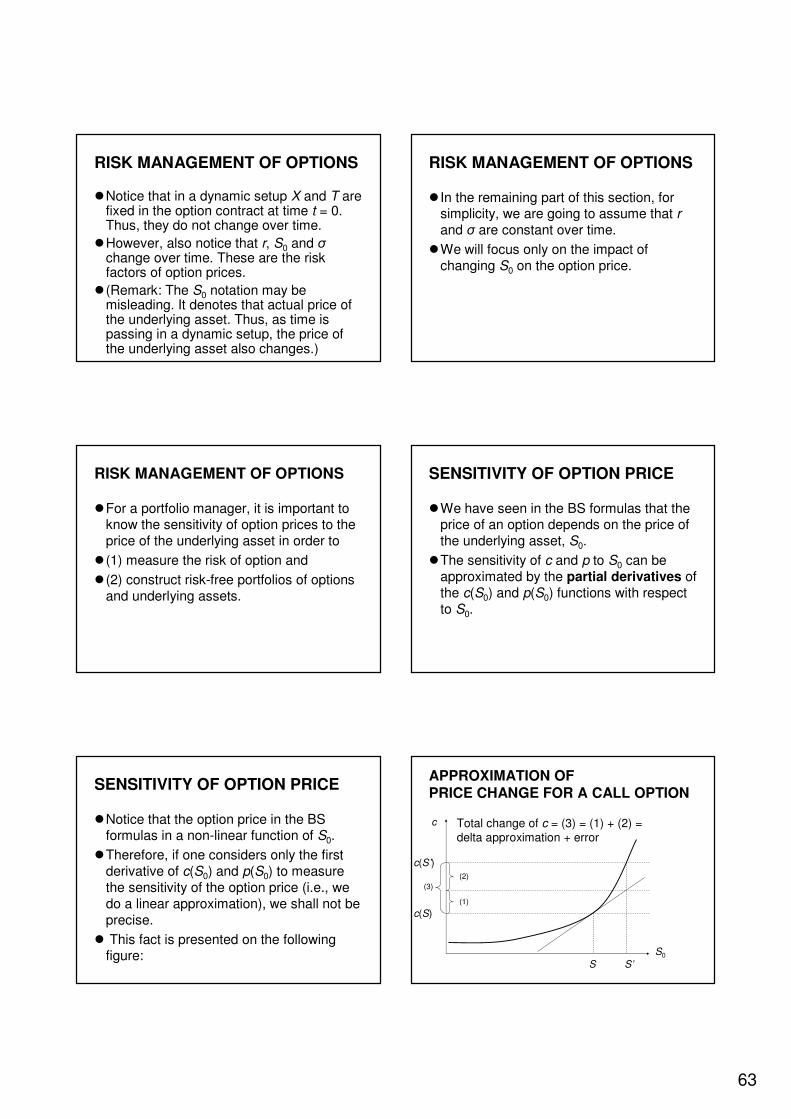
63
RISK MANAGEMENT OF OPTIONS
�Notice that in a dynamic setup X and T are fixed in the option contract at time t = 0. Thus, they do not change over time.
�However, also notice that r, S0 and σchange over time. These are the risk factors of option prices.
� (Remark: The S0 notation may be misleading. It denotes that actual price of the underlying asset. Thus, as time is passing in a dynamic setup, the price of the underlying asset also changes.)
RISK MANAGEMENT OF OPTIONS
� In the remaining part of this section, for simplicity, we are going to assume that rand σ are constant over time.
�We will focus only on the impact of changing S0 on the option price.
RISK MANAGEMENT OF OPTIONS
�For a portfolio manager, it is important to know the sensitivity of option prices to the price of the underlying asset in order to
� (1) measure the risk of option and
� (2) construct risk-free portfolios of options and underlying assets.
SENSITIVITY OF OPTION PRICE
�We have seen in the BS formulas that the price of an option depends on the price of the underlying asset, S0.
�The sensitivity of c and p to S0 can be approximated by the partial derivatives of the c(S0) and p(S0) functions with respect to S0.
SENSITIVITY OF OPTION PRICE
�Notice that the option price in the BS formulas in a non-linear function of S0.
�Therefore, if one considers only the first derivative of c(S0) and p(S0) to measure the sensitivity of the option price (i.e., we do a linear approximation), we shall not be precise.
� This fact is presented on the following figure:
APPROXIMATION OF PRICE CHANGE FOR A CALL OPTION
S0
c
S’S
Total change of c = (3) = (1) + (2) = delta approximation + error
(3)
(1)
(2)
c(S)
c(S’)
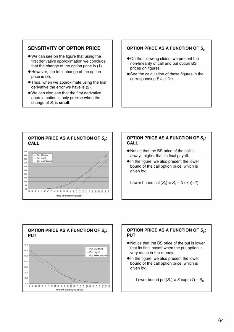
64
SENSITIVITY OF OPTION PRICE
�We can see on the figure that using the first derivative approximation we conclude that the change of the option price is (1).
�However, the total change of the option price is (3).
�Thus, when we approximate using the first derivative the error we have is (2).
�We can also see that the first derivative approximation is only precise when the change of S0 is small.
OPTION PRICE AS A FUNCTION OF S0
�On the following slides, we present the non-linearity of call and put option BS prices on figures.
�See the calculation of these figures in the corresponding Excel file.
0.0
5.0
10.0
15.0
20.0
25.0
30.0
35.0
40.0
45.0
50.0
50
54
58
62
66
70
74
78
82
86
90
94
98
102
106
110
114
118
122
126
130
134
138
142
146
150
Price of underlying asset
Call BS price
Call payoff
Call lower bound
OPTION PRICE AS A FUNCTION OF S0: CALL
OPTION PRICE AS A FUNCTION OF S0: CALL
�Notice that the BS price of the call is always higher that its final payoff.
� In the figure, we also present the lower bound of the call option price, which is given by:
Lower bound call(S0) = S0 – X exp(-rT)
0.0
10.0
20.0
30.0
40.0
50.0
60.0
70.0
50
54
58
62
66
70
74
78
82
86
90
94
98
102
106
110
114
118
122
126
130
134
138
142
146
150
Price of underlying asset
Put BS price
Put payoff
Put lower bound
OPTION PRICE AS A FUNCTION OF S0:
PUT
OPTION PRICE AS A FUNCTION OF S0: PUT
�Notice that the BS price of the put is lower that its final payoff when the put option is very much in-the-money.
� In the figure, we also present the lower bound of the call option price, which is given by:
Lower bound put(S0) = X exp(-rT) – S0
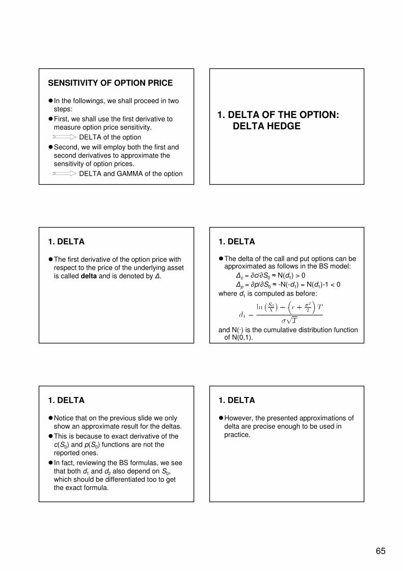
65
SENSITIVITY OF OPTION PRICE
� In the followings, we shall proceed in two steps:
�First, we shall use the first derivative to measure option price sensitivity.
DELTA of the option
�Second, we will employ both the first and second derivatives to approximate the sensitivity of option prices.
DELTA and GAMMA of the option
1. DELTA OF THE OPTION: DELTA HEDGE
1. DELTA
�The first derivative of the option price with respect to the price of the underlying asset is called delta and is denoted by ∆.
1. DELTA
�The delta of the call and put options can be approximated as follows in the BS model:
∆c = ∂c/∂S0 ≈ N(d1) > 0
∆p = ∂p/∂S0 ≈ -N(-d1) = N(d1)-1 < 0
where d1 is computed as before:
and N(·) is the cumulative distribution function of N(0,1).
1. DELTA
�Notice that on the previous slide we only show an approximate result for the deltas.
�This is because to exact derivative of the c(S0) and p(S0) functions are not the reported ones.
� In fact, reviewing the BS formulas, we see that both d1 and d2 also depend on S0, which should be differentiated too to get the exact formula.
1. DELTA
�However, the presented approximations of delta are precise enough to be used in practice.
66
1. DELTA
�Notice that the delta of the call option is positive while the delta of the put option is negative.
�This means that if the price of the underlying product increases then the price of the call option will increase.
� In addition, if the price of the underlying product increases then the price of the put option will decrease.
1. DELTA: CALL OPTION SENSITIVITY
�The change of the call option price in the BS model can be approximated by delta as follows:
where dc = c1-c0 are dS = S1-S0 the changes of the option price and underlying asset price between t = 0 and t = 1, respectively.
1. DELTA: PUT OPTION SENSITIVITY
�The change of the put option price in the BS model can be approximated by delta as follows:
where dp = p1-p0 are dS = S1-S0 the changes of the option price and underlying asset price between t = 0 and t = 1, respectively.
1. DELTA: SENSITIVITY OF OPTION PRICE
�Why is it useful to compute the delta of the option price?
� It is useful because:
� (1) The |∆| can be seen as a risk measure of the option price.
� (2) The |∆| defines the so-called hedge ratio of the option.
1. DELTA: SENSITIVITY OF OPTION PRICE
�The hedge ratio of an option tells us how to construct a delta neutral portfolio from
(1) the underlying asset and
(2) the option.
�When we use the hedge ratio to construct a delta neutral portfolio then we do a so-called delta hedge.
�On the next slides, we consider delta hedge for European call and put options.
1. DELTA HEDGE: CALL OPTION
� Consider the following portfolio:
1. Buy |∆| units of the underlying asset and
2. Sell 1 unit of a call option on the underlying asset.
� This portfolio is not sensitive to smallchanges of the price of the underlying asset.
� (Remember that the price of the call option is increasing in the price of the underlying asset. See previous figure.)
67
1. DELTA HEDGE: PUT OPTION
� Consider the following portfolio:
1. Buy |∆| units of the underlying asset and
2. Buy 1 unit of a put option on the underlying asset.
� This portfolio is not sensitive to smallchanges of the price of the underlying asset.
� (Remember that the price of the put option is decreasing in the price of the underlying asset. See previous figure.)
1. THE DELTA HEDGE RATIO FORMULA
Disadvantage:
�One can hedge only small changes of the underlying asset price.
Advantage:
�The formula includes terms known at time t = 0.
� In other words, the risk manager can compute this hedge ratio using information observed at time t = 0.
1. DELTA HEDGE
�We shall see an example later for the computation of delta and delta hedge.
2. GAMMA OF THE OPTION:DELTA-GAMMA HEDGE
2. GAMMA: MOTIVATION
�As we have seen before, the price of an option is non-linear function of S0 in the BS formulas.
�This means that the first derivative is only a linear approximation of the total change of option price for the change of S0 and works only if the change of S0 is small.
2. GAMMA: MOTIVATION
�A more reliable, non-linear approximation of the sensitivity of option price to S0 is obtained when we take into account the second partial derivative of the option price as well.
�First, we will present how to compute to second derivative, called gamma, of an option in the BS framework.
�Then, we shall approximate the sensitivity of option price using both delta and gamma.
68
2. GAMMA: DEFINITION
�The second derivative of S0 is called gamma and denoted by Γ.
� In the Black-Scholes model, the gammas of call and put options are equal and are computed as follows:
2. GAMMA: DEFINITION
� In the previous formula, N’(d1) denotes the density function of N(0,1), which can be computed as
or in Excel use the following function:
�English: NORMDIST(d1,0,1,FALSE)
�Spanish: DISTR.NORM(d1,0,1,FALSO)
2. DELTA-GAMMA
�On the following slides, we focus on the delta-gamma approximation of option price sensitivity using the first two terms of the Taylor series of c(S0) and p(S0).
2. DELTA-GAMMA: CALL OPTION SENSITIVITY
�Writing the first two terms of the Taylor formula for the c(S0) function we have:
�Substituting the definitions of delta and gamma into this equation we obtain:
2. DELTA-GAMMA: CALL OPTION SENSITIVITY
� In the previous formula, dS is the change of the price of the underlying asset between t = 0 and t = 1:
dS = S1 - S0
�∆ is computed at t = 0
�and Γ is computed at t = 0
�dc is the approximation of the price change of the call option between t = 0 and t = 1:
dc = c1 - c0
2. DELTA-GAMMA: PUT OPTION SENSITIVITY
�Writing the first two terms of the Taylor formula for the p(S0) function we have:
�Substituting the definitions of delta and gamma into this equation we obtain:
69
2. DELTA-GAMMA: PUT OPTION SENSITIVITY
� In the previous formula, dS is the change of the price of the underlying asset between t = 0 and t = 1:
dS = S1 - S0
�∆ is computed at t = 0
�and Γ is computed at t = 0
�dp is the approximation of the price change of the put option between t = 0 and t = 1:
dp = p1 - p0
2. DELTA-GAMMA: OPTION SENSITIVITY
�Substituting the computation of delta and gamma for the call and put options priced by the BS formula, we can write the delta-gamma approximation of call and put options as follows:
2. DELTA-GAMMA: OPTION SENSITIVITY
�Call option:
�Put option:
2. DELTA-GAMMA: SENSITIVITY OF OPTION PRICE
�Why is it useful to compute the gamma of the option price?
� It is useful because:
� (1) The |∆ + 0.5 x Γ x dS| value can be used as an alternative risk measure of the option price.
� (2) The |∆ + 0.5 x Γ x dS| value defines an alternative hedge ratio of the option.
2. ALTERNATIVE HEDGE RATIO
�The formula for the alternative hedge ratio is obtained rewriting the equations of the delta-gamma approximation of the call and put options:
2. DELTA-GAMMA: SENSITIVITY OF OPTION PRICE
�The hedge ratio of an option tells us how to construct a delta-gamma neutral portfolio from
(1) the underlying asset and
(2) the option.
�When we use this alternative hedge ratio to construct a delta-gamma neutral portfolio then we do a so-called delta-gamma hedge.
�On the next slides, we consider delta-gamma hedge for European call and put options.
70
2. DELTA-GAMMA HEDGE: CALL OPTION
� Consider the following portfolio:
1. Buy |∆ + 0.5 x Γ x dS| units of the underlying asset and
2. Sell 1 unit of a call option on the underlying asset.
� This portfolio is not sensitive to largechanges of the price of the underlying asset.
� (Remember that the price of the call option is increasing in the price of the underlying asset.)
2. DELTA-GAMMA HEDGE: PUT OPTION
� Consider the following portfolio:
1. Buy |∆ + 0.5 x Γ x dS| units of the underlying asset and
2. Buy 1 unit of a put option on the underlying asset.
� This portfolio is not sensitive to largechanges of the price of the underlying asset.
� (Remember that the price of the put option is decreasing in the price of the underlying asset.)
2. THE DELTA-GAMMA HEDGE
RATIO FORMULA
Advantage:
�One can hedge large changes of the underlying asset price.
Disadvantage:
�The formula includes the dS=S1-S0 term and S1 is not known at time t = 0.
�Thus, the risk manager needs to suppose a future price for the underlying asset.
OPTION RISK MANAGEMENT: TWO EXAMPLES
�You are a financial risk manager of BBVA.
�You have to
(Ex.1) Compute the delta and gamma of a European call and a European put option and approximate the future change of the option prices using these values.
(Ex.2) Form a delta neutral and a delta-gamma neutral portfolio from the options and their underlying asset.
OPTION RISK MANAGEMENT: TWO EXAMPLES
�On the next slides, we solve these two tasks in examples 1 and 2.
EXAMPLE 1: DELTA-GAMMA APPROXIMATION
(1) Compute the delta and gamma of a European call and a European putoption and approximate the future change of the option prices using these values.

71
EXAMPLE 1: DELTA-GAMMA APPROXIMATION
� In part (1a), the delta and gamma values are computed for European call optionusing the BS model.
� In part (1b), the delta and gamma values are computed for European call put option using the BS model.
(1a) DELTA AND GAMMA COMPUTATION FOR CALL
� The delta and gamma values are computed for European call option using the BS model.
� We shall use the next initial data for both options:
15%15%σ
22T
3%3%r
110110X
105100S
t=1t=0
5dSdS=S1–S0
S0
strike price
risk-free rate
expiration date
volatility
(1a) DELTA AND GAMMA COMPUTATION FOR CALL
�Next, we calculate d1, d2, N(d1), N(d2) and N’(d1):
0.390.40N'(d1)
0.480.39N(d2)
0.570.48N(d1)
-0.04-0.27d2
0.17-0.06d1
t=1t=0
(1a) DELTA AND GAMMA COMPUTATION FOR CALL
� Finally, we compute the values of BS call price, delta, gamma and the corresponding true and approximated changes:
∆- Γ approx.: ∆ds + ½Γ(ds)22.614270.01770.0188Γ
∆ approx.: ∆ds2.379620.56730.4759∆
True change: dc=c1-c02.610509.536.92c
dct=1t=0
(1a) DELTA AND GAMMA COMPUTATION FOR CALL
�Remark: When we compute the approximations in the previous table, we should use the values of delta and gamma for t = 0 (marked by bold letters).
� In other words, we only use current, known values to approximate the option price change.
(1b) DELTA AND GAMMA COMPUTATION FOR PUT
� The delta and gamma values are computed for European call put option using the BS model.
� We shall use the next initial data for both options:
dS=S1–S0
S0
strike price
risk-free rate
expiration date
volatility15%15%σ
22T
3%3%r
110110X
105100S
t=1t=0
5dS

72
(1b) DELTA AND GAMMA COMPUTATION FOR PUT
�Next, we calculate d1, d2, N(d1), N(d2) and N’(d1):
0.390.40N'(d1)
0.520.61N(-d2)
0.430.52N(-d1)
-0.04-0.27d2
0.17-0.06d1
t=1t=0
(1b) DELTA AND GAMMA COMPUTATION FOR PUT
� Finally, we compute the values of BS call price, delta, gamma and the corresponding true and approximated changes:
∆- Γ approx.: ∆ds + ½Γ(ds)2
-2.385730.01770.0188Γ
∆ approx.: ∆ds-2.62038-0.4327-0.5241∆
True change: dp=p1-p0-2.389508.1210.51p
dct=1t=0
(1b) DELTA AND GAMMA COMPUTATION FOR PUT
�Note: Again, when we compute the approximations in the previous table, we should use the values of delta and gamma for t = 0 (marked by bold letters).
� In other words, we only use current, known values to approximate the option price change.
EXAMPLE 2 : DELTA-GAMMA HEDGE
(2) Form a delta neutral and a delta-gamma neutral portfolio from the options and their underlying asset.
EXAMPLE 2: DELTA-GAMMA HEDGE
� In part (2a), we shall consider the hedge of a European short call position by a long underlying asset position.
� In part (2b), we will review the hedge of a European long put position by a long underlying asset position.
� In both parts, we form two alternative portfolios: (*) delta neutral and (**) delta-gamma neutral.
�We use the data from Example 1.
(2a) Hedge of a European short call position by a long underlying asset position
(*) The next table presents a delta neutral portfolio:
-0.2309PORTFOLIO
2.37960.4759|∆|long underlying asset
-2.6105-1-1short call
true changeunitsunitsasset
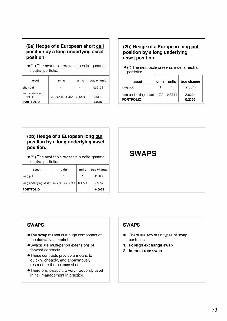
73
� (**) The next table presents a delta-gamma neutral portfolio:
0.0038PORTFOLIO
2.61430.5229|∆ + 0.5 x Γ x dS|long underlying
asset
-2.6105-1-1short call
true changeunitsunitsasset
(2a) Hedge of a European short callposition by a long underlying asset position
(2b) Hedge of a European long putposition by a long underlying asset position.
� (*) The next table presents a delta neutral portfolio:
0.2309PORTFOLIO
2.62040.5241|∆|long underlying asset
-2.389511long put
true changeunitsunitsasset
� (**) The next table presents a delta-gamma neutral portfolio:
-0.0038PORTFOLIO
2.38570.4771|∆ + 0.5 x Γ x dS|long underlying asset
-2.389511long put
true changeunitsunitsasset
(2b) Hedge of a European long putposition by a long underlying asset position.
SWAPS
SWAPS
�The swap market is a huge component of the derivatives market.
�Swaps are multi-period extensions of forward contracts.
�These contracts provide a means to quickly, cheaply, and anonymously restructure the balance sheet.
�Therefore, swaps are very frequently used in risk management in practice.
SWAPS
� There are two main types of swap contracts:
1. Foreign exchange swap
2. Interest rate swap
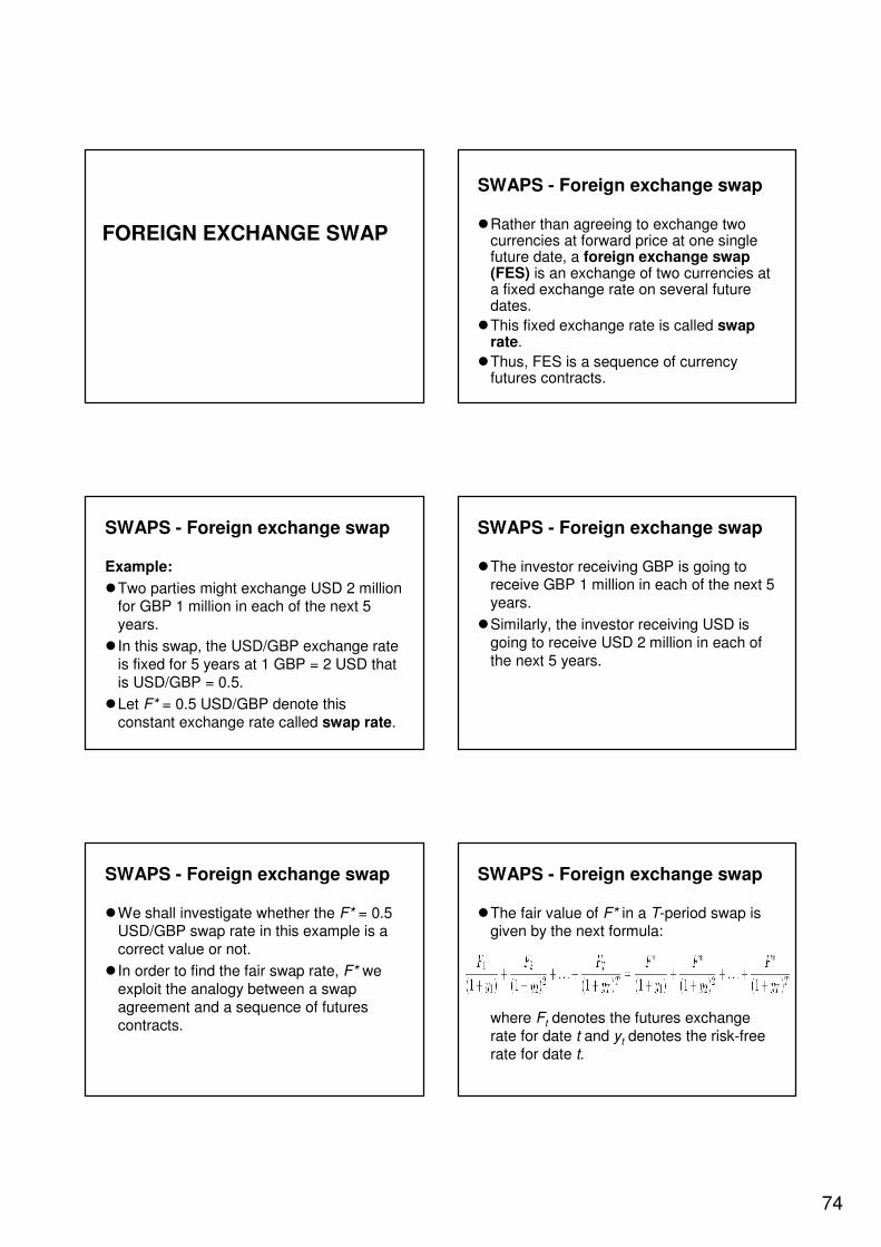
74
FOREIGN EXCHANGE SWAP
SWAPS - Foreign exchange swap
�Rather than agreeing to exchange two currencies at forward price at one single future date, a foreign exchange swap (FES) is an exchange of two currencies at a fixed exchange rate on several future dates.
�This fixed exchange rate is called swap rate.
�Thus, FES is a sequence of currency futures contracts.
SWAPS - Foreign exchange swap
Example:
�Two parties might exchange USD 2 million for GBP 1 million in each of the next 5 years.
� In this swap, the USD/GBP exchange rate is fixed for 5 years at 1 GBP = 2 USD that is USD/GBP = 0.5.
�Let F* = 0.5 USD/GBP denote this constant exchange rate called swap rate.
SWAPS - Foreign exchange swap
�The investor receiving GBP is going to receive GBP 1 million in each of the next 5 years.
�Similarly, the investor receiving USD is going to receive USD 2 million in each of the next 5 years.
SWAPS - Foreign exchange swap
�We shall investigate whether the F* = 0.5 USD/GBP swap rate in this example is a correct value or not.
� In order to find the fair swap rate, F* we exploit the analogy between a swap agreement and a sequence of futures contracts.
SWAPS - Foreign exchange swap
�The fair value of F* in a T-period swap is given by the next formula:
where Ft denotes the futures exchange rate for date t and yt denotes the risk-free rate for date t.
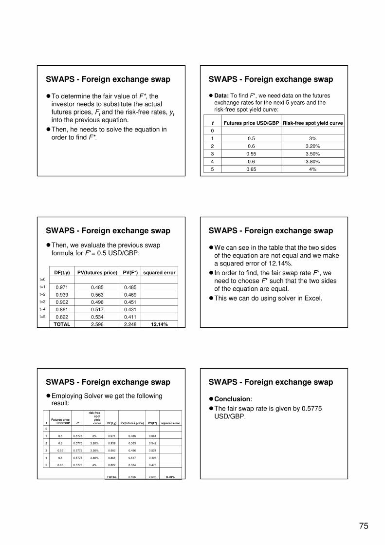
75
SWAPS - Foreign exchange swap
�To determine the fair value of F*, the investor needs to substitute the actual futures prices, Ft and the risk-free rates, yt
into the previous equation.
�Then, he needs to solve the equation in order to find F*.
SWAPS - Foreign exchange swap
� Data: To find F*, we need data on the futures exchange rates for the next 5 years and the risk-free spot yield curve:
4%0.655
3.80%0.64
3.50%0.553
3.20%0.62
3%0.51
0
Risk-free spot yield curveFutures price USD/GBPt
SWAPS - Foreign exchange swap
�Then, we evaluate the previous swap formula for F*= 0.5 USD/GBP:
12.14%2.2482.596TOTAL
0.4110.5340.822
0.4310.5170.861
0.4510.4960.902
0.4690.5630.939
0.4850.4850.971
squared errorPV(F*)PV(futures price)DF(t,y)
t=0
t=1
t=2
t=3
t=4
t=5
SWAPS - Foreign exchange swap
�We can see in the table that the two sides of the equation are not equal and we make a squared error of 12.14%.
� In order to find, the fair swap rate F*, we need to choose F* such that the two sides of the equation are equal.
�This we can do using solver in Excel.
SWAPS - Foreign exchange swap
�Employing Solver we get the following result:
0.00%2.5962.596TOTAL
0.4750.5340.8224%0.57750.655
0.4970.5170.8613.80%0.57750.64
0.5210.4960.9023.50%0.57750.553
0.5420.5630.9393.20%0.57750.62
0.5610.4850.9713%0.57750.51
0
squared errorPV(F*)PV(futures price)DF(t,y)
risk-free spot
yield curveF*
Futures price USD/GBPt
SWAPS - Foreign exchange swap
�Conclusion:
�The fair swap rate is given by 0.5775 USD/GBP.
76
INTEREST RATE SWAP
SWAPS - Interest rate swap
� Interest rate swaps (IRS) call for the exchange of a series of cash flows proportional to a fixed interest rate for a corresponding series of cash flows proportional to a floating interest rate.
�The fixed interest rate is called swap rate.
� In other words, IRS exchange a fixed interest rate payment for a floating interest rate payment.
SWAPS - Interest rate swap
Example:
�One party might exchange a variable cash flow equal to EUR 1 million times a short-term interest rate (for example EURIBOR) for EUR 1 million times a fixed interest rate of 8% for each of the next 5 years.
�Let F* = 8% denote the constant interest rate and call it swap rate.
SWAPS - Interest rate swap
�In this swap, the investor receiving the fixed interest rate obtains EUR 1 million x 8% = EUR 80.000 each of the next 5 years.
�Similarly, the investor receiving the floating interest rate obtains EUR 1 million x EURIBOR each of the next 5 years.
SWAPS - Interest rate swap
�We shall investigate whether the F* = 8% constant interest rate in this example is a correct value or not.
� In order to find the fair swap rate, F*, we exploit the analogy between a swap agreement and a sequence of futures contracts.
SWAPS - Interest rate swap
�The fair value of F* in a T-period swap is given by the next formula:
where Ft denotes the EURIBOR futures interest rate for date t and yt denotes the risk-free rate for date t.
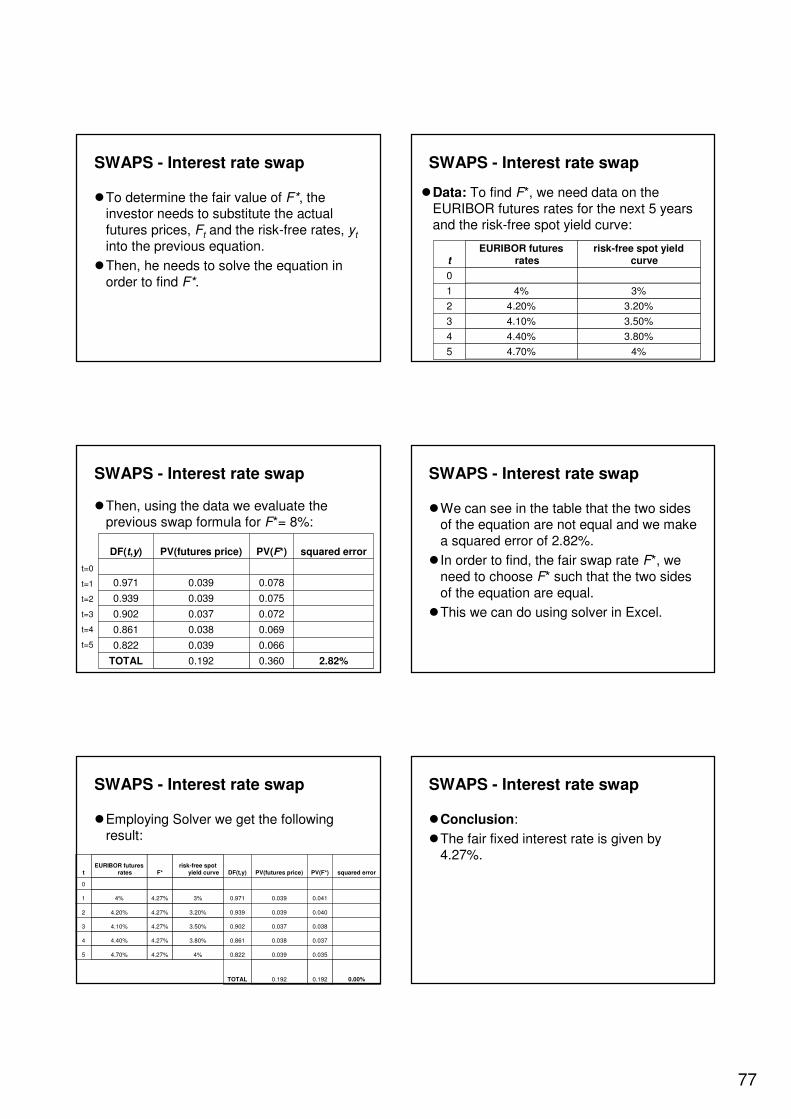
77
SWAPS - Interest rate swap
�To determine the fair value of F*, the investor needs to substitute the actual futures prices, Ft and the risk-free rates, yt
into the previous equation.
�Then, he needs to solve the equation in order to find F*.
SWAPS - Interest rate swap
�Data: To find F*, we need data on the EURIBOR futures rates for the next 5 years and the risk-free spot yield curve:
4%4.70%5
3.80%4.40%4
3.50%4.10%3
3.20%4.20%2
3%4%1
0
risk-free spot yield curve
EURIBOR futures ratest
SWAPS - Interest rate swap
�Then, using the data we evaluate the previous swap formula for F*= 8%:
2.82%0.3600.192TOTAL
0.0660.0390.822
0.0690.0380.861
0.0720.0370.902
0.0750.0390.939
0.0780.0390.971
squared errorPV(F*)PV(futures price)DF(t,y)
t=0
t=1
t=2
t=3
t=4
t=5
SWAPS - Interest rate swap
�We can see in the table that the two sides of the equation are not equal and we make a squared error of 2.82%.
� In order to find, the fair swap rate F*, we need to choose F* such that the two sides of the equation are equal.
�This we can do using solver in Excel.
SWAPS - Interest rate swap
�Employing Solver we get the following result:
0.00%0.1920.192TOTAL
0.0350.0390.8224%4.27%4.70%5
0.0370.0380.8613.80%4.27%4.40%4
0.0380.0370.9023.50%4.27%4.10%3
0.0400.0390.9393.20%4.27%4.20%2
0.0410.0390.9713%4.27%4%1
0
squared errorPV(F*)PV(futures price)DF(t,y)risk-free spot
yield curveF*EURIBOR futures
ratest
SWAPS - Interest rate swap
�Conclusion:
�The fair fixed interest rate is given by 4.27%.
78
A NOTE ONTRADITIONAL RETURN
ANDLOG-RETURN
INTRODUCTION
� There exist two alternative ways to account for return / interest:
1. Traditional return
2. Log-return or continuous return
� When we compute the future value of a cash flow using these ways of accounting returns, we have two alternative formulas.
FUTURE VALUE
�Consider the following cash flow during 1 year:
t=0 t=1
CF FV(CF)
�For this cash flow, we have two alternative formulas to compute FV:
FUTURE VALUE FORMULAS
�For traditional return:
where n denotes the number of times interest is paid during one year and rdenotes the “traditional” interest rate.
�Note that this formula assumes that we reinvest n times the interest payment.
FUTURE VALUE FORMULAS
�Continuous return:
where r denotes the continuous return.
�We will show that this formula implicitly assumes that interest is paid continuously and is reinvested continuously.
PRESENT VALUE
�Consider the following cash flow during 1 year:
t=0 t=1
PV(CF) CF
�For this cash flow, we have two alternative formulas to compute PV:

79
PRESENT VALUE FORMULAS
�The present value formulas can be obtained easily for both cases:
�Traditional return:
�Continuous return:
RELATIONSHIP BEWTEEN THE TWO RETURNS
�The two formulas can be related using the following equation:
�This equation means that if the number of interest payments and interest reinvestments during the year goes to infinity then FV(CF) and PV(CF) are equal.
RELATIONSHIP BEWTEEN THE TWO RETURNS
�Thus, we can write the next result:
and
WHY DO WE USE CONTINUOUS RETURS?
� In finance, we use continuous returns because it has some mathematical properties that make it easier to use when we do computation or modeling in finance.
�We use it because in many cases it is easier to work with continuous return than with the traditional one.
80
FINANCIAL STATEMENTS
FINANCIAL RATIOS
STURCTURE OF CLASS
1. Major financial statements
2. Ratio analysis
THE MAJOR FINANCIAL
STATEMENTS
The major financial statements
Three major financial statements are:
1. Income statement
2. Balance sheet
3. Statement of cash flows
Income statement
Income statement
�The income statement is a summary of the profitability of the firm over a period of time, such as a year.
� It represents revenues generated during the operating period, the expenses incurred during that same period, and the company’s net earning or profits, which are simply the difference between revenues and expenditures.
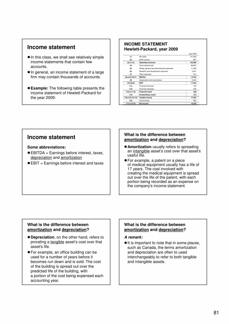
81
Income statement
� In this class, we shall see relatively simple income statements that contain few accounts.
� In general, an income statement of a large firm may contain thousands of accounts.
�Example: The following table presents the income statement of Hewlett-Packard for the year 2009:
INCOME STATEMENT Hewlett-Packard, year 2009
16,330 Net income(17)=(15-16)
993 Income taxes(16)
17,323 Taxable income(15)=(10+13+14)
(21)Extraordinary result(14)
(96)Financial result(13)=(11-12)
249 Financial expenses(12)
153 Financial revenues(11)
17,440 EBIT(10)=(8-9)
2,353 Depreciation and amortization(9)
19,793 EBITDA(8)=(3-4-5-6-7)
814 Other expenses(7)
3,591 Research and development expenses(6)
11,266 Selling, general and administrative expenses(5)
66,825 Cost of goods sold(4)
102,289 Operating revenues(3)=(1+2)
631 Other income(2)
101,658 Net sales(1)
year 2009
Income statement
Some abbreviations:
�EBITDA = Earnings before interest, taxes, depreciation and amortization
�EBIT = Earnings before interest and taxes
What is the difference between amortization and depreciation?
�Amortization usually refers to spreading an intangible asset’s cost over that asset's useful life.
�For example, a patent on a piece of medical equipment usually has a life of 17 years. The cost involved with creating the medical equipment is spread out over the life of the patent, with each portion being recorded as an expense on the company's income statement.
What is the difference between amortization and depreciation?
�Depreciation, on the other hand, refers to prorating a tangible asset’s cost over that asset's life.
�For example, an office building can be used for a number of years before it becomes run down and is sold. The cost of the building is spread out over the predicted life of the building, with a portion of the cost being expensed each accounting year.
What is the difference between amortization and depreciation?
A remark:
� It is important to note that in some places, such as Canada, the terms amortization and depreciation are often to used interchangeably to refer to both tangible and intangible assets.
82
Balance sheet
BALANCE SHEET
�The balance sheet is the list of the firm’s assets, liabilities and shareholders’equity at a moment.
Balance: ASSETS
�The first section of the balance sheet gives a listing of the assets of the firm.
�Current assets are presented first.
�Current assets are cash and other items (accounts receivable, inventories, etc.) that will be converted into cash within 1 year.
Balance: ASSETS
�Next comes the part of fixed assets.
�Within fixed assets there is a listing of long-term or fixed tangible assets, which usually consists primarily of the company’s property, plant, and equipment.
�Another part of fixed assets are intangible fixed assets such as goodwill, patents or software.
Balance: What is goodwill?
�Goodwill is an accounting term used to reflect the portion of the book value of a business entity not directly attributable to its assets and liabilities.
� It normally arises only in case of an acquisition.
� It reflects the ability of the entity to make a higher profit than would be derived from selling the tangible assets.
�Goodwill is considered an intangible asset.
Balance: ASSETS
�Example: The following table presents the assets in Hewlett-Packard’s balance sheet for dates 01/01/2009 and 12/31/2009:
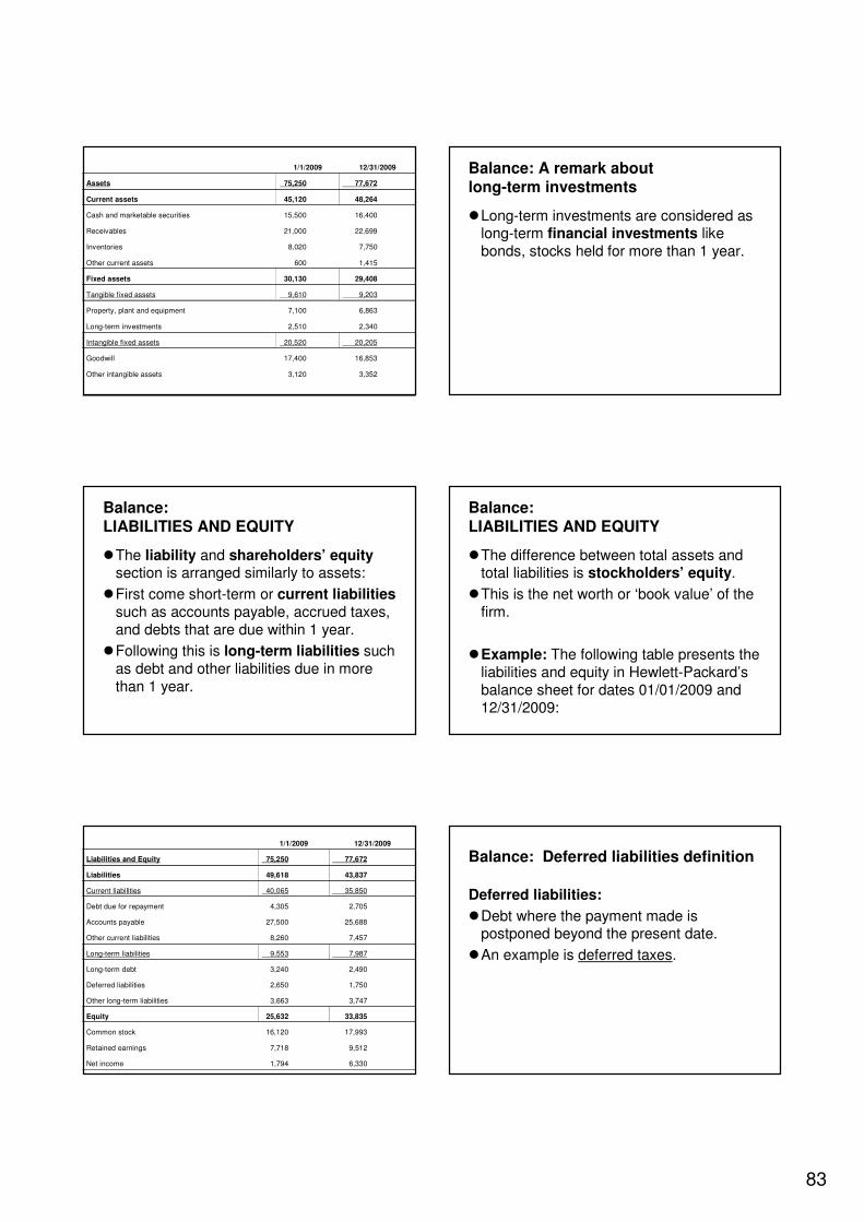
83
3,352 3,120 Other intangible assets
16,853 17,400 Goodwill
20,205 20,520 Intangible fixed assets
2,340 2,510 Long-term investments
6,863 7,100 Property, plant and equipment
9,203 9,610 Tangible fixed assets
29,408 30,130 Fixed assets
1,415 600 Other current assets
7,750 8,020 Inventories
22,699 21,000 Receivables
16,400 15,500 Cash and marketable securities
48,264 45,120 Current assets
77,672 75,250 Assets
12/31/20091/1/2009 Balance: A remark about long-term investments
�Long-term investments are considered as long-term financial investments like bonds, stocks held for more than 1 year.
Balance: LIABILITIES AND EQUITY
�The liability and shareholders’ equitysection is arranged similarly to assets:
�First come short-term or current liabilitiessuch as accounts payable, accrued taxes, and debts that are due within 1 year.
�Following this is long-term liabilities such as debt and other liabilities due in more than 1 year.
Balance: LIABILITIES AND EQUITY
�The difference between total assets and total liabilities is stockholders’ equity.
�This is the net worth or ‘book value’ of the firm.
�Example: The following table presents the liabilities and equity in Hewlett-Packard’s balance sheet for dates 01/01/2009 and 12/31/2009:
6,330 1,794 Net income
9,512 7,718 Retained earnings
17,993 16,120 Common stock
33,835 25,632 Equity
3,747 3,663 Other long-term liabilities
1,750 2,650 Deferred liabilities
2,490 3,240 Long-term debt
7,987 9,553 Long-term liabilities
7,457 8,260 Other current liabilities
25,688 27,500 Accounts payable
2,705 4,305 Debt due for repayment
35,850 40,065 Current liabilities
43,837 49,618 Liabilities
77,672 75,250 Liabilities and Equity
12/31/20091/1/2009
Balance: Deferred liabilities definition
Deferred liabilities:
�Debt where the payment made is postponed beyond the present date.
�An example is deferred taxes.

84
A remark about retained earnings and net income
�Retained earnings or reserves accumulate the net incomes of past years:
�Retained earnings(t) =
Retained earnings(t-1) + Net income(t-1)
BALANCE SHEET VERSUS INCOME STATEMENT
�While income statement provides a measure of profitability over time, the balance sheet provides a “snapshot” of the financial condition of the firm at a particular moment.
�For example, we have HP’s income statement for year 2006 and balance sheets from dates 01/01/2009 and 12/31/2009.
Statement of Cash Flows
STATEMENT OF CASH FLOWS
�The income statement and balance sheets are based on accrual methods of accounting, which means that revenues and expenses are recognized at the time of a sale even if no cash has been exchanged.
� In contrast, the statement of cash flows tracks the cash implications of transactions.
STATEMENT OF CASH FLOWS
�For example, if goods are sold now, with payment due in 60 days, the income statement will treat the revenue as generated when the sale occurs, and the balance sheet will be immediately augmented by accounts receivable, but the statement of cash flows will not showan increase in available cash until the bill is paid.
STATEMENT OF CASH FLOWS
�The statement of cash flows provides evidence on the well-being of a firm.
� If a company cannot pay its dividends and maintain the productivity of its capital stock out of cash from operations, this is a serious warning that the firm cannot maintain the dividend payout at its current level in the long run.
�The statement of cash flows will reveal this developing problem.
85
STATEMENT OF CASH FLOWS
�Another use of the statement of cash flows is in company valuation.
� In the discounted cash flow valuationtechnique, the researcher gives and estimation of future cash flows available for stockholders and creditors.
�Then, these cash flow forecasts are discounted at appropriate interest rates in order to determine the company’s present value.
STATEMENT OF CASH FLOWS
� In this class, we shall study the construction of statements of cash flows that can be used for company valuation purposes.
�We remark that the accounting law of every country defines the components and the structure of the statement of cash flows.
STATEMENT OF CASH FLOWS
�Although there is a international convergence of national accounting laws, the financial statements are different among countries and more importantly they are created not only for valuation purposes.
STATEMENT OF CASH FLOWS
� In order to get the cash flow statement for a given period (for example year 2009), one needs the following three accounting documents:
� Income statement of the period (year 2009)
�Balance sheet of the first day of the period (date 01/01/2009)
�Balance sheet of the last day of the period (date 12/31/2009)
STATEMENT OF CASH FLOWS
�The reason why we need these three documents is that the values presented in the income statement are flow typevalues that can included directly in the statement of cash flows.
�However, the values in the balance are snapshots taken on specific dates (i.e., stock type values).
STATEMENT OF CASH FLOWS
� In order, to get flow type valuespresented in the cash flow statementfrom the balance sheet one needs the compute the difference between the values of last and the first days of the period.

86
STATEMENT OF CASH FLOWS
�The general structure of the cash flow statement is presented in the next table:
FCFE = Free cash flow to equity(1+2+3+4)
Cash flow from financing activities(4)
FCFF = Free cash flow to firm(1+2+3)
Extraordinary cash flow(3)
Cash flows from investments(2)
Cash provided by operations(1)
(1) Cash provided by operations
�This is the cash flow directly coming from the firm’s operations.
�For example, in the case of Volkswagen car manufacturer company, the cash provided by operations is the cash flow related to car production, salary payments, and the sale of Volkswagen Polo cars.
�This cash flow under normal circumstances has positive value.
(2) Cash flows from investments
�This is the cash flow related to the firm’s investments in fixed non-financial assets.
�For example, in case of Volkswagen, this is the cash flow related to purchase of machines related to car production, plants, properties, and other tangible assets.
�This cash flow under normal circumstances has negative value.
(3) Extraordinary cash flow
�This cash flow is related to extraordinary events occurred during the year.
�For example, these extraordinary events can be labor accidents, natural disasters or other events that are not directly related to the normal operations of the firm.
FCFF = Free cash flow to firm
�The sum of (1), (2) and (3) is called free cash flow to firm (FCFF).
�FCFF is an important cash flow category because its represents the cash available to:
(1) Shareholders who finance the company by purchasing equity (stocks) and
(2) Creditors who finance the firm through liabilities (short- and long-term debts).
�FCFF should be positive normally.
(4) Cash flow from financing activities
�This is the cash flow related to financial assets and liabilities and financial results of the company.
�The cash flow from financing activities reflect the changes of the value of financial assets and liabilities and the profit or loss of financial operations.
�Under normal conditions, the cash flow from financing activities is negative due to the interest payments to creditors.
87
FCFE = Free cash flow to equity
�The sum of FCFF and (4) Cash flow from financing activities is called free cash flow to equity (FCFE).
�FCFE is also an important cash flow category because is represents the cash available to:
(1) Shareholders who finance the company by purchasing equity (stocks).
�The FCFE normally should be positive.
MORE DETAILED
CASH FLOW STATEMENT
More detailed structure of the Cash flow statement
�The first row in the cash flow statement is always EBIT.
� In the second row, we subtract the tax payment to compute after-tax EBIT.
�The tax payment can be defined in various ways and as a consequence we have different cash flow statements depending on how do we compute the tax payment.
More detailed structure of the Cash flow statement
� On the following slides, two alternative cash flow statements are presented:
CF1: Cash flow where Income taxes are subtracted from EBIT
CF2: Cash flow where Tax due to operating result is subtracted from EBIT
� We do this to compute the
Net Operating Profit Less Adjusted Taxes (NOPLAT).
More detailed structure of the Cash flow statement
�The difference between these two alternatives is that CF1 are CF2 are two alternatives to compute tax.
� In CF1, all the income tax presented in the income statement is subtracted from EBIT.
� In CF2, only a proportion of the income tax is subtracted from EBIT. This portion is the tax that corresponds to the operating activity and it is called ‘Tax due to operating result’.
More detailed structure of the Cash flow statement
�The CF2 can been seen as a better cash flow because in CF1 we not only subtract the tax corresponding to the operating activity from EBIT but also subtract the taxes that correspond to the extraordinary events and financial operations that have nothing to do with the basic operations of the firm.
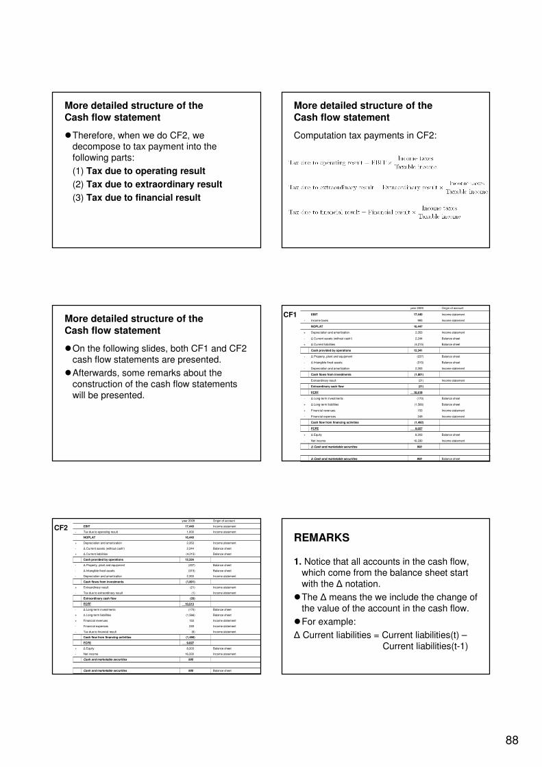
88
More detailed structure of the Cash flow statement
�Therefore, when we do CF2, we decompose to tax payment into the following parts:
(1) Tax due to operating result
(2) Tax due to extraordinary result
(3) Tax due to financial result
More detailed structure of the Cash flow statement
Computation tax payments in CF2:
More detailed structure of the Cash flow statement
�On the following slides, both CF1 and CF2 cash flow statements are presented.
�Afterwards, some remarks about the construction of the cash flow statements will be presented.
CF1
Balance sheet900 ∆ Cash and marketable securities
900 ∆ Cash and marketable securities
Income statement16,330 Net income-
Balance sheet8,203 ∆ Equity+
9,027 FCFE
(1,492)Cash flow from financing activities
Income statement249 Financial expenses-
Income statement153 Financial revenues+
Balance sheet(1,566)∆ Long-term liabilities+
Balance sheet(170)∆ Long-term investments-
10,519 FCFF
(21)Extraordinary cash flow
Income statement(21)Extraordinary result
(1,801)Cash flows from investments
Income statement2,353 Depreciation and amortization-
Balance sheet(315)∆ Intangible fixed assets-
Balance sheet(237)∆ Property, plant and equipment-
12,341 Cash provided by operations
Balance sheet(4,215)∆ Current liabilities+
Balance sheet2,244 ∆ Current assets (without cash!)-
Income statement2,353 Depreciation and amortization+
16,447 NOPLAT
Income statement993 Income taxes-
Income statement17,440 EBIT
Origin of accountyear 2009
CF2
Balance sheet900 Cash and marketable securities
900 Cash and marketable securities
Income statement16,330 Net income-
Balance sheet8,203 ∆ Equity+
9,027 FCFE
(1,486)Cash flow from financing activities
Income statement(6)Tax due to financial result-
Income statement249 Financial expenses-
Income statement153 Financial revenues+
Balance sheet(1,566)∆ Long-term liabilities+
Balance sheet(170)∆ Long-term investments-
10,513 FCFF
(20)Extraordinary cash flow
Income statement(1)Tax due to extraordinary result-
Income statement(21)Extraordinary result+
(1,801)Cash flows from investments
Income statement2,353 Depreciation and amortization-
Balance sheet(315)∆ Intangible fixed assets-
Balance sheet(237)∆ Property, plant and equipment-
12,334 Cash provided by operations
Balance sheet(4,215)∆ Current liabilities+
Balance sheet2,244 ∆ Current assets (without cash!)-
Income statement2,353 Depreciation and amortization+
16,440 NOPLAT
Income statement1,000 Tax due to operating result-
Income statement17,440 EBIT
Origin of accountyear 2009
REMARKS
1. Notice that all accounts in the cash flow, which come from the balance sheet start with the ∆ notation.
�The ∆ means the we include the change of the value of the account in the cash flow.
�For example:
∆ Current liabilities = Current liabilities(t) –Current liabilities(t-1)

89
REMARKS
2. Notice that when we compute ∆ Current assets, we do not take into account the Cash and marketable securities account from the balance sheet.
� This means that
∆ Current assets = ∆ Receivables +
∆ Inventories +
∆ Other current assets
� This is because ∆ Cash and marketable securities are presented in the last row of the cash flow table.
REMARKS
3. Related to remark 2, notice that the last two rows of the cash flow statement are ∆ Cash and marketable securities two times.
� The first row is a result of the previous rows of the table (see the computation in the first column).
� The second row directly comes from the balance sheet by ∆ Cash and marketable securities = Cash and marketable securities(t) - Cash and marketable securities(t-1).
� These two rows provide a verification of the cash flow calculation. If everything has been done well, these two rows should be equal.
REMARKS
4. Notice that the cost of depreciation and amortization is removed from cash provided by operations and included in cash flows from investments.
�This is due to the fact that depreciation is a cost related to the firm’s investments in fixed assets and not to its operations.
REMARKS
5. Notice that an increase in the value of any the assets, i.e.
∆ Asset = Asset(t) - Asset(t-1) > 0
always has negative impact on the cash flow. (See the first column of the cash flow tables for this.)
�This is because more assets mean more investments of the firms.
REMARKS
6. Notice that an increase in the value of any the liabilities or equity, i.e.
∆ Liability = Liability(t) - Liability(t-1) > 0
or
∆ Equity = Equity(t) - Equity(t-1) > 0
always has positive impact on the cash flow. (See the first column of the cash flow tables for this.)
�This is because more equity/liability means more financing of the firm.
REMARKS
7. Notice that revenues have positive while costs have negative impact on the firm’s cash flow. (See the first column of the cash flow tables for this.)
90
RATIO ANALYSIS
INTRODUCTION
�The major financial statements give an important financial and economic information of a firm’s situation.
� However, these documents contain a large amount of information that is difficult to overview.
�Therefore, in the practice analysts and company managers use several financial ratios to summarize the main accounting documents of the company.
INTRODUCTION
� These financial ratios are typically used in order to compare
1. Different firms at a given point of time. (For example, compare the profitability of two competitor firms in 2009 using a profitability ratio.)
2. Different years of the same firm. (For example, to study the evolution of the profitability of Hewlett-Packard during 2000-2009.)
INTRODUCTION
Remark:
�When the following financial ratios include one item from the income statement, which covers a period of time, and another from the balance sheet, which is a “snapshot” at a particular time, the practice is to take the average of the beginning and the end-of-year balance sheet figures.
INTRODUCTION
� We shall classify the financial ratios in the next groups:
1. Leverage ratios
2. Asset utilization ratios
3. Liquidity ratios
4. Profitability ratios
5. Market price ratios
LEVERAGE RATIOS

91
LEVERAGE RATIOS
� The following ratios will be presented:
1. Interest burden
2. Interest coverage
3. Leverage
4. Compound leverage factor
1. Interest burden
� We shall explain this ratio later.
2. Interest coverage
� A high coverage ratio indicates that the likelihood of bankruptcy is low because annual earnings are significantly greater than annual interest obligations.
� It is widely used by both lenders and borrowers in determining the firm’s debt capacity and is a major determinant of the firm’s bond rating.
3. Leverage
� We shall explain this ratio later.
4. Compound leverage factor
� We shall explain this ratio later.
ASSET UTILIZATION
RATIOS

92
ASSET UTILIZATION RATIOS
� The following ratios will be presented:
1. Total asset turnover
2. Fixed asset turnover
3. Inventory turnover
4. Days receivables
1. Total asset turnover
� This ratio measures sales per EUR of the firm’s money tied up in assets.
2. Fixed asset turnover
� This ratio measures sales per EUR of the firm’s money tied up in fixed assets.
3. Inventory turnover
� The numerator of this ratio is the cost of goods sold instead of sales revenue because inventory is valued at cost.
� This ratio measures the speed with which inventory is turned over.
4. Days receivables
� This ratio is also called average collection period.
� It is the number of days’ worth of sales tied up in accounts receivable.
� An alternative interpretation of this ratio:
� It is the average lag between the date of sale and the date payment is received.
LIQUIDITY RATIOS
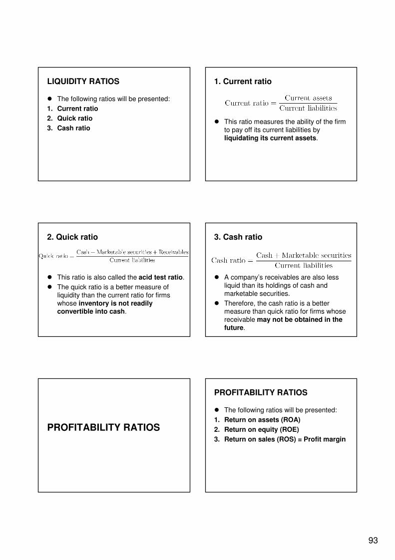
93
LIQUIDITY RATIOS
� The following ratios will be presented:
1. Current ratio
2. Quick ratio
3. Cash ratio
1. Current ratio
� This ratio measures the ability of the firm to pay off its current liabilities by liquidating its current assets.
2. Quick ratio
� This ratio is also called the acid test ratio.
� The quick ratio is a better measure of liquidity than the current ratio for firms whose inventory is not readily convertible into cash.
3. Cash ratio
� A company’s receivables are also less liquid than its holdings of cash and marketable securities.
� Therefore, the cash ratio is a better measure than quick ratio for firms whose receivable may not be obtained in the future.
PROFITABILITY RATIOS
PROFITABILITY RATIOS
� The following ratios will be presented:
1. Return on assets (ROA)
2. Return on equity (ROE)
3. Return on sales (ROS) = Profit margin
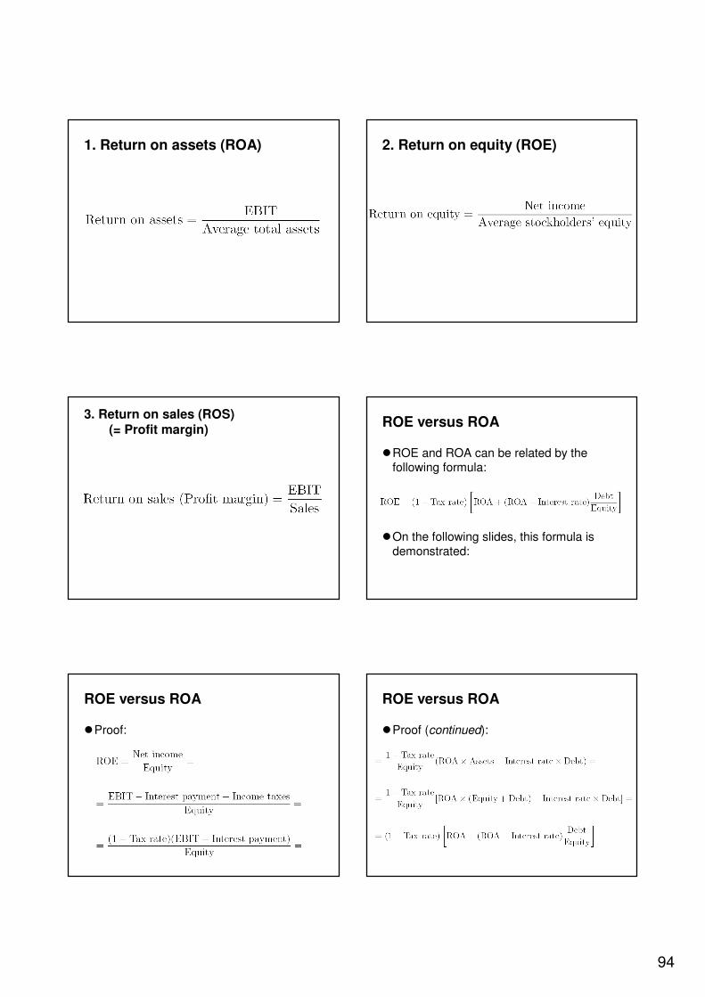
94
1. Return on assets (ROA) 2. Return on equity (ROE)
3. Return on sales (ROS) (= Profit margin)
ROE versus ROA
�ROE and ROA can be related by the following formula:
�On the following slides, this formula is demonstrated:
ROE versus ROA
�Proof:
ROE versus ROA
�Proof (continued):
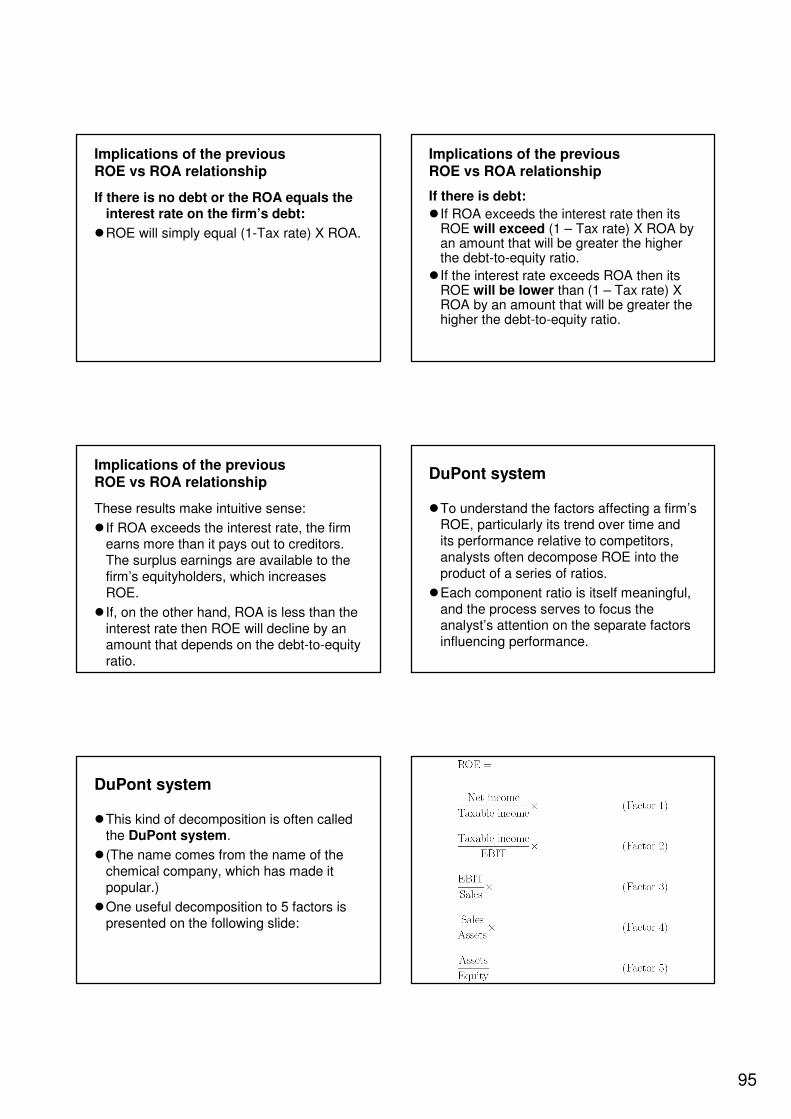
95
Implications of the previous ROE vs ROA relationship
If there is no debt or the ROA equals the interest rate on the firm’s debt:
�ROE will simply equal (1-Tax rate) X ROA.
Implications of the previous ROE vs ROA relationship
If there is debt:
� If ROA exceeds the interest rate then its ROE will exceed (1 – Tax rate) X ROA by an amount that will be greater the higher the debt-to-equity ratio.
� If the interest rate exceeds ROA then its ROE will be lower than (1 – Tax rate) X ROA by an amount that will be greater the higher the debt-to-equity ratio.
Implications of the previous ROE vs ROA relationship
These results make intuitive sense:
� If ROA exceeds the interest rate, the firm earns more than it pays out to creditors. The surplus earnings are available to the firm’s equityholders, which increases ROE.
� If, on the other hand, ROA is less than the interest rate then ROE will decline by an amount that depends on the debt-to-equity ratio.
DuPont system
�To understand the factors affecting a firm’s ROE, particularly its trend over time and its performance relative to competitors, analysts often decompose ROE into the product of a series of ratios.
�Each component ratio is itself meaningful, and the process serves to focus the analyst’s attention on the separate factors influencing performance.
DuPont system
�This kind of decomposition is often called the DuPont system.
� (The name comes from the name of the chemical company, which has made it popular.)
�One useful decomposition to 5 factors is presented on the following slide:
96
Factor 1
�Factor 1 is called the tax burden ratio.
� Its value reflects both the government’s tax code and the policies pursued by the firm in trying to minimize its tax burden.
Factor 2
�Factor 2 is called interest-burden ratio.
�The firm’s pretax profits will be the greatest when there are no interest payments to be made to debtholders.
� Its highest possible value is 1.
Factor 3
�Factor 3 is known as the firm’s operating profit margin or return on sales (ROS).
Factor 4
�Factor 4, the ratio of sales to total assets, is known as total asset turnover (ATO).
� It indicates the efficiency of the firm’s use of assets in the sense that it measures the annual sales generated by each EUR of assets.
Factor 5
�Factor 5 is called the leverage ratio.
� It is a ‘direct’ measure of the firm’s financial leverage.
�However, in the previous discussion about the relationship between ROE and ROA, we have seen that leverage helps boost ROE only if ROA is greater than the interest rate.
Factor 5
�How is this ‘indirect’ fact reflected in the DuPont system?
�To measure the full impact of leverage the analyst must take the product of the interest burden and leverage ratios (i.e., Factors 2 and 5).
�This product is called compound leverage factor:

97
DuPont system
�We can summarize the DuPont system decomposition of ROE using the previous ratio definitions as follows:
DuPont system
�An alternative decomposition can be obtained by considering the facts that:
ROA = Profit margin X Total asset turnover = Factor 3 X Factor 4
and
Compound leverage factor =
Interest burden X Leverage =
Factor 2 X Factor 5
DuPont system
�Substituting these into the previous ROE decomposition, we get the following alternative of the ROE decomposition:
ROE =
Tax burden X
ROA X
Compound leverage factor
MARKET PRICE RATIOS
MARKET PRICE RATIOS
� The following ratios will be presented:
1. Market-to-book (P/B)
2. Price-earnings ratio (P/E)
3. Earnings yield

98
1. Market-to-book (P/B)
�The market-book-value ratio (P/B) equals the market price of a share of the firm’s common stock divided by its book value.
�Remark: Book value is shareholders’equity in the Balance sheet.
1. Market-to-book (P/B)
�Analysts sometimes consider the stock of a firm with a low P/B value to be a “safer”investment, seeing the book value as the “floor” supporting the market price.
1. Market-to-book (P/B)
�Analysts presumably view book value as the level below which market price will not fall because the firm always has the option to liquidate, or sell, its assets for their book value.
�However, this view is questionable.
�Nevertheless, low P/B ratio is seen by some as providing a “margin of safety,”and some analysts will screen out or reject high P/B ratio firms in their stock selection process.
1. Market-to-book (P/B)
�An alternative interpretation of the P/B ratio is as a measure of growth opportunities.
�Empirically, firms with greater growth opportunities tend to exhibit higher multiples of P/B.
2. Price-earnings ratio (P/E)
�Remark: Earnings = Net income
�While low P/E stocks allow you to pay less per EUR of current earnings, high P/E stocks may still be better bargain if its earnings are expected to grow quickly.
�Nevertheless, most analysts believe that low P/E stocks are more attractive than high P/E stocks.
3. Earnings yield (E/P)
�Remark: Earnings = Net income

99
Relationship among ROE, P/B and P/E ratios
�We have the following relationship among ROE, P/B and P/E:
Relationship among ROE, P/B and E/P ratios
�Rearranging the previous equation we get that earnings yield can be expressed by ROE divided by the market-book-value ratio:
�Thus, a company with high ROE can have relatively low earnings yield because its P/B ratio is high.

100
COMPANY VALUATION DISCOUNTED CASH FLOW
(DCF) AND OTHER METHODS
INTRODUCTION
�The objective of this class is to present some commonly applied techniques of firm valuation.
�After the introduction, we present four valuation methods:
INTRODUCTION
1. DCF valuation
2. Economic value added (EVA) model
3. Relative valuation – multiples
4. Contingent claim valuation
�We will talk more about the DCF method.
�Valuation methods will be presented in a general setup. Therefore, they can be applied for several enterprises in many industries.
INTRODUCTION - What do we value?
�See the next simplified balance sheet:
Equity
Liabilities (Debt)
Assets
INTRODUCTION - What do we value?
� In the balance sheet, the total value of assets is equal to the sum of equity and liabilities.
�Therefore, we may value either
(1) Equity or
(2) Assets = Equity + Debt
INTRODUCTION - What do we value?
�The stockholders of the firm are interested in maximizing the value of the equity.
� In other words, investors who buy the company’s stocks on the financial market are interested in the value of equity.
101
INTRODUCTION - What do we value?
�The creditors, for example banks, who provide external financing to the company are interested in both the value of the debtand the total value of assets.
�For example, many credits are secured by specific assets of the firm (collateral). In this case, the bank is interested in the value of these assets.
FIRM
VALUATION
METHODS
FIRM VALUATION METHODS
� We review four approaches to firm valuation:
1. DCF valuation (“mark-to-model”)
2. Economic value added (EVA) model
3. Relative valuation – multiples (“mark-to-market”)
4. Contingent claim valuation (using option pricing models, firms are “real options”)
1. DCF valuation - STRUCTURE
a) Introduction
b) Cost of capital calculation
c) Analyze historical performance
d) Forecasting cash flow
e) Present value of free cash flow
1. DCF valuation - Introduction
1. DCF valuation - Introduction
�This method is based on computing the present value of future CFs generated by the company.
�When we use this method we need to analyze historical performance, value drivers and predict future CFs.
�This CF can be either
(1) CF to firm (FCFF) or
(2) CF to equity (FCFE).

102
1. DCF valuation - Introduction
� The estimation of CFs using the balance sheets and income statement, we have already seen in the Financial Statements section.
� In order to compute the value of firm or equity, we have to discount FCFF and FCFE, respectively.
� To do this, we need a discount rate (cost of capital), which is different for FCFF and FCFE.
1. DCF valuation - Introduction
�The DCF method can be applied easily when:
1. We value firms with currently positive CF that can be estimated with reliability for future periods.
2. A proxy for risk that can be used to obtain discount rates is available.
1. DCF valuation - Introduction
� The further we get from this idealized setting, the more difficult DCF valuation becomes.
� Some examples when DCF valuation may be problematic:
1. DCF valuation - Introduction
(a) Firms in trouble:
�A distressed firm generally has negative earnings and CFs currently and expects to lose money for some time in the future.
�For these firms estimating future CFs is difficult to do, since there is a strong probability of bankruptcy.
�For firms which are expected to fail, DCF valuation does not work very well since it looks at firms as providing positive CFs.
1. DCF valuation - Introduction
(b) Cyclical firms:
�The earnings and CFs of cyclical firms tend to follow the economy – rising during economic booms and falling during recessions.
� If DCF valuation is used for these firms, expected future CFs are usually smoothed out, unless the analyst undertakes the task of predicting the time and duration of economic recessions and recoveries.
1. DCF valuation - Introduction
(c) Firms with unutilized assets:
�DCF valuation reflects the value of all assets that produce CFs.
� If a firm has assets that are unutilized (i.e., do not produce any CFs), the value of these assets will not be reflected in DCF valuation.
�Nevertheless, the value of these assets can be obtained externally and then added to the value obtained by the DCF method.

103
1. DCF valuation - Introduction
(d) Firms with patents or product options:
�Firms often have unutilized patents or product options that do not produce any current CFs and are not expected to produce CFs in the near future, but nevertheless are valuable.
� If this is the case, the DCF value will understate the true value of the firm.
�Again we can overcome this problem by valuing externally then adding to the DCF.
1. DCF valuation - Introduction
(e) Firms in the process of restructuring:
�Firms in the process of restructuring often sell some of their assets, acquire other assets, and change their capital structure and dividend policy. Some of them also change their ownership structure.
�Each of these changes makes the estimation of future CFs difficult.
�However, if future CFs and discount rates reflect the effects of these changes, DCF may be useful.
1. DCF valuation - Introduction
(f) Firms involved in acquisitions:
� There are at least two specific issues to be take into account when using DCF method to value target firms:
1. Is there synergy in the merger and its value can be estimated?
2. (Especially in hostile takeovers.) What is the effect of changing management on CFs and discount rates?
1. DCF valuation - Introduction
(g) Private firms:
�The biggest problem of using DCF method to value private firms is estimating the discount rates, since most risk-return models require that parameters be estimated from historical prices on the asset being analyzed. Since securities on private firms are not traded this is not possible.
�A solution is to look at the risk of comparable firms publicly traded.
1. DCF valuation – Cost of capital
1. DCF valuation – Cost of capital
� In the financial statements section, we have already seen how to get different kinds of CFs from the income statement and two consecutive balance sheets.
�However, we also need a discount factor to compute the present value of CF.
�For different types of CF different interest rates are needed for the discount factor.
104
1. DCF valuation – Cost of capital
1. The FCFE is discounted using the cost of capital of equity (also called expected return on equity), rE.
2. The FCFF is discounted using the Weighted Average Cost of Capital (WACC) after taxes.
1. DCF valuation – Cost of capital COST OF CAPITAL OF EQUITY
� The cost of capital of equity can be estimated in several ways:
1. Capital asset pricing model (CAPM)
2. Arbitrage pricing theory (APT)
3. Dividend growth model
1. DCF valuation – Cost of capital 1. CAPM
�The CAPM determines the expected return of equity as follows:
rE = rf + βE (rM – rf)
where
rf is the risk-free rate (for example the yield to maturity of Treasury bills or Treasury bonds) and
rM is the expected return of the stock market (for example the return of the market index like S&P500 or IBEX).
1. DCF valuation – Cost of capital 1. CAPM
� (rM – rf) is the market risk premium,
�βE (called “beta”) is a parameter that captures the risk associated to the return of equity of firm E, and
� rE: is the expected return of equity of firm E.
1. DCF valuation – Cost of capital 1. CAPM
� As βE is different for each company, it can be considered as a risk measure of the firm’s equity.
� βE measures how the stock market return affects the stock return of firm E.
� βE can be either positive or negative:
1. If the market index increases and βE>0 then the stock price increases.
2. If the market index increases and βE<0 then the stock price decreases.
1. DCF valuation – Cost of capital 2. APT
�Another popular model of expected stock return is the APT.
� It is formulated as follows:
rE = c + βE1 F1 +...+ βEN FN
�where Fi denotes the i-th risk factor of the stock return.
�APT can be seen as an extension of CAPM because CAPM is a one-factor model where the factor is the market risk premium.
105
1. DCF valuation – Cost of capital Estimation of CAPM and APT
�The parameters of CAPM and APT can be estimated by ordinary least squares (OLS) using the following linear regressions:
�CAPM:
rEt = rft + βE (rMt – rft) + εEt
�APT:
rEt = c + βE1 F1t +...+ βEN FNt + εEt
�where the variables are observed over t=1,...,T and εEt is the i.i.d error term with E[εEt]=0 and Var[εEt]=σ
2.
1. DCF valuation – Cost of capital 3. Dividend growth model
�This approach is based on the DCF model that can be used to value a firm in stable growth.
�For a firm, which has a stable growth rate in earnings and dividends, the present value of CFs on a share of equity can be written as follows:
1. DCF valuation – Cost of capital 3. Dividend growth model
where S0 is the price of a stock today, DIV1 are dividends per share next year, rE
is the expected yield on equity, and g is the growth rate of dividends.
�Notice that this formula is the present value of a growing perpetuity.
1. DCF valuation – Cost of capital 3. Dividend growth model
�Manipulating this formula we get:
�This formula can be used to estimate the expected return of equity.
�The formula tells us that rE equals to the sum of expected dividend yield and growth rate in dividends.
1. DCF valuation – Cost of capital 3. Dividend growth model
Advantage:
�This approach is simple.
Disadvantage:
� It is limited to steady state firms. It is sensitive to estimates to growth in dividends.
1. DCF valuation – Cost of capital COST OF CAPITAL OF FIRM
�The cost of capital of firm is the weighted average of the costs of the different components of financing.
�We shall focus of two components of financing: (1) equity and (2) debt.
�Define the WACC after taxes as follows:
106
1. DCF valuation – Cost of capital WACC after taxes
where
rD = pretax expected return of debt
rD(1-Tc) = after-tax expected return of debt
Tc = corporate tax rate
rE = expected return of equity
D = market value of debt
E = market value of equity
1. DCF valuation – Cost of capital WACC: Cost of debt
� The value of the firm’s debt equals the present value of the CF to the debt holders, discounted at a rate that reflects the riskiness of that CF.
� The discount rate should equal the current market rate on similar-risk debt with comparable terms.
� The after-tax expected return of debt,rD(1-Tc) measures the current cost to the firm of borrowing funds to finance projects.
1. DCF valuation – Cost of capital WACC: Cost of debt
�Cost of debt is determined by:
(1) The current level of interest rates
(2) The default risk of the company (Use the bond ratings of the firm. Higher ratings lead to lower interest rates.)
(3) The tax advantage associated with debt (Since interest is tax deducible, the after-tax cost of debt is a function of the tax rate. This benefit increases as the tax rate Tc
increases.)
1. DCF valuation – Cost of capitalWACC: Why market value is used?
�The cost of capital measures the cost of issuing securities and these securities are issued at market value, not at book value.
�Some say that book value is more reliable because it is more stable than market value, i.e. it is not so volatile.
�However, this is more a weakness of book value measure because the true value of firms changes as firm-specific and market-wide information is revealed.
1. DCF valuation – Cost of capital Example 1
�The annual yield to maturity of Spanish treasury bonds is 3%. The annual return of IBEX is 15%. The “beta” of the firm is 2.
�Use the CAPM to compute the expected return of equity of firm E!
1. DCF valuation – Cost of capital Example 1
�Solution:
rE = rf + β (rM – rf) =
3% + 2(15%-3%) =
3% + 2x12% =
3% + 24% =
27%

107
1. DCF valuation – Cost of capital Example 2
Using the expected return of equity obtained in example 1, compute the WACC after taxes knowing that:
�The yield of the debt is 6%.
�The corporate tax rate is 15%.
�The market value of debt of firm E is 10 Millions EUR.
�The stock market capitalization of firm E is 20 Millions EUR.
1. DCF valuation – Cost of capital Example 2
�Solution:
WACC after taxes =
rD(1-Tc)D/(D+E) + rEE/(D+E) =
6%(1-15%)10m/(10m+20m) +
27%x20m/(10m+20m) =
6%x85%x10m/30m +
27%x20m/30m =
1,7% + 18% =
19,7%
1. DCF valuation –Analyze historical performance
1. DCF valuation - Analyze historical performance
�The first step in valuing a business is analyzing its historical performance.
�A sound understanding of the company’s past cash flows provides an essential perspective for developing and evaluating forecasts of future cash flows.
�Historical performance analysis should focus on the key drivers of cash flow. (See the value drivers section later in the EVA section.)
1. DCF valuation - Analyze historical performance
�The historical analysis should be developed in an integrated way.
�For example, in addition to return in invested capital (ROIC) itself, the key components of ROIC should be analyzed.
�The historical analysis should not be just a collection of ratios. Financial ratios that largely duplicate the core ratios or ratios that do not help to explain the core drivers of cash flow should not be used.
1. DCF valuation - Analyze historical performance
�Once we have calculated the determinants of historical cash flow, we analyze the results looking for trends and making comparisons with other companies in the same industry.
�We can assemble this analysis into an integrated perspective, which combines the financial analysis with an analysis of the industry structure and qualitative assessment of the company’s strengths and vulnerabilities.

108
1. DCF valuation - Analyze historical performance
�Developing this integrate perspective is not a mechanical process, so it is difficult to generalize.
�While it is impossible to provide a comprehensive checklist for understanding a company’s historical performance, here are some things to keep in mind:
1. DCF valuation - Analyze historical performance
(1) Look back in time as far as possible (at least ten years). This will help to understand whether the company and the industry tend to revert to some normal level of performance over time and whether short term trends are likely to be permanent breaks from the past.
1. DCF valuation - Analyze historical performance
(2) Go as deep into the value drivers as you can, getting as close to operational performance measures as possible.
(3) If there are any radical changes in performance, identify the source of the change and determine whether it is real or perhaps just an accounting effect and whether any change is likely to be sustained.
1. DCF valuation - Analyze historical performance
�The final step in the historical analysis is understanding the financial health of the company from a credit perspective.
�Here we are not concerned with value creation itself, but with how the company has been financing its value creation.
�To explain the company’s financial health from a credit perspective we need to answer to the following questions:
1. DCF valuation - Analyze historical performance
� Is the company generating or consuming cash?
�How much debt does the company employ relative to equity?
�What margin of safety does the company have with respect to its debt financing?
1. DCF valuation – Forecasting
109
1. DCF valuation – Forecasting
�Once we have analyzed the company’s historical performance, we can move on to forecasting its future performance.
�While we cannot provide specific forecasting rules, we can consider the following basic steps when developing forecasts:
1. DCF valuation – Forecasting
� (1) Evaluate the company’s strategic position, considering both the industry characteristics as well as the company’s competitive advantages or disadvantages.
�This will help to assess the company’s growth potential and its ability to earn returns above its cost of capital.
1. DCF valuation – Forecasting
� (2) Develop performance scenarios for the company and its industry that describe qualitatively how the company’s performance will evolve and the critical events that are likely to impact that performance.
1. DCF valuation – Forecasting
� (3) Forecast individual income-statement and balance-sheet line items based on the scenarios.
�These line items will then be aggregated to forecast free cash flow.
� (4) Check the overall forecast for reasonableness, particularly the key determinants of value (i.e., value drivers).
1. DCF valuation – Forecasting
�On the following slides some details of the previous points are presented.
1. DCF valuation – Forecasting
(1) Evaluate strategic position
110
1. DCF valuation – Forecasting Evaluate strategic position
� In order to earn returns on capital in excess of the opportunity cost of capital, companies must develop and exploit a competitive advantage.
�Without a competitive advantage, competition would force all the companies in the industry to earn only their cost of capital.
1. DCF valuation – Forecasting Evaluate strategic position
�Therefore, to develop a point of view about a company’s ability to earn an attractive profit on capital invested, we must identify the company’s potential for generating competitive advantage, given the nature of the industry in which it competes and its own assets and capabilities.
1. DCF valuation – Forecasting Evaluate strategic position
�Competitive advantages that influence positively the value of the company can be categorized into three types:
� (1) Providing superior value to the customer through a combination of price and product attributes that cannot be replicated by competitors.
�These attributes can be tangible (“the fastest computer”) or intangible (“a strong relationship between salesperson and buyer”).
1. DCF valuation – Forecasting Evaluate strategic position
� (2) Achieving lower cost than competitors.
� (3) Utilizing capital more productively than competitors.
�A competitive advantage must ultimately be expressed in terms of one or more of these characteristics.
�Describing competitive advantages this way also helps to begin to shape the financial forecast.
1. DCF valuation – Forecasting Evaluate strategic position
�Two techniques for identifying competitive advantages are:
� (1) Customer segmentation analysis and
� (2) Industry structure analysis
�On the following slides we review these techniques.
1. DCF valuation – Forecasting Customer segmentation analysis
�The purpose of customer segmentation analysis is to help estimate potential market share by explicitly identifying why customers will choose one company’s products over others.
� It also tells us how difficult it will be for a competitor to differentiate itself and helps to identify how profitable each type of customer is likely to be.

111
1. DCF valuation – Forecasting Customer segmentation analysis
�Customer segmentation analysis segments customers from two perspectives (1) the customer and (2) the producer.
1. DCF valuation – Forecasting Customer segmentation analysis
�From the customer perspective, product attributes have different importance to different groups of customers.
�For example, after-sale service may be more important to a small manufacturing customer than a large customer with its own in-house maintenance staff.
� In addition, different competitors may include different attributes in their product offering and deliver different benefits to customer groups.
1. DCF valuation – Forecasting Customer segmentation analysis
�A customer segment is a group of customers to whom similar product attributes provide similar benefits.
�Segmenting customers forces the analyst to understand why competitive market share may differ across customer groups and to find opportunities for differentiation to segments.
1. DCF valuation – Forecasting Customer segmentation analysis
�For example, in the overnight package delivery business, detailed billing information on each package is important to some customers, while others are content with summary data.
�Some customers want to be able to know instantaneously where a package is at any point in time, while other customers can wait for the information.
1. DCF valuation – Forecasting Customer segmentation analysis
�From the producer perspective, different customers have different costs to serve.
�For example, in the salt industry, distance to the customer has a major impact on the cost on the cost to serve because of salt’s low value-to-weight characteristics.
�Accordingly, some customers may be simply too far away too serve if competitors are much closer.
1. DCF valuation – Forecasting Customer segmentation analysis
�By segmenting customers according to both the customer and producer attributes, and then comparing a company’s ability to satisfy those customers relative to competitors, we can begin to identify current or potential competitive advantages.
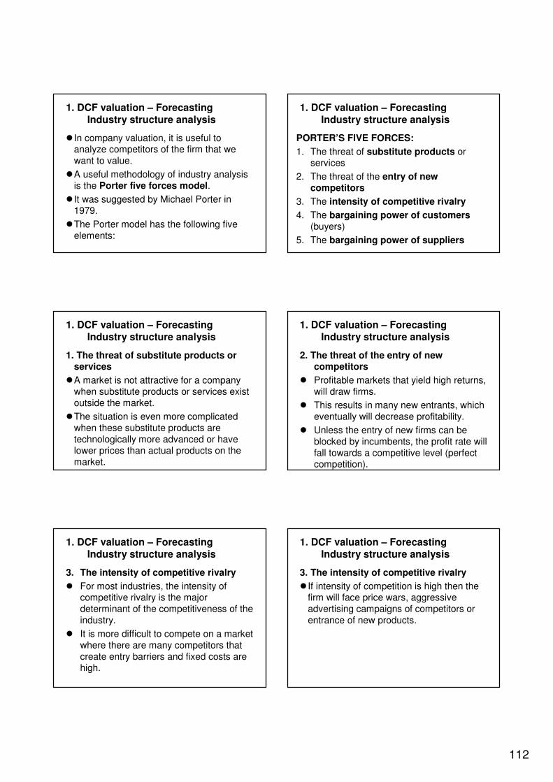
112
1. DCF valuation – Forecasting Industry structure analysis
� In company valuation, it is useful to analyze competitors of the firm that we want to value.
�A useful methodology of industry analysis is the Porter five forces model.
� It was suggested by Michael Porter in 1979.
�The Porter model has the following five elements:
1. DCF valuation – Forecasting Industry structure analysis
PORTER’S FIVE FORCES:
1. The threat of substitute products or services
2. The threat of the entry of new competitors
3. The intensity of competitive rivalry
4. The bargaining power of customers(buyers)
5. The bargaining power of suppliers
1. DCF valuation – Forecasting Industry structure analysis
1. The threat of substitute products or services
�A market is not attractive for a company when substitute products or services exist outside the market.
�The situation is even more complicated when these substitute products are technologically more advanced or have lower prices than actual products on the market.
1. DCF valuation – Forecasting Industry structure analysis
2. The threat of the entry of new competitors
� Profitable markets that yield high returns, will draw firms.
� This results in many new entrants, which eventually will decrease profitability.
� Unless the entry of new firms can be blocked by incumbents, the profit rate will fall towards a competitive level (perfect competition).
1. DCF valuation – Forecasting Industry structure analysis
3. The intensity of competitive rivalry
� For most industries, the intensity of competitive rivalry is the major determinant of the competitiveness of the industry.
� It is more difficult to compete on a market where there are many competitors that create entry barriers and fixed costs are high.
1. DCF valuation – Forecasting Industry structure analysis
3. The intensity of competitive rivalry
� If intensity of competition is high then the firm will face price wars, aggressive advertising campaigns of competitors or entrance of new products.

113
1. DCF valuation – Forecasting Industry structure analysis
4.The bargaining power of customers (buyers)
�The bargaining power of customers is also described as the market of outputs: the ability of customers to put the firm under pressure, which also affects the customer's sensitivity to price changes.
�Well-organized buyers can ask for price reductions, higher quality of products and services decreasing the company’s profit margin.
1. DCF valuation – Forecasting Industry structure analysis
5.The bargaining power of suppliers
�The bargaining power of suppliers is also described as the market of inputs.
�Suppliers of raw materials, components, labor, and services (such as expertise) to the firm can be a source of power over the firm, when there are few substitutes.
�Suppliers may refuse to work with the firm, or, e.g., charge excessively high prices for unique resources.
1. DCF valuation – Forecasting Industry structure analysis
Summary:
�A detailed analysis of these five forces can give the analyst a complex picture of the firm’s industry.
� It can help to identify the value drivers that affect future CFs and cost of capital of the firm.
�Therefore, it can help in CF prediction and present value calculation as well.
1. DCF valuation – Forecasting
(2) Develop performance scenarios
1. DCF valuation – Forecasting Develop performance scenarios
�Once we have developed a point of view about the company’s ability to achieve and sustain a competitive advantage, the next step is to develop performance scenarios.
�By using scenarios we acknowledge that forecasting financial performance is at best an educated guess.
�The best we can do is narrow down the range of likely future performance.
1. DCF valuation – Forecasting Develop performance scenarios
�Example: Consider a high tech company that is developing a new product.
� If the company successfully develops the product, its competitive advantage will be a product that delivers superior value to customers.
�Accordingly, its growth and returns on capital are likely to be huge.
� If it fails to develop the product, it will likely go out of business.
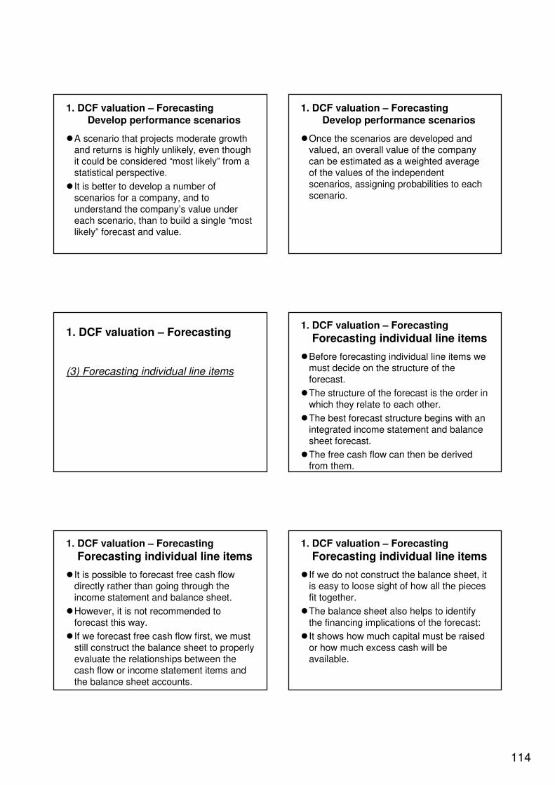
114
1. DCF valuation – Forecasting Develop performance scenarios
�A scenario that projects moderate growth and returns is highly unlikely, even though it could be considered “most likely” from a statistical perspective.
� It is better to develop a number of scenarios for a company, and to understand the company’s value under each scenario, than to build a single “most likely” forecast and value.
1. DCF valuation – Forecasting Develop performance scenarios
�Once the scenarios are developed and valued, an overall value of the company can be estimated as a weighted average of the values of the independent scenarios, assigning probabilities to each scenario.
1. DCF valuation – Forecasting
(3) Forecasting individual line items
1. DCF valuation – Forecasting
Forecasting individual line items
�Before forecasting individual line items we must decide on the structure of the forecast.
�The structure of the forecast is the order in which they relate to each other.
�The best forecast structure begins with an integrated income statement and balance sheet forecast.
�The free cash flow can then be derived from them.
1. DCF valuation – Forecasting
Forecasting individual line items
� It is possible to forecast free cash flow directly rather than going through the income statement and balance sheet.
�However, it is not recommended to forecast this way.
� If we forecast free cash flow first, we must still construct the balance sheet to properly evaluate the relationships between the cash flow or income statement items and the balance sheet accounts.
1. DCF valuation – Forecasting
Forecasting individual line items
� If we do not construct the balance sheet, it is easy to loose sight of how all the pieces fit together.
�The balance sheet also helps to identify the financing implications of the forecast:
� It shows how much capital must be raised or how much excess cash will be available.
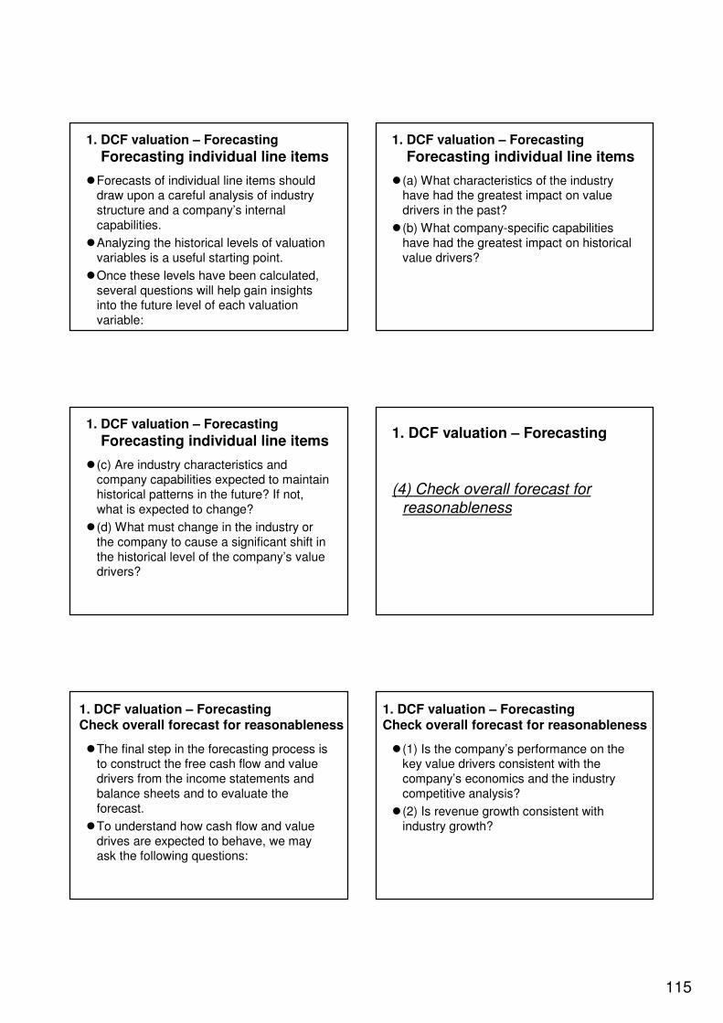
115
1. DCF valuation – Forecasting
Forecasting individual line items
�Forecasts of individual line items should draw upon a careful analysis of industry structure and a company’s internal capabilities.
�Analyzing the historical levels of valuation variables is a useful starting point.
�Once these levels have been calculated, several questions will help gain insights into the future level of each valuation variable:
1. DCF valuation – Forecasting
Forecasting individual line items
� (a) What characteristics of the industry have had the greatest impact on value drivers in the past?
� (b) What company-specific capabilities have had the greatest impact on historical value drivers?
1. DCF valuation – Forecasting
Forecasting individual line items
� (c) Are industry characteristics and company capabilities expected to maintain historical patterns in the future? If not, what is expected to change?
� (d) What must change in the industry or the company to cause a significant shift in the historical level of the company’s value drivers?
1. DCF valuation – Forecasting
(4) Check overall forecast for reasonableness
1. DCF valuation – Forecasting Check overall forecast for reasonableness
�The final step in the forecasting process is to construct the free cash flow and value drivers from the income statements and balance sheets and to evaluate the forecast.
�To understand how cash flow and value drives are expected to behave, we may ask the following questions:
1. DCF valuation – Forecasting Check overall forecast for reasonableness
� (1) Is the company’s performance on the key value drivers consistent with the company’s economics and the industry competitive analysis?
� (2) Is revenue growth consistent with industry growth?

116
� (3) If the company’s revenue is growing faster than the industry’s, which competitors are losing share? Will they retaliate?
� (4) Does the company have the resources to manage that rate of growth?
� (5) Is the return on capital consistent with the industry’s competitive structure?
� (6) If entry barriers are coming down, shouldn’t expected returns decline?
1. DCF valuation – Forecasting Check overall forecast for reasonableness
� (7) If customers are becoming more powerful, will margins decline?
� (8) Conversely, if the company’s position in the industry is becoming much stronger, should one expect increasing returns?
� (9) How will returns and growth look relative to the competition?
� (10) How will technology changes affect returns? Will they affect risk?
1. DCF valuation – Forecasting Check overall forecast for reasonableness
� (11) Can the company manage all the investment it is undertaking?
� (12) Will the company have to raise large amounts of capital? If so, can it obtain the financing? Should it be debt or equity?
� (13) If the company is generating excess cash, what options does it have for investing the cash or returning it to shareholders?
1. DCF valuation – Forecasting Check overall forecast for reasonableness
Three additional topics
1. DCF valuation – Forecasting Three additional topics of forecasts
�On the following slides we mention three additional topics related to forecasting free cash flow:
(1) Inflation,
(2) Length of the forecast, and
(3) Extraordinary items
1. DCF valuation – Forecasting Inflation
� It is recommended that financial forecasts and discount rates be estimated in nominal rather than real currency units.
�For consistency, both the free cash flow forecast and the discount rate must be based on the same expected general inflation rate.

117
1. DCF valuation – Forecasting Inflation
� Individual line items, however, could have specific inflation rates that are higher or lower that the general rate, but they should still drive off the general rate.
�We can derive the expected general inflation rate that is consistent with the discount rate from the term structure of interest rates.
�The term structure is based on yields to maturity of government bonds.
1. DCF valuation – Forecasting Inflation
�The term structure of interest rates provides a market-based estimate of expected inflation over time.
�This should be the best estimate for valuation purposes for three reasons:
� (1) Most economics’, or econometric, forecasts of inflation rarely extend beyond one or two years, far too short a period for valuation.
1. DCF valuation – Forecasting Inflation
� (2) Market-based estimates provide a broader consensus view (with investors’money at stake) than individual forecasts.
� (3) Empirical analysis suggests that market-based estimates are the least biased.
1. DCF valuation – Forecasting Inflation
�The next figure shows and example of the term structure of interest rates at different points of time in the U.S.:
Term structure of interesrest rates U.S.
0.00%
2.00%
4.00%
6.00%
8.00%
10.00%
12.00%
14.00%
16.00%
1 2 3 4 5 6 7 8 9 10 11 12 13 14 15 16 17 18 19 20 21 22 23 24 25 26 27 28 29 30
Years to maturity
Yie
ld t
o m
atu
rity
Dec-81
Jun-88
Dec-92
1. DCF valuation – Forecasting Inflation
1. DCF valuation – Forecasting Inflation
�On the previous figure we can see that in December 1981 the market expected that future inflation will be lower than near-term inflation.
�On the other hand, in June 1988 and December 1992 the market expected that future inflation will be higher than near-term inflation.
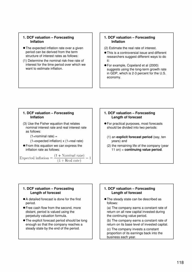
118
1. DCF valuation – Forecasting Inflation
�The expected inflation rate over a given period can be derived from the term structure of interest rates as follows:
(1) Determine the nominal risk-free rate of interest for the time period over which we want to estimate inflation.
1. DCF valuation – Forecasting Inflation
(2) Estimate the real rate of interest.
�This is a controversial issue and different researchers suggest different ways to do it:
�For example, Copeland et al (2000) suggests using the long-term growth rate in GDP, which is 2-3 percent for the U.S. economy.
1. DCF valuation – Forecasting Inflation
(3) Use the Fisher equation that relates nominal interest rate and real interest rate as follows:
(1+nominal rate) =
(1+expected inflation) x (1+real rate)
�From this equation we can express the inflation rate as follows:
1. DCF valuation – Forecasting Length of forecast
�For practical purposes, most forecasts should be divided into two periods:
(1) an explicit forecast period (say, ten years) and
(2) the remaining life of the company (year 11 on) = continuing value period.
1. DCF valuation – Forecasting Length of forecast
�A detailed forecast is done for the first period.
�Free cash flow from the second, more distant, period is valued using the perpetuity valuation formula.
�The explicit forecast period should be long enough so that the company reaches a steady state by the end of the period.
1. DCF valuation – Forecasting Length of forecast
�The steady state can be described as follows:
(a) The company earns a constant rate of return on all new capital invested during the continuing value period.
(b) The company earns a constant rate of return on its base level of invested capital.
(c) The company invests a constant proportion of its earnings back into the business each year.

119
1. DCF valuation – Forecasting Length of forecast
�The most common approach is to make the forecast period as long as you expect the company to have sustainable rates of return on new investment above the company’s cost of capital.
�Microeconomic analysis suggests that over time, competition will drive the returns in many industries to the level of the cost of capital.
1. DCF valuation – Forecasting Length of forecast
�Once the company’s returns have converged on its cost of capital, it is relatively simple to estimate the company’s continuing value.
�Therefore, forecasting until convergence simplifies the continuing value problem.
� If we use this approach, the forecast periods should be for as long as returns above the WACC are sustainable.
1. DCF valuation – Forecasting Length of forecast
�When in doubt, make a longer rather than shorter forecast.
�We would rarely use a forecast period of less than seven years.
�The forecast period should never be determined by the company’s own internal planning period.
�Just because the company forecasts out only three years does not justify using three years for valuation.
1. DCF valuation – Forecasting Length of forecast
� If a company is in a cyclical industry, it is important that your forecast capture complete cycle.
�Failure to do so may result in wildly unrealistic continuing value assumptions, because the up or down phase of the cycle may be projected to last forever.
� It is best to put long-run forecasts (averaging out cyclical effects) into the continuing value assumptions.
1. DCF valuation – Forecasting Extraordinary items
�Financial documents always contain some extraordinary events that are partly reflected in the extraordinary result of the income statement.
�The extraordinary elements of financial documents are recommended to be excluded from all financial documents before forecasting free cash flow.
1. DCF valuation –
Present value of free cash flow
120
1. DCF valuation – Present value of free cash flow
�After forecasting the free cash flow, we compute the present value of FCFE and FCFF to get the value of the firm.
�The present value of FCFE is the value ofequity.
�The present value of FCFF is the value of equity + value of debt (i.e., the value of total assets).
1. DCF valuation – Present value of free cash flow
�The FCFE values have to be discounted using the expected return on equity, rE.
�The FCFF values must be discounted using the Weighted Average Cost of Capital (WACC) after taxes.
1. DCF valuation – Present value of free cash flow
�For the first, explicit forecast period, we can use the next formulas in order to calculate the present value of free cash flows:
1. DCF valuation – Present value of free cash flow
�Computation of present value of a cash flow obtained at year t, CFt:
PV(CFt) = CFt / (1+r)t
�Present value of FCFEt:
PV(FCFEt) = FCFEt / (1+rE)t
�Present value of FCFFt:
PV(FCFFt) = FCFFt / (1+WACC)t
1. DCF valuation – Present value of free cash flow
�For the second, continuing value period we use the following formulas to value the cash flow of a growing perpetuity:
1. DCF valuation – Present value of free cash flow
�Suppose that in steady state the cash flow is a growing perpetuity:
t=0, t=1, t=2, t=3,…….
0 CF1 CF2 CF3
where the growth rate of the cash flow is g:
CFt+1 = (1+g) x CFt

121
1. DCF valuation – Present value of free cash flow
�The present value of a growing perpetuity at time t=0 is given by:
PV(growing perpetuity with rate g) =
CF1 / (r-g)
where
CF1 = cash flow at t=1
r = expected return
g = growth rate
1. DCF valuation – Present value of free cash flow
�Assuming that the continuing value period starts at year t=6, we have the next growing perpetuity:
�Therefore, the present value of the free cash flow over the continuing value period is:
PV(CF continuing value) = CF6/[(r-g)(1+r)5]
CF6 (1+g)2CF6 (1+g)CF6000000
t=8t=7t=6t=5t=4t=3t=2t=1t=0
1. DCF valuation – Present value of free cash flow
191.6158.0130.3107.588.673.1FCFE
171.6145.7123.7105.089.275.7FCFF
2014 20132012201120102009
3%g
15%rE
10%WACC
Example: Cash flow forecasts for the following 6 years (2009-2014):
Suppose that the expected returns and perpetuity growth rate are:
1. DCF valuation – Present value of free cash flow
�The FCFE and FCFF values for 2009-2013 are discounted using the following formulas:
PV(FCFEt) = FCFEt / (1+rE)t
PV(FCFFt) = FCFFt / (1+WACC)t
�The cash flow for the continuing value period is discounted as follows:
PV(continuing value) = CF6/[(r-g)(1+r)5]
1. DCF valuation – Present value of free cash flow
1148.2PV(TOTAL: FCFE)
1918.5PV(TOTAL: FCFF)
793.978.674.570.767.063.5PV(FCFE)
1522.190.584.578.973.768.8PV(FCFF)
Continuing
value20132012201120102009
In the next table, we present the present value of FCFE and FCFF:
1. DCF valuation – Present value of free cash flow
�The total present value is computed using the next formulas:
122
1. DCF valuation – Present value of free cash flow
Solution:
�The value of equity of the firm is 1148.2 EUR.
�The value of total assets is 1918.5 EUR.
2. Economic value added (EVA)
2. EVA – Structure
� In this section, first we will introduce the concept of value drivers.
�Then, we define EVA and present the firm valuation model using EVA.
�Finally, we show that the value provided with DCF coincides with EVA valuation in our setup.
2. EVA – Value drivers
�To understand the idea of valuation by EVA we need to identify the underlying economic value drivers of the business.
�Since value is based on discounted cash flow, the underlying value drivers of the business must also be the drivers of free CF.
2. EVA – Value drivers
� There are two key drivers of free CF and, as a consequence, value:
1. The net investment rate that the company invests from NOPLAT in each period to earn additional profits and
2. The return on (operating) invested capital (ROIC)
� These value drivers are consistent with common sense:
2. EVA – Value drivers
�A company that invests more (i.e., grows faster) will worth more than a company that invests less (i.e., grows slower) if they are both earning the same return on invested capital.
�Similarly, a company that earns higher profits for every dollar invested in the business will worth more than a similar company that earns less profits for every dollar of invested capital.
123
2. EVA – Value drivers
ROIC
�We shall demonstrate how investment rate and ROIC actually drive CF.
�First, some definitions are needed:
where NOPLAT = Net operating profits less adjusted taxes. (We have seen this in the Financial statements section.)
2. EVA – Value drivers
Operating invested capital
�What is operating invested capital?
�Operating invested capital =
Operating working capital +
Net property, plant and equipment +
Net other operating assets
2. EVA – Value drivers
Operating working capital
�Operating working capital =
(1) Operating current assets –
(2) Noninterest bearing current liabilities
� (1) Operating current assets = all current assets used in or necessary for the operations of the business
� (2) Noninterest bearing current liabilities = (accounts payable + accrued expenses + other noninterest bearing liabilities)
2. EVA – Value drivers
Other net operating fixed assets
�Net property, plant and equipment = The book value of the company’s property, plant and equipment related to the operations of the business net of noncurrent, noninterest bearing liabilities.
�Net other operating assets = other operating assets, net of other liabilities. Any other assets net of noninterest bearing liabilities that are related to the operations of the business.
2. EVA – Value drivers
Simplifying assumptions
�We present a simple example to show how the two value drivers impact CF and firm value.
Assumptions:
�Assume that the firm lives infinite periods.
�Assume that in the initial year NOPLAT = 100 Euros.
�Assume that net investment rate and ROICare constant.
2. EVA – Value drivers
Simple CF statement
� We will work with the following simplified FCFF statement:
NOPLAT- Net investment (∆ operating invested capital)
= FCFF
� Remark: net investment is the change of the value of operating invested capital.
� First, we compute FCFF for several periods and show that the FCFF growth rate is the product of investment rate and ROIC.
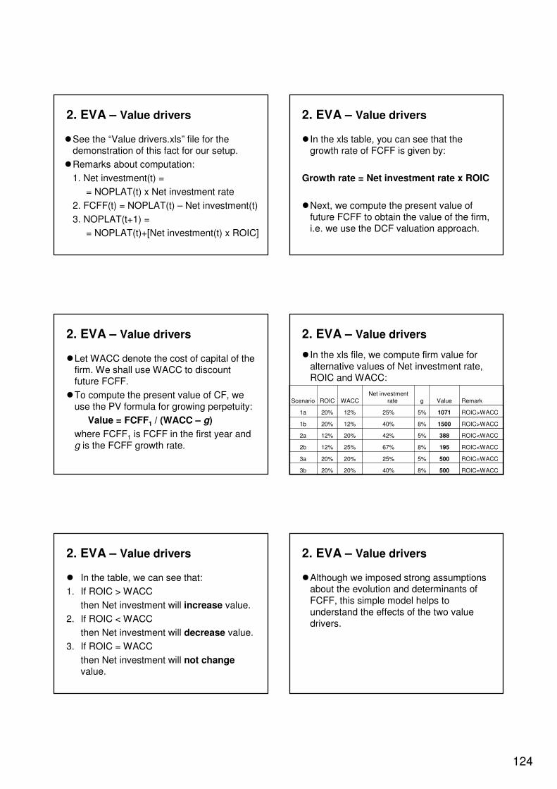
124
2. EVA – Value drivers
�See the “Value drivers.xls” file for the demonstration of this fact for our setup.
�Remarks about computation:
1. Net investment(t) =
= NOPLAT(t) x Net investment rate
2. FCFF(t) = NOPLAT(t) – Net investment(t)
3. NOPLAT(t+1) =
= NOPLAT(t)+[Net investment(t) x ROIC]
2. EVA – Value drivers
� In the xls table, you can see that the growth rate of FCFF is given by:
Growth rate = Net investment rate x ROIC
�Next, we compute the present value of future FCFF to obtain the value of the firm, i.e. we use the DCF valuation approach.
2. EVA – Value drivers
�Let WACC denote the cost of capital of the firm. We shall use WACC to discount future FCFF.
�To compute the present value of CF, we use the PV formula for growing perpetuity:
Value = FCFF1 / (WACC – g)
where FCFF1 is FCFF in the first year and g is the FCFF growth rate.
2. EVA – Value drivers
� In the xls file, we compute firm value for alternative values of Net investment rate, ROIC and WACC:
ROIC=WACC5008%40%20%20%3b
ROIC=WACC5005%25%20%20%3a
ROIC<WACC1958%67%25%12%2b
ROIC<WACC3885%42%20%12%2a
ROIC>WACC15008%40%12%20%1b
ROIC>WACC10715%25%12%20%1a
RemarkValuegNet investment
rateWACCROICScenario
2. EVA – Value drivers
� In the table, we can see that:
1. If ROIC > WACC
then Net investment will increase value.
2. If ROIC < WACC
then Net investment will decrease value.
3. If ROIC = WACC
then Net investment will not changevalue.
2. EVA – Value drivers
�Although we imposed strong assumptions about the evolution and determinants of FCFF, this simple model helps to understand the effects of the two value drivers.
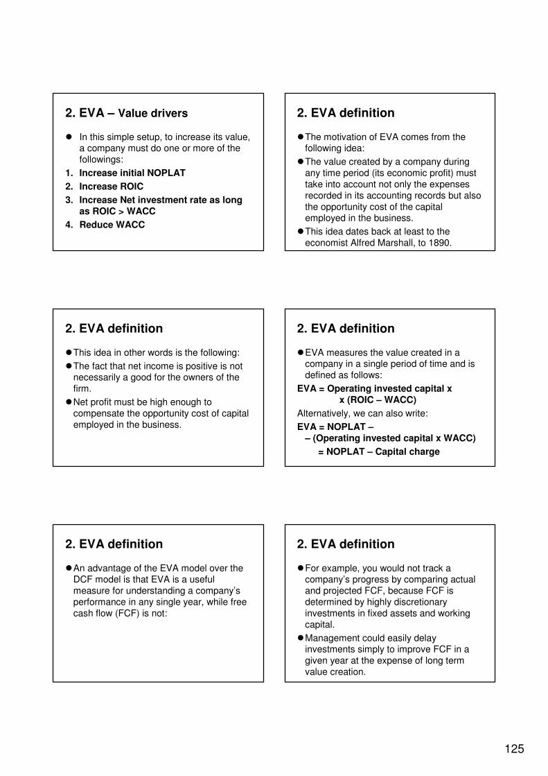
125
2. EVA – Value drivers
� In this simple setup, to increase its value, a company must do one or more of the followings:
1. Increase initial NOPLAT
2. Increase ROIC
3. Increase Net investment rate as long as ROIC > WACC
4. Reduce WACC
2. EVA definition
�The motivation of EVA comes from the following idea:
�The value created by a company during any time period (its economic profit) must take into account not only the expenses recorded in its accounting records but also the opportunity cost of the capital employed in the business.
�This idea dates back at least to the economist Alfred Marshall, to 1890.
2. EVA definition
�This idea in other words is the following:
�The fact that net income is positive is not necessarily a good for the owners of the firm.
�Net profit must be high enough to compensate the opportunity cost of capital employed in the business.
2. EVA definition
�EVA measures the value created in a company in a single period of time and is defined as follows:
EVA = Operating invested capital x x (ROIC – WACC)
Alternatively, we can also write:
EVA = NOPLAT –– (Operating invested capital x WACC)
= NOPLAT – Capital charge
2. EVA definition
�An advantage of the EVA model over the DCF model is that EVA is a useful measure for understanding a company’s performance in any single year, while free cash flow (FCF) is not:
2. EVA definition
�For example, you would not track a company’s progress by comparing actual and projected FCF, because FCF is determined by highly discretionary investments in fixed assets and working capital.
�Management could easily delay investments simply to improve FCF in a given year at the expense of long term value creation.

126
2. Valuation with EVA
�The EVA model says that the value of a company equals the amount of capital invested, plus a premium or discount equal to present value of its predicted EVA:
�Firm value =
Operating invested capital +
Present value of predicted EVA
2. Valuation with EVA
�We follow the previous simple example to show that EVA valuation gives identical result to the DCF valuation presented before.
�See the file “EVA.xls” for the exercise.
�The initial NOPLAT = 100 and we impose the same assumptions as before:
�Assumptions: ROIC, WACC and Net investment rate are constant. Firm lives for infinite periods.
2. Valuation with EVA
�Example: DCF valuation: Value = PV(FCFF)
1071.4VALUE
Growing perpetuity
5.0%5.0%5.0%5.0%CF growth rate, g
91.286.882.778.875.0FCFF
30.428.927.626.325.0Net investment
121.6115.8110.3105.0100.0NOPLAT
54321year
12%WACC
25%Net investment rate
20%ROIC
2. Valuation with EVA
�Example: EVA valuation: Value = PV(EVA) + Operating invested capital
�Remark: In the following table, operating invested capital is computed using the definition of ROIC:
�Thus, Operating invested capital = NOPLAT / ROIC.
1071.4VALUE
500.0Operating invested capital
571.4PV(EVA)
Growing perpetuity
5.0%5.0%5.0%5.0%EVA growth rate, g
48.646.344.142.040.0EVA
607.8578.8551.3525.0500.0Operating invested capital
30.428.927.626.325.0Net investment
121.6115.8110.3105.0100.0NOPLAT
54321year
12%WACC
25%Net investment rate
20%ROIC
2. Valuation with EVA2. Valuation with EVA
�To compute the present value of EVA, we use the PV formula for growing perpetuity:
Value = EVA1 / (WACC – g)
where EVA1 is EVA in the first year and gis the EVA growth rate.
� In the “EVA.xls” file, the EVA valuation for alternative values of ROIC, WACC, and Net investment rate are presented. We can see that always the same result is obtained as in the DCF valuation.

127
3. Relative valuation - multiples
3. Relative valuation - multiples
� In relative valuation, the value of an asset is derived from the pricing of comparable assets, standardized using a common variable such as earnings, CFs, book value, or revenues.
�Example: Use the industry-average price/earnings ratio to value a firm, the assumption being that the other firms in the industry are comparable to the firm being valued and that the market prices these firms correctly.
3. Relative valuation - multiples
� The following ratios are being used in relative valuation:
1. P/E = price/earnings ratio
2. Price/book value ratio
3. Price/sales ratio
4. Price/CF ratio
5. Price/dividends ratio
6. Market value/replacement value (Tobin’s Q)
3. Relative valuation - multiples
� There are two ways of using multiples:
1. Using fundamentals
2. Using comparables
3. Relative valuation – multiples1. Using fundamentals
� In this approach, we relate the multiple to fundamental variables like CFs, payout ratios and risk.
�The advantage of this approach is that it shows the relationship between multiples and firm characteristics and allows us the explore how multiples change as these characteristics change:
� (P/E)t = α + β(Fundamental variables)t + εt
3. Relative valuation – multiples2. Using comparables
�The second approach estimates multiples for a firm by looking at a comparable firm.
�The key issue in this approach is the definition of the comparable firm.
�The analyst should control for all variables that can influence the multiple.
�Controlling for these variables can be naive (industry averages) or more sophisticated (multivariate regressions):
128
3. Relative valuation – multiples2. Using comparables
(a) Industry average approach:
where i = 1,…,k are comparable firms in the sample (for example competitors).
3. Relative valuation – multiples2. Using comparables
(b) Regression approach:
�Select n variables {X1i,…,Xni} for firm i that influence the value of the multiple. Then, estimate the next regression model:
Multiplei = α + β1X1i + … + βnXni + εi
where i = 1,…,k are comparable firms in the sample (for example competitors).
3. Relative valuation – multiples2. Using comparables
(b) Regression approach:
�After estimating the parameters of the previous regression model, we compute the multiple of firm e using the next formula::
Multiplee = α + β1X1e + … + βnXne
where the parameters included were estimated by the regression model of the previous slide.
3. Relative valuation - multiples
�After estimating the multiple of firm e by approaches (a) or (b), one can compute the price of stock e for some multipliers in the following way:
(1) Pe = (P/E)e X Ee
(2) Pe = (P/BV)e X BVe
(3) Pe = (P/Sales)e X Salese
3. Relative valuation – multiplesAdvantages
� It is relatively easy to use.
�Multiples can be used to obtain estimates of value quickly, and are particularly useful when there are a large number of comparable firms being traded on the financial market and the market is, on average, pricing these firms correctly.
3. Relative valuation – multiplesDisadvantages
�Multiples are also easy to misuse and manipulate, especially when comparable firms are used.
�Given that no two firms are exactly similar in terms of risk and growth, the definition of comparable firms is a subjective one.
�A biased analyst can choose a group of comparable firms to confirm his/her biases about a firm’s value.
129
3. Relative valuation – multiplesDisadvantages
�While this potential for bias exists with DCF valuation as well, the analyst in DCF method is forced to be more explicit about the assumptions which determine the final value.
�With multiples, these assumptions are often left unstated.
3. Relative valuation – multiplesDisadvantages
�The other problem with multiples is that it builds in errors (overvaluation or undervaluation) that the market might be making in valuing these firms.
3. Relative valuation - multiples
�Example: What is the value of my book shop with monthly sales of 3000 EUR if during the last month another book shop with monthly sales of 2000 EUR has been sold for 200,000 EUR?
�Answer: We use the Price/Sales multiple of the other shop to value our firm:
�Price/Sales = 200,000/2,000
�Value = 200,000/2,000 X 3,000 = = 300.000 EUR
4. Contingent claim valuation
4. Contingent claim valuationIntroduction
�Much work has been done in the past in developing models that value options, and these option pricing models can be used to value any asset that have option-like features. (i.e., assets that pay off under certain contingencies).
�As equity can be viewed as an option, derivative pricing models like Cox-Ross-Rubinstein or Black-Scholes can be employed to price companies.
4. Contingent claim valuationIntroduction
�A limitation of the option pricing approach of firm valuation comes from the assumptions of the option pricing model.
�For example, volatility of the underlying asset is assumed to be constant, or other unrealistic assumptions build in errors in the pricing model.
�Thus, the final values obtained from these applications of option pricing models have much more estimation errors than more standard applications.

130
4. Contingent claim valuation
�On the remaining slides of this section, application of option pricing theory to equity valuation is presented.
4. Contingent claim valuationThe general framework
�The equity in a firm is a residual claim, that is, equity holders lay claim to all CFs left over after other financial claimholders (debt, preferred stock, etc.) have been satisfied.
�The principle of limited liability, however, protects equity investors in publicly traded firms if the value of the firm is less than the value of the outstanding debt, and they cannot lose more than their investment in the firm.
4. Contingent claim valuationThe general framework
�The payoff to equity investors, on liquidation, can be written as:
V – D if V > D
Payoff =
0 if V ≤ D
where V = value of the firm, D = face value of the outstanding debt and other external claims.
�Notice that a call option with spot underlying price V and strike D has the same payoff.
4. Contingent claim valuationThe general framework
�Equity thus can be viewed as a call option on the firm value, where exercising the option requires that the firm be liquidated and the face value of the debt (which corresponds to the exercise price) be paid off.
4. Contingent claim valuationThe general framework
� If the debt is a single issue of zero-coupon bonds with a fixed lifetime and the firm can be liquidated by equity investors at any time prior, the life of the equity as a call option corresponds to the life of the bonds.
4. Contingent claim valuationThe general framework
�The next figure presents the payoff of equity as a function of the value of the firm at liquidation:
131
4. Contingent claim valuationThe general framework
Face value of debt
Value of firm
Payoff on equity
4. Contingent claim valuationExample
�Assume a firm whose assets are currently valued at 100 million USD and that the standard deviation of this asset value is 40%.
�Further, assume that the face value of debt is 80 million USD. (It is a zero-coupon debt with ten years left to maturity.)
4. Contingent claim valuationExample
� (a) If the ten-year Treasury bond rate is 10%, how much is the equity worth?
� (b) What should the interest rate on debt be?
The use of the Black-Scholes option pricing approach provides a solution:
4. Contingent claim valuationExample
�S0 = Value of the underlying asset = Value of firm = 100 million USD
�X = Exercise price = Face value of outstanding debt = 80 million USD
�T = Life of option = Life of zero-coupon bond = 10 years
�σ = Volatility of underlying asset = Volatility of firm value = 40%
� r = Risk-free rate = Treasury bond rate corresponding to option life = 10%
4. Contingent claim valuationExample
� (a) Based upon these inputs, the Black-Scholes model provides the following value for the call:
d1 = 1.5994 N(d1) = 0.9451
d2 = 0.3345 N(d2) = 0.6310
�Value of call = S0 N(d1) – X exp(-rT)N(d2) = (100x0.9451)–80 x exp(-0.1x10)x0.6310
= 75.94 million = value of equity
4. Contingent claim valuationExample
� (b) Value of outstanding debt = 100 – 75.94 = 24.06 million
� Interest on debt = (80/24.06)1/10–1= 12.77%
132
4. Contingent claim valuationSome valuable insights
�There are some valuable insights that can be obtained by viewing equity as a call option:
(1) Valuing equity in a troubled firm
(2) The conflict between bondholders and stock holders
4. Contingent claim valuationValuing equity in a troubled firm
�The first implication is that equity will have value, even if the value of the firm falls well below the face value of the outstanding debt.
�Such a firm will be viewed as troubled by investors, accountants, and analysts, but that does not mean that its equity is worthless.
4. Contingent claim valuationValuing equity in a troubled firm
� In fact, just as deep out-of-the money traded options command value because of the possibility that the value of the assets may increase above the face value of the bonds before they come due.
4. Contingent claim valuationThe conflict between bondholders and stock holders
�Stockholders and bondholders have different objective functions, and this can lead to agency problems, where stockholders can expropriate wealth from bondholders.
�The conflict can manifest itself in a number of ways – for instance, stockholders have an incentive to take riskier projects than bondholders do.
�This conflict between bondholders and stockholders can be illustrated dramatically using the option pricing model.
�Since equity is a call option on the value of the firm, an increase in the variance in the firm value, other things remaining equal, will lead to an increase in the value of equity.
4. Contingent claim valuationThe conflict between bondholders and stock holders
4. Contingent claim valuationThe conflict between bondholders and stock holders
� It is therefore conceivable that stockholders can take risky projects with negative present values, which, while making them better off, may make the bondholders and the firm less valuable.

133
4. Contingent claim valuationMain assumptions
Previously, we made some simplifying assumptions:
1. There are only two claimholders in the firm – debt and equity.
2. There is only one issue of debt outstanding, and it can be retired at face value.
3. The debt has a zero-coupon and no special features (convertibility, etc.)
4. The value of the firm and its variance can be estimated.
4. Contingent claim valuationPractical use of this model
�These assumptions we made to have a more simple problem of valuation.
�However, most firms do not fall into the neat framework developed above of having only one zero-coupon bond outstanding, there are compromises that have to be made to use this model in valuation.
� In the followings, we present in some points how the option pricing model can be applied in practice.
4. Contingent claim valuationPractical use of this model
1. Value of the firm:
�The value of the firm can be obtained in two ways:
� (a) The market values of outstanding debt and equity are summed, assuming that all debt and equity are traded, to obtain firm value.
� (b) The market values of assets are estimated, either by discounting expected CFs at the WACC or by using prices from a market that exists for these assets.
4. Contingent claim valuationPractical use of this model
2. Variance of firm value:
�The variance in firm value can be obtained directly if both stocks and bonds in the firm trade in the marketplace.
4. Contingent claim valuationPractical use of this model
�The variance in firm value can be written as:
where σe and σd are the volatility of equity and debt price returns, we and wd are the market-value weights of equity and debt, respectively. Finally, ρed denotes the correlation coefficient between equity and debt returns.
4. Contingent claim valuationPractical use of this model
3. Maturity of debt:
� In contrast with the assumption that a firm has one zero-coupon bond outstanding, most firms have more than one debt issue on their books, and much of the debt comes with coupons.
�Since the option pricing model allows for only one input for the time to expiration, these multiple bonds issues and coupon payments have to be compressed into one measure.

134
4. Contingent claim valuationPractical use of this model
�One solution is that take into account both the coupon payments and the maturity of the bonds is to estimate the duration of each debt issue and calculate a face-value-weighted average of the durations of the different issues.
�This value-weighted duration is then used as a measure of the time to expiration of the option.
135
COCA-COLADCF VALUATION
COCA-COLA DCF CASE
STRUCTURE:
(1) Introduction
(2) Company report of Coca-Cola
(3) Historical summary and ratio analysis
(4) Comparison with other firms
(5) Forecasting free cash flow
(6) Cost of capital estimation
(7) DCF valuation of equity and assets
(1) Introduction
Introduction
� In this class, the DCF valuation technique is applied for a private firm.
�We value a U.S. company: Coca-Cola.
Why Coca-Cola is selected?
�Coca-Cola has a homogenous product structure (soft drinks):
�Most of the sales is obtained by its main product: the Coca-Cola drink.
�This is a large company and main accounting documents necessary for DCF valuation are available.
Why Coca-Cola is selected?
�The ratio of operational costs/sales is stable over time (see later).
�The firm production is relatively simplefrom a technological point of view.
�Several accounts of the balance sheet maintain a stable proportion to total assets over time (see later).
�These last three points help in more precise forecasting of future CFs.
136
Why Coca-Cola is selected?
�Coca-Cola is publicly traded on the stock exchange. Therefore, the cost of capital can be computed using the capital asset pricing model (CAPM) or other valuation models of finance.
�Coca-Cola is an old, stable company. Therefore, we can reach the steady state continuous value period by forecasting only few explicit forecast periods.
A remark about financial documents
� In firm valuation, we always need the main accounting documents of the company.
�Suppose that we do not have a company report data base purchased.
�How can we get accounting document data on firms though internet?
A remark about financial documents
�For U.S. firms, one possibility is to go to the www.msn.com website.
�Select the link “Money”.
�Write the name of the firm or its quote symbol into the “Get quote” box.
�For the Coca-Cola, the quote symbol is “KO”.
A remark about financial documents
� In the “Fundamentals” section, we can choose the links:
(1) company report or
(2) financial results.
� In the (2) financial results part, there are Income statement, Balance sheet, Cash flow statement and key financial ratiosavailable for the last five years.
A remark about financial documents
�Other web-based sources of U.S. Financial documents are
(1) www.google.com/finance
�Write the name of the firm or its quote symbol in the search box.
(2) www.yahoo.com
�Choose the link “Finance”
�Write the name of the firm or its quote symbol into the “Get quote” box.
(2) Company report of Coca-Cola

137
Company report of Coca-Cola
�The Coca-Cola Company is the owner and marketer of nonalcoholic beverage brands.
� It also manufactures, distributes and markets concentrates and syrups used to produce nonalcoholic beverages.
Company report of Coca-Cola
�The Company owns or licenses and markets more than 500 nonalcoholic beverage brands, primarily sparkling beverages but also a variety of still beverages, such as waters, enhanced waters, juices and juice drinks, ready-to-drink teas and coffees, and energy and sports drinks.
Company report of Coca-Cola
� It also manufactures, or authorizes bottling partners to manufacture, fountain syrups, which it sells to fountain retailers, such as restaurants and convenience stores, which use the fountain syrups to produce finished beverages for immediate consumption.
Company report of Coca-Cola
�See more information on the company website:http://www.thecoca-colacompany.com/
(3a) Historical summary
Historical summary and ratios
�On the following slides, some key financial figures of Coca-Cola are presented over the 2000-2009 period.
�First, we present some figures from the Income statement.
�Then, we look at some items of the Balance sheet of Coca-Cola.
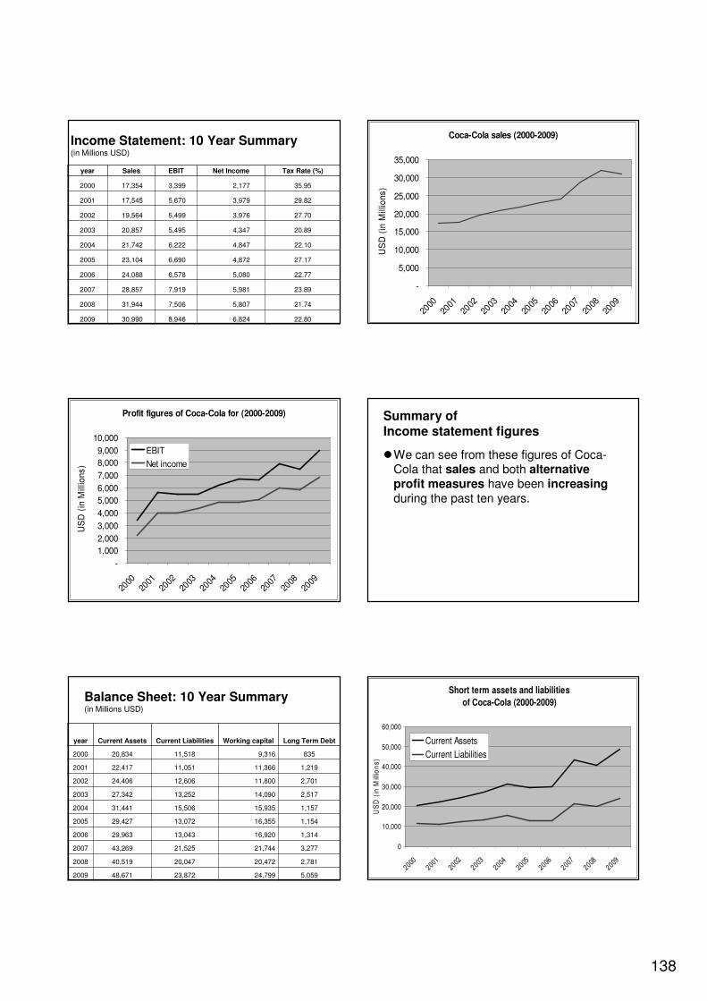
138
Income Statement: 10 Year Summary(in Millions USD)
22.806,824 8,946 30,990 2009
21.745,807 7,506 31,944 2008
23.895,981 7,919 28,857 2007
22.775,080 6,578 24,088 2006
27.174,872 6,690 23,104 2005
22.104,847 6,222 21,742 2004
20.894,347 5,495 20,857 2003
27.703,976 5,499 19,564 2002
29.823,979 5,670 17,545 2001
35.952,177 3,399 17,354 2000
Tax Rate (%)Net IncomeEBITSalesyear
Coca-Cola sales (2000-2009)
-
5,000
10,000
15,000
20,000
25,000
30,000
35,000
2000
2001
2002
2003
2004
2005
2006
2007
2008
2009
US
D (
in M
illio
ns
)
Profit figures of Coca-Cola for (2000-2009)
-
1,000
2,000
3,000
4,000
5,000
6,000
7,000
8,000
9,000
10,000
2000
2001
2002
2003
2004
2005
2006
2007
2008
2009
US
D (
in M
illio
ns
)
EBIT
Net income
Summary of Income statement figures
�We can see from these figures of Coca-Cola that sales and both alternative profit measures have been increasingduring the past ten years.
Balance Sheet: 10 Year Summary(in Millions USD)
5,05924,79923,87248,6712009
2,78120,47220,04740,5192008
3,27721,74421,52543,2692007
1,31416,92013,04329,9632006
1,15416,35513,07229,4272005
1,15715,93515,50631,4412004
2,51714,09013,25227,3422003
2,70111,80012,60624,4062002
1,21911,36611,05122,4172001
8359,31611,51820,8342000
Long Term DebtWorking capitalCurrent LiabilitiesCurrent Assetsyear
Short term assets and liabilities
of Coca-Cola (2000-2009)
0
10,000
20,000
30,000
40,000
50,000
60,000
20002001
2002
20032004
20052006
20072008
2009
US
D (
in M
illio
ns
)
Current Assets
Current Liabilities
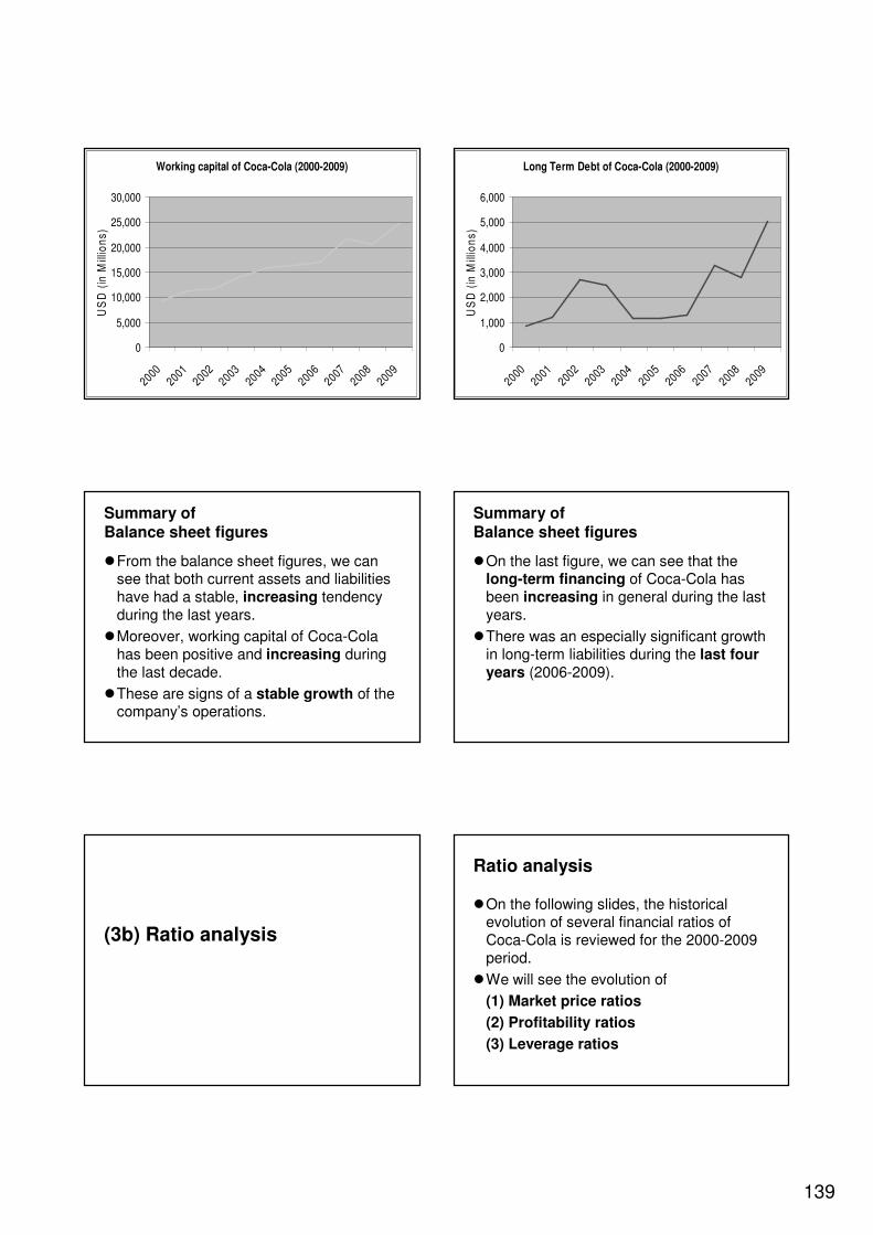
139
Working capital of Coca-Cola (2000-2009)
0
5,000
10,000
15,000
20,000
25,000
30,000
20002001
20022003
2004
2005
2006
20072008
2009
US
D (
in M
illio
ns
)
Long Term Debt of Coca-Cola (2000-2009)
0
1,000
2,000
3,000
4,000
5,000
6,000
20002001
2002
2003
20042005
2006
2007
20082009
US
D (
in M
illio
ns
)
Summary of Balance sheet figures
�From the balance sheet figures, we can see that both current assets and liabilities have had a stable, increasing tendency during the last years.
�Moreover, working capital of Coca-Cola has been positive and increasing during the last decade.
�These are signs of a stable growth of the company’s operations.
Summary of Balance sheet figures
�On the last figure, we can see that the long-term financing of Coca-Cola has been increasing in general during the last years.
�There was an especially significant growth in long-term liabilities during the last four years (2006-2009).
(3b) Ratio analysis
Ratio analysis
�On the following slides, the historical evolution of several financial ratios of Coca-Cola is reviewed for the 2000-2009 period.
�We will see the evolution of
(1) Market price ratios
(2) Profitability ratios
(3) Leverage ratios

140
(1) Market price ratios
5.294.2816.72009
5.113.3121.62008
6.544.96212007
6.614.7120.32006
5.844.18212005
6.34.6523.32004
8.795.99252003
9.185.5631.12002
10.316.6830.42001
16.258.7632000
Price/BookPrice/SalesAverage P/Eyear
Average P/E ratio of Coca-Cola (2000-2009)
0
10
20
30
40
50
60
70
2000
20012002
2003
2004
2005200
620
072008
2009
Market price ratios of Coca-Cola (2000-2009)
0
2
4
6
8
10
12
14
16
18
2000
2001
2002
2003
2004
2005
2006
2007
2008
2009
Price/Sales
Price/Book
Summary of Market price ratios
�We can see that the P/E, P/Sales and P/Book value ratios of Coca-Cola have been decreasing during 2000-2009.
� Interpretation: Most analysts believe that low P/E stocks are more attractive than high P/E stocks because they allow the investor to pay less USD of current earnings.
�The same positive conclusion can obtained looking at the P/Sales and P/Book value ratios.
(2) Profitability ratios
2.930.2914.0027.502009
2.490.2314.3028.402008
2.570.2713.8027.502007
2.160.2717.0030.002006
2.040.2916.6029.802005
2.000.2915.4030.402004
1.770.2615.9030.902003
1.600.2816.3033.702002
1.600.3217.7035.002001
0.880.2010.4023.402000
EPSROSROAROEyear
Profitability ratios of Coca-Cola (2000-2009)
0
5
10
15
20
25
30
35
40
20002001
20022003
20042005
20062007
20082009
%
Return on Equity
Return on Assets

141
Coca-Cola return on sales (ROS) ratio
-
0.05
0.10
0.15
0.20
0.25
0.30
0.35
2000
2001
2002
2003
2004
2005
2006
2007
2008
2009
%
Coca-Cola earnings per share (EPS) ratio (2000-2009)
0.00
0.50
1.00
1.50
2.00
2.50
3.00
3.50
2000
2001
2002
2003
2004
2005
2006
2007
2008
2009
US
D
Summary of profitability ratios
�We can see that ROE and ROA have been decreasing and ROS has been relatively stable during 2000-2009.
� In the same time, EPS has been increasing significantly.
�The last point seems to be contradictory but remember the way ROE and EPS are computed:
ROE = Net income / Equity
EPS = Net income / # common shares
Summary of profitability ratios
�Previously, we saw that Coca-Cola net income increased very significantly from 2,177 Millions USD to 6,824 Millions USD.
�The evolution of ROE can be explained by the fact that the denominator of ROE (i.e., equity) was increasing faster than Net income.
�The significant evolution of EPS is also motivated by the fact that the denominator of EPS (i.e., number of common shares outstanding) was significantly decreasing.
Summary of profitability ratios
�The decreasing tendency of number of common shares can be explained by the fact that Coca-Cola repurchased own shares on the market during the last years.
�These shares are represented in the Equity section of Balance with negative values on the following account:
�Treasury stock – Common (Millions USD):
(25,398)(24,213)(23,375)(22,118)(19,644)
31/12/200931/12/200831/12/200731/12/200631/12/2005
Summary of profitability ratios
�This own share repurchase resulted in a concentration of common sharesamong outstanding shareholders.
� It increased the net income per shares outstanding (i.e., EPS increased).
�Another consequence of repurchasing own shares has been the increasing book value per common share presented on the next figure:
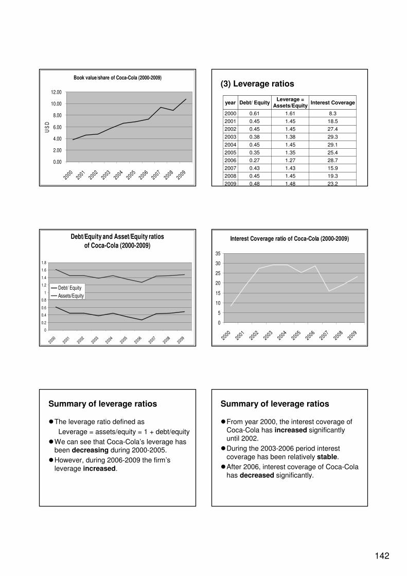
142
Book value/share of Coca-Cola (2000-2009)
0.00
2.00
4.00
6.00
8.00
10.00
12.00
20002001
20022003
20042005
20062007
20082009
US
D
(3) Leverage ratios
23.21.480.482009
19.31.450.452008
15.91.430.432007
28.71.270.272006
25.41.350.352005
29.11.450.452004
29.31.380.382003
27.41.450.452002
18.51.450.452001
8.31.610.612000
Interest CoverageLeverage =
Assets/EquityDebt/ Equityyear
Debt/Equity and Asset/Equity ratios
of Coca-Cola (2000-2009)
0
0.2
0.4
0.6
0.8
1
1.2
1.4
1.6
1.8
20002001
20022003
20042005
20062007
20082009
Debt/ Equity
Assets/Equity
Interest Coverage ratio of Coca-Cola (2000-2009)
0
5
10
15
20
25
30
35
2000
2001
2002
20032004
20052006
20072008
2009
Summary of leverage ratios
�The leverage ratio defined as
Leverage = assets/equity = 1 + debt/equity
�We can see that Coca-Cola’s leverage has been decreasing during 2000-2005.
�However, during 2006-2009 the firm’s leverage increased.
Summary of leverage ratios
�From year 2000, the interest coverage of Coca-Cola has increased significantly until 2002.
�During the 2003-2006 period interest coverage has been relatively stable.
�After 2006, interest coverage of Coca-Cola has decreased significantly.

143
(4) Comparison with other firms
Comparison of financial ratios
�On the following slides, we compare several ratios of Coca-Cola to the
(1) Industry average and
(2) S&P500 firms’ average.
�This way we can compare various aspects of Coca-Cola financial performance to that of its competitors and other firms in the U.S. economy represented by the S&P500 index.
Comparison of financial ratios
�We review several ratios in the following structure:
(1) Growth rates of some accounts of the Income statement
(2) Profitability ratios
(3) Profit margins
(4) Market price ratios
(5) Leverage and liquidity ratios
(6) Efficiency ratios
Comparison of financial ratios
� In the following tables, we can observe several ratios for each group.
�Note: When the exact time of the ratio is not specified clearly then it will mean the last year (2009) figures.
Growth rates (Income statement)
4.978.9310.4Dividends (5-Year Annual Avg.)
8.248.997.08Net Income (5-Year Annual Avg.)
7.758.847.35Sales (5-Year Annual Avg.)
14.318.517.5Net Income
10.765.4Sales
S&P 500IndustryCompanyGrowth Rates %
Profitability ratios
10.317.823ROIC (5-Year Average)
7.612.315.7ROA (5-Year Average)
16.222.529.8ROE (5-Year Average)
9.418.522.4ROIC
6.912.715.5ROA
20.738.830.2ROE
S&P 500IndustryCompanyInvestment Returns %
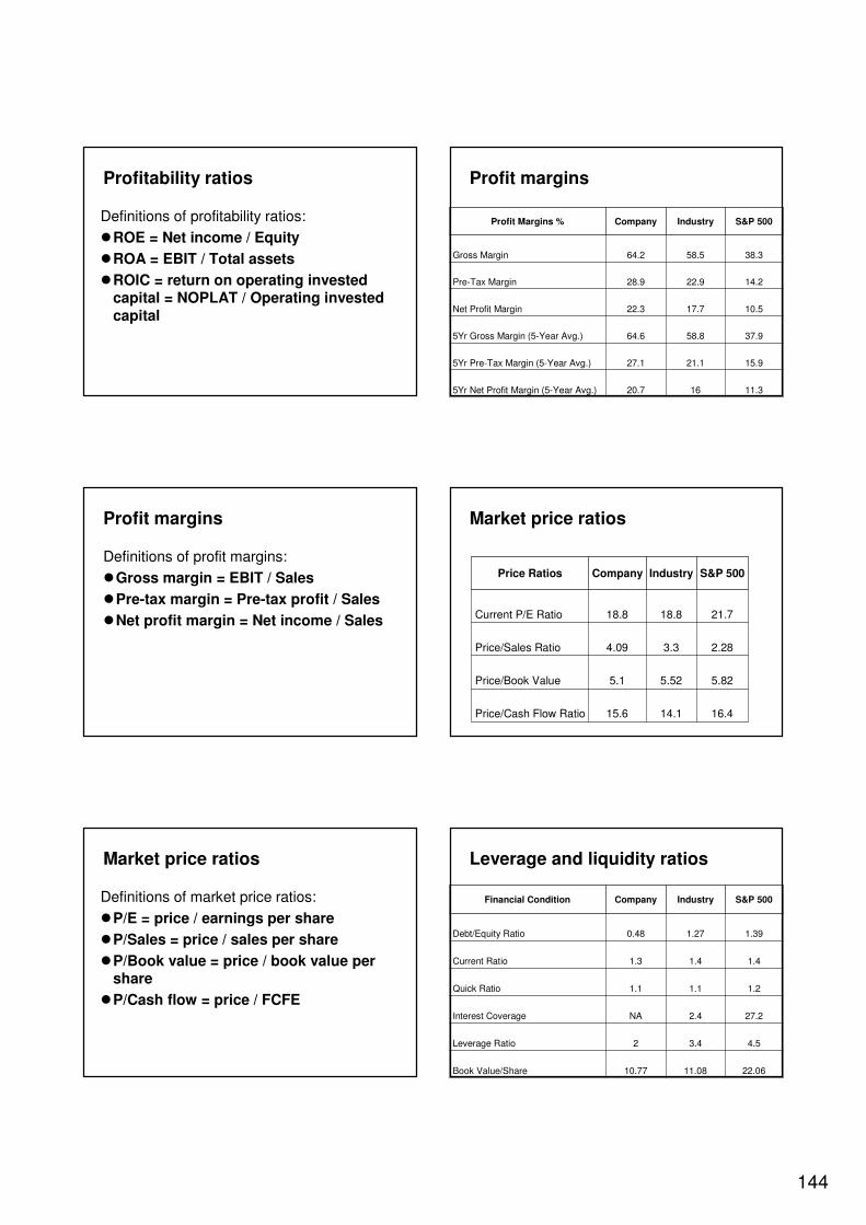
144
Profitability ratios
Definitions of profitability ratios:
�ROE = Net income / Equity
�ROA = EBIT / Total assets
�ROIC = return on operating invested capital = NOPLAT / Operating invested capital
Profit margins
11.31620.75Yr Net Profit Margin (5-Year Avg.)
15.921.127.15Yr Pre-Tax Margin (5-Year Avg.)
37.958.864.65Yr Gross Margin (5-Year Avg.)
10.517.722.3Net Profit Margin
14.222.928.9Pre-Tax Margin
38.358.564.2Gross Margin
S&P 500IndustryCompanyProfit Margins %
Profit margins
Definitions of profit margins:
�Gross margin = EBIT / Sales
�Pre-tax margin = Pre-tax profit / Sales
�Net profit margin = Net income / Sales
Market price ratios
16.414.115.6Price/Cash Flow Ratio
5.825.525.1Price/Book Value
2.283.34.09Price/Sales Ratio
21.718.818.8Current P/E Ratio
S&P 500IndustryCompanyPrice Ratios
Market price ratios
Definitions of market price ratios:
�P/E = price / earnings per share
�P/Sales = price / sales per share
�P/Book value = price / book value per share
�P/Cash flow = price / FCFE
Leverage and liquidity ratios
22.0611.0810.77Book Value/Share
4.53.42Leverage Ratio
27.22.4NAInterest Coverage
1.21.11.1Quick Ratio
1.41.41.3Current Ratio
1.391.270.48Debt/Equity Ratio
S&P 500IndustryCompanyFinancial Condition

145
Leverage and liquidity ratios
Definitions of leverage and liquidity ratios:
�Current ratio = current assets / current liabilities
�Quick ratio = (cash + marketable securities + receivables) / current liabilities
� Interest coverage = EBIT / interest expense
�Leverage = assets / equity
Efficiency ratios
0.80.80.7Asset Turnover
9.26.74.9Inventory Turnover
14.410.29.1Receivable Turnover
814,514334,062333,944Sales/Employee
75,39762,52174,418Net income/Employee
S&P 500IndustryCompanyManagement Efficiency
Efficiency ratios
Definitions of efficiency ratios:
�Receivable turnover = Cost of goods sold / receivables
� Inventory turnover = Cost of goods sold / inventories
�Asset turnover = Sales / total assets
(5) Forecasting FCF
Forecasting FCF
�Using accounting information downloaded from www.msn.com, the Balance sheets and Income statements were constructed for the last five years: 2005-2009.
Forecasting FCF
�The following three slides show the structure of the:
(1) Balance sheet: Assets
(2) Balance sheet: Liabilities and equity
(3) Income statement

146
Other Assets, Total
Other Long Term Assets, Total
Note Receivable - Long Term
Long Term Investments
Intangibles, Net
Goodwill, Net
Property/Plant/Equipment, Total - Net
Total fixed assets
Other Current Assets, Total
Prepaid Expenses
Total Inventory
Total Receivables, Net
Cash and Short Term Investments
Total Current Assets
Assets
Other Equity, Total
Treasury Stock - Common
Retained Earnings (Accumulated Deficit)
Additional Paid-In Capital
Common Stock
Preferred Stock - Non Redeemable, Net
Redeemable Preferred Stock
Total Equity
Other Liabilities, Total
Minority Interest
Deferred Income Tax
Total Long Term Debt
Total long-term liabilities
Other Current Liabilities, Total
Current Port. of LT Debt/Capital Leases
Notes Payable/Short Term Debt
Accrued Expenses
Payable/Accrued
Accounts Payable
Total Current Liabilities
Total liabilities
Liabilities and Shareholders' Equity
Net Income
U.S. GAAP Adjustment
Equity In Affiliates
Minority Interest
Income Tax - Total
Income Before Tax
Extraordinary result
Other, Net
Gain (Loss) on Sale of Assets
Unusual Expense (Income)
Financial result
Interest Income (Expense), Net Non-Operating
EBIT
Depreciation/Amortization
EBITDA
Other Operating Expenses, Total
Interest Expense (Income), Net Operating
Research & Development
Selling/General/Administrative Expenses, Total
Gross Profit
Cost of Revenue, Total
Total Revenue
Forecasting FCF
�We shall forecast the cash flow statement as follows:
�First, we forecast the Balance sheet and the Income statement for six years.
�The first five years define the explicit forecast period.
�The sixth year is the starting year of the continuing value period.
Forecasting Balance sheet
�To forecast the Balance sheet, we simply computed the percentage of each account to total assets during the past 5 years.
�Then, we identified the relatively stable percentages and computed the average percentage of the account over the stable period.
Forecasting Balance sheet
�Then, we assumed that the value of total assets will grow according to the GDP growth rate of the U.S.
�We assumed 3 percent for the U.S. growth rate and forecasted total assets for the next six years.
�Finally, we used the percentage averages of single accounts to compute the forecasted value of each account in the Balance sheet.
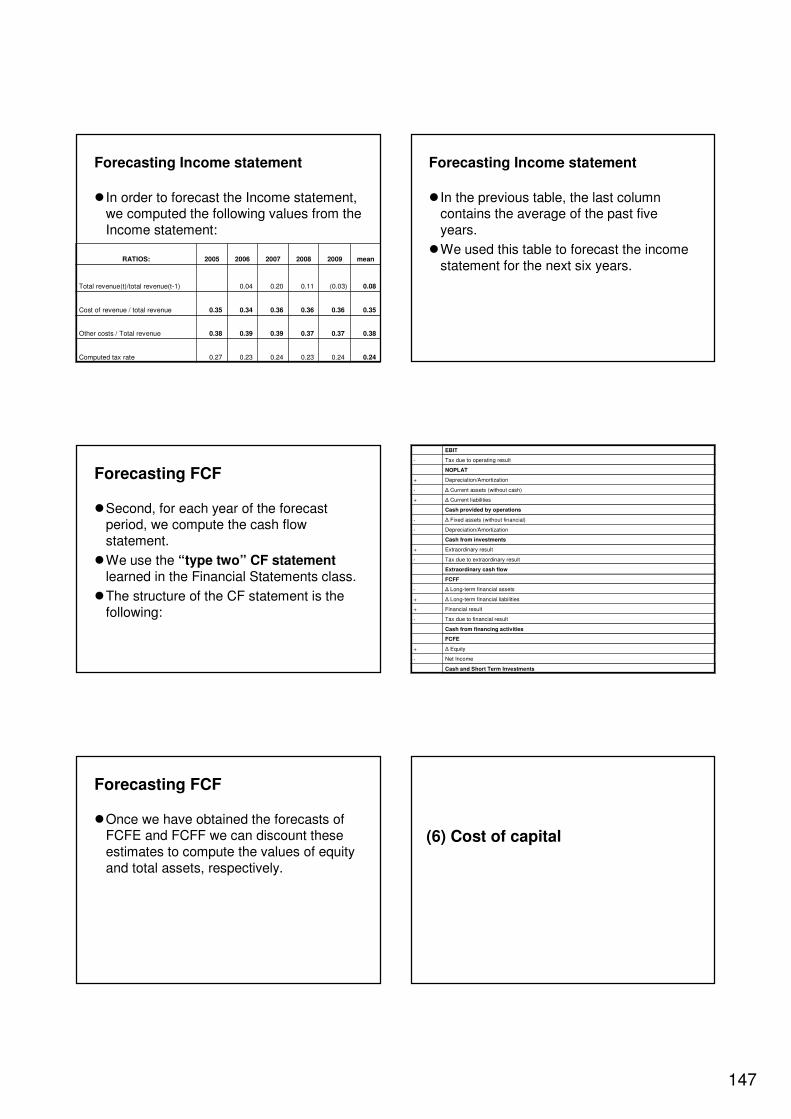
147
Forecasting Income statement
� In order to forecast the Income statement, we computed the following values from the Income statement:
0.24 0.24 0.23 0.24 0.23 0.27 Computed tax rate
0.38 0.37 0.37 0.39 0.39 0.38 Other costs / Total revenue
0.35 0.36 0.36 0.36 0.34 0.35 Cost of revenue / total revenue
0.08 (0.03)0.11 0.20 0.04 Total revenue(t)/total revenue(t-1)
mean20092008200720062005RATIOS:
Forecasting Income statement
� In the previous table, the last column contains the average of the past five years.
�We used this table to forecast the income statement for the next six years.
Forecasting FCF
�Second, for each year of the forecast period, we compute the cash flow statement.
�We use the “type two” CF statementlearned in the Financial Statements class.
�The structure of the CF statement is the following:
Cash and Short Term Investments
Net Income-
∆ Equity+
FCFE
Cash from financing activities
Tax due to financial result-
Financial result+
∆ Long-term financial liabilities+
∆ Long-term financial assets-
FCFF
Extraordinary cash flow
Tax due to extraordinary result-
Extraordinary result+
Cash from investments
Depreciation/Amortization-
∆ Fixed assets (without financial)-
Cash provided by operations
∆ Current liabilities+
∆ Current assets (without cash)-
Depreciation/Amortization+
NOPLAT
Tax due to operating result-
EBIT
Forecasting FCF
�Once we have obtained the forecasts of FCFE and FCFF we can discount these estimates to compute the values of equity and total assets, respectively.
(6) Cost of capital
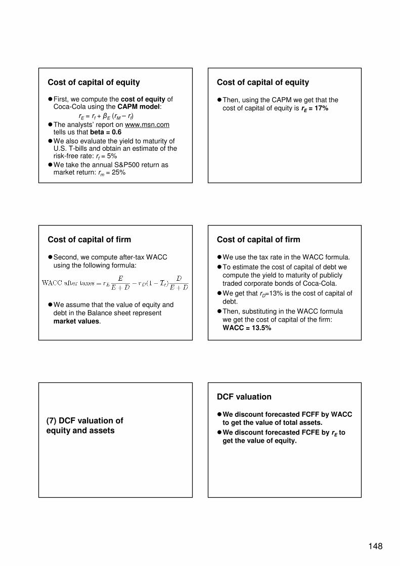
148
Cost of capital of equity
�First, we compute the cost of equity of Coca-Cola using the CAPM model:
rE = rf + βE (rM – rf)
�The analysts’ report on www.msn.comtells us that beta = 0.6
�We also evaluate the yield to maturity of U.S. T-bills and obtain an estimate of the risk-free rate: rf = 5%
�We take the annual S&P500 return as market return: rm = 25%
Cost of capital of equity
�Then, using the CAPM we get that the cost of capital of equity is rE = 17%
Cost of capital of firm
�Second, we compute after-tax WACC using the following formula:
�We assume that the value of equity and debt in the Balance sheet represent market values.
Cost of capital of firm
�We use the tax rate in the WACC formula.
�To estimate the cost of capital of debt we compute the yield to maturity of publicly traded corporate bonds of Coca-Cola.
�We get that rD=13% is the cost of capital of debt.
�Then, substituting in the WACC formula we get the cost of capital of the firm: WACC = 13.5%
(7) DCF valuation of equity and assets
DCF valuation
�We discount forecasted FCFF by WACC to get the value of total assets.
�We discount forecasted FCFE by rE to get the value of equity.

149
DCF valuation
�For the explicit forecast period the next present value formulas are used:
PV(FCFEt) = FCFEt / (1+rE)t
PV(FCFFt) = FCFFt / (1+WACC)t
DCF valuation
�For the continuing value forecast periodwe assume that CF forms a growing perpetuity.
�The growth rate, g is assumed to be 1.5%
�We use the following formula to compute the present value of the growing perpetuities:
PV(continuing value) = CF6/[(r-g)(1+r)5]
DCF valuation
�As a summary, we present the present value formulas for the FCFE and FCFF cash flows:
DCF valuation: Summary
� We can compare to DCF valuation result with the balance sheet items in the following table:
23,872 16,302 Value of debt
48,671 65,166 Value of assets
24,799 48,865 Value of equity
BALANCEDCFSUMMARY:


![István Elek - {Iconip} - [2012]](https://static.fdocuments.in/doc/165x107/577ce4c71a28abf1038f244f/istvan-elek-iconip-2012.jpg)