SyteLine Forecasting System Implementation Guide V8 · Page 1 SyteLine Forecasting System...

SyteLine

Forecasting System

Implementation

Guide

V8

Business Technology Associates

5910 Courtyard Drive, Suite 200 Austin, TX 78731

Phone: (512) 343-9600

Web: www.btasystems.com Email: [email protected]

http://www.btasystems.com/

mailto:[email protected]

Table of Contents

Section 1 – Quick Start Guide Page 3

Section 2- Forecasting Overview Page 7

Section 3 – System Set-Up Page 9

Forecast Parameters

Planning Parameters

Accounting Periods

Forecast History

Section 4 – Creating and Working with Forecasts Page 16

Details of Forecast Form

Header

History Tab

Calculation Tab

Adding New Items

Manipulating Individual Items

Manipulating Groups of Items

Pushing the Forecast to the Planning Engine

Section 5– Activities Page 26

Safety Stock Maintenance

Forecast As

Forecast Extended History

Forecast Parameter Maintenance

Section 6 – Utilities Page 30

Auto Calculate Forecast for All Items

Forecast Create Initial Forecast

Forecast Monthly Utility

Update MRP for All Items

Update Review Date for All Items

Section 7 – Enhanced Functions Page 34

Planning BoM

Useage Base Consumption

Forecasting in Fiscal Periods

Section 8 – System Update Page 37

Daily/Weekly/Monthly Activities

Exception Messaging

Section 9 – Frequently Used Reports Page 39

Appendix A- Forecasting Models Page 40

Appendix B- Forecasting FAQ’s Page 43

Appendix C – Demand Filter and Track Limit Page 45

Appendix D – Order Minimum and Safety Stock Calculations Page 47

SECTION 1 – Quick Start Guide Overview:

1. Develop Forecast Parameters

a. FIELD DESCRIPTIONS

i. MRP Interface: Choose Yes to allow Forecasts to move to the Planning Engine ii. Load MRP Freq: Load MRP Frequency can be Monthly,or Weekly. The Forecast

will be loaded into MRP based on this frequency. iii. Load MRP Timing: If your MRP Frequency is Monthly, then enter the day of

the month (06) and if your MRP Frequency is Weekly enter the week day (MON). It determines when the Forecast will be due.

iv. Date to Use for History – When the monthly utility gathers data, Which date should it use for the BOOKING date – the Customer Order Line Due Date or the Customer Order Date . Select “Order Date” or “Due Date”

v. Calendar Type – select Fiscal or Calendar. Selecting Fiscal allows processing forecast in periods tied to the Accounting Periods

vi. Fiscal Period – if “Fiscal” is slected in Calendar type – enter the number of periods in the Accounting Periods form.

vii. Testing Run Date – make sure this is blank

Develop Forecast

Parameters

Add Forecast

Items

Create Forecast Push Forecast to

Planning Engine

SECTION 1 – Quick Start Guide (Con’t)

2. Enter Forecast Items to Forecast Main Form a. New Record - Enter Item in Forecast Main and Save

i. System gathers and displays history.

3. The History displays in the history chart. This information is displayed in the default of units booked by date.

4. The history is collected based on the settings in the Forecast Parameters form.


6. Create Initial Forecast Values

a. Select the Calculations Tab b. In the Model field, select “Automatic Selection” or pick a model

i. Automatic Selection will create a recommendation for a Model based on fit criteria

c. Push “Auto Calc Fcst” d. The calculated values are represented in the blue “Forecast” column in the lower right

hand corner. e. The numbers that will flow to the planning Engine are represented in the Green “Net

Forcast” column in the lower right hand corner.


f. Push “Graph” button for “Forecast Graph”

g. If this appears to be an acceptable forecast, save the record. If not acceptable, repeat steps 5b-5e

7. Push the Forecast to the Planning Engine. a. Select the “Update MRP“ button to Populate the Forecast Form in SyteLine with the

calculated Forecast.

8. Repeat Steps 2 – 4 until each item you choose to forecast is a member of the Forecast table. Please note: There are several methods to load large datasets – please see “Section 3 – Setup” for details on load instructions.

SECTION 2 – Forecasting Overview

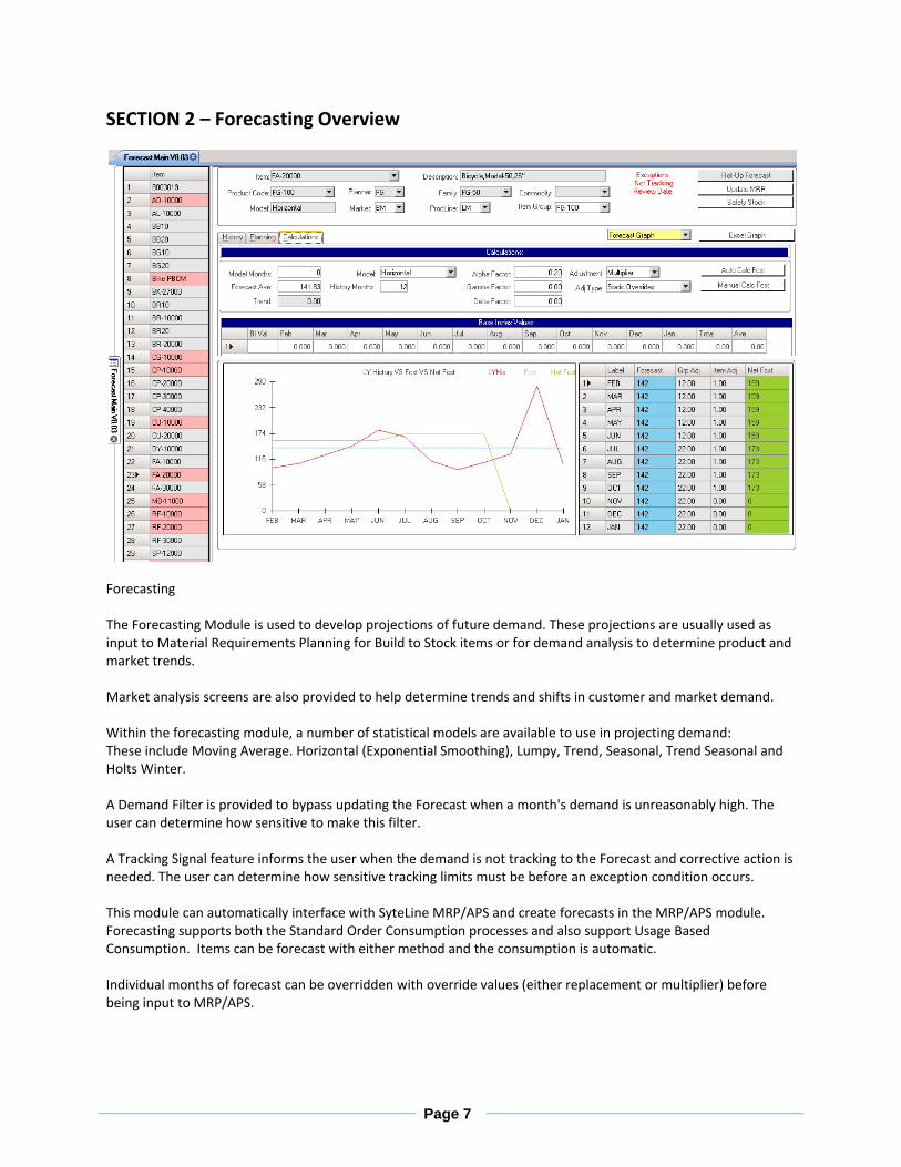
Forecasting The Forecasting Module is used to develop projections of future demand. These projections are usually used as input to Material Requirements Planning for Build to Stock items or for demand analysis to determine product and market trends. Market analysis screens are also provided to help determine trends and shifts in customer and market demand. Within the forecasting module, a number of statistical models are available to use in projecting demand: These include Moving Average. Horizontal (Exponential Smoothing), Lumpy, Trend, Seasonal, Trend Seasonal and Holts Winter. A Demand Filter is provided to bypass updating the Forecast when a month's demand is unreasonably high. The user can determine how sensitive to make this filter. A Tracking Signal feature informs the user when the demand is not tracking to the Forecast and corrective action is needed. The user can determine how sensitive tracking limits must be before an exception condition occurs. This module can automatically interface with SyteLine MRP/APS and create forecasts in the MRP/APS module. Forecasting supports both the Standard Order Consumption processes and also support Usage Based Consumption. Items can be forecast with either method and the consumption is automatic. Individual months of forecast can be overridden with override values (either replacement or multiplier) before being input to MRP/APS.

SECTION 2 – Forecasting Overview - Con’t SyteLine Forecasting Automatically calculates new forecasts and exception conditions.

SyteLine Forecasting Automatically updates MRP/APS with the new forecasts (including any overrides

you may have chosen to use)

SyteLine Forecasting supports both Fiscal and Calendar Forecasting and Reporting.

The Forecasting module supports the use of planning bills of material including consumption algorithms

to eliminate the manual process of adjusting your planning BoM forecast for actual sales.

Forecasting is a comhrensive demand management tool. It can be used to automatically select the best

statistical model at the item level or it can be used to store your user input forecasts for automatic

update of MRP/APS.

SECTION 3 – System Set-Up

Forecasting Parameters

The forecasting parameters screen contains basic settings which will govern how the forecasting

application functions at your company.

The form has three tabs.

General – overall functions of the program

Transaction Types – details the type of data to gather during History Data collection

Collaborative – reserved for future use

1. General TabField Descriptions are as follows:

a. MRP Interface: This logical field gives the user the choice to enable (Choose Yes to enable) an on-

line transfer of forecasts from the forecasting application to the SyteLine Forecast Form.

b. Load MRP Freq: Load MRP Frequency can be Monthly or Weekly. The Forecast will be loaded into MRP/APS based on this frequency.

c. Load MRP Timing: Equal to the day of the month (06) for Monthly and to the week day (Monday) for Weekly. It determines when the Forecast will be due.

d. Usage Forecast Look Ahead: Enter the number of days to look forward for consumption of Forecast – used for Usage Type data.

e. Usage Forecast Look Behind: Enter the number of days to look behind for consumption of Forecast – used for Usage Type data

SECTION 3 – System Set-Up – Con’t

f. Forecast Output Periods – reserved for future use g. Date to Use for History – Used when importing data into the system. Choose Order Date or Due

Date to determine if you want history to be based on the date the order was taken, or when the order was due.

h. Use Ext History for Create Init Fcst: Selecting Yes indicates that you want the system to gather data from the Extended History tables when creating an initial forecast. See “Section 6 – Create Initial Forecast” for more information.

a. Calendar Type – select Fiscal or Calendar. Selecting Fiscal allows processing forecast in periods tied to the Accounting Periods

i. Fiscal Period – if “Fiscal” is slected in Calendar type – enter the number of periods in the Accounting Periods form

j. Testing Run Date: Used to override the current system date. Use caution when updating this field. It can be used to recalculate forecasts when one or more months were skipped.

k. Job Setup Cost Addl: The dollar amount entered in this field is used by the system as an input to the order minimum calculations. This cost is in addition to any setup charges that are defined in the item’s current routing.

l. Purch Order Setup Addl: The dollar amount entered in this field is used by the system as an input to the order minimum calculations.

m. Inventory Carrying Rate: This percentage is the Annual estimated cost of carrying inventory. Example: If your company uses 20% as the estimated cost of carrying inventory enter .2 in this field. Again, this percentage is used by the system as an input to the order minimum calculations.

n. Default Service Level. A desired measure (expressed as a percentage) of satisfying demand through inventory or by the current production schedule in time to satisfy the customer’s requested delivery date and quantities. In a make to stock environment, service level is sometimes calculated as the percentage of orders picked complete from stock upon receipt of the customer order, the percentage of line items picked complete, or the percentage of total dollar demand picked complete. In make to order and design-to-order environments, service level is the percentage of time that the customer requested or acknowledged date was met by shipping complete product quantities.

o. Item Group: Can be Product Code, Family Code or Neither. Logical field used to determine which code is to be used for the Item Group.

p. User Label 1: Used to determine what label to apply to label 1 when used with Group Memberships

q. User Label 2: Used to determine what label to apply to label 2. r. Top Customer Reports Dollar Limit: Enter the dollar value to determine the extraction of

records for the Top Customers Reports s. Display Notes Automatically – notes can be made to show when you select an item from the

Forecast Main form – to show automatically, select the box t. Level Load – use of this functionality will take the forecast calculated in a period of time and

“level” the forecast across the periods.


2. Transaction Types – a forecasted item can use two types of data for History. We may want to use

different types of history as the basis for creating a statistical forecast. You must select “Usage” for items that will utilize “Usage Base Consumption” functionality

a. Orders – this is historical data associated with the Sales History of items b. Usage – this is historical data associated with the Use of an item (including Sales Orders)

c. Select ing a Transaction Type at an item level will then default to this parameter form when identifying which tables will be selected when the history collection process takes place.


SyteLine Planning Parameters

1. Use CO or Forecast - Determines whether to use Customer Orders, Forecasts or both as drivers of demand.

2. Forecast Look Ahead/Behind - This parameter lets you set the number of days into the past/ future to look for forecasts to be consumed by customer orders during MRP or APS regeneration.

When a customer order is entered in Order Entry, the system begins at the customer order item due date and looks this number of manufacturing days into the future/or the past for forecast orders to be consumed by the customer order. The system always looks back first, then forward. The Look Behind number also determines how long a forecast will be valid. The numbers are in Manufacturing days. These values can also be set and maintained at the Product Code Level


Accounting Periods

a. If you are going to use Fiscal Periods to forecast (use your Fiscal Periods versus 12 Calendar

months) then you must set up at least 5 Fiscal Years in the past.

Importing History Data

1. Calculations of a Regression Model forecast are dependent on historical information of sales available

prior to the calculation. It is recommended that a minimum of 3 years worth of history be available

to create the forecast.

2. Existing Users with less than 3 years of data and new customer can import history from an external

source utilizing the Extended History form.

3. For Data Sets less than 20,000 records use the Extended History Format

4. For Data Sets greater than 20,000 records consider consolidating the data into monthly buckets for

the import.


Extended History

1. FIELD DESCRIPTIONS

a. Transaction Date: Enter the Dates with which you want the information to post into Forecast History

b. Post To History – Used to begin the posting transaction c. Filename – the location of the history data d. Import Button -To import data into this form from a .CSV file (Vault) Delete All Records First –

check this box to delete all data in the table prior to importing new records. e. Item – Any item number can be stored in the Extended History table, including items not found

in the SyteLine Items Form. If the Item does not exist in the Forecast Main form, then the Item’s history will not load when the post button is selected.

f. Type - Enter the Type of record you are importing. B = Booking Quantity, C=Booking $ Value, S=Shipment Qty, T= Shipment $ Value

g. Date - Date in which the qty and extended price will be posted to on the History Form. h. Qty - Qty to update the history with i. Ext Price - price for History types that use Price instead of qty j. Cust Num - Special Format Customer Num for sorting and storing data. k. CO Num - Special Format Customer Order Num for sorting and storing data. l. CO Line - Special Format Customer Order Line for sorting and storing data.


2. FORM FUNCTIONALITY

a. You need not have all the information in the fields, but you have to have the headers on the

spreadsheet. Clean the data before it goes into the file. Data that you must have:

i. Item – Does not have to be a SyteLine item. ii. Type

iii. Date iv. Qty

NOTE: The import assumes one header row, so anything on the first line of the spreadsheet will

be skipped.

b. Save the file as .csv. c. Make sure that you keep a copy of the file to have a history of what was imported.

d. Import. e. Post To History Button

i. Note – “Delete All Records First” will delete all history in the vault.

ii. Note – the “Item” needs to be resident in Forecast Main. To do this:

1. Add one item at a time and save – see Quick Start Section of the manual.

2. Run the “Create Initial Forecast” utility – see Utilities Section of the manual.

SECTION 4 – CREATING AND WORKING WITH FORECASTS

DETAILS OF THE FORECAST MAIN FORM

1. Header Information

i. Item - Item Number – Must be a SyteLine Item number. ii. Description - Item's Description

iii. Product Code - Item's Product Code iv. Family Code – Family Code from Items form v. Planner - Planner Code from Items form

vi. Commodity - Commodity Code from Items form vii. Model – Current selected Forecast Model

viii. User Defined Field 1 – shown as Market ix. User Defined Field 2 – shown as ProdLine

x. Item Group SECTION 4 – CREATING AND WORKING WITH FORECASTS – Con’t 2. History Tab

i. History Identification Bar - Displays the current history units and level.

ii. Demand History - Last 4 years and current year of demand history by month with year totals

and year average. This information is kept in four formats:

a. Booked Quantities b. Booked Net Sales Dollars c. Shipped Quantities d. Shipped Net Sales Dollars

iii. Excel Graph – Used for Graphing History and Forecast information

SECTION 4 – CREATING AND WORKING WITH FORECASTS – Con’t

iv. Quick History Gaph – shows Last Years Consumption (LYHis), Current Calculated Forecast (Fcst), and Net Forecast (Net Fcst)

v. The Forecast Data box shows 1. Period of Forecast 2. Calculated/Derived Forecast 3. The Group Adj represents any Group Adjustments to the item 4. The Item Adj represents any Item Adjustments to the item 5. The Green Line column represents the adjusted forecast that will be applied to

MRP/APS.


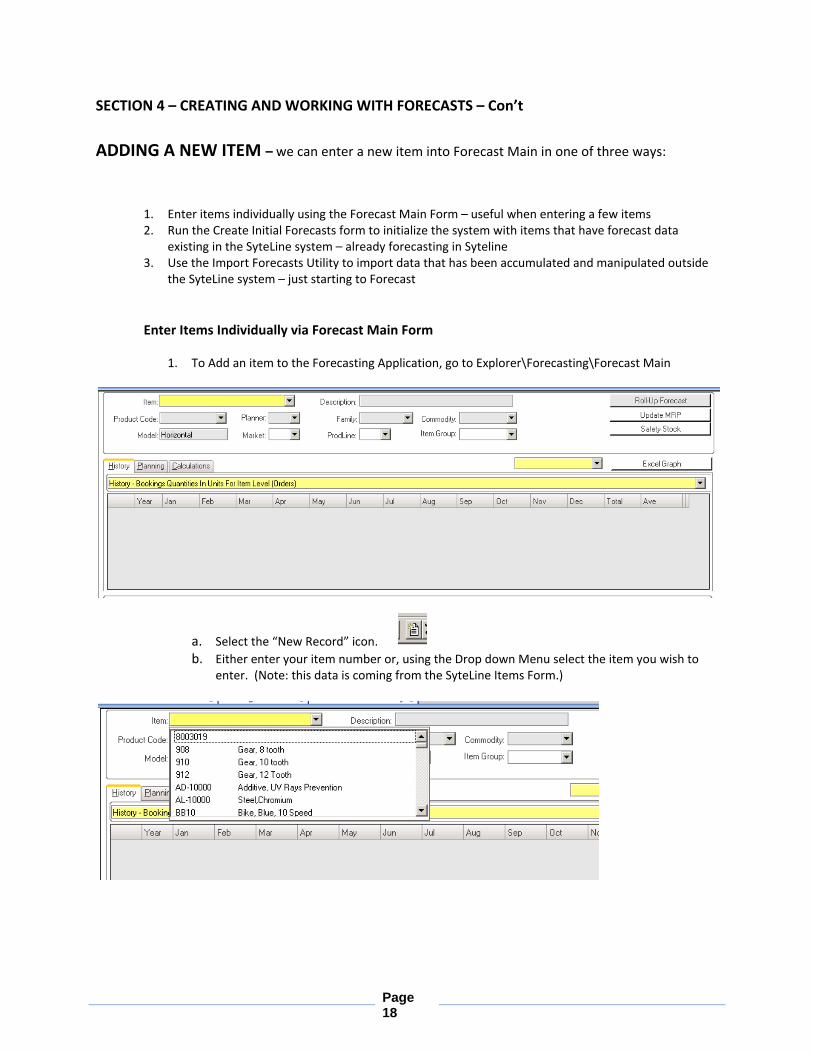
ADDING A NEW ITEM – we can enter a new item into Forecast Main in one of three ways:

1. Enter items individually using the Forecast Main Form – useful when entering a few items 2. Run the Create Initial Forecasts form to initialize the system with items that have forecast data

existing in the SyteLine system – already forecasting in Syteline 3. Use the Import Forecasts Utility to import data that has been accumulated and manipulated outside

the SyteLine system – just starting to Forecast

Enter Items Individually via Forecast Main Form

1. To Add an item to the Forecasting Application, go to Explorer\Forecasting\Forecast Main

a. Select the “New Record” icon. b. Either enter your item number or, using the Drop down Menu select the item you wish to

enter. (Note: this data is coming from the SyteLine Items Form.)


c. Go to the Planning Tab enter whether you want the forecast generation to be based on Customer Orders or based on Usage data. For example, a service item might be forecast based on customer orders. In this way we forecast the demand directly from sales along with any dependent demand coming from production forecasts.

d. Save the Record e. The system will populate the history tables with data (bookings and shipments, dollars and

units) f. This item is now a member of the forecast items family but does not have a forecast.

g. Optionally consider whether this item will be “Planned” (passed to the Forecast form) as weekly or monthly quantities. Directly beneath the Data Type field are the Freq and Timing Fields. These values default from Forecasting Parameters if you leave the fields blank here.. If you wish to override these defaults at the item level you would do so here.


Create Initial Forecasts Utility

1. Open form: Forecast Create Initial Forecasts 2. This form has two different forecast import utilities. One imports items based on the fact that you

are selling them and the other performs and import based on the fact that you are forecasting them already.

a. Field Descriptions

i. Item – SyteLine Item Number ii. Product Code – SyteLine Product Code

iii. Planner Code – SyteLine Planner Code iv. Number of Order Hits – Enter the minimum number of CO Lines the item must

appear on for the system to select the item. v. Load Items With SyteLine Forecast – This option overrides the Customer Order

process and loads all items you are presently forecasting. You may select a range of dates within which a forecast resident in SyteLine will be pulled.

vi. Demand Based On – Orders/Usage – determine whether forecast will be based on order data or usage data.

vii. Models to use: Default value for which model will be used during initial upload. viii. Override Type: Multiplier, Replace, None are the options

1. To understand this concept please note that you will have BOTH a Forecast and an MRP/APS input quantity. In some cases they are the same. Use the Override type to affect the MRP/APS input (not the forecast)

2. Multiplier – uses a 1.0 to multiply the forecast to get to MRP/APS input 3. Replace – use an Override Value as the MRP/APS Input for an item 4. None – System will always pass then forecast to MRP/APS Line. There is no

opportunity to override ix. History Months – determines how much history will be used to calculate the

forecast


The Calculations Tab is used to update the forecasts and to test different forecast models and Values.

3. Field Descriptions

a. Model Mo's - Used for two purposes. If the model is M (Moving Average) then this is the

number of months of data used for the moving average. If it is used with a newly selected

model and if the average is set to zero, the model months will be used to determine how

many months of history to use in initializing the new forecast. Otherwise, the forecast will be

initialized with the value input by the user.

b. Model - Forecast Model used (See the Topic on Using Forecast Models below for more information about Models).

c. History – select the number of months of history that you want the system to use when calculating a forecast.

d. Adjustment – used for Item Adjustment calculations e. Base Index Values – calculated values when using Trend/Seasonal models. These indicate

the monthly deflection from Calculated Average for each forecast bucket. 4. FORM FUNCTIONALITY

a. Choose a model. b. Push” Auto Cal Fcst” button – a calculated Forecast will display in the Blue Forecast column c. Choose Forecast Graph and select the “Graph” button. d. Review the graph and review for adequacy of the calculated forecast to satisfy the business

needs. If adequate, Save the calculated forecast. e. If you are going to have Forecasting calculate a suggested forecast, then specify the number

of months of History to use in making the forecast calculation. Then choose Auto Calc Fcst. If Manual Calculation was chosen, then the forecast average must be manually input. If the model for the Manual Forecast is Trend or Trend Seasonal, then the Trend box must be updated as a monthly change.


Manipulating Individual Items 1. There are circumstances where you want to override the calculated Forecast before the forecast goes to

the MRP/APS Engine. To do this we use the Item Adjust functionality. We see this in the bottom portion

of the forecast form.

2. The Forecast column is the calculated forecast. The Item Adj line is the adjustment in the subject period.

The Net Fcst is the adjusted value that will flow to MRP/APS.

3. In the example below – there is no Item Adjustment applied – the Forecast = Net Forecast

4. To Add Item Adjustment we need to set two factors on the Calculations Tab in the two boxes

shown:

a. The first box has three Options:

i. None- there is no adjustment made

ii. Mulitplier – the Blue Bar is multiplied by the Green Bar

iii. Replace – the Blue Bar is replace by the item adjustment factor

b. The second box has two option:

iv. Blank Box – no activity

v. T – the adjustment is Time Phased – meaning the adjustment will Move with the bucket

in which the adjustment is made. Example: If you want an adjustment to be relevant for

the 4th Month/Period, selecting T will tie the Adjustment to the Month/Period.


5. To adjust

a. Navigate to the 1st named box, right-click, and select Update Item Adjust

b. Navigate to the period that you want to adjust and enter a new factor

c. Repeat for all months that have an adjustment

d. Save the Record – Adjustment take effect on Save.


Manipulating Groups of Items

1. You may have the need to manipulate a group of items. Groups are defined using the Group

Memberships form and can be a Group that is already resident in the system (Planner, Product

Code) or it can be user defined. Group adjustments are used as a percent increase in the Blue

line on the bottom of the forecast form.

2. To adjust

a. From the Main Toolbar select Action\Group Memberships

b. Select New c. Select a Group d. Enter the Member of the group e. Adjust in monthly buckets. A 10% increase would be indicated by entering 10.0. A 5% decrease

would be entered as -.050. f. Select Recalculate – this updates all members of the group with updated information.


Pushing the Forecast to the Planning Engine

Once you are satisfied with the results of EACH item in the Green Line at the bottom of Forecast Main,

then it is time to apply the forecast to the MRP/APS Planning Engine. This can be accomplished in two

ways:

1. Individual Update. Navigate to the Calculations Tab. Select the “Update MRP” button.

a. To View the Results, select the View Syteline ERP button. This will take you to the

Forecast form – for the subject item.

2. Update all items. Navigate to the Utility “Forecast Update MRP For All Items”. Submit

SECTION 5 – FREQUENTLY USED ACTIVITIES

Safety Stock Maintenance

Safety stocks can be managed and maintained using the functionality included with the Forecast

module. From Forecast Main, select the Maintain Safety Stock button.

Safety Stocks are maintained at the Warehouse level. The first step is the Generate Safety stock values.

1. Select the Generate Safety Stock button.

2. A form will open to help determine the criteria for creating Safety Stocks.

SECTION 5 – FREQUENTLY USED ACTIVITIES – Con’t

3. Enter the pertinent information to generate Safety Stock Values.

4. Close the form to return to the Safety Stock workbench.


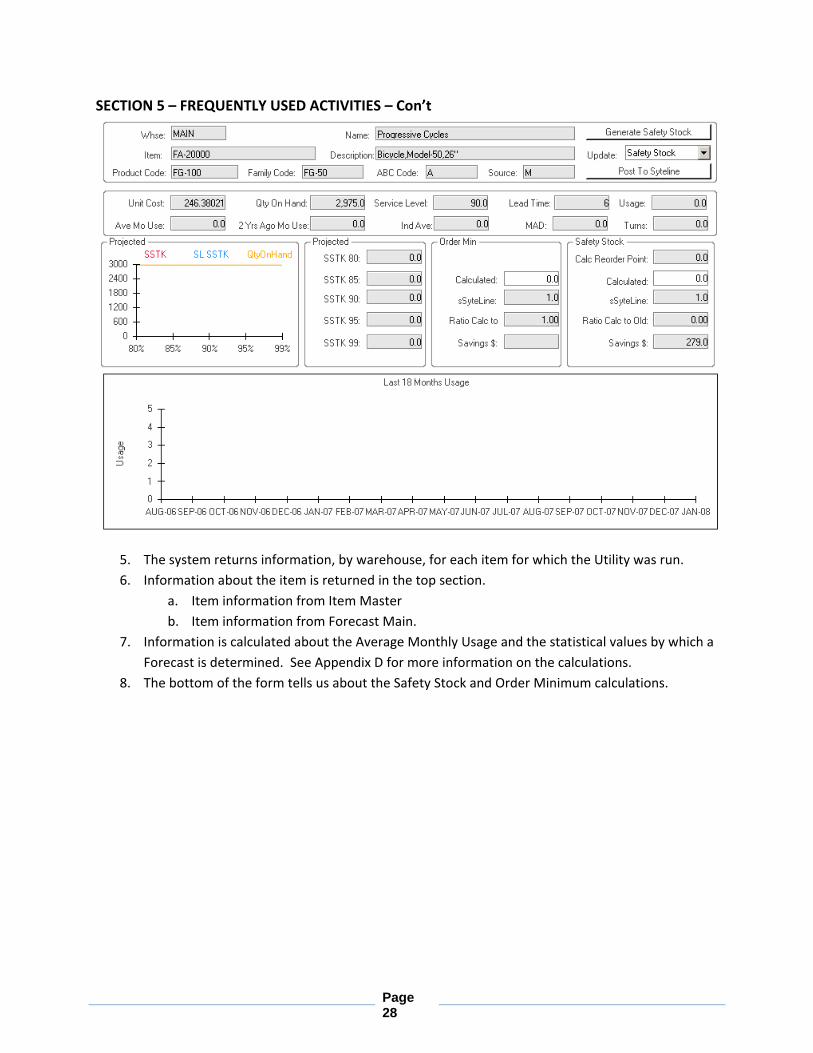
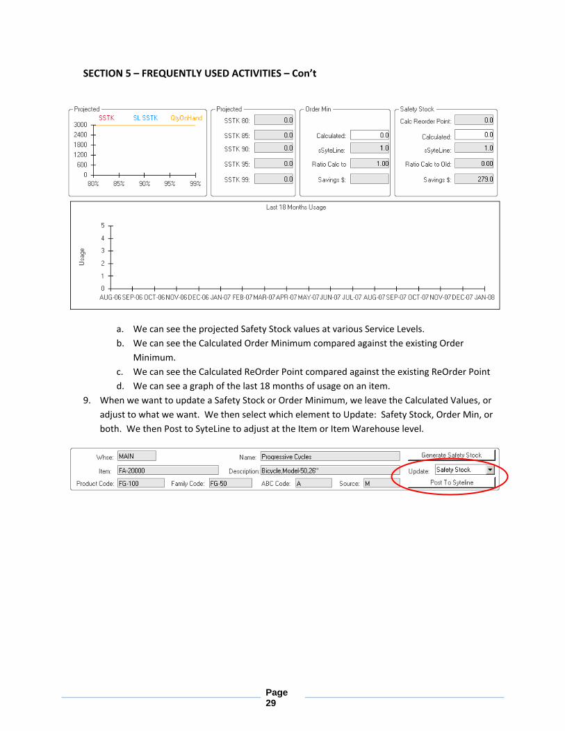
5. The system returns information, by warehouse, for each item for which the Utility was run.

6. Information about the item is returned in the top section.

a. Item information from Item Master

b. Item information from Forecast Main.

7. Information is calculated about the Average Monthly Usage and the statistical values by which a

Forecast is determined. See Appendix D for more information on the calculations.

8. The bottom of the form tells us about the Safety Stock and Order Minimum calculations.


a. We can see the projected Safety Stock values at various Service Levels.

b. We can see the Calculated Order Minimum compared against the existing Order

Minimum.

c. We can see the Calculated ReOrder Point compared against the existing ReOrder Point

d. We can see a graph of the last 18 months of usage on an item.

9. When we want to update a Safety Stock or Order Minimum, we leave the Calculated Values, or

adjust to what we want. We then select which element to Update: Safety Stock, Order Min, or

both. We then Post to SyteLine to adjust at the Item or Item Warehouse level.


Forecast-As Item Maintenance.

The Forecast As screen is accessed by right-clicking Forecast Main and is used for Forecasting Multiple items as

a single item

Some Items are very similar to other Items and it may be desirable to forecast these Items as a single Base Item. The Forecast-As feature provides this capability. The Forecast As Item must be in Forecasting and the ”Order items” must NOT be in Forecasting Items as this would double the Forecasts.

This function is also used when you wish to obsolete and item to be replaced by a newer model.

The Forecast-As Item Maintenance on the Planning Screen also allows the user to nest levels of Forecast-As Items when certain rules are followed.

Form Functionality

1. Open Forecast As form

2. Enter the Forecast As item (the item with history)

3. Enter the Order Item (the item that will be Forecast)

4. Save

5. Repeat for all like items.

Extended History

This function is used to import Legacy System Sales History for use with the Forecasting

software.

Details of use are in the System Set-up section of the manual.

Forecast Parameter Maintenance

This activity is used to maintain the system parameters that dictate how the software will

function.

Details of use are in the System Set-up section of the manual.

SECTION 6 – FREQUENTLY USED UTILITIES Auto-Calc Items Forecast

This utility is used to Update a group of items. The functionality simulates the Auto-Calc button

on the Calculations Tab. This does NOT REPLACE the functionality of the Monthly Update utility.

a. Open Form

b. Select Criteria

c. Submit

Create Initial Forecast Utility

This is actually two different forecast import utilities. One imports items based on the fact that you are selling them and the other imports items based on the fact that you are forecasting them

o Sets up Item o Collects History o Load Only Items With SyteLine Forecast – a YES here will overwrite all the information above this

entry point.

SECTION 6 – FREQUENTLY USED UTILITIES – Con’t

Field Descriptions

a. Item – SyteLine Item Number b. Product Code – SyteLine Product Code c. Planner Code – SyteLine Planner Code d. Number of Order Hits – Enter the minimum number of CO Lines the item must appear on for

the system to select the item. e. Load Items With SyteLine Forecast – This option overrides the Customer Order process and

loads all items you are presently forecasting. You may select a range of dates within which a forecast resident in SyteLine will be pulled.

f. Demand Based On – Orders/Usage – determine whether forecast will be based on order data or usage data.

g. Models to use: Default value for which model will be used during initial upload. h. Override Type: Multiplier, Replace, None are the options

i. To understand this concept please note that you will have BOTH a Forecast and an MRP input quantity. In some cases they are the same. Use the Override type to affect the MRP input (not the forecast)

ii. Multiplier – uses a 1.0 to multiply the forecast to get to MRP input iii. Replace – use an Override Value as the MRP Input for an item iv. None – System will always pass then forecast to MRP Line. There is no opportunity

to override

i. History Months – determines how much history will be used to calculate the fo Create

Initial Forecast

Forecast Monthly Utility – run monthly to update forecasts for the items specified in the ranges.


a. Select a Range of Items to run the utility against, or select the “Calculate and Update ALL

Forecasted Items” checkbox

b. Selecting the “Automatic Safety Stock” checkbox updates safety stocks for the range of

items. Exceptions, messages and items process are detailed to the User Messages form.

c. Monthly Utility will not run for items flagged inactive on the Planning Tab.

d. See the System Update Section for more details on when to run this Utility

Forecast Update MRP For All Items Utility – This utility updates the Forecast Form in SyteLine with

either the monthly or weekly forecast.

Update Review Date Utility – used to update the Review Date on a series of items. See the System

Update\Exception Messaging Section for more data on Review Dates.

SECTION 7 – ENHANCED FUNCTIONS

Planning BoM’s

Planning BoMs are typically used with it is impractical to forecast individual items; either because

the item is configured at order entry or because there are just too many permutations of the item..

A Planning BOM is established for the “parent” configuration, consisting of percentages of

“component” usage. This Parent is then forecast and passes demand to the Children. Consumption

of the forecast then takes place when a family member is added to a Sales Order. The Forecast As

form allows you to enter the family relationship where the Forecast As item is the Planning BoM and

the Order Items are the items you expect to sell.

Set-Up

1. Create a Planning Bill of Materials where you call out the percentage of each item in the

BoM.

2. SyteLine Forecasting will create a Forecast for the Planning BoM Item.

a. The Planning BoM can be created with the family members

b. Or, The Planning BoM can be created with family member components

3. As new items are configure, immediately add the Order Item to the Forecast As table tied to

the Planning BoM item.

4. Set the Update MRP Utility to run nightly.

Functionality

1. The forecast will be consumed based on the sales of one of the Order Items – based on

running the Update MRP Utility

2. A Sales Mix form will allow us to see the sales of the specific Family Members. This will help

to adjust the amount in the Planning BoM for future forecasts.

SECTION 7 – ENHANCED FUNCTIONS – Con’t

a. A Planning BoM Component Mix form will allow us to see the usage of the

components in the planning BoM. This will help us in adjusting the Planning BoM.

The Forecast Planning BoM Component Mix form allows the user to analyze a Planning

BoM where the current materials are components rather than Model numbers.

Usage Based Forecasting

Consumption of a Forecast within SyteLine, traditionally, occurs ONLY when a Sales Order is

entered for the item that is being Forecast (with the exception of Configured items).

While you could apply a Forecast to any item in the database, the consumption would only

occur if there were a Sales Order entered for that item.

Within Forecast Main, you have been able to collect Item History based on Order or Usage.

1. Order History is collected from the Sales History tables

SECTION 7 – ENHANCED FUNCTIONS – Con’t

2. Usage History is collected from Material Transaction tables and includes Sales History,

but also useage history

So, while the functionality was available to collect history and create a forecast for an item

based on its use, there was no way to consume the forecast.

SyteLine Forecasting allows for the consumption of the forecast when an item is used. Basically

the MRP Update utility looks at the material transaction table and the requirements table for

items that are being forecast and if usage is detected, the forecast is decremented by the

amount of usage, within the Look Ahead/Look Behind Parameter settings.

Forecasting in Fiscal Periods

Previously forecasting developed 12 monthly buckets of forecasted data that could be made

available to the MRP/APS engine.

SyteLine Forecasting allows the forecast periods to be aligned with the Accounting periods. So,

in addition to the traditional Monthly 4-4-5 buckets (where the weekly amount of the 5th

months’ forecast might appear lower because of the addition of the 5th week) we can bucket the

forecast in 13 periods (52 equal weeks).

To do this simply change the System Parameter to “Fiscal” periods versus “Calendar”.

The system requires 5 years of fiscal periods to be present in the Accounting Periods table. The

uses will notice a difference in the form appearance.

Now instead of 12 monthly buckets of forecast information with the column header being the

month, the form will display 13 period buckets with the column header being the Accounting

Periods.

All other functionality remain unaffected.

SECTION 8 – SYSTEM UPDATES DAILY

1. Add new items to Forecasting as conditions warrant.

The new button on the can be used to add new items.

After adding the items, go to the Calculations tab.

If the item has history, select the model that you want to use, or select Automatic Selection to have the system calculate the best-fit model.

Select Auto-Calc Fcst and the system will calculate the forecast for the next 12 months.

Review the model in the Blue Line in the Forecasting Information Section at the bottom of the screen. Or, select Forecast or History Graph to review the graph of the Model Choices Screen.

The green bar is what will be sent to MRP.

To make any adjustments to the forecast, perform group or item adjustments as detailed in Forecast Forms/Spreadsheet View/Calculations Tab/Group and Item Adjustments.

When acceptable, push the Update MRP button to populate SyteLine MRP.

If the item has no history:

Adjust the level of forecast average and select the Manual Calc Fcst button

Review the model in the Blue Line in the Forecasting Information Section at the bottom of the screen. Or, select Forecast or History Graph to review the graph of the Model Choices Screen.

The green bar is what will be sent to MRP.

To make any adjustments to the forecast, perform group or item adjustments as detailed in Forecast Forms/Spreadsheet View/Calculations Tab/Group and Item Adjustments.

When acceptable, push the Update MRP button to populate SyteLine MRP. 2. Note that items can be tracked with Forecasting without interface to MRP if desired. The "Not Forecast

With Sales" Report is a useful tool for reviewing which items are being sold regularly but are not being forecast. This report can be set to analyze data for any period of time to determine how many order lines exceeded the input target during that period of time. The text output file can be customized in a special spreadsheet format and imported back to load the new items. Another way to add new items is to use the Create Initial Forecasts at Installation Utility from the Forecasted Items Screen.

3. View the Message Log File for recommended changes by choosing User Messages off of the File Menu.

MONTHLY

1. As early every month as possible, but after all new orders and shipments have been processed for the preceding month (usually on the 2nd or 3rd workday), run the Forecast Monthly Utility .

2. Run the Forecast Update MRP for All Items Utility from the Utilities menu. This will update SyteLine’s forecasting form with new data for all items – that do not have an exception situation.

3. Review Exceptions and make and necessary Forecast changes. This can be done by either using the filter for exceptions only from the spreadsheet view in Forecasted Main Form or by running the Exceptions Report.

4. Run the Export/Update Safety Stocks/Order Min Utility from the Utilities Menu under the Forecasting tab in the Explorer. Don't update directly from this utility. After reviewing and changing the data, use the Import Safety Stock and Order Min to SyteLine Utility on the Utilities menu. Please be sure you understand the difference between the Safety Stock and the Variable Safety Stock before you upload data from these calculations.

SECTION 8 – SYSTEM UPDATES – Con’t

AS REQUIRED

1. Use the Marketing Screen options to analyze data and determine overall trends in the market place.

2. Use the Forecast Items Not Forecast With Sales Report to determine new items to add to Forecasting.

EXCEPTION MESSAGING A part of the Monthly Utility is the creation of exceptions messages. These messages occur when a pre-

determined threshold has been met.

Exception Messages can be encountered in one of three ways:

1. Review Date – this is used when adding a new item or when making major changes to an item

a. Navigate to the Planning Tab

b. Set a Review Date

c. When the system reaches the Review Date an exception is created

2. D=Demand Spike – you control the size of the reference point. The spike must exceed your demand filter before this condition occurs

3. T=Forecast not Tracking with actual – again – you decide the amount of tracking error you will

tolerate.

See Appendix on “Demand Filter and Track Limit” for more information.

SECTION 9 – FREQUENTLY USED REPORT

All Forecasting reports will open as an Excel document. They can be modified, printed and saved as .xls,

.csv or .txt.

Forecast As Items Report

Shows the relationship between Forecast As items.

Calculate Best Fit Models Report

Performs a series of calculations and suggests Model changes by item, where needed.

Consumption Exception Report

Allows a "real time" review of forecasts and their consumption by customer orders. Early action can be taken on those items not tracking to their forecasts.

Detail Forecast Report

Shows detail information. One item number is printed per page.

Exceptions Report

Show forecast items with exceptions. Prints in summary report format.

Not Forecast with Sales Report

Shows items being sold but not forecast and facilitates analysis for a period of time for items that are being sold but are not being forecast. A filter can be applied for the number of customer order lines so that items with only a few lines can be suppressed. These items should be reviewed to determine if they should be forecast.

Value of Standard Groups Report

The report is actually several reports that can be run simply be changing the "No" to "Yes" for each report. Any "From" and "To" limits entered will be used for all of the reports that are selected. Useful for understanding the impact of a forecast.

Customer Not Forecast Report

Used to evaluate items that are not forecasted but do have Customer Orders to determine if that Item should be forecasted

Group Memberships Report

Used to evaluate group memberships

APPENDIX A – Forecasting Models

MODEL TYPES

D - Display History Only

1. This model is used to accumulate and display demand history for informational purposes without doing any forecasting.

M - Moving Average for Number of Months

1. The moving average model calculates the forecast using an average of a number of most recent months’ data. The number of months field determines how many months of data will be used for the moving average. Each month a month is dropped and a new month of data is added.

2. The advantage of this model is that it is both simple and represents the most recent data. 3. The disadvantage is that if a high sales month is dropped and a low sales month is added (or vice

versa) there can be a substantial change in the forecast.

H - Horizontal (Exponential Smoothing)

1. The horizontal model uses a weighting factor (alpha factor) to give that factor’s share or weighting to the current month demand. The old forecast is weighted by one minus that factor. This if the alpha factor (or weighting factor) is 0.1, then 10% weight will be given to the current month demand and 90% weight would be given to the old forecast.

2. For example: Alpha Factor = 0.1 Old Forecast = 100 Current Demand = 140 New Forecast = (0.1 * 140) + (0.9 * 100) = 14 + 90 = 104

3. Exponential Smoothing has the advantage of smoothing demand fluctuations and does not require the maintenance of historical data to use. The calculations are simple if forecasting is being done manually.

4. An alpha factor of 0.1 approximates a 19 month moving average and would be appropriate for stable products. Higher alpha factors should be used for faster response. Generally an alpha factor greater than 0.3 should not be used.

5. Exponential Smoothing gets its name from the shape of the curve formed by the weight impact of previous demand periods.

6. See the Alpha Factors table for the relative weighting of alpha factors of 0.1 to 0.4.

L - Lumpy Model - D637 (Demand has several zero periods each year)

1. The Lumpy Model is the same as the Horizontal Model but uses a very low alpha factor (usually 0.05). Consequently this model changes very slowly.

2. Monthly data may come in as 0, 0, 0, 37, 0, 0, 3 and be smoothed by this model. If the demand is unreasonable it will not be used. If the demand is consistently higher or lower than the forecast then an exception condition (Forecast Not Tracking) will occur.

3. Usually the initial Forecast average will be determined by management policy for this type of item depending on the customers, normal order sizes, and importance of quick deliveries for this kind of

item. A Forecast override replacing the Forecast will frequently be used. The Forecast will then simply be a tracking and exception condition vehicle.

4. A custom lumpy model that analyzes order size is available for those who are interested. This model can be customized to meet any unique requirements. There is no charge for this model.

T - Trend Model (Demand is increasing or decreasing)

1. Trend models can be dangerous to use if not properly understood and managed. Since they are based on either history or management expectations and are either increasing or decreasing forecast levels, the actual demand data may be rapidly changing direction without the model being able to adapt quickly enough (or too quickly in some situations).

2. The trend model consists of a beginning point (Forecast Average) and a trend (slope) value. The Trend Value is the monthly quantity increase or decrease (minus) in the average.

3. After the initialization process this model will use exponential smoothing to update the model’s variables each month in order to stabilize fluctuations.

S - Seasonal Model (Demand has seasonal patterns)

1. The Seasonal model is used when data exhibits a seasonal pattern year after year. For example calendar sales are high late in the year and early in the year and low the rest of the year. This model can be dangerous if seasonality is not consistent. It should not be used unless market conditions are thoroughly understood.

2. This model uses the Base Index values as multipliers to adjust the Forecast Average for seasonality each month.

3. After initialization, exponential smoothing is used to update these values each month.

B - Trend Seasonal Model (Demand has Trend and is Seasonal)

1. This model combines the features of both the Trend and Seasonal models. Consequently it is also the most dangerous to use. Using the calendar example, if sales are expected to increase by 10% a month due to new contracts with new clients then this model may be appropriate.

2. This model uses both the Trend Value and Base Index Values to adjust the Forecast Average. 3. After initialization, exponential smoothing is used to update these values each month.

C - Customer Supplied Model

1. This model uses the Customer Supplied Forecast. 2. This model does not use values to adjust the Forecast Average, it is the sum of what has been

supplied by the Customer.

R - Roll-Up Model

1. This model uses the Roll-Up Forecast. This model works the same as the Customer Supplied Model except the Customer# in the Customer#/Item combination is replaced by one of the chosen variables for Model R (Warehouse, Salesman, Sales Class, Customer Type and End User Type).

2. This model also does not use values to adjust the Forecast Average, it is the sum of what has been supplied by the Customer.

ALPHA FACTORS

The Alpha Factor is the Weighting Factor used to weight the Old Forecast and New Data Month. This factor usually

varies between .05 (5% weight and .20 (20% weight) to New Data.

Period 0.1 0.2 0.3 0.4

-1 0.100 0.200 0.300 0.400

-2 0.090 0.160 0.210 0.240

-3 0.081 0.128 0.147 0.144

-4 0.073 0.102 0.103 0.086

-5 0.066 0.082 0.072 0.052

-6 0.059 0.066 0.050 0.031

-7 0.053 0.052 0.035 0.019

-8 0.048 0.042 0.025 0.011

-9 0.043 0.034 0.017 0.007

-10 0.039 0.027 0.012 0.004

-11 0.035 0.021 0.008 0.002

-12 0.031 0.017 0.006 0.001

-13 0.028 0.014 0.004 0.001

-14 0.025 0.011 0.003 0.001

-15 0.023 0.009 0.002 0.000

-16 0.021 0.007 0.001 0.000

Total 0.815 0.972 0.997 1.000

For an alpha factor of 0.1 note that the current period (-1) has a 10% impact and 2 months ago a 9% impact and

three months ago has an 8.1% impact.

Number of Months to Reach 80%

Months 16 8 5 3

Total 0.815 0.832 0.832 0.870

Note that the 0.4 factor gives 40% weight to the first previous month, then 24% weight to the second previous

month, then 14.4% weight to the third previous month for a total of 78.4% weight to these three months. 0.4 is

not recommended since the forecast would fluctuate too much month to month as the new month received 40%

weight.

APPENDIX B – Forecasting FAQ’s

Who do I contact for support?

Business Technology Associates, Austin TX

(512)343-9600

www.btasystems.com

What is the typical business process for using Forecasting?

1) Run “Create Initial Forecasts” (to create the Forecast Masters for all new items)

2) Run “Forecast Calculation” (After closing the previous month inventory and shipping…., this extracts the history

for the previous month(s) and calculates the forecasts for all items)

3) Graph and analyze item forecasts individually or in groups in the History Screen… make override adjustments for

special events or other considerations. (Item overrides and group overrides)

4) Run “MRP Input for All Forecasted Items” (this updates the forecasts in the MRP\APS system)

5) Run “Export\Update” Safety Stocks\Order Mins (this calculates the values and creates a spreadsheet for review,

after review the spreadsheet is imported to update the item masters)

6) Weekly review the Exceptions on the main screen and make revisions to the individual forecasts… these can be

applied to MRP\APS individually by clicking “Update MRP” in the item’s planning screen.

Does SL Forecasting support multi currency?

When sales history is gathered on a dollar basis, the currency is translated. (if there is a customer order exchange

rate then that rate is applied).

Any screen that displays dollar values will display in the same currency as the site\db the order was entered."

Does SL Forecasting support SyteLine multi-site functionality?

A separate Forecast database is required for each SyteLine site. Forecasts are done for each site\db separately and

loaded into the MRP forecast for each site separately. Customization is possible to consolidate all sites into a

single forecast database and rules must be designed on how to allocate the generated forecast back to each site.

How does forecasting handle consumption of the forecast?

Forecasting allows SyteLine to handle all consumption. If components are forecasted, we recommend that SyteLine time fences be used to determine when the forecast and when actual demand take control.

For companies that make mostly custom products (do not have standard sellable catalogue items or standard

BOM’s), how does SL Forecasting help their material planning.

SL Forecasting can forecast sellable items or components. For each forecasted item you specify whether history is based on just sales or on total usage. If you specify usage, a forecast is created based on the material issues of the item (from your material transactions file) and this creates a forecast for the component, which then drives MRP\APS. Component forecasts are not consumed by customer orders (since there is no customer order for the components)… therefore, a time fence concept must be used to control whether the forecast or the actual demand drives MRP\APS. This can be accomplished with the Override and Over Type on the forecast variables screen. For instance, a company could set a “Time-Phased” override for the first month out of “0”. This would result in actual demand driving the current month, and the forecast driving demand after that. The safety stock calculation, which considers average usage and lead time, will handle the variations that might occur during the current month to prevent any stock outs. Forecasting also has a new feature that will consume the forecast based on material issues rather than customer orders… please call BTA for help with understanding this.

How customizable is Forecasting and what enhancements are planned?

BTA is very open to customizing to a client’s needs and building in new functionality to future versions.

Forecasting source code is available for purchase by the customer.

What Implementation and training services are recommended?

Three days on site for Install, train, and minor business process consulting. The program is easy to install and use… a quick start implementation can be accomplished with 1 day of Classroom training (Texas) and self installation.

Is there a way to forecast by group instead of generating individual forecasts?

There are three methods to forecast families or groups of items:

1) Automatically calculate all the item forecasts then adjust by group:

SyteLine Forecasting can create the forecasting master records in mass by specifying a range of product codes or

item numbers, etc. (Create Initial Forecasts Activity). Then you calculate forecasts for all items at once by simply

clicking the Monthly Forecast Calculation. This analyzes historical usage, applies the previously specified statistical

model, and calculates individual forecasts for every item. You can then graph these forecasts by various groupings

and adjust all the items in any grouping by applying a percentage increase or decrease to the entire group (Group

Memberships Activity). The adjusted forecasts are then loaded into the MRP\APS plan in mass by clicking "MRP

Input for all Forecasted Items".

2) Planning bills:

Setup a planning bill in SyteLine then use the SyteLine Forecasting "Re-calculate Planning BOM Percent Factors".

This looks at history and calculates what percent of the time each option was selected and gives you the option to

set the planning bill percentages to the historical percentages, or enter an override percentage.

3) Forecast a user defined Group

Create a group tied to a specific product code. Then create forecast for the group, which in turn creates individual

forecasts in SyteLine for each member of the group based on their relative usage history (which can be adjusted)

This feature is not in the current version for SyteLine 7… call if you have a customer requesting it.

How is the Safety Stock (reorder point) calculated?

It uses the APICS approach, which calculates the value considering the variability of demand during the lead, the

desired service level (forecasting parameter) and the lead-time.

How is the Order Min (lot size) calculated?

The formula used Order Minimum = square root ((2AS)/(IC)) where A = Annual Usage S = Setup Cost (See Below) I = Cost of Carry Inventory (Forecast Parameter) C = Item’s Current Unit Cost The Setup Cost for Purchased items is a Forecast Parameter. The Setup Cost for Manufactured items is the SyteLine setup cost for the item plus the Forecast Parameter for additional job setup cost.

Definitions:

Status… item status (ie inactive)

Safety stock... you specify service level % and It looks at lead time variability

Order min… considers setup cost and carry cost

Bi values… base index.. to adjust for seasonal factors (December is 1.8 x the average)

Appendix C – Demand Filter and Track Limit

Demand Filter - This value is used to determine an unreasonable demand exception, and usually

will range from 4 to 6. A lower value is more sensitive (will consider lesser demands as

unreasonable) and a higher level is less sensitive. A month’s demand is considered unreasonable

if the demand exceeds the forecast average by more the product of the demand filter value and

the average forecast error (Mean Absolute Deviation).

Un

it V

olu

me

Forecast Interval

Unreasonable Demand

Upper Limit

Lower Limit

FCST

ACTUAL

Track Limit - Tracking Signal Limit. This value is used together with the Tracking Signal Value

to determine a Forecast Tracking Signal Exception. The less the value, the sooner an exception

condition will occur. 6 is a typical value used for this purpose. If the item is a new product and

the Forecast is to be monitored closely then a smaller value would be used.

Track Value - Tracking Signal Value. Calculated equal to the Sum of Errors divided by the

Average Error. When being compared to the Tracking Signal Limit, the sign is ignored.

Resetting the Sum of Errors resets the Tracking Signal Value.

Tracking Example: The sum of the errors is –64. We have accumulated an error of -64 since the last time

we this item was manually updated. The sum of the errors divided by the average error is -7.0. Which is

greater than 6 (the tracking limit). Therefore the Exception condition of Tracking is generated.

Un

it V

olu

me

Forecast Interval

Tracking Error

Upper Limit

Lower Limit

FCST

ACTUAL

APPENDIX D – Safety Stock and Order Min Calculations Safety Stock Calculation 1. The latest 2 years (counting back from “yesterday”) of matltran job issues and shipments are retrieved. The oldest year is averaged and the average is used only for display reference. 2. The Average and MAD (Mean Absolute Deviation) are calculated for the latest year. If any month has more than 80% of the demand for the year is dropped for calculations but left in history and totals. 3. Set Service Level to:

1. Forecast Item’s Service Level if not zero or 2. Forecasting Parameter service Level if not zero or 3. 80% if both of the above are zero.

4. Look up the Service Factor in a table for the given service level. This is a statistical table of standard deviations and probability percent. (e.g. 95% Service Level has a service factor of 1.96 Standard Deviations). 5. Compute Safety Stock for one month by multiplying the Service Factor Times the MAD times 1.25 (1.25 MAD’s = 1 Standard Deviation). The MAD must not exceed the Average or the Average is used. This corrects for certain unusual demand distributions. 6. Adjust Safety Stock if the lead time is greater than one month. If the lead time is zero use 1 month for Purchased items and 0.5 months for Manufactured items. Otherwise use the lead time. If the lead time is greater than 1 month then multiply the safety stock by the square root of the lead time in months. This is to compensate for not calculating the MAD and Average based on time periods that are a multiple of the lead time. In other words the safety stock for three months is less than three times the safety stock for one month. Data could be grouped in lead time intervals but one month is the usual time frame looked at and this approximation is easier for the user to understand and produces a more consistent result in the real world. 7. If the Safety Stock is less and 1 and at least 0.35 then the Safety Stock is set to 1. 8. The Reorder Quantity is the Monthly Average times the lead time plus the Variable Safety Stock. (Demand over lead time plus safety stock). 9. If the Reorder Quantity is Greater Than that of the default warehouse and the number of hits in 12 months is only 1 then the new reorder quantity is set to the old one and the variable safety stock is set to zero. Order Mininum Calculation 1. The formula used is Order Minimum = square root ((2AS)/(IC)) where

A = Annual Usage S = Setup Cost (See Below) I = Cost of Carry Inventory (Forecast Parameter) C = Item’s Current Unit Cost

The Setup Cost for Purchased items is a Forecast Parameter. The Setup Cost for Manufactured items is the Syteline setup cost for the item plus the Forecast Parameter for additional job setup cost.

2. The calculation is restricted to a minimum 1 month supply and maximum 6 month supply. If there is only 1 hit in the history then the new order minimum is set to zero. NOTE: These calculations are a guide to help users review their safety stocks and lot sizes. Great care should be used since a major cause of excess and obsolete inventory is improperly used safety stocks and lot sizes. This is especially true in a multi-level MRP environment where safety stocks and order minimums must be restricted to only the appropriate items and never use on all items.

SyteLine Forecasting System Implementation Guide V8 · Page 1 SyteLine Forecasting System...

Documents

Transcript of SyteLine Forecasting System Implementation Guide V8 · Page 1 SyteLine Forecasting System...