Systolic, Transposed & Semi-Parallel Architectures and Programming
14
Abstract The critical routines within signal processing algorithms are typically data intensive and iterate many times, carrying out the same functions on multi-dimensional arrays and input streams. These routines use the vast majority of an implementation’s resources, and for the longest time over the course of the algorithms execution. Such routines are classed as Nested-Loop Programs. Whether the implementation is software running on a processor or a higher performance customized hardware implementation, there is always a tradeoff between the throughput performance (execution-time) and the resources used such as the amount of processor memory and registers in a software implementation or the gate-count in a hardware implementation. This article shows the reader techniques and methods for manipulating a signal processing algorithm, in particular those conforming to a Nested-Loop Program, and the different generic implementation architectures along this tradeoff spectrum, as well as the different methods for describing and analyzing an algorithm implementation. Each of these methods for describing an algorithm is shown to correspond to a different abstraction-level view and as such exposes different features and properties for ease of analysis and manipulation. Manipulation techniques, mainly algorithmic- transformations are described and it is shown how these transformations take an implementation and form a new one at a different point in the trade-off spectrum of resources used versus throughput by performing calculations in a different order and a different way to arrive at the same result. Contents 1 Loop Optimization 1.1 The Unrolling Transformation 1.2 The Skewing Transformation 2 The three abstraction levels for representing Signal Processing Algorithms 2.1 Code Representation 2.2 Data-dependency Graph 2.3 Hardware Implementation 3 Parallel implementations of a Signal Processing algorithm 3.1 The Transposed FIR Filter 3.2 The Systolic FIR Filter 3.3 The Semi-Parallel FIR Filter Conclusion Systolic, Transposed & Semi-Parallel Architectures and Programming Sandip Jassar http://www.linkedin.com/in/sandipjassar
-
Upload
sandip-jassar-sandipjassarhotmailcom -
Category
Technology
-
view
755 -
download
0
Transcript of Systolic, Transposed & Semi-Parallel Architectures and Programming
Abstract
The critical routines within signal processing algorithms are typically data intensive and
iterate many times, carrying out the same functions on multi-dimensional arrays and input streams. These routines use the vast majority of an implementation’s resources, and for the longest time over the course of the algorithms execution. Such routines are classed as
Nested-Loop Programs. Whether the implementation is software running on a processor or
a higher performance customized hardware implementation, there is always a tradeoff
between the throughput performance (execution-time) and the resources used such as the
amount of processor memory and registers in a software implementation or the gate-count in a hardware implementation. This article shows the reader techniques and methods for manipulating a signal processing algorithm, in particular those conforming to a Nested-Loop Program, and the different generic implementation architectures along this tradeoff spectrum, as well as the different methods for describing and analyzing an algorithm implementation. Each of these methods for describing an algorithm is shown to correspond
to a different abstraction-level view and as such exposes different features and properties for
ease of analysis and manipulation. Manipulation techniques, mainly algorithmic-
transformations are described and it is shown how these transformations take an
implementation and form a new one at a different point in the trade-off spectrum of resources used versus throughput by performing calculations in a different order and a different way to arrive at the same result.
Contents
1 Loop Optimization
1.1 The Unrolling Transformation
1.2 The Skewing Transformation
2 The three abstraction levels for representing Signal Processing Algorithms 2.1 Code Representation
2.2 Data-dependency Graph
2.3 Hardware Implementation
3 Parallel implementations of a Signal Processing algorithm
3.1 The Transposed FIR Filter 3.2 The Systolic FIR Filter 3.3 The Semi-Parallel FIR Filter
Conclusion
Systolic, Transposed & Semi-Parallel
Architectures and Programming
Sandip Jassar
http://www.linkedin.com/in/sandipjassar
1 Loop Optimization
The Nested-Loop Program (NLP) form of a signal processing algorithm represents what’s
known as its sequential model of computation. The Finite Impulse Response (FIR) filter is the
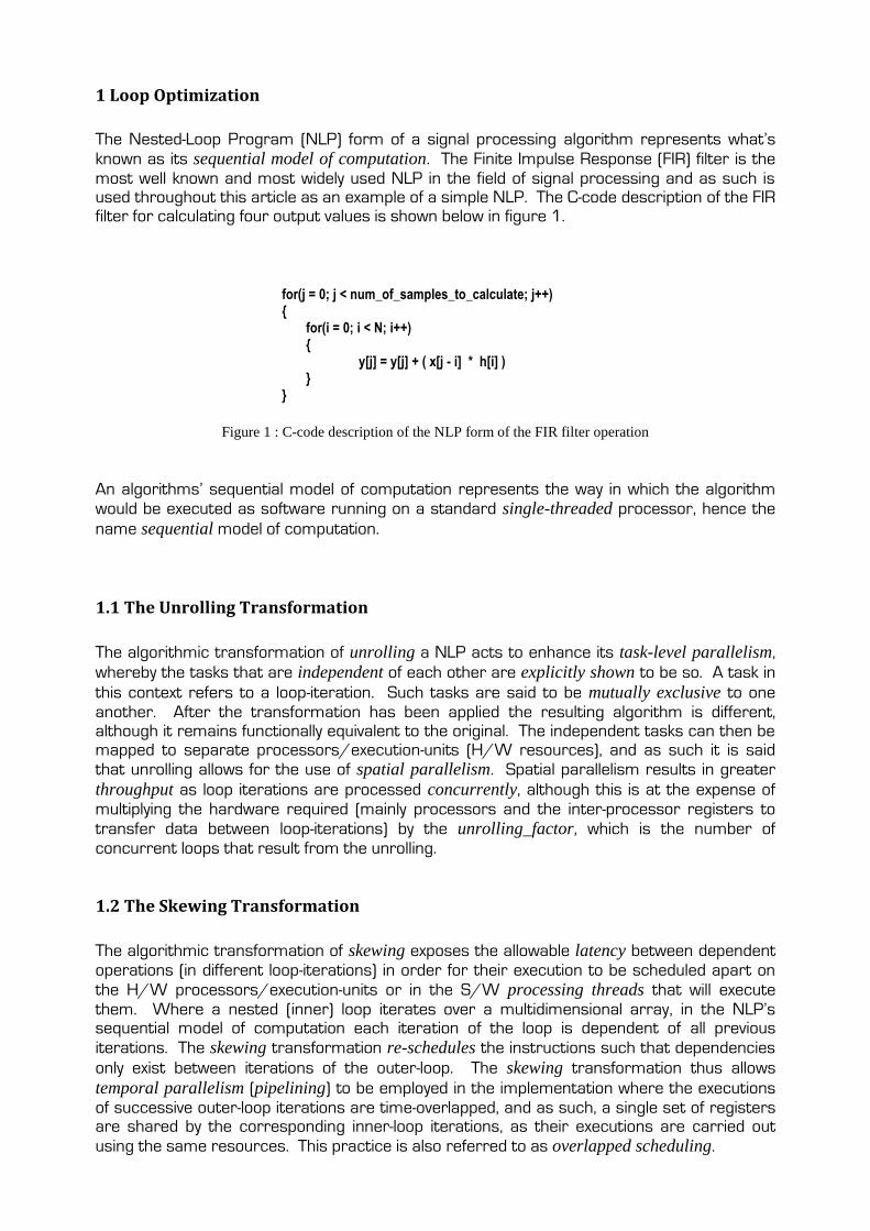
most well known and most widely used NLP in the field of signal processing and as such is used throughout this article as an example of a simple NLP. The C-code description of the FIR filter for calculating four output values is shown below in figure 1.
for(j = 0; j < num_of_samples_to_calculate; j++) { for(i = 0; i < N; i++) { y[j] = y[j] + ( x[j - i] * h[i] ) } }
Figure 1 : C-code description of the NLP form of the FIR filter operation
An algorithms’ sequential model of computation represents the way in which the algorithm
would be executed as software running on a standard single-threaded processor, hence the
name sequential model of computation.
1.1 The Unrolling Transformation
The algorithmic transformation of unrolling a NLP acts to enhance its task-level parallelism,
whereby the tasks that are independent of each other are explicitly shown to be so. A task in
this context refers to a loop-iteration. Such tasks are said to be mutually exclusive to one
another. After the transformation has been applied the resulting algorithm is different, although it remains functionally equivalent to the original. The independent tasks can then be mapped to separate processors/execution-units (H/W resources), and as such it is said
that unrolling allows for the use of spatial parallelism. Spatial parallelism results in greater
throughput as loop iterations are processed concurrently, although this is at the expense of
multiplying the hardware required (mainly processors and the inter-processor registers to
transfer data between loop-iterations) by the unrolling_factor, which is the number of
concurrent loops that result from the unrolling.
1.2 The Skewing Transformation
The algorithmic transformation of skewing exposes the allowable latency between dependent
operations (in different loop-iterations) in order for their execution to be scheduled apart on
the H/W processors/execution-units or in the S/W processing threads that will execute
them. Where a nested (inner) loop iterates over a multidimensional array, in the NLP’s sequential model of computation each iteration of the loop is dependent of all previous
iterations. The skewing transformation re-schedules the instructions such that dependencies
only exist between iterations of the outer-loop. The skewing transformation thus allows
temporal parallelism (pipelining) to be employed in the implementation where the executions
of successive outer-loop iterations are time-overlapped, and as such, a single set of registers are shared by the corresponding inner-loop iterations, as their executions are carried out
using the same resources. This practice is also referred to as overlapped scheduling.
Overall the unrolling and skewing transformations can be used to transform a sequential
model of computation into something that it is closer to a data-flow model which exploits the
algorithm’s inherent parallelism and thus can be used to yield a more efficient implementation. Dependent operations can also be scheduled apart by simply changing the order in with operations are executed. The simplest example of this is when the inner and outer loop indices are swapped.
2 The three abstraction levels for representing Signal Processing Algorithms
The following section shows how to represent a signal processing algorithm in terms of its
Code description, as a Data-dependency graph and its Hardware implementation. Code shows
how an algorithm would be executed on a processor (its Software implementation) and is used
to describe the algorithm from the highest abstraction level. The Hardware implementation
represents the lowest abstraction level. The reader will learn how to transfer the description
of an algorithm between these abstraction levels, and also gain an appreciation of which characteristics of an algorithm are greater exposed for ease of manipulation at a particular abstraction level. The example algorithm used throughout this section is the FIR (Finite Impulse Response) filter in its basic sequential form, as the FIR filter is very simple and widely used in the field of signal processing.
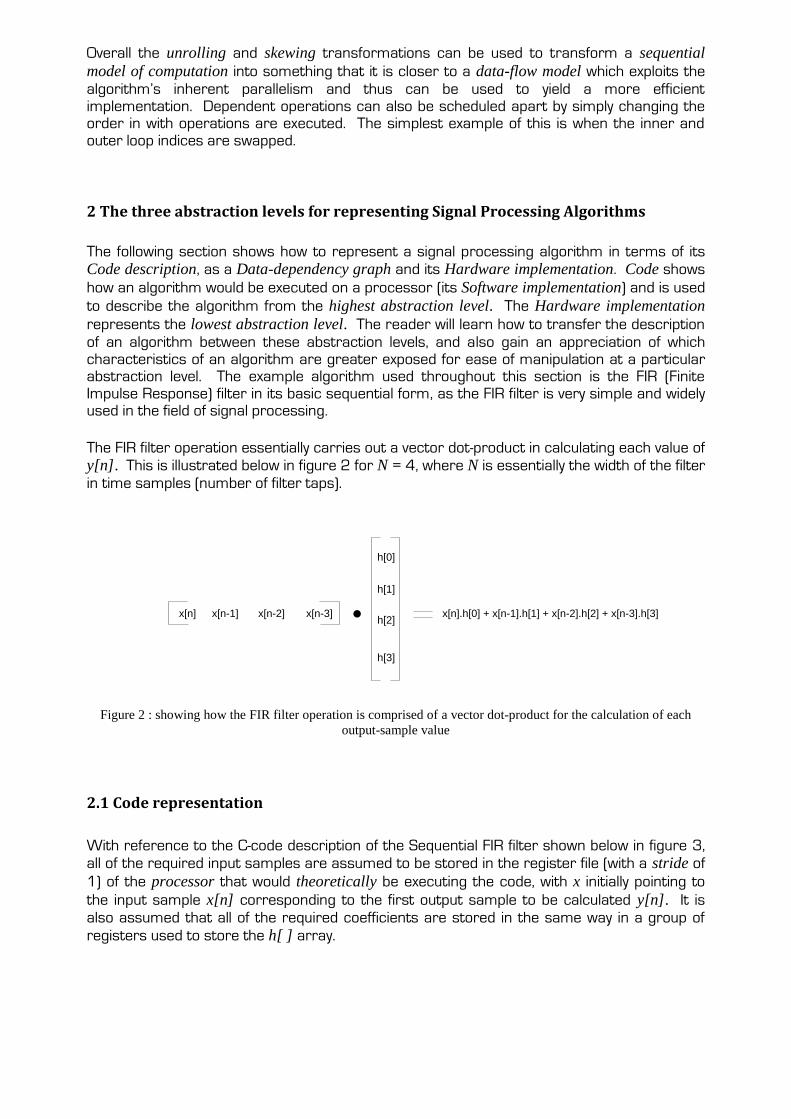
The FIR filter operation essentially carries out a vector dot-product in calculating each value of
y[n]. This is illustrated below in figure 2 for N = 4, where N is essentially the width of the filter
in time samples (number of filter taps).
x[n] x[n-3]x[n-2]x[n-1]
h[0]
h[1]
h[2]
h[3]
x[n].h[0] + x[n-1].h[1] + x[n-2].h[2] + x[n-3].h[3]
Figure 2 : showing how the FIR filter operation is comprised of a vector dot-product for the calculation of each
output-sample value
2.1 Code representation
With reference to the C-code description of the Sequential FIR filter shown below in figure 3,
all of the required input samples are assumed to be stored in the register file (with a stride of
1) of the processor that would theoretically be executing the code, with x initially pointing to
the input sample x[n] corresponding to the first output sample to be calculated y[n]. It is
also assumed that all of the required coefficients are stored in the same way in a group of
registers used to store the h[ ] array.
void sequentialFirFilter( int num_taps, int num_samples, float *x, const float *h[ ], float *y )
{
int i, j; // ‘j’ is the outer-loop counter and ‘i’ is the inner-loop index
float y_accum; // output sample is accumulated into ‘y_accum’
float *k; // pointer to the required input sample
for( j = 0; j < num_samples; j++ )
{
k = x++; // x points to x[n+j] and is incremented (post assignment) to point to // x[(n+j)+1]
y_accum = 0.0;
for( i = 0; i < num_taps; i++ )
{
y_accum += h[i] * *(k--); // y[n+j] += h[i] * x[(n+j) - i]
}
*y++ = y_accum; // y points to the variable address where y[n+j] is to be written and is // incremented (post assignment) to point to the variable address
} // where the next output sample y[(n+j)+1] is to be written
}
Figure 3 : A C-code description of the FIR filter’s sequential model of computation
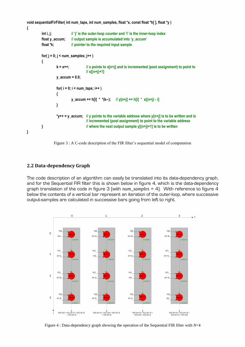
2.2 Data-dependency Graph
The code description of an algorithm can easily be translated into its data-dependency graph, and for the Sequential FIR filter this is shown below in figure 4, which is the data-dependency
graph translation of the code in figure 3 (with num_samples = 4). With reference to figure 4
below the contents of a vertical bar represent an iteration of the outer-loop, where successive output-samples are calculated in successive bars going from left to right.
h(0)
h(1)
h(2)
x[n]
+
h(3)
h(0).x[n] + h(1).x[n-1] + h(2).x[n-2]
+ h(3).x[n-3]
+
+
x[n-1]
x[n-2]
x[n-3]
h(0)
h(1)
h(2)
x[n+1]
+
h(3)
h(0).x[n+1] + h(1).x[n] + h(2).x[n-1]
+ h(3).x[n-2]
+
+
x[n]
x[n-1]
x[n-2]
h(0)
h(1)
h(2)
x[n+2]
+
h(3)
h(0).x[n+2] + h(1).x[n+1] +
h(2).x[n] + h(3).x[n-1]
+
+
x[n+1]
x[n]
x[n-1]
h(0)
h(1)
h(2)
x[n+3]
+
h(3)
h(0).x[n+3] + h(1).x[n+2] +
h(2).x[n+1] + h(3).x[n]
+
+
x[n+2]
x[n+1]
x[n]
j
i
MACC_1
MACC_1
MACC_1
MACC_1
MACC_1
MACC_1
MACC_1
MACC_1
MACC_1
MACC_1
MACC_1
MACC_1
MACC_1
MACC_1
MACC_1
MACC_1
y-accum
y-accum
y-accum
y-accum
y-accum
y-accum
y-accum
y-accum
y-accum
y-accum
y-accum
y-accum
y-accum
y-accum
y-accum
y-accum
0 1 2 3
0
1
2
3
Figure 4 : Data-dependency graph showing the operation of the Sequential FIR filter with N=4
The circles in each bar of figure 4 above represent the instances of the physical operators that carry out each iteration of the inner-loop, where successive iterations are represented from top to bottom. The name given to this physical operator for the Sequential FIR filter is
MACC_1 as a multiply-accumulate is the only instruction (in S/W) or operation (in H/W) that
is carried out, and with the FIR filter’s sequential model of computation all instructions/operations in the inner-loop are dependent on all of the previous ones, and the outer-loop is carried out one iteration at a time, so only one instruction/operation can be
scheduled for execution at any one time and thus only one execution-unit can be used.
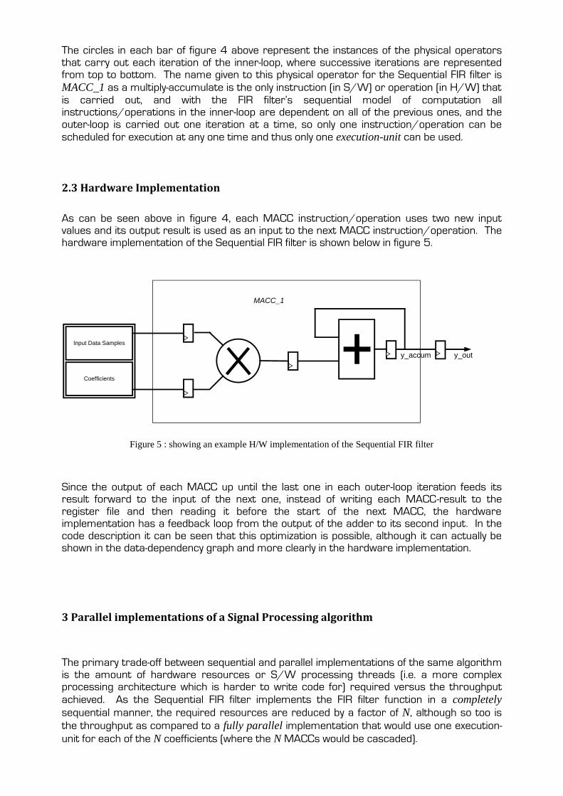
2.3 Hardware Implementation
As can be seen above in figure 4, each MACC instruction/operation uses two new input values and its output result is used as an input to the next MACC instruction/operation. The hardware implementation of the Sequential FIR filter is shown below in figure 5.
MACC_1
y_out
Input Data Samples
Coefficients
y_accum
Figure 5 : showing an example H/W implementation of the Sequential FIR filter
Since the output of each MACC up until the last one in each outer-loop iteration feeds its result forward to the input of the next one, instead of writing each MACC-result to the register file and then reading it before the start of the next MACC, the hardware implementation has a feedback loop from the output of the adder to its second input. In the code description it can be seen that this optimization is possible, although it can actually be shown in the data-dependency graph and more clearly in the hardware implementation.
3 Parallel implementations of a Signal Processing algorithm
The primary trade-off between sequential and parallel implementations of the same algorithm is the amount of hardware resources or S/W processing threads (i.e. a more complex processing architecture which is harder to write code for) required versus the throughput
achieved. As the Sequential FIR filter implements the FIR filter function in a completely
sequential manner, the required resources are reduced by a factor of N, although so too is
the throughput as compared to a fully parallel implementation that would use one execution-
unit for each of the N coefficients (where the N MACCs would be cascaded).
As can be seen from figure 3 above, and more clearly from the data-dependency graph (shown above in figure 4), the Sequential FIR filter evaluates (accumulates) only one output
value at a time. Assuming that each multiplication of x[(n+j)-i] and h[i] takes one clock cycle,
then the performance of this implementation is given by the following equation:
Throughput = Clock frequency ÷ Number of coefficients
The simplest fully-parallel FIR filter implementation is the Direct form type 1. This is formed by
completely unrolling the inner-loop and mapping each of the unrolled instructions/operations to separate execution-units. The problem with this implementation is that the outputs of the execution-units (MACC outputs) are all summed through an adder-chain, where the resulting latency (and gate-count with a H/W implementation) mean that the Direct form type 1 FIR
filter does not scale very well for large problem sizes (N). The other reason why the Direct
form type 1 FIR filter is not used in signal processing is that it requires N input values to be read in for each output value to be calculated, and this design feature does not scale very well for large N due to the greater latency and possibly (depending on the implementation) the higher number of memory read ports.
3.1 The Transposed FIR filter
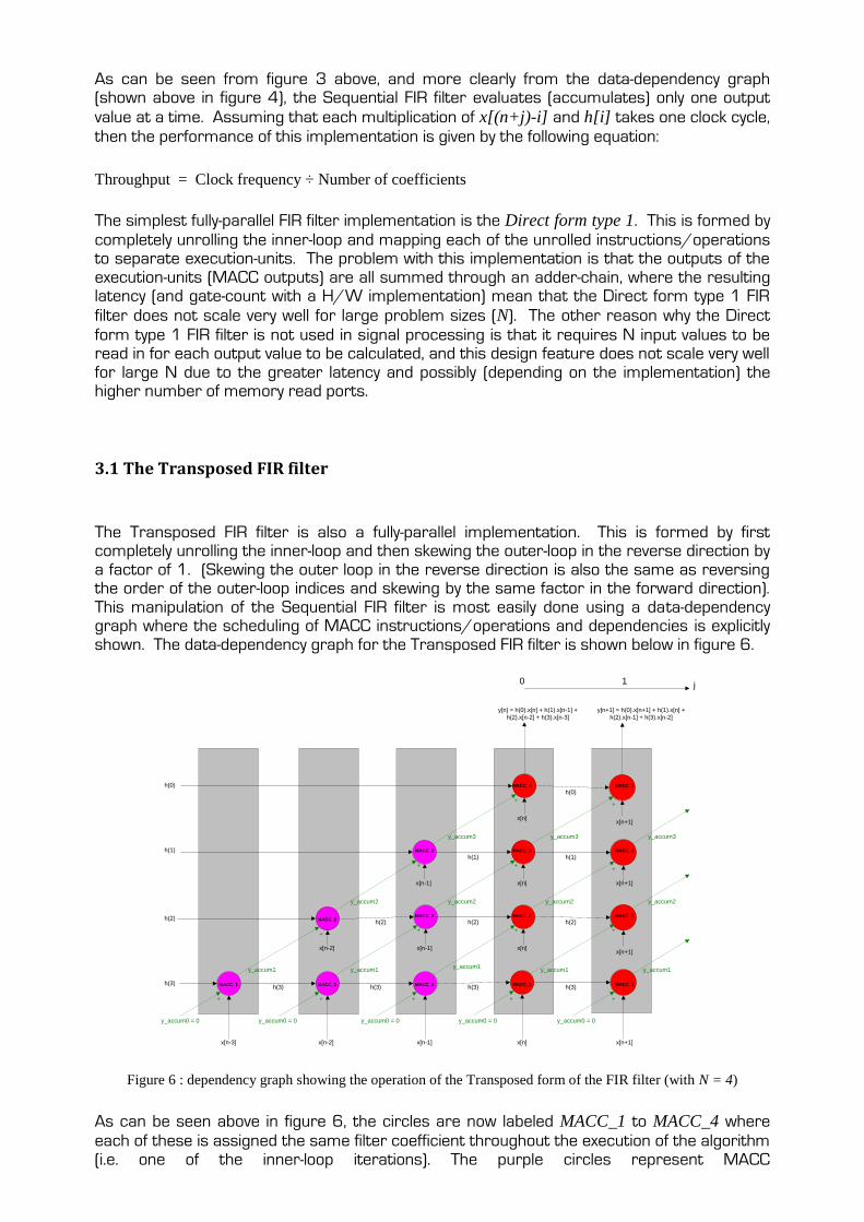
The Transposed FIR filter is also a fully-parallel implementation. This is formed by first completely unrolling the inner-loop and then skewing the outer-loop in the reverse direction by a factor of 1. (Skewing the outer loop in the reverse direction is also the same as reversing the order of the outer-loop indices and skewing by the same factor in the forward direction). This manipulation of the Sequential FIR filter is most easily done using a data-dependency graph where the scheduling of MACC instructions/operations and dependencies is explicitly shown. The data-dependency graph for the Transposed FIR filter is shown below in figure 6.
h(0)
h(1)h(1)
h(2)
x[n]
+ +
+
+
++
x[n-3] x[n-2]
x[n-2]
x[n-1]
x[n-1]
x[n-1]
x[n]
x[n]
x[n]
h(3)
h(2)
h(3)h(3)
h(2)
h(3)
y[n] = h(0).x[n] + h(1).x[n-1] +
h(2).x[n-2] + h(3).x[n-3]
+
+
+
x[n+1]
x[n+1]
x[n+1]
h(0)
h(1)
h(2)
h(3)
x[n+1]
y[n+1] = h(0).x[n+1] + h(1).x[n] +
h(2).x[n-1] + h(3).x[n-2]
y_accum0 = 0
j
MACC_1 MACC_1 MACC_1 MACC_1 MACC_1
MACC_2MACC_2 MACC_2 MACC_2
MACC_3 MACC_3 MACC_3
MACC_4 MACC_4
+++++
y_accum0 = 0 y_accum0 = 0 y_accum0 = 0 y_accum0 = 0
y_accum1 y_accum1y_accum1
y_accum1 y_accum1
y_accum2 y_accum2 y_accum2 y_accum2
y_accum3 y_accum3 y_accum3
0 1
Figure 6 : dependency graph showing the operation of the Transposed form of the FIR filter (with N = 4)
As can be seen above in figure 6, the circles are now labeled MACC_1 to MACC_4 where
each of these is assigned the same filter coefficient throughout the execution of the algorithm (i.e. one of the inner-loop iterations). The purple circles represent MACC
instructions/operations that occur during the spin-up process, which is the process of filling
the pipeline. The pipeline can either consist of N separate execution-units, or one execution-
unit which itself consists of N separate stages that have the same latency.
The skewing of the outer-loop results in temporal overlapping of successive output sample calculations. This temporal overlapping schedules apart the dependent MACC instructions/operations within a single iteration of the outer-loop, and this provides several advantages over the Direct form type 1 implementation.
Once the spin-up procedure is complete only one input data value is read per output value calculated. In the Transposed implementation this input value is then simultaneously
broadcasted to all of the N execution-units. These data-values are read in time-order meaning
that the input can be streamed in, and this lends itself very well to signal processing, where the objective is to process large amounts of data quickly.
The other advantage over the Direct form type 1 is that the MACC results summed to form each output value are done so using an adder chain, and as such the Transposed
implementation scales up very well for large and arbitrary values of N.
The disadvantage of the Transposed implementation is that latency of the spin-up and spin-
down (opposite of spin-down) procedures which are each N-1 cycles long. This latency is not
seen with the Direct form type 1 implementation, however the more output values that are
calculated the more this overhead is amortized. During the time the pipeline is full the
throughput is equal to the frequency with which successive MACC instructions/operations are executed, and this is equal to the throughput of the Direct form type 1 implementation. Another disadvantage with the Transposed implementation is that the number of filter taps is
limited by the fan-out capability of the register driving the common input of all the execution-
units with the input data value.
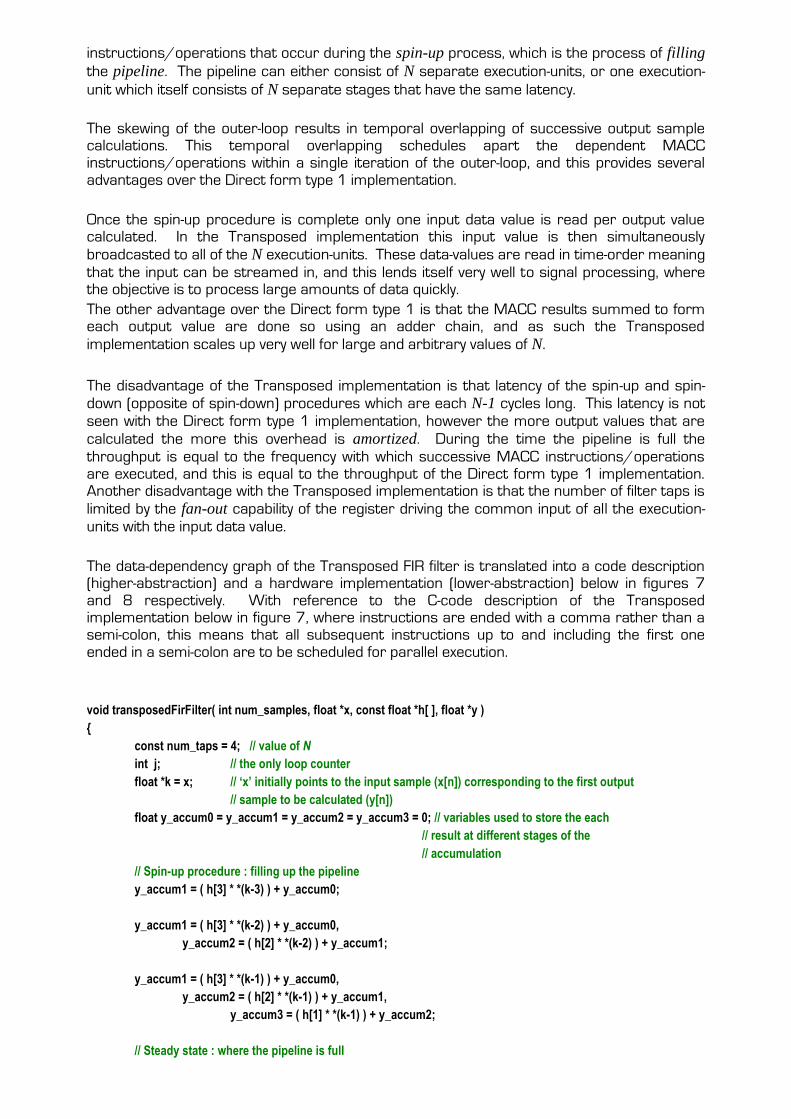
The data-dependency graph of the Transposed FIR filter is translated into a code description (higher-abstraction) and a hardware implementation (lower-abstraction) below in figures 7 and 8 respectively. With reference to the C-code description of the Transposed implementation below in figure 7, where instructions are ended with a comma rather than a semi-colon, this means that all subsequent instructions up to and including the first one ended in a semi-colon are to be scheduled for parallel execution.
void transposedFirFilter( int num_samples, float *x, const float *h[ ], float *y )
{
const num_taps = 4; // value of N
int j; // the only loop counter
float *k = x; // ‘x’ initially points to the input sample (x[n]) corresponding to the first output
// sample to be calculated (y[n])
float y_accum0 = y_accum1 = y_accum2 = y_accum3 = 0; // variables used to store the each
// result at different stages of the
// accumulation
// Spin-up procedure : filling up the pipeline
y_accum1 = ( h[3] * *(k-3) ) + y_accum0;
y_accum1 = ( h[3] * *(k-2) ) + y_accum0,
y_accum2 = ( h[2] * *(k-2) ) + y_accum1;
y_accum1 = ( h[3] * *(k-1) ) + y_accum0,
y_accum2 = ( h[2] * *(k-1) ) + y_accum1,
y_accum3 = ( h[1] * *(k-1) ) + y_accum2;
// Steady state : where the pipeline is full

for( j = 0; j < (num_samples – (num_taps-1)); j++ )
{
// y points to the variable address where y[n+j] is to be written and is incremented (post
// assignment) to point to the variable address where the next output sample y[(n+j)+1] // is to be written
*y++ = ( h[0] * *k ) + y_accum3,
y_accum3 = ( h[1] * *k ) + y_accum2,
y_accum2 = ( h[2] * *k ) + y_accum1,
y_accum1 = ( h[3] * *k ) + y_accum0;
k = x++; // ‘x’ initially points to x[n+j] and is incremented (post assignment) to point to // x[(n+j)+1]
}
// Spin-down procedure : emptying the pipeline
*y++ = ( h[0] * *k ) + y_accum3,
y_accum3 = ( h[1] * *k ) + y_accum2,
y_accum2 = ( h[2] * *k ) + y_accum1;
*y++ = ( h[0] * *(k+1) ) + y_accum3,
y_accum3 = ( h[1] * *(k+1) ) + y_accum2;
*y++ = ( h[0] * *(k+2) ) + y_accum3;
}
Figure 7 : A C-code description of the Transposed FIR filter which is a translation of the data-dependency graph of
figure 6 above
y_accum0 = 0
y_accum1 y_accum2 y_accum3 y_out
h(3) h(2) h(1) h(0)
y_in
MACC_1 MACC_2 MACC_3 MACC_4
Figure 8 : showing the H/W implementation of the Transposed form of the FIR filter (with N = 4) which is a
translation of the data-dependency graph of figure 6 above
With reference to figure 8 above, the coefficients are assigned to the execution-units in descending order going from the first input to the adder chain to its output. The significance of this is discussed below in section 3.2.

3.2 The Systolic FIR filter
The Systolic FIR filter is another fully-parallel implementation, and is formed from the Sequential FIR filter by completely unrolling the inner-loop and skewing the outer-loop in the forward direction by a factor of 1. This manipulation of the Sequential FIR filter is depicted in the data-dependency graph of the Systolic FIR filter shown below in figure 9.
h(0)
h(1)
h(3)
h(0) h(0) h(0)
h(1)h(1)
h(2)
h(2)
x[n] x[n+1] x[n+2] x[n+3]
x[n-1]
x[n-2]
x[n-3]
x[n+4]
h(0)
h(1)
h(2)
h(3)
x[n]
x[n-1]
x[n-2]
x[n+1] x[n+2]
x[n]
+ +
+ +
+ +
+
++
y[n] = h(0).x[n] + h(1).x[n-1] +
h(2).x[n-2] + h(3).x[n-3]
y[n+1] = h(0).x[n+1] + h(1).x[n] +
h(2).x[n-1] + h(3).x[n-2]
x[n+3]
x[n+1]
x[n-1]
x[n+4]
x[n+2]
x[n]
j0 1
MACC_1 MACC_1 MACC_1 MACC_1 MACC_1
MACC_2 MACC_2 MACC_2 MACC_2
MACC_3 MACC_3 MACC_3
MACC_4 MACC_4
+ + + + +
y_accum0 = 0 y_accum0 = 0 y_accum0 = 0 y_accum0 = 0 y_accum0 = 0
y_accum1 y_accum1 y_accum1 y_accum1y_accum1
y_accum2 y_accum2 y_accum2 y_accum2
y_accum3 y_accum3 y_accum3
Figure 9 : dependency graph showing the operation of the Systolic form of the FIR filter
(with N=4) As previously with the Transposed implementation the Systolic implementation goes through a spin-up procedure (where the pipeline is filled, represented above in figure 9 by the purple circles) and a spin-down procedure (where the pipeline is emptied) and again both of these
last for N-1 cycles.
As with the Transposed implementation, when the pipeline of the Systolic FIR filter is full there is one input data value read per output value calculated, and as with the Transposed implementation these input values are read in time order, and as previously mentioned these are the properties desired when the input is streamed into the filter. With reference to figure 9 above it can be seen that the filter coefficients are assigned to the execution-units in the opposite order that they were with the Transposed implementation (as the outer-loop in each
case is skewed in opposite directions). This means that there is a latency of N MACC cycles
between an input data value being read and the corresponding output value having finished
being calculated. However this latency for the Direct form type 1 as well as the Transposed implementation was only 1 MACC cycle, although the spin-up latency (time for first output value to emerge after starting the filter) and the spin-down latency (time after last output value emerges before filter is stopped) is the same for both the Transposed and Systolic implementations. As previously explained in section 3.1 the Transposed implementation is not suitable for very
high values of N because of the way the same input data value is broadcast to all of the
MACCs. This Systolic implementation has no such limitation and thus is more suitable than the Transposed implementation for implementing a FIR with a large number of taps. This however comes at the cost of an additional register per execution-unit, and these transfer input data values between adjacent execution-units with a latency of 1 MACC cycle. Therefore
in summary depending on the implementation platform, there is a breakpoint for the size of N

below which it is preferable to use the Transposed implementation and above which it is preferable to use the Systolic implementation.
void systolicFirFilter( int num_samples, float *x, const float *h[], float *y )
{
const num_taps // value of N
int j; // the only loop counter
float *k = x++; // ‘x’ initially points to the input sample (x[n]) corresponding to the first
// output sample to be calculated (y[n])
register y_accum0 = y_accum1 = y_accum2 = y_accum3 = 0; // variables used to store the each // result at different stages of the accumulation
// Spin-up procedure : filling up the pipeline
y_accum1 = ( h[0] * *k ) + y_accum0;
k = x++;
y_accum2 = ( h[1] * *(k-2) ) + y_accum1,
y_accum1 = ( h[0] * *k ) + y_accum0;
k = x++;
y_accum3 = ( h[2] * *(k-4) ) + y_accum2,
y_accum2 = ( h[1] * *(k-2) ) + y_accum1,
y_accum1 = ( h[0] * *k ) + y_accum0;
// Steady state : where the pipeline remains full
for( j = 0; j < (num_samples – (num_taps-1)); j++ )
{
// ‘x’ initially points to x[n+j] and is incremented (post assignment) to point to x[(n+j)+1]
k = x++;
// y points to the variable’s address where y[n+j] is to be written and is incremented
// (post assignment) to point to the variable address where the next output sample
// y[(n+j)+1] is to be written
*y++ = ( h[3] * *(k-6) ) + y_accum3,
y_accum3 = ( h[2] * *(k-4) ) + y_accum2,
y_accum2 = ( h[1] * *(k-2) ) + y_accum1,
y_accum1 = ( h[0] * *k ) + y_accum0;
}
// Spin-down procedure : emptying the pipeline
k = x++;
*y++ = ( h[3] * *(k-6) ) + y_accum3,
y_accum3 = ( h[2] * *(k-4) ) + y_accum2,
y_accum2 = ( h[1] * *(k-2) ) + y_accum1;
k = x++;
*y++ = ( h[3] * *(k-6) ) + y_accum3,
y_accum3 = ( h[2] * *(k-4) ) + y_accum2;
k = x;
*y++ = ( h[0] * *(k-6) ) + y_accum3;
}
Figure 10 : A C-code description of the Systolic form of the FIR filter (with N = 4) which is a translation of the
data-dependency graph of figure 9 above
y_accum0 = 0
y_accum1 y_accum2 y_accum3 y_out
h(0) h(1) h(2) h(3)
y_in
MACC_1 MACC_2 MACC_3 MACC_4
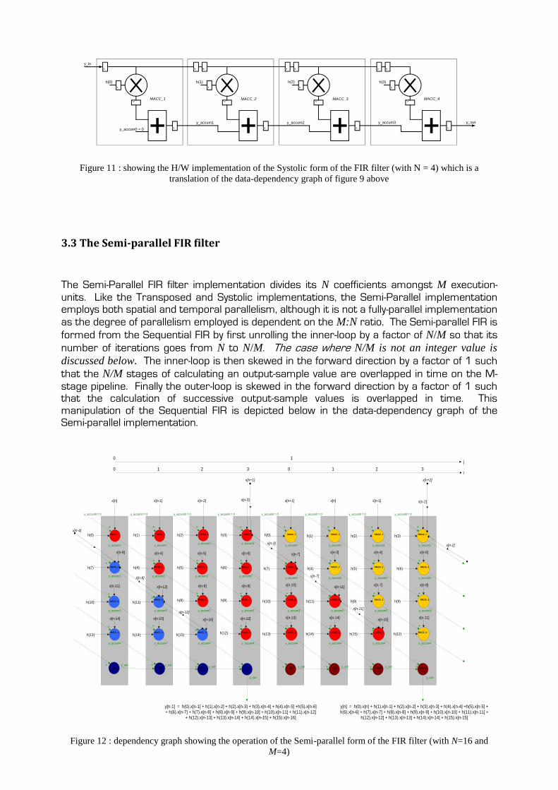
Figure 11 : showing the H/W implementation of the Systolic form of the FIR filter (with N = 4) which is a
translation of the data-dependency graph of figure 9 above
3.3 The Semi-parallel FIR filter
The Semi-Parallel FIR filter implementation divides its N coefficients amongst M execution-
units. Like the Transposed and Systolic implementations, the Semi-Parallel implementation employs both spatial and temporal parallelism, although it is not a fully-parallel implementation
as the degree of parallelism employed is dependent on the M:N ratio. The Semi-parallel FIR is
formed from the Sequential FIR by first unrolling the inner-loop by a factor of N/M so that its
number of iterations goes from N to N/M. The case where N/M is not an integer value is
discussed below. The inner-loop is then skewed in the forward direction by a factor of 1 such
that the N/M stages of calculating an output-sample value are overlapped in time on the M-
stage pipeline. Finally the outer-loop is skewed in the forward direction by a factor of 1 such that the calculation of successive output-sample values is overlapped in time. This manipulation of the Sequential FIR is depicted below in the data-dependency graph of the Semi-parallel implementation.
h(0) h(1) h(2) h(3)
h(6)h(5)
h(9)
x[n] x[n-1] x[n-2] x[n-3]
+ +
+ +
+ +
+
++
++
+
x[n-8]
x[n-11]
x[n-14] x[n-15]
x[n-12]
x[n-4]
x[n-16]
x[n-8]
x[n-5]
x[n-12]
x[n-9]
x[n-6]
h(12)
h(8)
h(15)h(14)
h(11)
h(4)
h(13)
h(10)
h(7)
x[n+1]
h(0)
+
+
+
x[n]
+
+
+
x[n-1]
+
+
+
x[n-2]
h(1) h(2) h(3)
h(7) h(4) h(5) h(6)
h(10) h(11) h(8) h(9)
h(13) h(14) h(15) h(12)
x[n-7]
x[n-10]
x[n-13]
x[n-11]
x[n-14]x[n-15]
x[n-3] x[n-4]
x[n-7]
x[n-5]
x[n-8]
x[n-11]
x[n-8]
x[n-12]
x[n-3]
x[n-7]
x[n-11]
x[n-2]
x[n-4]
+ + + + + +
y[n] = h(0).x[n] + h(1).x[n-1] + h(2).x[n-2] + h(3).x[n-3] + h(4).x[n-4] +h(5).x[n-5] +
h(6).x[n-6] + h(7).x[n-7] + h(8).x[n-8] + h(9).x[n-9] + h(10).x[n-10] + h(11).x[n-11] +
h(12).x[n-12] + h(13).x[n-13] + h(14).x[n-14] + h(15).x[n-15]
y[n-1] = h(0).x[n-1] + h(1).x[n-2] + h(2).x[n-3] + h(3).x[n-4] + h(4).x[n-5] +h(5).x[n-6]
+ h(6).x[n-7] + h(7).x[n-8] + h(8).x[n-9] + h(9).x[n-10] + h(10).x[n-11] + h(11).x[n-12]
+ h(12).x[n-13] + h(13).x[n-14] + h(14).x[n-15] + h(15).x[n-16]
x[n+1] x[n+2]
++
++
+
+
MACC_1 MACC_1 MACC_1 MACC_1 MACC_1 MACC_1 MACC_1 MACC_1
MACC_2 MACC_2 MACC_2 MACC_2 MACC_2 MACC_2 MACC_2 MACC_2
MACC_3MACC_3 MACC_3 MACC_3 MACC_3 MACC_3 MACC_3 MACC_3
MACC_4 MACC_4 MACC_4 MACC_4 MACC_4 MACC_4 MACC_4 MACC_4
ACC_1 ACC_1 ACC_1 ACC_1 ACC_1 ACC_1 ACC_1 ACC_1
++++++++
y_accum0 = 0 y_accum0 = 0 y_accum0 = 0 y_accum0 = 0 y_accum0 = 0 y_accum0 = 0 y_accum0 = 0 y_accum0 = 0
y_accum1 y_accum1y_accum1 y_accum1
y_accum1 y_accum1 y_accum1 y_accum1
y_accum2 y_accum2 y_accum2 y_accum2y_accum2 y_accum2 y_accum2 y_accum2
y_accum3 y_accum3 y_accum3 y_accum3 y_accum3 y_accum3 y_accum3 y_accum3
y_accum4 y_accum4 y_accum4 y_accum4 y_accum4 y_accum4 y_accum4 y_accum4
y_out y_outy_out y_out y_out y_out
y_out y_out
j0 1
0 1 2 3 0 1 2 3i
Figure 12 : dependency graph showing the operation of the Semi-parallel form of the FIR filter (with N=16 and
M=4)
The red circles represent MACC instructions/operations used to calculate the inner-
products of y[n], and the dark-red circles represent the output-accumulator being used to
accumulate the inner-products of y[n]. The blue and dark-blue circles represent the same for
y[n-1], whilst the yellow circles represent MACC instructions/operations used to calculate
the inner-products of y[n+1].
Each group of N/M coefficients is assigned to one of the execution-units and stored in order
within the associated coefficient-memory. The first group (coefficients 0 to (N/M – 1)) is
assigned to the top execution-unit (to which the input samples are applied), with ascending
coefficient groups being assigned to the execution-units from top to bottom (towards the
output-sample value accumulator). If N is not exactly integer-divisible by M, then the higher-
order coefficient-memories are padded with zeros.
As can be seen above in figure 12, the coefficient index for each execution-unit lies in the
range 0:((N/M) – 1) + offset where the offset increases by N/M between successive
execution-units going from the input to the output-accumulator. Figure 12 above also shows
how the MACC instructions/operations in the inner-loop are rescheduled so that after the M
instructions are mapped to the M execution-units the input-data stream can be kept in time-
order and divided into M chunks, where successive chunks in time are assigned to successive
execution-units going from the input to the output-accumulator. As seen above in figure 12, this means that between successive output-value calculations only one input-data value is
read in and each execution-unit shifts its oldest input-data value into the upstream adjacent
execution-unit in the pipeline. This yields the most efficient time overlapping of successive output-value calculations as there are no wasted MACC cycles. This temporal parallelism is in turn necessary to achieve the Semi-parallel implementation’s maximum throughput of one
output sample every N/M MACC cycles, because once an output sample has been retrieved
from the output-accumulator, the output-accumulator must be reset (to either zero or its
input value). For its input value to be the first sum of M inner-products of the next output
sample to be evaluated, then the evaluation of this sum needs to have finished in the previous MACC cycle, otherwise the output-accumulator will have to be reset to zero at the start of a
new calculation-cycle (i.e. outer-loop iteration). If the accumulator was set to zero between
calculation-cycles in this way, the time-overhead in setting up a new output-value calculation would be seen at the output, thus degrading performance.
A higher M:N ratio means the implementation is less folded and yields more parallelism both
spatially (as there are more execution-units employed) and temporally (as more inner-loop and outer-loop execution threads are scheduled for parallel execution). Thus the trade off is performance obtained versus the resources required, as can be seen by the equation for the performance of a Semi-parallel FIR filter implementation:
Throughput = ( Clock frequency ÷ N ) * M
The Semi-parallel implementation may be extrapolated either towards being a fully-parallel implementation like the Transposed and Systolic implementations by using more MACC units, or the other way towards being a Sequential FIR filter by using fewer MACC units. Figures 13 and 14 below show a C-code description and hardware implementation
respectively for the Semi-parallel FIR filter (again with N=16 and M=4).

void semi_parallelFirFilter( int num_taps, int num_samples, float *x, const float *h[ ], float *y )
{
int i, j;
int i0, i1, i2, i3;
float *k0, *k1, *k2, *k3;
register y_accum0 = 0, y_accum1 = 0, y_accum2 = 0, y_accum3 = 0, y_accum4 = 0, y_out = 0;
// Spin-up procedure
i0 = 0;
*k0 = x++;
y_accum1 = ( h[i0] * *k0 ) + y_accum0;
i1 = 4 + i0++;
k1 = (k0--) - 4;
y_accum2 = ( h[i1] * *k1 ) + y_accum1,
y_accum1 = ( h[i0] * *k0 ) + y_accum0;
i2 = i1 + 4, i1 = 4 + i0++;
*k2 = k1 – 4, *k1 = (k0--) – 4;
y_accum3 = ( h[i2] * *k2 ) + y_accum2,
y_accum2 = ( h[i1] * *k1 ) + y_accum1,
y_accum1 = ( h[i0] * *k0 ) + y_accum0;
i3 = i2 + 4, i2 = i1 + 4, i1 = 4 + i0++;
*k3 = k2 – 4, *k2 = k1 – 4, *k1 = (k0--) – 4;
y_accum4 = ( h[i3] * *k3 ) + y_accum3,
y_accum3 = ( h[i2] * *k2 ) + y_accum2,
y_accum2 = ( h[i1] * *k1 ) + y_accum1,
y_accum1 = ( h[i0] * *k0 ) + y_accum0;
// Steady state
i3 = i2 + 4, i2 = i1 + 4, i1 = 4 + i0, i0 = 0;
*k3 = k2 – 4, *k2 = k1 – 4, *k1 = (k0) – 4, *k0 = x++;
for(j = 0; j < (((num_taps / ‘4’) x num_samples) – ‘4’); j++ )
{
y_out = 0;
for(i = 0:3)
{
y_out += y_accum4,
y_accum4 = ( h[i3] * *k3 ) + y_accum3,
y_accum3 = ( h[i2] * *k2 ) + y_accum2,
y_accum2 = ( h[i1] * *k1 ) + y_accum1,
y_accum1 = ( h[i0] * *k0 ) + y_accum0;
i3 = i2 + 4, i2 = i1 + 4, i1 = i0 + 4, i0++;
*k3 = k2 – 4, *k2 = k1 – 4, *k1 = k0 – 4, *k0--;
}
*k0 = x++;
i0 = 0;
*y++ = y_out;
}
// Spin-down procedure
i3 = i2 + 4, i2 = i1 + 4, i1 = i0 + 4;
*k3 = k2 – 4, *k2 = k1 – 4, *k1 = k0 – 4;
y_out += y_accum4,
y_accum4 = ( h[i3] * *k3 ) + y_accum3,
y_accum3 = ( h[i2] * *k2 ) + y_accum2,
y_accum2 = ( h[i1] * *k1 ) + y_accum1;
i3 = i2 + 4, i2 = i1 + 4;
*k3 = k2 – 4, *k2 = k1 – 4;
y_out += y_accum4,
y_accum4 = ( h[i3] * *k3 ) + y_accum3,
y_accum3 = ( h[i2] * *k2 ) + y_accum2;
i3 = i2 + 4;
*k3 = k2 – 4;
y_out += y_accum4,
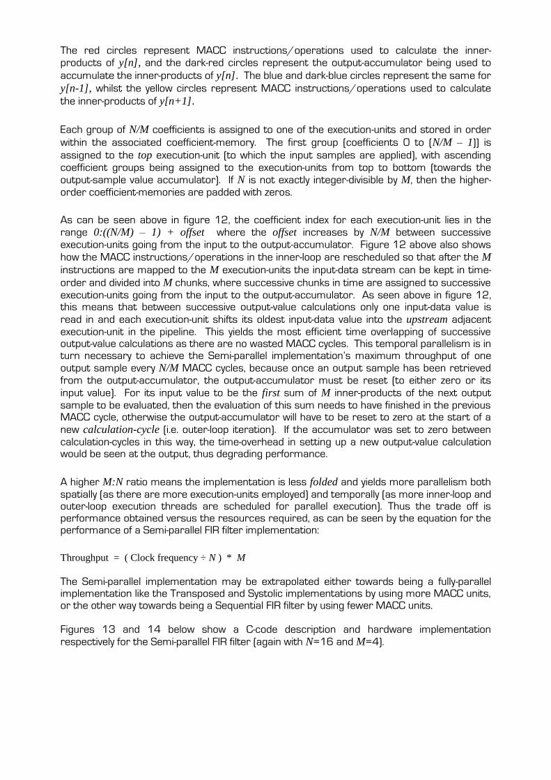
y_accum4 = ( h[i3] * *k3 ) + y_accum3;
y_out += y_accum4;
*y = y_out;
}
Figure 13 : a C-code description of the Semi-Parallel form of the FIR filter
(with N = 16, M = 4) which is a translation of the data-dependency graph of figure 12 above
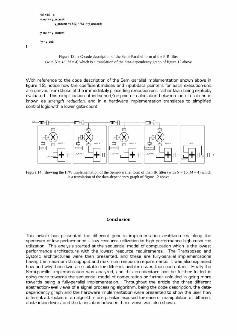
With reference to the code description of the Semi-parallel implementation shown above in figure 12, notice how the coefficient indices and input-data pointers for each execution-unit are derived from those of the immediately preceding execution-unit rather than being explicitly evaluated. This simplification of index and/or pointer calculation between loop iterations is
known as strength reduction, and in a hardware implementation translates to simplified
control logic with a lower gate-count.
y_accum0 = 0
y_accum1 y_accum2 y_accum3
y_in
MACC_1 MACC_2 MACC_3 MACC_4 ACC_1
h[0:N/M-1] h[N/M:2N/M-1] h[2N/M:3N/M-1] h[3N/M:4N/M-1]
y_out
y_accum4
Figure 14 : showing the H/W implementation of the Semi-Parallel form of the FIR filter (with N = 16, M = 4) which
is a translation of the data-dependency graph of figure 12 above
Conclusion
This article has presented the different generic implementation architectures along the spectrum of low performance – low resource utilization to high performance high resource utilization. This analysis started at the sequential model of computation which is the lowest performance architecture with the lowest resource requirements. The Transposed and Systolic architectures were then presented, and these are fully-parallel implementations having the maximum throughput and maximum resource requirements. It was also explained how and why these two are suitable for different problem sizes than each other. Finally the Semi-parallel implementation was analyzed, and this architecture can be further folded in going more towards the sequential model of computation or further unfolded in going more towards being a fully-parallel implementation. Throughout the article the three different abstraction-level views of a signal processing algorithm, being the code description, the data-dependency graph and the hardware implementation were presented to show the user how different attributes of an algorithm are greater exposed for ease of manipulation at different abstraction levels, and the translation between these views was also shown.