System of linear algebraic equation - sites.ualberta.cakumar/handouts/chap3.pdf · 3.1. MATRIX...

Mathematics, rightly viewed, possesses not onlytruth, but supreme beauty – a beauty cold and aus-tere, like that of sculpture.

— BERTRAND RUSSELL

Chapter 3

System of linear algebraicequation

Topics from linear algebra form the core of numerical analysis. Almostevery conceivable problem, be it curve fitting, optimization, simulationof flow sheets or simulation of distributed parameter systems requiringsolution of differential equations, require at some stage the solution of asystem (often a large system!) of algebraic equations. MATLAB (acronymfor MATrix LABoratory) was in fact conceived as a collection of tools toaid in the interactive learning and analysis of linear systems and wasderived from a well known core of linear algebra routines written inFORTRAN called LINPACK.

In this chapter we provide a quick review of concepts from linearalgebra. We make frequent reference to MATLAB implimentation of var-ious concepts throughout this chapter. The reader is encouraged to tryout these interactively during a MATLAB session. For a more completetreatment of topics in linear algebra see Hager (1985) and Barnett (1990).The text by Amundson (1966) is also an excellent source with specificexamples drawn from Chemical Engineering. For a more rigorous, ax-iomatic introduction within the frame work of linear opeartor theorysee Ramakrishna and Amundson (1985).

53

3.1. MATRIX NOTATION 54

3.1 Matrix notation

We have already used the matrix notation to write a system of linearalgebraic equations in a compact form in sections §1.3.1 and §1.3.2.While a matrix, as an object, is represented in bold face, its constituentelements are represented in index notation or as subscripted arrays inprogramming languages. For example the following are equivalent.

A = [aij], i = 1, · · · ,m; j = 1, · · · , nwhere A is an m×n matrix. aij represents an element of the matrix Ain row i and column j position. A vector can be thought of as an objectwith a single row or column. A row vector is represented by,

x = [x1 x2 · · ·xn]while a column vector can be represented by,

y =

y1

y2...ym

These elements can be real or complex.Having defined objects like vectors and matrices, we can extend the

notions of basic arithmetic opeartions between scalar numbers to higherdimensional objects like vectors and matrices. The reasons for doing soare many. It not only allows us to express a large system of equationsin a compact symbolic form, but a study of the properties of such ob-jects allows us to develop and codify very efficient ways of solving andanalysing large linear systems. Packages like MATLAB and Mathematicapresent to us a vast array of such codified algorithms. As an engineeryou should develop a conceptual understanding of the underlying prin-ciples and the skills to use such packages. But the most important taskis to indentify each element of a vector or a matrix, which is tied closelyto the physical description of the problem.

3.1.1 Review of basic operations

The arithmetic opeartions are defined both in symbolic form and usingindex notation. The later actually provides the algorithm for implement-ing the rules of operation using any programing language. The syntaxof these operations in MATLAB are shown with specific examples.∗

∗MATLAB illustrations have been tested with Ver 5.0.0.4064


The addition operation between two matrices is defined as,

addition: A = B + C ⇒ aij = bij + cij

This implies an element-by-element addition of the matrices B and C.Clearly all the matrices involved must have the same dimension. Notethat the addition operation is commutative as seen easily with its scalarcounter part. i.e.,

A + B = B + A

Matrix addition is also associative, i.e., independent of the order in whichit is carried out, e.g.,

A + B + C = (A + B) + C = A + (B + C)

The scalar multiplication of a matrix involves multiplying each elementof the matrix by the scalar, i.e.,

scalar multiplication: kA = B ⇒ k aij = bij

Subtraction operation can be handled by combining addition and sccalarmultiplication rules as follwos:

subtraction: C = A+ (−1)B = A − B ⇒ cij = aij − bij

The product between two matrices A (of dimension n ×m) and B (ofdimension m× r ) is defined as,

multiplication: C=AB ⇒ cij =m∑k=1

aikbkj ∀ i, j

and the resultant matrix has the dimension n × r . The operation in-dicated in the index notation is carried out for each value of the freeindices i = 1 · · · n and j = 1 · · · r . The product is defined only if thedimensions of B, C are compatible - i.e., number of columns in B shouldequal the number of rows in C. This implies that while the product BC may be defined, the product C B may not even be defined! Even whenthey are dimensionally compatible, in general

BC 6= BC

i.e., matrix multiplication is not commutative.


Example

Consider the matrices A, B defined below.

A =[

2 3 41 3 2

], B =

1 2

3 14 1

In MATLAB they will be defined as follows:

»A=[2 3 4;1 3 2] % Define (2x3) matrix A. Semicolon separates rows»B=[1 2; 3 1; 4 1]% Define (3x2) matrix B»C=A*B % calculate the productC= % Display the result[

27 1118 7

]

Other useful products can also be defined between vectors and matrices.A Hadamard (or Schur) product is defined as

C = A ◦ B ⇒ cij = aijbij ∀ i, j

Obviously, the dimension of A and B should be the same.

Example

The example below illustrates the Hadamard product, called the arrayproduct in MATLAB.

»C=A’.*B % Note the dimensions are made the same by transpose of AC= % Display the result 2 29 316 2

A Kronecker product is defined as

C = A ⊗ B ⇒ C =

a11B a12B · · · a1mBa21B a22B · · · a2mB

...an1B an2B · · · anmB


MATLAB functionthat generates theKronecker productbetween matricesisC=kron(A,B)

Multiplying a scalar number by unity leaves it unchanged. Extensionof this notion to matrices resutls in the definition of identity matrix, MATLAB function

for producing anidentity matrix ofsize N isI=eye(N)I =

1 0 · · · 00 1 · · · 0... 0 1 00 0 · · · 1

⇒ δij =

{1 i = j0 i 6= j

Multiplying any matrixA with an identity matrix I of appropriate dimen-sion leaves the original matrix unchanged, i.e.,

AI = AThis allows us to generalize the notion of division with scalar numbersto matrices. Division operation can be thought of as the inverse of the MATLAB function

for finding theinverse of a matrixA isB=inv(A)

multiplciation operation. For example, given a number, say 2, we candefine its inverse, x in such a way that the product of the two numbersproduce unity. i.e., 2 × x = 1 or x = 2−1. In a similar way, given amatrix A, can we define the inverse matrix B such that

AB = I or B = A−1

The task of developing an algorithm for finding the inverse of a matrixwill be addressed late in this chapter.

For a square matrix, powers of a matrix A can be defined as,

A2 = AA A3 = AAA = A2A = AA2

Note that ApAq = Ap+q for positve integers p and q. Having extended MATLAB operatorfor producing then-th power of amatrix A is,Aˆnwhile the syntaxfor producingelement-by-element poweris,A.ˆn.Make sure that youunderstand thedifference betweenthese twooperations!

the definition of powers, we can extend the definition of exponentialfrom scalars to square matrices as follows. For a scalar α it is,

MATLAB functionexp(A)evaluates theexponentialelement-by-elementwhileexpm(A)evaluates the truematrix exponential.

eα = 1 + α + α2

2+ · · · =

∞∑k=0

αk

k!

For a matrix A the exponential matrix can be defined as,

eA = I + A + A2

2+ · · · =

∞∑k=0

Ak

k!

One operation that does not have a direct counter part in the scalar worldis the transpose of a matrix. It is defined the result of exchanging therows and columns of a matrix, i.e.,

B = A′ ⇒ bij = aji

3.2. MATRICES WITH SPECIAL STRUCTURE 58

It is easy to verify that

(A + B)′ = A′ + B′

Something that is not so easy to verify, nevertheless true, is

(AB)′ = B′A′

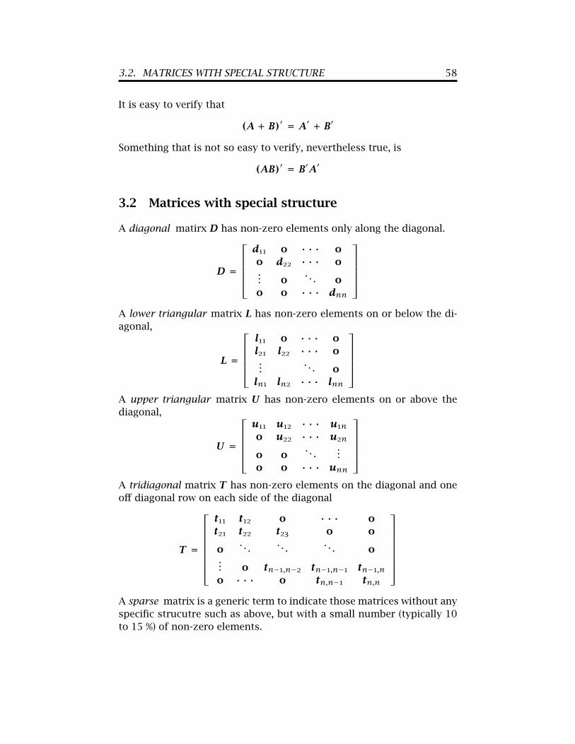
3.2 Matrices with special structure

A diagonal matirx D has non-zero elements only along the diagonal.

D =

d11 0 · · · 00 d22 · · · 0... 0

. . . 00 0 · · · dnn

A lower triangular matrix L has non-zero elements on or below the di-agonal,

L =

l11 0 · · · 0l21 l22 · · · 0...

. . . 0ln1 ln2 · · · lnn

A upper triangular matrix U has non-zero elements on or above thediagonal,

U =

u11 u12 · · · u1n0 u22 · · · u2n

0 0. . .

...0 0 · · · unn

A tridiagonal matrix T has non-zero elements on the diagonal and oneoff diagonal row on each side of the diagonal

T =

t11 t12 0 · · · 0t21 t22 t23 0 0

0. . . . . . . . . 0

... 0 tn−1,n−2 tn−1,n−1 tn−1,n0 · · · 0 tn,n−1 tn,n

A sparse matrix is a generic term to indicate those matrices without anyspecific strucutre such as above, but with a small number (typically 10to 15 %) of non-zero elements.

3.3. DETERMINANT 59

3.3 Determinant

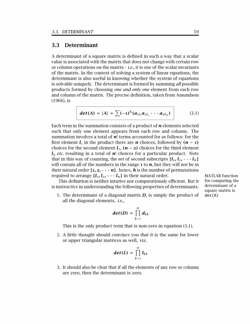
A determinant of a square matrix is defined in such a way that a scalarvalue is associated with the matrix that does not change with certain rowor column operations on the matrix - i.e., it is one of the scalar invariantsof the matrix. In the context of solving a system of linear equations, thedeterminant is also useful in knowing whether the system of equationsis solvable uniquely. The determinant is formed by summing all possibleproducts formed by choosing one and only one element from each rowand column of the matrix. The precise definition, taken from Amundson(1966), is

det(A) = |A| =∑(−1)h(a1l1a2l2 · · · anln) (3.1)

Each term in the summation consists of a product of n elements selectedsuch that only one element appears from each row and column. Thesummation involves a total of n! terms accounted for as follows: for thefirst element l1 in the product there are n choices, followed by (n − 1)choices for the second element l2, (n − 2) choices for the third elementl3 etc. resulting in a total of n! choices for a particular product. Notethat in this way of counting, the set of second subscripts {l1, l2, · · · ln}will contain all of the numbers in the range 1 to n, but they will not be intheir natural order {1, 2, · · · n}. hence, h is the number of permutationsrequired to arrange {l1, l2, · · · ln} in their natural order. MATLAB function

for computing thedeterminant of asquare matrix isdet(A)

This definition is neither intutive nor computationaly efficient. But itis instructive in understanding the following properties of determinants.

1. The determinant of a diagonal matrix D, is simply the product ofall the diagonal elements, i.e.,

det(D) =n∏k=1

dkk

This is the only product term that is non-zero in equation (3.1).

2. A little thought should convince you that it is the same for loweror upper triangular matrices as well, viz.

det(L) =n∏k=1

lkk

3. It should also be clear that if all the elements of any row or columnare zero, then the determinant is zero.

3.3. DETERMINANT 60

4. If every element of any row or column of a matrix is multipliedby a scalar, it is equivalent to multiplying the determinant of theoriginal matrix by the same scalar, i.e.,

∣∣∣∣∣∣∣∣∣∣

ka11 ka12 · · · ka1na21 a22 · · · a2n

.... . .

...an1 an2 · · · ann

∣∣∣∣∣∣∣∣∣∣=

∣∣∣∣∣∣∣∣∣∣

a11 a12 · · · ka1na21 a22 · · · ka2n

.... . .

...an1 an2 · · · kann

∣∣∣∣∣∣∣∣∣∣= kdet(A)

5. Replacing any row (or column) of a matrix with a linear combinationof that row (or column) and another row (or column) leaves thedeterminant unchanged.

6. A consequence of rules 3 and 5 is that if two rows (or columns) ofa matrix are indentical the determinant is zero.

7. If any two rows (or columns) are interchanged, it results in a signchange of the determinant.

3.3.1 Laplace expansion of the determinant

A definition of determinant that you might have seen in an earlier linearalgebra course is

det(A) = |A| ={ ∑n

k=1 aikAik for any i∑nk=1 akjAkj for any j (3.2)

where Aik, called the cofactor, is given by,

Aik = (−1)i+kMik

andMik, called the minor, is the determinant of (n−1)×(n−1) submatrixof A obtained by deleting ith row and kth column of A. Note that theexpansion in equation (3.2) can be carried out along any row i or columnj of the original matrix A.

Example

Consider the matrix derived in Chapter 1 for the recycle example, viz.equation (1.8). Let us calculate the determinant of the matrix using the

3.4. DIRECT METHODS 61

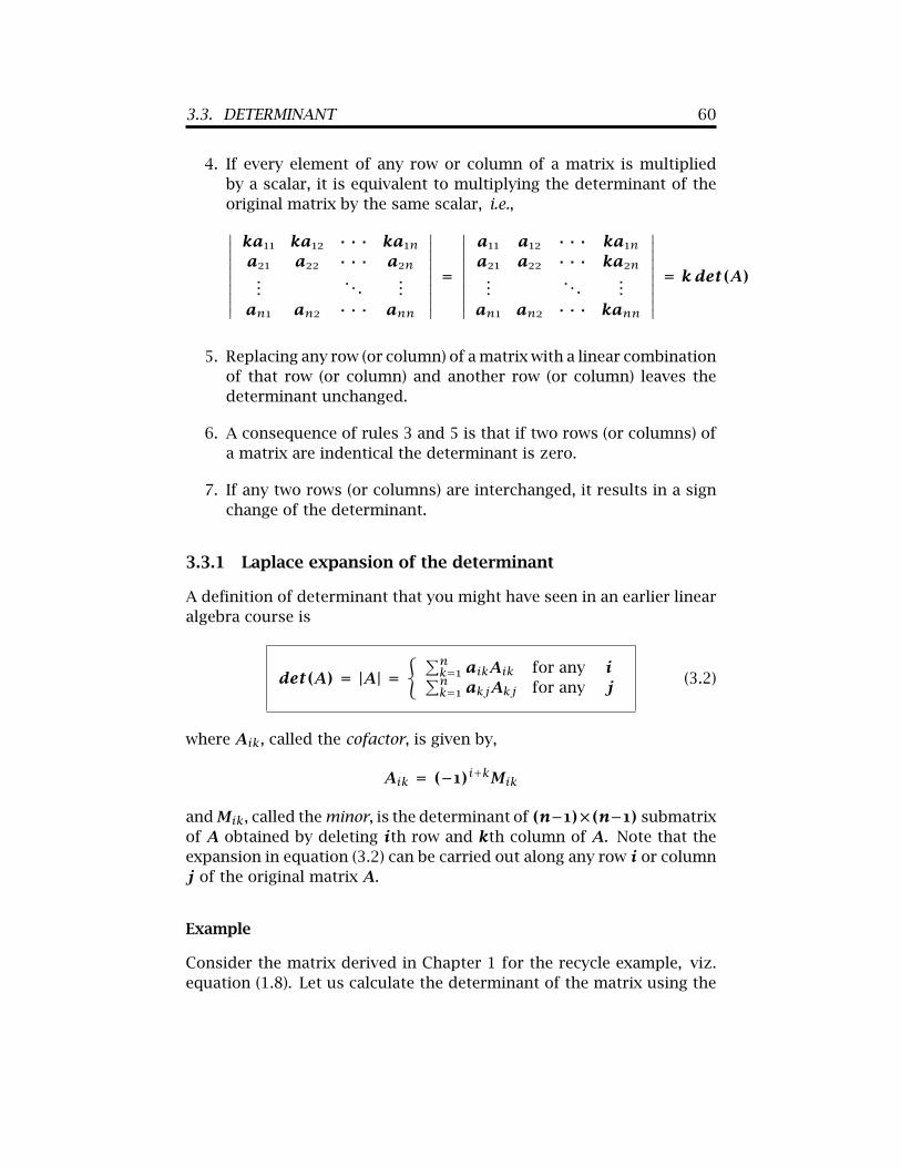
Laplace expansion algorithm around the first row.

det(A) =∣∣∣∣∣∣∣1 0 0.3060 1 0.702−2 1 0

∣∣∣∣∣∣∣

= 1

∣∣∣∣∣ 1 0.7021 0

∣∣∣∣∣ + (−1)1+2 × 0 ×∣∣∣∣∣ 0 0.702−2 0

∣∣∣∣∣ + (−1)1+3 × 0.306 ×∣∣∣∣∣∣0 1

−2 1

∣∣∣∣∣∣= 1 × (−0.702) + 0 + 0.306 × 2 = −0.09

A MATLAB implementation of this will be done as follows:

»A=[1 0 0.306; 0 1 0.702; -2 1 0] % Define matrix A»det(A) % calculate the determinant

3.4 Solving a system of linear equations

3.4.1 Cramers rule

Consider a 2 × 2 system of equations,[a11 a12a21 a22

] [x1x2

]=[b1b2

]

Direct elimination of the variable x2 results in

(a11a22 − a12a21) x1 = a22b1 − a12b2which can be written in an laternate form as,

det(A) x1 = det(A(1))where the matrix A(1) is obtained fromA after replacing the first columnwith the vector b. i.e.,

A(1) =∣∣∣∣∣ b1 a12b2 a22

∣∣∣∣∣This generalizees to n × n system as follows,

x1 = det(A(1))det(A)

, · · · xk = det(A(k))det(A)

, · · · xn = det(A(n))det(A)

.

where A(k) is an n × n matrix obtained from A by replacing the kthcolumn with the vector b. It should be clear from the above that, in orderto have a unique solution, the determinant of A should be non-zero. Ifthe determinant is zero, then such matrices are called singular.


Example

Continuing with the recycle problem (equation (1.8) of Chapter 1), solu-tion using Cramer’s rule can be implemented with MATLAB as follows:

A x = b ⇒ 1 0 0.3060 1 0.702−2 1 0

x1x2x3

=

101.48225.78

0

»A=[1 0 0.306; 0 1 0.702; -2 1 0]; % Define matrix A»b=[101.48 225.78 0]’ % Define right hand side vector b»A1=[b, A(:,[2 3])] % Define A(1)»A2=[A(:,1),b, A(:, 3)] % Define A(2)»A3=[A(:,[1 2]), b ] % Define A(3)»x(1) = det(A1)/det(A) % solve for coponent x(1)»x(2) = det(A2)/det(A) % solve for coponent x(2)»x(3) = det(A3)/det(A) % solve for coponent x(3)»norm(A*x’-b) % Check residual

3.4.2 Matrix inverse

We defined the inverse of a matrix A as that matrix B which, when mul-tiplied by A produces the identity matrix - i.e., AB = I; but we did notdevelop a scheme for findingB. We can do so now by combining Cramer’srule and Laplace expansion for a determinant as follows. Using Laplaceexpansion of the determinant of A(k) around column k,

detA(k) = b1A1k + b2A2k + · · · + bnAnk k = 1, 2, · · · , nwhereAik are the cofactors ofA. The components of the solution vector,x are,

x1 = (b1A11 + b2A21 + · · · + bnAn1)/det(A)xj = (b1A1j + b2A2j + · · · + bnAnj)/det(A)xn = (b1A1n + b2A2n + · · · + bnAnn)/det(A)

The right hand side of this system of equations can be written as a vectormatrix product as follows,

x1x2...xn

=

1det(A)

A11 A21 · · · An1A12 A22 · · · An2

.... . .

...A1n A2n · · · Ann

b1b2...bn


or

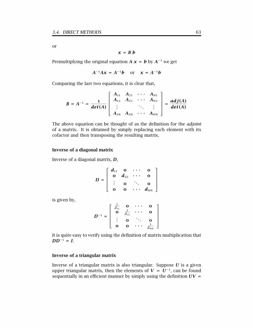
x = B bPremultiplying the original equation A x = b by A−1 we get

A−1Ax = A−1b or x = A−1b

Comparing the last two equations, it is clear that,

B = A−1 = 1det(A)

A11 A21 · · · An1A12 A22 · · · An2

.... . .

...A1n A2n · · · Ann

=

adj(A)det(A)

The above equation can be thought of as the definition for the adjointof a matrix. It is obtained by simply replacing each element with itscofactor and then transposing the resulting matrix.

Inverse of a diagonal matrix

Inverse of a diagonal matrix, D,

D =

d11 0 · · · 00 d22 · · · 0... 0

. . . 00 0 · · · dnn

is given by,

D−1 =

1d11 0 · · · 00 1

d22 · · · 0... 0

. . . 00 0 · · · 1

dnn

It is quite easy to verify using the definition of matrix multiplication thatDD−1 = I.

Inverse of a triangular matrix

Inverse of a triangular matrix is also triangular. Suppose U is a givenupper triangular matrix, then the elements of V = U−1, can be foundsequentially in an efficient manner by simply using the definition UV =


I. This equation, in expanded form, isu11 u12 · · · u1n0 u22 · · · u2n

0 0. . .

...0 0 · · · unn

v11 v12 · · · v1nv21 v22 · · · v2n

. . ....

vn1 vn2 · · · vnn

=

1 0 · · · 00 1 · · · 0

. . ....

0 0 · · · 1

We can develop the algorithm ( i.e., find out the rules) by simply carry-ing out the matrix multiplication on the left hand side and equating itelement-by-element to the right hand side. First let us convince ourselfthat V is also upper triangular, i.e.,

vij = 0 i > j (3.3)

Consider the element (n, 1) which is obtained by summing the productof each element of n-th row of U (consisting mostly of zeros!) with thecorresponding element of the 1-st column of V . The only non-zero termin this product is

unnvn1 = 0Since unn 6= 0 it is clear that vn1 = 0. Carrying out similar argumentsin a sequential manner (in the order {i = n · · · j − 1, j = 1 · · · n} -i.e., decreasing order of i and increasing order of j) it is easy to verifyequation (3.3) and thus establish that V is also upper triangular.

The non-zero elements of V can also be found in a sequential manneras follows. For each of the diagonal elements (i, i) summing the productof each element of i-th row of U with the corresponding element of thei-th column of V , the only non-zero term is,

vii = 1uii

i = 1, · · · , n (3.4)

Next, for each of the upper elements (i, j) summing the product ofeach element of i-th row of U with the corresponding element of thej-th column of V , we get,

uiivij +j∑

r=i+1uirvrj = 0

and hence we get,

vij = − 1uii

j∑r=i+1

uirvrj j = 2, · · · , n; j > i; i = j − 1, 1

(3.5)


Note that equation (3.5) should be applied in a specific order, as oth-erwise, it may involve unknown elements vrj on the right hand side.First, all of the diagonal elements of V ( viz. vii) must be calcualted fromequation (3.4) as they are needed on the right hand side of equation (3.5).Next the order indicated in equation (3.5), viz. increasing j from 2 to nand for each j decreasing i from (j − 1) to 1, sould be obeyed to avoidhaving unknowns values appearing on the right hand side of (3.5).

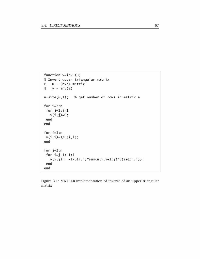
A MATLAB implementation of this algorithm is shown in figure 3.1to illustrate precisely the order of the calculations. Note that the built-in, general purpose MATLAB inverse function ( viz. inv(U) ) does nottake into account the special structure of a triangular matrix and henceis computationally more expensive than the invu funcion of figure 3.1.This is illustrated with the following example.

Example

Consider the upper triangular matrix,

U =

1 2 3 40 2 3 10 0 1 20 0 0 4

Let us find its inverse using both the built-in MATLAB function inv(U)and the function invu(U) of figure 3.1 that is applicable sepcifically foran upper triangular matrix. You can also compare the floating pointopeartion count for each of the algorithm. Work through the followingexample using MATLAB. Make sure that the function invu of figure 3.1is in the search path of MATLAB.

» U=[1 2 3 4; 0 2 3 1;0 0 1 2; 0 0 0 4]

U =

1 2 3 40 2 3 10 0 1 20 0 0 4

» flops(0) %initialize the flop count» V=inv(U)


V =

1.0000 -1.0000 0 -0.75000 0.5000 -1.5000 0.62500 0 1.0000 -0.50000 0 0 0.2500

» flops %print flop count

ans =

208» flops(0);ch3_invu(U),flops %initialize flop count, then invert

ans =

1.0000 -1.0000 0 -0.75000 0.5000 -1.5000 0.62500 0 1.0000 -0.50000 0 0 0.2500

ans =

57

3.4.3 Gaussian elimination

Gaussian elimination is one of the most efficient algorithms for solvinga large system of linear algebraic equations. It is based on a systematicgeneralization of a rather intuitive elimination process that we routinelyapply to a small, say, (2 × 2) systems. e.g.,

10x1 + 2x2 = 4

x1 + 4x2 = 3From the first equation we have x1 = (4 − 2x2)/10 which is used toeliminate the variable x1 from the second equation, viz. (4− 2x2)/10+4x2 = 3 which is solved to get x2 = 0.6842. In the second phase, the


function v=invu(u)% Invert upper triangular matrix% u - (nxn) matrix% v - inv(a)

n=size(u,1); % get number of rows in matrix a

for i=2:nfor j=1:i-1v(i,j)=0;

endend

for i=1:nv(i,i)=1/u(i,i);end

for j=2:nfor i=j-1:-1:1v(i,j) = -1/u(i,i)*sum(u(i,i+1:j)*v(i+1:j,j));

endend

Figure 3.1: MATLAB implementation of inverse of an upper triangularmatrix


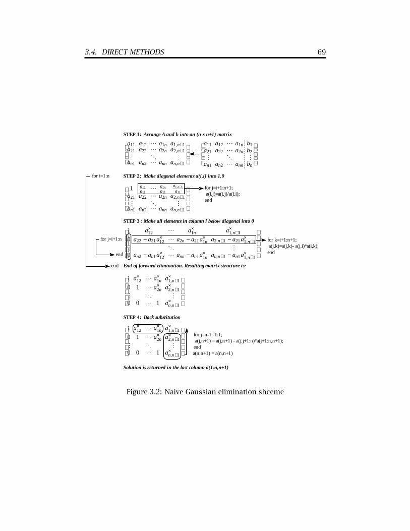
value of x2 is back substituted into the first equation and we get x1 =0.2632. We could have reversed the order and eliminated x1 from thefirst equation after rearranging the second equation as x1 = (3 − 4x2).Thus there are two phases to the algorithm: (a) forward elimination ofone variable at a time until the last equation contains only one unknown;(b) back substitution of variables. Also, note that we have used two rulesduring the elimination process: (i) two equations (or two rows) can beinterchanged as it is merely a matter of book keeping and it does not inany way alter the problem formulation, (ii) we can replace any equationwith a linear combination of itself with another equation. A conceptualdescription of a naive Gaussian elimination algorithm is shown in figure3.2. All of the arithmetic operations needed to eliminate one variable ata time are identified in the illustration. Study that carefully.

We call it a naive scheme as we have assumed that none of the diag-onal elements are zero, although this is not a requirement for existenceof a solution. The reason for avoiding zeros on the diagoanls is to avoiddivision by zeros in step 2 of the illustration 3.2. If there are zeros onthe diagonal, we can interchange two equations in such a way the di-agonals do not contain zeros. This process is called pivoting. Even ifwe organize the equations in such a way that there are no zeros on thediagonal, we may end up with a zero on the diagonal during the elimina-tion process (likely to occur in step 3 of illustration 3.2). If that situationarises, we can continue to exchange that particular row with another oneto avoid division by zero. If the matrix is singular we wil eventually endup with an unavoidable zero on the diagonal. This situation will arise ifthe original set of equations is not linearly independent; in other wordsthe rank of the matrix A is less than n. Due to the finite precision ofcomputers, the floating point operation in step 3 of illustration 3.2 willnot result usually in an exact zero, but rather a very small number. Lossof precision due to round off errors is a common problem with directmethods involving large system of equations since any error introducedat one step corrupts all subsequent calcualtions.

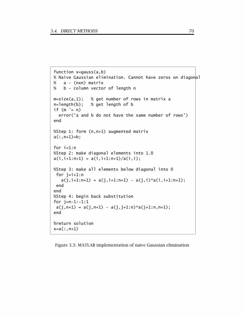
A MATLAB implementation of the algorithm is given in figure 3.3through the function gauss.m. Note that it is

merely forillustrating theconcepts involvedin the eliminationprocess; MATLABbackslash, \operator providesa much moreelegant solution tosolve Ax = b inthe form x = A\b.

Example

Let us continue with the recycle problem (equation (1.8) of Chapter 1).First we obtain solution using the built-in MATLAB linear equation solver( viz. x = A\b and record the floating point operations (flops). Thenwe solve with the Gaussian elimination function gauss and compare theflops. Note that in order to use the naive Gaussian elimination function,


ċ

ċ

� ? ? �

ċ

100

10

1

a

aa

aaa

+×

+××

+×××

1,

1,22

1,1121

nn

nn

nn

ċ

ċ

� ? ? �

ċ

−−−

−−−

0

0

1

aaaaaaaaa

aaaaaaaaa

aaa

+×

+××

+×

+××

+×××

1,111,112112

1,1121,21122211222

1,1121

nnnnnnnnnn

nnnn

nn

for j=i+1:n+1; a(i,j)=a(i,j)/a(i,i);end

for k=i+1:n+1; a(j,k)=a(j,k)- a(j,i)*a(i,k);end

STEP 2: Make diagonal elements a(i,i) into 1.0

STEP 1: Arrange A and b into an (n x n+1) matrix

STEP 3 : Make all elements in column i below diagonal into 0

for i=1:n

for j=i+1:n

end

End of forward elimination. Resulting matrix structure is:end

ċ

ċ

� ? ? �

ċ

baaa

baaabaaa

21

222212

112111

nnnnn

n

nċ

ċ

� ? ? �ċ

aaaa

aaaaaaaa

+

++

1,21

1,2222121,112111

nnnnnn

nnnn

ċ

ċ

� ? ? �

ċ

100

10

1

a

aa

aaa

+×

+××

+×××

1,

1,22

1,1121

nn

nn

nn

STEP 4: Back substitution

ċ

ċ

� ? ? �ċ

1

nnnnnn

nna

aaa

aa +

11

1,1

11

1

11

21 nn

aaaa

aaaa

+

+

1,21

1,222212

a(n,n+1) = a(n,n+1)

for j=n-1:-1:1; a(j,n+1) = a(j,n+1) - a(j,j+1:n)*a(j+1:n,n+1);end

Solution is returned in the last column a(1:n,n+1)

Figure 3.2: Naive Gaussian elimination shceme


function x=gauss(a,b)% Naive Gaussian elimination. Cannot have zeros on diagonal% a - (nxn) matrix% b - column vector of length n

m=size(a,1); % get number of rows in matrix an=length(b); % get length of bif (m ˜= n)error(’a and b do not have the same number of rows’)

end

%Step 1: form (n,n+1) augmented matrixa(:,n+1)=b;

for i=1:n%Step 2: make diagonal elements into 1.0a(i,i+1:n+1) = a(i,i+1:n+1)/a(i,i);

%Step 3: make all elements below diagonal into 0for j=i+1:na(j,i+1:n+1) = a(j,i+1:n+1) - a(j,i)*a(i,i+1:n+1);

endend%Step 4: begin back substitutionfor j=n-1:-1:1a(j,n+1) = a(j,n+1) - a(j,j+1:n)*a(j+1:n,n+1);end

%return solutionx=a(:,n+1)

Figure 3.3: MATLAB implementation of naive Gaussian elimination


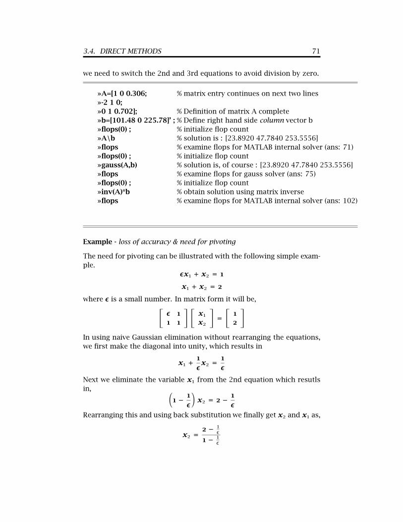
we need to switch the 2nd and 3rd equations to avoid division by zero.

»A=[1 0 0.306; % matrix entry continues on next two lines»-2 1 0;»0 1 0.702]; % Definition of matrix A complete»b=[101.48 0 225.78]’ ; % Define right hand side column vector b»flops(0) ; % initialize flop count»A\b % solution is : [23.8920 47.7840 253.5556]»flops % examine flops for MATLAB internal solver (ans: 71)»flops(0) ; % initialize flop count»gauss(A,b) % solution is, of course : [23.8920 47.7840 253.5556]»flops % examine flops for gauss solver (ans: 75)»flops(0) ; % initialize flop count»inv(A)*b % obtain solution using matrix inverse»flops % examine flops for MATLAB internal solver (ans: 102)

Example - loss of accuracy & need for pivoting

The need for pivoting can be illustrated with the following simple exam-ple.

εx1 + x2 = 1x1 + x2 = 2

where ε is a small number. In matrix form it will be,[ε 11 1

] [x1x2

]=[12

]

In using naive Gaussian elimination without rearranging the equations,we first make the diagonal into unity, which results in

x1 + 1εx2 = 1

ε

Next we eliminate the variable x1 from the 2nd equation which resutlsin, (

1 − 1ε

)x2 = 2 − 1

εRearranging this and using back substitution we finally get x2 and x1 as,

x2 =2 − 1

ε1 − 1

ε


Naive elimination Built-inε without pivoting MATLAB

gauss(A,b) A\b1 × 10−15 [1 1] [1, 1]1 × 10−16 [2 1] [1, 1]1 × 10−17 [0 1] [1, 1]

Table 3.1: Loss of precision and need for pivoting

x1 = 1ε− x2ε

The problem in computing x1 as ε → 0 should be clear now. As εcrosses the threshold of finite precision of the computation (hardwareor software), taking the difference of two large numbers of comparablemagnitude, can result in significant loss of precision. Let us solve theproblem once again after rearranging the equations as,

x1 + x2 = 2εx1 + x2 = 1

and apply Gaussian elimination once again. Since the diagonal elementin the first equation is already unity, we can eliminate x1 from the 2ndequation to obtain,

(1 − ε)x2 = 1 − 2ε or x2 = 1 − 2ε1 − ε

Back substitution yields,x1 = 2 − x2

Both these computations are well behaved as ε → 0.We can actually demonstrate this using the MATLAB function gauss

shown in figure 3.3 and compare it with the MATLAB built-in functionA\b which does use pivoting to rearrange the equations and minimizethe loss of precision. The results are compared in table 3.1 for ε inthe range of 10−15 to 10−17. Since MATLAB uses double precision, thisrange of ε is the threshold for loss of precision. Observe that the naiveGaussian elimination produces incorrect results for ε < 10−16.

3.4.4 Thomas algorithm

Many problems such as the stagewise separation problem we saw in sec-tion §1.3.1 or the solution of differential equations that we will see in


??

?

? ? ?

bdbcd

bcdbcd

∗∗−

∗−−

∗

∗∗

111

222

111

0000

000000

nn

nnn

d(j) = d(j) - {a(j-1)/d(j-1)}*c(j-1) b(j) = b(j) - {a(j-1)/d(j-1)}*b(j-1)

STEP 1: Eliminate lower diagonal elements

Given

STEP 2: Back substitution

for i=n-1:-1:1 b(i) = {b(i) - c(i)*b(i+1)}/d(i);end

b(n) = b(n)/d(n)

Solution is stored in b

??

?

? ? ?

bdabcda

bcdabcd

−−−−−

1

1112

2221

111

0000

000

nnn

nnnn

for j=2:n

end

??

?

? ? ?

bdbcd

bcdbcd

∗∗−

∗−−

∗

∗∗

111

222

111

0000

000000

nn

nnn

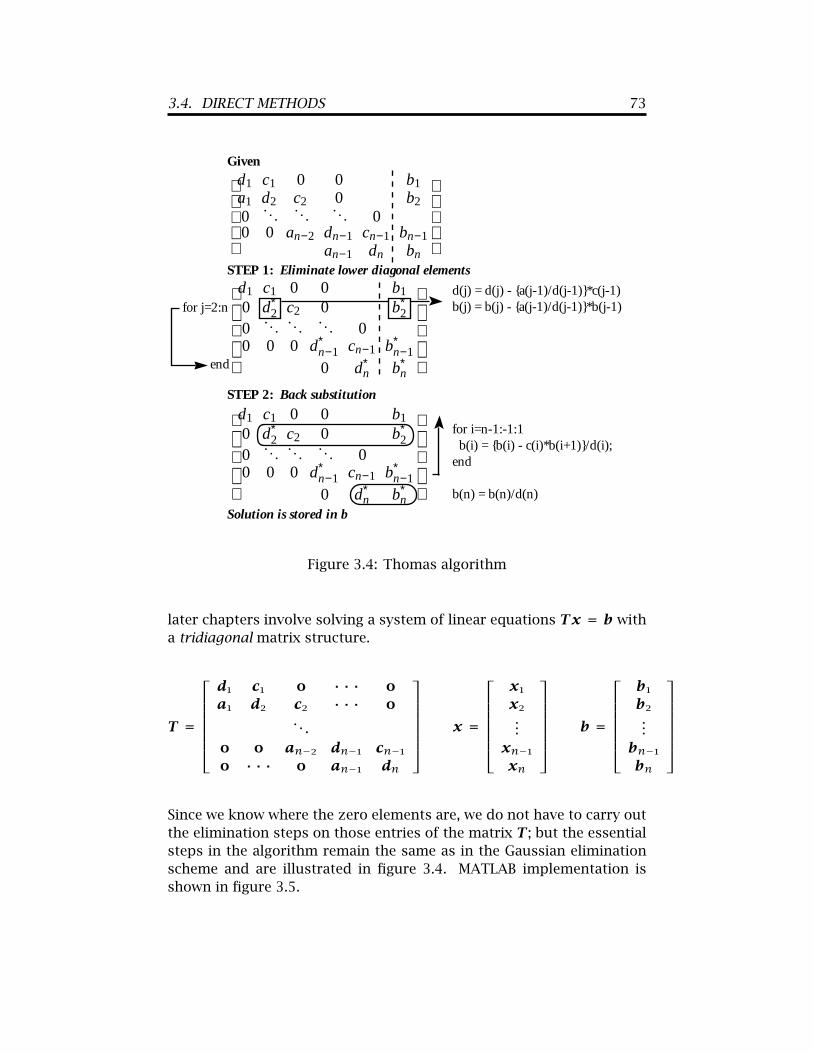
Figure 3.4: Thomas algorithm

later chapters involve solving a system of linear equations Tx = b witha tridiagonal matrix structure.

T =

d1 c1 0 · · · 0a1 d2 c2 · · · 0

. . .0 0 an−2 dn−1 cn−10 · · · 0 an−1 dn

x =

x1x2...

xn−1xn

b =

b1b2...

bn−1bn

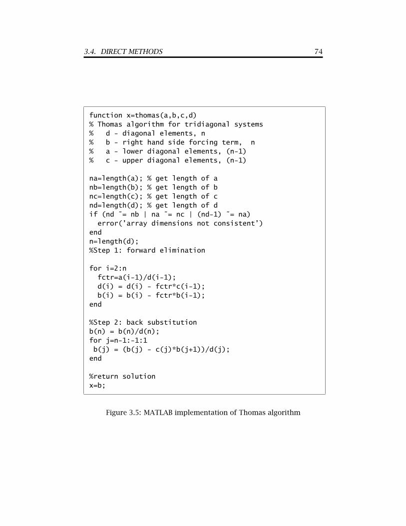
Since we know where the zero elements are, we do not have to carry outthe elimination steps on those entries of the matrix T ; but the essentialsteps in the algorithm remain the same as in the Gaussian eliminationscheme and are illustrated in figure 3.4. MATLAB implementation isshown in figure 3.5.


function x=thomas(a,b,c,d)% Thomas algorithm for tridiagonal systems% d - diagonal elements, n% b - right hand side forcing term, n% a - lower diagonal elements, (n-1)% c - upper diagonal elements, (n-1)

na=length(a); % get length of anb=length(b); % get length of bnc=length(c); % get length of cnd=length(d); % get length of dif (nd ˜= nb | na ˜= nc | (nd-1) ˜= na)error(’array dimensions not consistent’)

endn=length(d);%Step 1: forward elimination

for i=2:nfctr=a(i-1)/d(i-1);d(i) = d(i) - fctr*c(i-1);b(i) = b(i) - fctr*b(i-1);

end

%Step 2: back substitutionb(n) = b(n)/d(n);for j=n-1:-1:1b(j) = (b(j) - c(j)*b(j+1))/d(j);end

%return solutionx=b;

Figure 3.5: MATLAB implementation of Thomas algorithm


3.4.5 Gaussian elimination - Symbolic representaion

Given a square matrix A of dimension n × n it is possible to write it isas the product of two matrices B and C, i.e., A = BC. This process iscalled factorization and is in fact not at all unique - i.e., there are inifnitelymany possiblilities for B and C. This is clear with a simple counting ofthe unknowns - viz. there are 2×n2 unknown elements in B and C whileonly n2 equations can be obtained by equating each element of A withthe corresponding element from the product BC.

The extra degrees of freedom can be used to specify any specificstructure for B and C. For example we can require B = L be a lowertriangular matrix and C = U be an upper triangular matrix.This processis called LU factorization or decomposition. Since each triangular matrixhas n × (n + 1)/2 unknowns, we still have a total of n2 + n unknowns.The extra n degrees of freedom is often used in one of three ways:

• Doolitle method assigns the diagonal elements of L to be unity.

• Crout method assigns the diagonal elements of U to be unity.

• Cholesky method assigns the diagonal elements of L to be equal tothat ofU - i.e., lii = uii.

While a simple degree of freedom analysis, indicates that it is possible tofactorize a matrix into a product of lower and upper trinagular matrices,it does not tell us how to find out the unknown elements.

Revisiting the Gaussian elimination method from a different perspec-tive, will show the connection between LU factorization and Gaussianelimination. Note that the algorithm outlined in section §3.4.3 is themost computationally efficient scheme for implimenting Guassian elimi-nation. The method to be outlined below is not computationally efficient,but it is a useful conceptual aid in showing the connection between Guas-sian elimination and LU factorization. Steps 2 and 3 of figure 3.2 thatinvolve making the diagonal into unity and all the elements below the di-agonal into zero is equivalent to pre-multuplying A by L1 - i.e., L1A = U1or,

1a11 0 · · · 0−a21a11 1 · · · 0

... 0. . . 0

−an1a11 0 0 1

a11 a12 · · · a1na21 a22 · · · a2n

. . ....

an1 an2 · · · ann

=

1 a(1)12 · · · a(1)1n0 a(1)22 · · · a(1)2n

. . ....

0 a(1)n2 · · · a(1)nn


Repeating this process for the 2nd row, we pre-multiply U1 by L2 - i.e.,L2U1 = U2 or, in expanded form,

1 0 0 · · · 00 1

a(1)220 · · · 0

0 −a(1)32

a(1)221 · · · 0

...... 0

. . . 0

0 −a(1)n2a(1)22

0 0 1

1 a(1)12 · · · a(1)1n0 a(1)22 · · · a(1)2n

. . ....

0 a(1)n2 · · · a(1)nn

=

1 a(1)12 a(1)13 · · · a(1)1n0 1 a(2)23 · · · a(2)2n

0 0 a(2)33 · · · ...

0 0... · · · ...

0 0 a(2)n3 · · · a(2)nn

Continuing this process, we obtain in succession,

L1A = U1

L2U1 = U2L3U2 = U3L4U3 = U4

Ln−1Un−2 = Un−1Note that each Lj is a lower triangular matrix with non-zero elements onthe j-th column and unity on other diagonal elements. Eliminating allof the intermediate Uj we obtain,

(Ln−1Ln−2 · · · L1)A = Un−1

Since the product of all lower triangular matrices is yet another lowertriangular matrix, we can write the above equation as,

LA = U

Also, the inverse of a lower triangular matrix is also lower triangular- i.e., L̂ = L−1. Hence a given square matrix A can be factored into aproduct of a lower and upper triangular matrix as,

A = L−1U = L̂U

Although the development in this section provides us with an algorithmfor constructing both L̂ and U , it is quite inefficient. A more direct andefficient algorithm is developed next in section §3.4.6.


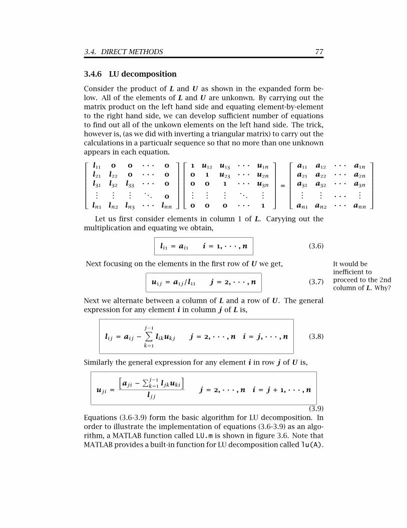
3.4.6 LU decomposition

Consider the product of L and U as shown in the expanded form be-low. All of the elements of L and U are unkonwn. By carrying out thematrix product on the left hand side and equating element-by-elementto the right hand side, we can develop sufficient number of equationsto find out all of the unkown elements on the left hand side. The trick,however is, (as we did with inverting a triangular matrix) to carry out thecalculations in a particualr sequence so that no more than one unknownappears in each equation.

l11 0 0 · · · 0l21 l22 0 · · · 0l31 l32 l33 · · · 0...

......

. . . 0ln1 ln2 ln3 · · · lnn

1 u12 u13 · · · u1n0 1 u23 · · · u2n0 0 1 · · · u3n...

......

. . ....

0 0 0 · · · 1

=

a11 a12 · · · a1na21 a22 · · · a2na31 a32 · · · a3n

...... · · · ...

an1 an2 · · · ann

Let us first consider elements in column 1 of L. Caryying out themultiplication and equating we obtain,

li1 = ai1 i = 1, · · · , n (3.6)

Next focusing on the elements in the first row of U we get, It would beinefficient toproceed to the 2ndcolumn of L. Why?

u1j = a1j/l11 j = 2, · · · , n (3.7)

Next we alternate between a column of L and a row of U . The generalexpression for any element i in column j of L is,

lij = aij −j−1∑k=1

likukj j = 2, · · · , n i = j, · · · , n (3.8)

Similarly the general expression for any element i in row j of U is,

uji =[aji −

∑j−1k=1 ljkuki

]ljj

j = 2, · · · , n i = j + 1, · · · , n

(3.9)Equations (3.6-3.9) form the basic algorithm for LU decomposition. Inorder to illustrate the implementation of equations (3.6-3.9) as an algo-rithm, a MATLAB function called LU.m is shown in figure 3.6. Note thatMATLAB provides a built-in function for LU decomposition called lu(A).


function [L,U]=LU(a)% Naive LU decomposition% a - (nxn) matrix% L,U - are (nxn) factored matrices% Usage [L,U]=LU(A)

n=size(a,1); % get number of rows in matrix a

%Step 1: first column of LL(:,1)=a(:,1);

%Step 2: first row of UU(1,:)=a(1,:)/L(1,1);

%Step 3: Alternate between column of L and row of Ufor j=2:nfor i = j:nL(i,j) = a(i,j) - sum(L(i,1:j-1)’.*U(1:j-1,j));

endU(j,j) = 1;for i=j+1:nU(j,i)=(a(j,i) - sum(L(j,1:j-1)’.*U(1:j-1,i) ) )/L(j,j);

endend

Figure 3.6: MATLAB implementation of LU decomposition algorithm


Recognizing that A can be factored into the product LU , one can im-plement an efficient scheme for solving a system of linear algebraic equa-tions Ax = b repeatedly, particularly when the matrix A remains un-changed, but different solutions are required for different forcing termson the right hand side, b. The equation

Ax = bcan be written as

LUx = b ⇒ Ux = L−1b = b′and hence

x = U−1b′The operations required for forward elimination and back substitutionare stored in the LU factored matrix and as we saw earlier it is rela-tively efficient to invert triangular matrices. Hence two additional vector-matrix products provide a solution for each new value of b.

Example

Work through the following exercise in MATLAB to get a feel for thebuilt-in MATLAB implementation of LU factorization with that given infigure 3.6. Before you work through the exercise make sure that the fileLU.m that contains the function illustrated in figure 3.6 is in the MATLABpath. Also, be aware of the upper case function LU of figure 3.6 and thelower case lu which is the built-in function.

»A=[1 0 0.306; 0 1 0.702; -2 1 0]; % Define matrix A»b=[101.48 225.78 0]’ % Define right hand vector b»flops(0) % initialize flop count»x=A\b % solve using built-in solver»flops % flops = 74»flops(0) % re-initialize flop count»[l,u]=LU(A) %Use algorithm in figure 3.6»flops % flops = 24»x=inv(u)*(inv(l)*b) % Solve linear system»flops % Cumulative flops = 213»flops(0) % re-initialize flop count»[L,U]=lu(A) %use built-in function»flops % flops = 9»x=inv(U)*(inv(L)*b) % Solve linear system»flops % Cumulative flops = 183

3.5. ITERATIVE METHODS 80

3.5 Iterative algorithms for systems of linear equations

The direct methods discussed in section §3.4 have the advantage of pro-ducing the solution in a finite number of calculations. They suffer, how-ever, from loss of precision due to accumulated round off errors. Thisproblem is particulalry sever in large dimensional systems (more than10,000 equations). Iterative methods, on the other hand, produce theresult in an asymptotic manner by repeated application of a simple al-gorithm. Hence the number of floating point operations required to pro-duce the final result cannot be known a priori. But they have the naturalability to eliminate errors at every step of the iteration. For an author-itative account of iterative methods for large linear systems see Young(1971).

Iterative methods rely on the concepts developed in Chapter 2. Theyare extended naturally from a single equation (one-dimensional system)to a system of equations (n-dimensional system). The development par-allels that of section §2.7 on fixed point iterations schemes. Given anequation of the form, A x = b we can rearrange it into a form,

x(p+1) = G(x(p)) p = 0, 1, · · · (3.10)

Here we can view the vector x as a point in a n-dimensional vector spaceand the above equation as an iterative map that maps a point x(p) intoanother point x(p+1) in the n-dimensional vector space. Starting with aninitial guess x(0) we calculate successive iterates x(1), x(2) · · · until thesequence converges. The only difference from chapter 2 is that the aboveiteration is applied to a higher dimensional system of (n) equations. Notethat G(x) is also vector. Since we are dealing with a linear system, G willbe a linear function of x which is constructed from the given A matrix.G can typically be represented as

x(p+1) = G(x(p)) = Tx(p) + c. (3.11)

In section §2.7 we saw that a given equation f(x) = 0 can be rearrangedinto the form x = g(x) in several different ways. In a similar manner,a given equation Ax = b can be rearranged into the form x(p+1) =G(x(p)) in more than one way. Different choices of G results in differentiterative methods. In section §2.7 we also saw that the condition forconvergence of the seuqence xi+1 = g(xi) is g′(r) < 1. Recognizingthat the derivative of G(x(p)) with respect to x(p) is a matrix, G′ = Ta convergence condition similar to that found for the scalar case mustdepend on the properties of the matrix T . Another way to demonstrate


this is as follows. Once the sequence x(1), x(2) · · · converges to, say, requation (3.11) becomes,

r = Tr + c.Subtracting equation (3.11) from the above,

(x(p+1) − r) = T(x(p) − r).Now, recognizing that (x(p) − r) = ε(p) is a measure of the error at it-eration level p, we have

ε(p+1) = Tε(p).Thus, the error at step (p + 1) depend on the error at step (p). Ifthe matrix T has the property of amplifying the error at any step, thenthe iterative sequence will diverge. The property of the matrix T thatdetermines this feature is called the spectral radius. The spectral radiusis defined as the largest eigenvalue in magnitude of T . For converence ofthe iterative sequence the spectral radius of T should be less than unity,

ρ(T) < 1 (3.12)

3.5.1 Jacobi iteration

The Jacobi iteration rearranges the given equations in the form,

x(p+1)1 = (b1 − a12x(p)2 − a13x(p)3 − · · · − a1nx(p)n )/a11

x(p+1)j =bj −

j−1∑k=1

ajkx(p)k −

n∑k=j+1

ajkx(p)k

/ajj (3.13)

x(p+1)n = (bn − an1x(p)1 − an2x(p)2 − · · · − an,n−1x(p)n−1)/ann

where the variable xj has been extracted form the j − th equation andexpressed as a function of the remaining variables. The above set ofequations can be applied repetitively to update each component of theunknown vector x=(x1, x2, · · · , xn) provided an inital guess is knownfor x. The above equation can be written in matrix form as, Note that MATLAB

functionsdiagtriltriuare useful inextracting parts ofa given matrix A

Lx(p) + Dx(p+1) + Ux(p) = bwhere the matrices D, L, U are defined in term of components of A asfollows.

D =

a11 0 · · · 00 a22 · · · 0... 0

. . . 00 0 · · · ann


L =

0 0 · · · 0a21 0 · · · 0

.... . . 0

an1 an2 · · · 0

U =

0 a12 · · · a1n0 0 · · · a2n

0 0. . .

...0 0 · · · 0

which can be rearranged as,

x(p+1) = D−1(b − (L + U)x(p)) (3.14)

and henceG(x(p)) = −D−1(L+U)x(p)+D−1b andG′ = T = −D−1(L+U). This method has been shown to be convergent as long as the originalmatrix A is diagonally dominant, i.e.,

An examination of equation (3.13) reveals that none of the diagonalelements can be zero. If any is found to be zero, one can easily exchangethe positions of any two equations to avoid this problem. Equation (3.13)is used in actual computational implementation, while the matrix formof the equation (3.14) is useful for conceptual description and conver-gence analysis. Note that each element in the equation set (3.13) can beupdated independent of the others in any order because the right handside of equation (3.13) is evaluated at the p-th level of iteration. Thismethod requires that x(p) and x(p+1) be stored as two separate vectorsuntil all elements of x(p+1) have been updated using equation (3.13). Aminor variation of the algorithm which uses a new value of the elementin x(p+1) as soon as it is available is called the Gauss-Seidel method. Ithas the dual advantage of faster convergence than the Jacobi iterationas well as reduced storage requirement for only one array x.

3.5.2 Gauss-Seidel iteration

In the Gauss-Seidel iteration we rearrange the given equations in theform,

x(p+1)1 = (b1 − a12x(p)2 − a13x(p)3 − · · · − a1nx(p)n )/a11

x(p+1)j =bj −

j−1∑k=1

ajkx(p+1)k −

n∑k=j+1

ajkx(p)k

/ajj (3.15)

x(p+1)n = (bn − an1x(p+1)1 − an2x(p+1)2 − · · · − an,n−1x(p+1)n−1 )/ann

Observe that known values of the elements in x(p+1) are used on theright hand side of the above equations (3.15) as soon as they are availablewithin the same iteration. We have used the superscripts p and (p + 1)explicitly in equation (3.15) to indicate where the newest values occur.In a computer program there is no need to assign separate arrays for


p and (p + 1) levels of iteration. Using just a single array for x willautomatically propagate the newest values as soon as they are updated.

The above equation can be written symbolically in matrix form as,

Lx(p+1) + Dx(p+1) + Ux(p) = bwhere the matrices D, L, U are defined as before. Factoring x(p+1) weget,

x(p+1) = (L + D)−1(b − Ux(p)) (3.16)

and hence G(x(p)) = −(L + D)−1Ux(p) + (L + D)−1b and G′ = T =−(L + D)−1U . Thus the convergence of this scheme depends on thespectral radius of the matrix, T = −(L + D)−1U . This method hasalso been shown to be convergent as long as the original matrix A isdiagonally dominant.

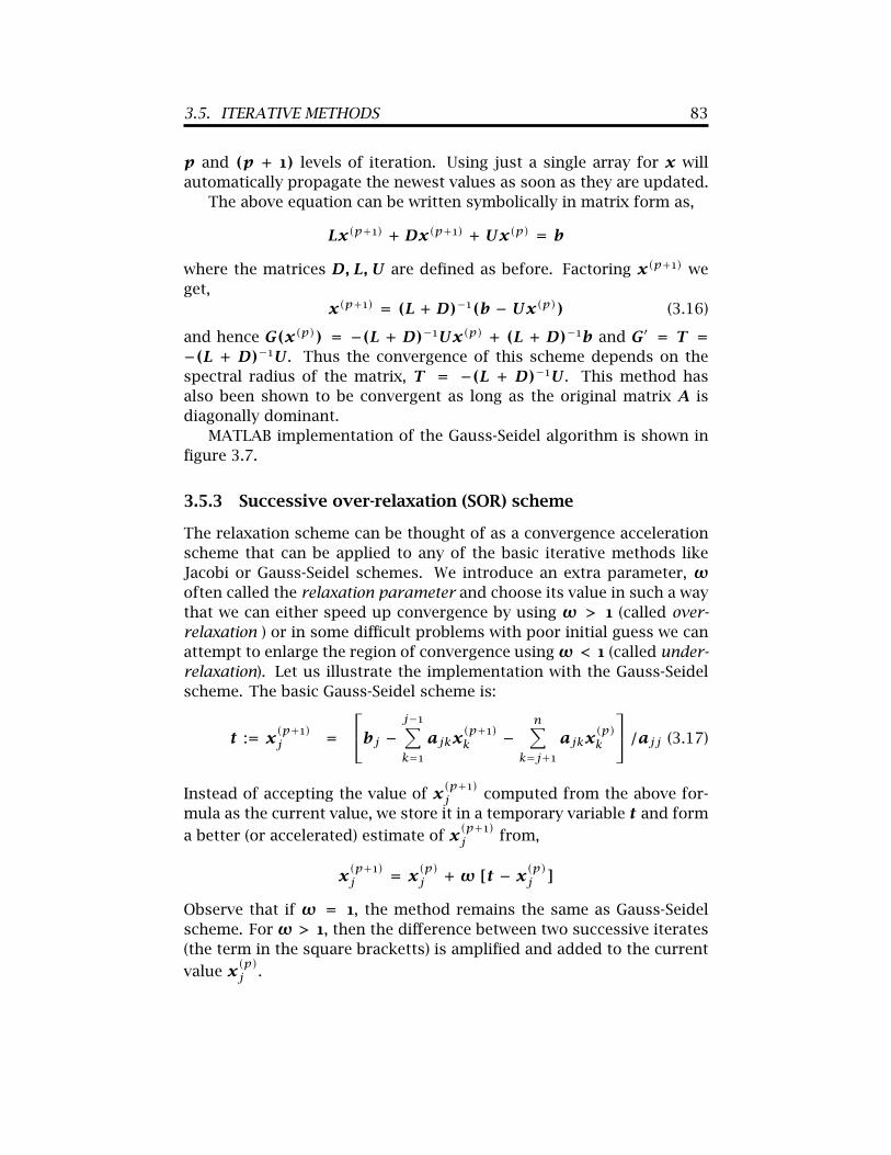
MATLAB implementation of the Gauss-Seidel algorithm is shown infigure 3.7.

3.5.3 Successive over-relaxation (SOR) scheme

The relaxation scheme can be thought of as a convergence accelerationscheme that can be applied to any of the basic iterative methods likeJacobi or Gauss-Seidel schemes. We introduce an extra parameter, ωoften called the relaxation parameter and choose its value in such a waythat we can either speed up convergence by using ω > 1 (called over-relaxation ) or in some difficult problems with poor initial guess we canattempt to enlarge the region of convergence usingω < 1 (called under-relaxation). Let us illustrate the implementation with the Gauss-Seidelscheme. The basic Gauss-Seidel scheme is:

t := x(p+1)j =bj −

j−1∑k=1

ajkx(p+1)k −

n∑k=j+1

ajkx(p)k

/ajj (3.17)

Instead of accepting the value of x(p+1)j computed from the above for-mula as the current value, we store it in a temporary variable t and forma better (or accelerated) estimate of x(p+1)j from,

x(p+1)j = x(p)j + ω [t − x(p)j ]

Observe that if ω = 1, the method remains the same as Gauss-Seidelscheme. For ω > 1, then the difference between two successive iterates(the term in the square bracketts) is amplified and added to the currentvalue x(p)j .


function x=GS(a,b,x,tol,max)% Gauss-Seidel iteration% a - (nxn) matrix% b - column vector of length n% x - initial guess vector x% tol - convergence tolerance% max - maximum number of iterations% Usage x=GS(A,b,x)

m=size(a,1); % get number of rows in matrix an=length(b); % get length of bif (m ˜= n)error(’a and b do not have the same number of rows’)

endif nargin < 5, max=100; endif nargin < 4, max=100; tol=eps; endif nargin == 2error(’Initial guess is required’)

endcount=0;

while (norm(a*x-b) > tol & count < max),x(1) = ( b(1) - a(1,2:n)*x(2:n) )/a(1,1);for i=2:n-1x(i) = (b(i) - a(i,1:i-1)*x(1:i-1) - ...

a(i,i+1:n)*x(i+1:n) )/a(i,i);endx(n) = ( b(n) - a(n,1:n-1)*x(1:n-1) )/a(n,n);count=count+1;

end

if (count >= max)fprintf(1,’Maximum iteration %3i exceeded\n’,count)fprintf(1,’Residual is %12.5e\n ’,norm(a*x-b) )end

Figure 3.7: MATLAB implementation of Gauss-Seidel algorithm


The above opeartions can be written in symbollic matrix form as,

x(p+1) = x(p) + ω[{D−1(b − Lx(p+1) − Ux(p))} − x(p)]

where the term in braces represent the Gauss-Seidel scheme. After ex-tracting x(p+1) from the above equation, it can be cast in the standarditerative from of equation (3.11) as,

x(p+1) = (D + ωL)−1[(1 − ω)D − ωU]x(p) + ω(D + ωL)−1b (3.18)

Thus the convergence of the relaxation method depends on the spectralradius of the matrix T(ω) := (D +ωL)−1[(1 −ω)D −ωU]. Since thismatrix is a function of ω we have gained a measure of control over theconvergence of the iterative scheme. It has been shown (Young, 1971)that the SOR method is convergent for 0 < ω < 2 and that there is anoptimum value ofω which results in the maximum rate of convergence.The optimum value of ω is very problem dependent and often difficultto determine precisely. For linear problems, typical values in the rangeof ω ≈ 1.7 ∼ 1.8 are used.

3.5.4 Iterative refinement of direct solutions

We have seen that solutions obtained with direct methods are proneto accumulation of round-off errors, while iterative methods have thenatural ability to remove such errors. In an attempt to combine the bestof both worlds, one might construct an algorithm that takes the error-prone solution from a direct method as an initial guess to an iterativemethod and thus improve the accuracy of the solution.

Let us illustrate this concept as applied to improving the accuracy ofa matrix inverse. Suppose B is an approximate (error-prone) inverse of agiven matrixA obtained by one of the direct methods outlined in section§3.4. If Bε is the error in B then

A(B + Bε) = I or ABε = (I − AB)

We do not, of course, know Bε and our task is to attempt to estimateit approximately. Premultiplying above equation by B, and recognizingBA ≈ I, we have

Bε = B(I − AB)Observe carefully that we have used the approximation BA ≈ I on theleft hand side where products of order unity are involved and not on theright hand side where difference between numbers of order unity are

3.6. GRAM-SCHMIDT ORTHOGONALIZATION PROCEDURE 86

involved. Now we have an estimate of the error Bε which can be addedto the approximate result B to obtain,

B + Bε = B + B(I − AB) = B(2I − AB)Hence the iterative sequence should be,

B(p+1) = B(p)(2I − AB(p)) p = 0, 1 · · · (3.19)

3.6 Gram-Schmidt orthogonalization procedure

Given a set of n linearly independent vectors, {xi | i = 1, · · · , n} thatare not necessarily orthonormal, it is possible to produce an orthonormalset of vectors {ui | i = 1, · · · , n}.

We begin by normalizing the x1 vector using the norm ||x1|| =√x1 · x1 and call it u1.

u1 = x1||x1||

Subsequently we construct other vectors orthogonal to u1 and normalizeeach one. For example we constructu′2 by subtractingu1 from x2 in sucha way that u′2 contains no components of u1 - i.e.,

u′2 = x2 − c0 u1In the above c0 is to be found in such a way that u′2 is orthogonal to u1.

uT1 · u′2 = 0 = uT1 · x2 − c0 or c0 = uT1 · x2Similarly we have,

u′3 = x3 − c1 u1 − c2 u2Requiring orthogonality with respect to both u1 and u2

uT1 · u′3 = 0 = uT1 · x3 − c1 or c1 = uT1 · x3uT2 · u′3 = 0 = uT2 · x3 − c2 or c2 = uT2 · x3

u′3 = x3 − (uT1 · x3) u1 − (uT2 · x3) u2In general we have,

u′s = xs −s−1∑j=1(uTj · xs) uj us = u′s

||u′s|| s = 2, · · · n; (3.20)

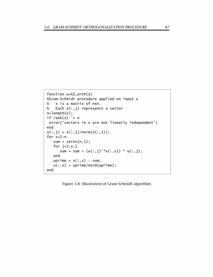
The Gram-Schmidt algorithm is illustrated in figure 3.8. Note thatMATLAB has a built-in functionQ=orth(A)which produces an orthonor-mal set fromA. Q spans the same space asA and the number of columnsin Q is the rank of A.

3.6. GRAM-SCHMIDT ORTHOGONALIZATION PROCEDURE 87

function u=GS_orth(x)%Gram-Schmidt procedure applied on input x% x is a matrix of nxn.% Each x(:,j) represents a vectorn=length(x);if rank(x) ˜= nerror(’vectors in x are not linearly independent’)endu(:,1) = x(:,1)/norm(x(:,1));for s=2:n

sum = zeros(n,1);for j=1:s-1

sum = sum + (u(:,j)’*x(:,s)) * u(:,j);enduprime = x(:,s) - sum;u(:,s) = uprime/norm(uprime);

end

Figure 3.8: Illustration of Gram-Schmidt algorithm

3.7. THE EIGENVALUE PROBLEM 88

3.7 The eigenvalue problem

A square matrix, A, when operated on certain vectors, called eigenvec-tors, x, leaves the vector unchanged excpet for a scaling factor, λ. Thisfact can be represented as,

Ax = λx (3.21)

The problem of finding such eignvectors and eigenvalues is addressedby rewritting equation (3.21) as,

(A − λI) x = 0

which represents a set of homogeneous equations that admit non-trivialsolutions only if

det(A − λI) = 0.i.e., only certain values of λ will make the above determinant zero. Thisrequirement produces an n-th degree polynomial in λ, called the char-acteristic polynomial. Fundamental results from algebra tell us that thispolynomial will have exactly n roots, {λj|j = 1 · · · n} and correspond-ing to each root, λj we can determine an eigenvector, xj from

(A − λjI) xj = 0.

Note that if, xj satisfies the above equation, then axj will also satsify thesame equation. Viewed alternately, since the det(A−λjI) is zero, xj canbe determined only up to an unknown constant - i.e., only the directionof the eignvector can be determined, its magnitude being arbitrary.

The MATLAB built-in function [V,D]=eig(A) computes all of theeigenvalues and the associated eigenvectors.

Example

Determine the eigenvalues and eigenvectors of the matrix A defined be-low.

A = 2 4 34 4 33 3 5

A typical MATLAB session follows.


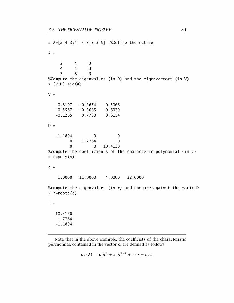
» A=[2 4 3;4 4 3;3 3 5] %Define the matrix

A =

2 4 34 4 33 3 5

%Compute the eigenvalues (in D) and the eigenvectors (in V)» [V,D]=eig(A)

V =

0.8197 -0.2674 0.5066-0.5587 -0.5685 0.6039-0.1265 0.7780 0.6154

D =

-1.1894 0 00 1.7764 00 0 10.4130

%compute the coefficients of the characteric polynomial (in c)» c=poly(A)

c =

1.0000 -11.0000 4.0000 22.0000

%compute the eigenvalues (in r) and compare against the marix D» r=roots(c)

r =

10.41301.7764-1.1894

Note that in the above example, the coefficiets of the characteristicpolynomial, contained in the vector c, are defined as follows.

pn(λ) = c1λn + c2λn−1 + · · · + cn+1


3.7.1 Left and right eigenvectors

The eigenvector x, defined in equation (3.21), is called the right eigen-vector, since the matrix product operation is performed from the right.Consider the operation with a vector y

y′A = y′λ (3.22)

Since equation (3.22) can be written as

y′(A − λI) = 0

the criterion for admitting nontrivial solutions is still the same, viz.

det(A − λI) = 0.

Thus the eigenvalues are the same as those defined for the right eigen-vector. If A is symmetric, then taking the transpose of equation (3.22)leads to equation (3.21) pointing out that the distinction between the leftand right eigenvectors disappear. However for a nonsymmetric matrix,A there is a set of left {xi|i = 1 · · · n} and right {yj|j = 1 · · · n}eigenvectors that are distinct and form a bi-orthogonal set as shown be-low.

3.7.2 Bi-orthogonality

As long as the eigenvalues are distinct, the left and right eigenvectorsform a bi-orthogonal set. To demonstrate this, take the left product ofequation (3.21) with y′j and the right product of equation (3.22) with xi.These lead respectively to

y′jAxi = λiy′jxiy′jAxi = λjy′jxi

Subtracting one from the other, we get,

0 = (λi − λj)y′jxi.

Since λi and λj are distinct, we get

y′jxi = 0 ∀i 6= j

which is the condition for bi-orthogonality.


3.7.3 Power iteration

A simple algorithm to find the largest eigenvalue and its associatedeigenvector of a matrix A is the power iteration scheme. Conceptuallythe algorithm works as follows. Starting with any arbitrary vector, z(0),produce a sequence of vectors from

y(p+1) = Az(p)

y(p+1) = k(p+1)z(p+1) p = 0, 1, · · ·The second step above is merely a scaling operation to keep the vectorlength z(p) bounded. The vector z(p) converges to the eigenvector x1corresponding to the largest eigenvalue as p → ∞.

The reason why it works can be understood, by begining with a spec-tral representation of the arbitrary vector, z(0) and tracing the effect ofeach operation, i.e.,

z(0) =∑iαixi

y(1) = Az(0) =∑iαiAxi =

∑iαiλixi

y(2) = Az(1) = Ay(1)

k(1)= 1k(1)

∑iαiλiAxi = 1

k(1)∑iαiλ2ixi

Repeating this process we get,

y(p+1) = Az(p) = 1∏pj k(j)

∑iαiλ

p+1i xi

Factoring the largest eigenvalue, λ1,

y(p+1) = Az(p) = λp+11∏pj k(j)

∑iαi(λiλ1

)p+1xi

Since (λi/λ1) < 1 for i > 1 only the first term in the summationsurvives as p → ∞. Thus y(p) → x1, the eigenvector corresponding tothe largest eigenvalue.

Several other features also become evident from the above analysis.

• The convergence rate will be faster, if the largest eigenvalue is wellseparated from the remaining eigenvalues.

• If the largest eigenvalue occurs with a multiplicity of two, then theabove sequence will not converge, or rather converge to a subspacespaned by the eigenvectors corresponding to the eigenvalues thatoccur with multiplicity.


function [Rayleigh_Q,V] = Power(T,MaxIt)%Power iteration to find the largest e.value of T

if nargin < 2,MaxIt = 100;

end

n=length(T); %Find the size of Tz_old=rand(n,1); %Generate random vector, zz_new=z_old/norm(z_old); %Scale itCheck_sign=1; count = 0; %Initializewhile (norm(z_old-z_new) > 1.e-10 & count < MaxIt),

count = count + 1;z_old=z_new*Check_sign;z_new=T*z_new;z_new=z_new/norm(z_new);Check_sign=sign((z_new’*(T*z_new))/(z_new’*z_new));

endif (count >= MaxIt)

error(’Power iteration failed to converge’)end%Compute the Rayliegh quotientV=z_new;Rayleigh_Q=(z_new’*(T*z_new))/(z_new’*z_new);

Figure 3.9: MATLAB implementation of power iteration

• If the initial guess vector does not contain any component in thedirection of x1, then the sequence will converge to the next largesteigenvalue. This can be acheived by making the guess vector, z(0),orthogonal to the known eigenvector, x1.

3.7.4 Inverse iteration

To find the smallest eigenvalue of a given a matrix A, the power itera-tion could still be applied, but on the inverse of matrix A. Consider theoriginal eigenvalue problem

Axi = λixi.


Premultiply by A−1 to get,

A−1Axi = λiA−1xiwhich can be rewritten as,

1λixi = A−1xi.

Hence it is clear that the eigenvalues, µi of A−1 viz.

µixi = A−1xiare related to eigenvalues, λi of A through,

λi = 1µi.

Although the illustration below uses the inverse of the matrix, inreality there is no need to find A−1 since power iteration only requirescomputation of a new vector y from a given vector z using,

y(p+1) = A−1z(p).This can be done most effectively by solving the linear system

Ay(p+1) = z(p)

using LU factorization, which needs to be done only once.

3.7.5 Shift-Inverse iteration

To find the eigenvalue closest to a selected point, σ, the power iterationcould be applied to the matrix (A−σI)−1, which is equivalent to solvingthe eigenvalue problem

(A − σI)−1xi = µixi.This can be rewritten as,

1µixi = (A − σI)xi = Axi − σxi = (λi − σ)xi.

Hence it is clear that the eigenvalues, µi of (A − σI)−1 are related toeigenvalues, λi of A through,

λi = 1µi+ σ.


As in the previous section, there is no need to find the inverse sincepower iteration only requires computation of a new vectory from a givenvector z using,

y(p+1) = (A − σI)−1z(p).This can be done most effectively by solving the linear system

(A − σI)y(p+1) = z(p)

using LU factorization of (A − σI), which needs to be done only once.

Example

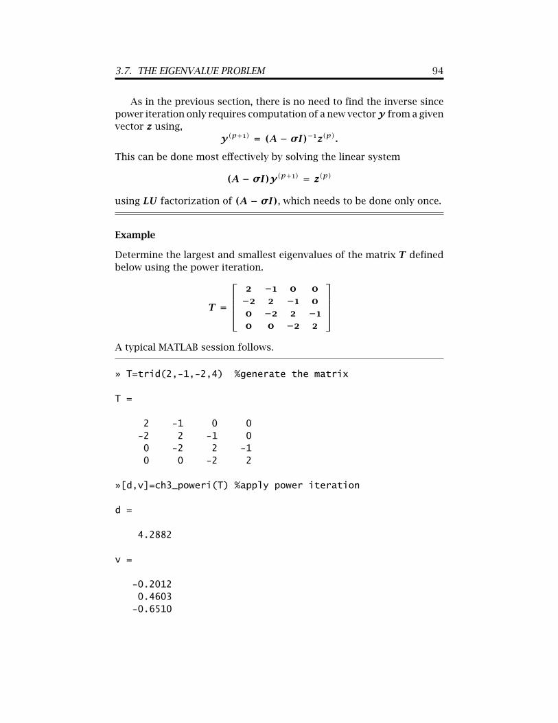
Determine the largest and smallest eigenvalues of the matrix T definedbelow using the power iteration.

T =

2 −1 0 0−2 2 −1 00 −2 2 −10 0 −2 2

A typical MATLAB session follows.

» T=trid(2,-1,-2,4) %generate the matrix

T =

2 -1 0 0-2 2 -1 00 -2 2 -10 0 -2 2

»[d,v]=ch3_poweri(T) %apply power iteration

d =

4.2882

v =

-0.20120.4603-0.6510


0.5690

»max(eig(T)) %Find the largest e-value from ‘‘eig’’ function

ans =

4.2882

%Find the smallest e. value»mu=ch3_poweri(inv(T));»lambda=1/mu

lambda =

-0.2882»min(eig(T))

ans =

-0.2882

»%Find the e.value closest to 2.5»sigma=2.5;»mu=ch3_poweri(inv(T-sigma*eye(4)))

mu =

2.6736

»lambda=sigma+1/mu

lambda =

2.8740%verfiy using ‘‘eig’’»eig(T)

ans =

-0.28824.28822.8740

3.8. SINGULAR VALUE DECOMPOSITION 96

1

3

4

5

6

2v12

v35

v46

v34p1

p5

p6

p2

Figure 3.10: Laminar flow in a pipe network

1.1260

3.7.6 Wei-Prater analysis of a reaction system

3.8 Singular value decomposition

3.9 Genaralized inverse

3.10 Software tools

3.10.1 Lapack, Eispack library

3.10.2 MATLAB

3.10.3 Mathematica

3.11 Exercise problems

3.11.1 Laminar flow through a pipeline network

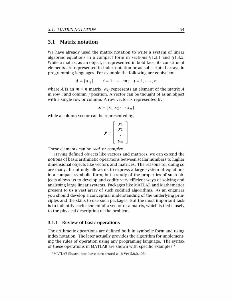
Consider laminar flow through the network shown in figure 3.10. Thegoverning equations are the pressure drop equations for each pipe ele-ment i − j and the mass balance equation at each node.The pressure drop between nodes i and j is given by,

pi − pj = αijvij where αij =32µlijd2ij

(3.23)

3.11. EXERCISE PROBLEMS 97

The mass balance at node 2 is given, for example by,

d212v12 = d223v23 + d224v24 (3.24)

Similar equations apply at nodes 3 and 4. Let the unknown vector be

x = [p2 p3 p4 v12 v23 v24 v34 v35 v46]There will be six momentum balance equations, one for each pipe ele-ment, and three mass balance (for incompressible fluids volume balance)equations, one at each node. Arrange them as a system of nine equationsin nine unknowns and solve the resulting set of equations. Take the vis-cosity of the fluid, µ = 0.1Pa · s. The dimensions of the pipes are givenbelow.

Table 1

Element no 12 23 24 34 35 46

dij (m) 0.1 0.08 0.08 0.10 0.09 0.09lij (m) 1000 800 800 900 1000 1000

a) Use MATLAB to solve this problem for the specified pressures ofp1 = 300kPa and p5 = p6 = 100kPa. You need to assemblethe system of equations in the form A x = b. Report flops. Whenreporting flops, report only for that particular operation - i.e., ini-tialize the counter using flops(0) before every operation.

• Compute the determinant of A. Report Flops.

• Compute the LU factor ofA using built-in function lu. Reportflops. What is the structure of L? Explain. The function LUprovided in the lecture notes will fail on this matrix. Why?

• Compute the solution using inv(A)*b. Report flops.

• Compute the rank of A. Report Flops.

• Since A is sparse ( i.e., mostly zeros) we can avoid unnecessaryoperations, by using sparse matrix solvers. MATLAB Ver4.0(not 3.5) provides such a facility. Sparse matrices are storedusing triplets (i, j, s) where (i, j) identifies the non-zero en-try in the matrix and s its corresponding value. The MATLABfunction find(A) examines A and returns the triplets. Use,


» [ii,jj,s]=find(A)

Then construct the sparse matrix and store it in S using

» S=sparse(ii,jj,s)

Then to solve using the sparse solver and keep flops count,use

» flops(0); x = S\b; flops

Compare flops for solution by full and sparse matrix solution.To graphically view the structure of the sparse matrix, use

» spy(S)

Remember that you should have started MATLAB under X-windows for any graphics display of results!

• Compute the determinant of the sparse matrix, S (should bethe same as the full matrix!). Report and compare flops.

b) Find out the new velocity and pressure distributions when p6 ischanged to 150kPa.

c) Suppose the forcing (column) vector in part (a) is b1 and that inpart (b) is b2, report and explain the difference in flops for the fol-lowing two ways of obtaining the two solutions using the sparsematrix. Note that in the first case both solutions are obtained si-multaneously.

» b = [b1, b2];flops(0);x = S\b,flops» flops(0);x1 = S\b1, x2 = S\b2,flops

Repeat the above experiment with the full matrix, A and reportflops.

d) Comment on how you would adopt the above problem formulationif a valve on line 34 is shut so that there is no flow in that line 34.

3.11.2 Grahm-Schmidt procedure

Consider the vectors

x1 = [1234] (3.25)

x2 = [1212] (3.26)


x3 = [2131] (3.27)

x4 = [2154] (3.28)

• Check if they form a linearly independent set.

• Construct an orthonormal set using the Grahm-Schmidt procedure

3.11.3 Power iteration

Consider the matrix, A given below.

A =

2.0 + 4.0i -1.0 - 2.0i 0 0-2.0 - 4.0i 2.0 + 4.0i -1.0 - 2.0i 0

0 -2.0 - 4.0i 2.0 + 4.0i -1.0 - 2.0i0 0 -2.0 - 4.0i 2.0 + 4.0i

Use the power iteration algorithmn given in Fig. 3.9 to solve thefollowing problems.

• Find the largest eigenvalue. [Ans: 4.2882 + 8.5765i]

• Find the smallest eigenvalue. [Ans: -0.2882 - 0.5765i]

• Find the eigenvalue closest toσ = (1+2i). [Ans: 1.1260 + 2.2519i]

System of linear algebraic equation - sites.ualberta.cakumar/handouts/chap3.pdf · 3.1. MATRIX...

Documents

Transcript of System of linear algebraic equation - sites.ualberta.cakumar/handouts/chap3.pdf · 3.1. MATRIX...